Vertical distribution of pollution trapped by wintertime surface inversions in Fairbanks, Alaska, during the ALPACA experiment

Air pollution in cold wintertime urban areas is a ubiquitous problem. Surface temperature inversions under low wind conditions and surface emissions lead to the formation of a shallow polluted surface layer (PSL). The presence of this PSL is well documented, but its height, the rates of exchange with the background atmosphere, and the interplay between vertical mixing and chemistry remain poorly quantified. Here we provide quantitative insights into this coupled chemistry-transport system using observations and modeling of vertical pollutant profiles.

Long-path Differential Optical Absorption Spectroscopy of vertical trace gas profiles during the 2022 Alaskan Layered Pollution and Chemical Analysis (ALPACA) experiment in Fairbanks, Alaska, quantitatively track the frequent establishment of PSLs with heights of 20–40 m, which sometimes persist for several days. PSL trace gas mixing ratios often plateau at levels of up to 35 ppb SO₂, 60 ppb NO₂, 2.5 ppb HONO, 7 ppb HCHO, and low ozone as a result of surface emissions, gas-phase chemistry, and ineffective mixing with the background atmosphere. Parameterizing vertical mixing with observed surface temperature gradients and wind speed in the PACT-1D chemistry and transport model leads to excellent agreement of modeled and measured trace gas profiles. The PACT-1D transport scheme determines the residence time of pollutants within the PSL to be 1–4 h, confirming the strong influence of atmospheric mixing on the composition of sustained PSL events. Altitude-dependent ozone and NO_x chemistry highlight the strong coupling between mixing and chemistry, which must be considered to quantify pollutant concentrations accurately in shallow PSLs.

1 Introduction

Wintertime air pollution is a ubiquitous problem in northern and many mid-latitude cities. Urban areas, such as the Salt Lake Valley, Utah (Lareau et al., 2013), Fairbanks, Alaska, (Tran and Mölders, 2011; Mölders et al., 2012; Ward et al., 2012; Cesler-Maloney et al., 2022; Simpson et al., 2024), and megacities in China (e.g. Wang et al., 2016, 2014; Li et al., 2005) frequently experience high levels of SO₂, NO_x, particulate matter, and other pollutants. These increased pollutant concentrations have been associated with negative health effects (e.g. Laskin, 2006; Bell and Davis, 2001; Beard et al., 2012; Pope III et al., 1999; Pope, 1991) and there is thus an urgent need to study meteorological, physical, and chemical mechanisms underlying the formation of wintertime air pollution in order to support the development of successful mitigation strategies.

Urban pollution in winter is often linked to stable surface temperature inversions (SSI) that trap anthropogenic emissions in a shallow polluted surface layer (PSL), as well as low wind speeds that prevent the horizontal dispersion of pollutants. SSIs form when shortwave radiative heating is small compared to larger longwave surface heat loss, and low wind speeds reduce shear-induced turbulence (Bowling et al., 1968; Mahrt, 2014, 1999; Garratt, 1994; Stull, 1988). Conditions for the formation of radiative SSIs are most commonly met at night, leading to the stable nocturnal boundary layer, and in winter, when they can persist for several days. Advection of warm air over a cold surface can also lead to the formation of temperature inversions and thus stable surface layers (Anderson and Neff, 2008; Whiteman et al., 2001; Lu and Zhong, 2014; Largeron and Staquet, 2016). Both mechanisms can occur simultaneously to form a SSI. Low wind speeds affect surface pollution also by making horizontal dispersion of pollutants and advection of clean air from surrounding areas less efficient. It is often challenging to separate the effect of low wind speeds on SSI formation and advection when studying wintertime PSL formation. When specific topographic features, such as valleys or bowls, contribute to these factors, and the SSI persists for more than a day, it is often classified as a persistent cold air pool (Lareau et al., 2013; Hallar et al., 2021; Simpson et al., 2024). The formation of high latitude SSI layers has been studied extensively over sea ice and ice cap areas, as summarized by Anderson and Neff (2008). However, despite the presence of this surface inversion during wintertime pollution events, many aspects of its formation and its height are not well constrained by observations. In addition, quantitative modeling of surface vertical mixing in and out of the PSL, and the influence of associated temperature gradients, remain an unresolved challenge (Beare et al., 2006; Hallar et al., 2021; Simpson et al., 2024).

Wintertime urban air chemistry has received increased attention in recent years, in part motivated by unusually high particulate sulfate concentrations in Chinese cities (Wang et al., 2014, 2016; Cheng et al., 2016), as well as recent results from the 2022 Alaskan Layered Pollution and Chemical Analysis (ALPACA) experiment in Fairbanks, AK, (e.g. Moon et al., 2024; Campbell et al., 2024; Dingilian et al., 2024; Simpson et al., 2024). Cold temperatures, small actinic fluxes, high concentrations of primary pollutants, and the presence of snow impact the chemical processing of trace gases in the winter PSL. The PSL is typically depleted in ozone and has very high levels of NO_x and PM. This behavior is similar to that previously seen in the urban nocturnal boundary layer (NBL), where nocturnal emissions of NO deplete ozone concentrations while forming NO₂ (Stutz et al., 2004; Geyer and Stutz, 2004; Wong et al., 2011; Tuite et al., 2021; Brown et al., 2007a, b; Brown and Stutz, 2012). However, in contrast to summertime polluted NBLs, which break up at sunrise and re-form again after sunset, wintertime PSLs often persist for days leading to extended periods of low ozone. Low ozone concentrations in the PSL change the radical chemistry in the PSL, as ozone is a precursor to reactive radicals such as OH and itself oxidizes certain hydrocarbons. Lack of ozone, together with small actinic fluxes, raises the question of the role of gas-phase radical chemistry in the PSL and whether aerosol multiphase chemistry plays the dominant role in transforming pollutants. For example, gas-phase oxidation of SO₂ has been found to be slow and the formation of sulfate and hydromethanesulfonate (HMS) has been explained by aerosol chemistry, including new aqueous phase sulfite reactions with NO₂ and HCHO (Cheng et al., 2016; Gao et al., 2016; Moch et al., 2018; Wang et al., 2016; Zhang et al., 2023; Dingilian et al., 2024; Campbell et al., 2024). These results show that further studies are needed to improve our knowledge of wintertime air pollution chemistry.

Surface temperature inversions are a crucial aspect of the formation of the winter PSL and consequently of air pollution chemistry. However, little quantitative information is available on the interplay between vertical mixing within the PSL and with the background atmosphere and how this impacts chemical processes. Our understanding of the coupling of vertical mixing and chemistry is incomplete largely because there are very few observations of the vertical distribution of trace gases and PM in affected urban areas. Many studies only provide temporal snapshots through balloon soundings or aircraft profiling, rather than continuous data on the vertical pollutant distribution (Chen et al., 2002; Baasandorj et al., 2017; Wang et al., 2018; Franchin et al., 2018; Hallar et al., 2021; Cesler-Maloney et al., 2022; Pohorsky et al., 2025). Others provide continuous data at two altitudes and do not allow the determination of the PSL height (Cesler-Maloney et al., 2022). In addition, only a limited number of pollutants and PM are observed. Thus, there is a clear need to provide better data on the vertical distribution of pollution gases in the wintertime urban boundary layer to characterize the coupling of mixing and chemistry in the PSL.

The study of wintertime air pollution also requires high-resolution models to resolve the vertical scale of the PSL, which is typically on the order of 10–100 m. Typical air quality models have difficulties resolving the vertical extent of the PSL and often do not adequately capture the weak vertical mixing in the PSL due to a lack of accurate parameterization for mixing in stable boundary layers (Simpson et al., 2024; Baker et al., 2011; Sun et al., 2021; Adler et al., 2023). One-dimensional chemistry and transport models have been successfully used to study other chemical environments under similar meteorological conditions, constraining mixing by observations or meteorological models (Thomas et al., 2011; Geyer and Stutz, 2004; Tuite et al., 2021) or using simplified parameterizations of eddy diffusivities (Wong et al., 2011; Cao et al., 2016; Ahmed et al., 2022; Herrmann et al., 2019). A similar approach has not yet been used for wintertime urban air pollution, and could provide important insights into the various coupled transport-chemistry mechanisms.

To advance our understanding of the chemistry-transport environment of the PSL continuous measurements of the vertical distribution of reactive gases, such as SO₂, O₃, and NO_x, are needed. Interpretation of these profiles is challenging, and we propose that it is best achieved with a high-resolution, observation driven model that can capture transport and chemistry at the spatial scale of the PSL. Here, we present such observations and model calculations for the example of Fairbanks, AK, which is known to experience persistent PSL conditions in winter, and is also one of the most polluted cities in the USA in winter (Simpson et al., 2024; Cesler-Maloney et al., 2022; Ye and Wang, 2020). Our study aims to better understand the complex interaction between emissions, chemistry, and transport that ultimately determines the fate of anthropogenic pollutants in the PSL. Specifically, we will answer the following scientific questions:

• What are the properties of the PSL, including height, pollutant concentrations, vertical mixing, and how can these be monitored on a continuous basis?

• How is PSL formation and persistence related to surface temperature inversions and wind speed in Fairbanks?

• What role does the PSL play for surface pollutant concentrations and how is atmospheric chemistry coupled to mixing?

• What is the residence time of trace gases in the PSL?

To answer these questions, we performed observations with UCLA's Long-Path Differential Optical Absorption Spectroscopy (LP-DOAS) instrument and developed a new approach to retrieve mixing ratio profiles from path averaged data (Sect. 2). We set up UCLA's Platform for Atmospheric Chemistry and Transport in one dimension (PACT-1D) model to simulate Fairbanks atmospheric chemistry (Sect. 4), using a new parameterization of vertical eddy diffusivity that is based on a statistical analysis of the PSL heights measured with the LP-DOAS and vertical temperature gradients (Sect. 4.2). This new parameterization yields excellent agreement with vertical profile observations (Sect. 4.4), giving us insight into the timescale of the evolution of PSL, the link between chemistry and transport, and the residence time of pollutants in the PSL (Sect. 5).

2 Observations of Vertical Profiles of Trace Gases and Temperature

The data presented here was measured by UCLA’s LP-DOAS instrument (Stutz and Platt, 1997; Tsai et al., 2014; Platt and Stutz, 2008) and in-situ sensors during the 2022 ALPACA field experiment (Simpson et al., 2024). The observational period of the LP-DOAS extended from 22 January to 23 February 2022. Environmental conditions during ALPACA included cold periods with high pollution levels interspersed with periods of enhanced pollutant export and consequently low pollution levels (Simpson et al., 2024). The details of these conditions will be discussed in Sect. 3. In the following sections, we present the instrumental setup as well as the data analysis of the various instruments.

2.1 LP-DOAS observations

LP-DOAS measurements are based on the identification and quantification of narrow-band trace gas absorption features in the open atmosphere (Platt and Stutz, 2008). During ALPACA a 120 cm focal length, 30 cm diameter fiber telescope was used to send a collimated beam of light from a laser-driven Xe light source (Energetiq LDLS 99X) onto arrays of quartz corner-cube retro-reflectors. The reflected light was captured by the telescope and transferred through a mode mixer (Stutz and Platt, 1997) to a thermally stabilized 300 mm focal length Czerny-Turner spectrometer (ACTON Pro 300 at 20 °C) and a CCD detector array cooled to −70 °C (Teledyne PIXIS). The LP-DOAS telescope was located on the top floor of the Lacey-Street Parking Garage (64.844° N, −147.716° E) in downtown Fairbanks at an altitude of 17 m above ground level (m a.g.l.). To measure the vertical trace gas profile, four reflector arrays were mounted at different altitudes northeast of the telescope (Fig. 1). The lowest path averaged trace gas concentrations along an 1154 m long path over an height interval of 12–17 m a.g.l. Three other reflectors were mounted along Birch Hill at 73, 115, and 191 m altitude at a distance of 3.6 to 4 km (Fig. 1). The telescope was aimed sequentially at each reflector array using automated stepper motors for rotation in azimuth and elevation, providing a complete vertical scan every 30–60 min.

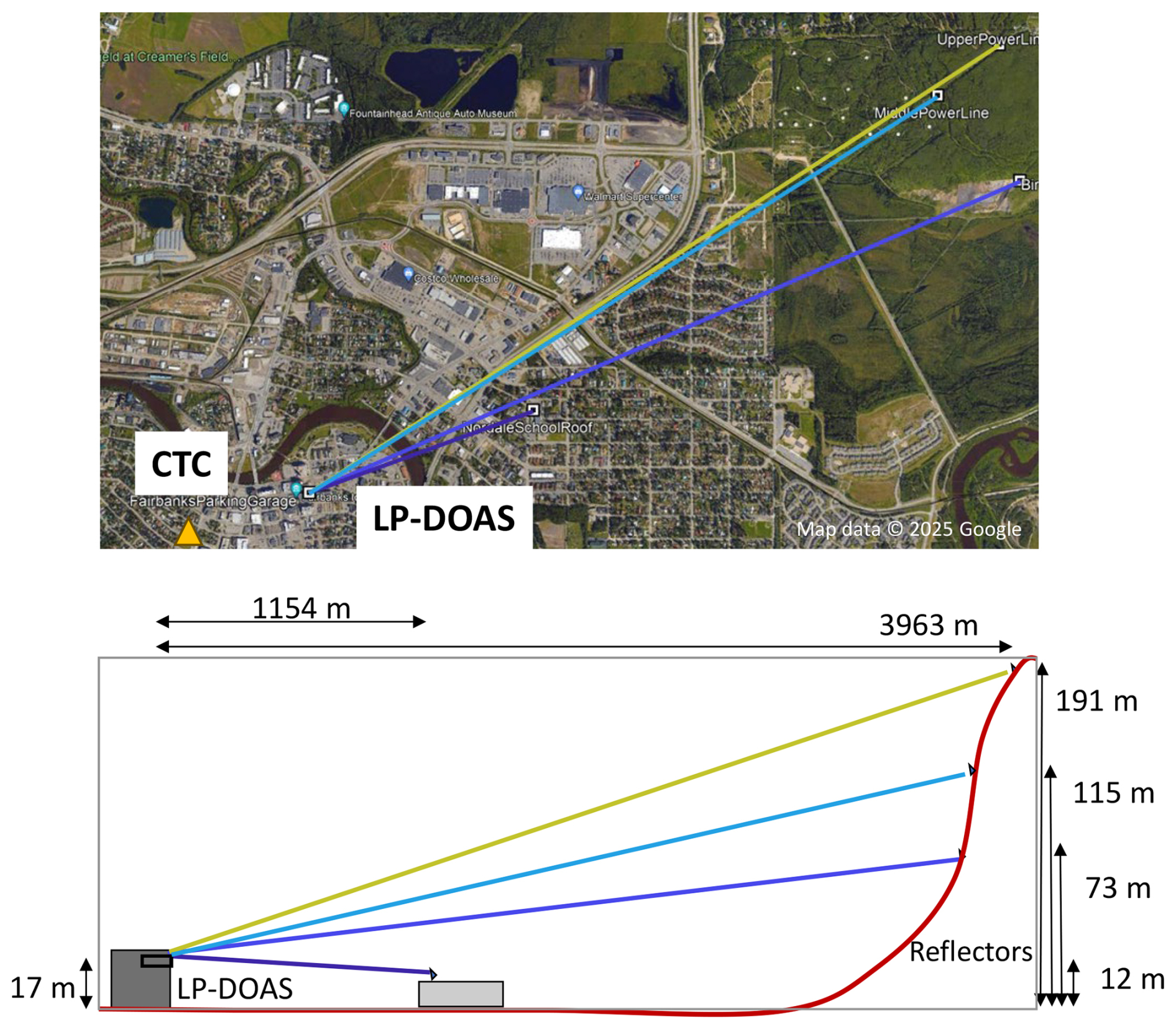
Figure 1 Sketch of the LP-DOAS instrument and location of absorption paths and in-situ observations. In-situ measurements were located at the CTC building marked by the yellow triangle. The distance between the LP-DOAS and the CTC building is approximately 500 m.

Trace gas mixing ratios were retrieved from LP-DOAS absorption spectra using established DOAS retrievals (Stutz and Platt, 1996; Platt and Stutz, 2008) in various wavelength windows between 280–380 nm. This procedure also calculates the error of the measurements. Accuracy of the LP-DOAS path averaged trace gas concentrations are determined by the uncertainty in the absorption cross section and are in the range of 3 %–8 %. Details on the retrieval procedure and detection limits are given in Sect. S1 in the Supplement.

2.2 In-situ observations

In-situ instruments were located near the University of Alaska Fairbanks Community and Technical College field site (CTC, 64.841° N, −147.727° E) (Fig. 1). SO₂ was measured in-situ at 3 m a.g.l. with a Thermo Scientific 43C instrument located in a stationary trailer parked next to the CTC building. Ozone and NO_x were measured at the same location and height using a Thermo Scientific 49C and 42C instruments, respectively. A second ozone monitor (Teledyne 400E) was deployed at Birch Hill at an altitude of 158 m above the valley floor. Details on these observations can be found in the Supplement.

Temperatures were measured with aspirated thermometers at 3, 6, and 11 m on a small tower in an parking lot adjacent to the CTC building, and at 23 m a.g.l. above the roof of the buildings elevator shaft house (Cesler-Maloney et al., 2022). The temperature measurement had a precision better than 0.15 °C, allowing the derivation of vertical temperature gradients. Wind speed and direction were also measured at 23 m a.g.l. on the CTC roof using an RM Young 1005 monitor. A comparison of the 11 m and 10 m to 3 m temperature gradients show that the CTC gradients are ∼14 % lower than those at the the Alaska National Core Multi-Pollutant Monitoring Station site (NCORE), which is about 500 m north of the CTC building (Simpson et al., 2024). Comparison of 23 m wind speeds on the CTC roof with 10 m wind speeds at the nearby NCORE site yields good agreement (Fig. S8 in the Supplement).

2.3 Profile and PSL height retrievals

Interpretation of vertical profiles of LP-DOAS path-averaged concentrations is challenging due to overlapping altitude intervals. While a sequential difference approach has been used (Wang et al., 2006; Stutz et al., 2004; Tsai et al., 2014), we developed a different approach here that is better suited to study the polluted surface layer. Our approach is also able to incorporate in-situ observations, when available. The basic idea of our retrieval is the assumption that the shape of the trace gas concentration profile, C(z), can be described by a sigmoid function:

$$\begin{array}{}\text{(1)}& C\left(z\right)=C_a+C_b\times \left(\mathrm{1}-{\displaystyle \frac{\mathrm{1}}{\mathrm{1}+\exp (-(z-H)/M)}}\right)\end{array}$$

Here, z is altitude, and C_a and C_b are two parameters that control the concentrations at the low and high end of the profiles. M is a parameter that broadly describes the slope of the transition. H is an altitude offset, which, for box-shaped profiles (M<1) can be interpreted as the half-point between C_a and C_b. It should be noted that C_a and C_b are only equivalent to surface and z=200 m concentrations when M is very small and $H<\sim \mathrm{200}$ m. Equation (1), with its four free parameters, allows for the description of a broad set of profiles as illustrated in Fig. S3. Combination of the four parameters can describe many shapes from box-like, linear and curved decreasing, and constant profiles (Fig. S3). Most parameter combinations in Eq. (1) yield profiles that decrease with altitude, which matches the behavior of SO₂, NO₂, HONO, and HCHO, which typically have higher concentration at the ground. In contrast, ozone often has lower concentrations at the surface. Therefore, Eq. (1) has to be slightly modified to allow for the inverted ozone altitude profile: $C\left(z\right)=C_a+C_b\times \mathrm{1}/(\mathrm{1}+\exp (-(z-H)/M\left)\right)$. Because the four parameters in Eq. (1) do not represent direct physical measures we will not use them in our analysis, but rather interpret the resulting profiles C(z). We will justify the choice of a sigmoid function in Sect. 4.4 when we compare the retrieval results and with profiles from a 1D chemistry and transport model.

To derive the four parameters in Eq. (1), we first interpolated the path-averaged LP-DOAS data from the upper three light paths onto the measurement time of the lowest light path, while propagating the measurement error to the interpolated data. Because path-averaged data varies slowly, a linear interpolation was chosen. Similarly, we averaged the in-situ data over the time interval of the lowest light path measurements. A non-linear Levenberg–Marquardt fit then optimized the model function describing the altitude averaged, time interpolated, LP-DOAS data and the concentration of in-situ observations. The function calculates Eq. (1) on a regular 1 m grid from the surface to 200 m altitude and then numerically integrates the concentration vector in the altitude intervals of the respective LP-DOAS light paths. In-situ data are taken from the grid cell closest to the exact measurement altitude. The non-linear fit then optimizes C_a, C_b, M and H to find the best agreement of the function output to the observations.

To quantify the impact of measurement errors on the retrieval results, we chose a Monte-Carlo approach. We performed the retrieval 250 times while randomly varying the input data to the retrieval using a Gaussian probability density function with the observation as the mean and the measurement error as the standard deviation. We then averaged the 250 retrieved profiles and used the standard deviation as our profile mixing ratio error. From these profiles, we determine the surface layer height (SLH) as the altitude in which the mixing ratio is the midpoint between C(0 m) and C(200 m), and the uncertainty of this value. Our retrieval assumes horizontal homogeneity within the extent of our light paths. The very good agreement of NO₂ and SO₂ on the lowest light path with the in-situ observations (Fig. 2) confirms that this path is representative of surface mixing ratios in downtown Fairbanks. In the presence of a PSL, the volume probed by the upper three light paths is dominated by background air, which is typically well mixed vertically and horizontally. Our retrievals confirm that in most cases air above a well-developed PSL does not show a vertical profile within the uncertainties (see below). In the case of a well-mixed atmosphere, horizontal inhomogeneities are also reduced. In cases of intermediate mixing this assumption may, however, not strictly hold. Because horizontal inhomogeneities would distort vertical trace gas profiles, we can use the agreement of the retrieved point and altitude-averaged mixing ratios with the observations to assess whether horizontal inhomogeneities would prevent interpretation of our vertical profiles. Figures S4 and S5 show that the agreement of the retrieved and observed mixing ratios for O₃ and NO₂ is excellent. In particular, the agreement between the 3 m surface mixing ratios and the 158 m Birch Hill ozone in situ measurements with the retrieval results show that our retrievals are not noticeably impacted by horizontal inhomogeneities and that we can use the retrieved profiles to analyze the vertical structure of the Fairbanks atmosphere.

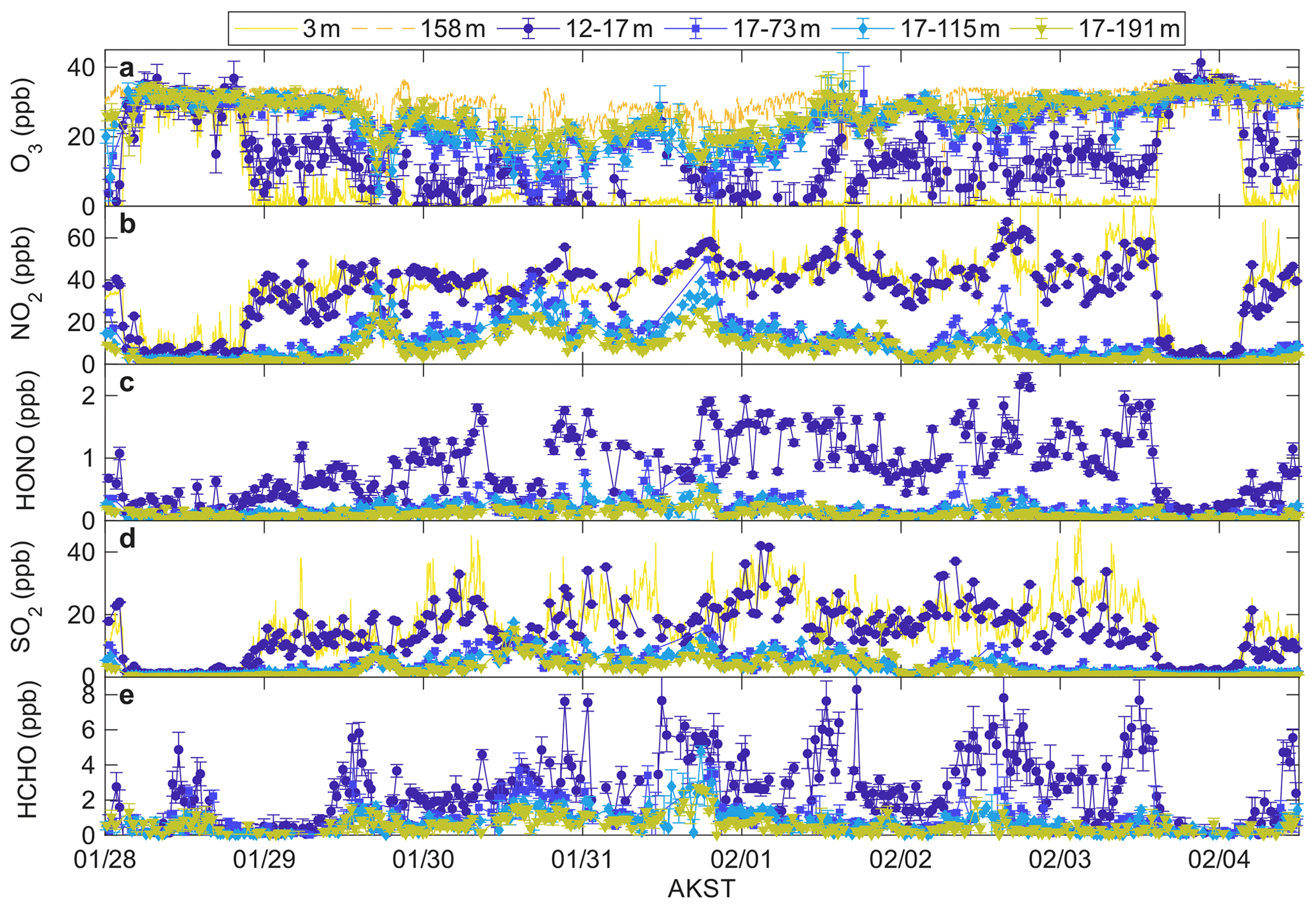
Figure 2 Overview of one week of path-averaged LP-DOAS data along the four different lightpaths using the same color coding as in Fig. 1. Surface (3 m) in-situ data is shown as a yellow line, while the Birch Hill data (158 m) is shown as a dashed dark yellow line. The full dataset is shown in Fig. S1.

3 Observational Results

3.1 Path-averaged concentrations

Path-averaged mixing ratios from the LP-DOAS instrument show large variability in time and altitude throughout the ALPACA experiments (Fig. 2). Ozone mixing ratios were consistently highest on the upper light path (dark yellow in Fig. 2) and lowest in the 12–17 m path (dark blue markers in Fig. 2). The other paths were typically in between these two extremes. The smallest mixing ratio of ozone was observed by the in-situ instrument at 3 m a.g.l. (yellow line in Fig. 2), where ozone often dropped to within measurement error of zero. For much of the experiment, the upper path reflected background levels of O₃ of 30 to 35 ppb, which is also reflected in the in-situ ozone observations on Birch Hill (158 m altitude in Fig. 2). Occasionally, ozone mixing ratios aloft dropped below 20 ppb.

Overall, NO₂ exhibits the opposite behavior from ozone, with highest mixing ratios close to the surface and lowest mixing ratio aloft. The lower path NO₂ agrees well with the in-situ observations at nearby CTC. The rapid NO+O₃ reaction in combination with weak vertical mixing explains the inverse behavior of O₃ and NO₂. Since background ozone is around 35 ppb, this reaction initially only forms 35 ppb of NO₂. Additional NO₂ comes from direct emissions. Further formation of NO₂ from continued emissions of NO is inhibited by the lack of ozone. NO emissions under these conditions can lead to large spikes in NO_x that are not reflected in NO₂. The strongest pollution events are thus not easily visible (Fig. S6). The different sources and chemical formation likely smooths out the NO₂ variability. We discuss this phenomenon more quantitatively in Sect. 5.3.

SO₂ mixing ratios also decrease with altitude, and the general temporal and altitude trend follows that of NO₂. However, the in-situ SO₂ data shows much higher temporal variability, likely due to different sources of these species. SO₂ is directly emitted, predominantly by residential heating, while NO₂ is mostly formed by the NO+O₃ reaction from traffic-related emission of NO, with direct NO₂ emission playing a smaller role.

HONO mixing ratios and their vertical profile show a similar, but not identical, behavior to NO₂ and SO₂. While it is beyond the scope of this study to determine the source of HONO, we can speculate that HONO is directly emitted, but we cannot rule out a contribution from secondary chemical formation. HCHO mixing ratios seem to follow those of the other trace gases, but have a larger variability. The similar (inverted for ozone) behavior of these trace gases shows the strong impact of PSL formation on the accumulation of surface emissions.

3.2 Vertical profiles of NO₂

To provide more details on the PSL and the vertical and temporal distribution of pollutants, we rely on the retrieved NO₂ mixing ratio profiles (Sect. 2.3). NO₂ was selected due to its small measurement error and because it has the largest dynamic range, i.e. the difference between mixing ratios at the surface and aloft, of all the observed trace gases. In addition, the 3 m in-situ observations as well as the lower light path mixing ratios have a smoother temporal variability than SO₂ (see Fig. 2), making the profile retrievals, and thus the interpretation of the PSL height, more reliable. Retrieval results of the other trace gases are discussed in Sect. 4.4.1.

The NO₂ profiles (Fig. 3a) show the frequent presence of a shallow PSL with NO₂ mixing ratios above 10 ppb and a thickness between 20–80 m. The period from 28 January to 4 February stands out as the PSL is persistent and only 20–40 m thick, with NO₂ mixing ratios in the range of 30–55 ppb. Noteworthy are also the abrupt transition from the PSL to periods with mixing ratios close to background levels below 1 ppb and the absence of strong vertical profiles.

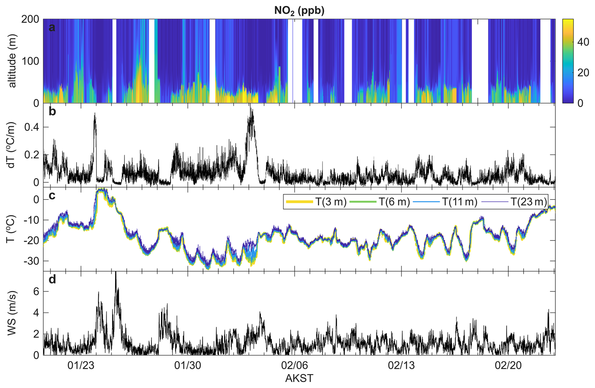
Figure 3 Retrieved vertical profiles of NO₂ (a) compared to temperatures at 3, 6, 11, and 23 m (c) and temperature gradients (b). Wind speeds at 23 m are displayed in panel (d).

The presence of the PSL is associated with low wind speeds (Fig. 3d) and strong temperature gradients (Fig. 3b). Times with increased wind speeds lead to negligible temperature and trace gas gradients, for example on 28 January and 4 February. The increased vertical mixing and wind-driven export during these time periods is responsible for low pollutant levels throughout the lowest 200 m of the atmosphere and the absence of a PSL. During the second half of ALPACA wind speeds were more variable and often reached above 2 m s⁻¹, thus the presence of a PSL becomes less persistent.

3.3 Surface Layer Heights

To better understand how the SLH retrieved from the NO₂ profiles are related to surface temperature inversions in Fairbanks, we performed a statistical analysis of the relationship of SLH and temperature gradients, dT, between 3 and 23 m altitude (Fig. 4a). Lower SLH are clearly associated with larger dT (Fig. 4a). At dT=0.0125 °C m⁻¹ a median SLH of 56 m is found, indicating that even relatively weak temperature gradients can be associated with SLH in the 50 to 60 m range. However, this dT bin also includes conditions where no well-defined PSL is formed. SLH decreases steadily from dT=0.0125 to dT=0.1375 °C m⁻¹ and levels off around 25 m. The variability of the SLH also decreases, implying that strong temperature inversions are always associated with low SLH. It should be noted here that the formation of surface temperature inversions and a PSL are not completely synchronous, as emissions take time to accumulate. We thus expect a certain amount of variability from this effect in our analysis. Nevertheless, it is clear that the SLH is closely related to surface temperature inversions, a result that we will use later when developing a parameterization for surface mixing for PACT-1D.

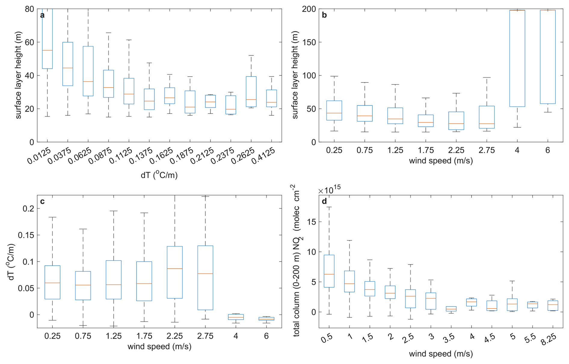
Figure 4 Statistical analysis of the dependence of (a) surface layer height on temperature gradient; (b) surface layer height on 23 m wind speed; (c) surface temperature gradient on wind speed, and (d) NO₂ column density on wind speed.

3.4 Influence of Wind Speeds

Wind speed also impacts the PSL height. SLH below 50 m are only observed when wind speeds are lower than 3 m s⁻¹. For larger wind speeds, no clear surface inversion or inversions above 200 m are found (Fig. 4b).

There are two possible explanations for the influence of wind speed on surface pollution. Larger wind speeds can cause shear-induced turbulence leading to weakening or breaking up of the surface inversion. In fact, non-zero surface temperature gradients are only found for wind speeds below 3 m s⁻¹ in Fairbanks (Fig. 4c), supporting the idea that low wind speeds are a requirement for the formation of the PSL.

Wind also horizontally advects pollution out of and clean air into the Fairbanks urban area, thus lowering pollutant levels. To investigate this, we calculated the 3–200 m column density of NO₂ and SO₂ by integrating our trace gas profiles with altitude. A statistical analysis shows that trace gas columns, i.e. the vertically integrated concentrations, decay with increasing wind speed and reach values close to zero around 3 m s⁻¹ (Fig. 4d), illustrating the effect of advection on air pollution in Fairbanks.

In summary, our analysis seems to indicate that PSL formation only occurs at wind speeds below 3 m s⁻¹, while shear induced turbulence and advection remove surface pollution effectively above wind speeds of 3 m s⁻¹.

4 Modeling of vertical trace gas profiles

4.1 The PACT-1D model

To provide a more quantitative analysis of the processes leading to vertical trace gas profiles in Fairbanks, we set up UCLA's 1D vertical chemistry and transport model PACT-1D (Tuite et al., 2021; Ahmed et al., 2022; Kuhn et al., 2025) to represent the 4 km×4 km area of downtown Fairbanks. PACT-1D is an observation-driven one-dimensional model designed for the interpretation of field observations and mechanistic studies. The model simulates the temporal evolution of trace gas concentrations based on a set of boundary conditions, such as emissions, turbulent diffusivities, wind speed, photolysis rates, and temperature, many of which are constrained by field observations. The model does not constrain trace gas concentrations. The chemical scheme in PACT-1D is based on the RACM2 mechanism (Goliff et al., 2013). The model considers molecular uptake of trace gases on the ground, which, in combination with the transport scheme, leads to deposition (see Tuite et al., 2021, for details). We ran the model for the entire ALPACA period using photolysis frequencies measurements by the Univ. of Houston's spectroradiometer and temperatures and RH from observations at the CTC site (Simpson et al., 2024).

For Fairbanks we use the model with 39 vertical grid cells, of which 32 are in the lowest 200 m and 11 in the lowest 20 m of the atmosphere. Grid spacing decreases towards the surface to capture the fine structure of the PSL. Emissions, vertical eddy diffusivities and horizontal advection are central to accurately describing pollutant concentrations in the PSL. They are also supplied externally to the model, which will be discussed in the following sections.

Pollutant emission rates

Emission rates of pollutants are reported by the Alaska Department of Environmental Conservation, ADEC, with hourly resolution on a 1.33 km regular horizontal grid distributed in 4 vertical grid boxes between 0 and ca. 20 m a.g.l. We spatially average the reported emissions horizontally over a 4 km×4 km area covering the major part of downtown Fairbanks and interpolate their vertical distribution to the PACT-1D grid. We consider all reported surface sources, and neglect the influence of surrounding point sources as their influence is not significant for our study (Albertin et al., 2024; Brett et al., 2025). NO_x emissions in the inventory have been found to be substantially underestimated at cold temperatures due to uncertainties in combustion chemistry (Brett et al., 2025). This is confirmed by our simulations. An adjustment of the ADEC emissions of NO (by a factor of 2.3) and NO₂ (by a factor of 3), aligns well with the suggested correction of 3 for total NO_x for −20 °C by Brett et al. (2025) and results in very good agreement between PACT-1D and our observations, as discussed in more detail in the Supplement (Sect. S3).

4.2 Parametrization of trace gas transport

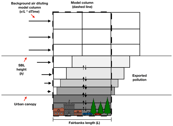
The results of the statistical analysis (Sect. 3.3) can be used to develop a conceptual model of the lower atmosphere in Fairbanks (Fig. 5), which can be translated into a parameterization for inclusion in a one-dimensional model. Our observations show that under conditions of weak surface winds and the formation of a surface temperature inversion, surface emissions accumulate in a shallow PSL (Fig. 3). Dilution of surface layer air with background air thus appears strongly reduced. However, the fact that trace gas concentrations in the surface layer do not continuously increase, often reaching a plateau (Fig. 2), indicates the presence of some residual mixing across the top of the PSL. The small trace gas concentrations above the PSL and the strong gradient at the top of the PSL (Fig. 3) imply that trace gases leaving the PSL are efficiently removed. We attribute this removal to advection by horizontal wind, which is typically stronger above the PSL.

Figure 5 Conceptual model of the dispersion of pollutants in the Fairbanks lower atmosphere.

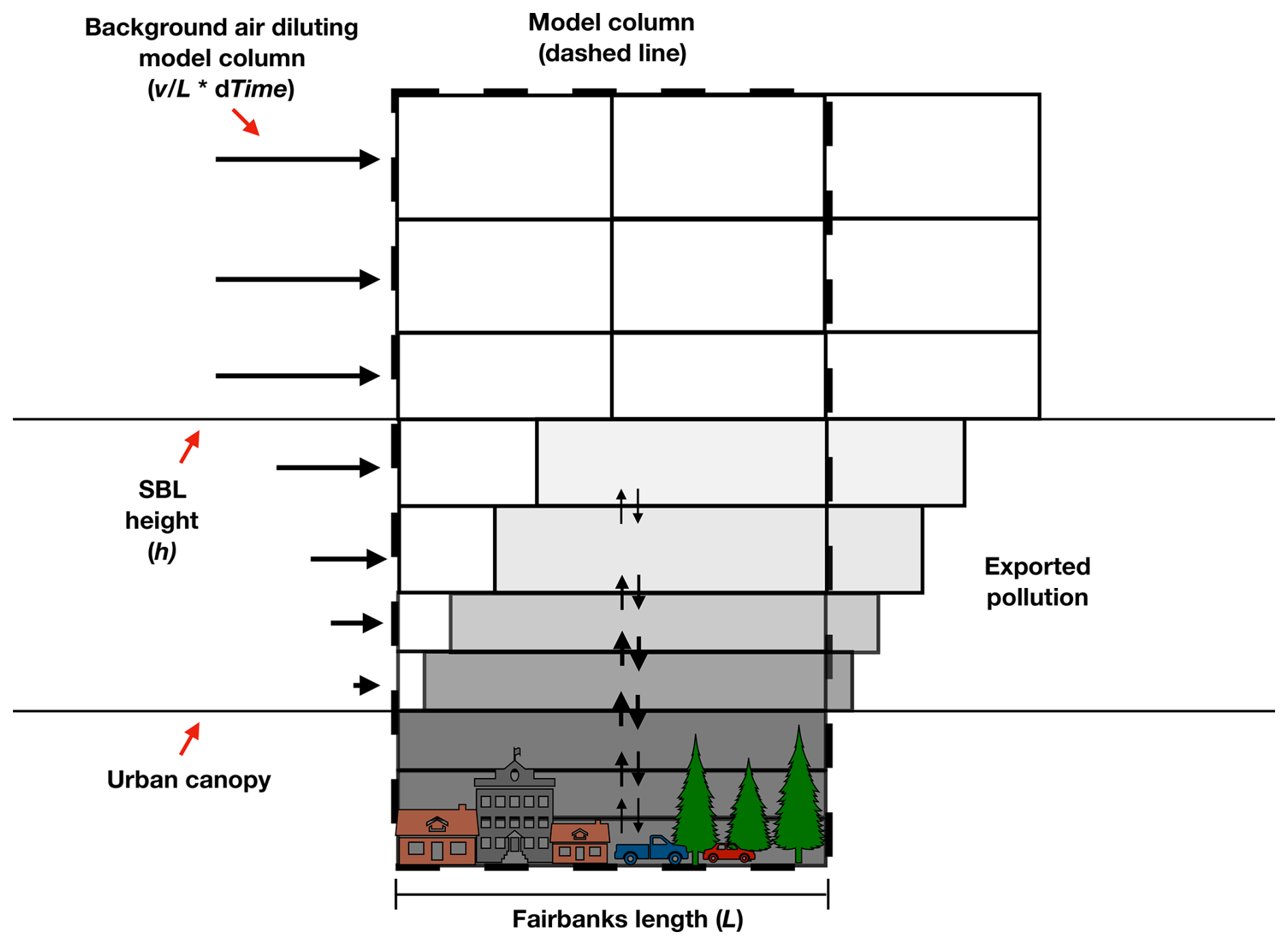
Overall, a picture emerges where, at low wind speeds, emissions accumulate in a shallow surface layer, while slowly being mixed out of the top of the PSL where they are removed by advection (Fig. 5). A pseudo steady state, PSS, between emissions and this loss is often established in the PSL. We will discuss the impact of this PSS and the associated residence times in Sect. 5.4. We can now use this conceptual model to develop a parameterization for vertical mixing and advection loss in our one dimensional model.

4.2.1 Parameterization of vertical exchange

PACT-1D uses a flux-gradient relationship to simulate vertical trace gas transport (Tuite et al., 2021) and therefore requires vertical profiles of eddy diffusivities, K_z(h), as input data. Because direct measurements of K_z(h) were not made in downtown Fairbanks during ALPACA we will use a commonly used empirical parameterization developed by Brost and Wyngaard (1978). This parameterization uses the SLH, H, friction velocity, u^*, the local Obukhov length, L_O, and the von Kármán constant, κ=0.4 to calculate K_z as a function of altitude, z.

$$\begin{array}{}\text{(2)}& K_z\left(z\right)=\mathit{\kappa }{u}^{*}H{\displaystyle \frac{(z/H)(\mathrm{1}-z/H{)}^{\mathrm{1.5}}}{\mathrm{1}+\mathrm{4.7}(z/H)(H/L_{\mathrm{0}})}}\end{array}$$

The main information from our observations is the SLH determined from our trace gas vertical profiles. We interpret the SLH as the height through which turbulent eddies distribute near-surface-emitted pollutants (Fig. 4a). Our definition of the SLH differs from that typically used in meteorology, as it is based on tracer rather than temperature profiles. It is likely that these two heights are different, as trace gas and temperature profiles are established on different length- and time-scales, as we will discuss in Sect. 5.1. In addition, trace gas emissions are limited to the urbanized Fairbanks area, while regional heat fluxes can affect areas inside and outside the urban core. We do not have detailed temperature profiles to investigate this issue further, but we expect that our SLH is smaller than many meteorologically based definitions of surface layer height (Stull, 1988; Anderson and Neff, 2008).

A challenge in using Eq. (2) is that our SLH data has a low time resolution and gaps during times when visibility was too low for the LP-DOAS instrument to collect data. In addition, direct continuous observations of vertical trace gas profiles are very rare, and a direct application of SLH would not provide information for future studies. Consequently, we use the relation of observed SLH to the observed median temperature gradient, dT, between 23 and 3 m at the CTC site (Fig. 4a) to create a lookup table for H as a function of dT for dT>0.0125 °C m⁻¹. For dT<0.0125 °C m⁻¹, we assumed a well mixed atmosphere with a constant K_z=10 m² s⁻¹, large enough to dilute pollution to reflect the vertically integrated observations. Sensitivity studies show that the model results are independent of this choice of H under near-neutral high-wind conditions. H values for a specific model time were then calculated through a linear interpolation between the lookup table entries for dT observed at that time. We use $H/L_{\mathrm{O}}=\mathrm{1.4}$ according to Brost and Wyngaard (1978), who noted that variations in $H/L_{\mathrm{O}}$ had only small effects on the vertical shape and peak of the K_z profiles calculated by Eq. (2). Brost and Wyngaard (1978) list u^* values in the range of 0.25–0.13 m s⁻¹ for their parameterization over flat surfaces. However, the friction velocity is expected to be higher over the rough urban canopy of Fairbanks. Considering typical urban areas roughness lengths (∼1–5 m, Foken, 2008) we estimate that u^* is increased by a factor of 2–3 from the original value in Brost and Wyngaard (1978) and consequently used $u^{*}=\mathrm{0.45}$ m s⁻¹ in our implementation of Eq. (2) in the model. With these assumptions, the K_z profile predominantly depends on the surface layer height, H.

4.2.2 Treatment of horizontal exchange

To account for advective transport we added a horizontal dispersion parameterization to the PACT-1D. This parameterization is based on a horizontal advective exchange with a background atmosphere with the same vertical grid and concentrations typical for a background atmosphere for the most important trace gases. For most gases these values are considerably lower outside the PSL, with the exception of ozone, which was set to 35 ppb. We calculate the horizontal exchange coefficient, K_exch(z) as a function of the wind speed profile at each time step, ν(z), and the length scale, L, following the mass balance approach from Jacob (2000):

$$\begin{array}{}\text{(3)}& K_{\text{exch}}\left(z\right)=\mathit{\nu }\left(z\right)/L\end{array}$$

L=4 km was chosen as a value representing the length of the urban core of Fairbanks. For our model runs describing the ALPACA study we combined WRF-model output and observed wind speeds (Simpson et al., 2024). Weather Research and Forecasting (WRF) model wind speeds for the center of Fairbanks (64.842° N, −147.700° E) were provided by the U.S. EPA. Wind speeds were directly measured at 23 m height at the CTC site and at 2 and 10 m height at the nearby NCore site. Wind speed near the surface were linearly interpolated between the observations at 2, 10, 23 m, and model results at 50 m.

4.3 Model output and diagnostics

One of the advantages of using a detailed 1D model is the ability to archive all relevant chemical reaction rates and trace gas fluxes. Because one of our goals is to understand how trace gas fluxes, J(z), at altitude z impact chemistry, we will use transport rates, i.e. the rate at which transport contributes to a change in concentration at a certain altitude: $\frac{\mathrm{d}{C}_{\text{transport}}\left(z\right)}{\mathrm{d}t}=J_{\text{net}}\left(z\right)/h$ in units of $\mathrm{molec}.{\mathrm{cm}}^{-\mathrm{3}}{\mathrm{s}}^{-\mathrm{1}}$, where J_net is the net flux into or out of the model grid box and h is the box height. When appropriate, we distinguish between vertical transport and advection terms.

Another diagnostic tool we use is the residence time of a trace gas in the PSL (see also Kuhn et al., 2026). A comparison between this residence time and the timescale of chemical reactions provide important insights into the behavior of the chemistry-transport system in the PSL. The residence time is commonly calculated using the assumption of a pseudo steady state, i.e. stationary atmospheric transport conditions. We calculate this instantaneous residence timescale τ^⋆(t) from the modeled vertically integrated pollutant concentration $\overline{c}$, and the transport-related removal rates of pollutants from the PSL (V^† and H^†, where V^† includes deposition). The latter are calculated by integrating vertical and horizontal transport rate profiles, V and H, over the height of the PSL (h_PSL):

$$\begin{array}{}\text{(4)}& {\mathit{\tau }}^{\star }={\displaystyle \frac{\overline{c}}{H^{\mathit{†}}+V^{\mathit{†}}}}={\displaystyle \frac{{\int }_{\mathrm{0}}^{h_{\text{PSL}}}c\left(h\right)\mathrm{d}z}{{\int }_{\mathrm{0}}^{h_{\text{PSL}}}H\mathrm{d}z+{\int }_{\mathrm{0}}^{h_{\text{PSL}}}V\mathrm{d}z}}\end{array}$$

However, the instantaneous residence timescale τ^⋆ does not represent the true residence time of a gas within the surface layer. For example, if at a given time t, τ^⋆ is 3 h but one hour later changes to 1 h, the effective residence time at t will be shorter than 3 h. The effective pollutant residence time τ(t) at a given time t therefore depends on the future value of τ^⋆. The effective residence time is the upper bound of the following integral expression:

$$\begin{array}{}\text{(5)}& \underset{t}{\overset{t+\mathit{\tau }\left(t\right)}{\int }}{\displaystyle \frac{\mathrm{1}}{{\mathit{\tau }}^{\star }\left(t^{\prime }\right)}}\mathrm{d}{t}^{\prime }=\mathrm{1}\end{array}$$

We can solve this equation numerically for τ to thus determine the temporal evolution of the effective residence time τ of pollutants in the PSL (see Sect. 5.4).

4.4 Modeling results

The model results for the entire ALPACA experiment (Fig. 6d–f) reproduce the presence of frequent PSLs observed by the LP-DOAS system (Fig. 6a–c). It accurately captured persistent PSLs, with increased concentrations of SO₂ and NO₂ and depleted ozone, interspersed with periods of efficient mixing and low SO₂ and NO₂, during the first third of the experiment. The model also reproduces the more variable PSL in the second half of the experiment, when increased solar heating leads to more mixing during the day. The height of the modeled PSL is slightly (∼10 m) higher than those observed, but considering the uncertainties in height retrievals and vertical mixing parameterization, the agreement is very good.

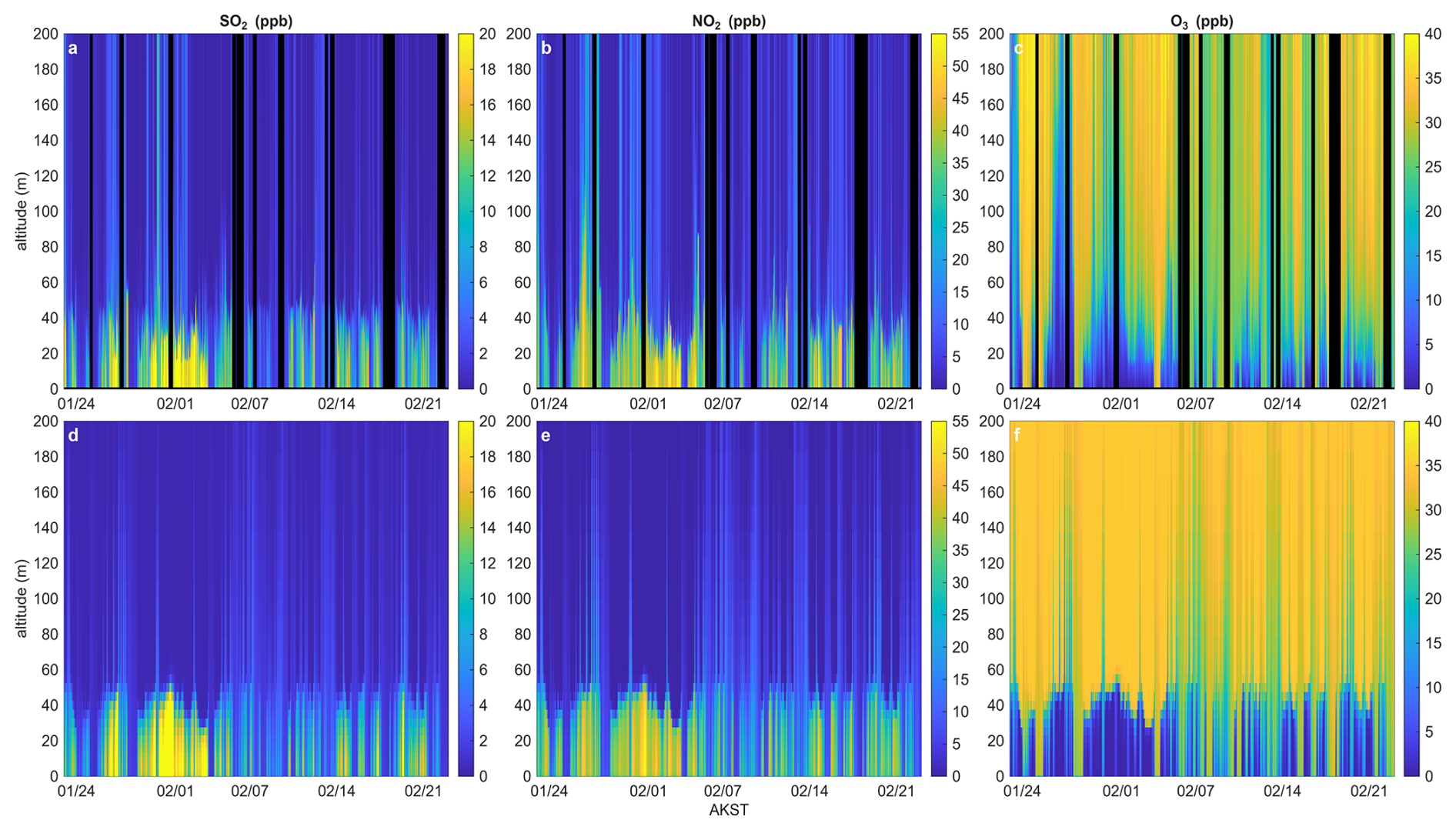
Figure 6 Campaign overview of retrieved (a–c) and modeled (d–f) vertical mixing ratio profiles of SO₂ (a, d), NO₂ (b, e), and O₃ (panels c, f).

Over the entire experiment SO₂, NO₂ and O₃ mixing ratio agree well between model and observations (see Sect. 4.4.1). The opposite profiles of NO₂ and O₃ will be discussed in more detail in Sect. 5.3. During some instances of intermediate mixing, for example when ozone mixing ratios are low throughout the entire 200 m high domain on 26 January and 1 February, the model is unable to correctly reproduce the concentrations aloft. We attribute this to mixing in the model being too weak during these times, pointing to a need to improve our parameterization for these cases. In the following two sections we will provide a more detail look at the model-observation intercomparison of mixing ratios and profile shape.

4.4.1 Comparison of Model and Observations

To better validate PACT-1D without consideration of the potential uncertainties introduced by our vertical profile retrievals, we compare the LP-DOAS observation with model output. The LP-DOAS averages over four different height intervals, therefore we averaged the model output over the same intervals. The comparison for NO₂ (Fig. 7) shows that the model captures the variability of NO₂, which is driven by the interplay of NO_x emissions, conversion of NO to NO₂, and changes in vertical mixing. The fast transition between a PSL and cleaner periods, for example on 28 January and 4 February, are captured exceptionally well in the 12–17 m height interval (Fig. 7a). We observe a similar agreement with O₃, SO₂, HCHO, and HONO (see Figs. S9–S12). Similarly, the model captures the variability on the 17–73 m, 17–115 m and 17–191 m light paths well, reproducing the smoother mixing ratio changes and lower mixing ratios as the interval expands upwards (Fig. 7c, e, and f). The excellent agreement between the direct observations and the model output gives us confidence that our emissions, wind speeds, and the vertical transport parameterization provide a very good description of the atmospheric conditions during ALPACA.

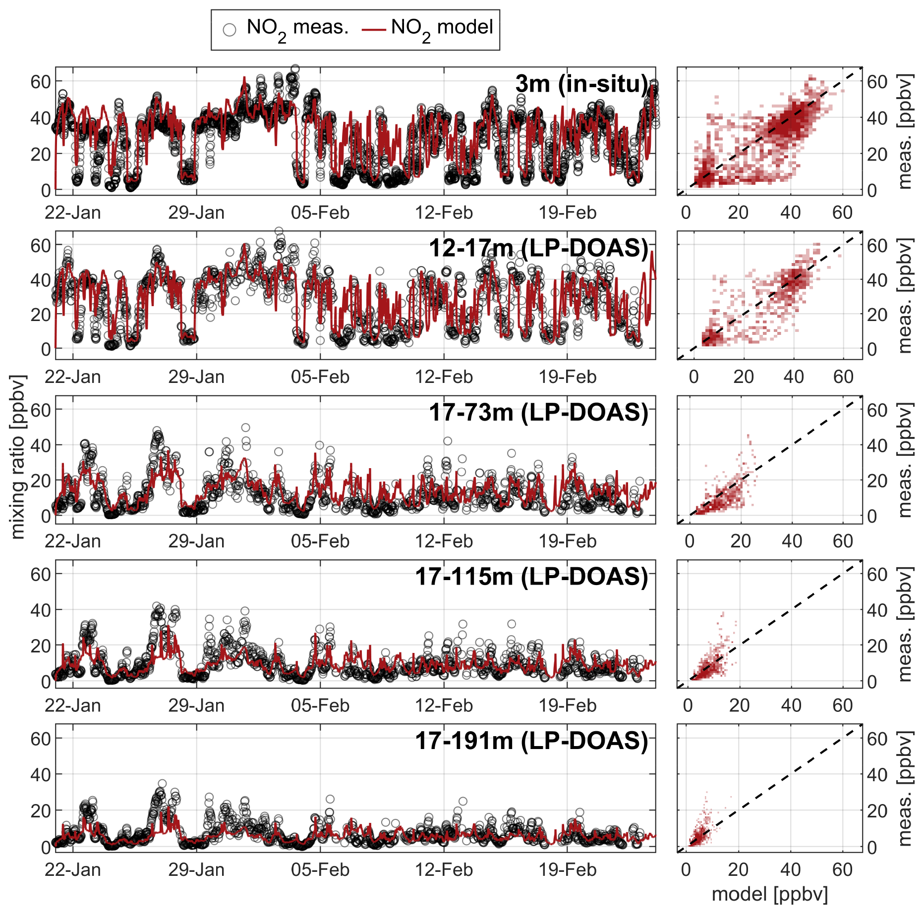
Figure 7 Comparison of in-situ and LP-DOAS observations of NO₂ with model output. The model data for the LP-DOAS comparison was averaged over the same height intervals as the respective light paths. As explained in the text, much of the disagreement between model and observations is due to the challenge of correctly describing the timing of the multiple transitions from polluted to clean conditions. This can clearly be seen in the correlation plots of the in-situ and the 12–17 m data and is reflected in the correlation coefficients (R²=0.54, 0.55, 0.45, 0.44, 0.4, respectively, from top to bottom panels). Comparison plots for the other trace gases can be found in the Supplement (Figs. S9–S12).

The rapid transitions in mixing ratios during ALPACA makes a statistical analysis of the observation-model agreement challenging. Small shifts in timing of a transition, which we can expect solely from the spatial difference of in-situ temperature gradients vs. path-averaged concentrations, will lead to large differences in mixing ratios between model and observations, which then gives the impression of a general disagreement. This effect is particularly visible in the NO₂ correlation plots for in-situ and 12–17 m path observations (Fig. 7b) where, at times, high/low observations coincide with low/high model mixing ratios. We have not accounted for this issue, as such an effort would not add useful information to our analysis.

4.4.2 Modeled vertical profiles

To further investigate our vertical mixing approach and the pollutant emission rates in PACT-1D we compared modeled vertical profiles for times within 5 min of the observations (Fig. 8a–c, f–h, and k–m). The model reproduces the formation of a polluted surface layer on 2 February, with a height that agrees very well with the observations of SO₂ and NO₂ (Fig. 8a and f). Surface SO₂ is smaller in the model than in the observations, most likely due to slightly underestimated sulfur emissions. The agreement for NO₂ is excellent, likely because NO_x emissions were scaled to fit the observations, and NO₂ formation by ozone titration is limited by background ozone. The modeled ozone profile (Fig. 8k) shows a step function that is the inverse of NO₂, which is expected considering the chemistry of this system (Sect. 5.3). The retrieved ozone profile does not show an abrupt transition from the surface layer. This can be explained by the uncertainty in the retrieval (ozone observations have higher uncertainties compared to SO₂ and NO₂) as reflected by the shaded area in Fig. 8k.

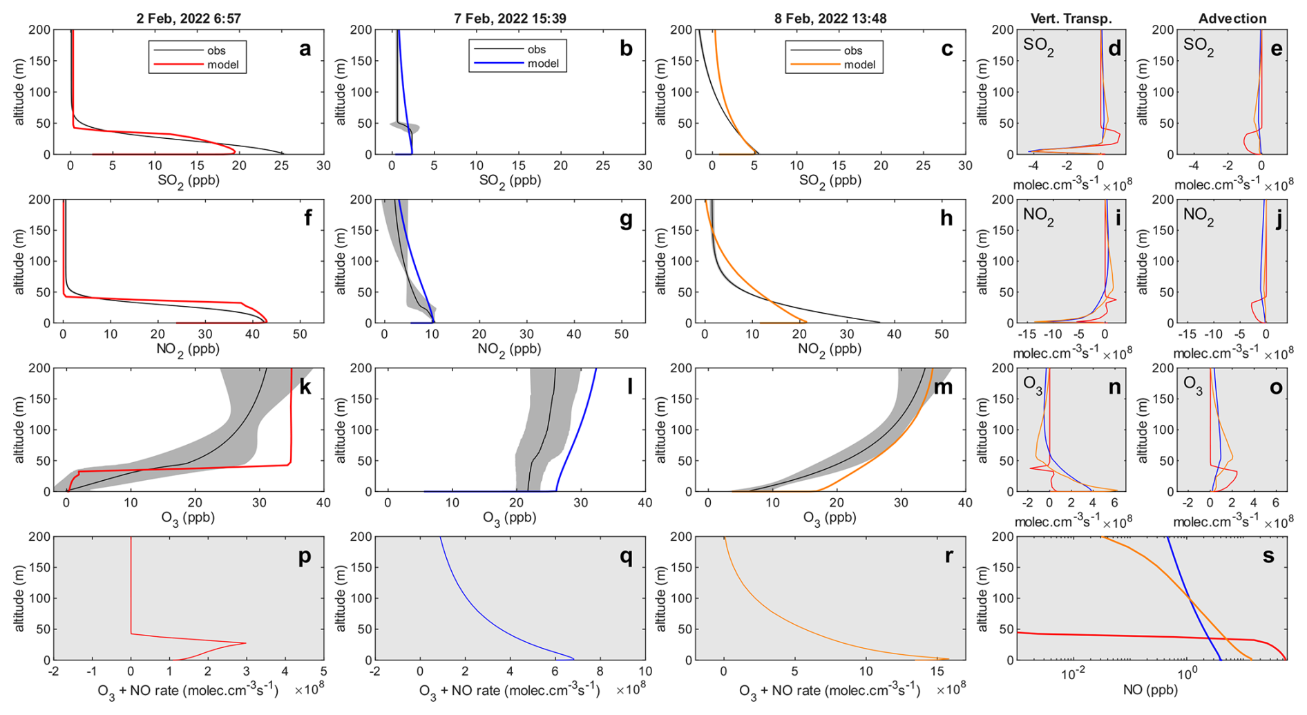
Figure 8 Examples of retrieved and modeled vertical mixing ratio profiles of SO₂, NO₂, and O₃. The shaded area shows the profile uncertainty due to the measurement error. Shaded panels on the right depict the modeled vertical and advective transport rates of SO₂ (d, e), NO₂ (i, j), and O₃ (n, o). The bottom three panels (p–r) show the vertical profiles of the O₃+NO reaction rate for the three examples, where the respective NO vertical profiles from the model are shown in panel (s).

Agreement between the modeled and retrieval profiles on 7 February is also very good (Fig. 8b, g, and l). The SO₂ and NO₂ profiles show a small transition at around 30 to 40 m that is not reflected in the model, caused by a small jump in our eddy diffusivities at this altitude. Considering that the profile shapes are very similar between model and observations, the small difference in the mixing ratios across the profiles are likely due to the uncertainties in the emissions. Similarly, the profile shape on 8 February generally agree well for SO₂ (Fig. 8c, h, and m). NO₂ and O₃ mixing ratios at the surface differ by ∼15 ppb in opposite direction on 8 February due to a small underestimate of NO emissions, which propagates through the profile.

The excellent agreement of the observed and modeled vertical profiles supports the choice of a sigmoidal function for our retrievals and the transport parameterizations in PACT-1D. The trace gas emissions in PACT-1D seem to have small inaccuracies that do not impact the ability of the model to reproduce the behavior of the vertical trace gas distribution in the Fairbanks lower atmosphere. We can thus use both the retrieved profiles as well as the model outputs to further analyze the chemistry and transport processes controlling air pollution in Fairbanks.

5 Discussion

Our combined observations and model results offer a unique opportunity to investigate various phenomena observed in the Fairbanks winter atmosphere. In the following sections we will focus on transport and gas-phase related topics. Detailed implications for multiphase chemistry, which are beyond the scope of this study, are discussed in Kuhn et al. (2026), who show that vertical mixing and transport has a substantial impact on oxidation chemistry and aerosol composition. For example, the diurnal profile of aerosol nitrate is due to the competing effects of chemical formation and transport loss. These results also show that the contributions of aerosol chemistry to the budget of the trace gases discussed here are minor and do not impact our main conclusions.

5.1 Timescale of Polluted Surface Layer Formation

An interesting observation during ALPACA was the rapid formation of the PSL. A close look into the morning hours of 4 February shows that before 02:15 AKST, in the absence of a temperature inversion (Fig. 9f) ozone was relatively well mixed in the lowest 200 m of the atmosphere, as shown by the agreement of the in-situ and LP-DOAS measurements (Fig. 9d). Similarly, SO₂ showed a weak vertical profile, with 2 ppb at the surface and 0.3 ppb on the upper LP-DOAS light path. Once the temperature inversion starts to form, around 02:15–02:30 AKST, surface SO₂ increases (Fig. 9e) and surface ozone decreases (Fig. 9d). SO₂ in the 12–17 m height interval follows the 3 m in-situ data. In contrast, O₃ in the 12–17 m interval showed a 20 min delay and ozone mixing ratios remained larger after 04:00 AKST when the 3 m data was close to zero. In-situ NO starts increasing considerably later than SO₂ and only appears when ozone has been nearly completely depleted at the surface (Fig. 9d). The LP-DOAS observations of SO₂ and O₃ on the three light paths above 17 m, on the other hand, showed little change, indicating that the PSL was confined to the lowest 20 m of the atmosphere.

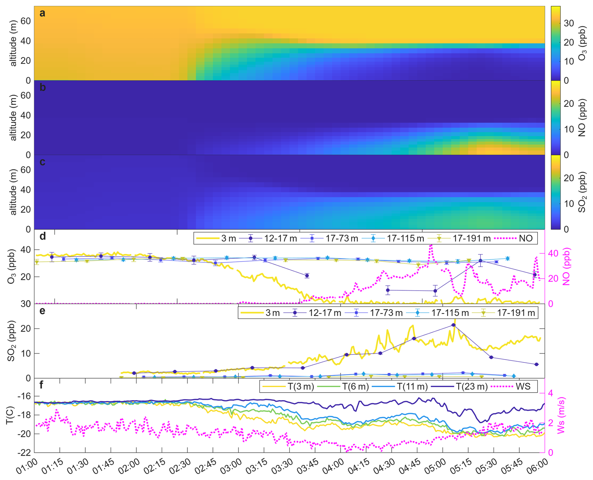
Figure 9 Formation of the PSL on 4 February 2022. The top three panels (a–c) show the model results for this event. Panel (d) shows the path-averaged LP-DOAS and in-situ ozone data (left y axis) and the surface NO data (magenta, right y axis). The light path above 17 m height shows a constant O₃ mixing ratio of ∼35 ppb, while the PSL mixing ratios drop at the onset of the event at around 02:45 AKST. Panel (e) shows the observations of SO₂ for LP-DOAS and in-situ data. The PSL observations of the two instruments agree very well, and also show an increase in SO₂ during this event. Temperature gradients (panel f, left y axis) form around 02:15 AKST, during a time when the wind speed (magenta, right y axis) is around 2 m s⁻¹.

The model results (Fig. 9a–c) generally agree with the observations and clearly show that ozone depletion at the surface occurs from the ground upwards, as NO surface emissions first react with surface O₃. As ozone is depleted at the surface and NO accumulates, vertical mixing of NO will cause ozone destruction higher up in the PSL. The non-zero 12–17 m ozone mixing ratios around 04:45 AKST indicate some residual ozone in the upper part of the PSL. This is supported by the model which shows ozone at the top of the PSL, albeit at a somewhat larger height than the observations. The high 12–17 m ozone mixing ratios after 05:00 AKST are not reproduced by the model and could indicate that the PSL height decreases below 12 m, or due to some mixing at the top of the PSL. Interestingly, the high ozone coincides with decreasing SO₂ at the surface and at 12–17 m. Vertically more highly resolved measurements are required to study such cases in the future.

5.2 Profile shape

Surface pollution in wintertime Fairbanks is associated with the formation of a PSL, as clearly illustrated by the direct profile observations shown in Fig. 6. Here we discuss this dependence by analyzing three distinct vertical trace gas profile scenarios.

The first scenario corresponds to a strongly polluted PSL. It is characterized by a shallow PSL with high concentrations of primary pollutants, such as SO₂ and ${\mathrm{NO}}_x=\mathrm{NO}+{\mathrm{NO}}_{\mathrm{2}}$, and low ozone. Figure 8a, f, and k shows an example of such a profile from 08:13 AKST on 2 February 2022. The observed and modeled profiles of SO₂ and NO₂ show a remarkable near step-wise transition from a highly polluted surface layer with 28.4 ± 1.1 ppb of SO₂ and 45 ± 0.7 ppb of NO₂ to background air with low mixing ratios. Defining the height of the layer as the halfway point between surface and 200 m mixing ratio yields ≈34 ± 7 m for SO₂ and 43 ± 5 m or NO₂. The retrieved ozone profile shows a slightly smoother shape with 1 ± 5 ppb at the surface and 35.2 ± 5 ppb at 200 m altitude. While the shape is different from that of the other two trace gases, the height of the half-way-point is similar, at 34 ± 15 m. As the shaded areas representing the uncertainty (Fig. 8) show, our profile retrieval can only identify the surface-layer height to within 5 to 10 m for SO₂ and NO₂ and is even less accurate for ozone.

The abrupt transition in the SO₂ concentration profiles is a common phenomenon during PSL events (see also Fig. 6). In our model this transition is caused by a drop of K_z to very low values at the transition height and increased advection above the transition. The modeled vertical transport and advection rates expressed as the rate of concentration change due to the respective transport process in each box in Fig. 8d and e (red curves) show a negative vertical transport rate below ∼20 m and a positive rate between 20–40 m, indicating that freshly emitted SO₂ is transported into the upper part of the PSL. A small amount of SO₂ is also advected out of the urban core. In the 20–40 m height interval upward transport and advection balance each other, making advection the main SO₂ loss process. A similar picture emerges for NO₂ (Fig. 8i and j, red curve). The region of loss due to vertical transport is lower in the PSL due to traffic emissions occurring closer to the ground. The vertical gradient of NO₂ is less pronounced in the PSL than that of SO₂, due to its chemical formation through the NO+O₃ reaction. The loss of NO₂ from the PSL thus occurs predominately at the top of the PSL as indicated by the small positive vertical transport rate peak (Fig. 8i). Advection of NO₂ is similar to that of SO₂.

Mixing ratio profile and transport rates for ozone are generally inverted from those of NO₂, except for the surface peak which stems from NO₂ emissions (Fig. 8n and o, red curve). The downward transport of ozone thus also occurs primarily at the upper part of the PSL, where there is a transition from a weakly positive to a negative peak of the transport rate.

Our second scenario is that of a well-mixed atmosphere, such as that encountered at 15:39 AKST on 7 February 2022 (Fig. 8b, g, and l). SO₂ and NO₂ mixing ratios are much smaller at the surface, at 3 and 12 ppb respectively, while they seem slightly higher aloft than in our first scenario. The reverse behavior is true for ozone with modeled mixing ratios of 25 ppb at the surface and 32 ppb aloft. The fact that ozone mixing ratios at 200 m are lower than the model background of 35 ppb and the presence of 0.5 ppb of NO aloft (Fig. 8s) indicates that ozone is titrated by NO emissions (which peak during that time of day) throughout the lower atmosphere. The vertical transport rate profiles reflect this behavior with negative values below ∼20 and ∼50 m for SO₂ and NO₂, respectively, and positive rates above (Fig. 8d and i, blue curve). Ozone vertical transport is the inverse of that of NO₂ (Fig. 8n, blue curve). The transport rates are generally larger than in the polluted scenario due to enhanced turbulent mixing.

Our third scenario is an intermediate case when the atmosphere is stable but a distinct surface layer is not formed, such as at 13:48 AKST on 8 February 2022 (Fig. 8c, h, and m). This case shows pronounced vertical profiles and increased surface mixing ratios of SO₂ and NO₂ and low, but non-zero, ozone mixing ratios. These profiles are more similar to those previously observed in lower-latitude urban areas at night (Wong et al., 2011; Tuite et al., 2021). The vertical transport rate profiles in this case are similar to our second scenario, but generally more pronounced (Fig. 8d, i, and n, orange curve).

5.3 The role of NO titration by O₃ in determining PSL chemistry

One of the most visible consequences of the presence of the urban PSL are the low ozone mixing ratios at the surface and the extremely strong ozone vertical concentration gradient across the top of the PSL, which are accompanied by the inverse gradients of NO₂. This phenomenon, and the generally inverted profiles of O₃ and NO₂, can be explained by the emission of NO, reaction of NO with ozone and the very slow entrainment of ozone rich air from the background atmosphere aloft and by advection. Modeled NO profiles (Fig. 8s) show very high surface mixing ratios during strong PSLs, in good agreement with the observations. Modeled NO mixing ratios above the PSL are very low in this case. NO profiles also show the same abrupt transition as the other PSL pollutants. As the Fairbanks atmosphere becomes more mixed the NO mixing ratios and the concentration gradients weaken.

We extracted the $\mathrm{NO}+{\mathrm{O}}_{\mathrm{3}}\to {\mathrm{NO}}_{\mathrm{2}}+{\mathrm{O}}_{\mathrm{2}}$ reaction rates from the model to illustrate how ozone chemistry changes for the three stability regimes (Fig. 8p, q, and r). In the case with a strong PSL (Fig. 8p) the reaction rate increases in the PSL to a maximum of $\sim \mathrm{3}\times {\mathrm{10}}^{\mathrm{8}}$ $\mathrm{molec}.{\mathrm{cm}}^{-\mathrm{3}}{\mathrm{s}}^{-\mathrm{1}}$ near the top of the PSL where NO and background ozone mix.

In scenarios with more mixing, and larger ozone surface mixing ratios, the $\mathrm{NO}+{\mathrm{O}}_{\mathrm{3}}\to {\mathrm{NO}}_{\mathrm{2}}+{\mathrm{O}}_{\mathrm{2}}$ reaction rate increases from the ground upwards. Interestingly, small amounts of NO and therefore reaction rates can be found up to 200 m altitude in these cases (Fig. 8s). Our results show that increased mixing leads to more pronounced profiles of the reaction rate and more NO aloft.

5.4 Residence time

The common view of the role of the PSL in air quality is that it “traps” pollution. To investigate this perspective more quantitatively, we calculated the effective residence time of pollutants, τ, using the model analytics of an inert tracer, which is emitted into the PSL and transported according to the turbulence-advection scheme (Sect. 4.3).

The effective residence time in the lowest ∼20–50 m during ALPACA is between 0.2 h, when no PSL is present, to 4 h with a well-developed PSL (Fig. 10c). It is closely associated with surface temperature gradients and wind speed (Fig. 10b), confirming the role of surface inversions and advection in controlling PSL mixing with background air (see Sects. 3.3 and 3.4). The effective residence time correlates well with SO₂ mixing ratios (Fig. 10a). This is due to continuous SO₂ emissions, predominantly from residential heating. An analysis of the SO₂ budget reveals that turbulent mixing and advection are the dominant processes controlling SO₂ (and other trace gas) concentrations, while chemical loss and deposition of SO₂ account for less than 10 % of the total budget in our case and thus are of lesser significance. SO₂ is indeed trapped in the PSL, however, in most cases only for 1–4 h.

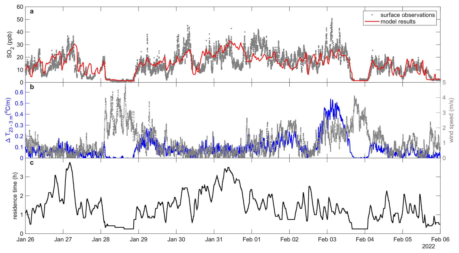
Figure 10 Observed and modeled SO₂ (a) shows the variability imposed by PSL transport processes, which are associated with surface temperature gradients and wind speed (b, shown after applying a 15 min running average). The residence time determined from the model (c) shows low values at times of wind speeds exceeding 2 m s⁻¹. Residence times of 1 h or longer are associated with the presence of temperature inversions.

The range of values of τ have important implications for PSL chemistry. Chemical reactions with a time scale much smaller than τ will proceed completely within the PSL. For example, the average ozone lifetime in a well developed PSL (29 January to 3 February) due to its reaction with surface emitted NO is less than 15 min. The chemical lifetime of NO in the PSL, which is dominated by the NO+O₃ reaction, is somewhat larger but still smaller than τ. Processing of both trace gases therefore proceeds largely inside the PSL. On the other hand, chemical lifetimes of SO₂ and NO₂, for example due to their oxidation by OH radicals, are longer than 100 h. Their PSL concentrations are thus controlled by the efficiency of transport out of the PSL.

Residence times between 1 and 4 h for the extreme cold event shown in Fig. 10 reveal that the PSL is not a permanent trap for pollutants. Pollution is lost by continuous mixing with background air, albeit slowly, and replenished by emissions, even in very persistent PSLs such as those in Fairbanks. The short (1–4 h) pollutant residence times near the surface also limit the formation of secondary aerosol species through multiphase chemistry, because particulate matter is exported from the PSL by the same transport processes. The substantial influence of the short pollutant residence time on PSL oxidation and multiphase chemistry is analyzed and discussed in Kuhn et al. (2026).

6 Conclusions

Severe wintertime pollution events in urban areas are often associated with the formation of a shallow polluted surface layer (PSL). During the ALPACA experiment in winter 2022, we performed continuous LP-DOAS measurements and derived vertical trace gas profiles using a new retrieval algorithm. These highly vertically and temporally resolved profile observations revealed that under subarctic conditions in Fairbanks, AK, the height of the PSL is frequently only 20–40 m. During the coldest periods of ALPACA, at the end of January and beginning of February, the PSL persisted for a period of six days, when some of the highest primary pollutant mixing ratios were observed, i.e. SO₂ up to 35 ppb, NO₂ up to 60 ppb, HONO up to 2.5 ppb, and HCHO up to 7 ppb. Ozone was depleted in the PSL due to its reaction with surface emitted NO. The PSL was less persistent in the later part of February when increasing solar radiation leads to more daytime surface heating and vertical mixing. The unique data set created by our LP-DOAS observations during ALPACA shows the continuous vertical distribution of trace gases during the most polluted periods in downtown Fairbanks. LP-DOAS provides a unique automated observational approach that can be used to further study and monitor this phenomenon. Future deployment of this system to study wintertime PSL would benefit from more light paths inside and at the top of the PSL to further improve the representation of the vertical profiles.

Most previous studies on this topic have correlated meteorological observations with higher surface pollution levels. However, the height of the PSL was determined based on temperature profiles and the measured trace gases were limited (Lareau et al., 2013; Largeron and Staquet, 2016; Hallar et al., 2021). Tethered balloon observations in a field at the outskirts of Fairbanks during ALPACA show surface temperature gradients in the same range as those reported here, but, due to the lack of direct surface emission, the PSL is less well developed (Pohorsky et al., 2025). The balloon-borne observations, while vertically better resolved than ours, provide snapshots in time and do not allow a full analysis of PSL formation, persistence, decay, and the diurnal trace gas cycle. The data presented in our study is, to our knowledge, the first continuous dataset of highly temporally resolved vertical trace gas profiles in a high-latitude wintertime urban area.

Our observations show that the PSL in downtown Fairbanks forms when wind speeds are below 3 m s⁻¹. Pollution levels are much lower above this wind speed, confirming previous reports that link high pollution levels with low windspeeds (Tran and Mölders, 2011). The height of the PSL is linked to temperature inversion strength in the lowest 25 m of the atmosphere. We explore this relationship to develop a conceptual model of PSL mixing. A combination of slow mixing into and out of the PSL and advection aloft explains the loss of pollutants emitted at the surface. Implementation of this conceptual model as an observation-driven parameterization into our 1D chemistry and transport model, PACT-1D, yields excellent agreement with the field observations. This model agreement shows that an accurate representation of vertical mixing and lateral advection, achieved with meter-scale vertical grid spacing, is needed to describe the pollutant concentrations and chemistry in the PSL in Fairbanks. The need to parameterize mixing points to an unresolved challenge of quantifying mixing under stable wintertime conditions (Mahrt, 2014; Hallar et al., 2021). Further work is needed to provide this capability from (micro)-meteorological models to develop air quality modeling results of the same quality as our results. Our results also indicate that air quality models suitable for wintertime Fairbanks need to be able to resolve the vertical extent of the PSL, i.e. use grid spacing in the range of 1–3 m near the surface.

PACT-1D allows a detailed analysis of the coupled chemistry and transport processes leading to high pollution levels in Fairbanks winter. The observed pollution levels are dominated by surface emissions in Fairbanks, such as from traffic and residential heating. This implies that air quality improvement efforts in wintertime Fairbanks should focus on these surface sources, for example by reducing the sulfur content in heating oil to decrease SO₂ and primary sulfate aerosol emissions. The model also points to challenges in the direct interpretation of surface trace gas concentrations with respect to their atmospheric chemistry. Because vertical mixing dominates pollution amounts and formation of the PSL in Fairbanks, temporal trace gas concentration variations need to be interpreted considering both mixing and chemistry timescales. Pollutant residence times in the PSL are on the order of 1–4 h, thus chemical processes proceeding on similar timescales need to consider precursor emissions and reactant removal through mixing. This will be further discussed in the context of secondary aerosol formation in Kuhn et al. (2026). The trace gas concentration plateaus in the PSL are a sign of a balance between emissions, chemistry, and trace gas loss, rather than a temporally static trace gas mixture. This dynamic view of pollutant behavior in the PSL can aid in providing Fairbanks stakeholders with tools and insights to model and mitigate wintertime air pollution.