Estimating Twomey forcing sensitivity to aerosol plume spreading rates

The amount of sunlight that reaches Earth's surface can be reduced by increasing cloud droplet number and decreasing droplet size (i.e., Twomey forcing), a central idea underpinning the Marine Cloud Brightening strategy. Cloud albedo depends nonlinearly on cloud droplet concentration, meaning the spatial extent of aerosol plumes could be an important constraint on the brightening potential. In this study, horizontal aerosol spreading is simulated using a Langevin particle model driven by a library of realistic, 2 d Large Eddy Simulations (LES) spanning the meteorological and aerosol phase space of northeast Pacific stratocumulus. The 2D reflectance fields from the LES are superimposed onto the 2D perturbed aerosol concentrations to calculate the 2D Twomey forcing response.

The Day 1 and Day 2 LES regimes have distinct meteorological, aerosol, and turbulence characteristics associated with equatorward movement of the LES domain. Our results indicate that the Day 2 regime has substantially faster plume spreading than Day 1, with ensemble median differences exceeding 2 km h⁻¹. Despite these differences, Twomey forcing is insensitive to the natural variability in spreading rate. This study suggests that Twomey forcing is resilient to variations in meteorology, aerosols, and turbulence, with its efficacy governed primarily by aerosol lifetime and assumptions surrounding cloud adjustments. Although the natural variation in spreading rate does not materially affect Twomey forcing, idealized plume spreading simulations suggest that current GCM assumptions of an infinitely fast spreading rate could lead to a 10 %–200 % overestimation of cooling.

1 Introduction

In perturbed aerosol conditions, such as freshly emitted ship tracks or theoretical Marine Cloud Brightening (MCB) deployments, the Twomey effect can reduce the amount of sunlight that reaches Earth's surface by producing more, smaller droplets for a fixed liquid water path, acting as a cooling agent in the climate system (Twomey, 1974, 1977; Latham, 1990). In both ship tracks and MCB scenarios, the aerosols are emitted from point sources that spread laterally and vertically over time, with the spatial distribution of the aerosol concentration being an important control on the brightening potential (Twomey, 1977; Wood, 2021). The horizontal spreading of marine boundary layer aerosol plumes has received little attention in the literature (Hernandez-Jaramillo et al., 2025), with only a few studies in recent decades exploring horizontal spreading rate variability and behavior (Durkee et al., 2000; Wang et al., 2011; Berner et al., 2015; McMichael et al., 2024; Prabhakaran et al., 2024; McMichael et al., 2025). In previous explorations of MCB feasibility and regional impact studies (Jones et al., 2009; Rasch et al., 2009; Hirasawa et al., 2023, 2026), global climate models (GCMs) used uniform subgrid aerosol concentrations, making the implicit assumption of an infinitely fast spreading rate. Provided the non-linear Twomey forcing behavior as a function of concentration, the potential consequences of infinite spreading rates in GCMs could be non-trivial. Recently, kilometer-scale regional simulations of ship tracks have enabled explicit representation of some aspects of plume spreading (Tippett et al., 2026). Although these models currently overestimate cooling (Tippett et al., 2026), they remain a promising tool for constraining Twomey forcing.

The in-plume cloud droplet concentrations, which can impact cloud properties such as liquid water path (LWP) and cloud fraction, are not solely a function of horizontal and vertical plume spreading. Cloud droplet activation processes are highly dependent on the aerosol size, number, vertical velocity, and supersaturation (Abdul-Razzak and Ghan, 2000; Wood, 2021). The relationship between cloud droplet concentrations and cloud evolution (aerosol-cloud-radiation interactions) has been a topic of extensive research over the past several decades and remains one of the leading sources of uncertainty in estimates of climate sensitivity (Bellouin et al., 2020). LES explorations of individual ship tracks have suggested that precipitating, clean background aerosol cases augment cooling efficiency through increases in LWP and cloud fraction, with more polluted conditions having smaller, or even negative cloud adjustments (Chun et al., 2023; Prabhakaran et al., 2024).

When trying to constrain cloud adjustments from observations, separating the confounding influence of meteorological variability from the cloud responses to aerosols represents a major challenge (Goren et al., 2025; Gryspeerdt et al., 2016; Stevens and Feingold, 2009). After attempting to control for meteorological variability, several studies find that radiative forcing changes driven by cloud adjustments are relatively weak compared to the Twomey forcing (Tippett et al., 2024; Diamond et al., 2020; Christensen et al., 2026). In contrast, Goren et al. (2026) found that after accounting for cloud morphology, Twomey forcing and cloud adjustments can offset one another, highlighting the potential importance of targeting MCB to focus on the most susceptible cloud regimes. Cloud adjustment sensitivity often diverges between precipitating and non-precipitating environments (Glassmeier et al., 2021). However, cloud buffering mechanisms such as the cloud-radiation-turbulence-entrainment feedback have the theoretical potential to limit such sensitivity (Stevens and Feingold, 2009; Zhu et al., 2005; Wood, 2012). This study does not explore cloud adjustments and makes the assumption that the Twomey forcing is the dominant radiative component; nevertheless, cloud adjustments remain a critical knowledge gap in the estimation of MCB forcing from both simple and sophisticated modeling frameworks.

Beyond the aerosol concentration variability driven by plume spreading, the population of particles available for both transport and activation is governed by the aerosol lifetime, which is modulated by processes such as wet/dry scavenging, entrainment sources/sinks, sedimentation, and coagulation. In precipitating clouds, coalescence scavenging has been shown to be the dominant mechanism determining aerosol lifetime (Wood, 2006), but GCMs show a wide spread in the relative importance of various dry and wet deposition mechanisms (Textor et al., 2006). There have been relatively few attempts to estimate aerosol lifetimes with prognostic aerosol-enabled LES, but Chun et al. (2023) found that the e-folding timescale of 205 nm dry diameter ammonium sulfate aerosols in non-precipitating cases may be 2–3 d, which is substantially longer than the few hours estimated from observations of ship tracks (Glassmeier et al., 2021). In this work, we probe the sensitivity of Twomey forcing to a range of aerosol lifetimes.

The horizontal spreading of aerosols injected from a point source into the marine boundary layer can be reasonably modeled by Langevin particle models (LPMs) (Stohl et al., 2005; McMichael et al., 2024), which depend on turbulence characteristics (i.e., variances and dissipation rates) and precipitation rates, since precipitating boundary layers have been shown to initiate spread-accelerating two-cell mesoscale circulations in large-eddy simulations (LESs) (Prabhakaran et al., 2024; McMichael et al., 2024, 2025). Since LES explicitly resolves much of the energy-containing motion within the boundary layer, velocity variances and dissipation rates are directly accessible from the resolved flow field. These turbulence fields can be used to simulate point source injections in a turbulence environment that originally did not contain aerosol perturbations. In cases where the interaction between the plume and turbulence is strong, such as precipitating boundary layers, the particle model is able to capture the impacts of spread-accelerating mesoscale features using only domain-averaged input parameters through a change in the precipitation-dependent free parameter (C₀). The turbulence information that drives the Langevin particle model, along with background aerosol concentrations, boundary layer depth, precipitation rates, and cloud reflectance fields are derived from a library of realistic, 2 d LES cases based on Lagrangian trajectories, designed to span the meteorological and aerosol phase space of northeast Pacific stratocumulus.

The following analysis is restricted to a subset of the full LES library (54 simulations), focusing on the cloudy LES cases (17 simulations with median cloud fraction > 50 %) that most closely match satellite observations of reflected shortwave energy and represent likely candidate environments for MCB. Additionally, the LPM has not been thoroughly tested in low cloud fraction or cumulus boundary layers. The purpose of this research is to characterize the spreading rate behavior in these cloudy boundary layers across a range of environments and determine how differences in spreading rate, macrophysics, and microphysics may impact the Twomey forcing. In order to do this, the 2D reflectance fields from the LES are superimposed on the 2D aerosol concentrations simulated by the Langevin particle model to calculate the Twomey forcing in each LPM grid column. Given the non-linear dependence of cloud albedo on cloud droplet concentration, variations of spreading rates, cloud morphologies, boundary layer depths, and background aerosol concentrations may lead to complex responses of the Twomey forcing.

To date, plume spreading explorations have been limited to a few idealized LES cases, non-overlapping plumes, and 1–3 d simulation times. The computational effectiveness of the Langevin particle model allows for an exploration of a range of ship track densities, motion, and organization that would be difficult to replicate with LES. This work represents a natural extension of Wood (2021), where cloud morphologies and environmentally dependent spreading rates are now taken into account. Additionally, this study examines the sensitivity of Twomey forcing to aerosol lifetime (Sect. 3.3), injection timing, and duration (Sect. 3.4). The Twomey forcing is decomposed into contributions from particles of different age groups, as well as different aerosol concentration bins (Sect. 3.5). We discuss potential impacts of plume spreading assumptions in GCMs and develop a plume spreading parameterization that could be of use for global modelers (Sect. 3.6 and 3.7).

2 Methodology

2.1 Large-eddy simulation library

Erfani et al. (2025) developed a methodology to explore the meteorological and aerosol phase space of northeast Pacific (NEP) clouds by analyzing eight primary cloud-controlling factors from the European Center for Medium-Range Weather Forecasts (ECMWF) reanalysis version 5 (ERA5) along 2 d Lagrangian trajectories during summer 2018–2021 from six source locations (source locations shown in Fig. 1d). The factors were the trajectory mean 700 hPa water vapor mixing ratio, 700 hPa vertical velocity in pressure coordinates, estimated inversion strength (EIS), and 10 m wind speed, along with the corresponding changes (end minus beginning) in each variable over the trajectory. After performing principal component analysis on 1663 Lagrangian trajectories, Erfani et al. (2025) showed that the first two principal components (PC1 and PC2) explain 43 % of the variance in the cloud controlling factors. At each of the six source locations, 9 trajectories spanning the PC1–PC2 phase space were also shown to reasonably capture the observed variability in surface pressure, liquid water path (LWP), droplet concentrations (N_d), background aerosol concentration (N_a), boundary layer depth, and precipitation (Erfani et al., 2025).

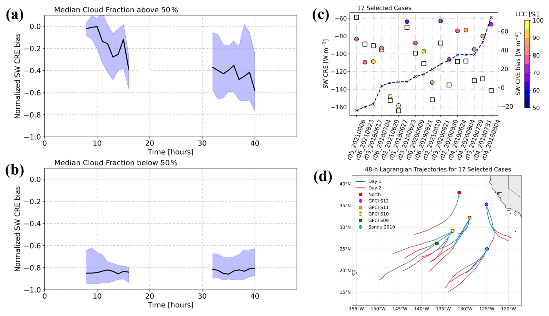
Figure 1 Large eddy simulation library comparison with CERES observations of shortwave cloud radiative effects (SWCRE). (a) The normalized SWCRE bias between CERES and the LES simulation, calculated as SWCRE bias = (LES SWCRE − CERES SWCRE) $/$ CERES SWCRE) with a negative normalized bias indicating that the LES scenes are less reflective than the observations. The blue shaded region is the IQR and the black line is the median for cases with median cloud fraction above 50 % for the duration of the simulation, (b) the normalized SWCRE bias for cases with median cloud fraction below 50 %, (c) raw values of SWCRE from each of the 17 cloudy LES cases (circles) and from CERES (squares) averaged over the 2 daytime periods, with the circle color corresponding the 48 h averaged low cloud cover percentage and the dashed line showing the SWCRE bias (axis on the right, with positive values indicating an underestimation of SWCRE), (d) the cloudy LES domain trajectories for Day 1 in blue and Day 2 in red.

All 54 simulations were carried out with the System for Atmospheric Modeling (Khairoutdinov and Randall, 2003), version 6.10.9, with the same model configuration outlined in Erfani et al. (2025) that is enabled with a two-moment, prognostic aerosol scheme (Berner et al., 2013). Initial ERA5 temperature and moisture profiles required an inversion sharpening procedure to better align with microwave LWP observations and compensate for the coarse representation of inversion structure in ERA5 (Erfani et al., 2022, 2025). During a 12 h, nocturnal spin-up period, temperature and moisture nudging within the boundary layer was applied on a 1 h timescale. In Erfani et al. (2025), boundary layer N_a was initialized with the Modern Era Retrospective analysis for Research and Applications, version 2 (MERRA2) reanalysis product (Gelaro et al., 2017), but MERRA2 boundary layer N_a is known to exhibit biases relative to aircraft measurements (Erfani et al., 2022). For all 54 of the LES library members, the initial MERRA2 boundary layer N_a values at each height level are corrected using the Clouds and the Earth's Radiant Energy System (CERES; Doelling et al., 2016) N_d estimates using

$$\begin{array}{}\text{(1)}& N_{acorr}=N_a{F}_c,\end{array}$$

where N_acorr is the CERES-corrected MERRA2 N_a value and F_c is the correction factor defined as

$$\begin{array}{}\text{(2)}& F_{\mathrm{c}}={\displaystyle \frac{\mathrm{1}}{A_{\mathrm{f}}}}{\displaystyle \frac{\stackrel{\mathrm{‾}}{N_{\mathrm{d}}}}{\stackrel{\mathrm{‾}}{N_{\mathrm{a}}}}},\end{array}$$

with A_f being the assumed activation fraction, that is set to 80 % in accordance with previous studies (Pringle et al., 2009; Svensmark et al., 2024), $\stackrel{\mathrm{‾}}{N_{\mathrm{d}}}$ is the average of CERES-N_d during the first day of the trajectory, and $\stackrel{\mathrm{‾}}{N_{\mathrm{a}}}$ is the average of MERRA2-N_a during the first day of the trajectory and over the entire boundary layer depth. Details on how CERES N_d is calculated based on measurements of cloud optical depth and effective radius are given in Painemal and Zuidema (2011). MERRA2 N_a is calculated from the mass mixing ratios of aerosol species, following the methodology described in Appendix A of Erfani et al. (2022).

After the 12 h initialization stage, the simulations are allowed to evolve freely within the boundary layer for 48 h, forced with time-varying ERA5 large-scale vertical velocity, large-scale temperature/moisture advective tendencies, geostrophic winds, and sea surface temperatures along each trajectory. Free tropospheric aerosols, temperature, moisture are nudged on an hourly timescale and winds are nudged on a 12 h timescale. The horizontal domain is 51.2 km × 51.2 km with a uniform horizontal grid spacing of 100 m. The vertical grid uses 7 m between 450 and 1200 m, and then gradually coarsens above and below this range, so that it is >100 m near the model top at 4.8 km and 20 m near the ocean surface.

2.2 LES library case selection

When examining the shortwave cloud radiative effect (SWCRE), the bias between the LES library simulations and CERES-derived SWCRE indicates a clear dependence on cloud fraction (Fig. 1a and b). Since SWCRE is negative, a negative CERES-normalized bias indicates that the LES is underestimating the magnitude of SWCRE relative to the CERES-derived value. Cases with median cloud fractions above 50 % along the 2 d trajectory have substantially weaker normalized SWCRE biases than cases with median cloud fraction below 50 % (Fig. 1a and b), with biases generally smaller than 50 % for cloudy cases. Among the 54 LES simulations, 17 cases have median cloud fractions above 50 %, with 3 LES cases overestimating cloud reflectivity relative to CERES, 6 cases within 20 W m⁻², and 8 cases underestimating cloud reflectivity by 20–65 W m⁻² when examining the average over the two daytime periods (Fig. 1c).

Potential sources of persistent LES–observation biases are numerous, including uncertainties in the initialization of boundary-layer and free-tropospheric aerosol, as well as unresolved large-scale adjustment processes, domain-size and grid-spacing limitations. The goal of the present study is not to diagnose the root causes of these discrepancies, but instead to focus on the best performing cases and the most plausible candidates for MCB. Using the 17 cloudy cases, we build a representative summertime climatology of the Day 1 and Day 2 portions of the Lagrangian LES trajectories (Fig. 1d) spanning distinct aerosol, meteorological, and turbulence regimes, and use it to estimate the sensitivity of Twomey forcing to aerosol plume spreading rates. A manuscript describing the full ensemble's performance, behavior, and key characteristics is currently in preparation.

2.3 Langevin particle model

Given our objective of evaluating many different ship sprayer densities, aerosol lifetime assumptions, injection timings/durations, and sprayer motions, performing large-domain LES for all of these variations across the LES library is cost prohibitive. For this reason, estimating the horizontal spreading of ship tracks requires a more computationally efficient approach. As an alternative to explicitly modeling fluid motion and aerosol transport in physical space using the filtered Navier-Stokes equations solved on a numerical grid, as done in the LES, fluid flow can be described statistically by building probability distributions of individual stochastic particle trajectories that are governed by the following simplified Langevin equation described in Pope (2000) and McMichael et al. (2024):

$$\begin{array}{}\text{(3)}& \mathrm{d}{U}_t^{*}=\underset{\mathrm{deterministic}\mathrm{drift}\mathrm{term}}{\underbrace{{\displaystyle \frac{\stackrel{\mathrm{‾}}{U_t}-U_t^{*}}{T_L}}\mathrm{d}t}}+\underset{\mathrm{Brownian}\mathrm{motion}\mathrm{term}}{\underbrace{\sqrt{{\displaystyle \frac{\mathrm{2}{\mathit{\sigma }}^{\mathrm{2}}}{T_L}}}\mathrm{d}{W}_t}},\end{array}$$

where $\mathrm{d}{U}_t^{*}$ is the individual horizontal particle acceleration in m s⁻², $\stackrel{\mathrm{‾}}{U_t}$ is the boundary layer mean environmental velocity in m s⁻¹, σ² is the boundary layer mean horizontal velocity variance in m² s⁻², and dW_t is the random walk increment in s${}^{\mathrm{1}/\mathrm{2}}$. This study focuses on the horizontal spreading of ship tracks, meaning Eq. (3) is solved independently for the u and v components. The relaxation timescale (T_L) is defined as

$$\begin{array}{}\text{(4)}& T_L={\displaystyle \frac{\frac{\mathrm{1}}{\mathrm{2}}{\mathit{\sigma }}^{\mathrm{2}}}{\frac{\mathrm{3}}{\mathrm{4}}{C}_{\mathrm{0}}\mathit{\epsilon }}},\end{array}$$

where ε [m² s⁻³] is the boundary layer-averaged turbulence dissipation rate and C₀ is a free parameter (McMichael et al., 2024). McMichael et al. (2024) found that C₀ requires tuning to account for an anisotropic two-cell mesoscale circulation that develops within ship tracks in precipitating environments. The C₀ parameter takes on one of two values depending on the surface precipitation rate (p_sfc) in the LES (Eq. 5), with lower values of C₀ increasing the relaxation timescale and spreading rates accordingly. Recent LES mechanism denial experiments suggest that precipitation suppression may not be the only mechanism that can initiate a spread-accelerating, two-cell mesoscale circulation, with cloud droplet sedimentation potentially being sufficient to drive the circulation in clean aerosol environments (McMichael et al., 2025). Nonetheless, we choose to maintain the precipitation threshold, considering the uncertainty of a potential background aerosol threshold and the lack of observational data on two-cell mesoscale circulation occurrence in ship tracks.

$$\begin{array}{}\text{(5)}& C_{\mathrm{0}}=\left\{\begin{array}{ll}\mathrm{0.15}& \mathrm{if}{p}_{\mathrm{sfc}}\ge \mathrm{0.01}\mathrm{mm}{\mathrm{d}}^{-\mathrm{1}},\\ \mathrm{0.5}& \mathrm{if}{p}_{\mathrm{sfc}}\le \mathrm{0.01}\mathrm{mm}{\mathrm{d}}^{-\mathrm{1}}.\end{array}\right.\end{array}$$

In practice, higher order moments such as σ² and ε are difficult to obtain or unavailable and are often parameterized in existing operational Langevin models such as FLEXPART (Stohl et al., 2005). However, these turbulence-related quantities are accessible in the LES and can be used to directly force the Langevin particle model. In previous work, the Langevin particle model driven by domain- and boundary layer-averaged σ² and ε was found to reliably reproduce horizontal spreading rates in the LES under a range of turbulence and aerosol conditions (McMichael et al., 2024). As a result, the northeast Pacific library simulations, which do not include ship tracks, can be used in combination with the Langevin particle model to estimate the spreading rates that would occur if ship tracks were explicitly modeled in each LES simulation.

At each Langevin particle model time step (Δt=600 s) a fixed number of particles are emitted, controlled by the number of sprayers (N_sprayers) multiplied by the number of injected particles per sprayer (S_p=10³), with the total number of particles in each batch given by S_batch=N_sprayersS_p. Each modeled particle represents a multiplicity of particles (i.e., a superparticle). The number of real particles represented by each superparticle (N_rep) is given by

$$\begin{array}{}\text{(6)}& N_{\mathrm{rep}}={\displaystyle \frac{\mathrm{\Delta }t{N}_{\mathrm{inj}}}{S_{\mathrm{p}}}},\end{array}$$

with N_inj being the injection rate, set to 10¹⁶ particles per second. Superparticle positions are converted to perturbed aerosol concentrations ($N_{\mathrm{a}}^{\prime }$ in # mg⁻¹) with the following equation:

$$\begin{array}{}\text{(7)}& N_{\mathrm{a}}^{\prime }={\displaystyle \frac{S_{\mathrm{c}}{N}_{\mathrm{rep}}}{\mathrm{d}{x}_{\mathrm{bin}}\mathrm{d}{y}_{\mathrm{bin}}{Z}_{\mathrm{inv}}{\mathit{\rho }}_{\mathrm{mg}}}},\end{array}$$

with S_c representing the number of binned superparticles with a bin size of 10³×10³ m² (dx_bin, dy_bin) and ρ_mg being the density in mg m⁻³. The vertical aerosol concentrations are assumed to be evenly distributed throughout the time-dependent boundary layer depth (Z_inv) calculated from the LES library (Fig. 2e), implying that each bin volume remains in a well-mixed state.

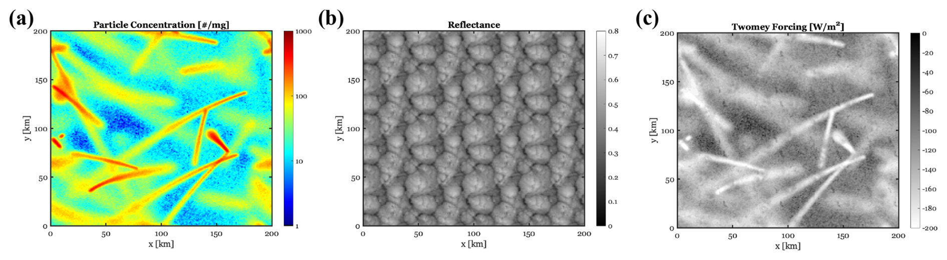
Figure 2 Example snapshot of the particle model concentration-LES cloud field merging process with (a) being the particle model boundary layer-averaged perturbed aerosol concentration output at a given time, (b) the tiled unperturbed reflectance field (to match the domain size of the particle model) from the LES, and (c) the computed Twomey forcing using Eq. (11), with shortwave reflectance, LES background aerosol, and LPM perturbed aerosol concentrations used as the inputs.

All particle model simulations were performed on a 200×200 km² horizontal domain with doubly periodic boundary conditions. A 200×200 km² domain was used to minimize artificial plume self-interaction under periodic boundary conditions on diurnal timescales and to capture changes in plume geometry, such as elongation and changes in plume-axis orientation, associated with ship motion and time-varying mean winds. The ship plumes are initialized with a Gaussian particle position distribution that has a standard deviation (σ) of 1 km in both the x and y dimensions and no initial velocity perturbations. Ship motions are determined randomly from a sample of 8 possible compass directions (N, NE, E, SE, S, SW, W, NW) with a default ship velocity of 10 m s⁻¹. If a ship leaves the domain, its position and compass direction are randomly regenerated with the number of ships within the domain at any given time remaining fixed.

While the LES calculates wet scavenging within the aerosol microphysics, the impacts of scavenging processes (both wet and dry) are approximated in the particle model using a range of aerosol decay timescales (τ_decay=0.25, 0.5, 1, 2 d), with the probability of a particle being removed (P_removal) from the population given by the exponential decay function

$$\begin{array}{}\text{(8)}& P_{\mathrm{removal}}=\exp \left(-{\displaystyle \frac{{\mathrm{age}}^{*}}{{\mathit{\tau }}_{\mathrm{decay}}}}\right),\end{array}$$

where age^* is the particle age calculated as the time elapsed since injection. Particles are removed randomly from each batch of released particles if P_removalS_batch≥1. This age-dependent removal represents the accumulated probability of removal processes over the history of a particle batch, rather than implying that particle age itself is the physical cause of removal.

The Day 1 and Day 2 portions of each trajectory are run separately and represent distinct meteorological regimes with differing boundary layer depths, precipitation, mean winds, background aerosol, and turbulence (see Sect. 3.1). To approximate equilibrium conditions representative of multi-day, repeated injections as expected in an MCB scenario, we repeat the 12 h daytime aerosol injection until the domain-mean peak aerosol concentration changes by less than 2 % between consecutive days. Under this criterion, the number of repeated diurnal cycles necessary for periodic equilibrium for τ_decay=0.25, 0.5, 1, 2 d is 1, 2, 4, and 8 cycles (days), respectively. Interpolated LES fields are smoothed with a 3 h averaging window to avoid sharp discontinuities from morning to night. Unless stated otherwise, aerosol injections begin at sunrise each day and continue for 12 h each day. To derive plume widths and spreading rates from the LPM, a single batch of particles is released and the 2σ width (single σ multiplied by 2) of the x and y particle positions is calculated as done in McMichael et al. (2024), neglecting particle decay/removal.

2.4 LES/LPM merging and Twomey forcing calculation

The Twomey forcing is diagnosed at 20 min intervals (the LES statistics output frequency) by merging the 2D LPM aerosol perturbation fields ($N_{\mathrm{a}}^{\prime }(x_{\mathrm{lpm}},y_{\mathrm{lpm}},t)$; Fig. 2a), defined on the LPM grid (x_lpm, y_lpm), with the radiative fields from each LES case, defined on the LES grid (x_les, y_les). The LES output provides the net shortwave radiative flux at TOA (SW${}_{\mathrm{net}}(x_{\mathrm{les}},y_{\mathrm{les}},t)$) and the total incoming shortwave insolation at TOA (F_inc(t)), from which a scene reflectance (R_scene) can be computed using

$$\begin{array}{}\text{(9)}& R_{\mathrm{scene}}=-{\displaystyle \frac{\left({\mathrm{SW}}_{\mathrm{net}}-F_{\mathrm{inc}}\right)}{F_{\mathrm{inc}}}}.\end{array}$$

R_scene contains the detailed cloud morphology information available from the LES (Fig. 2b).

The doubly periodic LES grid is tiled and clipped to match the size of the 200×200 km² LPM domain. The R_scene field is then coarse-grained to map from 100 m grid spacing in the LES to the 1 km bin size in the LPM by averaging the 10×10 chunk of grid boxes from the LES. We denote the tiled, clipped, and coarse-grained LES field as $\stackrel{\mathrm{‾}}{R}(x_{\mathrm{lpm}},y_{\mathrm{lpm}},t)$. The R_scene values below 0.07 are set to zero to limit the inclusion of clear-sky/ocean-like reflectances. An example snapshot of the 2D R_scene field is shown in Fig. 2b.

Droplet concentration perturbations can be converted to changes in $\stackrel{\mathrm{‾}}{R}$ using Twomey's albedo susceptibility equation (Twomey, 1977; Wood, 2021):

$$\begin{array}{}\text{(10)}& \mathrm{\Delta }\stackrel{\mathrm{‾}}{R}={\displaystyle \frac{\stackrel{\mathrm{‾}}{R}(\mathrm{1}-\stackrel{\mathrm{‾}}{R})\left(r_{\mathrm{n}}^{\mathrm{1}/\mathrm{3}}-\mathrm{1}\right)}{\mathrm{1}+\stackrel{\mathrm{‾}}{R}\left(r_{\mathrm{n}}^{\mathrm{1}/\mathrm{3}}-\mathrm{1}\right)}},\end{array}$$

where $r_{\mathrm{n}}=\left(\frac{N_{\mathrm{a}}^{\prime }+N_{\mathrm{a},\mathrm{les}}}{N_{\mathrm{a},\mathrm{les}}}\right)$, with N_a,les being the time-dependent, boundary layer-averaged background accumulation mode aerosol concentration from the LES. Twomey forcing depends on N_d, but we make the assumption that all aerosol is activated so that N_d=N_a. As mentioned in Wood (2021), the primary sensitivity in Eq. (10) is the perturbation ratio term (r_n) and not changes in $\stackrel{\mathrm{‾}}{R}$. The reflectance changes ($\mathrm{\Delta }\stackrel{\mathrm{‾}}{R}(x_{\mathrm{lpm}},y_{\mathrm{lpm}},t)$) are converted to the indirect shortwave radiative forcing (Twomey forcing) with

$$\begin{array}{}\text{(11)}& \mathrm{\Delta }{F}_{\mathrm{grid}}=-F_{\mathrm{inc}}\mathrm{\Delta }\stackrel{\mathrm{‾}}{R},\end{array}$$

and an example snapshot of ΔF_grid is shown in Fig. 2c. The particle model ΔF_grid is converted to global mean Twomey forcing (ΔF) by averaging ΔF_grid over all LPM grid boxes and times during the final 24 h period of the equilibrium LPM simulations and multiplying that value by the fraction of global surface area that is assumed to be actively sprayed (taken to be 3.147 %) with a given sprayer density. This assumes that the sprayed ocean area is 4000×4000 km² (4.4 % of the ocean area), consistent with recent global modeling studies targeting the most susceptible cloud regions, primarily the northeast and southeast Pacific during the summer months (Chen et al., 2025). The primary ship densities explored in this paper represent low-end (N_sprayers=4000) and mid-range (N_sprayers=16 000) MCB deployments (Wood, 2021), where we expect spreading rate impacts to potentially be most relevant. For N_sprayers=4000 (16 000) , there are 10 (40) sprayers active in the particle model domain during the injection period, corresponding to a ship density of $\mathrm{2.5}\times {\mathrm{10}}^{-\mathrm{4}}$ ships per km² (10⁻³ ships per km²) with a characteristic sprayer spacing of ≈63 km (32 km). For comparison with Wood (2021) and global modeling studies, it is helpful to define the injected salt mass rate (M_s; Tg yr⁻¹), assuming a geometric mean dry diameter (D_s) of 100 nm, a geometric standard deviation (S) of 1.6, the density of sodium chloride (ρ_s=2160 kg m³), and N_inj, the following equation from Wood (2021) can be solved

$$\begin{array}{}\text{(12)}& M_{\mathrm{s}}={\displaystyle \frac{N_{\mathrm{inj}}\mathit{\pi }{\mathit{\rho }}_{\mathrm{s}}{D}_{\mathrm{s}}^{\mathrm{3}}}{\mathrm{6}}}\exp \left(\mathrm{4.5}\ln (S{)}^{\mathrm{2}}\right),\end{array}$$

with M_s≈2 Tg yr⁻¹ for N_sprayers=4000 and ≈8 Tg yr⁻¹ for N_sprayers=16 000.

There are two critical assumptions underlying the offline coupling of the LPM aerosol field with LES reflectances. First, we assume that cloud adjustments are negligible, meaning that the primary control on the radiative flux is the Twomey forcing and not LWP and/or cloud fraction changes. Since the aerosol concentrations from the LPM are not fully coupled to the LES, processes like precipitation suppression (Albrecht, 1989), entrainment enhancement related to smaller droplets and shifts in the radiative cooling profile (Ackerman et al., 2004; Igel, 2024), and potential cloud morphology changes associated with ship track/aerosol plume circulations (Wang et al., 2011; Chun et al., 2023; Prabhakaran et al., 2024; McMichael et al., 2024, 2025) are not captured. As outlined in the introduction, there is considerable uncertainty regarding cloud adjustments in high aerosol/MCB environments, but a growing body of observational studies suggests that radiative impacts of cloud adjustments may be minor compared to the Twomey forcing on both regional (Tippett et al., 2024; Diamond et al., 2020) and global scales (Christensen et al., 2026). In Wood (2021), the heuristic model used to estimate global Twomey forcing also assumed negligible cloud adjustments and was in broad agreement with existing LES of ship tracks.

Second, we assume that all injected aerosols are activated in cloudy regions (100 % activation fraction). This choice represents an upper-bound estimate of the Twomey forcing to highlight potential dependencies on plume spreading rates. In reality, activation will be sensitive to aerosol size, number, updraft velocity, and supersaturation, all of which vary in both space and time (Wood, 2021). As a result of these assumptions, the forcing should be interpreted as the cloud-state-prescribed sensitivity of reflectance to droplet number, rather than a fully coupled response of the cloud field to the aerosol.

Despite the simplifying assumptions of negligible cloud adjustments and 100 % activation, the LES-LPM merging process represents complex, non-linear interactions by capturing the spatial overlap between aerosol perturbations and cloud reflectance fields. Given the stochastic nature of both the Langevin particle model and ship motion, some degree of run-to-run variability is expected; however, even at low sprayer densities (N_sprayers=2000) the run-to-run variability in Twomey forcing is less than 3.5 %, suggesting LPM ensembles of each LES case are not necessary. The Twomey forcing is marginally sensitive to S_p, with S_p=1000 producing 0.7 %–1.8 % less forcing than simulations using S_p=2000.

3 Results and discussion

3.1 Macrophysical, microphysical, and turbulence properties of cloudy LES cases

The cloudy LES cases evolve consistently with theoretical, modeling, and observational understanding of climatological changes along equatorward-moving trajectories, which typically involve decreasing cloud fraction, LWP, and accumulation mode aerosol (NA_c), along with increasing surface precipitation occurrence, deepening boundary layers, and larger mesoscale cellular structures (Wyant et al., 1997; Sandu et al., 2010; Sandu and Stevens, 2011; Wood, 2012; Eastman and Wood, 2016; de Roode et al., 2016; Yamaguchi et al., 2017; Mohrmann et al., 2019; Bretherton et al., 2019; Erfani et al., 2022) (Fig. 3).

Figure 3 Time series of (a) cloud fraction, (b) liquid water path (LWP), (c) boundary layer-averaged accumulation mode aerosol (NA_c), (d) surface rain rate, (e) inversion height, and (f) mesoscale cell size for the cloudy LES ensemble. The top panels show each individual LES simulation, while the bottom panels show the ensemble median (black line) and IQR (green shaded region). Bold black numbers correspond to Day 1 and Day 2 ensemble averages.

Cloud fraction varies considerably between individual LES cases (captured by $\stackrel{\mathrm{‾}}{R}$), experiencing abrupt changes at times, with collapses near midday and recoveries in the evening, in agreement with satellite observations of NEP clouds (Burleyson and Yuter, 2015) (Fig. 3a). The median cloud fraction on Day 2 of the trajectories is ∼25 % lower than Day 1 during the midday hours (Fig. 3a), representing a gently transitioning environment rather than the full stratocumulus-to-cumulus transition where cloud fractions would be expected to be much lower. The LWP evolution generally mirrors the cloud fraction behavior (Fig. 3b) and agrees well with satellite and aircraft observations, with peak LWP near the morning hours and minimum LWP in the late evening (Wood et al., 2002; Mohrmann et al., 2019). The median boundary layer-averaged NA_c is on the order of 100 # mg⁻¹ on Day 1 as observed during the CSET campaign (Bretherton et al., 2019), which declines by nearly half on Day 2 (Fig. 3c). Surface precipitation is minimal on Day 1, but becomes much more common on Day 2, with several cases with surface rain rates greater than 1 mm d⁻¹ (Fig. 3d). Initial median boundary layer depth is near 1 km, growing to nearly 1.5 km on Day 2, with a corresponding increase in the characteristic mesoscale cell size (Wood and Hartmann, 2006), which is calculated by coarse-graining the horizontal velocity fields and counting the number of consecutive grid boxes of a given sign (Fig. 3e and d). Mesoscale cell sizes are generally smaller than reported sizes in Wood and Hartmann (2006), which may be related to domain-size limitations in the LES. Figure S1 in the Supplement provides an example of the counting method used to calculate mesoscale cell size.

The particle model forcing from the LES also has distinct differences in boundary layer-averaged mean winds, velocity variances, and relaxation timescales (T_L) from Day 1 to Day 2 (Fig. 4). Mean winds are consistent with regional climatological winds associated with persistent subtropical high pressure (Mohrmann et al., 2019), as initially stronger north/northeasterly winds slacken and become more easterly on Day 2 (Fig. 4a and b).

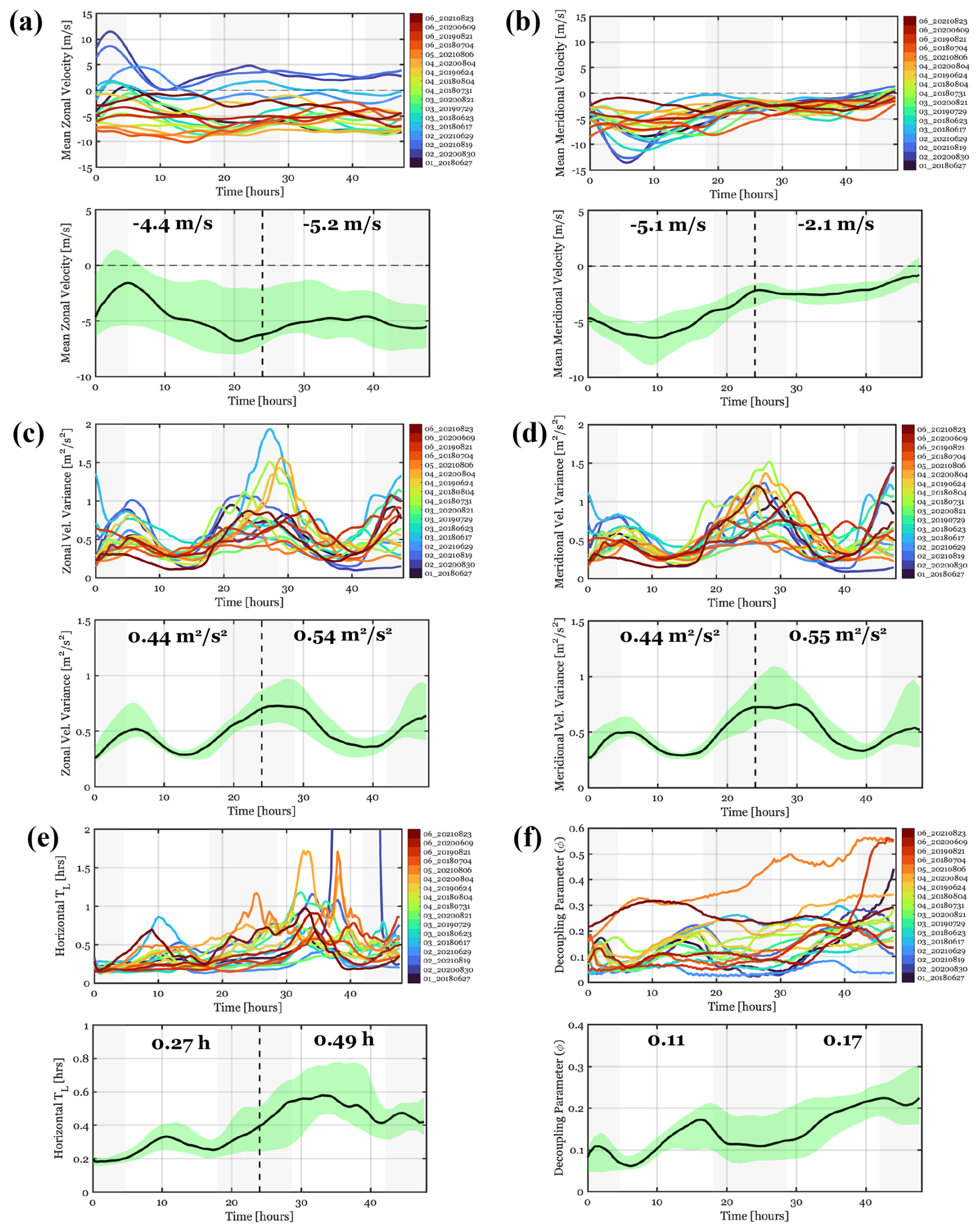
Figure 4 Time series of (a) mean zonal velocity, (b) mean meridional velocity, (c) zonal variance, (d) meridional variance, (e) horizontal relaxation timescale, and (f) the decoupling parameter (ϕ) for the cloudy ensemble.

Horizontal velocity variances show a clear diurnal cycle with maximum variances in the early morning hours and minimum variances in the late evening hours (Fig. 4c and d) related to daytime solar absorption that suppresses TKE production and reduces entrainment (Caldwell et al., 2005; McMichael et al., 2019). The IQR of horizontal variances narrows considerably during the evening hours on both Day 1 and Day 2, despite large differences in boundary-layer depth, precipitation, LWP, and cloud fraction among cases. This behavior supports the idea that the cloud-radiation-turbulence-entrainment feedback acts to limit intercase spread (Zhu et al., 2005). Larger LWP and deeper boundary layer cases have greater cloud-top negative buoyancy fluxes which drive stronger entrainment and may be more prone to drizzle, with both of these mechanisms promoting decoupling and limiting the ability of the cloud-top TKE production to be effectively mixed within the boundary layer. Thinner clouds have smaller cloud-top buoyancy fluxes, but can more easily mix TKE throughout the boundary layer depth. As a result, the IQR range of daytime LWP from 25–55 g m⁻² corresponds to a narrow range of boundary layer-mean horizontal variances (McMichael et al., 2019), with higher case-to-case variability in the early morning hours. On average, Day 2 has ∼25 % larger velocity variances than Day 1; however, Day 2 variances near sunrise are ∼50 % larger than Day 1.

The relaxation timescale (T_L) is almost a factor of 2 larger on Day 2 (Fig. 4e), suggesting that all else equal, particles would revert back to the mean more slowly, resulting in faster Day 2 spreading. It is useful to define a decoupling parameter (ϕ) to quantify the extent of decoupling (Park et al., 2004; Wood and Bretherton, 2004),

$$\begin{array}{}\text{(13)}& \mathit{\varphi }={\displaystyle \frac{q_{\mathrm{t},\mathrm{cl}}-q_{\mathrm{t},\mathrm{sc}}}{q_{\mathrm{t},\mathrm{ft}}-q_{\mathrm{t},\mathrm{sc}}}},\end{array}$$

where q_t,cl is the total water mixing ratio in the cloud layer, subcloud layer (q_t,sc), and free troposphere (q_t,ft). As the boundary layer deepens on Day 2, ϕ increases by approximately 50 % across the ensemble (Fig. 4f), consistent with observational estimates of decoupling in the northeast Pacific (Wood and Bretherton, 2004). The T_L evolution is strongly correlated with the mesoscale cell size (R²=0.59) and the degree of decoupling (ϕ) (R²=0.32), since the dissipation rate is sensitive to both flow geometry and stratification (Fig. S2).

In our merged LES-LPM modeling framework, cloud fraction, LWP, NA_c, precipitation, boundary layer depth, mean winds, vertical velocity variances, and relaxation timescales may all influence Twomey forcing in nonlinear ways. As shown in Fig. 3, the Day 1 and Day 2 states represent distinct meteorological, aerosol, and turbulence regimes along the trajectories and provide an opportunity to probe Twomey forcing sensitivity in each environment.

3.2 LPM-derived plume spreading rates

Horizontal aerosol plume widths vary substantially with the turbulence forcing used in the LPM, with the slowest- and fastest-spreading cases in the cloudy LES library differing by as much as 80 km after 48 h (Fig. 5a). Across the ensemble, plume width is well approximated by a linear growth rate of 1.5 km h⁻¹ (Fig. 5b), consistent with existing LES estimates of lateral plume spreading (McMichael et al., 2024, 2025) and with the observational estimate of 1.85 km h⁻¹ reported by Durkee et al. (2000). Although the ensemble-median plume width is well described by a linear spreading rate, the instantaneous spreading rate exhibits a pronounced diurnal cycle (Fig. 5c and d) associated with diurnal variations in the horizontal velocity variances and T_L. There are several instances of plume spreading rates in excess of 3 km h⁻¹, predominantly occurring in the early morning hours (Fig. 5c). On average, Day 2 median spreading rates are 0.3 km h⁻¹ faster than Day 1 (∼20 % faster), but median spreading rates a few hours after sunrise vary by more than 1 km h⁻¹ (Fig. 5d).

Figure 5 LPM-derived (a) LES case plume width, (b) LES library median and IQR plume width, (c) LES case plume spreading rate, and (d) LES library median and IQR plume spreading rate. Red dashed line on panel (b) corresponds to a 1.5 km h⁻¹ growth rate. Particle batch was released a time = 0 h and tracked for 48 h.

In the Twomey forcing sensitivity analyses that follow, the Day 1 and Day 2 LPM simulations are treated as distinct climatological regimes, with injections initiated at sunrise and active injections for 12 h each day until equilibrium concentrations are reached. To better quantify plume spreading differences between these regimes, spreading rates were calculated from particle batches released at sunrise each day. During most daylight hours, median Day 2 spreading rates exceed those on Day 1 by approximately 1–2 km h⁻¹ (Fig. 6). At night, spreading rates are slightly higher on Day 1 than on Day 2 (Fig. 6c). These results indicate that the two regimes differ not only in their background cloud and boundary layer properties, but also in the rate at which injected aerosol is dispersed, which has the potential to alter aerosol concentration probability distributions and the associated Twomey forcing. Day 2 has a higher incidence of surface precipitation, therefore, C₀ values are adjusted accordingly. However, early morning spreading rates are controlled primarily by changes in variances and not C₀ (Fig. S3). After 5 or so hours after the start of the injection, precipitation-related changes in C₀ result in a 0.5–1 km h⁻¹ acceleration of the plume spreading rate during the midday period (Fig. S3).

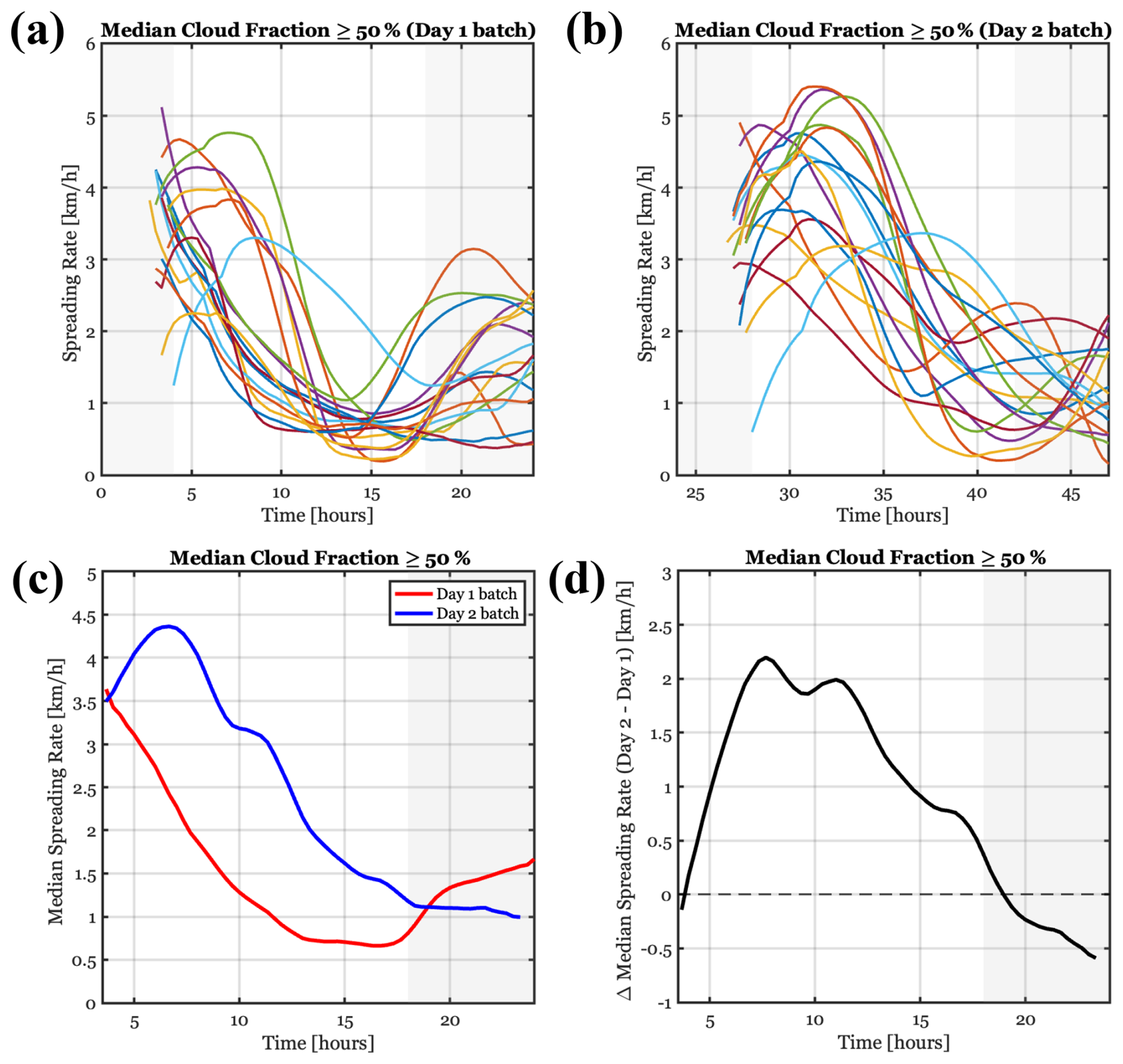
Figure 6 LPM-derived spreading rates for particle batches released at sunrise on Day 1 (a) and Day 2 (b), (c) median spreading rates for Day 1 and Day 2 particle batches, and (d) the difference in median spreading rate (Day 2 − Day 1).

3.3 Twomey forcing sensitivity to northeast Pacific climatology

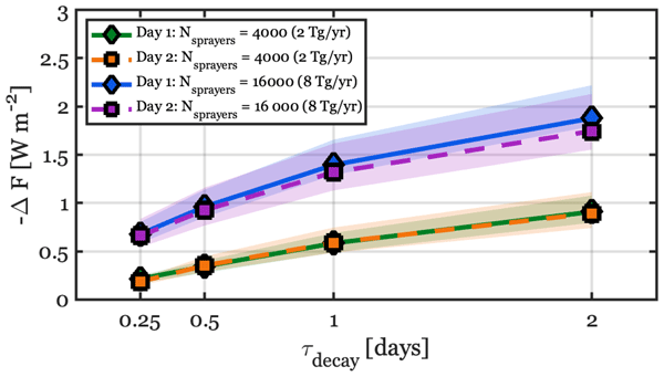
Global mean forcing estimates (ΔF) from the merged LPM-LES library are of the same order of magnitude as implied by the heuristic framework of Wood (2021) for the same total injected mass, although larger. For example, at 8 Tg yr⁻¹, τ_decay=2 d, and N_sprayers=16 000, our model suggests ΔF=1.8 W m⁻² (Fig. 7), compared with about 1 W m⁻² in Wood (2021). The difference likely arises because our sprayers are limited to 4.4 % of the ocean surface rather than distributed across the entire eligible ocean area (54 %) and the injections are occurring preferentially in cloudy regions. As an additional point of comparison, Chen et al. (2025) found that by selectively spraying eastern Pacific cloudy regions (∼5 % of the ocean surface), nearly 1 °C of cooling was achieved. Assuming the mid-range injection scenario and τ_decay=2 d, $\mathrm{\Delta }F=-\mathrm{1.8}$ W m⁻² would impute a temperature sensitivity of 0.56 °C per W m⁻², which is broadly consistent with GCM estimates of temperature sensitivity for spatially inhomogeneous forcing (Hirasawa et al., 2026). While the aim of this study is not to accurately determine ΔF, it is encouraging that the ΔF magnitudes are within a plausible range.

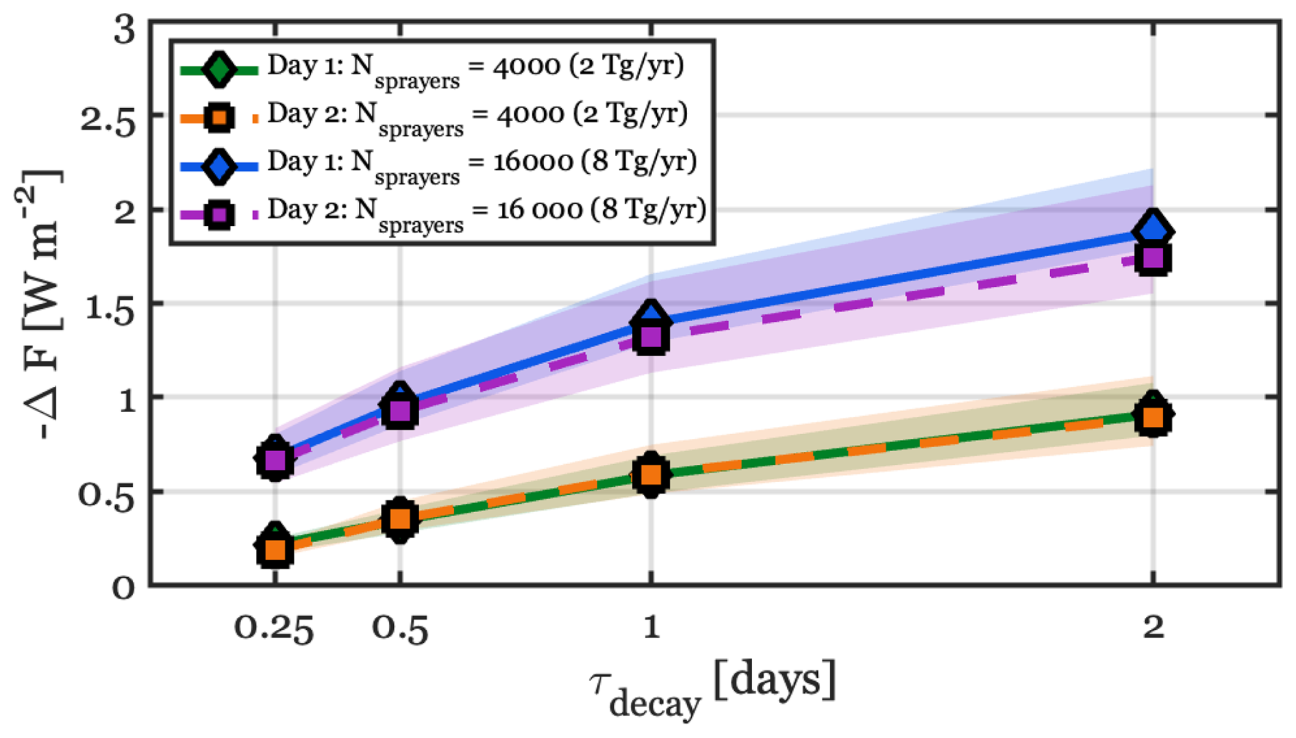
Figure 7 Global mean Twomey forcing (ΔF) as a function of particle lifetime (τ_decay). Green and orange markers correspond to the low-end MCB scenario with N_sprayers=4000 and blue and purple markers correspond to the mid-range MCB scenario with N_sprayers=16 000. Each marker represents the ensemble average global mean Twomey forcing and the shading represents the interquartile range (IQR) of the ensemble.

As shown in Fig. 7, and consistent with Wood (2021), Twomey forcing increases in strength with longer τ_decay, with the largest fractional increases in −ΔF associated with the shorter aerosol lifetimes. Quadrupling N_sprayers only increases −ΔF by a factor of 2.1 at τ_decay=2 d (Fig. 7), indicating a saturation in forcing efficiency as sprayer density increases. Day 1 and Day 2 ΔF differ by less than 8 % for all values of τ_decay and at both the low- and mid-range ship densities (N_sprayers=4000, 16 000) (Fig. 7). This weak regime sensitivity suggests that for a fixed τ_decay and negligible cloud adjustments, the deeper boundary layer and slightly more broken cloud conditions on Day 2 are approximately as susceptible to aerosol perturbations as the more overcast, shallower boundary layers on Day 1. The particle lifetime (set by τ_decay) is the leading-order control on global mean Twomey forcing given a fixed sprayer density.

It is not immediately clear which of the meteorological, aerosol, and turbulence variables are most responsible for the weak regime sensitivity. To assess their relative roles, we perform a sensitivity analysis in which Day 2 values of boundary-layer depth, cloud fraction/morphology, particle model turbulence forcing, mean winds, and background aerosol concentration are substituted individually into the corresponding Day 1 simulations for each case, while all other variables retain their Day 1 evolution. We then quantify the resulting change in ΔF relative to the corresponding Day 1 control simulation.

Deeper boundary layers (which dilute the aerosol perturbation over a greater depth) and lower Day 2 cloud fractions both act to reduce Twomey forcing by 10 %–20 % relative to the Control, while the influence of mean winds is negligible (Fig. 8a). The predominant factor counteracting these reductions is the cleaner background aerosol environment on Day 2, resulting in a nearly 50 % increase in Day 1 Twomey forcing (Fig. 8a). Crucially, and of great relevance to this work, the Twomey forcing is insensitive to changes in the spreading rate between regimes (Fig. 8a). However, while the domain-averaged forcing remains stable when particle forcing is swapped, the underlying aerosol concentration distributions are impacted, with faster spreading rates resulting in reduced frequency of the smallest concentrations and more frequent extreme concentrations (Fig. 8b).

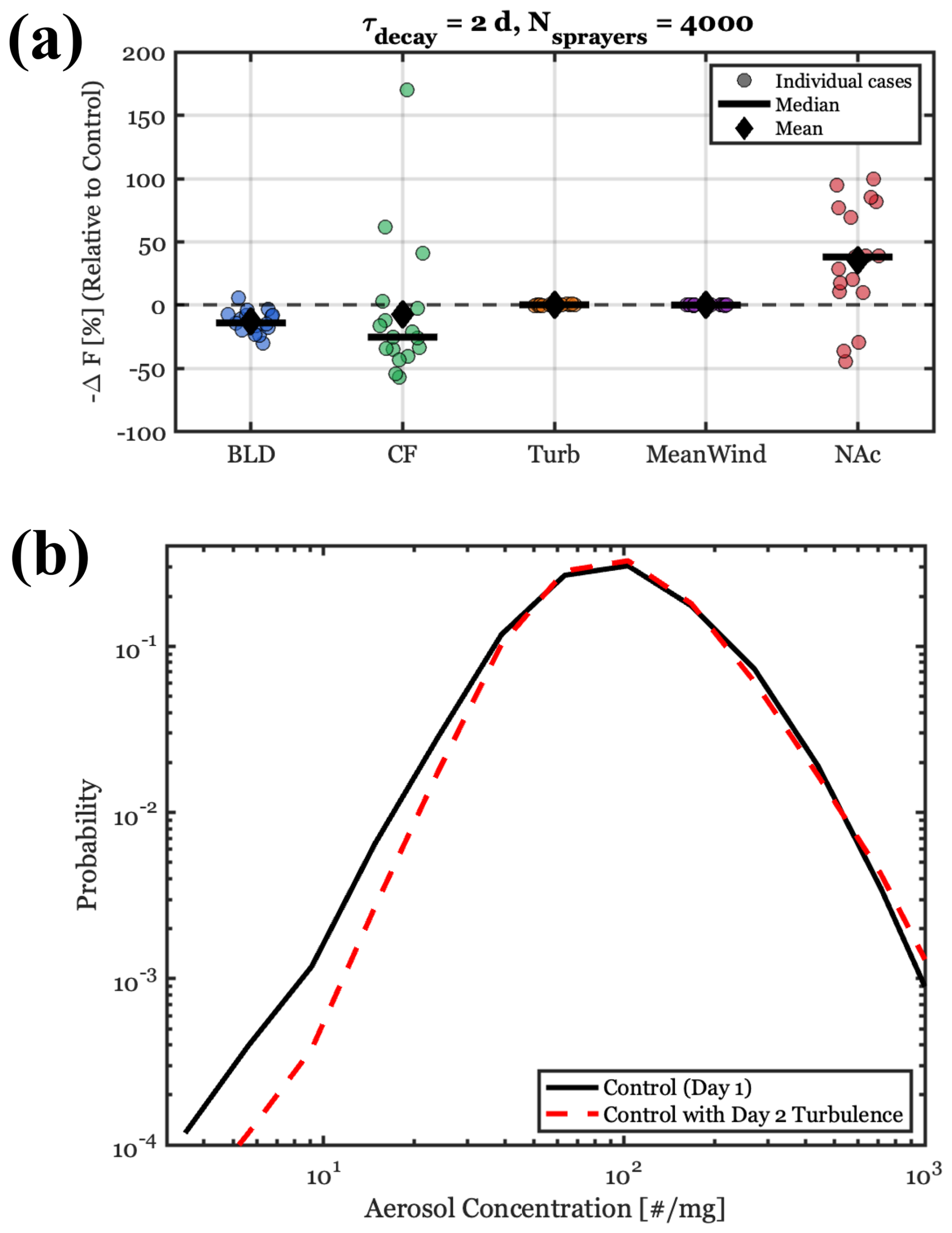
Figure 8 (a) Twomey forcing sensitivity analysis for τ_decay=2 d and N_sprayers=4000, where BLD is the boundary layer depth, CF is the cloud fraction/cloud reflectance, Turb is the particle model turbulence forcing that controls the spreading rate, which includes the C₀ changes related to precipitation, MeanWind is the mean wind, and NA_c is the background aerosol concentration. Positive percentages indicate that Day 2 values of a given variable act to increase Twomey forcing relative to Day 1 values. The circles represent each LPM simulation, the diamond is the ensemble mean, and the line is the ensemble median. (b) Average aerosol concentration probability distributions across all cases at local noon for the Control (Day 1 regime) and the Control run using Day 2 turbulence forcing in the particle model.

3.4 Twomey forcing sensitivity to sprayer motion, injection duration, and injection timing

To our knowledge, the sensitivity of MCB forcing to sprayer velocity has received little direct attention in the literature. Sprayer velocity is potentially important as it constrains platform design and dictates total energy demand, which could increase substantially if high operating velocities are required. Given a theoretical understanding of the diminishing returns of Twomey forcing at high concentrations, it seems logical to assume that higher ship velocities would spread aerosol over larger regions, thus increasing Twomey forcing efficiency. However, the LPM results indicate that the Twomey forcing is largely insensitive to the ship velocity, with velocities ranging from 0 to 10 m s⁻¹ changing ΔF minimally (Fig. 9a). While the area-averaged forcing of ΔF remains nearly constant, the spatial distribution of the perturbed aerosol concentration does change, most notably at ship velocities of 10 m s⁻¹, with reduced occurrence of low concentrations and more frequent concentrations in the 20–80 # mg⁻¹ range (Fig. 9b). By running the LPM simulations with no mean wind ($\stackrel{\mathrm{‾}}{U_t}=\mathrm{0}$ in Eq. 3), the sensitivity to ship velocity emerges with ship velocities below 5 m s⁻¹ resulting in dramatically reduced cooling efficiency (Fig. 9a). In the no mean wind scenario experiments, underlying probability distributions of aerosol concentrations begin to shift considerably, with the most susceptible Twomey forcing range experiencing reduced probabilities and a marked increase in concentrations above 200 # mg⁻¹ (Fig. 9b). This finding suggests that in environments like the northeast Pacific, the energy and mechanical requirements of MCB could be meaningfully reduced by utilizing stationary or slow-moving platforms without compromising radiative efficacy. Of course, it remains possible that this result could be impacted by processes that control the vertical dispersion of aerosols in different environments (i.e., evaporation, local buoyancy perturbations) (Dhandapani et al., 2025). Simulations using uniformly-spaced sprayers moving in parallel, rather than randomly moving sprayers, indicate that Twomey forcing is also insensitive to ship organization (not shown).

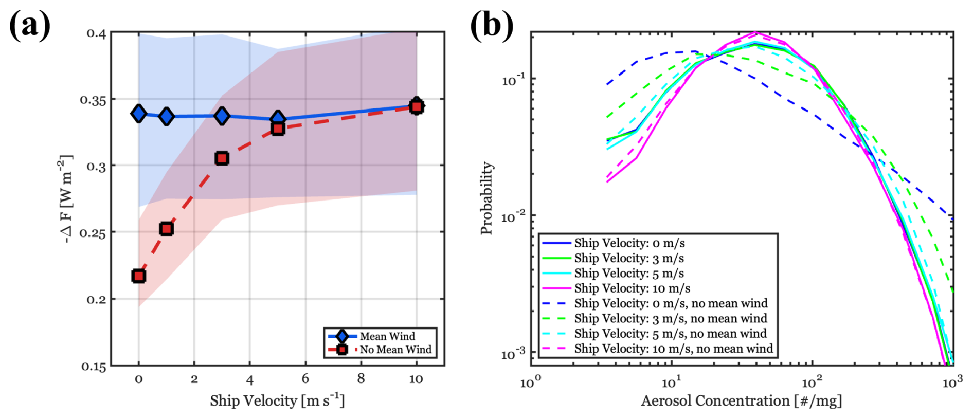
Figure 9 (a) Markers indicate the ensemble-averaged global mean Twomey forcing sensitivity to ship velocity for time-varying mean winds (Blue) and no mean wind (Red). Shading corresponds to the IQR of the ensemble. (b) Ensemble mean aerosol concentration probability distributions as a function of ship velocity and mean wind/no mean wind. Sensitivity tests using τ_decay=0.5 d and N_sprayers=4000.

The global mean Twomey forcing scales roughly linearly with increasing injection duration, with the slope of the increase depending on the assumed value of τ_decay (Fig. 10a). Longer τ_decay is associated with higher sensitivity to the injection duration, with τ_decay=2 d resulting in 0.06 W m⁻² h⁻¹ of injection and τ_decay=1 d resulting in 0.04 W m⁻² h⁻¹ of injection (Fig. 10a). Given 50 % increases in Twomey forcing from 6 to 12 h injection duration, it is likely worthwhile to continue injecting well after the “peak” susceptibility window in the morning hours (Jenkins et al., 2013). The sensitivity to injection timing is generally consistent with the modeling studies of Jenkins et al. (2013), with 10 %–25 % enhancement in Twomey forcing achieved by injecting in the early mornings hours, versus a few hours after sunrise (Fig. 10b).

Figure 10 Ensemble-averaged global mean Twomey forcing as a function of (a) the daily injection duration for τ_decay of 1 and 2 d and (b) the injection timing relative to sunrise, for a 12 h daily injection. Shading corresponds to the IQR of the ensemble. Sensitivity tests use N_sprayers=4000.

3.5 Twomey forcing as a function of particle age and concentration bin

The particle model allows for the explicit tracking of particle age and the associated Twomey forcing from each particle age group. With τ_decay=2 d, periodic equilibrium is reached after 8 d in the particle model, which means the maximum particle age is 8 d, despite the LES only having a run time of 2 d. Although not a strong function of N_sprayers or case-to-case variability, the percentage of Twomey forcing from a given particle age group is strongly dependent on τ_decay, as expected, with 3+ day old particles contributing to 2 % of the forcing when τ_decay=1 d and 41 % of the forcing when τ_decay=4 d (Fig. 11a). Aerosols less than 1 d old are responsible for 25 %–65 % of the Twomey forcing, while aerosols 1–3 d old contribute close to 35 % across the τ_decay range (Fig. 11a).

Figure 11 (a) The percent of Twomey forcing as a function of particle age for N_sprayers=800 and τ_decay of 1, 2, and 4 d. (b) The percent of Twomey forcing from each particle concentration bin for τ_decay=2 d. Bold lines represent the LES ensemble mean percentage of total Twomey forcing (left y axis) and the dashed lines correspond to the cumulative percentage of Twomey forcing going from left to right in the bin space (right y axis). Different colors are for different values of N_sprayers.

In addition to particle age, we quantified the contribution of each particle concentration bin to the Twomey forcing. For each bin, Twomey forcing was summed over all particle model grid cells falling within that concentration range. The contribution from each bin was then expressed as a percentage of the domain-total Twomey forcing (Fig. 11b). Our results reveal that for N_sprayers≤1600, only 10 %–15 % of the total Twomey forcing originates from concentration bins > 120 # mg⁻¹ assuming τ_decay=2 d (Fig. 11b), emphasizing the difficulty of detecting the Twomey-forcing relevant aerosol perturbations (Yuan et al., 2025), even in regions of relatively dense ship traffic. In the low-end MCB scenario (N_sprayers=4000), only 20 % of the forcing originates from bins below 120 # mg⁻¹ (Fig. 11b), making such a perturbation easily detectable.

3.6 Theoretical importance of spreading rate for GCMs

We explore the maximum theoretical importance of spreading rate and quantify potential errors associated with assumptions made in GCMs (i.e., infinite spreading rate and uniform aerosol concentrations) using a changing particle model domain size with a single, fixed point source at the center of the domain. With doubly periodic boundary conditions, the changing domain size is a proxy for ship density. Cloud fraction is assumed to be unity, background aerosol is fixed at 20 # mg⁻¹, and boundary layer depth is constant at 1 km, to maximize the potential importance of spreading rate. First, we examine the fastest (FAST) and slowest (SLOW) spreading cases in the LES library, which have daily average spreading rates of 3.18 and 0.2 km h⁻¹, respectively. The difference between these two cases represents the upper bound on expected spreading-related Twomey forcing errors for naturally varying turbulence conditions, and the Twomey forcing magnitude and percentage differences are shown in Fig. 12a and b. For N_sprayers<5000 or a ship density < $\mathrm{3.125}\times {\mathrm{10}}^{-\mathrm{4}}$ ships per km², spreading rate-related Twomey forcing errors could potentially be in the 5 %–30 % range (Fig. 12b). Beyond N_sprayers=20 000 ($>\mathrm{1.25}\times {\mathrm{10}}^{-\mathrm{3}}$ ships per km²), errors related to spreading rates are likely to be small.

Figure 12 The theoretical maximum importance of spreading rate explored using a changing domain size with a single, fixed point source at the center of the domain. Cloud fraction is assumed to be unity, background aerosol is fixed at 20 # mg⁻¹, and boundary layer depth is constant at 1 km, to maximize the potential importance of spreading rate. (a) FAST-SLOW difference in global mean Twomey forcing, (b) FAST-SLOW percentage increase in global mean Twomey forcing, (c) INF-SLOW difference in global mean Twomey forcing, and (d) INF-SLOW percentage increase in global mean Twomey forcing. The different colored lines correspond to the different aerosol lifetime assumptions (τ_decay).

To estimate an upper bound on potential Twomey forcing errors in GCMs, we compare the SLOW case to the assumption made in current GCM simulations of MCB, which is that the aerosol is instantaneously spread evenly throughout the grid box. The working assumption in current GCM implementations is that the spreading rate is infinitely fast (INF), with Fig. 12c and d showing the Twomey forcing magnitude and percentage differences between the INF and SLOW cases. Errors become much more substantial when making the INF assumption, with ship densities below $\mathrm{2.5}\times {\mathrm{10}}^{-\mathrm{4}}$ ships per km² resulting in 10 %–200 % errors in global mean Twomey forcing, depending on τ_decay (Fig. 12d). Even at sprayer densities representative of high-end MCB scenarios, spreading-related Twomey forcing errors could exceed 10 % in environments where τ_decay is less than 1 d (Fig. 12d).

Additional idealized experiments indicate that concentration variability driven by random overlaps of ship tracks does not strongly impact the spreading rate and Twomey forcing relationship (Fig. S4). Using the median library spreading rate, instead of the extreme SLOW case, the expected spreading-related GCM errors for a mid-range MCB scenario (N_sprayer>10 000) would generally be 10 % or less (Fig. S5). In the context of a mid- to high-end MCB scenario, Twomey forcing is unlikely to be impacted substantially by differences in naturally occurring horizontal spreading rates, but the instantaneous spreading rate assumption may still lead to overestimates of cooling in GCMs. These errors, especially in short aerosol lifetime environments, can be reduced by assuming a fixed, finite spreading rate (e.g., ∼1.5 km h⁻¹).

3.7 Statistical predictions of spreading rate from LES properties

Assuming a finite spreading rate in GCMs could ameliorate some of the spreading-related radiative forcing errors, but in some global injection scenarios sprayer density might be on the lower end of Fig. 12, necessitating a more sophisticated approach to estimating the spreading rate within a GCM. One potential promising predictor of the particle model-derived spreading rate is the boundary layer-averaged horizontal TKE (TKE_hor) multiplied by T_L, which has diffusivity units (m² s⁻¹) and explains nearly 50 % of the variance in spreading rate (Fig. 13). When all times along the trajectories are included there is a clear time dependence of the spreading rate, with earlier times corresponding to faster spreading rates (Fig. 13a). Bearing in mind this time-dependence, the statistical spreading rate relationships may need to vary as a function of time since injection. When the first 10 h of spreading are neglected, the TKE_hor×T_L quantity explains ∼70 % of the variance. In future work, relationships such as these may be implemented within the GCM as an effective plume spreading parameterization. In models that employ CLUBB, such as E3SM (Zhang et al., 2024), T_L and TKE_hor are readily available quantities, but their agreement with LES requires further investigation.

Figure 13 The statistical relationship between particle model-derived spreading rate and TKE_hor×T_L for (a) all times and (b) all times excluding the first 10 h after injection. Colors change as a function of time since injection. Black lines indicate the power-law regression, with the equation and R² values provided in the upper right hand portion of the panels. All times from all cloudy LES ensemble members are shown.

4 Conclusions

In this study, we employ a combination of 2 d, realistically time-varying Lagrangian large-eddy simulations (LES) and Langevin particle modeling (LPM) to investigate the importance of horizontal spreading rate, meteorological, and aerosol variability on Twomey forcing. The analysis focuses on the cloudy LES cases (17 cases with median cloud fraction > 50 %) in the 54-member LES library, as these cases show the strongest agreement with satellite observations and represent prime candidate environments for Marine Cloud Brightening (MCB) deployments. The LPM has previously been shown to reproduce horizontal spreading rates in LESs of single ship tracks in various turbulence and background aerosol environments when forced by boundary layer-averaged turbulence and dissipation rates (McMichael et al., 2024). Explicitly modeling many different sprayer and injection configurations for the LES library is computationally cost prohibitive; however, by leveraging the LPM framework, we can estimate the spatio-temporal evolution of injected aerosol by forcing the LPM with the background meteorology and turbulence data from the LES library.

The Twomey forcing calculation involves merging the 2D LPM aerosol fields with the 2D reflectance fields from the LES. This merging process allows for complicated interactions between aerosol distributions and the cloud morphologies modeled in the LES library; although, the direct mapping of the aerosol concentrations onto the LES cloud fields makes the assumptions that the aerosol is well-mixed in the vertical, 100 % of the aerosol is activated, and cloud adjustments are relatively small compared to the Twomey forcing. A decoupling parameter analysis indicates that many of the cases remain weakly decoupled with minor moisture stratification. Assuming 100 % aerosol activation simplifies the analysis and provides an upper bound on potential spreading rate-driven Twomey forcing differences. If cloud adjustments were taken into account, it is possible that Twomey forcing could be augmented or weakened in certain environments and cloud morphology could change in complex ways (e.g., cloud clearing near ship-track mesoscale circulation boundaries in precipitating environments), depending on background meteorological and aerosol conditions. This work represents a natural extension of the Wood (2021) heuristic framework, where environmentally dependent spreading rates and their interactions with changing cloud morphologies are now estimated.

In the cloudy LES case library, meteorological, aerosol, and turbulence properties responsible for plume spreading differ appreciably between the Day 1 and Day 2 regimes, with Day 2 being characterized by deeper boundary layers, stronger turbulence, longer relaxation timescales, cleaner background aerosol conditions, and lower cloud fraction, all of which are consistent with our understanding of the equatorward evolution of low clouds. Despite these distinct meteorological, aerosol, and turbulence differences, there is weak regime sensitivity to Twomey forcing between Day 1 and Day 2, regardless of the assumed aerosol lifetime (τ_decay) or ship density implied by N_sprayers. A sensitivity analysis shows that the weak regime sensitivity arises because of cleaner Day 2 background aerosol conditions that offset Twomey forcing reductions from reduced cloud cover and deeper boundary layers. The consequence of this is that given a fixed τ_decay and assuming negligible cloud adjustments, the Day 1 and Day 2 regimes are nearly equally susceptible to MCB. Previous LES of ship tracks suggest that the cleaner, precipitating boundary layers may be more prone to positive cloud adjustments that would enhance Twomey forcing, which may mean that the Day 2 regime would ultimately be more efficient (Chun et al., 2023; Prabhakaran et al., 2024); however, the leading-order control on Twomey forcing and the MCB efficiency of each regime is the aerosol lifetime assumption τ_decay, which emphasizes the need for a greater understanding of injected aerosol lifetime-modulating processes such as collision-coalescence, interstitial scavenging, sedimentation, turbulent impaction, coagulation, and entrainment sources/sinks (Wood, 2021).

Day 1 and Day 2 spreading rate regimes differ by over 2 km h⁻¹ at times, with Day 2 relaxation timescales (T_L) that are nearly a factor of 2 larger than those on Day 1. These longer relaxation timescales are associated with dissipation rate decreases related to larger mesoscale cells, more decoupled boundary layers, and modest increases in velocity variances. To isolate the effect of turbulence-driven spreading differences on Twomey forcing, we repeated the Day 1 LPM simulations using the Day 2 turbulence characteristics while maintaining the Day 1 cloud morphology, boundary-layer depth, mean wind, and background aerosol concentration conditions. Despite the substantially faster spreading associated with the Day 2 turbulence, the resulting Twomey forcing changes are smaller than 1 %. Therefore, in these simulations, the differences in turbulence-driven horizontal plume spreading alone do not produce appreciable changes in Twomey forcing, even though the underlying aerosol concentration distributions are impacted by the spreading rate differences.

The spreading rates exhibit a pronounced diurnal cycle, with the strongest spreading rates near sunrise (3+ km h⁻¹) and a dramatic decrease in the spreading rate occurring in the late evening associated with the diurnal cycle of turbulence (∼1 km h⁻¹). The instantaneous spreading rates experience a wide degree of variability, but the ensemble plume width is well-approximated by a linear growth rate of 1.5 km h⁻¹, which is reasonably close to the Durkee et al. (2000) estimate of 1.85 km h⁻¹ used in Wood (2021).

Additional LPM sensitivity tests suggest that Twomey forcing is largely unaffected by changing sprayer velocity (in the 0–10 m s⁻¹ range) and ship motion (random versus organized) in the northeast Pacific mean wind environment, implying that slow-moving or stationary spraying platforms may be viable, assuming efficient vertical transport and subsequent activation. Additionally, there is still forcing upside to injecting for much of the daylight hours (∼12 h versus 6 h), with injections beginning several hours before sunrise being most efficient, in agreement with Jenkins et al. (2013). In an analysis of particle ages and concentration bins, a majority of the Twomey forcing originates from particles > 1 d old and from concentrations below 100 # mg⁻¹.

The relative role of horizontal spreading rate on Twomey forcing across a range of time-varying cloud fields, meteorological, and aerosol conditions is small, but idealized LPM experiments using 100 % cloud fraction and the most extreme spreading rate cases in the LES library indicate that if the range of naturally varying spreading is neglected, Twomey forcing could be overestimated by 5 %–30 % for sprayer densities below $\mathrm{3.125}\times {\mathrm{10}}^{-\mathrm{4}}$ ships per km², with larger errors for shorter aerosol lifetimes. Above a sprayer density of $\mathrm{1.25}\times {\mathrm{10}}^{-\mathrm{3}}$ ships per km², errors from the naturally occurring range of spreading rates tend to zero. However, the spreading rate is much faster in GCMs than the fastest spreading rate in the LES library, as GCMs assume that the plume spreads infinitely fast within a climate model grid box. The infinite spreading rate assumption leads to potential Twomey forcing overestimations of 10 %–200 % at sprayer densities below $\mathrm{2.5}\times {\mathrm{10}}^{-\mathrm{4}}$ ships per km². Even at high sprayer densities representative of a high-end MCB scenario, errors may exceed 10 % for aerosol lifetimes less than 1 d.

In light of the results from our merged LES-LPM framework, there are four primary emergent priorities for the future of plume spreading and Twomey forcing sensitivity research:

• Narrow uncertainties regarding the aerosol lifetime (τ_decay), addressing issues such as potential dry deposition enhancement driven by intense aerosol-induced mesoscale circulations.

• Continue to constrain possible cloud adjustments, accounting for the potential of repeated aerosol injections. Substantial cloud adjustments, with fully coupled aerosols, have the potential to alter the relationship between Twomey forcing and spreading rate found in this paper.

• Develop subgrid plume parameterizations, such as the one discussed in Sect. 3.7, to reduce the risk of overestimating MCB cooling potential in GCMs.

• Further understanding of vertical aerosol spreading rates, realistic activation processes, and aerosol size distribution evolution to more accurately predict N_d in GCMs.

In summary, our results indicate that although horizontal plume spreading rates do not strongly affect global mean Twomey forcing across realistic northeast Pacific MBL regimes when assuming negligible cloud adjustments, the infinite spreading rate assumption inherent in current GCMs may lead to an overestimation of MCB efficiency that should be addressed through physically grounded subgrid plume spreading parameterizations. In addition, aerosol lifetimes differ strongly between precipitating and non-precipitating clouds. Therefore, the co-variability of aerosols and clouds affects the aerosol lifetime, which translates to potentially large changes in Twomey forcing, highlighting the importance of parameterizations of subgrid-scale aerosol and cloud processes in GCMs.