EarthCARE reveals details on the role of rain in closed-to-open cell transitions

The mesoscale organisation of marine stratocumulus clouds into closed and open cells strongly affects cloud albedo and thus their cooling effect on climate, yet the processes governing transitions between these regimes remain incompletely understood. The EarthCARE satellite provides collocated observations of cloud mesoscale structure from the Multi-Spectral Imager (MSI) together with vertically resolved cloud and precipitation measurements from the Atmospheric Lidar (ATLID) and Cloud Profiling Radar (CPR), enabling detailed characterization of stratocumulus cloud microphysics. We apply a convolutional neural network to MSI scenes to identify closed and open cells and relate these classifications to EarthCARE microphysical retrievals from the synergy of ATLID, CPR, and MSI. Open cells exhibit substantially lower droplet number concentrations (N_d), greater variability in liquid water path (LWP) and droplet sizes (r_e), and more frequent and heavier precipitation, although light drizzle is also common in closed cells. To investigate closed-to-open cell transitions, we combine EarthCARE overpasses with GOES/ABI geostationary imagery and ERA5-driven trajectories to track cloud scenes and determine transition timing. This combined approach allows us to reconstruct the temporal evolution of cloud properties around transitions. We find that LWP and rain amounts increase in closed cells up to 25 h before transitions, followed by decreasing N_d and increasing r_e, while cloud vertical structure remains largely unchanged. These findings support a precipitation-linked transition pathway, potentially triggered by enhanced boundary-layer moisture and amplified by aerosol scavenging–rain feedback. This new observational evidence advances our understanding of stratocumulus breakup with implications for the cooling effect of these clouds.

1 Introduction

Marine stratocumulus clouds play a pivotal role in Earth's climate system, reflecting much of the incoming solar radiation back to space. An important aspect of stratocumulus clouds is their mesoscale organization, i.e. cloud pattern organization on horizontal scales of the order of kilometres to 100 km. A prominent manifestation of this mesoscale organization is the occurrence of closed-cell and open-cell stratocumulus (Wood and Hartmann, 2006; Wood et al., 2008; Muhlbauer et al., 2014; Koren et al., 2017; Mohrmann et al., 2021). Closed cells are generally associated with high cloud fraction and high albedo, whereas open cells exhibit broken cloud fields with reduced cloud fraction and lower albedo (Wood and Hartmann, 2006; McCoy et al., 2017; Danker et al., 2022; McCoy et al., 2023). A transition from closed to open cells usually leads to a drop in cloud albedo and consequently the clouds' cooling effect. As a result, uncertainties in the representation of stratocumulus clouds remain a major contributor to the spread in climate sensitivity and cloud feedbacks in climate models (Bony and Dufresne, 2005; Ceppi et al., 2017; IPCC, 2023). Understanding the processes that lead to mesoscale structure changes and the break-up of closed stratocumulus decks is especially pressing in light of new findings that a decrease in cloud fraction of low-level clouds is the main reason for the increasing positive energy imbalance of the Earth (Loeb et al., 2024).

Despite substantial progress, the processes governing transitions between closed and open cells remain incompletely understood. Several mechanisms have been proposed and intensively investigated, including aerosol-cloud-precipitation interactions, cold-pool dynamics, cloud-top entrainment and instability, and the influence of surface forcing and large-scale meteorology (Savic-Jovcic and Stevens, 2008; Wang and Feingold, 2009a, b; Feingold et al., 2010; Yamaguchi and Feingold, 2015; Jensen et al., 2021; Chandrakar et al., 2022; McCoy et al., 2023). In particular, precipitation has long been hypothesized to play a key role in promoting open-cell conditions (Stevens et al., 2005; Wood et al., 2008). Large-Eddy Simulations (LES) show that in simulations with low aerosol concentrations and consequently heavier rain, open cells are the preferred state (Savic-Jovcic and Stevens, 2008; Wang and Feingold, 2009a; Berner et al., 2013; Yamaguchi and Feingold, 2015; Chandrakar et al., 2022; Hoffmann et al., 2023). The proposed physical mechanism is that precipitation weakens the closed-cell circulation by removing cloud water and by evaporative cooling below cloud base, which promotes subcloud stabilization and decoupling. The resulting cold, moist outflows form cold pools whose collisions mechanically trigger updrafts and help organize the cloud field into open cells (Savic-Jovcic and Stevens, 2008; Yamaguchi and Feingold, 2015).

Observational studies from multiple field campaigns and case studies report stronger drizzle and reduced aerosol concentrations in open-cell or pocket-of-open-cells (POC) conditions (Stevens et al., 2005; Sharon et al., 2006; Jensen et al., 2021). Satellite studies have provided evidence that open cells typically consist of fewer, larger cloud droplets and that these cloud structures are associated with stronger winds and lower inversion strength (e.g., Muhlbauer et al., 2014; McCoy et al., 2017; Mohrmann et al., 2021). Recent work has also adopted Lagrangian frameworks to track cloud scenes through time using wind trajectories combined with imagery from polar-orbiting (Eastman et al., 2022) and geostationary satellites (Smalley et al., 2022). These approaches have strengthened evidence that precipitation is closely linked to the closed-to-open transition (Eastman et al., 2022; Smalley et al., 2022).

However, progress has been limited by observational constraints. Passive sensors infer precipitation indirectly and often struggle with light drizzle, large footprints, and limited ability to resolve the vertical distribution of hydrometeors. Additionally, precipitation retrievals are frequently not collocated with the cloud microphysical retrievals used to infer droplet number concentration or effective radius, complicating process interpretation along a Lagrangian track (Smalley et al., 2022). At the same time, other studies have reported that drizzle differences between open and closed cells may be modest in some conditions, suggesting that precipitation-related thermodynamic feedbacks are not the sole factor controlling mesoscale organization (Wood et al., 2011; Terai et al., 2014; Yamaguchi and Feingold, 2015). Further, while aerosol depletion within POCs is frequently observed and may promote precipitation by reducing droplet number concentrations, the causal sequence between precipitation enhancement, aerosol scavenging, and mesoscale breakup remains debated (Wood et al., 2008; Smalley et al., 2022; Eastman et al., 2022; Chandrakar et al., 2022).

The Earth Cloud, Aerosol and Radiation Explorer (EarthCARE), launched in May 2024 (Eisinger et al., 2024), provides a new opportunity to study stratocumulus clouds with unprecedented detail and can address these gaps. Firstly, EarthCARE carries both active (Atmospheric Lidar, ATLID, and Cloud Profiling Radar, CPR) and passive (Multi-Spectral Imager, MSI) sensors on board. This combination provides collocated measurements of mesoscale structure and vertically resolved information of aerosol, cloud and rain properties. Secondly, the EarthCARE CPR overcomes major limitations of earlier missions such as CloudSat by providing enhanced sensitivity, finer vertical and horizontal resolution, and greatly reduced surface-clutter contamination. Using the first year of CPR observations, Xu et al. (2026) show that surface clutter is effectively suppressed above approximately 0.5 km, and that CPR detects substantially more stratocumulus and has an improved identification of precipitation compared to CloudSat's radar instrument in key subtropical regions. Furthermore, as the first spaceborne Doppler radar, EarthCARE's CPR provides vertical velocity estimates tightly linked to raindrop fall speeds. Combining reflectivity and Doppler velocity yields better constraints on raindrop sizes and improves retrievals of rain rate and liquid water content compared to single-frequency radars (Mason et al., 2023). These advances enable more reliable detection and characterization of shallow marine clouds and drizzle close to the ocean surface, a regime that was challenging before. This capability is particularly important for stratocumulus transitions, where drizzle and its subcloud evaporation are thought to be important drivers for cloud breakup (Wood et al., 2008; Yamaguchi and Feingold, 2015; Cadeddu et al., 2020; Smalley et al., 2022; Eastman et al., 2022).

While EarthCARE provides detailed instantaneous information, it is still a polar-orbiting platform and therefore samples any given region infrequently, with a revisit time of about 25 d for the active instruments. Therefore, to study transitions, it is best to combine EarthCARE snapshots with the continuous temporal coverage of geostationary satellites. Geostationary imagery can track mesoscale cloud organization and identify the timing of transitions, while EarthCARE provides a physically rich characterization of the cloud and precipitation column during overpass.

In this study, we exploit this combination of EarthCARE and geostationary satellites to investigate closed and open cell stratocumulus organization and transitions in the subtropics. We address two main research questions:

1. We quantify differences in cloud and precipitation properties between open and closed cells from the perspective of EarthCARE, taking advantage of the satellite's improved capabilities to measure these quantities and a convolutional neural network (CNN) to classify clouds into different mesoscale structures.

2. We examine how these properties evolve in the hours leading up to and following a closed-to-open cell transition. To this end we use a Lagrangian perspective, combining EarthCARE with geostationary measurements of the Geostationary Operational Environmental Satellite (GOES) along wind trajectories. We use this information to assess candidate transition mechanisms, with a focus on the role of precipitation and its associated dynamical feedbacks.

The the paper is structured as follows. Section 2 describes the datasets and methodology, including the EarthCARE cloud and precipitation retrievals, the CNN used for mesoscale structure classification and the tracking framework. Section 3.1 presents the EarthCARE-based contrasts between open and closed cellular regimes. Section 3.2 analyses the time evolution of cloud and rain properties relative to transition time. Section 4 discusses uncertainties, and assesses implications for transition mechanisms and regional generality.

2 Data and Methods

EarthCARE observations used in this study are taken from product baseline BA, covering August 2024 to November 2025. Later observations are available but belong to a subsequent processing baseline and are not included here for consistency. The study domain comprises four well-established subtropical stratocumulus regions: the Southeast Pacific (SEP), Northeast Pacific (NEP), Southeast Atlantic (SEA), and Northeast Atlantic (NEA), each with an extent of 20°×20° longitude and latitude (see Fig. 1). These regions are frequently used for evaluating closed and open cell stratocumulus clouds (Wood and Hartmann, 2006; Wood et al., 2008; Muhlbauer et al., 2014; Mohrmann et al., 2021; Fons et al., 2024).

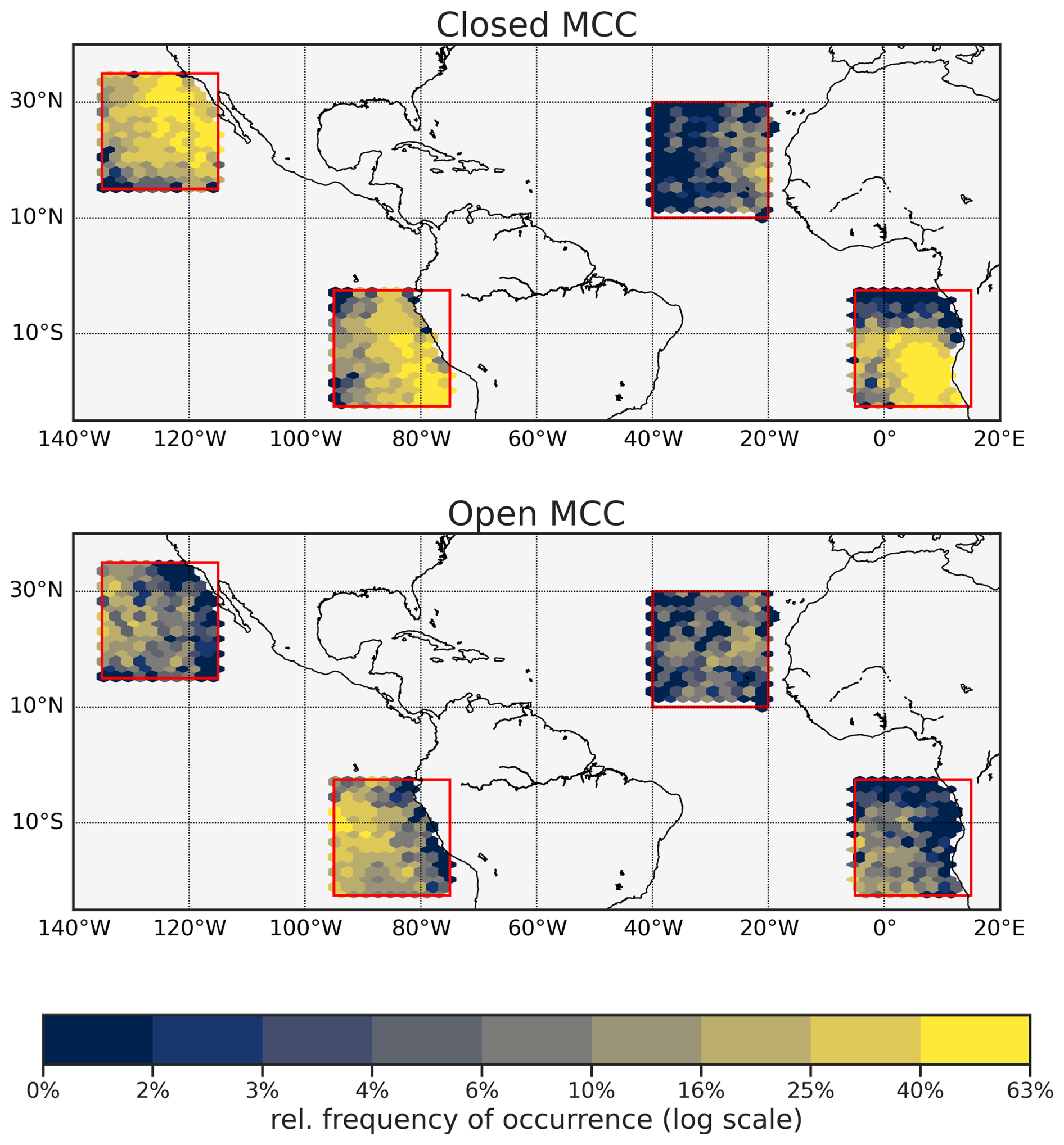
Figure 1 Geographic distribution of closed and open cells in four stratocumulus regions in terms of relative frequency of occurrence. Relative frequency of occurrence is computed as the fraction of occurrences of closed or open cells, as detected by the CNN applied to MSI, to the total number of all mesoscale cloud structure occurrences, expressed as percentage.

We construct a dataset containing EarthCARE observations over the four stratocumulus regions, combining information on cloud and rain properties, with mesoscale cloud-structure characteristics. A CNN is used to classify cloud scenes into mesoscale structure classes, most notably closed and open cells. For the SEP region, we additionally incorporate GOES geostationary data to introduce a temporal dimension, enabling analysis of transitions between closed- and open-cell regimes. The SEP region was chosen out of the four stratocumulus regions for this second part of the study, because it contains the largest number of open cells (see Fig. 1).

In the following subsections, we describe the data sources and processing steps in detail, including the three EarthCARE data products used, the GOES imagery, the wind trajectories, and the CNN-based cloud-scene classification.

2.1 EarthCARE ACM-CAP for detailed cloud and rain observations

The ACM-CAP product provides a synergistic retrieval of clouds, aerosols, and precipitation from the combination of EarthCARE's active and passive instruments, ATLID, CPR and MSI. It uses the CAPTIVATE optimal estimation retrieval framework and delivers a comprehensive set of products including profiles of liquid clouds and rain (Mason et al., 2023). ACM-CAP is unique in that it provides a unified retrieval of all hydrometeors and aerosols. This has the advantage of facilitating retrievals even in complex atmospheric situations (Mason et al., 2023) and ensures vertical consistency for hydrometeor properties. The products are provided at 1 km horizontal resolution along track and 100 m vertical resolution.

To focus on stratocumulus regimes, we retain only single-layer, low-level clouds by selecting clouds with cloud-top height (CTH) <3 km, consistent with the typical depth of marine stratocumulus decks (Leon et al., 2008; Muhlbauer et al., 2014; Xu et al., 2026). Only clouds over the ocean are considered.

Cloud geometric properties (CTH and cloud-base height, CBH) are extracted from the ACM-CAP liquid cloud mask (“liquid_classification”). For cloud microphysics, we use ACM-CAP retrievals of liquid water content, cloud droplet effective radius (r_e), droplet number concentration (N_d), rain water content, and rain median volume diameter (D₀). In this study, we focus on column-integrated or averaged values: Liquid water content, and rain water content are vertically integrated to obtain liquid water path (LWP) and rain water path (RWP). The r_e and D₀ values are averaged per profile, and N_d is for liquid clouds already reported as a profile-constant value, following the ACM-CAP retrieval design (Mason et al., 2023). Error estimates from ACM-CAP are used to filter unreliable liquid water content and N_d retrievals.

2.2 EarthCARE M-NOM and M-COP for spatial context

MSI-based products (M-NOM and M-COP) provide the two-dimensional spatial context required for classifying mesoscale cloud patterns. The M-NOM product contains the calibrated MSI Level 1b reflectances and brightness temperatures (Eisinger et al., 2024). The M-COP product provides cloud optical and physical retrievals, notably cloud optical thickness (COT), effective radius, and cloud-top height (Hünerbein et al., 2024). All products are available at a spatial resolution of 500 m. For the detection of closed and open cells, we use COT from M-COP and the three thermal infrared channel brightness temperatures centred at wavelengths 8.8, 10.8 and 12.0 µm, from M-NOM as inputs for the CNN (described in detail below in Sect. 2.5). Additionally, we compute cloud cover from the M-COP cloud mask (i.e. COT > 0).

2.3 Wind Trajectories to track clouds in time

We compute trajectories, initialized at EarthCARE overpasses over the SEP region in regular distances of 64 km, as this is the distance between CNN scenes (see Sect. 2.6). The trajectories are computed using ERA5 boundary-layer wind fields (Hersbach et al., 2020) and the python package backtrajectory-calculator (Mantilla, 2023), which is based on the Lagrangian method proposed by Stohl (1998). Trajectories are driven by ERA5 winds at 975 hPa (last data access in January 2026), with a temporal resolution of 6 h. We compute wind trajectories 30 h backward and forward from each EarthCARE overpass to follow the evolution of the observed cloud scene over a 60 h period.

2.4 GOES for observing the time evolution of cloud structures

Along the trajectories, we use data from the GOES-East Advanced Baseline Imager (ABI) to determine the cloud mesoscale structure, more specifically GOES-16 from August 2024 until 7 April 2025, and GOES-19 since then (Schmit et al., 2017; GOES-R Algorithm Working Group, 2017) (data access between 5–14 January 2026). We use the optical thickness product COD2KMF (ABI-L2), and radiances of the three infrared window channels C11, C14 and C15 centred at wavelengths 8.4, 11.2, 12.3 µm (ABI-L1b), which are converted into brightness temperatures, as inputs for the CNN (described in detail below in Sect. 2.5). All four products have a spatial resolution of 2 km at nadir.

2.5 Classification of cloud mesoscale structure using a CNN

We use fine-tuned versions of the CNN developed by Wu et al. (2025) (last access on 5 September 2025) to classify mesoscale cloud structure. The CNN was originally developed for MODIS and takes as input COT together with three combinations of infrared window brightness temperatures. Each input for the CNN spans 128 km × 128 km. In the following, we refer to these 128 km × 128 km windows in GOES, MSI, and the corresponding ACM-CAP section along-track, as “cloud scenes”. The CNN assigns each scene to one of six mesoscale structure categories following the classification scheme in Yuan et al. (2020): solid stratus, closed mesoscale convective cells (MCC), open MCC, disorganized MCC, clustered cumulus, and suppressed cumulus. In this study, we focus on the closed- and open-MCC categories.

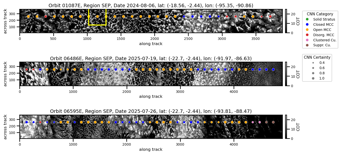
Figure 2 Three example MSI swaths of stratocumulus clouds, with the M-COP COT displayed in grey scale. Coloured dots show the classification into different cloud mesoscale structures by the CNN fine-tuned to MSI; positions of the dots are the midpoints of the classified cloud scenes; sizes of the dots encode the certainty value of the CNN. The yellow square in the upper panel shows the size of the 128 km × 128 km input scenes for the CNN.

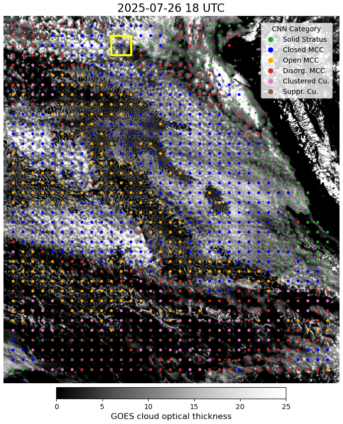
Figure 3 Example GOES/ABI image of the SEP stratocumulus region, with GOES COT displayed in grey scale. Coloured dots show the classification into different cloud mesoscale structures by the CNN fine-tuned to GOES; positions of the dots are the midpoints of the classified cloud scenes. The yellow square in the upper part of the image shows the size of the 128 km × 128 km input scenes for the CNN.

To apply the CNN to MSI and GOES, the input scene data must have a resolution of 1 km, i.e. the original MODIS resolution. To this end, the resolution of the MSI input scenes is reduced from 500 m to 1 km by a 2×2 average-pooling operation, and the GOES input scene data is interpolated from an original resolution of approximately 2 to 1 km by a weighted mean of nearby original values. The CNN is applied only during daytime. For MSI, this restriction arises because COT is unavailable at night. For GOES, nighttime COT proved incompatible with the network, likely due to fundamental limitations of infrared-only retrievals in capturing high COT values. We only consider scenes without overlying ice clouds. To this end, we check for each scene if there are brightness temperature values below 273 K, and disregard the scene if more than 5 % of the pixels within a scene have these low brightness temperatures. Besides the classification into cloud structures, the CNN provides a certainty value between 0 and 1 (see Wu et al., 2025 for details). We filter for cloud scenes that were classified with a certainty value >0.75, which is the case for about 67 % of both closed and open cell scenes.

To adapt the network to MSI and GOES, we produce two fine-tuned CNN versions, one for each imager. The fine-tuning is done for the final network layer using manually labeled cloud scenes. Approximately 500 scenes per instrument were labeled according to the six cloud structure classes. Parts of this dataset are withheld from training to evaluate model performance. After fine-tuning, the CNN shows substantially improved classification skill with an F1 score (a performance metric balancing precision and recall) of 0.86 and 0.9 for closed and open cells respectively for the CNN fine-tuned to MSI, and an F1 score of 0.88 and 0.94 for closed and open cells respectively for the CNN fine-tuned to GOES. A detailed evaluation of the fine-tuned CNNs for MSI and GOES is provided in the Appendix A. Examples of the resulting mesoscale cloud-structure classifications for MSI and GOES are shown in Figs. 2 and 3.

2.6 Putting it all together: Dataset of closed and open cell properties with transition information

The CNN fine-tuned to MSI is applied to MSI swaths in all four stratocumulus regions. Scene midpoints are spaced 64 km apart, resulting in overlapping scenes of 128 km (see Fig. 2). This overlap provides a finer structure detection, particularly near cloud structure boundaries. Due to this scene overlap, individual profiles are typically assigned to two neighbouring MSI scenes, and therefore sampled twice. For ACM-CAP, we compute the mean and coefficient of variation (CV = standard deviation $/$ mean) for different cloud and precipitation properties for each of these along-track 128 km scenes. For LWP and RWP, means and CVs are computed over all cloudy profiles; thus, they represent values conditional on cloud occurrence. For CTH, CBH, N_d, and r_e, scene-statistics are likewise computed over cloudy profiles, whereas D₀ scene-statistics are calculated only for raining profiles. Additionally, we define a binary rain occurrence for each scene, counting a scene as rainy if any of its profiles show rain. We also compute a rain fraction as the relative frequency of rainy profiles compared to cloudy profiles within a scene.

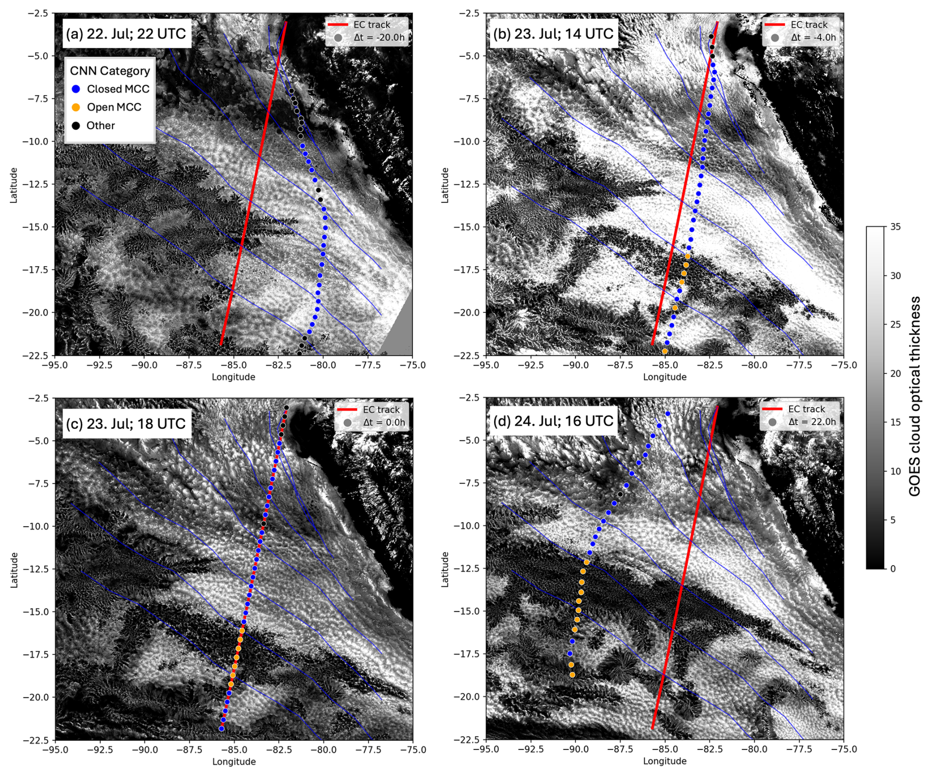
Figure 4 Example illustrating the method used to track cloud structure evolution along trajectories. The panels show GOES COT for four time steps between 22–24 July 2025. The red line shows the location of the EarthCARE overpass, which happened around 18:00 UTC on 23 July. Trajectories are initiated at the time of the EarthCARE overpass (c) and tracked backwards (a, b) and forwards (d) in time. The coloured dots represent the midpoints of each tracked cloud scene (128 km×128 km), with colours indicating the mesoscale cloud type retrieved by applying the CNN to the GOES imagery. Thin blue lines indicate the full trajectories for a subset of these scenes.

The resulting dataset contains scenes classified into one of the six mesoscale structure classes, including open and closed cells, and cloud property information from ACM-CAP per scene for all four stratocumulus regions. Overall, the dataset contains about 5000 scenes of closed cells, and about 2500 scenes of open cells. Figure 1 shows the geographic distribution of closed and open cells in the four stratocumulus regions, computed from this dataset. Closed cells occur most frequently in near-coastal regions, whereas open cells typically occur more offshore, consistent with previous findings (Muhlbauer et al., 2014; Mohrmann et al., 2021; Wu et al., 2025).

For the SEP region, we retrieve additional information about the temporal development of cloud structures around the EarthCARE overpasses. To this end, we apply the CNN to GOES imagery along the computed wind trajectories. More specifically, we interpolate the trajectories to a temporal resolution of two hours and use the corresponding GOES data for 128 km × 128 km scenes around the position of each trajectory. We then apply the fine-tuned CNN to these scenes to determine the cloud structure. Figure 4 illustrates this approach for a single EarthCARE overpass. An animation of this example, showing all time steps, is provided in the Video Supplement (Mayer, 2026a, https://doi.org/10.5446/73703).

Figure 5 All trajectories for which closed-to-open cell transitions were found. (a) Trajectories for cloud scenes that were closed cells at the time of the EarthCARE overpass and later transitioned to open cells; (b) trajectories for open-cell scenes at time of the EarthCARE overpass that could be traced back to a transition from closed cells at an earlier time. Dots mark positions of scenes at EarthCARE overpasses; crosses mark positions of transitions. The color encodes the time difference between overpass and transition.

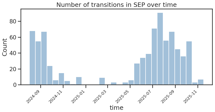
Figure 6 Number of closed-to-open cell transitions identified in the combined EarthCARE-GOES dataset as a function of time.

For each tracked cloud scene, we identify whether a transition from closed to open cells occurs and record the timing of this transition. In the example in Fig. 4, a pocket of open cells has formed by the time of the EarthCARE overpass at latitudes −15 to −20° (Fig. 4c). Using the trajectories, we trace the observed open cells back to the moment when they formed. Figure 4a, b shows, for example, that the pocket of open cells had not yet formed 20 h before the EarthCARE overpass and was smaller in size 4 h before the overpass. Conversely, some scenes are classified as closed cells at the time of the EarthCARE overpass, and transition to open cells later (in Fig. 4d due to the increasing size of the pocket of open cells). Again, we identify whether a transition occurs in these cloud scenes and determine its timing. As described in Sect. 2.5, the CNN classification for GOES is only available during daytime. For transitions occurring during nighttime – i.e. when a scene is classified as closed cells at the last available time of day 1 and as open cells at the first available time of day 2 – we pinpoint the time of transition using the brightness temperature of the 11.2 µm GOES channel: As cloud fraction is expected to decrease rapidly during a transition from closed to open cells, we define the time during the night when the change in brightness temperature is maximal as the transition time.

Overall, we find 803 trajectories for which transitions from closed to open cells occur; 330 of which are closed cells at the time of the EarthCARE overpass and transition to open cells at a later point in time, and 473 are open cells at the EarthCARE overpass and could be traced back to their previous closed-cell state. Figure 5 shows all of these trajectories. It shows that trajectories go, as expected in the SEP region, typically from South-East to North-West. Transitions were found throughout the studied region, with the majority being located relatively central to it. Figure 6 shows that transitions were mainly found during the time period from June to October, consistent with previous satellite observations that show that the frequency of occurrence of both closed and open cells is highest during these months (Muhlbauer et al., 2014).

Note that it is not feasible to estimate the time evolution of cloud scenes by collecting several EarthCARE overpasses along a trajectory (as was done e.g. by Eastman et al., 2022, for MODIS data), since the active instrument swath is narrow and very rarely coincides with the position of a trajectory more than once. Therefore, the approach of combining EarthCARE with GOES was chosen, which has the additional advantage that, due to the high temporal resolution of GOES, it is possible to pinpoint the timing of the transition to a narrow time range.

3 Results

3.1 Properties of closed and open cells

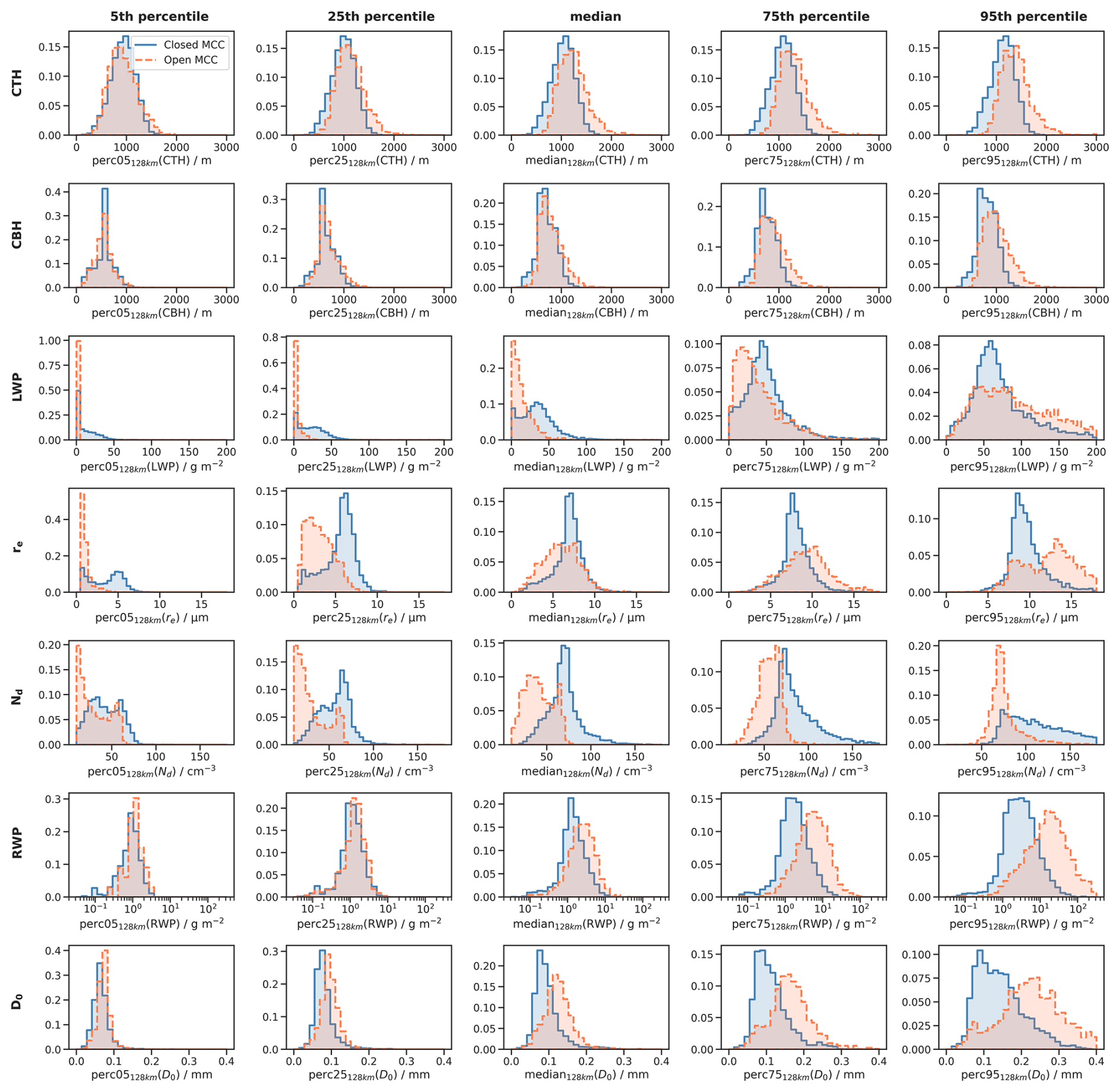
In this section, we analyse the similarities and differences between closed and open cells in terms of their cloud properties, as determined by ACM-CAP. To illustrate the cloud and rain products, and the variability withing cloud scenes, Fig. 7 shows example scenes of typical closed and open cells from ACM-CAP and M-COP. As described in Sect. 2.6, we compute the mean and CV of cloud and rain properties for each 128 km along-track cloud scene in ACM-CAP (see Fig. 7). The statistics of scene-mean and CV for all scenes from all stratocumulus regions are shown in in Fig. 8. In Appendix B, we additionally present statistics of the median, and 5th, 25th, 75th and 95th percentiles of all closed and open cell scenes, since mean and CV alone cannot capture all aspects of a distribution.

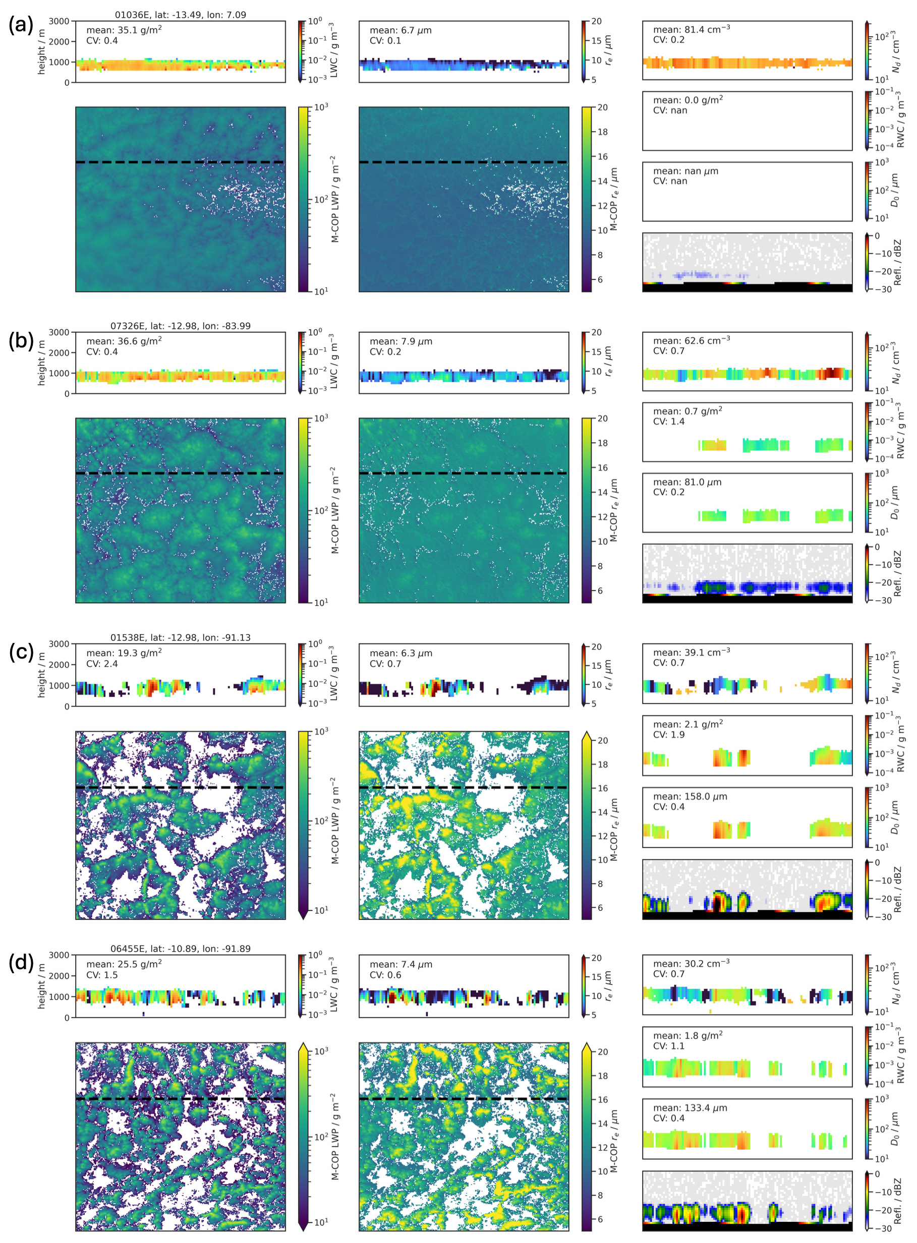
Figure 7 Examples of two typical closed-cell (a, b) and two typical open-cell (c, d) cloud scenes. Larger subplots show M-COP LWP and r_e for the four 128 km × 128 km scenes. The smaller subplots show the corresponding ACM-CAP profiles along-track (black dashed line in M-COP images) for several cloud and rain variables, namely liquid water content, r_e, N_d, RWC and D₀. The bottom right subplot shows the CPR reflectivity for each scene. The orbits and mid-points of the four scenes are specified in the titles. Numbers at the top left in ACM-CAP subplots are the mean and CV taken over the 128 km along-track scenes.

We start with analysing the vertical structure of clouds. EarthCARE's high vertical resolution and reduced surface clutter enable satellite-based measurements of the vertical structure that were difficult to obtain with previous missions. Figure 7 shows that the vertical extent in terms of average cloud base height (CBH) and cloud top height (CTH) is similar for the closed and open cell examples. It also shows that the CTH and CBH of the closed cells remain stable across the scene, whereas the open cells exhibit greater variability, with thin cloud layers existing between thicker cells. These thin cloud layers are usually found at the minimum CBH or maximum CTH level. This indicates that they may be new cells forming or remnants of old cells, respectively. The vertical structure features in the example scenes are typical of the overall statistics over all data in the four stratocumulus regions (see Fig. 8). The distributions of mean CTH and CBH show only small differences. Open cell CTHs are slightly higher (about 200 m on average), and this relatively small difference reduces even to 60 m, when stratifying by longitude and season for each stratocumulus region (not shown). The mean CBH difference between open and closed cells, when stratified by longitude and season, is only 10 m (not shown). The higher CV of both CBH and CTH reflects the highly variable vertical structure of open cells, which consists of thin layers interspersed with thicker cells. These findings on vertical structure broadly agree with previous findings from aircraft case studies (Wood et al., 2011).

Next, we analyse the cloud microphysical properties. The examples in Fig. 7 illustrate that the LWP is spatially more homogeneous for closed cells. In open cells it is much more variable, with LWP values significantly higher in some regions than in others. In the overall statistics (see Fig. 8), the mean LWP per scene is similar or slightly smaller for open compared to closed cells, but open cells have a higher CV, i.e. they have more “extreme” values of LWP, both smaller and larger (see also the low and high percentile distribution in Appendix B). A similar pattern can be seen with r_e: closed cells exhibit highly homogeneous r_e, whereas open cells demonstrate greater variability. While the mean r_e is similar for both cloud types, as with LWP, open cells exhibit greater variability and “extreme” r_e values. N_d on the other hand shows a large difference between closed and open cells in mean values, with open cells having very low N_d values of 10 to maximally 100 cm⁻³. The findings of similar LWP and lower N_d for open cells fit to previous satellite studies using passive imagers (Wood et al., 2008; Smalley et al., 2022). However, previous studies have often found larger average r_e in open cells, (e.g. Stevens et al., 2005; Rosenfeld et al., 2006; Wood et al., 2008; Watson‐Parris et al., 2021; Smalley et al., 2022), whereas we find that the average r_e value does not change but the variability of r_e gets larger with more large particles, but also more small particle sizes. A comparison with collocated M-COP retrievals shows that also EarthCARE's passive imager retrieves larger r_e in open cells, and that small r_e values in ACM-CAP occur mainly in optically thin parts of the open cells (Appendix C). These optically thin cloud layers are more readily detected by the ACM-CAP active-sensor synergy than by passive imagers, which preferentially sample the optically thicker parts of open cells and therefore retrieve larger average r_e.

A plausible physical explanation for the microphysical differences between closed and open cells comes from LES simulations (e.g. Wang and Feingold, 2009a; Chandrakar et al., 2022): In closed cells, there are typically many CCN available (as confirmed by aircraft measurements; Petters et al., 2006; Wood et al., 2011; Terai et al., 2014). Updrafts and high supersaturation lead to the activation of many droplets, which compete for water vapor. These droplets stay small in size and with a narrow droplet size distribution. In open cells, there are fewer CCN available due to rain scavenging. This leads to fewer cloud droplets, as well as to broader size distributions.

An interesting feature, that we see in many M-COP examples of non-precipitating closed cells, is the horizontal distribution of r_e within individual cloud cells: r_e is largest at the edges of the cells and smallest at the centre, where the updraft is located – even though the difference is small, it is consistent through many examples we analysed (see M-COP r_e in Fig. 7a as an example). An explanation might be that droplets are older in downdrafts than updrafts (de Lozar and Muessle, 2016; Chandrakar et al., 2022, who showed larger droplet ages in downdrafts for open cells) and might therefore have more time to grow to (slightly) larger sizes. For precipitating closed cells and open cells, the horizontal r_e distribution is reversed, with larger r_e at the positions of updrafts (see M-COP r_e in Fig. 7b–d).

Lastly, we analyse the rain properties. Open cells show a higher frequency of rain occurrence and higher RWP compared to closed cells, which fits well with smaller N_d, higher variability of droplet sizes and greater extremes in LWP (see Fig. 8). However, note that closed cells also drizzle in about 60 % of scenes, albeit often only lightly. More heavy rain (RWP > 20 g m⁻²) is rarely found in closed cells, but often occurs in open cells (see 95th percentile distribution in Appendix B). The rain fraction in Fig. 8 shows a broad distribution for both closed and open cells. Especially for open cells, the sampling nature of active instruments may be partly responsible for this broad distribution, since in some cases the satellite passes directly over the centres of raining cells; in other cases it may sample mainly cloud edges or optically thinner areas. For closed cells, the most common cases are only few raining profiles, i.e. rain fraction close to zero, and rain fractions close to one. Lastly, rain drops are larger in open cells (see Fig. 8). The size of raindrops has implications for virga depth and surface rain rates, since larger droplets are more likely to reach the surface. This, in turn, implies stronger aerosol scavenging. The higher CV of rain drop sizes is due to a higher number of large raindrops in open cells; small raindrop sizes are equally frequent in closed and open cells (see 5th and 95th percentile distribution in Appendix B).

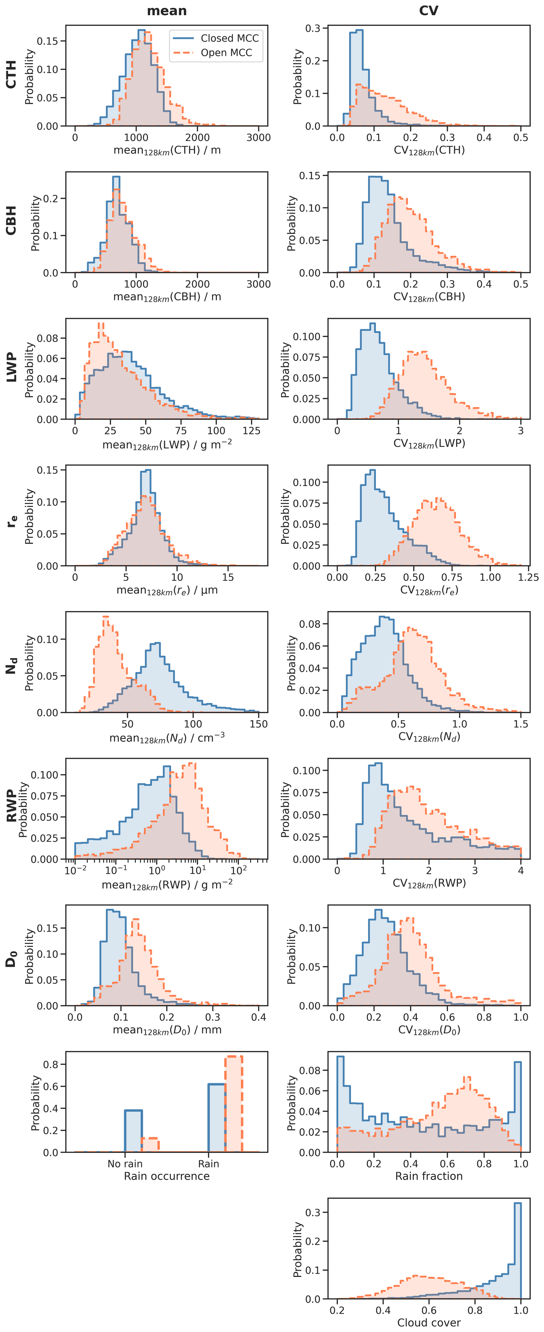
Figure 8 Probability distributions of cloud and rain properties of closed and open cells over all stratocumulus regions. For the upper seven rows, panels in the left column show the distribution of mean values over 128 km scenes; panels in the right column show the distribution of CVs. The lowermost two rows show rain occurrence, rain fraction for raining scenes, and cloud cover.

Higher rain rates in open cells compared to closed cells have also been found in previous studies using CloudSat and AMSR/E (Muhlbauer et al., 2014; Eastman et al., 2022), as well as ground based measurements (Jensen et al., 2021) and aircraft campaigns (Wood et al., 2011; Terai et al., 2014). The bigger surprise is the high rain occurrence in closed cells, which have in the past often been considered as non-raining. This notion may stem from the fact that most field studies have sampled clouds relatively close to the coast with small CTHs and consequently lower probability of rain, as shown by Possner et al. (2020). EarthCARE's high sensitivity enables the rain properties of low-level clouds to be quantified and studied in great detail for the first time from a satellite. As mentioned in Sect. 2.1, EarthCAREs drizzle detection is highly improved and able to detect even light drizzle, that might have gone undetected before. Our finding that (light) drizzle is prevalent in closed cells, is to a large extent thanks to this improved sensitivity (Xu et al., 2026). It should be noted here that, as the other variables, the frequency of rain is computed on a scene basis, i.e. a scene is counted as raining if at least one profile within the 128 km scene shows rain. This may lead to higher values for rain occurrence in closed cells with sparse precipitation than if we were to count rain profiles in the original 1 km resolution. However, Fig. 8 shows that high rain fractions are also relatively common in closed cells, and we believe that scene-based rain occurrence is a more relevant measure for capturing mesoscale cloud properties. The measurement of rain drop sizes, D₀, are also strongly improved for EarthCARE: The Doppler measurements are strongly dependent on particle sizes, and therefore help to determine both rain rates and drop sizes (Mason et al., 2017, 2023).

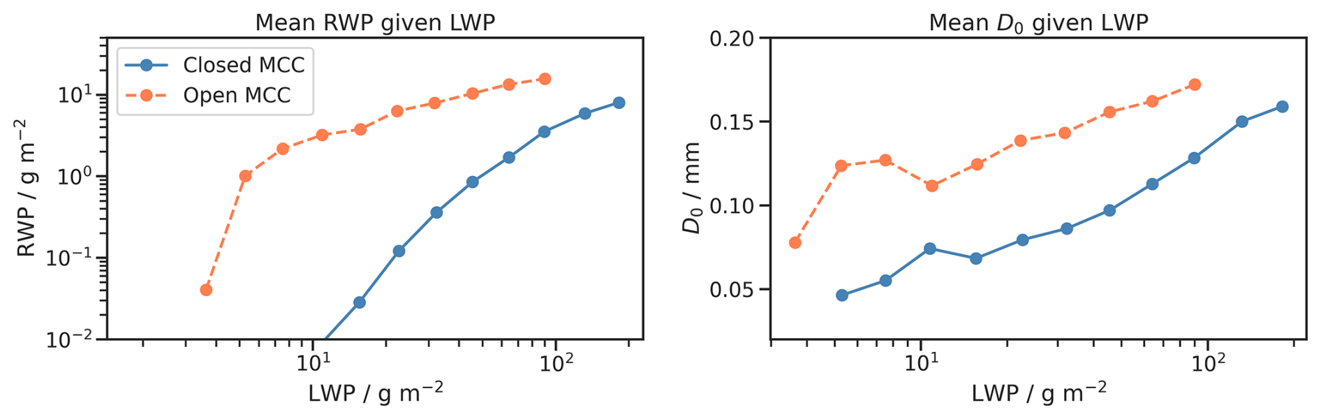
Figure 9 Mean RWP and D₀ per LWP bin for closed and open cells. The mean is computed over all four stratocumulus regions.

As described above, closed and open cells exhibit similar mean LWP, yet open cells show substantially larger RWP. This indicates that the LWP-RWP relationship differs between the two cloud regimes, as examined in Fig. 9. For a given LWP, open cells consistently produce higher RWP than closed cells, implying a markedly greater efficiency in rain formation. This behavior is robust across all four stratocumulus regions analysed. The enhanced RWP in open cells is primarily driven by larger raindrop sizes rather than by increased raindrop number concentrations. These statistics align with observations of individual cases: we find open-cell examples exhibiting intense precipitation even at low LWP, including instances where RWP exceeds LWP (e.g., the left-most and central cells in Fig. 7c). Such cases likely represent decaying cells in which a substantial fraction of cloud water has already been converted into rain. Similar phenomena have been reported in airborne observations by Wood et al. (2011).

Summarizing, EarthCARE provides detailed observations on vertical structure and microphysics of cloud and rain for closed and open cells. The two cloud structures show large differences in their microphysics, most notably lower N_d and stronger rain in open cells.

3.2 Transitions from closed to open cells

A polar-orbiting satellite such as EarthCARE provides only instantaneous measurements of cloud properties at the time of overpass. As described in Sect. 2.6, we combine these instantaneous observations with backward and forward trajectories, as well as GOES/ABI geostationary imagery, to reconstruct the temporal evolution of individual cloud scenes, especially their time to transition (= time of EarthCARE overpass − time of transition from closed to open cells). This analysis focuses on the SEP region, where most transitions between open and closed cells occur.

To illustrate clouds and their properties around the transition time with an example, Fig. 10 shows M-COP and ACM-CAP variables for an overpass section consisting of four neighboring, overlapping cloud scenes (grey lines in uppermost panel). Clouds in the left two scenes have (mostly) transitioned to open cells shortly before (1 h) the overpass, and the clouds in the right two scenes transition to open cells shortly after (1 and 3 h respectively) the overpass, as determined by tracking them in GOES. Note the large r_e, low N_d and high RWC in the closed cells, compared to typical non-transitioning closed cells as shown in Fig. 7. More example scenes, ordered by their time to transition, can be found in Appendix D.

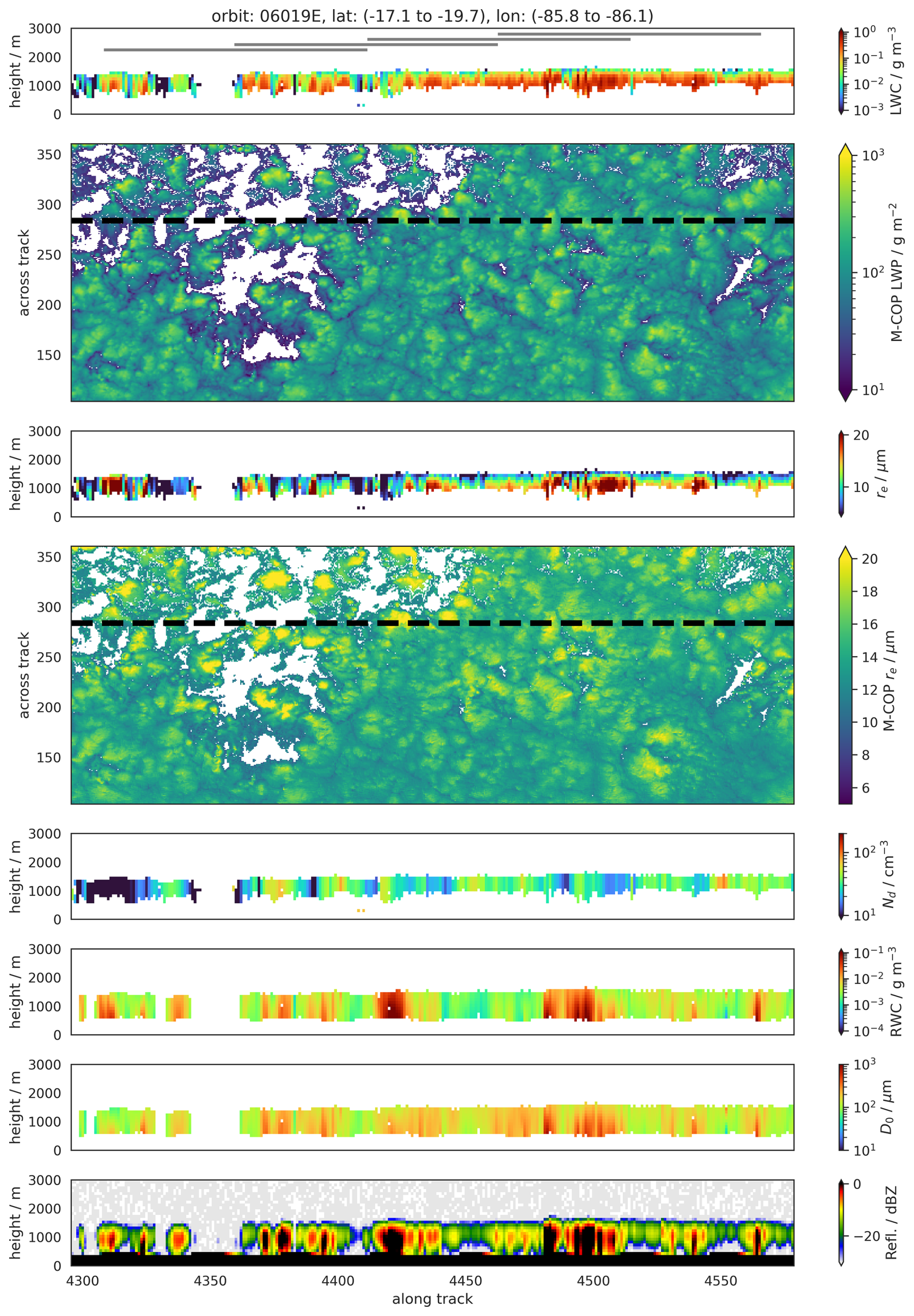
Figure 10 Example illustrating cloud and rain properties from M-COP and the corresponding ACM-CAP section along-track (black dashed line in M-COP images), together with CPR reflectivity, for clouds shortly before and after transition to open cells. The figure consists of four neighbouring cloud scenes, whose extent along track is shown by the grey lines in the uppermost panel. For the leftmost two scenes, much of the cloud field had transitioned to open cells shortly (1 h) before the overpass, whereas on the right, transition occurred shortly afterward (1 and 3 h for the two scenes respectively).

Figures 11 and 12 present all cloud scenes in which closed-to-open cell transitions were identified. The figures show cloud and rain properties retrieved from EarthCARE, plotted as a function of their time to transition. Figure 11a shows the number of cloud scenes that were found for different time-to-transition values. The EarthCARE overpass, and therefore the time of measurement, is always around 13:00 LT (local time) in the SEP region. Different time-to-transition values therefore mean that the transition happened at different times of the day. A first observation to note in Fig. 11a is that transitions were found at almost all time-to-transition values, hence transitions can happen at any time of the day. A transition occurring between 5 to 19 h before or after the overpass, means local nighttime. Adding all transition counts during daytime and nighttime in Fig. 11a shows that the majority of transitions occur during nighttime (around 60 %), consistent with Wood et al. (2008). Furthermore, the number of transitions show an interesting pattern with peaks at dawn (e.g. a time to transition of −19 means that a transition to open cells happened 19 h after the EarthCARE overpass, hence around 08:00 LT. A time to transition of 5 means that the transition to open cells happened 5 h before the EarthCARE overpass, i.e. again around 08:00 LT). Figure 11b shows cloud cover, derived from M-COP. As expected, cloud cover is near unity for closed cells and drops to much lower values, around 0.6, after clouds transition to open cells. Both CTH and CBH remain relatively constant and do not show notable deviations from their climatological values around the transition time. Their CV remain stable until the transition and increase around the transition time to higher values typical for open cells (dashed line in Fig. 11b).

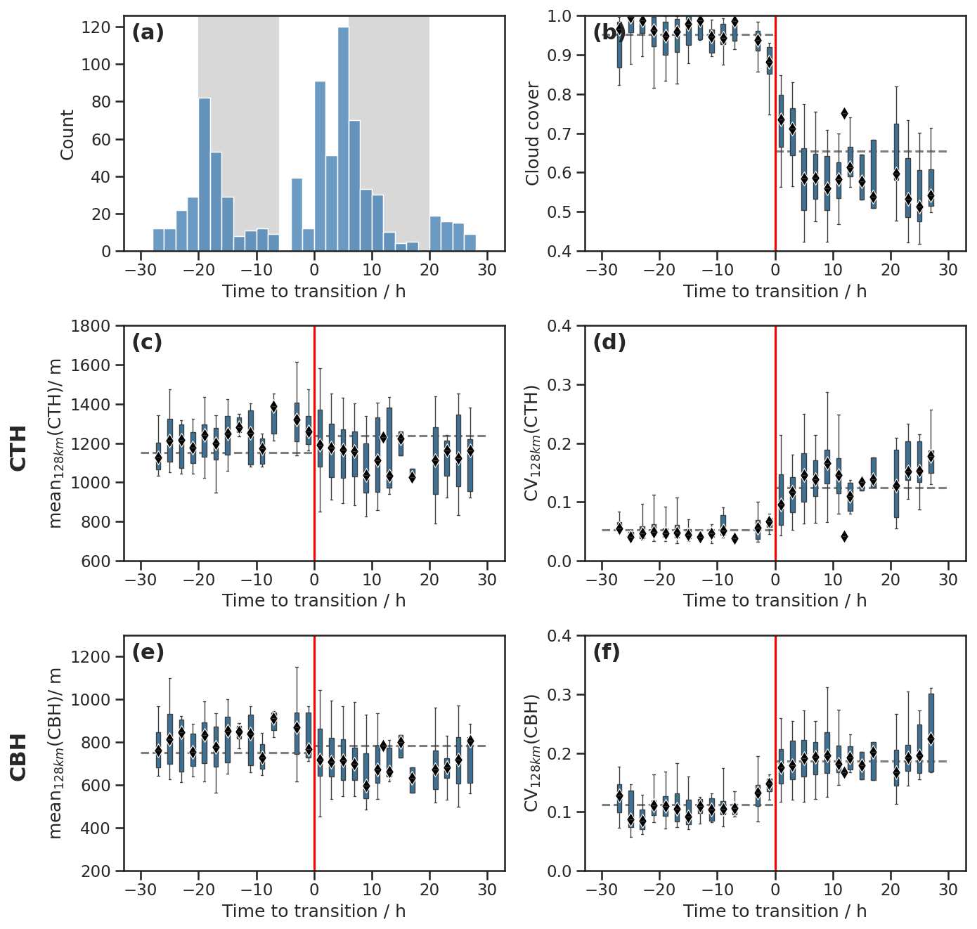
Figure 11 Cloud properties of all cloud scenes in which closed-to-open cell transitions were identified, as a function of their time to transition (= time of EarthCARE overpass − time of transition; determined from GOES morphology along trajectories). Negative time-to-transition values correspond to clouds that were still closed cells during the EarthCARE overpass and transitioned subsequently, while positive values correspond to scenes that had already transitioned prior to the overpass and could be traced back to an earlier transition time. (a) number of cloud scenes that were found for different time-to-transition values. Grey shading indicates that the transition happens during local nighttime. (b) cloud cover computed from M-COP; (c)–(f) cloud vertical structure from ACM-CAP. The box plots in (b)–(f) represent the distribution of mean_128 km and CV_128 km values of cloud parameters for all scenes with the same time-to-transition. Black diamonds indicate the medians of these distributions. The blue bars indicate the values between 25th and 75th percentile, whiskers are from 5th to 95th percentile. Horizontal dashed, grey lines indicate the “climatological” median values for closed and open cells, derived from the closed and open cell distributions in Fig. 8. These serve as a reference for comparing with the medians of the box plots (i.e. of the cloud scenes for which transitions were identified).

Figure 12 Same as Fig. 11b–f, but for cloud microphysical and rain properties from ACM-CAP.

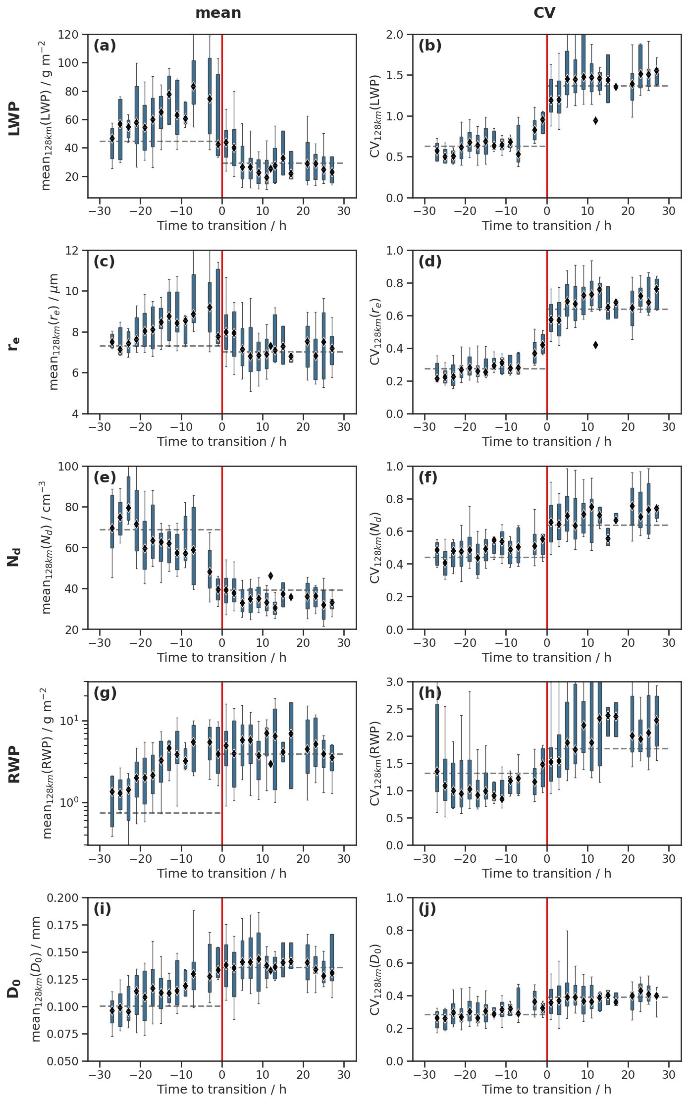
In contrast, LWP, r_e and N_d show a distinct temporal evolution already long before the transition (see Fig. 12a–f). LWP begins to increase approximately 25 h before the transition, peaks near the transition time, and subsequently decreases as open cells form – consistent with the emergence of thinner cloud layers characteristic of open-cell structure. In parallel to LWP, r_e increases with a peak shortly before the transition and decreases thereafter. As for LWP, the decrease is consistent with the emergence of thin cloud layers with small droplet sizes between the thicker open cell clouds. N_d steadily decreases toward the low climatological values of open cells. For both r_e and N_d, the deviations from their climatological closed-cell values seem to begin slightly later than for LWP, around 20 h before the transition. However, since the number of observed cases at these time-to-transition values are few (see Fig. 11a), it is difficult to draw a definite conclusion about the exact timing. The CV for LWP, r_e and N_d is relatively stable around the climatological values for closed cells and increases only shortly before the time of the transition. Hence, although the mean values of cloud microphysical parameters begin to change well before a transition occurs, they remain relatively homogeneous, i.e. at CV values typical of closed cells. It is only around the time of the transition that they begin to show stronger variations.

As with cloud microphysics, changes in rain properties occur well before the transition. RWP is already slightly elevated approximately 25 h before transition and increases to near open-cell climatological values approximately 10 h before the transition. In contrast to r_e and N_d, which show the strongest rates of change shortly before the transition, the increase in RWP slows down from around 10 h before the transition. D₀ steadily increases toward the higher climatological values of open cells. This increase of D₀ seems to begin a few hours later than for RWP, around 20 h prior to the transition, following a similar timeline as changes in r_e and N_d. However, as mentioned above, the precise timing should be viewed with a degree of caution and is more speculative than the overall quite clear trend.

Because increases in RWP (defined as mean_128 km(RWP), where the mean is taken over all cloudy profiles, as explained in Sect. 2.6 and shown in Fig. 12g) may have multiple origins, we decompose it in Fig. 13 into rain fraction (i.e. relative frequency of raining profiles compared to cloudy profiles) and mean${}_{\mathrm{128}\mathrm{km}}^{\mathrm{raining}}$(RWP), where the scene-mean is only taken only over raining profiles, i.e. capturing the rain intensity. Both quantities show increased values before transition. This means that the increase in RWP is both due to higher rain intensities and more clouds producing rain. This decomposition further shows that the early increase of RWP (from around 25 until 15 h before transition) is mainly due to increasing rain fractions (Fig. 13a), whereas the subsequent increase in RWP (from around 15 h before transition) is mainly due to increasing rain intensity (Fig. 13b).

Figure 13 Decomposition of RWP in Fig. 12g, in (a) rain fraction, and (b) RWP where the mean is taken only over raining profiles (instead of over all cloudy profiles).

4 Discussion

4.1 Interpretation of the transition timeline

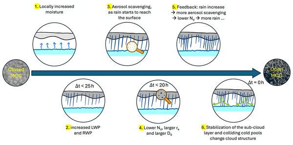
From the sequence of deviations from climatological values, we propose a timeline of physical processes leading to closed-to-open cell transitions (see Fig. 14). We hypothesise that the early increase in LWP and, as a consequence, RWP is due to increased moisture in the boundary layer – consistent with Eastman et al. (2022), who found that transitions are preceded (for lead times of ∼3 d) by strong surface winds that increase boundary layer moisture. Once rain intensifies and reaches the surface, aerosols in the boundary layer are scavenged, reducing N_d and increasing r_e as a consequence. This promotes further precipitation, sustaining a rain-aerosol-scavenging feedback. Increasing r_e also leads to larger D₀, which further intensify the rain-aerosol-scavenging feedback. After several hours, the rain and consequently the evaporative cooling below cloud base are strong enough to reorganise the mesoscale cloud structure into open cells through stabilization of the sub-cloud layer and colliding cold-pools. In this interpretation, enhanced moisture acts as a possible initial trigger, while aerosol scavenging provides an important positive feedback that intensifies precipitation and promotes breakup. Note that the the whole transition process following this timeline takes a long time; around 25 h.

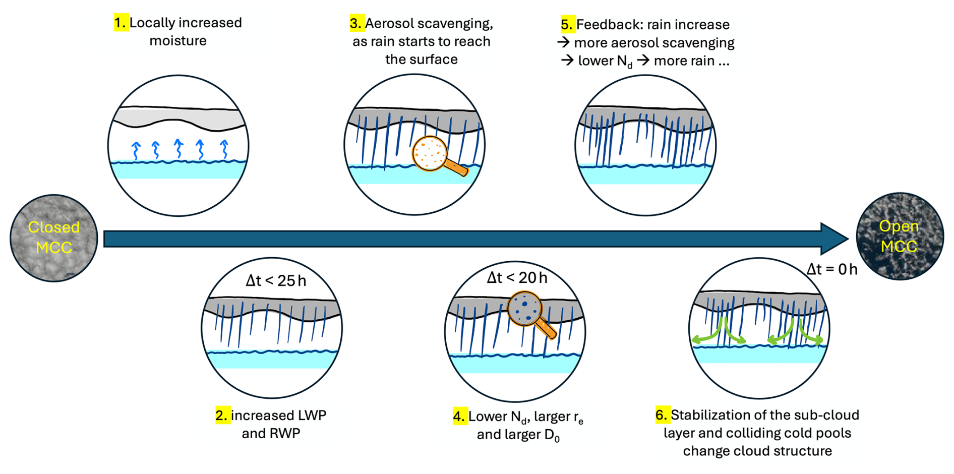
Figure 14 Hypothesised timeline for the processes leading to a transition from closed to open cells.

LES studies often use aerosol number concentration as a control parameter and show that low aerosol availability can favour open-cell conditions. Our observations are consistent with aerosol playing an important role, but suggest that low aerosol availability need not be the initial trigger of the transition: N_d is initially close to climatological values and decreases only after LWP and precipitation have already increased. This timing is consistent with aerosol depletion developing as part of the precipitation feedback rather than necessarily preceding it. Other upstream environmental controls, including SST and surface forcing, may contribute to the initial increase in boundary-layer moisture and precipitation (Sandu and Stevens, 2011; Yamaguchi et al., 2017), but quantifying their relative roles is beyond the scope of the present study.

The diurnal cycle of the number of transitions (see Fig. 11a) provides additional insight into the underlying processes. The observed peak in transitions around dawn may be linked to the diurnal evolution of LWP. In closed-cell stratocumulus, radiative cooling at cloud top is the primary driver of boundary-layer circulation. During nighttime, the absence of solar radiation enhances this cooling, leading to a gradual increase in LWP with a maximum near dawn. Given the close relationship between LWP and RWP, precipitation is also expected to peak at this time. This behaviour is consistent with our interpretation of a precipitation-linked transition pathway.

An open question is whether the onset of incoming radiation at sunrise also actively contributes to the transition. One possible mechanism is that shortwave radiation weakens the radiatively driven circulation of closed cells, thereby facilitating a shift toward open-cell dynamics. Assessing the relative roles of nocturnal cooling and daytime radiative effects in triggering transitions will require further dedicated investigation.

4.2 Implications

Our results, supported by previous work by Eastman et al. (2022), suggest that increased moisture in the boundary layer is a potential trigger for increased rain leading to a transition. This implies that changes in environmental conditions that increase boundary-layer moisture, for instance stronger surface winds and higher sea-surface temperatures, could lead to more open cell occurrences, decreasing the albedo and cooling effect of the stratocumulus decks.

Another implication is that high amounts of aerosols could delay or suppress rain formation, and consequently closed-to-open cell transition (Rosenfeld et al., 2006; Yamaguchi et al., 2017; Goren et al., 2019). This suggests that the recent trend of decreasing aerosol amounts may lead to a positive forcing (i.e. warming) through earlier transitions from closed to open cells along their trajectories.

4.3 Uncertainties and robustness

Our mesoscale cloud typing is based on a CNN applied to GOES and MSI imagers, and uncertainties in these classifications propagate into both the inferred contrasts between open and closed cells and the estimated time-to-transition. Manual inspection suggests a failure mode is the potential misclassification of dissipating or fragmented cloud scenes as open cells, which would bias the retrieved LWP and RWP low for the open-cell category. Another difficulty lies in scenes with clouds that are at the edge of transitions or breaking up (see Fig. 10). Here, the CNN usually classifies scenes as closed cells if more than half of the scene is covered by them, and vice versa for open cells. Therefore, the cloud and rain properties around the transition time may be partially derived from the other cloud regime covering part of the scene.

Note also that neural networks trained on different regions, seasons, or cloud scene sizes can encode systematically different notions of “open” and “closed” cells. In our case, the fixed scene size of 128×128 km limits detectability of very large cell sizes and may preferentially capture smaller-scale open cells. This scale dependence should be considered when interpreting differences with prior work.

In addition to classification uncertainties, uncertainties in the EarthCARE retrievals must also be acknowledged. These products are still maturing, and forthcoming retrieval updates may affect some variables, particularly the distribution of cloud and rain particles within the vertical profiles. For this reason, we focus on column-integrated cloud and rain properties that are more robust and additionally constrained by the passive MSI imager.

Please note that our study focuses on daytime retrievals only, since the current version of the fine-tuned CNN only operates during the day. Cloud properties may exhibit diurnal cycles, which could impact transition processes (Pugsley et al., 2025). However, this aspect is not addressed in our study. As mentioned above in Sect. 3.2, we observe a diurnal pattern in the number of transitions, with the majority occurring around dawn. Although the timing of transitions is more challenging at night, introducing an element of uncertainty into their distribution (see Sect. 2.6), this observation suggests that the diurnal cycle plays an important role in the transition process. A possible next step would be to incorporate night-time overpasses and study the effect of the diurnal cycle on closed and open cell properties and their transitions directly.

Further, the nature of active remote-sensing measurements may enhance the spread in our results. Depending on the exact satellite-ground track position relative to the mesoscale cloud structure, EarthCARE may sample different parts of the same cloud regime. In some cases, the satellite passes directly over the centres of cells or over regions of strong precipitation; in other cases – particularly for open-cellular scenes – it may sample mainly cloud edges or optically thinner areas. These geometric and structural differences naturally produce variability in the measured quantities. Such scene-dependent sampling differences are therefore expected to contribute to the overall dispersion in the data.

Finally, we would like to comment on the spread in many of the variables in the time series plots (Figs. 11, 12 and 13). This spread is often substantial relative to the magnitude of the detected trends. Therefore, one might argue that caution should be exercised when interpreting the observed trends. However, it should be noted that transition detection as well as time-to-transition estimation are performed independently for each cloud scene. The fact that smooth and coherent trends emerge despite this independence strengthens our confidence that the observed signals are physically meaningful.

4.4 Generality across regimes

Our analysis targets clouds in the subtropics and focuses on cloud and rain microphysics, since observations and theory suggest that the closed-to-open cell transitions are mainly driven by microphysical processes instead of large-scale meteorological conditions (Wood and Hartmann, 2006; Comstock et al., 2007; Bretherton et al., 2010; Berner et al., 2013; Glassmeier and Feingold, 2017; Smalley et al., 2022; Hoffmann et al., 2023). While we expect the microphysical processes as discussed in this work to hold in every situation, meteorological factors can still be of crucial importance in changing the initial cloud conditions or the timeline of transitions, for example by facilitating or hindering the development of rain. Eastman et al. (2022) found that increased wind speeds are associated with the development of open cells, which is consistent with our interpretation of increased moisture as a trigger for transitions. McCoy et al. (2017, 2023) found that a stronger instability, i.e. weaker boundary layer inversion strength, is associated with an increasing frequency of open cells. They show that this effect is strongest in mid and high latitudes, suggesting that the relative importance of precipitation feedbacks versus large-scale forcing is likely regime-dependent. Nevertheless, they still find a pronounced effect also in the subtropics. In future work it would be interesting to check the dependence of the transition timeline studied here on meteorological factors, like the inversion strength or sea surface temperature, to better understand how closed-to-open cell transitions might change in a changing climate.

5 Conclusions

This study utilizes the newly launched EarthCARE satellite to provide unprecedented insights into the properties of closed and open stratocumulus cells and the processes driving transitions between them.

EarthCARE has several advances compared to previous satellites that make it well suited to study low-level clouds. The combination of active (ATLID and CPR) and passive (MSI) sensors on the same platform enables simultaneous measurement of cloud mesoscale structure and detailed observations below cloud top. The CPR instrument is more sensitive than previous spaceborne radars, like CloudSat, and equipped with Doppler capabilities. This enables EarthCARE to overcome previous CloudSat limitations caused by ground clutter, better constrain rain and cloud retrievals and to detect even weak drizzle and small raindrops. Advanced retrieval techniques, like the optimal estimation algorithm of the ACM-CAP product, make use of the synergy of three instruments and are able to retrieve cloud and rain properties in unprecedented detail.

By applying a convolutional neural network to MSI data, we classify cloud mesoscale structures and analyse their microphysical properties using EarthCARE's synergistic measurements for a timespan of more than 15 months. Our results show that open cells differ markedly from closed cells especially in terms of microphysics. Open cells exhibit lower droplet number concentrations and more variable droplet sizes and liquid water paths. They have a higher frequency of rain occurrence, even though it should be noted that also closed cells rain in about 60 % of the cases. The larger difference is that open cells rain more heavily. They are notably more efficient at producing large rain amounts for a given liquid water path, primarily due to larger raindrop sizes.

To investigate the mechanisms behind closed-to-open cell transitions, we combine EarthCARE observations with GOES/ABI geostationary imagery and ERA5-driven wind trajectories. This approach allows us to track the evolution of cloud properties around closed-to-open cell transitions. We find that liquid water path and rain amounts in closed cells start to deviate from their climatological values up to 25 h before a transition, followed closely by a decrease in droplet number concentration and an increase of droplet sizes. The vertical cloud structure remains largely unchanged during this period.

Taken together, these findings support a precipitation-linked pathway to the closed-to-open transition, consistent with the conceptual picture developed from LES studies (Savic-Jovcic and Stevens, 2008; Wang and Feingold, 2009a; Feingold et al., 2010). The observed sequence is consistent with a feedback loop in which increased boundary-layer moisture enhances liquid water path and precipitation, leading to aerosol scavenging, reduced droplet number concentrations, and further precipitation intensification. An important point from the observed timeline is that the microphysical changes and gradual intensification of rain occur over a relatively long period of around 25 h before ultimately leading to a transition. This is consistent with previous work from Eastman et al. (2022), who find that closed-to-open cell transitions are preceded by strong winds and high latent heat flux for lead times of ∼3 d followed by microphysical cloud changes on timescales of 12–24 h.

We observe a pronounced diurnal cycle in the transition probability, with peaks occurring at dawn. This suggests that radiative cooling, leading to a gradual increase in cloud and rain water during the night, is an important part of the transition process, facilitating the formation of heavy rain necessary for open cell formation.

The new capabilities of EarthCARE enable high-sensitivity, fully collocated observations of cloud microphysics and precipitation, overcoming key limitations of previous satellite studies. A particular strength of this work is the synergy between these detailed EarthCARE retrievals and the high temporal resolution of GOES. This combination allows us to track the evolution of cloud properties around transitions with unprecedented detail, enabling the reconstruction of a physically coherent timeline of the microphysical processes governing closed-to-open cell transitions.

Nevertheless, several limitations should be acknowledged. Uncertainties arise from the CNN-based cloud classification, the use of ERA5-driven trajectories, and the EarthCARE retrievals, which, although advanced, are still maturing. The analysis is further limited to daytime conditions and subtropical regions. While robust temporal trends emerge across many transitions, the substantial variability indicates that additional factors, such as meteorological conditions, also influence the transition pathway.

Our results provide observational evidence that closed-to-open cell transitions are closely linked to precipitation-driven processes operating over timescales of about one day. This highlights the importance of representing aerosol-cloud-precipitation interactions in models to capture stratocumulus organization and its evolution. Because transitions from closed to open cells reduce cloud fraction and albedo, factors that modulate boundary-layer moisture or aerosol loading – such as changes in large-scale circulation, sea surface temperature or anthropogenic emissions – may strongly influence the radiative effect of marine stratocumulus.

Overall, this study demonstrates the power of EarthCARE's synergistic measurements for advancing our understanding of stratocumulus clouds and their controlling processes, and provides new observational constraints to improve the representation of stratocumulus clouds and their feedbacks in weather and climate models.

Appendix A: Fine-tuning of the CNN

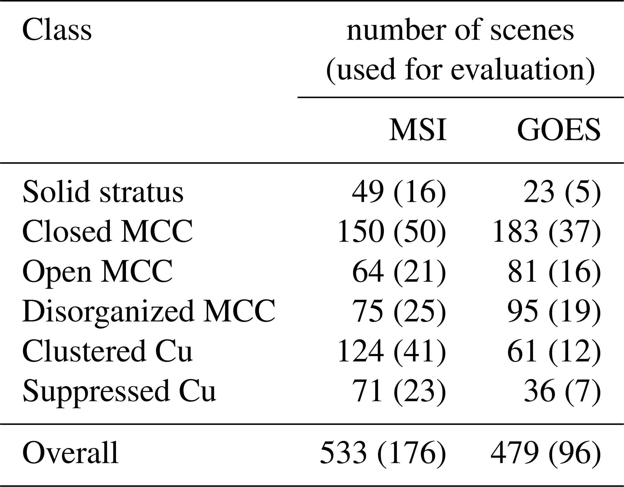
To adapt the CNN of Wu et al. (2025) to MSI and GOES imagery, we fine-tune the model using manually labeled cloud scenes. In total, 533 MSI scenes and 479 GOES scenes are labeled according to the six mesoscale structure classes (solid stratus, closed MCC, open MCC, disorganized MCC, clustered cumulus, and suppressed cumulus). For MSI, the labeled scenes are randomly drawn across all times and all four subtropical stratocumulus regions (SEP, NEP, SEA, and NEA), whereas GOES labels are drawn from the SEP region. Because of the natural variability of the occurrence of the different mesoscale structures, some structures are sampled more often than others (see Table A1), with closed cells being the most frequent cloud structure. Fine-tuning is applied only to the final network layer and performed using the torch.optim.Adam optimizer. To identify an optimal fine-tuning configuration, we conduct a hyperparameter grid search over learning rate, batch size, and number of epochs (learning_rate ∈ $\mathrm{5}\times {\mathrm{10}}^{-\mathrm{5}}$, 10⁻⁴, $\mathrm{5}\times {\mathrm{10}}^{-\mathrm{4}}$, batch_size ∈ 4, 8, 16, num_epochs ∈ 15, 20, 30). Part of the labeled dataset is withheld from training and used exclusively to evaluate model performance (see Table A1).

Table A1 Number of manually labeled cloud scenes for MSI and GOES per mesoscale cloud structure class. The number of scenes withheld from traning and used for evaluation is displayed in parenthesis.

A1 Evaluation of the fine-tuned CNN for MSI

Performance is quantified for both the fine-tuned and the original model to get an estimate of the models improvement due to fine-tuning. The confusion matrix in Fig. A1 shows how the performance of the CNN changes after fine-tuning: Most of the cloud structure classes have a higher accuracy, especially open-cell detection is strongly improved. Table A2 shows the average performance of the models over all cloud classes, using two different methods of averaging. It shows that the average performance is improved for the fine-tuned model by about 13 % to 14 %. Since our analysis focuses on stratocumulus mesoscale cellular convection, we emphasize performance for the closed- and open-MCC classes, which both show improvements in precision and recall. This can be quantified in the F1 score: closed cells have an F1 score of 0.86 in the fine-tuned and 0.76 in the original model; open cells have an F1 score of 0.9 in the fine-tuned and 0.5 in the original model. Overall, fine-tuning substantially improves MSI classification performance, most notably for open MCC, where both per-class accuracy and F1 score increase markedly relative to the original model.

Table A2 Overall classification performance for MSI on the validation dataset (176 scenes) for the CNN fine-tuned to MSI and the original CNN. Overall accuracy is the average accuracy over all cloud structure classes; equally-weighted accuracy takes into account that the classes have different numbers of samples.

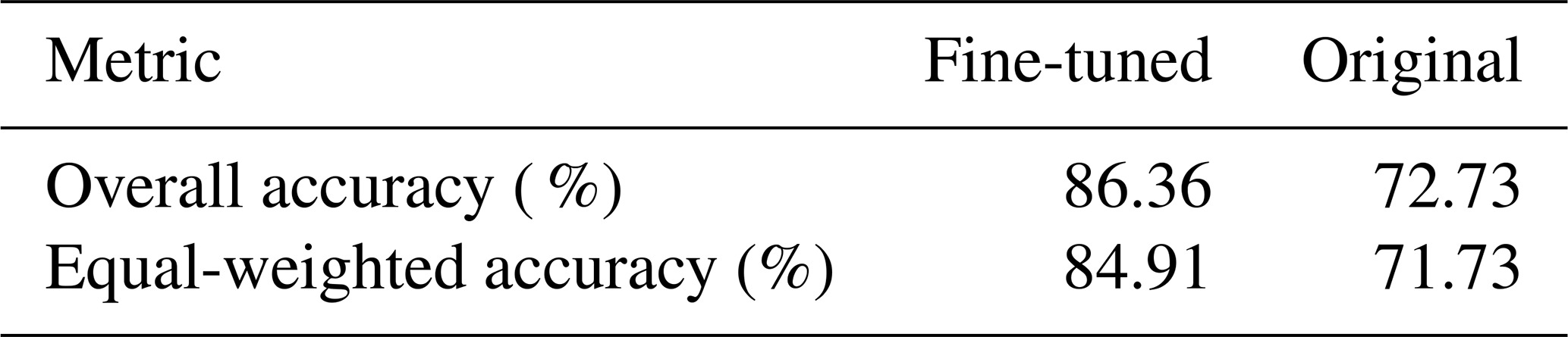
Figure A1 Confusion matrix for the performance of original CNN applied to MSI, and the CNN fine-tuned to MSI applied to the same scenes.

A2 Evaluation of the fine-tuned CNN for GOES

We evaluate the GOES fine-tuned CNN analogously. Performance is summarized using the same metrics as for MSI, and we again compare against the original model evaluated on the identical validation dataset. Per-class accuracy is strongly improved, especially also for closed and open cells (see Fig. A2). The solid stratus class shows worse performance after fine-tuning, however, in the manually labeled dataset for GOES there were only very few samples of this class (see Table A1), and the evaluation is therefore more uncertain than for other cloud structure classes. The average performance shown in Table A3 shows a strong average improvement for the fine-tuned model between 13 % and 26 %, depending on which measure is used. The F1 scores for closed cells are 0.88 for the fine-tuned and 0.63 for the original model; the F1 scores for open cells are 0.94 for the fine-tuned and 0.58 for the original model, showing that the balance of precision and recall is highly improved after fine-tuning.

Table A3 As Table A2, but for GOES.

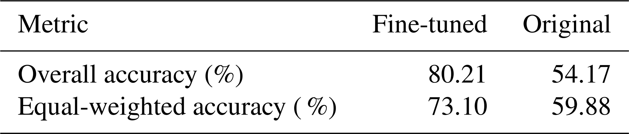
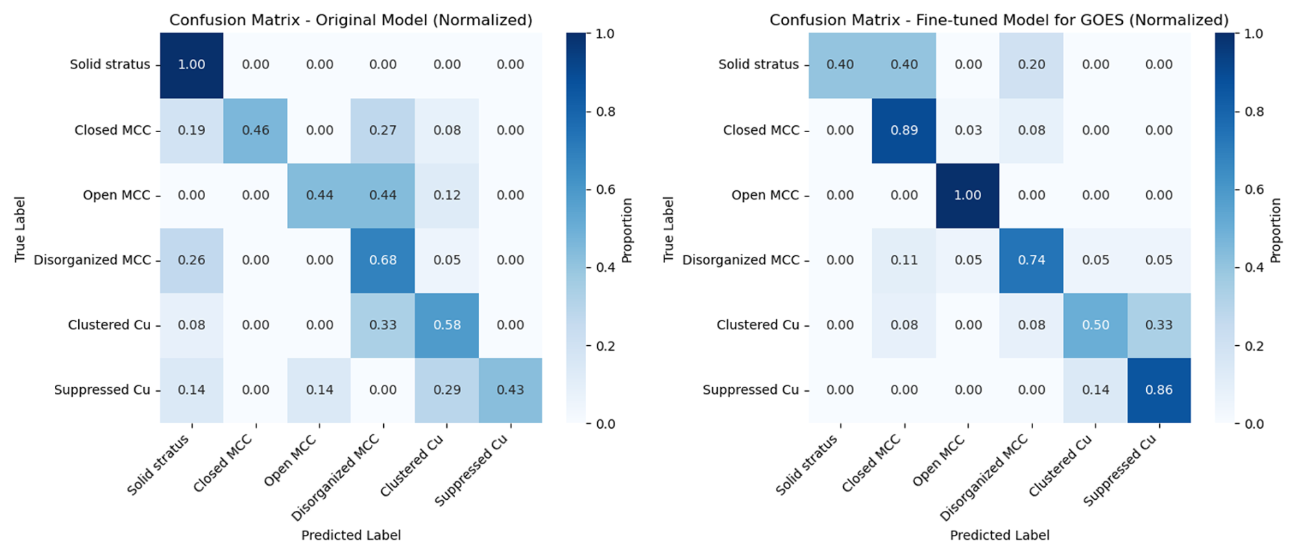
Figure A2 Confusion matrix for the performance of original CNN applied to GOES, and the CNN fine-tuned to GOES applied to the same scenes.

Appendix B: Properties of closed and open cells – percentiles

As a complement to Fig. 8, Fig. B1 illustrates additional aspects of the distributions of cloud and precipitation properties for closed and open cells. Shown are the 25th percentile, median, and 75th percentile for each variable, computed over 128 km cloud scenes using ACM-CAP retrievals. These percentile-based statistics highlight differences in distribution shape and variability that are not fully captured by the mean and CV alone.

Figure B1 Same as Fig. 8, but for percentiles and median per cloud scene.

Appendix C: Comparison with M-COP effective radius

To investigate where the discrepancies between our findings of similar average r_e for closed and open cells and previous findings of larger r_e in open cells originate, we compare ACM-CAP with collocated M-COP retrievals for June–August 2025. For each ACM-CAP profile, the M-COP pixel with the closest longitude–latitude position along track is selected. When all cloud profiles are included, ACM-CAP shows similar scene-mean r_e for open and closed cells, whereas M-COP retrieves larger r_e in open cells, consistent with previous studies using passive imagers (Fig. C1a).

The absolute r_e values are also shifted between ACM-CAP and M-COP. This offset can partly arise from differences between the retrieval methods of the still-maturing products. In addition, passive bispectral retrievals are weighted toward the upper part of the cloud, whereas the ACM-CAP values considered here are averaged over the cloud column. Since r_e generally increases with height in approximately adiabatic clouds, this difference in vertical sampling is expected to contribute to larger r_e from M-COP.

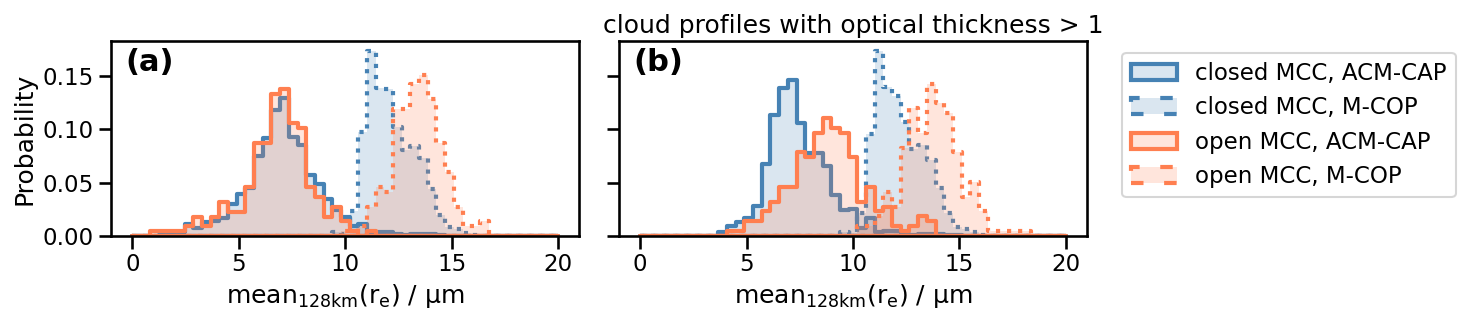
Figure C1 Probability distributions of scene-mean r_e for closed and open cells from ACM-CAP and collocated M-COP retrievals for June–August 2025. (a) All cloud profiles. (b) Taking only profiles with ACM-CAP cloud optical thickness >1 into account for the scene-means.

When only profiles with ACM-CAP optical thickness >1 are retained before scene averaging, the open-cell ACM-CAP distribution shifts toward larger r_e, while M-COP changes comparatively little (Fig. C1b). This suggests that the small ACM-CAP r_e values occur predominantly in optically thin parts of open-cell scenes that are less readily detected by passive imagers. Consequently, passive retrievals preferentially sample the optically thicker parts of open cells, where r_e is larger. Three-dimensional radiative effects and sub-pixel inhomogeneity, which are stronger for heterogeneous open-cell scenes, may additionally affect the retrieved r_e and contribute to differences between closed and open cells, as well as to retrieval differences between the two products (e.g., Zhang et al., 2012).

Appendix D: Examples of transitioning cloud scenes

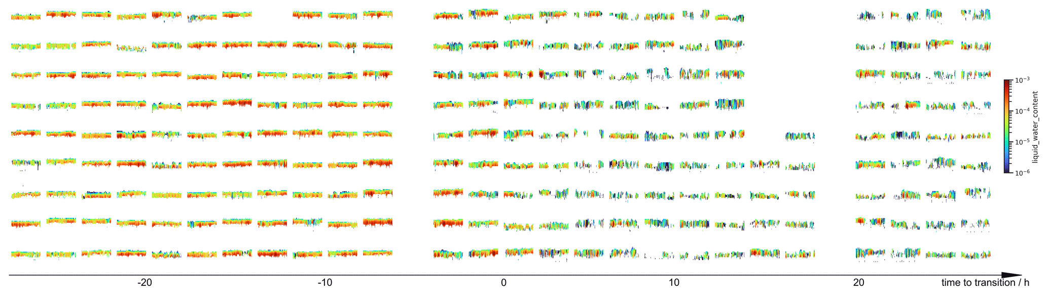
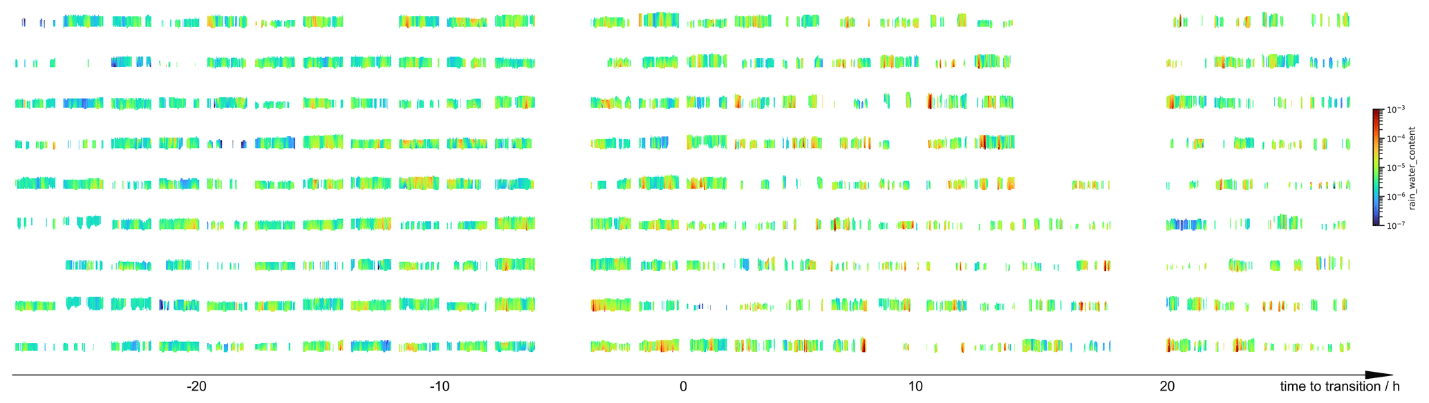
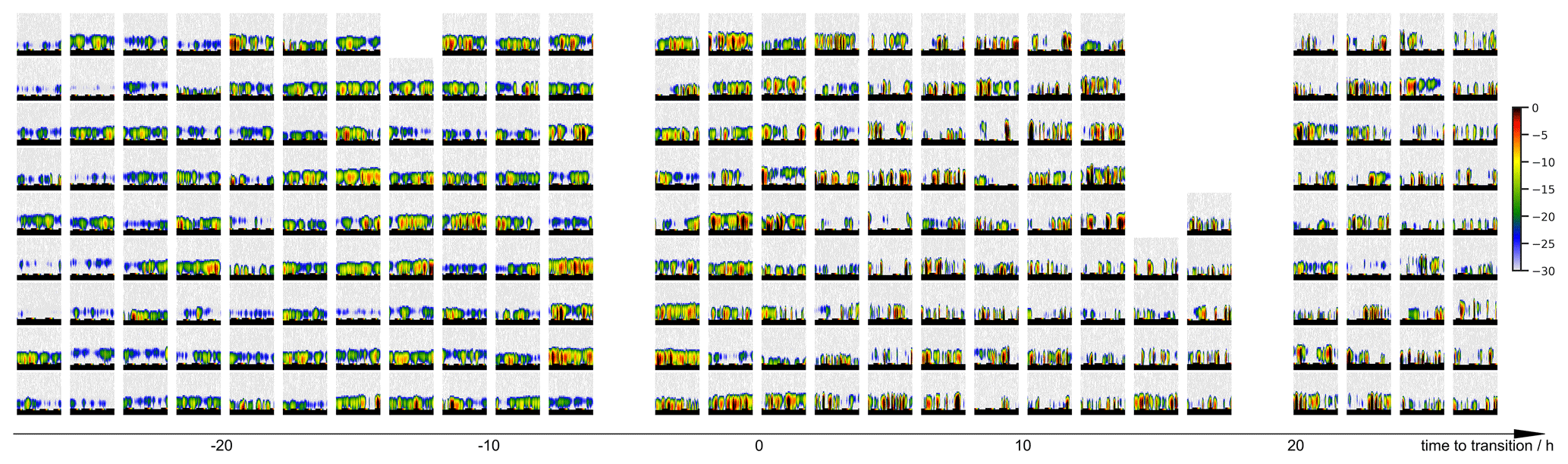
To illustrate the time evolution in cloud and rain properties around closed-to-open cell transitions, Figs. D1, D2, D3, and D4 show M-COP LWP, ACM-CAP liquid water content and RWC, and CPR reflectivity for example scenes for each time-to-transition value.

Figure D1 M-COP LWP for example cloud scenes for which closed-to-open cell transitions were identified. The scenes are ordered from left to right by their time to transition, using the same time-to-transition bins as in Figs. 11, 12 and 13. For each time to transition value, nine scenes were picked randomly. For some time-to-transition values less than nine scenes were found overall, and for time-to-transitions $=-\mathrm{5}$ and 19 h no corresponding scenes were found (see Fig. 11a).

Figure D2 Same as Fig. D1, but for ACM-CAP liquid water content. The scenes correspond to the ones shown in Fig. D1.

Figure D3 Same as Fig. D1, but for ACM-CAP rain water content. The scenes correspond to the ones shown in Fig. D1.

Figure D4 Same as Fig. D1, but for CPR reflectivity. The scenes correspond to the ones shown in Fig. D1.