Uncertainties in recent tropical stratospheric and tropospheric ozone changes limit the use of observational constraints for assessing future ozone change

A variety of chemical and dynamical processes in the troposphere and stratosphere affect tropical total column ozone (TCO), the net effect of which may cause changes in surface UV radiation and impact human and ecosystem health. We use dynamical linear modeling to estimate changes in tropical TCO and partial column ozone (PCO) in the troposphere and three stratospheric layers to assess agreement between satellite composites and chemistry-climate model simulations from two multi-model experiments (CCMI-1 and CCMI-2022). While both model experiments show tropical TCO increases over 2000–2021, multimodel-mean CCMI-2022 changes (+2.5 DU) agree slightly better with observations (+3.3 DU) than CCMI-1 (+1.6 DU). However, this overall agreement obscures multiple systematic differences in PCO changes between the models and observations across atmospheric layers. For example, since 2000 tropical tropospheric PCO increased significantly in CCMI-2022 (+1.5 DU) but not in CCMI-1 (+0.3 DU), largely explaining the difference in TCO changes. Also, despite nearly identical stratospheric PCO changes, CCMI-2022 changes are slightly more negative than CCMI-1 in the lower stratosphere (by ∼ 0.5 DU) and more positive in the middle/upper stratosphere. Crucially, substantial differences exist between observational PCO changes, particularly in the troposphere and middle/upper stratosphere, and these disagreements limit the ability to evaluate CCM fidelity for past changes. While early and late century trends are correlated across models, suggesting a potential emergent constraint on ozone, the spread in observational trends means they are unable to provide guidance on the credibility of model projections for a given emissions scenario.

1 Introduction

The amount of biologically harmful ultraviolet radiation reaching Earth's surface is strongly affected by the amount of total column ozone (TCO), and this motivates the need to understand both natural variability and anthropogenically-driven changes in TCO across a range of timescales. TCO includes contributions from ozone residing in the stratosphere (∼ 90 %, see Fig. 1) and the troposphere (∼ 10 %), and can vary due to a variety of chemical, physical, and radiative processes that are impacted by human activities.

In the 1970s and 1980s, reductions in stratospheric ozone from the emission of ozone depleting substances (ODS) became a topic of grave societal and scientific concern, and efforts to address this issue culminated in the adoption of the Montreal Protocol on Substances that Deplete the Ozone Layer and subsequent amendments. Because of the Montreal Protocol, the concentration of ODS has been declining in the atmosphere since around 1997, and ozone concentrations in the upper stratosphere and the Antarctic ozone hole are exhibiting signs of recovery (WMO, 2022). However, during this same period, vertically resolved satellite observations of lower stratosphere ozone generally show declines in the tropics (Ball et al., 2018, 2020; Dietmüller et al., 2021; Godin-Beekmann et al., 2022; Sofieva et al., 2026). The tropical lower stratosphere ozone decrease is broadly consistent with the expected greenhouse gas-forced acceleration of the lower branch of the Brewer-Dobson circulation (Hegglin and Shepherd, 2009), although there remains uncertainty around the robustness of both the dynamical and ozone trends (Davis et al., 2023; Sofieva et al., 2026), as well as the importance of other factors such as tropopause changes (Thompson et al., 2021) and very short-lived halogens (Villamayor et al., 2023).

In addition to the previous inconsistencies noted in recent tropical lower stratospheric ozone trends, this work is also motivated by a broader need to understand recent and future tropical TCO, as this is a region with significant human population, high biodiversity, and strong influence on the terrestrial carbon sink which may be particularly sensitive to changes in surface ozone and UV radiation (e.g., Young et al., 2021). For example, the region between 30° S and 30° N covers half of Earth's surface and is currently home to ∼ 60 % of the human population, with that number growing to two-thirds by the late 21st century under a middle of the road Shared Socioeconomic Pathway (SSP) scenario (SSP2, Jones and O'Neill, 2016).

Scientifically, the tropics (defined here as 30° S–30° N) are also of particular interest because they are subject to ozone changes that are potentially opposite in sign in different regions of the atmosphere. Compared to higher latitudes (and notwithstanding the Antarctic ozone hole), tropical TCO values are smaller due to the region having a higher tropopause and upwelling as part of the stratospheric overturning circulation (Dobson, 1956; Dobson et al., 1929). Related to this, tropical TCO may be particularly sensitive to dynamically-induced variations in stratospheric ozone. In the stratosphere, an acceleration of the lower branch of the Brewer-Dobson circulation (BDC) is expected through the 21st century due to rising GHG levels (Butchart, 2014), and this is expected to decrease tropical lower stratospheric ozone (e.g., Hegglin and Shepherd, 2009; Lamy et al., 2019). Acting in opposition to this, trends in the upper stratosphere are expected to be positive given ongoing chlorine reductions and greenhouse gas-driven cooling (WMO, 2022). These potentially offsetting processes create some ambiguity regarding future changes in the tropics, in contrast to the midlatitudes, where ozone sensitivity to Cl changes (and hence future ozone recovery) is greater and where the ozone-governing processes act in congruence with one another.

To add to this complexity, in the tropical troposphere ozone changes may be occurring due to changes in anthropogenic precursor emissions (Shepherd et al., 2014; Zhang et al., 2016), and these emissions are generally expected to increase and then peak and decrease over the course of the 21st century, in contrast to the expected continual decrease of precursor emissions over the NH midlatitudes. With the ongoing development and increased precursor emissions associated with population and economic growth of the region in the past several decades, it is possible that the tropical tropospheric ozone column has already increased, although observational estimates varied widely in the first Tropospheric Ozone Assessment Report (TOAR, Gaudel et al., 2018). However, more recently phase 2 of the Tropospheric Ozone Assessment Report (TOAR-II, Hubert et al., 2026) assessed fifteen satellite records and found much improved agreement compared to the first TOAR assessment. They show that tropical mean tropospheric ozone columns increased between 2003 and 2012, were roughly constant until 2020, and then decreased after 2020 until the end of their assessment period in 2022.

Taken together, these potentially offsetting factors affecting TCO motivate a comprehensive analysis of both stratospheric and tropospheric changes in the tropics. We therefore analyze partial column ozone (PCO) covering distinct vertical regions within the troposphere and stratosphere in order to attribute their contribution to changes in TCO and assess agreement between satellite observations and chemistry-climate models (CCMs). An example climatological ozone profile for the tropics is shown in Fig. 1 to illustrate the relative contributions of ozone in the different atmospheric layers to TCO, along with the four regions defined for the analysis in this paper: troposphere (surface to tropopause, ∼ 13 % of TCO), lower stratosphere (tropopause to 30 hPa/24 km, ∼ 28 %), middle stratosphere (30 to 10 hPa/31 km, ∼ 41 %), and upper stratosphere (10 to 1 hPa/48 km, ∼ 18 %). While the choice of these four layers is ultimately somewhat arbitrary, these layers roughly encompass the available observational datasets and represent regions with somewhat distinct processes controlling the distribution of ozone. For example, ozone variability in the lower stratosphere is dominated by transport and the upper stratosphere is dominated by chemistry, with a mixture of chemical and dynamical processes contributing in the middle stratosphere.

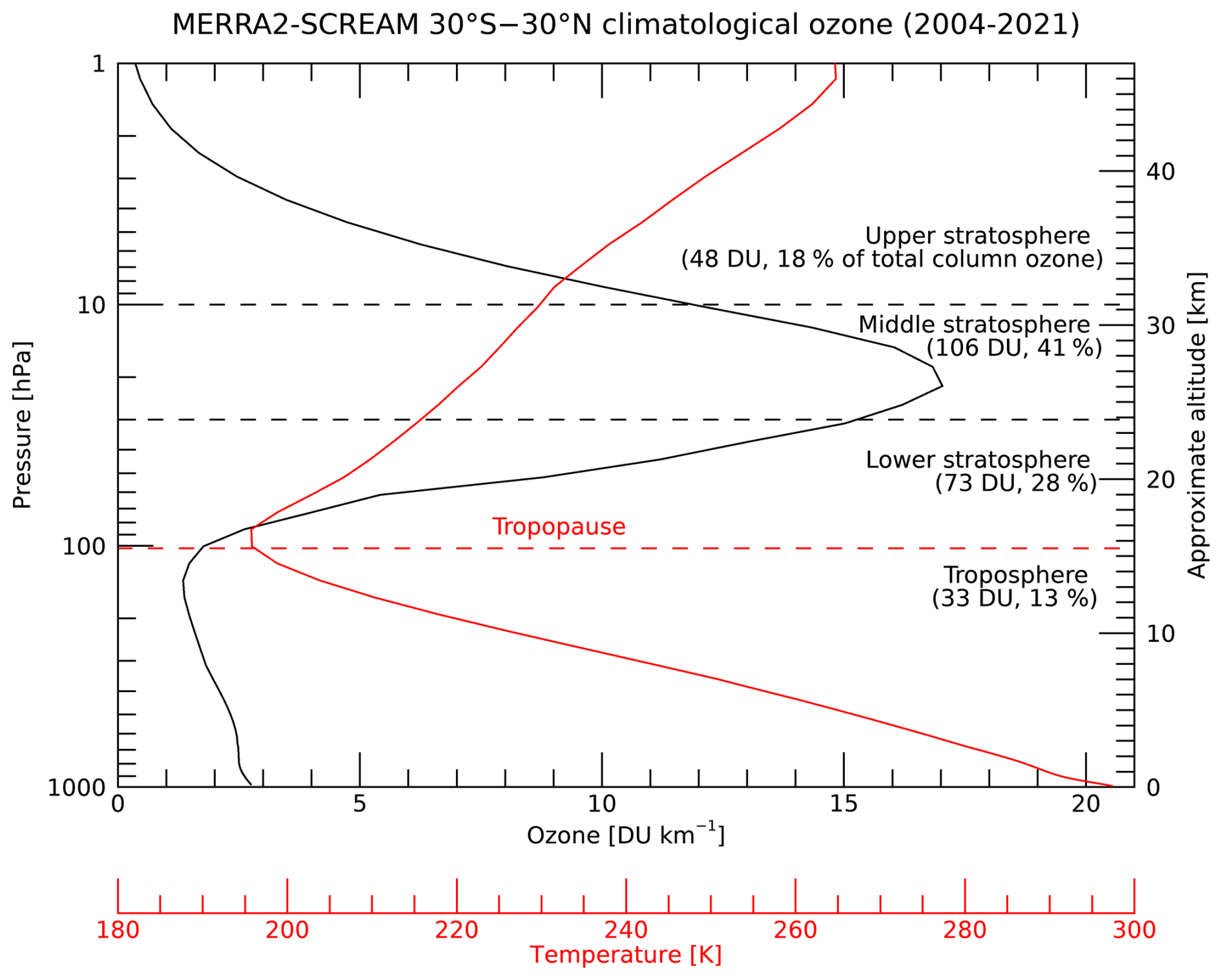
Figure 1 The 2004–2021 climatological tropical average (30° S–30° N) ozone profile from MERRA-2 Stratospheric Composition Reanalysis of Aura MLS (MERRA2-SCREAM, black), along with the corresponding temperature profile (red). The relative contributions to total column ozone from each of the four vertical layers considered in this paper are given on the right hand side.

The first sections (Sects. 2–4) of the paper detail the observational datasets, CCMs, and statistical methods used. Then, in section 5 we intercompare the recent ozone changes simulated by CCMs and derived from observations to illustrate regions of agreement and disagreement. Next (Sect. 6), we analyze the long-term ozone changes and demonstrate that in the models, data from the first ∼ 2 decade period of ozone recovery is sufficient to separate the slowly-varying “recovery” signal from natural variability, and (Sect. 7) that the models' recovery signal over this period is predictive of the end-of-the-century behavior. While this emergent behavior in the models lends itself in principle to an observational constraint on the credibility of modeled future tropical ozone for a given scenario, we demonstrate in Sect. 8 that current range of observational trend estimates is too large to effectively serve as an observational constraint.

Table 1 Observational datasets.

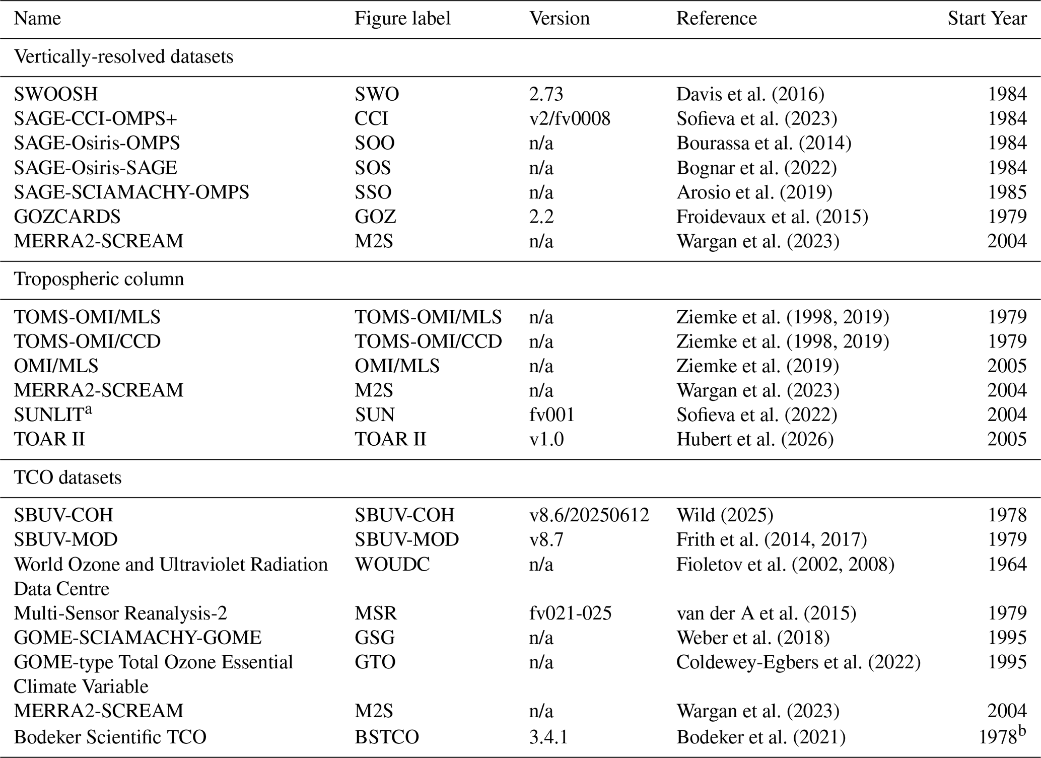
^a Dataset also includes stratospheric column ozone. ^b Dataset ends in 2019.
n/a: not applicable.

2 Ozone observations and reanalyses

This section describes the satellite observational and reanalysis datasets that are used for estimating historical ozone changes. The datasets include vertically-resolved stratospheric data, from which we compute partial column ozone timeseries across various layers of the stratosphere, as well as total/partial column datasets that provide pre-computed values. The datasets described herein are summarized in Table 1.

2.1 Vertically-resolved datasets

We briefly describe here several merged datasets based on vertically-resolved ozone retrievals from satellite instruments operating in solar occultation and limb-viewing geometries. These datasets are provided as monthly zonal means with horizontal grid spacings from 2.5 to 10° in latitude. We note that in general many of these datasets rely on overlapping subsets of instruments, and so are not entirely independent. Of particular note, all of the merged datasets here include data from the Stratospheric Aerosol and Gas Experiment II (SAGE II) instrument (1984–2005), and as such many of the datasets start part way through 1984 with the beginning of the SAGE II record. Also, a number of datasets are subject to large changes in tropical sampling (e.g., with the inclusion of the Aura Microwave Limb Sounder (MLS) in 2004 or the Ozone Profiler and Mapping Suite Limb Profiler (OMPS-LP) in 2012), and these sampling changes have potential impacts on the ability to constrain ozone trends. As an example, whereas the solar occultation instruments collect ∼ 30 vertical ozone profiles per day and may go entire months without sampling the tropics (depending on orbit), the median tropical sampling for Aura MLS and OMPS-LP is 1200 and 800 profiles per day, respectively (Hegglin and Tegtmeier, 2017).

Two of the merged datasets used here rely heavily on Aura MLS measurements. The first of these is the Stratospheric Water and OzOne Satellite Homogenized (SWOOSH) dataset (Davis et al., 2016) version 2.73, whose merged ozone product includes data from SAGE II (v7), the Upper Atmosphere Research Satellite Halogen Occultation Experiment (UARS HALOE v19), UARS MLS (v5), SAGE III/Meteor (v4), Aura MLS (v5.0), Atmospheric Chemistry Experiment Fourier Transform Spectrometer (ACE-FTS, v5.2), and SAGE III/ISS (v5.3). In SWOOSH, the merged product in a given latitude-pressure-month bin is the mean of all available monthly means from each source instrument operating in that month, weighted by the number of profiles for the given instrument. Because of this weighting, instruments with dense sampling such as Aura MLS dominate the merged product.

The other Aura MLS-based merged dataset considered here is the Global OZone Chemistry And Related trace gas Data records for the Stratosphere v2.2 (GOZCARDS, Froidevaux et al. 2015). GOZCARDS includes SAGE I (v5.9, 1979–1981), SAGE II (v7), and Aura MLS (v4.2). Although SWOOSH and GOZCARDS are similar, the two datasets use a slightly different approach for homogenization during instrument overlap periods, and GOZCARDS weights each source instrument equally in the combined product, unlike SWOOSH, which weights based on the number of profiles. In practice, the different weightings are most likely to cause differences between the products prior to the end of 2005, when the HALOE and SAGE II records terminated.

In addition to the Aura MLS-based datasets, we include in our analysis several datasets that rely on different combinations of instruments in the 2000's. First is the SAGE-CCI-OMPS+ (CCI) dataset (v2/fv0008, Sofieva et al., 2023), which combines data from SAGE II (v. 7), three instruments (GOMOS ALGOM2s v.1, MIPAS KIT v8, SCIAMACHY UBr v3.5) aboard the Environmental Satellite (Envisat, 2002–2012), Optical Spectrograph and InfraRed Imaging System (OSIRIS, v7.2, beginning 2002), ACE-FTS, and two retrievals of SNPP OMPS-LP data (UBr v3.5, Arosio et al., 2018; USask2D v1.1.0, Zawada et al., 2018). Deseasonalized anomalies of the source records are used to construct the merged data product, and as such the weighting of individual source records in the merged product is similar to GOZCARDS. We also use two OSIRIS-centered products, the SAGE-OSIRIS-OMPS (SOO, Bourassa et al., 2014, 2018; Zawada et al., 2018) and SAGE-OSIRIS-SAGE (SOS, Bognar et al., 2022) datasets. SOO consists of SAGE II (v7.0), OSIRIS (v7.3), and SNPP OMPS-LP (USask v1.3), while SOS does not use OMPS-LP and instead uses SAGE III/ISS (v5.3), whose record begins in 2017. The SOO and SOS composites use a similar merging methodology as the CCI dataset, based on merging monthly mean deseasonalized anomalies. Given the overlap in instruments, these two datasets should be virtually identical prior to the introduction of SNPP OMPS-LP in 2012. In addition to the OSIRIS-centered products, we also use the SAGE-SCIAMACHY-OMPS (SSO, Arosio et al., 2019) dataset. SSO consists of SAGE II (v7.0), SCIAMACHY (v3.5), and OMPS-LP (UBr v4.1). The merging of these time series is also based on deseasonalized anomalies, and Aura MLS is used as a transfer function between SCIAMACHY and OMPS-LP due to the short overlap between the latter two.

Finally, we also include ozone from the MERRA-2 Stratospheric Composition Reanalysis of Aura MLS (M2-SCREAM, Wargan et al., 2023), which covers the same period as Aura MLS (September 2004 to December 2024). M2-SCREAM assimilates stratospheric ozone, water vapor, hydrogen chloride (HCl), nitric acid (HNO₃) and nitrous oxide (N₂O) from Aura MLS (v4.2 before 2024, v5.0 thereafter) as well as Aura Ozone Monitoring Instrument (OMI) TCO between 2004 and 2024. Because both OMI TCO and vertically-resolved stratospheric MLS data are assimilated by M2-SCREAM, it is likely that some constraint exists on tropospheric ozone amounts, although it should be stressed that the M2-SCREAM chemical scheme does not include tropospheric ozone chemistry reactions. Thus, while M2-SCREAM is not an entirely independent dataset, it serves as a useful way to verify consistency among the various MLS-based datasets.

2.2 Total column ozone data

We use a number of monthly mean total column ozone datasets here, most of which are based on merged satellite-based records. Except where otherwise noted, these datasets are the same as those used by Weber et al. (2022), and the reader is referred there for a more complete overview. Briefly, we use the SBUV-COH (v8.6/20250612, Petropavlovskikh et al., 2025; Wild, 2025) and SBUV-MOD (v8.7, Frith et al., 2014, 2017) merged datasets based on the Backscatter Ultraviolet (BUV), Solar Backscatter Ultraviolet (SBUV), and OMPS Nadir Profiler (NP) instruments operated from aboard NOAA satellites since the late 1970's. These datasets merge data from the same set of instruments but with different choices regarding the use of individual satellites, homogenization and orbital drift/diurnal corrections.

We also use two merged datasets based on the Global Ozone Monitoring Experiment (GOME) instruments, the GOME-SCIAMACHY-GOME (GSG) dataset (Weber et al., 2018) and the GOME-type Total Ozone Essential Climate Variable (GTO-ECV, hereinafter GTO; Coldewey-Egbers et al., 2022) data record, both based on GOME and GOME-2 instruments plus several other sensors (SCIAMACHY, OMI, and TROPOMI). In addition to using different sets of instruments, the two GOME-based datasets use different algorithms for retrieving TCO, as well as different homogenization methods.

We also use data from the gap-filled Bodeker Scientific TCO dataset (BSTCO v3.4.1, Bodeker et al., 2021). This dataset includes data from 17 different satellite instruments operating since the late 1970's, including multiple SBUV, GOME, and TOMS instruments, as well as SCIAMACHY, OMI, and OMPS Nadir Mapper. Note that this dataset was not used by Weber et al. (2022).

In addition to the merged satellite data records, we also use monthly mean zonal mean ground-based Dobson and Brewer data from the World Ozone and Ultraviolet Radiation Data Centre (WOUDC) dataset (Fioletov et al., 2002, 2008).

Finally, we also use TCO data from two assimilated products that were not considered by Weber et al. (2022): the Multi-Sensor Reanalysis-2 (MSR-2, hereinafter MSR; van der A et al., 2015) and M2-SCREAM. MSR bias-corrects all available TCO data from polar-orbiting satellites based on ground-based Brewer/Dobson instruments from WOUDC, and then assimilates the debiased observations using the Tracer Model Data Assimilation Model (TMDAM) ozone chemistry and data assimilation model driven by ECMWF analysis fields.

2.3 Tropospheric column data

We consider tropospheric partial column ozone (TrCO) from several datasets here. These satellite-based datasets use a “residual” technique whereby the measured or integrated (e.g., from a retrieved ozone profile) stratospheric partial column ozone value is subtracted from a TCO observation.

One residual tropospheric column dataset comes from Aura OMI and Aura MLS (hereinafter OMI/MLS, Ziemke et al., 2019), which uses the OMI TCO and the stratospheric column from the Aura MLS v4.2 data above the WMO lapse rate tropopause provided by the National Centers for Environmental Prediction (NCEP) reanalysis.

Another residual dataset is provided by the Synergy of Using Nadir and Limb Instruments for Tropospheric Ozone Monitoring (SUNLIT) project (Sofieva et al., 2022). SUNLIT covers 2004 to present using OMI and TROPOMI TCO, combined with a separate stratospheric column dataset consisting of Aura MLS, OSIRIS, Michelson Interferometer for Passive Atmospheric Sounding (MIPAS), SCanning Imaging Spectrometer for Atmospheric CHartographY (SCIAMACHY), S-NPP OMPS-LP, and Global Ozone Monitoring by Occultation of Stars (GOMOS).

Two additional TrCO datasets come from the Total Ozone Mapping Spectrometer convective-cloud differential approach (TOMS CCD; Ziemke et al., 1998, 2019) which uses ozone columns retrieved above deep convective clouds as a proxy for the stratospheric column, and subtracts these values from the total column retrieved from clear-sky scenes. This CCD technique is also applied to OMI data to form a TOMS + OMI CCD dataset from 1979 to present. Additionally, we also consider a merged dataset consisting of TOMS CCD before Oct 2004, and OMI/MLS after (hereinafter TOMS+OMI/MLS).

In addition to the satellite merged data sets, we also use TrCO from M2-SCREAM. As M2-SCREAM assimilates MLS ozone in the stratosphere and OMI TCO, it is not expected that this product would be substantially different from the OMI/MLS dataset. However, M2-SCREAM also assimilates other ozone-relevant stratospheric species from MLS and represents meteorological variables that could impact ozone, both in the troposphere and stratosphere, so it is not expected to be identical to the OMI/MLS dataset.

Finally, we consider a multi-dataset merged product produced by the TOAR II activity (Hubert et al., 2026). This TOAR II dataset consists of 15 satellite TrCO data records spanning nadir profiling, tropospheric ozone residual (e.g., like OMI/MLS), and convective-cloud differential techniques. We note that the datasets contributing to the TOAR II multi-dataset product include the OMI/MLS and SUNLIT datasets also analyzed separately in this paper.

2.4 Stratospheric column data

Ozone from the vertically-resolved satellite datasets (SWOOSH, GOZCARDS, SOO, SOS, CCI) and M2-SCREAM is vertically integrated to obtain partial ozone columns in the stratosphere. The whole-stratosphere PCO is computed by integrating from the MERRA-2 zonal mean tropopause to 1 hPa (or 48 km for the altitude-gridded datasets). Prior to this integration, we infill any missing ozone data values by interpolating merged ozone anomalies in the latitude-height plane, as in Davis et al. (2016). In addition to the integration over the entire stratosphere, we also consider PCO in layers covering the lower stratosphere (tropopause to 30 hPa/24 km), middle stratosphere (30 to 10 hPa/31 km) and upper stratosphere (10 to 1 hPa/48 km), as illustrated in Fig. 1.

In addition to the vertically-resolved datasets that we integrate to get stratospheric PCO, we also consider the stratospheric column data produced as part of the SUNLIT dataset (Sofieva et al., 2022). The SUNLIT stratospheric column represents a vertical integration over the stratosphere from a combination of limb instruments including OSIRIS, GOMOS, SCIAMACHY, MIPAS, OMPS-LP, and Aura MLS.

3 Chemistry Climate Models

An overview of the Chemistry-Climate Models (CCMs) used in this study is provided in Table 2. Phase 1 of the Chemistry-Climate Model Initiative (CCMI-1) involved a set of coordinated simulations from a set of 20 CCMs and Chemistry-Transport Models (CTMs) that explicitly represent atmospheric chemistry and are suitable for studying a variety of processes including both stratospheric and tropospheric chemistry, as well as global climate change (Morgenstern et al., 2017). Models participating in CCMI-1 were generally of the same generation as the 5th Coupled Model Intercomparison Project (CMIP5) and used forcings similar to that activity, but the reader is referred to Morgenstern et al. (2017) for further details on individual models. A variety of simulations covering the middle 20th century through the end of the 21st century were performed as part of CCMI-1, but only the relevant experiments are briefly described here. The REF-C2 simulations cover 1960 through 2100 using ozone depleting substance (ODS) concentrations from the WMO 2010 Scientific Assessment of Ozone Depletion (SAOD) A1 scenario (WMO, 2011), and other forcings including aerosols, greenhouse gases, and tropospheric ozone precursors from Representative Concentration Pathway (RCP) 6.0 (Meinshausen et al., 2011). In REF-C2 simulations, the ocean state is either coupled to the atmosphere model or prescribed based on an offline ocean simulation. A comprehensive description of the REF-C2 experimental design is provided by Eyring et al. (2013). Additionally, we include analysis of the fixedGHG scenario, which is identical to REF-C2 except with GHGs fixed at 1960 values to isolate the impacts of ODSs separately.

In addition to CCMI-1 model output, we also consider simulations performed as part of the follow-up CCMI-2022 project (Plummer et al., 2021). We use the CCMI-2022 future projection simulations (REF-D2, 1960 to 2100), which are a similar configuration to the older CCMI-1 REF-C2 simulations. CCMI-2022 model generations and forcings are generally similar to those from CMIP6. For REF-D2, greenhouse gas and anthropogenic precursor forcings are from the CMIP6 historical database (Meinshausen et al., 2017) up to 2014 and SSP2-4.5 thereafter (Meinshausen et al., 2020; O'Neill et al., 2016). Near-surface ODS mixing ratios are specified based on the WMO (2018) baseline scenario. In comparison to the WMO 2010 scenario, the WMO 2018 scenario has a virtually identical peak value of equivalent effective stratospheric chlorine (EESC), but a slower decline that results in a 5 year delay in the return date to 1980 values (Lickley et al., 2024). A comprehensive description of the CCMI-2022 simulations is provided by Plummer et al. (2021).

Table 2 Chemistry climate models used in this study to simulate ozone from 1960 to 2100.

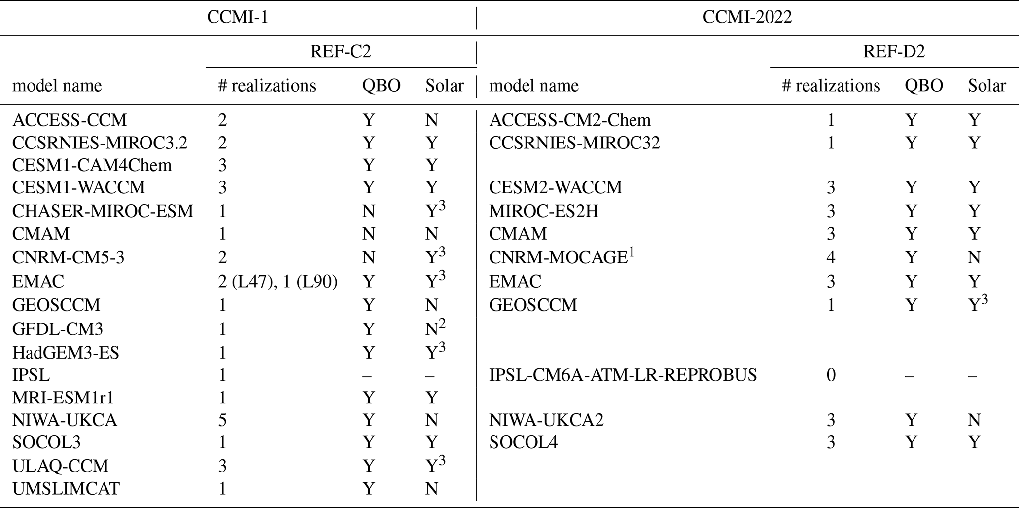
¹ Tropospheric ozone not included in analysis, due to unphysical jumps. ² Solar variability in radiative scheme, but not implemented in photolysis code. ³ Non-standard solar forcing used.

For REF-C2 simulations, most of the participating models used nudging of their equatorial winds to represent the QBO (Table 2, see also Table S8, Morgenstern et al., 2017), and the other models either had no QBO at all or an internally generated one. For the former, a forcing dataset was provided based on observed equatorial winds through 2011 that then repeats past cycles into the future. As this is not explicitly documented, we report based on visual inspection (not shown), that seven REF-C2 models are nudged towards this forcing dataset, four models have no apparent QBO wind variability, and the rest exhibit QBO variability in their winds that is not synchronized with observations in the pre-2012 period.

Overall, the QBO representation in models improved from the CMIP5-class models used in CCMI-1 to the CMIP6 models used in CCMI-2022 (Richter et al., 2020), and the specification of QBO treatment in REF-D2 resulted in a more consistent treatment across models. In REF-D2, models containing an internally generated QBO were allowed to generate their own QBO, whereas models that do not were directed to nudge towards an extended QBO dataset. In contrast to REF-C2, all REF-D2 models exhibit QBO-like variability in their equatorial stratospheric winds, and only three models appear to have nudged their wind fields towards historical observations.

4 Dynamical linear modeling

Dynamical linear modeling (DLM) is a statistical method for time series modeling that is functionally similar to multiple linear regression (MLR), but with several important differences, most notably the use of a flexible non-parametric background term for capturing “trends”, as well as principled treatment of auto-regressive processes and time-varying uncertainties (Laine et al., 2014). The DLM technique has been used in a number of recent studies to quantify ozone depletion and recovery trends (Ball et al., 2017, 2018, 2019; Bognar et al., 2022; Davis et al., 2023; Maillard Barras et al., 2022; Van Malderen et al., 2025).

In this study, we use the dlm_vanilla_ar1 model from the dlmmc software package (Alsing, 2019) with its default hyperparameter settings. This model includes dynamic seasonal cycles (2 cos/sin harmonic pairs) and background trend, fixed (non-dynamic) proxy terms (described in the next section), as well as a first-order autoregressive process (AR1). We run the DLM for each observational and model dataset, and for each atmospheric layer described above, using monthly mean tropical-averaged (30° S–30° N) PCO/TCO. From the DLM, we infer ozone changes by sampling the posterior distribution of the background trend term from simulations with 7000 iterations (2000 of which are used as warmup and discarded), and report either the percentage of posterior changes of a given sign (e.g., 95 %) or the standard deviation of the posterior distribution as measures of trend significance and uncertainty, respectively. In some cases, we also show kernel density estimates (KDEs) of changes in the DLM background ozone values. KDEs are a non-parametric method used to estimate the probability density function (PDF) of a variable by applying a smoothing kernel, and by construction are normalized to unity. For each observational dataset, KDEs are computed from the 5000 iterations of the DLM model. Multi-model KDEs are constructed by sampling 5000 DLM iterations across all available realizations of each CCM participating in the given multi-model experiment. For models with only one realization, all 5000 iterations of the DLM are used. Similarly, we construct the multi-observational KDE by sampling across the 5000 DLM iterations available from each observational data set. We note that the choice of 7000 iterations is likely far more than necessary, but represents a balance between sample size, reasonable computing time, and stability of the hyperparameters. Our testing has indicated virtually identical results for an order of magnitude fewer iterations.

As with other studies, for the DLM simulations on CCM output we do not input uncertainty values to the DLM model. When running the DLM on the observational composites, we use a 1 % uncertainty. While this number may seem small given typical reported precision uncertainties of ∼ 10 % from satellite limb instrument ozone retrievals, we note that these random errors are substantially reduced by both vertical averaging and the averaging of the many profiles within the tropics for a given month. The 1 % number used here is a reasonable choice based on testing we did (not shown) with the SWOOSH data using propagation-of-errors including covariance estimates (i.e., not assuming independent measurements), and is also justified based on the clear geophysical variability present in the PCO/TCO timeseries that is on the order of 1 % (see, e.g., example in Sect. 4.2). We note that, while the DLM posterior uncertainties are influenced by data uncertainties input to the DLM, the output uncertainties are non-zero even for zero input uncertainty, and are not strongly sensitive to the input uncertainties (e.g., doubling the input uncertainty from 1 % to 2 % does not double the posterior uncertainty).

4.1 Regressor proxies

Here we briefly describe the regressor proxies used in the DLM runs of PCO from models and observations. As our goal is to isolate the slowly-varying background ozone trend term consistently from models and observations, we use proxies that are appropriate for each dataset.

For applying to observations, we use as proxies the detrended Oceanic Niño 3.4 Index from the NOAA Climate Prediction Center to represent the El Niño Southern Oscillation (ENSO), the first two principal components (PCs) from the MERRA-2 reanalysis equatorial stratospheric (100–10 hPa) winds to represent the QBO, the 30 cm radio flux to represent the 11-year solar cycle, and the tropical (30° S–30° N) stratospheric aerosol optical depth (SAOD) from the most recent (v2.21) GloSSAC dataset (Kovilakam et al., 2020).

For models, we compute the ENSO index by averaging and detrending the surface temperatures from each simulation over the Niño 3.4 region (170–120° W, 5° S–5° N). For representing the QBO we use the first two PC timeseries computed for each model using the same methodology described above for MERRA-2.

For representing the solar cycle in REF-D2, we use the recommended CMIP6 solar forcing as described by the SOLARIS-HEPPA working group (https://solarisheppa.geomar.de/cmip6, last access: 20 May 2024). We identify which models represent solar ozone variability (see Table 2) by identifying those with a significant correlation between the recommended solar forcing timeseries and a smoothed version of the tropical upper stratospheric partial ozone column (i.e., the residual after fitting using the dlm_noregs_ar1 model), similar to the approach taken by Funke and Matthes (2020, see their Fig. 19). We find that in REF-D2, models either used the recommended solar forcing or don't exhibit solar cycle ozone variability.

In contrast, using the same type of analysis with REF-C2 output, we find that a number of models, while including solar cycle variability, did not implement the recommended forcing (Table 2; forcing details at https://solarisheppa.geomar.de/ccmi, last access: 20 May 2024). While all models used a solar forcing consistent with observations prior to 2011, after this time many of the models repeated a different solar cycle (or set of solar cycles) than the recommendation, which was to repeat a sequence of the last four solar cycles (20–23). As a result, the correlation coefficients between the recommended forcing and residual ozone are much smaller after 2011 in some models, as the phasing between the two drifts apart. For these models, we used the appropriate solar forcing provided by the modeling groups directly, or in one case (CHASER-MIROC-ESM) inferred the solar input based on mesospheric O¹D photolysis rate output at 0.1 hPa.

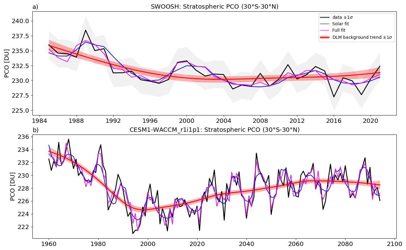
Figure 2 Example DLM fits to the annual and tropical (30° S–30° N) mean partial column ozone (PCO) time series for the whole stratosphere (tropopause to 1 hPa, black lines) from (a) the SWOOSH observational dataset (with ±1σ uncertainty shading in gray) and (b) a CESM1-WACCM simulation from REF-C2. Shown are the DLM background trend terms (red line is the mean trend with ±1σ uncertainty shading), which are the primary focus of the analysis presented here. Also shown are the 11-year solar cycle component of the fit (blue) along with the full DLM fit (i.e., trend + all proxies including QBO, ENSO, Solar, and SAOD).

4.2 DLM example

To illustrate the DLM fitting process and give a qualitative sense of what the DLM fits look like, Fig. 2 shows an example fit to one observational dataset (SWOOSH) and one REF-C2 model (CESM1-WACCM) for the tropical stratospheric PCO. Although DLM fits are performed on monthly data, the figure shows annual mean data to better illustrate interannual variability, such as that due to ENSO, QBO, and solar cycle variability. This figure highlights the large interannual variability over the SWOOSH observational period in comparison to the relatively small DLM background trend changes (Fig. 2a), which ultimately contribute to the uncertainties in the inferred background change. The solar component of the fits demonstrates the prominent 11-year solar cycle in both timeseries to illustrate why it is important to include this regressor, in particular when attempting to extract a background trend over shorter time periods such as the SWOOSH observational record.

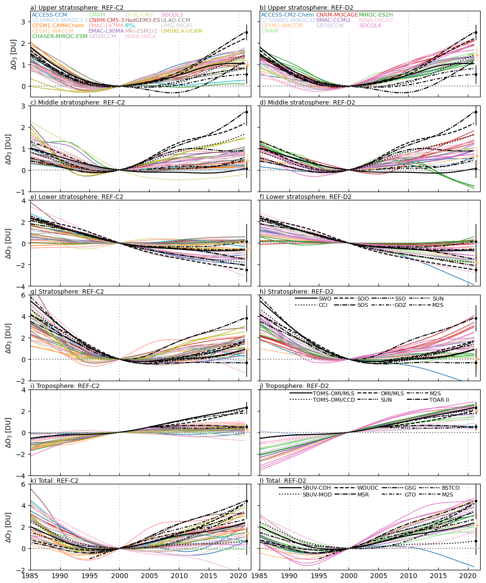
Figure 3 DLM background trend timeseries over the “observational period” (1985–2021) for REF-C2 simulations (colors, left column), REF-D2 (colors, right column) and observations (black) relative to 2000 for (a) the upper stratospheric PCO, (b) middle stratospheric PCO, (c) lower stratospheric PCO, (d) whole stratospheric PCO, (e) tropospheric PCO, and (f) the TCO. At the end of the timeseries, a few selected examples are shown of the DLM background trend ozone change over 2000–2021, with error bars denoting ± 1 standard deviation of the DLM changes (see text for discussion). For tropospheric PCO datasets starting in 2005 (i.e., SUNLIT, OMI/MLS, and M2S), the timeseries have been adjusted to match the TOMS-OMI/MLS value in 2005 for easy comparison across datasets, and the changes have been scaled to represent the equivalent change over 2000–2021. Note, CNRM-MOCAGE data are excluded from panels (j) and (l) due to an unphysical jump in tropospheric ozone near the end of simulation. To facilitate easy comparison, the y-axes span 8 DU for all layers except for the middle and upper stratosphere, which span 4 DU.

5 Tropical ozone changes: satellite observational period

In this section, we consider tropical ozone changes over the observational time period, starting in 1979 for total column and tropospheric partial column data, and 1985 for stratospheric partial column data. These choices coincide with the first full year of the available datasets, which are constrained by the starting dates of the TOMS (November 1978) and SAGE II datasets (October 1984). For the end date, we use 2021, as it occurs prior to the eruption of the Hunga volcano, which was shown to have impacted stratospheric composition following the eruption, with potential implications for ozone (APARC, 2025; Santee et al., 2023). Any ozone impacts from this eruption (e.g., from stratospheric aerosol and water vapor perturbations) are not included in either of the REF-C2 or REF-D2 simulations, but are potentially present in the observational datasets.

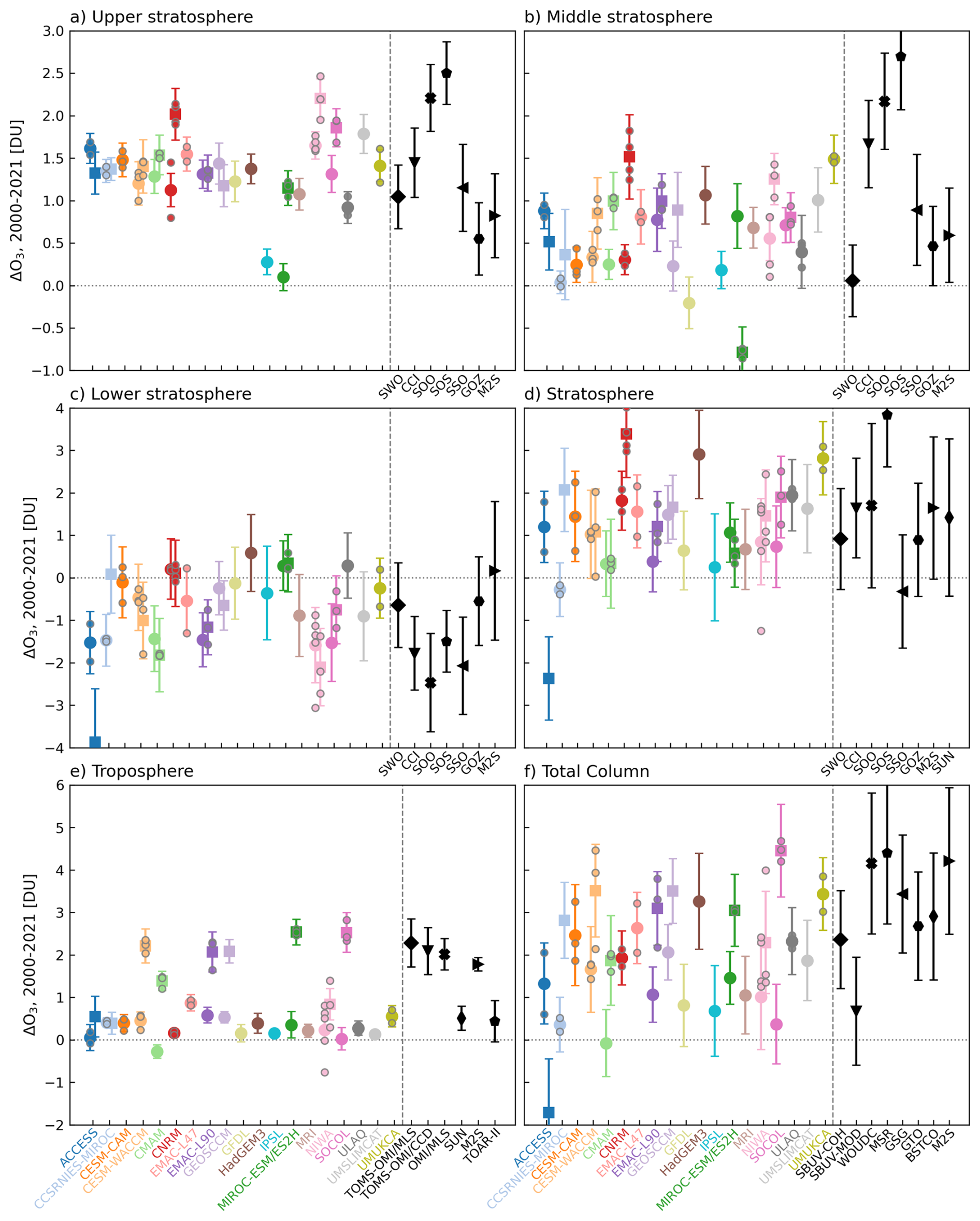
Figure 4 DLM background trends over the early recovery period (2000–2021) for each model from REF-C2 simulations (circles), REF-D2 simulations (squares), and observations (black) for (a) the upper stratospheric PCO, (b) middle stratospheric PCO, (c) lower stratospheric PCO, (d) whole stratospheric PCO, (e) tropospheric PCO, and (f) the TCO. To facilitate easy comparison, the y-axes span 8 DU for all layers except for the middle and upper stratosphere, which span 4 DU.

Figure 3 shows the DLM background trend term from the fit to the tropical average (30° S–30° N) PCO in three stratospheric layers, the whole stratosphere, and troposphere, as well as TCO from both the observations and model simulations. A trend summary derived from this figure is shown in Fig. 4. All DLM changes are shown relative to the year 2000 to allow for easy comparison between changes since that time.

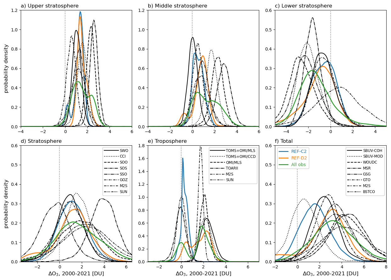
Figure 5 Kernel density estimates (KDEs) of DLM background trend change (2000–2021) in tropical ozone columns from observations (black lines for individual data sets, green lines for the multi-observational distributions), REF-C2 (blue), and REF-D2 (orange). Results from observational datasets starting in 2005 (i.e., OMI/MLS, SUNLIT, M2S) have been scaled to represent changes over the 2000–2021 period instead of the 2005–2021 period.

To complement these figures, Fig. 5 shows kernel density estimates (KDEs) of changes in the DLM background ozone trend since 2000, from both multi-model experiments and observations. To quantify the degree of agreement between the trend estimates, we compute the overlap coefficients between pairs of trend distributions (Inman and Bradley, 1989). The overlap coefficient is defined as the area intersected by two probability density functions, and is computed here by numerically integrating the minimum of the two KDEs. The overlap of the two KDEs is then expressed as a percentage, with 0 % indicating distributions with no overlap and 100 % indicating identical distributions. Overlap coefficients are discussed below in the context of specific comparisons between models and observations. A comprehensive set of overlap coefficients for all combinations of models, observations, and atmospheric layers are provided in the Supplement (Figs. S1–S6), alongside a table of the mean DLM changes (Table S1).

Together, these figures demonstrate a varied level of agreement amongst the models, amongst the observations, and between models and observations across the different vertical layers of the atmosphere. Below, we summarize some of the key the similarities and differences between the models and observations, and highlight the notable differences between the REF-C2 and REF-D2 experiments.

5.1 Upper stratosphere

In the upper stratosphere (10–1 hPa), the spread of CCM responses is fairly narrow and there is a large degree of overlap between REF-C2 (+1.2 DU over the 2000–2021 period, Fig. 5a) and REF-D2 experiments (+1.5 DU). However, there is a wide spread amongst the observational datasets since 2000, with some datasets showing quite strong recovery values that are generally above the spread of REF-C2 models (SOS, mean $=+\mathrm{2.6}$ DU; SOO, mean $=+\mathrm{2.3}$ DU), some near the middle of the model spread (M2-SCREAM, mean $=+\mathrm{1.2}$ DU; SSO, mean $=+\mathrm{1.2}$ DU; CCI, mean $=+\mathrm{1.5}$ DU), and the MLS-based datasets on the lower end (SWOOSH, mean $=+\mathrm{1.0}$ DU; GOZCARDS, mean $=+\mathrm{0.6}$ DU).

For the tropical upper stratosphere changes over 2000–2021, the observational datasets with the least (GOZCARDS, mean change of +0.55 DU) and most (SOS, mean change of +2.6 DU) upper stratospheric ozone increase have very little overlap with one another (2 %). In the middle lies the CCI dataset, which overlaps somewhat with each of these observational datasets (28 % for GOZCARDS and 21 % for SOS). In contrast to the spread amongst observational estimates, the REF-C2 and REF-D2 upper stratospheric changes since 2000 are in good agreement with one another, showing an increase of 1.3 and 1.5 DU, respectively, with an overlap of 85 %. Although there is a large spread of observational estimates, the CCI data shows good agreement with the models (75 % and 79 % overlap for REF-C2 and REF-D2, respectively), as does M2-SCREAM although to a lesser extent (67 % and 59 % overlap).

5.2 Middle stratosphere

In the middle stratosphere (30–10 hPa), the model experiments are also in good agreement, with REF-C2 (REF-D2) showing an increase of 0.7 DU (0.5 DU) since 2000 (81 % overlap). Similarly to the upper stratosphere, the observations show a wide range, with SWOOSH showing a small positive change (mean of +0.1 DU), SOS showing a strongly positive change (mean increase of 2.5 DU), and a negligible 2 % overlap between the two. Even neglecting these two outlier datasets, the range of observational estimates in the middle stratosphere is large. For example, the next most negative dataset (GOZCARDS) has a +0.5 DU increase, whereas the next most positive dataset (SOO) contains a +2.3 DU increase, with only 10 % overlap between the two. As for the agreement between models and observations, in this region both M2-SCREAM and GOZCARDS have the best overlap with the models (78 %/79 % between REF-C2/REF-D2 and M2-SCREAM; 86 %/72 % for GOZCARDS).

Given that GOZCARDS, M2-SCREAM, and SWOOSH are all primarily reflecting Aura MLS data after 2004, it is somewhat surprising that they give different results. A sensitivity analysis where the DLM was provided SWOOSH and GOZCARDS data starting in 2005 shows nearly identical 2005–2021 changes between the two datasets (95 % overlap), in contrast to changes over the same time period (2005–2021) but with DLM input data starting in 1985 as in Fig. 5 (71 % overlap). Also using 2005–2021 data as input to the DLM, we find that SWOOSH and GOZCARDS show good agreement with M2-SCREAM (75 % and 78 % overlap, respectively). Together, these results indicate that trend differences in Fig. 5b over 2000–2021 are not a result of using different versions of Aura MLS data (SWOOSH uses v5, whereas GOZCARDS and M2-SCREAM use v4.2). An additional test using DLM input data starting in 2000 produces a 78 % overlap between SWOOSH and GOZCARDS for 2000–2021 changes, as compared to the 63 % overlap in Fig. 5b (based on input data starting in 1985). This suggests that the trend differences between SWOOSH and GOZCARDS in Fig. 5b are due to both underlying data differences during the 2000–2004 pre-Aura MLS time period, as well as to differences in pre-2000 data impacting the background trend value in the year 2000. As SWOOSH and GOZCARDS use the same satellite data and data versions in the pre-Aura period, the exact cause of these differences is presumably due to different processing/filtering of the input profiles or merging methodology, and will be the subject of future investigation.

5.3 Lower stratosphere

In the lower stratosphere (tropopause to 30 hPa), the CCMs show negative mean changes over 2000–2021 (−0.6 DU for REF-C2 and −1.1 DU for REF-D2) and significant overlap between the two distributions (88 %). The CCM distributions are 69 % and 77 % negative for REF-C2 and REF-D2, respectively. All of the observations except for M2-SCREAM (+0.7 DU) show negative mean changes over this time period, with values ranging from −2.6 (SOO) to −0.6 DU (GOZCARDS). Although the models and observations mostly show robust negative changes, we note that the percentage of posteriors with negative values ranges from insignificant (71 % for GOZCARDS) to highly significant (>95 % for SSO, SOO, SOS, and CCI). Finally, as with the other regions of the stratosphere, in the lower stratosphere the degree of overlap between the observations and models varies widely, from about 40 % (SOO and REF-C2) to 95 % (GOZCARDS and REF-C2).

5.4 Whole stratosphere

Considering the stratosphere as a whole, both observational estimates and CCMs predominately show increases over the 2000–2021 time period. As with the other regions of the stratosphere, the CCM ensembles show a large degree of overlap (90 %), even though their mean increases are somewhat different (1.4 DU for REF-C2 vs. 1.0 DU for REF-D2). It is worth noting that the ACCESS-CM2-Chem is an outlier in the stratospheric column timeseries (Fig. 4d). Excluding this model, the mean REF-D2 change is +1.5 DU, and the two distributions have 98 % overlap. Observations also span a wide range, varying from −0.4 DU for SSO to +3.9 DU for SOS with 11 % overlap between the two. The observational estimates closest to the CCM means (i.e., GOZ, +0.9 DU; SOO, +1.7 DU) show quite strong overlap with one another (72 %). The overlap between CCMs and observations ranges from ∼ 30 %–50 % for the SOS and SSO datasets, respectively, to ∼ 70 %–90 % for the other observational datasets (Fig. S4).

5.5 Troposphere

In the troposphere, there are stark differences between the observational datasets and also between the two CCM experiments. For example, REF-C2 shows a relatively small change in tropical tropospheric ozone over the 2000–2021 period (+0.4 DU), whereas the overall REF-D2 distribution shows substantial increases (+1.4 DU). With only 40 % overlap between the two CCM distributions, the troposphere is the region of greatest (and arguably, only substantial) difference between the two modeling experiments. Although we do not attempt to quantitatively attribute the differences in tropospheric ozone changes between REF-C2 and REF-D2, we do note that the tropospheric precursor emissions are very different between the two experiments, and that this seems to be the most likely contributor to differences among the datasets (Acquah et al., 2025). For example, from 2000 to 2020 the REF-C2 tropical-average NO_x emissions increased from ∼ 30 to ∼ 40 Tg yr⁻¹, whereas in REF-D2 the emissions rose from ∼ 50 to ∼ 70 Tg yr⁻¹, almost a factor of two greater increase. Our analysis cannot rule out, however, that the differences in tropical tropospheric ozone evolution between REF-C2 and REF-D2 also have a contribution due to changes in the complexity of tropospheric ozone chemistry in the newer generation of models, with a larger proportion of the earlier REF-C2 models (e.g. UMUKCA-UCAM, HadGEM3-ES, CMAM) using chemistry schemes tailored primarily for stratospheric ozone studies while employing a reduced-complexity approach to tropospheric chemistry.

Similarly large discrepancies exist between the observational estimates of tropospheric change. For example, the SUNLIT dataset shows a 0.0 DU mean change, whereas the TOMS+OMI/MLS dataset shows an increase of 2.4 DU (with 1 % overlap between the two). We note that the SUNLIT dataset shows strong overlap with the REF-C2 distribution (64 %), whereas the TOMS+OMI/MLS dataset overlaps strongly with the REF-D2 distribution (65 %).

5.6 TCO

Finally, for TCO we find relatively minor differences between the CCM distributions but a wide range of observational changes over the 2000–2021 period. The CCM TCO changes are +1.7 and +2.2 DU for REF-C2 and REF-D2, respectively, with 72 % overlap. It is worth noting that the ∼ 0.5 DU difference between the two CCM experiments increases to over 1.5 DU if the outlier model ACCESS-CM2-Chem is excluded (see Fig. 4f), and this difference is virtually identical to the difference between the tropospheric column estimates from the two CCM experiments with ACCESS-CM2-Chem excluded. This suggests that the differences in the tropical TCO responses between the two generations of CCM experiments are largely due to differences in the tropospheric ozone column changes occurring in the last ∼ 20 years.

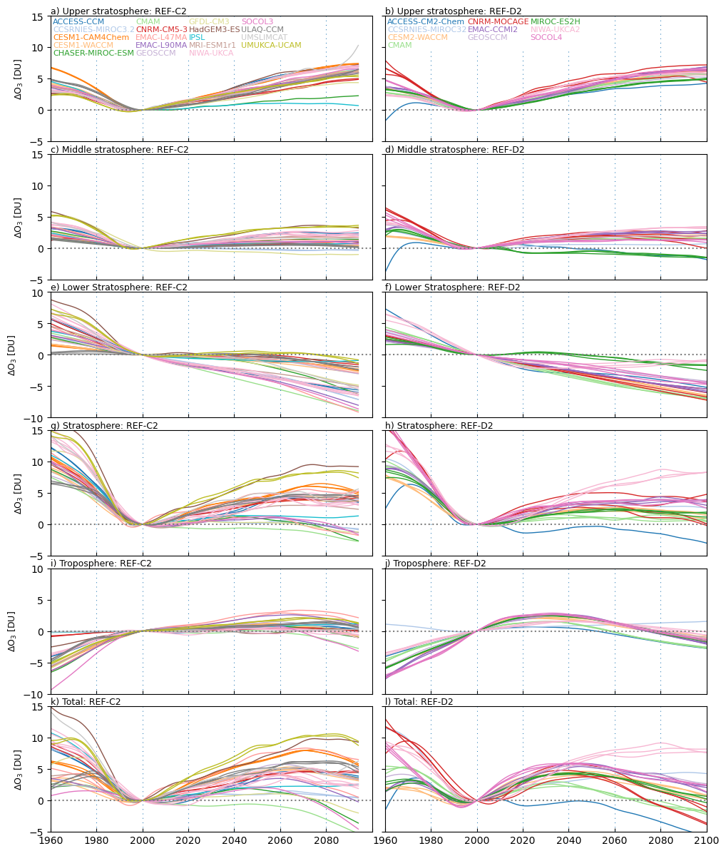
Figure 6 DLM background values over the “full period” (1960–2100) for REF-C2 simulations (left column) and REF-D2 (right column), relative to 2000 for (a) the upper stratospheric PCO, (b) middle stratospheric PCO, (c) lower stratospheric PCO, (d) whole stratospheric PCO, (e) tropospheric PCO, and (f) the TCO.

6 21st century tropical ozone changes

In this section, we consider changes in tropical ozone from DLM fits over the entirety of the REF-C2/REF-D2 simulations covering 1960–2100, but with a focus on 21st century behavior, the beginning of which roughly corresponds to the start of ODS-driven chemical ozone recovery. We note that while for the observational period (Sect. 5) the two scenarios should be very close, it is in the second part of the 21st century where the differences should become more apparent given the differing GHG emission scenarios used by the two experiments. The differences amount to an approximately 25 % reduction in 21st century CO₂ emissions in REF-D2 compared to REF-C2.

Figure 6 shows the DLM background trend timeseries in the various vertical layers in the stratosphere and troposphere, and Fig. 7 shows kernel density estimates of the DLM background trend change over the 21st century (2000–2094 for REF-C2 to cover the time period common to all models), similar to Fig. 5. These plots reveal generally consistent patterns of ozone changes across the two experiments and across models, but with a few notable exceptions discussed below.

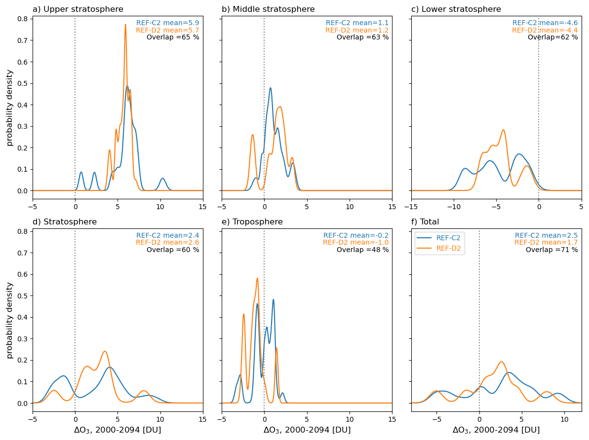
Figure 7 Kernel density estimates (KDEs) of DLM-based tropical ozone column change over 2000–2094 from REF-C2 (blue) and REF-D2 (orange) model simulations. The multi-model mean changes and overlap between the two experiments are indicated in each panel.

In the upper and middle stratosphere, ozone recovery is quite similar between the two experiments over the 21st century, with the CCMI experiments showing 63 % and 58 % overlap, respectively, and the bulk of ozone recovery (∼ 6 DU) coming from the upper stratospheric layer, as expected. In the tropical lower stratosphere, models robustly show an ozone decline throughout the 21st century, with a mean decrease of ∼ 5 DU and virtually no models showing positive changes. There is good overlap between the two CCMI experiments (59 %), but with a substantial spread among models within each experiment ranging from almost −10 DU to nearly zero.

Considering the stratosphere as a whole, the mean 21st century tropical ozone change is positive for both CCMI experiments (∼ 2–3 DU), but with substantial spread within and among the experiments. Notably, 6 REF-C2 models (CCSRNIES-MIROC3.2, CHASER-MIROC-ESM, CMAM, EMAC-L47MA, EMAC-L90MA, SOCOL3) and one REF-D2 model (ACCESS-CM2-Chem) have mean declines in stratospheric PCO over the 21st century. Of the REF-C2 models with negative changes, 5 of them comprise the most negative lower stratospheric PCO changes and range from −9 to −7 DU. The sixth model (CHASER-MIROC-ESM) has a lower stratospheric trend (−5.4 DU) close to the REF-C2 multi-model mean response (−4.9 DU), but has a significantly less positive upper stratospheric recovery (+2.2 DU, compared to the CCMI-1 mean of +6.3 DU) that contributes to its negative PCO trend for the whole stratosphere.

In contrast to REF-C2, where the models with negative stratospheric changes are largely those with the most negative lower stratospheric changes, the outlying negative stratospheric trend in the REF-D2 ACCESS-CM2-Chem simulation (Fig. 6h) is primarily due to its outlying negative trend in the middle stratosphere (Fig. 6d) which is not fully offset by its relatively weak positive trend in the upper stratosphere (Fig. 6b). Specifically, its combined middle/upper stratosphere trend is +2.6 DU, compared with the REF-D2 multi-model mean of +7.2 DU. In contrast, the ACCESS lower stratosphere trend is −4.9 DU, which is near the REF-D2 multi-model mean of −4.6 DU.

Over the 21st century, the multi-model mean tropospheric column ozone changes are different between the two model experiments, with a slightly negative trend in REF-D2 (−1.1 DU) and almost no decrease in REF-C2 (−0.2 DU). These results are opposite of the response over the first two decades of the 21st century, where REF-D2 shows an increase (+1.6 DU) and REF-C2 shows relatively little change (+0.3 DU).

7 Can observational period changes predict future changes?

In this section and the next one, we examine the degree to which tropical stratospheric ozone trends vary systematically across different time periods in models and observations, the extent to which these relationships might serve as an emergent constraint on model projections, and the feasibility and limitations of using existing observations to provide guidance on the credibility of model projections for a given emissions scenario. The motivating hypothesis for analyzing model ozone trends across time periods is that biases in ozone-controlling processes may lead some models to have stronger (or weaker) ozone trends that end up being correlated over different time periods. For example, a model that accelerates the BDC too strongly in response to GHG increases may show a too-negative lower stratospheric ozone trend during both the 20th and 21st centuries. Or in the upper stratosphere, a model that is overly sensitive to chlorine changes might show both a too-rapid depletion of ozone in the late 20th century and a too-rapid recovery in the 21st century.

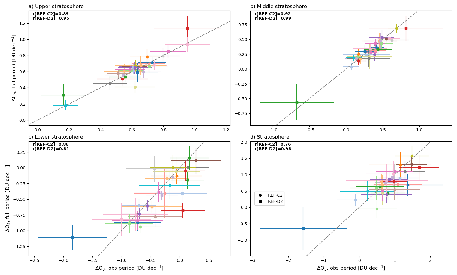
Figure 8 Scatter plots of model tropical partial column ozone trends (2000–2021 for lower stratosphere, turnaround–2021 for all others) for the DLM run with data from the full time period (1960–2100, y-axes), vs. for the DLM run with data only over the observational period (1985–2021). Each marker shows the DLM-inferred trend from a given model, with different symbols for different model experiments (see legend) and different colors for each model (see legends in Figs. 4 and 6). Horizontal and vertical error bars represent the ± 1 standard deviation about the mean DLM change, as in previous figures. The inter-model correlation coefficients (all of which are significant) for each multi-model experiment are shown in each panel, as are the 1:1 lines (gray, dashed).

For this analysis, we consider three time periods: the depletion period (before the turnaround, which occurs around 2000), the early 21st century recovery period (turnaround–2021), and the remainder of the 21st century (2022 and beyond). The key question we seek to answer in this section is whether or not the simulated later 21st century trends for a given scenario are correlated with modeled trends over the earlier periods encompassing available observations (∼ 1980–2021). Before doing that, we first test whether trends computed from input over short (one to two decade) time periods can accurately quantify the “true” model trends (i.e., those based on using the entire model time series as input to the DLM), as this is a necessary precondition for having confidence in any comparison between observations and models. Then, we explore inter-model correlations using different pairs of time periods to establish (1) how ozone depletion and early recovery trends covary across models, and (2) how late 21st century model trends covary with early 21st century recovery. The results from the latter of these tests establish the extent to which DLM trends from observations might provide some constraint on future model ozone projections. Then, in the following Sect. 8, we use the observational trends from Sect. 5 to assess the current ability to provide an observational constraint on 21st century tropical ozone trends.

7.1 Diagnosing trends over the observational period

In this section, we consider how well trends can be characterized over shorter time periods, such as the first few decades of the 21st century (comprising the early recovery period, i.e. turnaround to 2021). We address this issue by comparing 2000–2021 DLM trends from runs where the DLM is fed CCM output only from the observational time period (1985–2021) with 2000–2021 DLM trends from runs where the DLM uses data from the full time period of the model simulations (1960–2100). The latter of these is assumed to represent the “true” model trend that is unaffected by the limited sampling and endpoint issues that could potentially impact a shorter observational data record of only a few decades. Figure 8 shows the correlation between trends computed over the early 21st century recovery time period, with the only difference being the length of the data used as input to the DLM. As can be seen from this figure, the correlation between the two versions of the DLM are high for all regions of the stratosphere and for both multi-model experiments, and the models lie along the 1:1 line as expected. We note that excluding outliers (i.e., CHASER-MIROC32 in the middle stratosphere, ACCESS-CM2-Chem in the lower stratosphere and whole stratosphere) does not significantly alter the correlation coefficients. These results suggest that the true long-term trends over relatively short periods such as two decades can be accurately quantified from data records of limited length, and therefore lends confidence to the comparison of trends between observational datasets (whose data length is necessarily limited) and those from models.

7.2 Depletion vs. recovery period changes

We next consider the correlation between ozone trends over the depletion and recovery periods across models, separated by different vertical regions of the stratosphere. For regions of the stratosphere with a well defined turnaround (minimum) in their PCO time series (i.e., upper stratosphere, middle stratosphere, and whole stratosphere), we define the time boundary between the depletion and recovery periods as the date of the minimum in the DLM background trend occurring between 1990 and 2015. This turnaround date is identified separately from each of the 5000 DLM samples, for each timeseries (i.e., each combination of model realization and vertical region). Since there is in general no turnaround in ozone trend in the lower stratosphere, for this region the year 2000 is used. The turnaround date can vary significantly across each model realization and vertical region of the stratosphere, as well as to some degree across each of the 5000 DLM samples. As an example, the REF-C2 multi-model mean turnaround time is 1997 for the upper stratosphere (with range 1994–2010), but is delayed to 2002 for the whole stratosphere (with range 1996–2029).

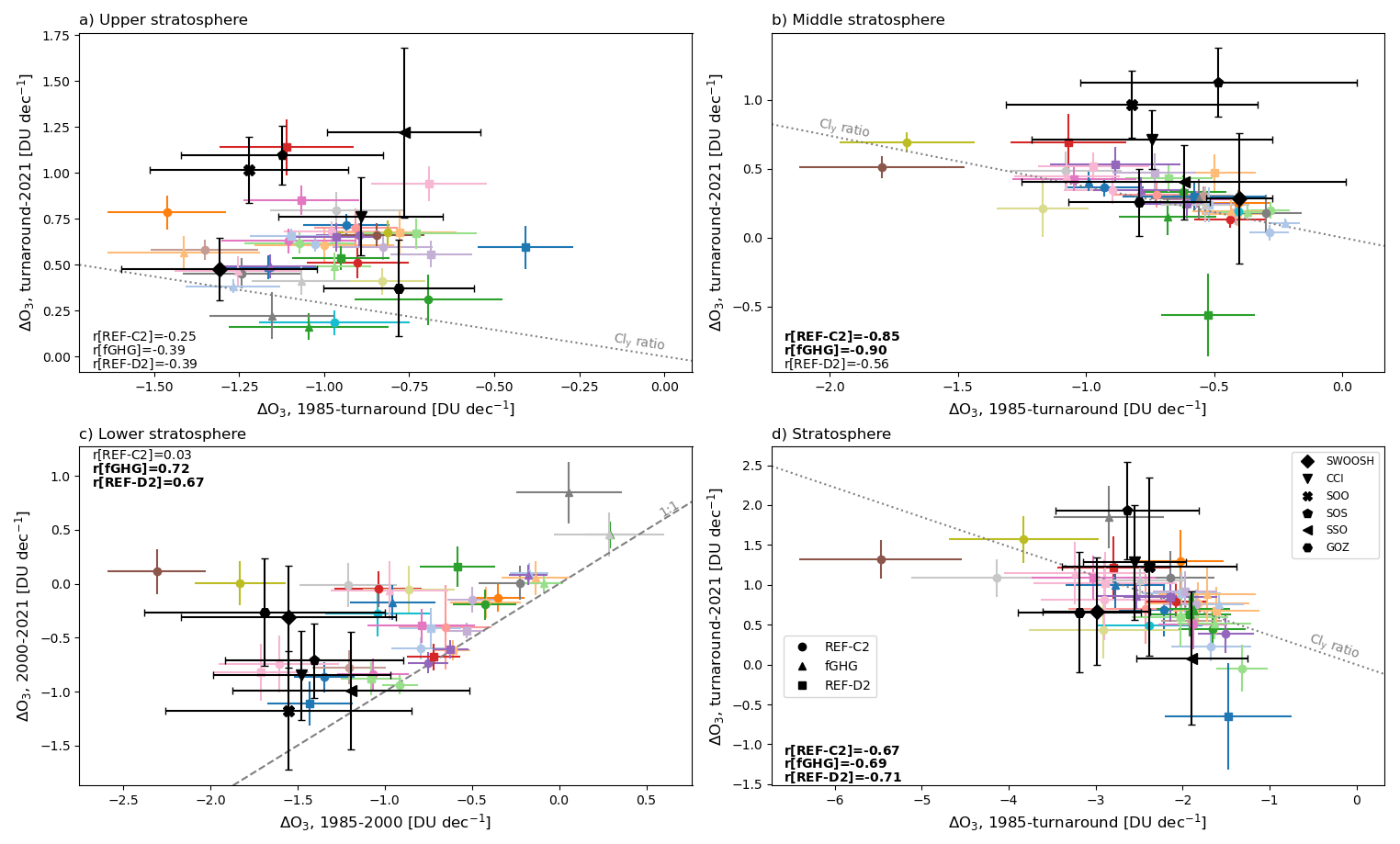
Figure 9 Scatter plots of the tropical partial column ozone depletion (horizontal axes) and early recovery (vertical axes) trends from models and observations. Each model marker shows the DLM-inferred trend from a single model realization, with different symbols for different model experiments (see legend) and different colors for each model (see legends in Figs. 4 and 6). Horizontal and vertical error bars indicate ± 1 standard deviation about the mean DLM change, as in previous figures. The inter-model correlation coefficients for each multi-model experiment are shown in each panel (significant correlations are in bold). The dotted gray lines in (a), (b), (d) show the multi-model mean value of the Cl_y recovery/depletion trend ratio calculated over the same latitude (30° S–30° N) and vertical region from the REF-C2 experiment. The dashed gray line in (c) is the 1:1 line, indicating values for which the LS PCO trends are the same both before and after 2000.

Figure 9 shows the inter-model correlation of trends over the depletion (1980–turnaround) and early 21st century recovery periods (turnaround–2021). This plot shows significant inter-model correlations between the strength of depletion and recovery for the whole stratosphere across all model experiments. Perhaps surprisingly, in the upper stratosphere the correlation across the models between depletion and early recovery trends is not significant. One might expect that models with shorter CFC lifetimes have both a faster inorganic chlorine (Cl_y) increase before and a faster Cl_y decrease after the peak Cl_y in the late 1990's, and that this behavior might lead to those same models having both faster ozone depletion and faster ozone recovery. To test this hypothesis, we consider the Cl_y trend ratio, which we define as the ratio of the tropical mean (30° S–30° N) Cl_y recovery trend (from peak Cl_y year to 2021) to the tropical mean Cl_y depletion trend (1985 to peak Cl_y year) calculated using Cl_y partial column amounts over the vertical region of interest (e.g., upper stratosphere) from each REF-C2 experiment. Compared to the REF simulations, ozone trends in the fGHG simulation (triangles, Fig. 9a) are generally closest to the multi-model mean Cl_y trend ratio (dotted line, Fig. 9a). This general agreement between the fGHG ozone trend ratios and the Cl_y trend ratios in the upper stratosphere makes sense given the “purely chemical” perturbations in the fGHG simulations, and the absence of complicating factors such as GHG-induced cooling and its associated knock-on effects on ozone. Indeed, almost all REF-C2 and REF-D2 models show stronger ozone recovery than that suggested from the Cl_y ratio (i.e., they are above the line in Fig. 9a), qualitatively in line with the fact that in the recovery period GHG and ODS both act to increase ozone, whereas in the depletion period the GHG forcing acts to offset the ODS forcing in the upper stratosphere.

In the middle stratosphere (Fig. 9b), there is a remarkably good correlation between ozone depletion and recovery rates for the two CCMI-1 experiments (i.e. REF-C2 and fGHG), whereby models with more rapid depletion also show more rapid recovery. The ozone recovery/depletion trend ratios in this region are in general agreement with the multi-model mean Cl_y ratio (gray dotted line, Fig. 9b), suggesting a rather straightforward connection between Cl_y changes and ozone changes in this region, and also potentially allowing for the use of an observational constraint on model projections. Although the REF-D2 correlation in Fig. 9b is not significant, we note that if the outlier model is removed (MIROC-ES2H), the correlation becomes significant for that experiment as well ($r=-\mathrm{0.70}$). The MIROC-ES2H model exhibits a dry bias in stratospheric water vapor due to a cold bias in the tropical upper troposphere and lower stratosphere. Excessive NO_x and associated catalytic reactions in the middle stratosphere lead to underestimated ozone, with differing ozone trends possibly linked to biases in nitrogen partitioning. It is possible that these biases may lead to the outlier behavior of this model in Fig. 9b.

In the lower stratosphere (Fig. 9c), there is a significant positive correlation of ozone trends between the pre- and post-2000 periods in the fGHG and REF-D2 experiments, in contrast to the negative correlations for other regions of the stratosphere. Given the predominately dynamical control over ozone in the lower stratosphere (with ozone changes driven predominantly by the GHG-induced acceleration of the BDC), this positive correlation is unsurprising and simply shows that, to some degree, models with stronger ozone trends in the first half of the observational time period tend to have stronger trends in the latter half (and vice versa for models with weak trends). This spread of model responses illustrates the variety of model BDC sensitivity to combined ODS/GHG forcing. Indeed, many of the model trends in this region fall near the 1:1 line (i.e., their trends are identical during each period; dashed line, Fig. 9c), although they are generally above the line, indicating relatively less negative trends during the early 21st century when ODS decreases tend to oppose BDC changes.

Taken together, the full stratospheric PCO correlations are significantly negative for all experiments (Fig. 9d), as expected based on the dominant contribution from the middle stratosphere. This behavior suggests that overall, models that show stronger ozone declines during the depletion period tend to show stronger ozone increases in the few decades during the early recovery period.

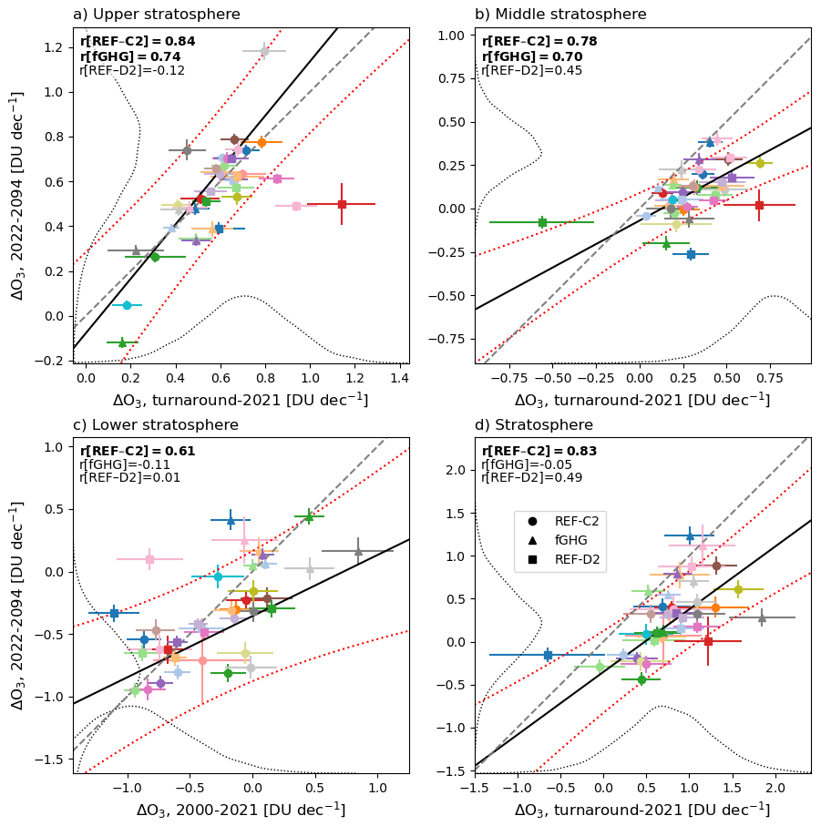
Figure 10 Scatter plots of the tropical partial column ozone early recovery (horizontal axes, 2000–2021) and later century (vertical axes, 2022–2094) trends. Each marker shows the DLM-inferred trend from a given model, with different symbols for different model experiments (see legend) and different colors for each model (see legends in Figs. 4 and 6). Horizontal and vertical error bars indicate the ± 1 standard deviation about the mean DLM change, as in previous figures. The intermodel correlation coefficients for each multi-model experiment are shown in each panel (significant correlations are in bold), as are the 1:1 lines (gray, dashed), the linear fit to the REF-C2 models (black lines), and their 95 % prediction interval (red dotted lines). Dotted black lines show the CCI dataset's DLM posterior trend distribution (along the horizontal axes) and the CCI-predicted late 21st century trends (along the vertical axes).

7.3 Observational period vs. late 21st century changes

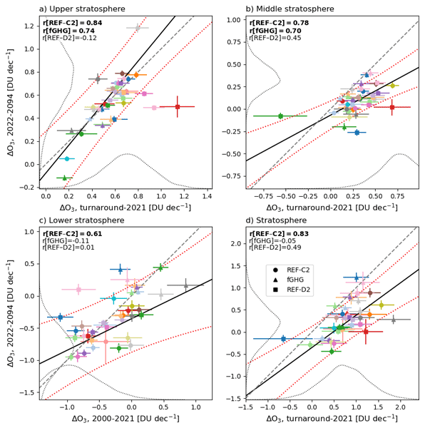
We next consider the inter-model correlation between trends for the beginning of ozone recovery (turnaround–2021) and the rest of the 21st century time period (2022–2094), based on DLM fits using data covering the whole 1960–2100 period as in the previous section (Fig. 10). At all levels, there is a significant inter-model correlation for REF-C2, whereby models with faster recovery in the first two decades also tend to show more positive trends over the rest of the 21st century. For the stratosphere as a whole (Fig. 10d), such correlation is not found for the other model experiments, a point which will be further discussed below. We also note that most models fall below the 1:1 line (dashed gray line, Fig. 10d), indicating that ozone trends in the later 21st century are mostly weaker than in the first two decades.

There are notable differences between the two generations of CCMI REF experiments throughout the stratosphere (Fig. 10a–c), with REF-C2 showing significant correlations at all levels, in contrast to the insignificant correlations in REF-D2. While diagnosing the exact mechanisms driving the differing correlations is beyond the scope of this analysis, we found that the differences between REF-C2 and REF-D2 are still present even when considering only the 10 models that have output from both experiments. Thus, it seems most likely that the difference in behavior is due to differing forcings (e.g., GHG forcing is weaker in REF-D2), or different representations of processes that might change through the 21st century (e.g., the QBO, Richter et al., 2020), or as-of-yet unidentified model biases.

In the middle and upper stratosphere, both REF-C2 experiments produce a significant positive correlation between early and late 21st century ozone trends, with REF-D2 showing borderline significant correlation in the middle stratosphere but very little correlation in the upper stratosphere. We note that unlike in Fig. 9b, removal of the outlier model in Fig. 10b does not change the correlation coefficient significantly. In the lower stratosphere, there is also a large difference in the correlations between REF-C2 (r=0.61) and REF-D2 (r=0.01). These results are somewhat surprising, given the expected GHG-induced strengthening of tropical upwelling in chemistry climate models and its impact on lower stratospheric ozone, in contrast to the multiple dynamical, chemical, and radiative processes that might influence middle stratospheric ozone.

In summary, in REF-C2 there is a strong positive correlation between model trends in the first two decades of the 21st century and the trends over the rest of the century in all layers of the stratosphere, whereas in REF-D2 there is a borderline significant correlation in the middle and whole stratosphere but insignificant correlations in the other layers. Except in the upper stratosphere, the model responses mostly lie below the 1:1 line, indicating that the trends over the later 21st century are generally smaller in magnitude than the first two decades of the century. At least for REF-C2, the early 21st century model ozone trends in the middle stratosphere appear to provide some “predictive” power for trends later in the century in that models with weak early-century trends also have weak late-century trends, and vice versa for models with strong trends.

8 Testing an observational constraint on future changes

Although a clear “emergent constraint” on end-of-century ozone trends is not robust in REF-D2 simulations, the robustness of the correlation between early 21st century and end-of-century ozone trends in REF-C2 models (particularly in the middle stratosphere) motivates further investigation of whether this relationship might be used in conjunction with early 21st century observations to provide an “observational constraint” on end-of-century values.

Figure 10 illustrates the application of an observational constraint for one dataset. The probability distributions along the horizontal axes of that figure show the DLM-inferred posterior trends from the CCI dataset (as in Fig. 5). This distribution is then convolved with the best-fit line (black line in Fig. 10) and its prediction interval (red dotted lines, Fig. 10) using a Monte Carlo sampling technique (see, e.g., Fig. 2, Nowack et al., 2023) to produce a CCI-informed late century trend on the vertical axis. The CCI-informed trend distribution can then be compared with the simulated end-of-century trends. In principle, if one believed the observations as “truth” and had strong correlations between early and late century model trends, one could interpret the difference between the CCI-informed late century trend and the multi-model trend as an indication of the multi-model bias for a given emissions pathway. However, the uncertainty of the observationally-informed late century trends (i.e., width of the distributions along the y axes in Fig. 10), which include contributions from both observational trend uncertainty (i.e., width of the distributions along the x axes in Fig. 10) and imperfect inter-model correlations (i.e., through the prediction interval), are in some cases (e.g., the upper stratosphere) too large to make such a straightforward assessment, even for a single observational data set. In this particular example, the CCI trend distribution agrees rather well with the whole-stratosphere trends from the models, but this agreement appears to be due to the models showing less positive trends than CCI in the middle/upper stratosphere (e.g., compare pdf along horizontal axis with model symbols in Fig. 10a–b) that are compensated for by more positive trends in the lower stratosphere.

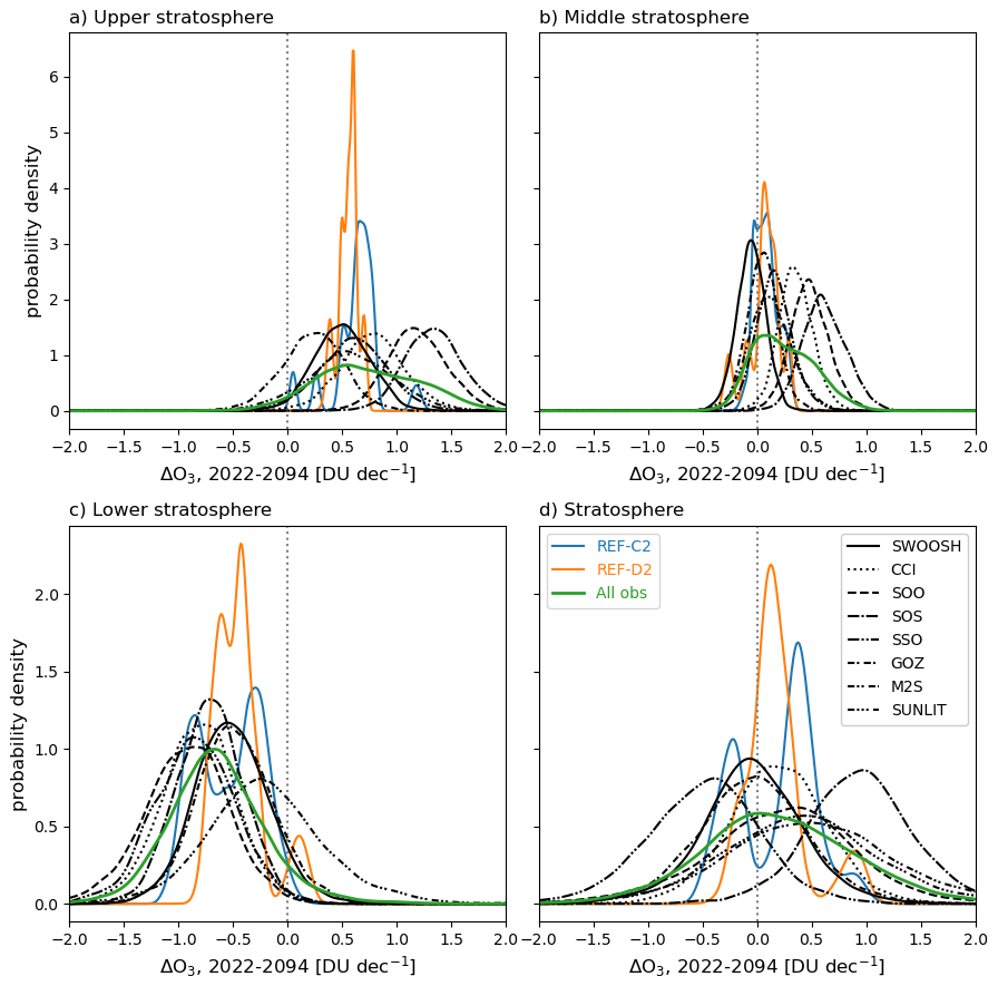
Figure 11 Kernel density estimates (KDEs) of tropical ozone column trends for 2022–2094 from REF-C2 (blue) and REF-D2 (orange) model simulations, as well as “observationally-informed” end-of-century trends constructed by combining observational trends over the early 21st century (2000/turnaround–2021, see Fig. 5) with the linear relationship between later and early century trends from REF-C2 in Fig. 10.

To evaluate how the available observations might agree (or not) with end-of-century values, we consider the distribution of observation-informed end-of-century values from a range of different data sources, using the method outlined above. Figure 11 shows the distribution of end-of-century trends based on the observations and the REF-C2 relationship, as well as the simulated trends. As expected, the spread amongst observational estimates (e.g., as seen in Fig. 5) is preserved in the (linear) transfer from early- to late-21st century trends. In the upper stratosphere, the widths of the observational distributions are generally greater than those of the models, whereas in the middle stratosphere, observations and model distribution widths are similar, suggesting that observationally-informed end-of-century trends are sufficiently precise to provide an observational constraint on the modeled trends in this region. However, in both regions systematic differences between the observational pdfs span a range that is larger than the width of the model distributions, and the conclusions one would draw about the accuracy of the model trends depends strongly on which observational estimate one regards as truth. For example, based on the SWOOSH data, one would conclude that the models systematically overestimate ozone trends in the middle and upper stratosphere, whereas one would conclude the opposite based on the SOO and SOS trends.

In contrast to the middle and upper stratosphere, for the lower (and whole) stratosphere the observationally-based distributions largely overlap one another but have widths that are significantly wider than the model distributions (Fig. 11c–d). The causes of the broader width of the observational distributions in the lower/whole stratosphere (Fig. 11c–d) compared to the middle/upper stratosphere (Fig. 11a–b) are both (1) wider prediction intervals (see Fig. 10) and wider observation-period trend distributions (see Fig. 5). Due to these wider distributions, observationally-informed end-of-century trends for the lower/whole stratosphere are limited in their ability to provide an observational constraint on the simulated trends, although most of the observational datasets would suggest that the models underestimate end-of-century trends in the lower stratosphere.

In the end, it is not possible to confidently apply an observational constraint on end-of-century ozone trends, although this analysis sheds some light on the potential for and current limitations of such an approach. First among these limitations is the wide spread amongst the observational estimates, which at some levels poorly overlap with one another and should motivate future studies aimed at reconciling these differences. Additionally, although there are plausible physical reasons for relationships between early and late century trends, inconsistencies between the results from different model generations reduce confidence in the robustness of these relationships. Recent work has documented significant differences in stratospheric transport among the two CCMI model generations discussed here (Abalos et al., 2026), although the specific impacts of these differences on emergent ozone behavior are not currently known.

9 Conclusions

In this study, we analyzed tropical total and partial column ozone trends in layers spanning the troposphere and stratosphere in multiple merged satellite datasets and chemistry-climate simulations from the REF-C2 and REF-D2 multi-model experiments. By applying dynamical linear modeling (DLM) to isolate background trends from natural variability, we assessed the consistency between simulated and observed ozone evolution over the observational time period (∼ 1980 to present), quantified 21st century model trends, and assessed the potential for the use of an observational constraint on future model trends.

Our results indicate that while both generations of CCMs simulate tropical TCO increases over the 2000–2021 period, the REF-D2 ensemble mean trend is more positive and in better quantitative agreement with observations than REF-C2. We find that the shift towards more positive TCO trends in REF-D2 is primarily due to a much stronger increase in tropical tropospheric ozone in REF-D2 (∼ 1.5 DU) compared to REF-C2 (∼ 0.3 DU) since 2000, likely driven by stronger increases in precursor emissions in REF-D2. For the stratosphere as a whole, PCO changes are nearly identical between the model experiments, although REF-D2 shows slightly more negative trends (by about 0.5 DU) in the lower stratosphere, which are compensated by more positive trends in the middle/upper stratosphere compared to REF-C2.

A major finding of this work is that substantial disagreement exists among observed tropical ozone trends over the past few decades, particularly in the troposphere and middle/upper stratosphere, and that these observational uncertainties critically limit our ability to evaluate the fidelity of CCMs in reproducing past changes. For example, in the upper stratosphere, observational estimates for the 2000–2021 period range from +0.6 to +2.6 DU, with minimal overlap between many of the datasets.

Similarly, estimates of tropospheric ozone changes range from negligible (SUNLIT) and in agreement with REF-C2, to strongly positive (TOMS+OMI/MLS) and in agreement with REF-D2, further complicating the validation of simulated trends. Ongoing work as part of the TOAR II activity is undertaking a more thorough intercomparison of satellite tropospheric column datasets, and their combined record generally supports the smaller end of the observational estimates presented here.

Despite these disagreements in the troposphere and middle/upper stratosphere, over 2000–2021 we find mostly significant negative lower stratospheric trends in observations that are on average more negative than those from both CCMI experiments. The CCMI multi-model mean ozone trends are negative (−0.6 DU for REF-C2, −1.1 DU for REF-D2), as are most of the DLM posterior trend distributions (69 % for REF-C2 and 77 % for REF-D2). These findings reinforce earlier findings of negative lower stratospheric ozone trends across multiple observational datasets (e.g., Ball et al., 2018; Godin-Beekman et al., 2022; Sofieva et al., 2026).

To understand how disagreements among currently available observations impact the future understanding of ozone, we examined the relationship between early 21st-century recovery trends and end-of-century trends in models. We found a robust inter-model correlation in all layers of the stratosphere for REF-C2, with a particularly strong correlation in the middle stratosphere (30–10 hPa). This suggests that models with faster early-recovery rates tend to project higher end-of-century ozone levels. However, this “emergent constraint” relationship is largely absent in REF-D2, except for a borderline significant correlation in the middle stratosphere. Although the reasons for this lack of correlation in the newer model simulations are not known, it is possible that they are due to differences in late-21st century forcing between the two REF experiments, the representation of dynamical processes such as the QBO that potentially change over the course of the century, or as-yet undiagnosed model biases.

Despite the presence of a relationship between recent and future ozone change in models, the practical application of an observational constraint is currently not possible. By propagating the spread of recent observational trends through the model-derived relationships, we demonstrated that the resulting uncertainty in “observationally-informed” end-of-century ozone is as large as, or larger than, the spread in the raw model projections. Depending on which observational dataset is treated as “truth”, one could conclude that models either systematically overestimate or underestimate stratospheric ozone recovery for a given emissions scenario.

Ultimately, these results indicate that uncertainties in recent tropical stratospheric and tropospheric ozone changes restrict our understanding of future total column ozone evolution. The current spread of observational trend estimates is insufficient for providing a robust constraint on future model projections. These results highlight a critical need for better reconciliation of observational ozone trend estimates among existing datasets, likely involving investigation of potential drifts in the source records that contribute to them, and further supports the utility of stable, trend quality stratospheric ozone measurements from both satellite and other platforms. Finally, the analysis here suggests a need to better understand inter-generational differences in chemistry climate models that lead to differing relationships between early and late 21st century ozone recovery.