Inferring European fossil fuel CO₂ emissions using TROPOMI NO₂ data and sector-based NO_x : CO₂ emission ratios

Accurate monitoring of fossil fuel CO₂ (ffCO₂) emissions is essential for tracking climate mitigation, yet natural carbon-cycle fluxes often obscure human-induced signals in atmospheric observations. This study presents a proof-of-concept satellite-driven data assimilation framework that uses nitrogen oxides (NO_x = NO + NO₂) – short-lived trace gases co-emitted with CO₂ –, to estimate ffCO₂ emissions. We estimate European NO_x emissions for 2021 by assimilating TROPOMI NO₂ observations into an Ensemble Kalman Filter (EnKF) framework, optimised within the GEOS-Chem atmospheric transport model. We use a computationally efficient offline treatment of NO_x chemistry, enabling large-ensemble inversions while retaining sensitivity to changes in photochemistry. Assimilating these data leads to a systematic reduction in the state vector uncertainty, with the mean uncertainty in total ffCO₂ emissions over Europe decreasing from 5.6 % in the prior to 3.3 % in the posterior. As well as overall improvement in model agreement with observations that corresponds to an annual correlation increase, Δr=0.12, derived from the correlation of all daily model–observation pairs across all grid cells in the European domain. By leveraging sector-specific NO_x : CO₂ emission ratios, we translate our posterior NO_x flux estimates into corresponding ffCO₂ estimates that capture enhanced seasonal variability. Our inferred ffCO₂ emissions exhibit elevated values in autumn and winter, spatially concentrated over major source regions and consistent with surface temperature variability. The inferred posterior adjustments include substantial increases in national emissions in several regions (20 %–91 % in national annual combustion CO₂), highlighting both the sensitivity of the method and the need for further validation and multi-species observational constraints. Independent evaluation against in situ measurements confirms significant improvements in mean error statistics in some regions. And updated national posterior ffCO₂ emissions show improved agreement with EDGAR across five high emitting European countries. This study demonstrates the potential of ensemble data assimilation and reduced-complexity chemistry to provide a first-order constraint on European ffCO₂ estimates, establishing a vital foundation for future joint NO₂–CO₂ inversion systems.

1 Introduction

Fossil fuel CO₂ (ffCO₂) emissions are the primary driver of anthropogenic climate change. Accurately monitoring these emissions is essential for tracking progress toward national mitigation goals. While national inventories and bottom-up emission datasets provide the primary basis for these assessments, atmospheric observation-based approaches offer a complementary, independent constraint. However, these top-down methods are complicated by the difficulty of isolating fossil fuel signals from large, seasonally varying biogenic fluxes. Top-down atmospheric inversions offer a way to improve emission estimates of ffCO₂, but in practice they remain limited by observational constraints and the inability to directly differentiate anthropogenic CO₂ from natural sources.

Studies are increasingly using atmospheric observations of trace gases co-emitted during combustion processes to infer ffCO₂ emissions (Meijer et al., 1996; Suntharalingam et al., 2004; Palmer et al., 2006; Lopez et al., 2013; Wenger et al., 2019; Super et al., 2020b; Miyazaki and Bowman, 2023). Nitrogen oxides (NO_x) are a leading candidate tracer to help infer ffCO₂ because they originate mostly from combustion and have a short atmospheric lifetime so that fresh emissions can be readily identified. High-resolution satellite observations of NO₂, such as those from TROPOMI, provide detailed patterns of emission activity. These measurements have been extensively used to infer NO_x emissions, either through mass balance methods (de Foy et al., 2015; Visser et al., 2019; Sun, 2022), comprehensive atmospheric inversions that account for transport and chemistry (Stavrakou et al., 2008; Gu et al., 2014; Itahashi et al., 2019; Plauchu et al., 2024; Kong et al., 2025), or hybrid approaches that combine elements of both (Qu et al., 2017, 2020). By applying sector-dependent emission ratios, it is then possible to infer spatial patterns of ffCO₂ from these NO_x emission estimates (Berezin et al., 2013; Lopez et al., 2013; Goldberg et al., 2019, 2024; Jia et al., 2025). Preliminary studies have assessed the ability of using synthetic atmospheric observations of both NO₂ and CO₂ in tandem to assess methodologies for more robust estimates of ffCO₂ flux (Kuhlmann et al., 2021; Kaminski et al., 2022; Santaren et al., 2025).

However, such a tracer-based approach is subject to substantial uncertainties. A key limitation is the uncertainty associated with the CO₂ and NO_x emission ratios, which vary by sector, fuel type, combustion technology, and emission control strategies (Jiang et al., 2010; Wang et al., 2025; Super et al., 2020a). Additional challenges include errors in atmospheric transport modelling, uncertainties in the representation of chemical processes controlling NO_x lifetimes, sparse and inhomogeneous observational coverage, and the difficulty of accurately estimating background concentrations (Peylin et al., 2013; Andrew, 2020). These factors complicate the interpretation of NO₂ columns and the propagation of information from observed concentrations back to surface emissions and, ultimately, to ffCO₂ fluxes. Data assimilation frameworks such as the Ensemble Kalman Filter (EnKF) provide a powerful means of addressing some of these challenges by explicitly representing and propagating uncertainties in emissions, chemistry, transport, and observations. These limitations mean that tracer-based approaches currently provide only indirect and approximate constraints on ffCO₂ emissions. In particular, assumptions regarding fixed NO_x : CO₂ emission ratios represent a key limitation for tracer-based approaches and can introduce systematic biases in inferred ffCO₂ emissions.

We present a methodology that uses TROPOMI NO₂ observations within an Ensemble Kalman Filter (EnKF) framework to infer daily NO_x emission estimates over Europe during 2021. Our approach uses the GEOS-Chem model with a novel, lightweight offline NO_x chemistry module, extending the work of Schooling et al. (2025). By embedding this reduced-complexity chemistry within an ensemble data assimilation system, we demonstrate a computationally efficient pathway for satellite-derived ffCO₂ estimation. In this framework, NO₂ observations are assimilated to constrain NO_x emissions, and ffCO₂ emissions are subsequently inferred diagnostically using prescribed NO_x : CO₂ emission ratios. Cross-species error correlations are represented in the prior covariance structure to represent shared uncertainties between NO_x and CO₂ emissions, but CO₂ fluxes are not directly optimised and are inferred post hoc from the optimised NO_x emissions. This framework establishes a scalable foundation for future joint inversions of NO₂ and CO₂.

In the next section, we describe the data and methods, including TROPOMI NO₂ data, the GEOS-Chem atmospheric chemistry transport and its configuration used for the experiments we report here that includes our offline NO_x chemistry module, and the ensemble Kalman filter. We also include details about the sector-based NO_x : CO₂ emission ratios used to translate our posterior NO_x emission estimates into ffCO₂ emission estimates. In Sect. 3, we describe our results. We conclude our study in Sect. 4.

2 Data and methods

2.1 Atmospheric NO₂ observations

We use satellite observations of NO₂ from the TROPOspheric Monitoring Instrument (TROPOMI) to constrain anthropogenic NO_x and CO₂ emissions over Europe. TROPOMI is a push-broom imaging spectrometer aboard Copernicus Sentinel-5 Precursor (S5P), launched in October 2017. S5P operates in a sun-synchronous Low-Earth Orbit at an altitude of approximately 824 km, with an ascending node local equator-crossing time of 13:30 LT. TROPOMI has an across track swath of 2600 km, resulting in a daily global coverage. The nadir spatial resolution for NO₂ was initially 7×3.5 km² and was further refined to 5.5×3.5 km² in August 2019. The NO₂ retrievals use the UV/Vis spectral range (405–465 nm), with typical uncertainties of order 10 %–40 % depending on viewing and atmospheric conditions (Veefkind et al., 2012; van Geffen et al., 2022). For our study, we use v2.4.0 of the Sentinel-5P TROPOMI Level-2 NO₂ data for the full year of 2021. We consider measurements that have a quality assurance value qa ≥ 0.75 to remove low-quality pixels (van Geffen et al., 2022).

To evaluate the NO_x posterior emission estimates inferred from TROPOMI NO₂ column data, and the corresponding ffCO₂ estimates, we use independent atmospheric NO₂ and CO₂ measurements. We use satellite observations of column-averaged CO₂ retrieved from the NASA Orbiting Carbon Observatory (OCO-2) to evaluate the influence of our posterior ffCO₂ emission estimates on the total column. We acknowledge fresh ffCO₂ emissions represent at most a few percent of the column quantity so that distinguishing the anthropogenic signal from the natural carbon cycle and background concentrations becomes a significant observational challenge. Despite this, the high precision of OCO-2 measurements (0.5 ppm; Jacobs et al., 2024) allows us to detect subtle enhancements in the total column over major industrial regions and urban centres (Schwandner et al., 2017; Ye et al., 2020). We use the Level 2 Lite Full Physics product retrieved using the Atmospheric CO₂ Observations from Space (ACOS) algorithm, version 10. These data provide bias-corrected, quality-screened XCO₂ retrievals with a footprint of approximately 1.3×2.25 km², acquired in nadir with a local overpass time of 13:30 LT. Due to OCO-2's narrow ∼10 km swath and strict cloud filtering, spatial coverage is sparse.

For consistency with our NO₂ filtering criterion, we select only high-quality retrievals with a quality assurance value qa ≥ 0.75. Both satellite datasets were resampled to the GEOS-Chem nested model resolution of 0.25° (latitude) × 0.3125° (longitude); the model is described below. Figure 1a shows the proportion of European grid points covered per day and per month for TROPOMI and OCO-2. Generally coverage is highest during summer months. To ensure accurate comparison with observations, we interpolate the satellite averaging kernels onto the 47 vertical levels of the model to compute vertically sensitive model column densities.

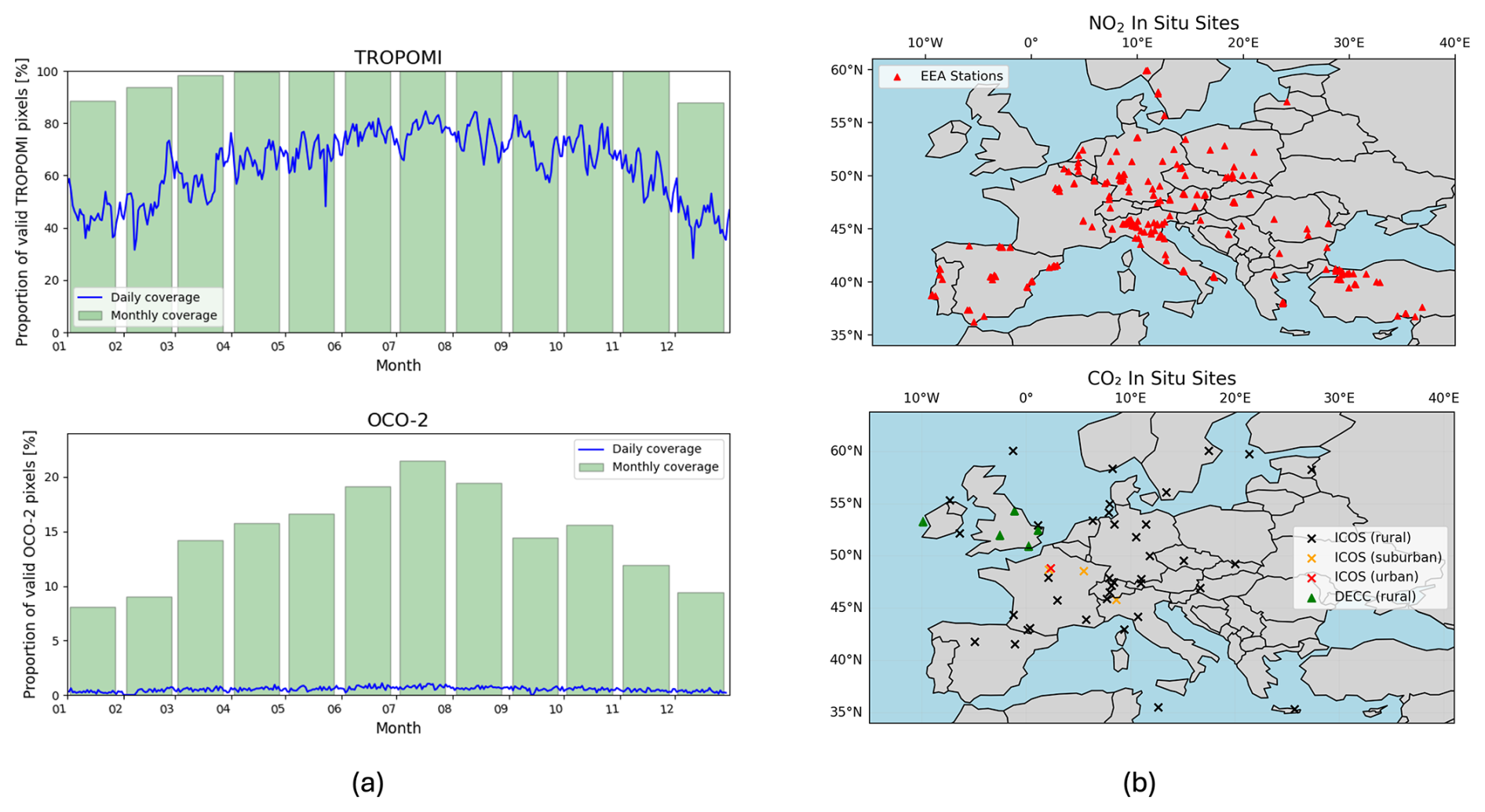
Figure 1 (a) The fractional daily and monthly European coverage of TROPOMI NO₂ (top panel) and OCO-2 (bottom panel). Coverage is defined as the fraction of GEOS-Chem model grid cells across the European domain that receive at least one clear-sky TROPOMI or OCO-2 observation within the specified time period. Thus, 100 % daily coverage means every model grid was observed at least once during the period (day or month). (b) Maps of the in situ observation sites used for evaluation. The top panel shows the locations of the 202 EEA NO₂ monitoring stations. The bottom panel shows the 47 in situ CO₂ measurement sites, including 5 DECC sites (green triangles) and 42 ICOS sites (crosses), with ICOS stations further classified by type (rural = black, suburban = yellow, urban = red).

We also used in situ measurements of NO₂ and CO₂ collected across Europe (Fig. 1b). We use NO₂ data from the European Environment Agency (EEA) air quality network (European Environment Agency and Heisig, 2025), including 202 sites across Europe that had at least 100 d of coverage in 2021. EEA data are processed using standardised quality filtering procedures, and data are reported with a mean uncertainty of ∼4 µg m⁻³ across rural and urban background areas (Horálek et al., 2023). We also used in situ measurements of CO₂ from multiple ground-based monitoring networks across Europe, including the Integrated Carbon Observation System (ICOS) (ICOS RI et al., 2025), and the UK's Department for Energy Security and Net Zero (formerly DECC) sites (Stanley et al., 2018).

2.2 The GEOS-Chem atmospheric chemistry transport model

We use the nested version of the GEOS-Chem atmospheric chemistry transport model (version 14.4.3) (Bey et al., 2001). The model is driven by offline meteorological fields from the GEOS-FP dataset provided by NASA's Global Modeling and Assimilation Office (GMAO), using the native horizontal resolution of 0.25°×0.3125°, 47 vertical levels (grouped from the native 72 levels), and 3-hourly temporal resolution. The forward model simulations used within the inversion framework use an adapted tagged CO₂ model configuration that includes a lightweight offline treatment of NO_x chemistry, described below.

The nested model is centred over mainland Europe (32.75 to 61.25° N, −15 to 40° E). Lateral boundary conditions to the European domain were created from a consistent global GEOS-Chem model run at 4°×5°, with three-hourly output fields. The nested model was run with a 5 min transport timestep and 10 min chemistry timestep.

Prior combustion emissions of NO_x and CO₂ are taken from the CAMS-REG v8.1 emissions inventory at 0.05°×0.1° resolution (Fig. 2) (Kuenen et al., 2022). CAMS-REG provides a high-resolution gridded emission dataset derived from a combination of country-reported inventories, activity statistics, and emission factors following established reporting frameworks (e.g. UNFCCC for greenhouse gases and EMEP for air pollutants). Country-level emissions are compiled across detailed sector and fuel categories and subsequently spatially disaggregated using proxy datasets such as population density, land use, transport networks, and point source information. As a result of this construction, spatial emission patterns often reflect national boundaries, due to differences in reporting methodologies, activity data quality, and emission factor assumptions between countries.

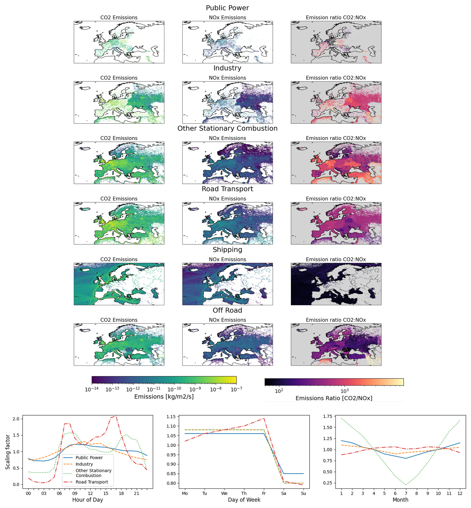
Figure 2 CAMS-REG v8.1 2021 emissions on the GEOS-Chem model grid (0.25°×0.3125°). Top panel shows CO₂ (left panels), NO_x (middle panels), and their ratio (right panels) for six main combustion sectors. The bottom panel shows the temporal profiles for Public Power, Industry, Other Stationary Combustion, and Road Transport.

Temporal variability in emissions (monthly, daily, hourly) is represented using sector-based scaling factors provided by TNO (Netherlands Organisation for Applied Scientific Research) (Fig. 2). Combustion sectors include public power, industry, road transport, ships, aviation, off-road machinery, and other combustion sources. Emissions from non-combustion sources in the CAMS-REG v8.1 inventory include fugitives, waste, solvents, and agriculture. We also prescribe NO_x emissions from soil and lightning, which are parameterised within GEOS-Chem (Vinken et al., 2014; Gressent et al., 2016). All non-combustion sources of NO_x are kept fixed at their prior values as they are not directly coupled to the NO_x–CO₂ relationship considered in this study. For non-fossil-fuel CO₂ sources and sinks we use the CarbonTracker Europe High Resolution (CTE-HR) inventory (van der Woude, 2022), which combines the SiB4 biosphere model v4.2-COS for net ecosystem production (NEP), GFAS fire emissions, and Jena CarboScope ocean fluxes at a 0.5°×0.5° resolution.

To efficiently and effectively incorporate NO_x into our model, we use the methodology presented in Schooling et al. (2025). In that work, we found that for unchanged meteorological conditions but varying emissions, the instantaneous NO_x chemical rates of change can be estimated by scaling the baseline (unperturbed, or prior) rate of change, $R^{\mathrm{B}}(x,y,z,t)$ by the relative change in local NO_x concentration, [NO_x]^′/[NO_x]^B, where [NO_x]^′ is the new concentration and [NO_x]^B is the baseline. This reproduces the NO_x chemical rates of change with high fidelity (R²=1.0). We use the GEOS-Chem full-chemistry simulation to generate hourly offline fields for the baseline NO_x concentrations, [NO_x]${}^{\mathrm{B}}(x,y,z,t)$] and instantaneous NO_x net chemistry rates, $R^{\mathrm{B}}(x,y,z,t)$.

For all additional model runs within the data assimilation procedure, we use the carbon model, where NO_x was introduced as a new tracer species. We read in these offline fields and calculate the updated NO_x chemistry net rate of change, $R\mathrm{\prime }(x,y,z,t)$ for each grid point ($x,y,z$) and time step (t):

$$\begin{array}{}\text{(1)}& R^{\prime }(x,y,z,t)=R^{\mathrm{B}}(x,y,z,t){\displaystyle \frac{{\left[{\mathrm{NO}}_x\right]}^{\prime }(x,y,z,t)}{{\left[{\mathrm{NO}}_x\right]}^{\mathrm{B}}(x,y,z,t)}}.\end{array}$$

We include the NO_x chemistry into the carbon-only simulation through the Kinetic PreProcessor (KPP) mechanism, which describes the production and decay processes of NO_x using the updated calculated rates of change. Additionally, since the partitioning NO₂ : NO_x was found to be stable under emission perturbations (Schooling et al., 2025), we store offline fields of the partitioning ratio at each grid point from full chemistry runs, enabling the conversion of simulated NO_x concentrations to NO₂ columns for comparison with TROPOMI observations.

The offline NO_x chemistry scheme has previously been validated for moderate (20 %) emission perturbations (Schooling et al., 2025). In this study, we extend this validation to the larger perturbations encountered in the inversion by comparing the offline parameterisation against full GEOS-Chem chemistry for representative days in each season. This analysis (Fig. A1) shows that the offline scheme accurately reproduces NO_x chemical loss rates (R²>0.94) and preserves the stability of the NO₂ : NO_x partitioning (R²=1), supporting its use across the range of perturbations considered here.

2.3 Ensemble Kalman Filter

We use an existing EnKF framework that has been widely used to estimate CO₂ and methane fluxes from atmospheric data (Feng et al., 2009; Zhu et al., 2022; Feng et al., 2017; Palmer et al., 2019; Feng et al., 2022; Zhu et al., 2025; Feng et al., 2025). The ensemble approach simplifies the calculation of these matrices by approximating the background error covariance matrix (P^f) through a finite sample of model realisations and avoids the needs to calculate an adjoint model.

We introduce an ensemble of N=100 perturbation states. The ensemble approach represents uncertainty in the state vector using a set of model realisations, from which the ensemble mean and perturbations are used to approximate the background error covariance. In our implementation, we use the EnKF to assimilate satellite observations of NO₂ column (y_obs), to update prior knowledge of our state vector, NO_x emission scaling factors (x^f), resulting in posterior scaling factor estimates (x^a):

$$\begin{array}{}\text{(2)}& {\mathit{x}}^{\mathrm{a}}={\mathit{x}}^{\mathrm{f}}+\mathbf{K}\left[{\mathit{y}}_{\mathrm{obs}}-H\left({\mathit{x}}^{\mathrm{f}}\right)\right],\end{array}$$

where H is the observation operator that maps the state vector to observation space, which comprises the GEOS-Chem model to relate changes in NO_x emissions to changes in atmospheric NO₂ with the resulting profiles sampled at the time and location of TROPOMI observations and subsequently convolved with scene-dependent averaging kernels.

K is the Kalman gain matrix and is given by:

$$\begin{array}{}\text{(3)}& \mathbf{K}\approx \mathrm{\Delta }{\mathbf{X}}^{\mathrm{f}}{\left(\mathrm{\Delta }{\mathbf{Y}}^{\mathrm{f}}\right)}^T{\left[\mathrm{\Delta }{\mathbf{Y}}^{\mathrm{f}}{\left(\mathrm{\Delta }{\mathbf{Y}}^{\mathrm{f}}\right)}^T+\mathbf{R}\right]}^{-\mathrm{1}},\end{array}$$

where ΔX^f represents the ensemble of deviations from the prior ensemble mean in state space and ΔY^f represents the corresponding ensemble of deviations in the observation space. These quantities are constructed from the ensemble perturbations of the state vector and their mapped equivalents in observation space.

To reduce the impact of spurious long-range correlations, we applied localisation to the Kalman gain. We compute the distance between each grid cell (d_ij) and each valid observation, and apply a Gaussian tapering function $\exp (-d_{ij}/l)$ with a decorrelation length scale l=200 km. This localisation is applied multiplicatively to the Kalman gain, element-wise.

For our study, we define R as a diagonal matrix that incorporates satellite retrieval uncertainty using the TROPOMI precision values, and includes a fixed model error of 1×10¹³ molec. cm⁻², corresponding to the average reconstruction error of NO₂ columns derived from scaled offline chemistry (Schooling et al., 2025). We also employed an adaptive inflation scheme that increased the observation error variance (diagonal elements of R) by a factor of 10 whenever the absolute value of the innovation surpassed a significant threshold ($\left|\mathit{d}\right|>\mathrm{1}\times {\mathrm{10}}^{\mathrm{16}}$ molec. cm⁻²).

The ensemble error covariance is derived using our understanding of the CAMS-REG v8.1 emission uncertainties (Super et al., 2026) as well as the error correlation between the two species. The cross-species error correlation (ρ) is a global product developed under the CORSO project. It is based on the assumption that the error correlation between NO_x and CO₂ occurs from their shared activity data, whereas the emission factor errors are independent. For each emission sector the uncertainties in the activity data (including spatial disaggregation) and emission factors are estimated from the IPCC guidelines (CO₂) (Eggleston et al., 2006), the EMEP guidebook (NO_x) (Nielsen, 2013) and information on the spatial disaggregation of the global EDGAR emission inventory (European Commission, Joint Research Centre, Institute for Environment and Sustainability, 2012). Since these uncertainties are defined per fuel type, information on the fuel mix per country (BP, 2022) is used to aggregate these uncertainties. A look-up table is created that lists the error correlation as a function of the sectoral uncertainty in activity data and emission factors. The higher the uncertainty in the activity data, the larger the cross-species error correlation.

The ensemble background error covariance matrix (P^f) was constructed using the NO_x and CO₂ flux uncertainties (σ_n, σ_c) together with the cross-species error correlation (ρ):

$$\begin{array}{}\text{(4)}& {\mathbf{P}}^{\mathrm{f}}=\left(\begin{array}{cc}{\mathit{\sigma }}_n^{\mathrm{2}}& \mathit{\rho }{\mathit{\sigma }}_n{\mathit{\sigma }}_c\\ \mathit{\rho }{\mathit{\sigma }}_n{\mathit{\sigma }}_c& {\mathit{\sigma }}_c^{\mathrm{2}}\end{array}\right),\end{array}$$

where the values of σ_n, σ_c and r are prescribed from the CAMS-REG v8.1 uncertainty estimates and the CORSO cross-species correlation product, and are assumed to be constant in time (i.e. no seasonal dependence). Emission errors are represented using a spatially correlated prior ensemble. Spatial correlations in the prior ensemble are based on the sector-specific correlation lengths provided by the CAMS-REG uncertainty dataset. These correlation lengths vary by emission sector (typically ranging from ∼20 to 80 km), reflecting differences in the spatial representativeness of emission sources. Given the use of a 1 d assimilation window, temporal correlations in emission errors are not represented in the prior error covariance. Emission errors are therefore treated as independent between successive days.

We generate a prior ensemble of NO_x emission scalings by sampling from a bivariate normal distribution, 𝒩(0,P^f) at each grid cell. This produces spatially resolved perturbations that preserve both the magnitude of uncertainties and the correlation between NO_x and CO₂ errors (Fig. 3).

Figure 3 NO_x and CO₂ uncertainties (σ_n, σ_c) from CAMS-REG v8.1 emissions (Super et al., 2026), the CORSO cross-species error correlation product (ρ), and the prior error defined as the ensemble-based standard deviation of the emission perturbations derived from sampling the prior error covariance matrix (P^f). All panels share a common colour scale for ease of comparison. The uncertainty fields (σ_n, σ_c, and the combined prior ensemble error) are expressed as relative standard deviations (dimensionless, defined as $\mathit{\sigma }/E$), while the correlation field (ρ) is also dimensionless, representing the correlation coefficient between NO_x and CO₂ errors.

The forward-modelled NO₂ columns from each ensemble member (H(x^f)) are compared to satellite retrievals to compute the innovation vector $\mathit{d}={\mathit{y}}_{\mathrm{obs}}-H\left({\mathit{x}}^{\mathrm{f}}\right)$. We restrict this comparison to grid cells that include valid satellite data (qa > 0.75). A spatial mask is applied to exclude edge regions and unphysical retrievals. Edge regions correspond to the outer two GEOS-Chem grid boxes of the domain, and retrievals with NO₂ columns greater than 1×10¹⁷ molec. cm⁻² are removed as nonphysical.

Since NO_x is short-lived, observations are generally insensitive to emission changes from previous days so we use a data assimilation window of 1 d. At the end of each assimilation cycle, the posterior emission scaling factors are applied to update the model state through the GEOS-Chem restart file, which is then used to initialise the next day's simulation. Sensitivity tests (Fig. A3) show that perturbations introduced through these restart adjustments have a negligible impact on simulated NO₂ columns by the second day, indicating that the observations are primarily sensitive to emission changes occurring within the previous day.

Due to the non-linear relationship between NO_x emissions and atmospheric NO₂, it is possible to maximise error reduction by repeating the ensemble runs multiple times in an iterative data assimilation procedure. Up to four iterations were performed, however the procedure is broken early if the percentage reduction in mean absolute error (MAE) falls below 1 %, suggesting a plateau in model improvement.

The posterior flux time series can exhibit relatively strong day-to-day variability, likely driven by gaps and inhomogeneities in the observational coverage that introduce intermittent and uneven constraints within the EnKF system. Additional contributions may arise from underestimated observation or model–data mismatch uncertainties, retrieval artefacts, and transport model errors, which can introduce high-frequency noise into the posterior solution. To reduce this noise and to better isolate robust temporal signals, we apply a Savitzky–Golay filter to the posterior emission estimates using a 5 d window and a third-order polynomial (Chen et al., 2004).

2.4 Conversion of NO_x scaling factors to CO₂ flux adjustments

The inference of ffCO₂ emissions from posterior NO_x fluxes relies on the use of prescribed CAMS-REG NO_x : CO₂ emission ratios that vary by sector and spatial location but are assumed to be temporally invariant. CO₂ emissions are therefore inferred diagnostically from the posterior NO_x emissions, rather than being directly optimised within the EnKF framework. In practice, this is implemented by applying the posterior NO_x scaling factors uniformly to co-located combustion-related CO₂ emissions at each grid cell, implicitly assuming a fixed sector-weighted NO_x : CO₂ ratio determined by the relative contributions of individual sectors within that grid cell.

The prior error covariance matrix P^f is constructed using prescribed uncertainties for NO_x (σ_n) and CO₂ (σ_c) emissions, together with a cross-species error correlation (ρ). This defines a prior uncertainty structure in which NO_x and CO₂ emissions exhibit correlated variability, reflecting their shared dependence on underlying activity data and emission factors. However, CO₂ emissions are not included in the inversion state vector and are therefore not directly optimised. The cross-species correlation is used only to represent consistent prior assumptions about the relationship between NO_x and CO₂ uncertainties, rather than implying an explicit propagation of CO₂ uncertainty through the inversion.

The assumption of temporally fixed emission ratios may introduce systematic biases in the inferred CO₂ emissions. In addition, any inaccuracies in the underlying CAMS-REG estimates of these emission ratios will propagate directly into the inferred CO₂ fluxes. We therefore treat this assumption as a central limitation of the present framework and acknowledge its implications when interpreting the results.

2.5 Statistical metrics for uncertainty and model performance

To quantify the reduction in uncertainty within the ensemble we calculate the ensemble-based error reduction (ER):

$$\begin{array}{}\text{(5)}& \mathrm{ER}=\mathrm{100}\times \left(\mathrm{1}-{\displaystyle \frac{{\mathit{\sigma }}_{\mathrm{post}}}{{\mathit{\sigma }}_{\mathrm{pri}}}}\right),\end{array}$$

where, σ_pri and σ_post are the prior and posterior ensemble standard deviations, respectively. To quantify the model agreement with observations between our prior and posterior emission estimates, we assess the pearson correlation coefficient (r), the mean bias, and the mean absolute error (MAE).

3 Results

In this section, we report our posterior European NO_x emission estimates and the corresponding ffCO₂ estimates for 2021, and the evaluation of the resulting posterior atmospheric NO₂ and CO₂ mole fractions at sites over the GEOS-Chem European domain (which includes parts of continental Europe and North Africa).

3.1 Inversion results

We find that our inversion leads to a systematic reduction of the state vector uncertainty, with mean ensemble-based Europe-wide error reductions of 5.7 %, 4.7 %, 4.2 %, and 4.6 % during DJF, MAM, JJA, and SON, respectively (Fig. 4). These values are calculated from daily error reduction fields at the model grid-cell resolution (0.25°×0.3125°), averaged over each season and subsequently across the European domain. This result demonstrates that TROPOMI NO₂ column data provide effective constraints on NO_x emission estimates, even though we have reasonable bottom-up inventory knowledge. We note that the larger uncertainty reductions occur over major emission regions such as London, Paris, Madrid – as well as in North Africa, where the prior ensemble spread is highest (Fig. 3).

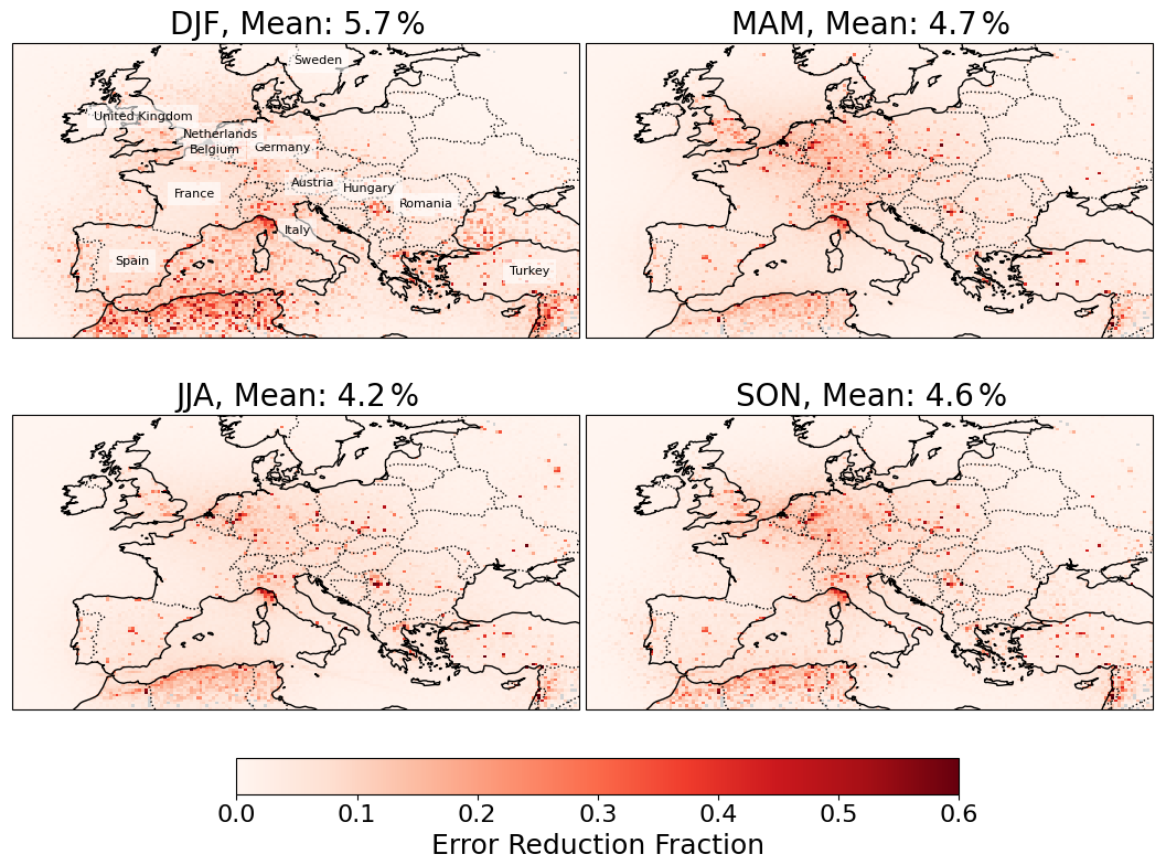
Figure 4 Seasonal maps of the mean ensemble based error reduction (Eq. 5). Error reduction is computed at the native model resolution (0.25°×0.3125°) and daily time step from the ratio of posterior to prior ensemble spread. Seasonal values are obtained by averaging these daily error reduction fields over each season (DJF, MAM, JJA, SON). Reported mean values represent spatial averages over all grid cells within the European domain. The locations of the 12 high emitting countries are labelled in the first panel.

These posterior updates also translate into a general improvement in model minus observation agreement, with an annual increase in Pearson r from 0.42 to 0.54, a reduction in mean absolute error of 1×10¹⁴ molec. cm⁻², and an overall improvement in the negative bias by 6×10¹³ molec. cm⁻². Figure 5a shows the prior and posterior model agreement for each month of the year. The correlation exhibits a modest increase in every month. MAE decreases in all months apart from July, where the prior error was already small, and the negative bias improves in all months apart from May, June, and July, where the prior bias was again already small. Overall the magnitude of these changes remains modest when aggregated across the full domain. This reflects the fact that model–observation mismatch is influenced by factors beyond emission errors alone, including boundary conditions, and initial concentrations, which are not directly constrained within the inversion framework.

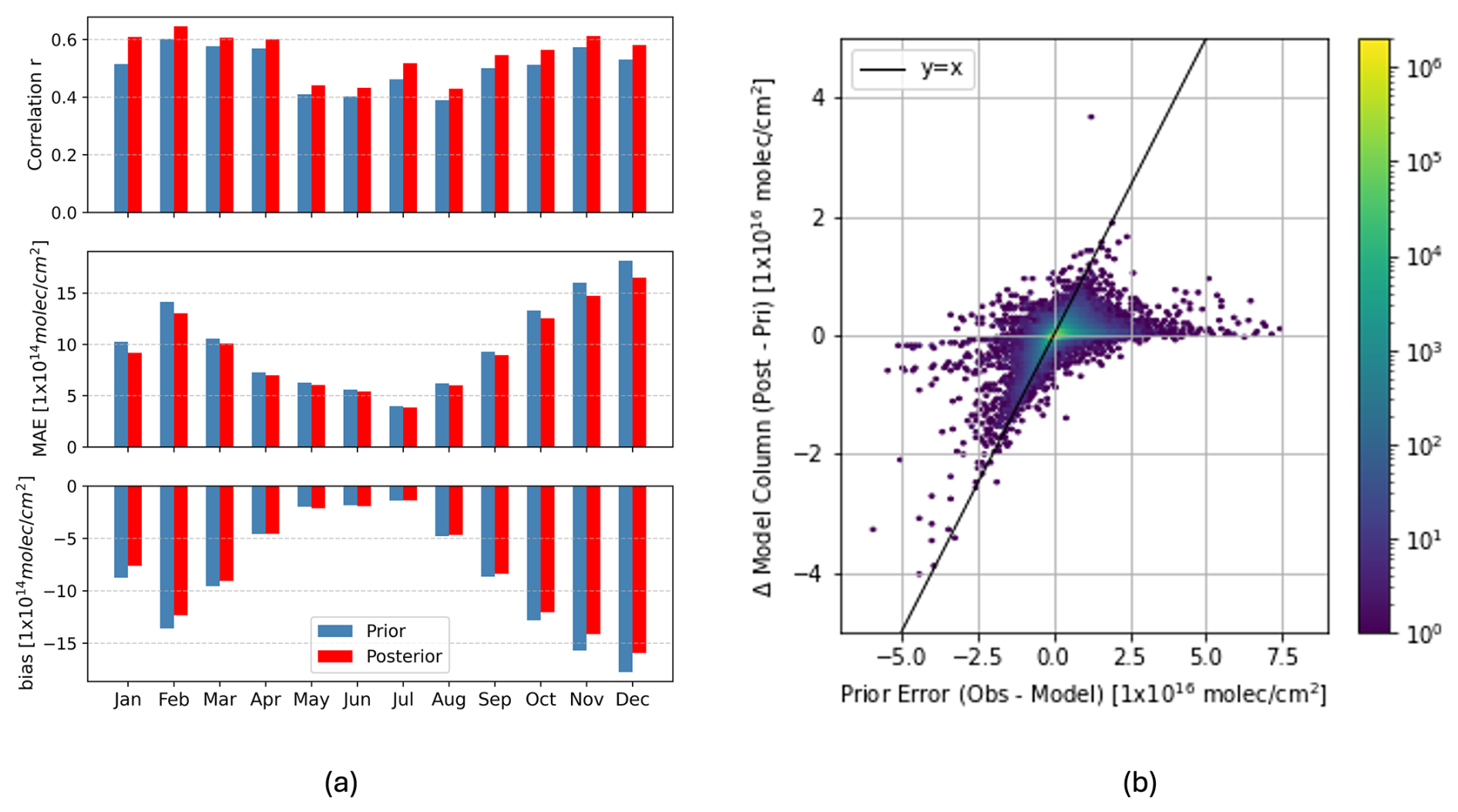
Figure 5 (a) European-wide monthly changes in model performance against TROPOMI NO₂ after posterior flux updates, shown as differences between posterior–observation and prior–observation statistics. Improvements are quantified using Pearson r, mean absolute error (MAE), and mean bias. (b) Relationship between prior model error (observation–model) and posterior adjustment (posterior–prior) at the TROPOMI retrieval level, based on all available observations aggregated over the full year (2021). Each point represents an individual observation–model comparison, with colour indicating data density.

Figure 5b shows the relationship between prior error and change in model column (posterior – prior) in TROPOMI observation space. The majority of data points are clustered around the 1:1 line, indicating that posterior adjustments scale with the magnitude and sign of the prior error and act to systematically reduce model–observation mismatch. Deviations from this behaviour, where the posterior adjustment is smaller than the prior error, are primarily associated with regions where NO₂ columns are weakly sensitive to combustion emission changes. In these cases, the signal is likely dominated by background concentrations, which are influenced by boundary and initial conditions, as well as non-combustion sources (e.g. fugitive, waste, solvent, and agricultural emissions) and biogenic processes (e.g. soil NO_x emissions), which are not directly optimised in the inversion.

Figure 6 shows the comparison of the prior and posterior ffCO₂ fluxes for Europe in 2021. We find a consistent reduction in emissions uncertainty, from a mean aggregate uncertainty of 5.6 % in the prior to 3.3 % in the posterior. For aggregated flux uncertainties, grid-level errors are combined assuming no spatial or temporal correlation by summing variances in quadrature. This, therefore should be considered a lower-bound estimate of uncertainty.

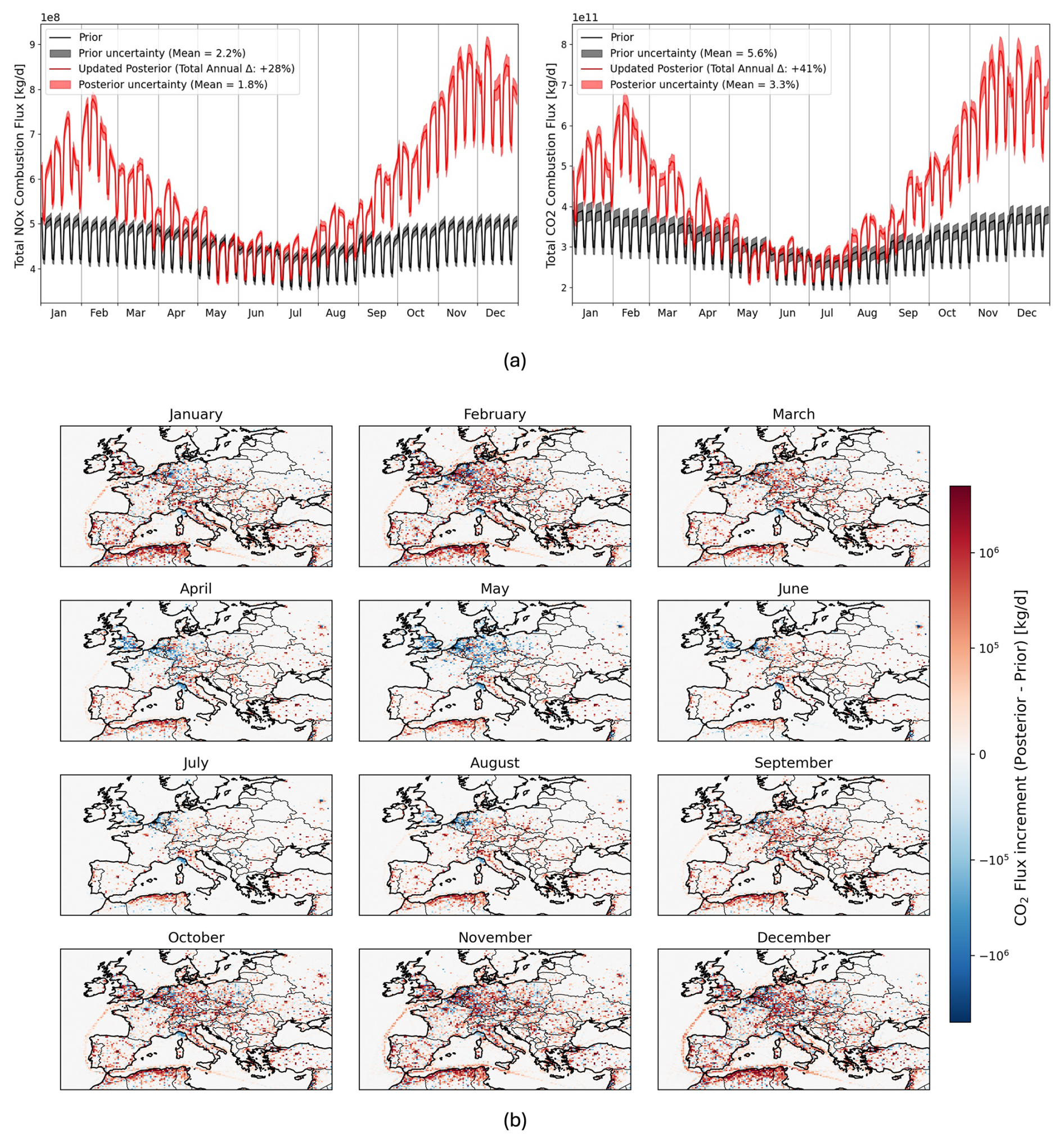
Figure 6 (a) Time series of total European daily fluxes for NO_x (left panel) and ffCO₂ (right panel) for 2021. Prior fluxes are shown in black with grey uncertainty, and posterior fluxes in red with light red shading indicating uncertainty. (b) Mean monthly posterior increment maps show the average regional trends of flux changes (red = increase, blue = decrease relative to prior).

Our European posterior ffCO₂ fluxes exhibit a more pronounced seasonal cycle than found in prior data (Fig. 6a), with larger values during autumn and winter months, most notably during February, November, and December. Conversely, fluxes between mid April and early August remain close to prior values but with a smaller uncertainty. Larger posterior adjustments during the colder months may reflect challenges in bottom-up inventories for domestic heating in winter, which are highly seasonal and subject to substantial uncertainty due to their dependence on meteorology, fuel use, and assumed temporal profiles (Denier van der Gon et al., 2015; Guevara et al., 2021; Kuenen et al., 2022).

Figure 6b shows monthly mean posterior minus prior increments across Europe. Colder months are characterised by widespread increases (10 %–177 % total European daily flux change) relative to the prior while the warmer months show a marked decrease (down to −22 % total European daily flux change), particularly over northwestern Europe (United Kingdom, Germany, Netherlands, Belgium), together with some localised increases (Spain, Italy, Turkey). It is also important to note that the interpretation of posterior flux increments should be considered in the context of spatial variations in prior uncertainty. In particular, regions such as North Africa exhibit substantially higher prior uncertainties, which allow larger adjustments but reduce the robustness of the inferred changes compared to more tightly constrained regions over Europe.

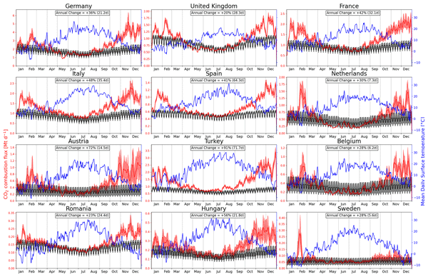
Figure 7 shows the national ffCO₂ fluxes for 12 high emitting European countries for 2021 with the corresponding mean surface temperature values derived from the GEOS-FP reanalysis. Generally, we find that individual countries follow the same pattern as the aggregated European total emission trend. Countries that show the most significant and consistent increases in emissions during the colder months include France, Spain, Italy, and Turkey. Reductions in fluxes are observed during some of the summer months in the Netherlands, Belgium, the United Kingdom, and Germany; however, these changes are generally within the range of the prior uncertainty spread.

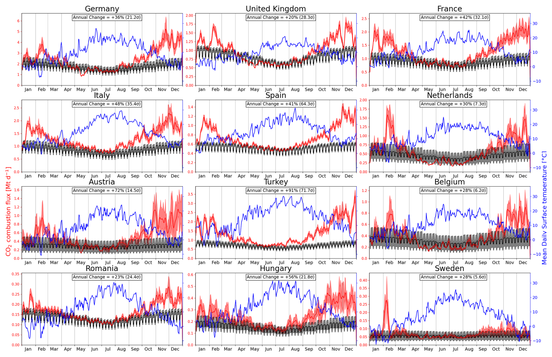
Figure 7 Time series of daily ffCO₂ emissions for 12 high emitting European countries during 2021. Prior fluxes are shown in black with grey uncertainty, and posterior fluxes in red with red shading indicating uncertainty (left y axis). Mean daily temperature is also shown in blue (right y axis). For each country, the reported annual change represents the total posterior adjustment relative to the prior, expressed both as a percentage change in annual emissions and as a multiple of the prior uncertainty (σ).

Across all countries, annual emissions increase relative to the prior, ranging from 20 % (United Kingdom) to 91 % (Turkey). The analogous national emission patterns and temperature variation for NO_x is shown in Fig. A2. The same pattern of increased correlation with temperature is prevalent with the NO_x posterior state, and emission increases are also significant but slightly smaller in size, ranging from 11 % (Sweden) to 83 % (Turkey).

We find a clear negative correlation between our ffCO₂ fluxes and local mean temperature, largely reflecting emission peaks during colder winter periods. In February, many countries experienced a considerable number of days with low temperatures, which coincided with a relative increase in emissions. This effect is most pronounced in Sweden, where the mean daily temperature stayed below −5 °C throughout the month, occasionally dropping below −10 °C, accompanied by a distinct spike in emissions compared to the rest of the year. Similar, though less extreme, cold periods were observed in Germany, the UK, the Netherlands, Belgium, and Turkey, each corresponding to relative emission peaks during February. The posterior ffCO₂ shows a strengthened temperature-flux relationship as a consistent increase in the gradient of the correlation between the two variables (Fig. A4). The prior state exhibits two distinct branches, reflecting prescribed weekday and weekend emission regimes with no variability within each category. In the posterior, these branches merge into a more continuous relationship with temperature, indicating the introduction of day-to-day variability while retaining the underlying weekly emission cycle.

At higher temperatures, increased energy demand for cooling may contribute to ffCO₂ emissions, particularly in the power sector. However, this effect is generally weaker and more regionally variable than winter heating demand in Europe, resulting in a dominant negative temperature–emission relationship. Residential heating sources (e.g. wood and coal combustion) exhibit strong seasonal variability and are more strongly reflected in NO_x than CO₂, which may lead to an amplified winter response in the inferred ffCO₂ emissions. In addition, uncertainties in NO_x : CO₂ emission ratios and the weaker NO_x signal associated with electricity-driven summer cooling (potentially supplied by low-NO_x generation) may bias the inferred temperature–emission relationship.

To provide context using an independent bottom-up benchmark, Fig. 8 compares the annual total ffCO₂ emissions for each of the 12 countries in both the prior and posterior with estimates from EDGAR. The posterior results show mixed agreement with this independent dataset. For Sweden, Romania, Turkey, Spain, and the United Kingdom, the increases in annual emissions lead to improved agreement with EDGAR. This is particularly notable for Turkey, where the large posterior increase (+91 %) leads to a substantially better agreement with the independent inventory. In contrast, the remaining seven countries show a deterioration in agreement following the posterior updates, with increases in absolute differences ranging from 25 % to over 100 % in Austria (see Table A1).

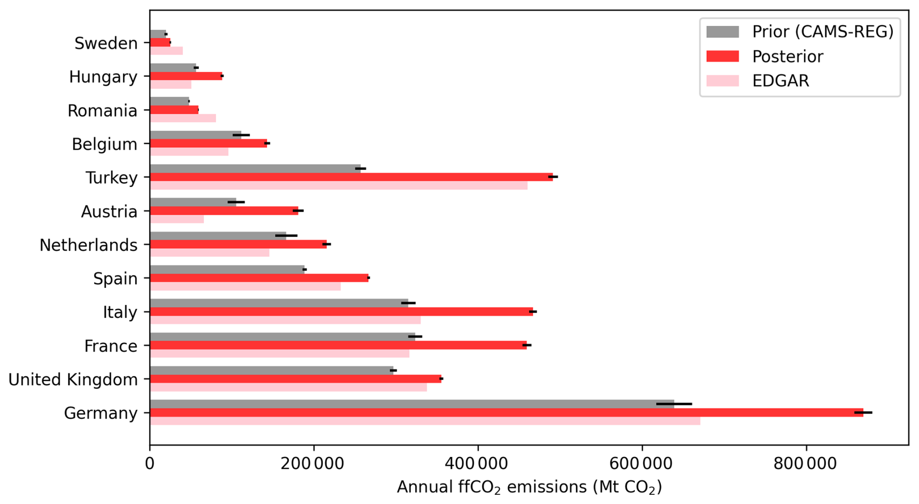
Figure 8 Annual ffCO₂ emissions by country for 2021. Comparison of prior (CAMS-REG, grey), posterior (red), and EDGAR (pink) estimates. Error bars indicate uncertainties for prior and posterior emissions. EDGAR provides an independent bottom-up benchmark.

In particular, the substantial increases inferred for Italy, France, and Germany result in pronounced overestimations relative to both CAMS-REG and EDGAR, exceeding 100 000 Mt CO₂. These discrepancies are significantly larger than the differences between bottom-up inventories, suggesting that the inferred changes in these regions could be influenced by limitations in the inversion framework rather than reflecting true emission biases.

3.2 Evaluation of the posterior solution

We evaluate our posterior emission estimates of NO_x and ffCO₂ by using the GEOS-Chem model as a forward model to calculate the associated atmospheric distributions of NO₂ and CO₂. We compare these posterior atmospheric distributions with in situ NO₂ and CO₂ measurements across Europe and with NASA OCO-2 column observations of CO₂.

Figure 9 shows the change in model agreement with the EEA in situ NO₂ monitoring network. We find a relatively strong negative bias is present in both the prior and posterior simulations (−18.8, and −16.4 µg m⁻³, respectively). Nevertheless, the posterior values show a consistent improvement in correlation, alongside reductions in both MAE and bias. On a monthly basis, MAE decreases in every month of the year, with the largest reductions occurring during the colder months when the posterior flux adjustments are greatest. Correlation improves in all months, but the improvement is most obvious in summer, where prior correlations for June and July were non-existent (r<0) in the prior.

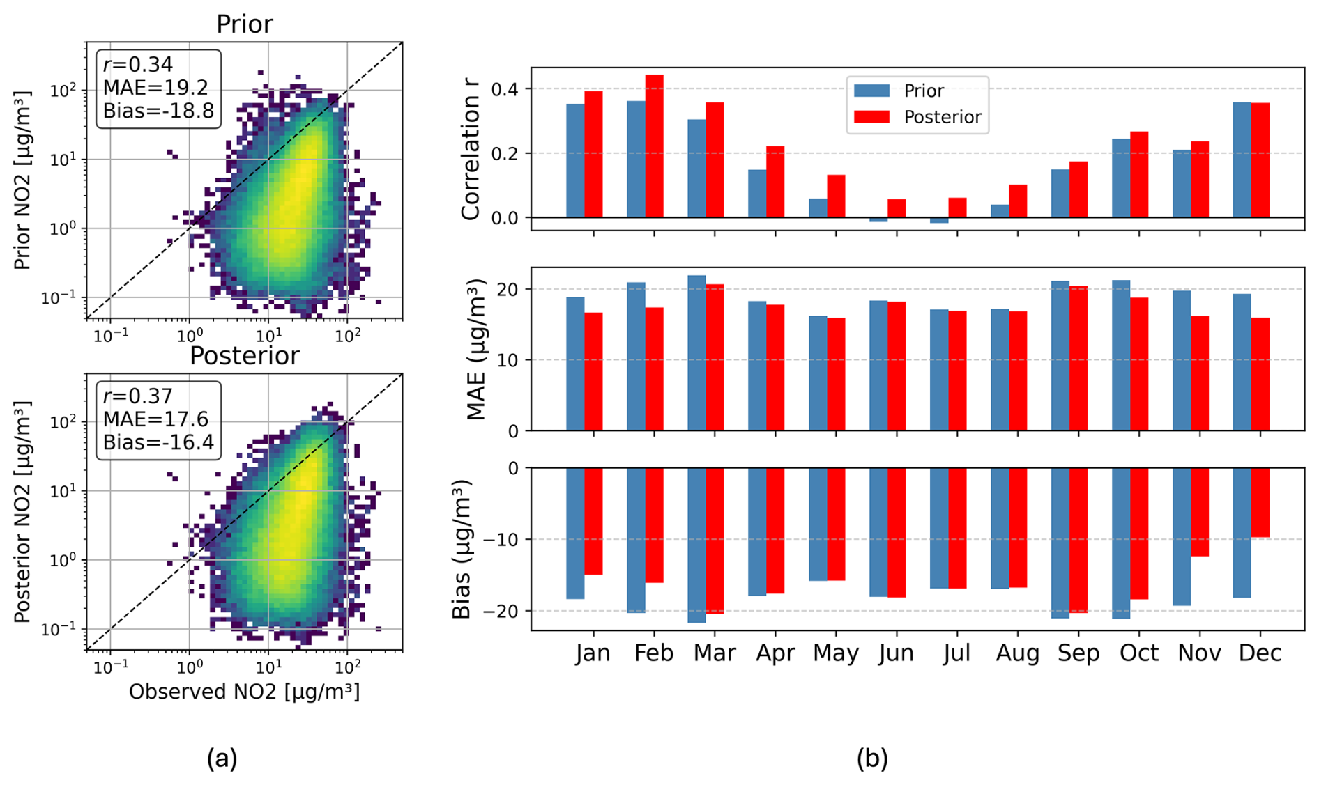
Figure 9 Model agreement with the EEA NO₂ in situ network. (a) Observed versus modelled NO₂ concentrations for prior and posterior simulations, with each point representing a model–observation pair for a given time step and station across 2021. (b) Monthly performance metrics for prior (blue) and posterior (red), computed from all model–observation pairs within each month.

The negative model bias is expected because the EEA in situ NO₂ sites are predominantly located in urban or high-combustion environments, often close to traffic and other emission sources, and therefore sample strong, localised plumes. Since NO₂ has a short chemical lifetime of hours to 1 d, this leads to strong spatial gradients and rapid decay away from emission sources. These plumes occur at spatial scales much smaller than the GEOS-Chem grid resolution (0.25°×0.3125°) and are therefore not fully resolved by the model. Instead, they are artificially diluted within the grid-box-mean representation of the lowest model layer. As a result, the model smooths sharp near-source enhancements and systematically underestimates point observations, contributing to the persistent negative bias seen in the comparisons. Overall, this consistent negative bias limits the model agreement in both the prior and posterior, and leads to relatively small performance improvement.

Figure 10 shows a similar model assessment of posterior atmospheric concentrations with in situ CO₂. Compared with prior values, the posterior CO₂ mole fraction show an overall improvement. The month-to-month comparison shows more variability than the NO₂ comparison likely due to additional uncertainties from biogenic fluxes. The correlation improves in all months except June and July. The negative bias is substantially reduced in October, November, and December, supporting the relative increases in posterior fluxes for these months. Conversely, the negative bias at these in situ sites increases in the posterior state during the warmer months (April–September), suggesting that either the posterior increment for CO₂ combustion fluxes should be larger, or that there are inaccuracies in the biogenic uptake in the SiB4 model.

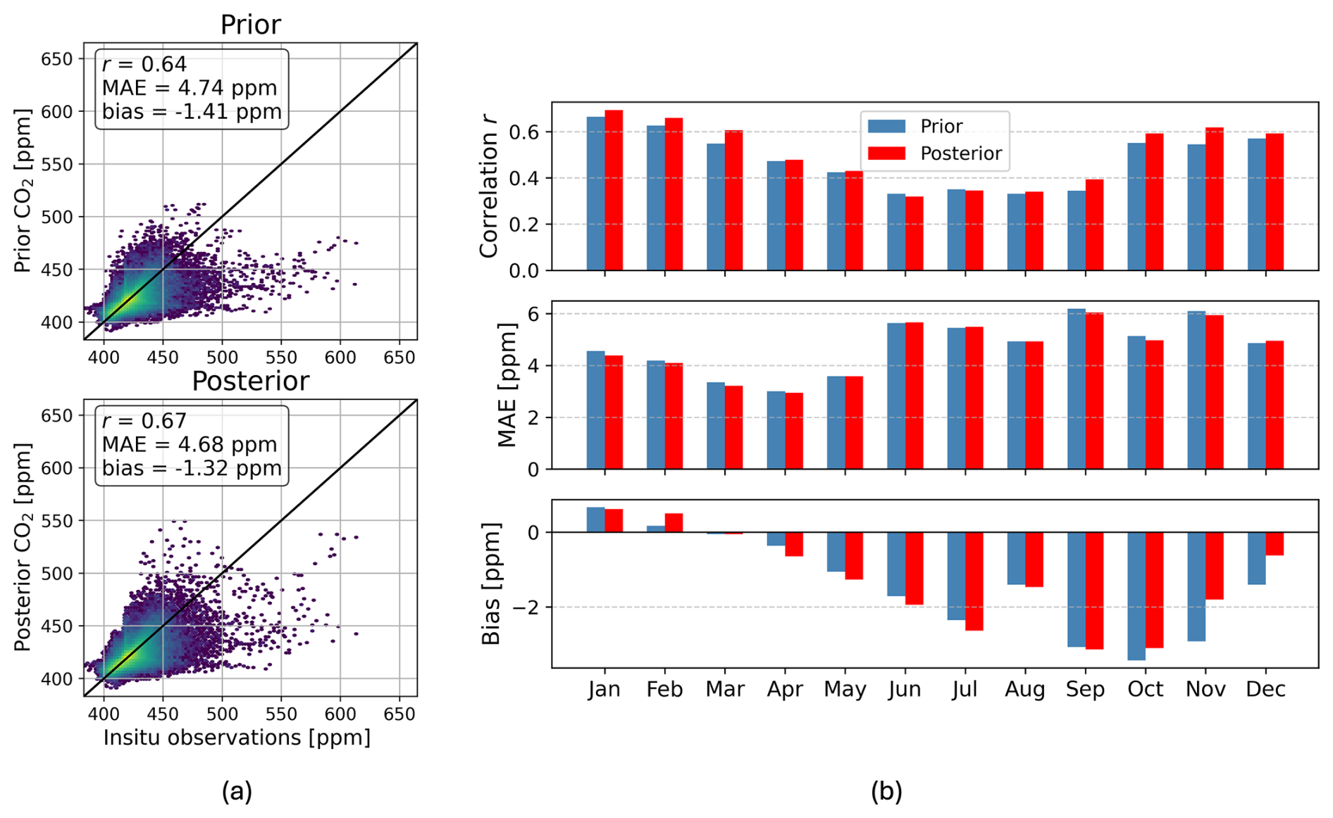
Figure 10 Model agreement with ICOS, and DECC CO₂ in situ network. (a) Observed versus modelled CO₂ concentrations for prior and posterior simulations, with each point representing a model–observation pair for a given time step and station across 2021. (b) Monthly performance metrics for prior (blue) and posterior (red), computed from all model–observation pairs within each month.

Figure 11 shows the change in model–observation MAE from prior to posterior at individual stations for each season. The improvement in agreement with the in situ NO₂ network is widespread. Almost all sites show improved agreement across all seasons, with only a small number exhibiting degradation in summer. The largest improvements are observed in winter and autumn. A slight deterioration is observed at nine sites across Northern Europe (Belgium, the Netherlands, Germany, Sweden, and Norway) and at one site in northern Spain, accounting for less than 5 % of the monitoring network. All remaining sites exhibit smaller but consistently positive improvements during the summer period. In contrast, the CO₂ in situ comparison shows substantially greater spatial variability. Approximately 50 % of sites show improvement in summer, increasing to 55 % in winter, 65 % in spring, and 77 % in autumn. Only one site (Järvselja, Estonia) exhibits a consistent degradation across all four seasons; this is a rural forest site likely strongly influenced by local biogenic fluxes. Conversely, nine sites show consistent improvement in all seasons, including four in Germany, two in France, and one each in the United Kingdom (Shetland), Italy, and Poland.

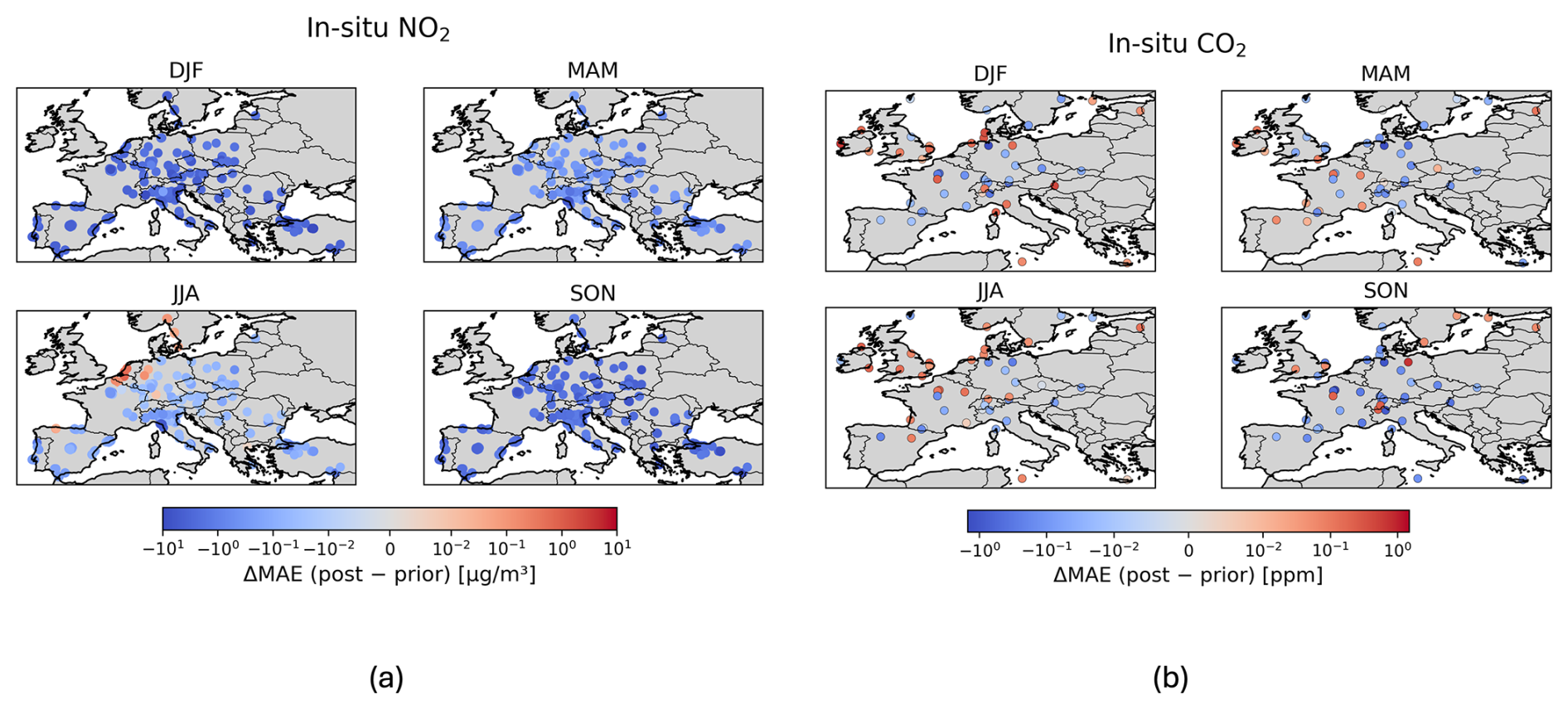
Figure 11 Seasonal changes in model–observation agreement at in situ sites for (a) NO₂ and (b) CO₂. Each panel shows one season (DJF, MAM, JJA, SON). Colours indicate the change in mean absolute error (ΔMAE = posterior − prior) at each station, computed from all model–observation pairs within each season. Negative values (blue) indicate improved agreement, while positive values (red) indicate degradation.

The majority of the CO₂ monitoring sites used here are classified as rural background or elevated stations, designed to sample regionally representative air masses. As a result, these sites are less sensitive to localised fossil fuel emission plumes compared to the predominantly urban EEA NO₂ network. This reduced sensitivity, combined with the strong influence of biogenic fluxes on atmospheric CO₂, likely explains the mixed response in posterior agreement change.

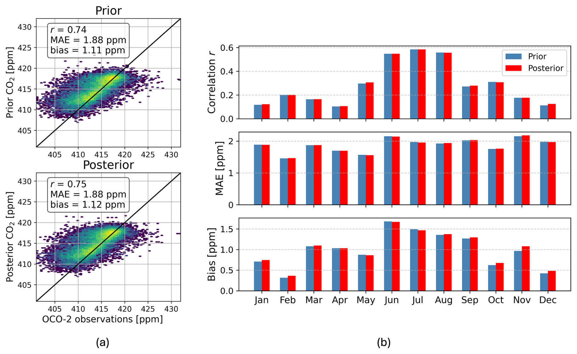
Figure 12 Model agreement with OCO-2. (a) Observed versus modelled CO₂ concentrations for prior and posterior simulations, where each point represents a model–observation pair at a given time step and station. (b) Monthly performance metrics for prior (blue) and posterior (red), computed from all model–observation pairs within each month.

Finally, we assess the posterior comparison with OCO-2 data (Fig. 12). Overall, this shows negligible improvement compared with the prior data. The shifts in correlation and error are an order of magnitude smaller than those seen in the in situ data. This is expected as column CO₂ observations are much less sensitive to surface emission changes, with variability dominated by large-scale biogenic fluxes that mask the comparatively small contribution from localised ffCO₂ emissions.

Overall, we see a marginal improvement in agreement with the annual data, with the correlation increasing slightly from 0.74 to 0.75. OCO-2 exhibits a positive bias, which is slightly reduced in June and July but worsens in the autumn and winter. Month-to-month correlations show small improvements (Δr>0.01) in January, May, September, and December, and negligible changes in remaining months ($\left|\mathrm{\Delta }r\right|<\mathrm{0.003}$).These seasonal biases are likely driven primarily by uncertainties in biogenic fluxes, as well as boundary and initial conditions, rather than changes in fossil fuel emissions. This highlights the intrinsic difficulty of constraining fossil fuel CO₂ emissions using column CO₂ observations alone.

In addition, the positive bias seen in OCO-2 comparisons contrasts with the negative bias found in surface in situ measurements, reflecting the differing sensitivities of these observing systems. Column-averaged CO₂ observations are strongly influenced by large-scale transport and boundary conditions, which can introduce a positive bias if background concentrations are overestimated. In contrast, near-surface observations are more sensitive to local fluxes and boundary layer processes, and the relatively coarse vertical resolution of the model can introduce a negative bias when comparing modelled near-surface concentrations with point measurements. These differences highlight the challenges in reconciling column and surface constraints within a single inversion framework.

Overall, the posterior results demonstrate measurable improvements in model–observation agreement with independent datasets, alongside a strengthened relationship between emissions and temperature, and an improved agreement with EDGAR for a subset of countries. At the same time, the inferred emission changes are substantial, with all national annual adjustments exceeding the magnitude of the prior uncertainty by factors of approximately 6 (Sweden, Belgium) to 70 (Turkey). These adjustments likely reflect a combination of prior inventory biases and structural assumptions within the inversion framework. A more detailed discussion of these assumptions and their implications is provided in the concluding remarks.

4 Concluding remarks

We have presented a satellite-driven ensemble data assimilation framework that utilises TROPOMI NO₂ observations to constrain European NO_x flux estimates and provide an indirect estimate of ffCO₂ emissions for 2021. By implementing a reduced-complexity NO_x chemistry module within GEOS-Chem, we achieved a computationally efficient pathway for inversion runs that retains critical chemical feedbacks. This approach reduced posterior flux uncertainty by around 40 % (from 5.6 % to 3.3 %).

Our results reveal a pronounced amplification of the ffCO₂ seasonal cycle – driven by enhanced emissions in autumn and winter – that correlates strongly with surface temperature variability. While independent validation against in situ measurements confirms improved model performance, the limited sensitivity of OCO-2 comparisons highlights the ongoing challenge of isolating fossil fuel signals from large biogenic backgrounds. Ultimately, this study demonstrates that NO₂-driven assimilation can provide a first-order constraint on anthropogenic emissions.

We acknowledge that our posterior flux adjustments imply substantial increases in national ffCO₂ emissions relative to the prior inventory. For all analysed countries the annual total increases by more than 20 %, with the largest changes reaching up to 91 % in Turkey. These values exceed the stated prior uncertainty and therefore warrant careful interpretation. These results should be interpreted in the context of the limitations of the inversion framework. A key limitation is the use of prescribed, temporally invariant NO_x : CO₂ emission ratios. In practice, NO_x : CO₂ emission factors vary across sectors, regions, and seasons due to differences in combustion conditions, fuel composition, and technology (Jiang et al., 2010; Wang et al., 2025; Super et al., 2020a). The lack of temporal variability in these emission factors, together with any errors in the assumed prior emission relationship, may introduce systematic biases in the inferred CO₂ flux adjustments.

In addition, non-combustion and biogenic NO_x sources are held fixed at their prior values. In particular, soil NO_x emissions represent a highly variable and uncertain source during summer, driven by meteorological and agricultural factors, and remain an active area of research (Vinken et al., 2014; Lin et al., 2024). As a result, uncertainties in these sources cannot be directly corrected and may instead be compensated for through adjustments to combustion emissions. Furthermore, the reliance on a single daily satellite overpass requires prescribed diurnal emission profiles, and the use of a 1 d assimilation window limits the representation of temporal variability in emission uncertainties. These limitations underscore the need for additional constraints, which we propose to address in future work. This study should therefore be viewed as a proof-of-concept inversion approach, and the results should be interpreted as an initial estimate rather than a definitive correction to national emission inventories.

A range of complementary approaches have recently emerged for inferring ffO₂ emissions from satellite observations, including direct plume detection methods, machine learning-based frameworks, and observed cross-tracer ratio techniques. Plume detection approaches exploit high-resolution CO₂ imagery to quantify point-source emissions (Hakkarainen et al., 2016; Kuhlmann et al., 2020; Cusworth et al., 2021), but are generally limited to large, isolated emitters and favourable atmospheric conditions. Machine learning methods offer computational efficiency and the ability to capture complex nonlinear relationships in atmospheric data (Ji et al., 2024; Zheng et al., 2026), although they typically rely on large, representative training datasets and may lack physical interpretability. Cross-tracer approaches leveraging combined NO₂ and CO₂ analysis, provide a promising framework for improving source attribution and reducing ambiguity in ffCO₂ signals (Reuter et al., 2019; Yi et al., 2026).

The approach presented here lies within this emerging class of multi-species top-down methods, building on earlier studies combining NO₂ and CO₂ observations to improve constraints on combustion emissions (Kuhlmann et al., 2021; Kaminski et al., 2022; Santaren et al., 2025). Assimilating NO₂ observations benefits from the high sensitivity of the short-lived tracer to combustion sources, enabling stronger constraints on the spatial and temporal variability of emissions. As such, this framework provides a physically consistent pathway for exploiting reactive trace gas observations, and should be viewed as complementary to existing methodologies. At the same time, it highlights the importance of developing integrated, multi-species inversion frameworks to further improve separation of fossil and biogenic flux components.

Looking forward, the transition toward high-resolution, multi-species satellite constellations necessitates a shift in how we process reactive gas chemistry within carbon-cycle inversions. The success of our reduced-complexity NO_x framework suggests that the historical trade-off between chemical accuracy and computational feasibility is less likely to be a barrier to future operational monitoring. As the Copernicus CO2M mission and GOSAT-GW begin to provide co-located CO₂ and NO₂ retrievals at high spatial and temporal resolution, and geostationary platforms such as TEMPO offer enhanced constraints on the diurnal variability of NO₂, this ensemble-driven approach has the potential to be scaled to provide near-real-time quantification of anthropogenic emissions.

A key next step is the development of a fully coupled NO₂–CO₂ inversion framework, in which both species are assimilated simultaneously, allowing emission ratios to be dynamically constrained and improving the separation of fossil fuel and biogenic flux components. Ultimately, these advancements will move the community closer to a transparent, satellite-based verification system capable of supporting international climate accords and sub-national emission reduction targets.

Appendix A

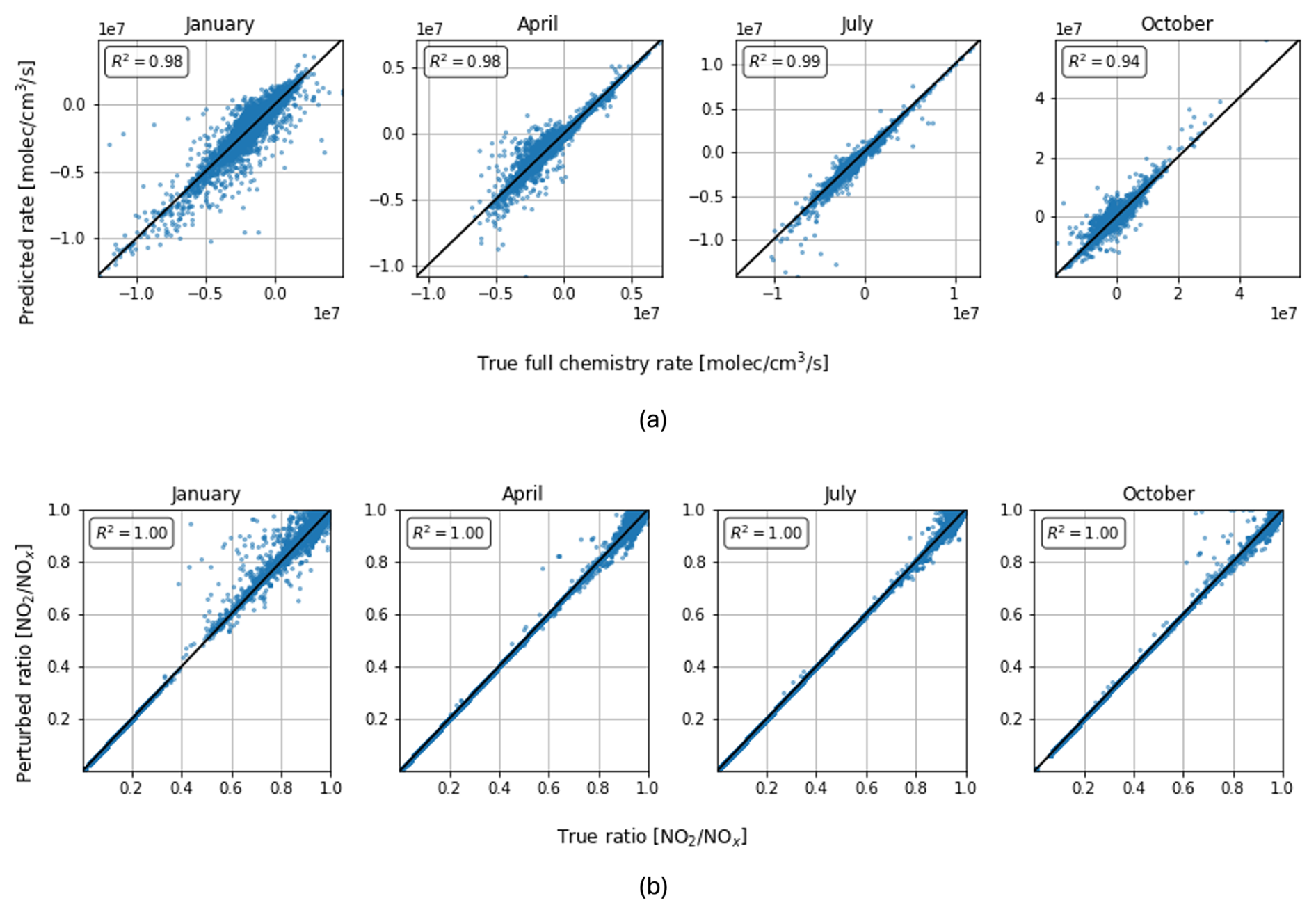
Figure A1 Evaluation of the offline NO_x chemistry parameterisation against full GEOS-Chem chemistry for emission perturbations representative of the posterior solution. Panel (a) shows the comparison between “true” NO_x chemical loss rates (from the full chemistry simulation) and those predicted by the offline linear scaling scheme. Panel (b) shows the corresponding comparison for the NO₂ : NO_x partitioning ratio. In both cases, results are shown for a single representative day in each season (January, April, July, and October), using emission perturbations consistent with the posterior increments. High agreement (R² between 0.94 and 0.99) in panel (a) demonstrates that the offline scheme accurately reproduces nonlinear chemical responses under large perturbations, while the near-perfect agreement in panel (b) indicates that the NO₂ : NO_x partitioning remains largely unchanged. Together, these results confirm the validity of the offline chemistry approximation and the assumption of stable partitioning across the range of emission perturbations explored in this study.

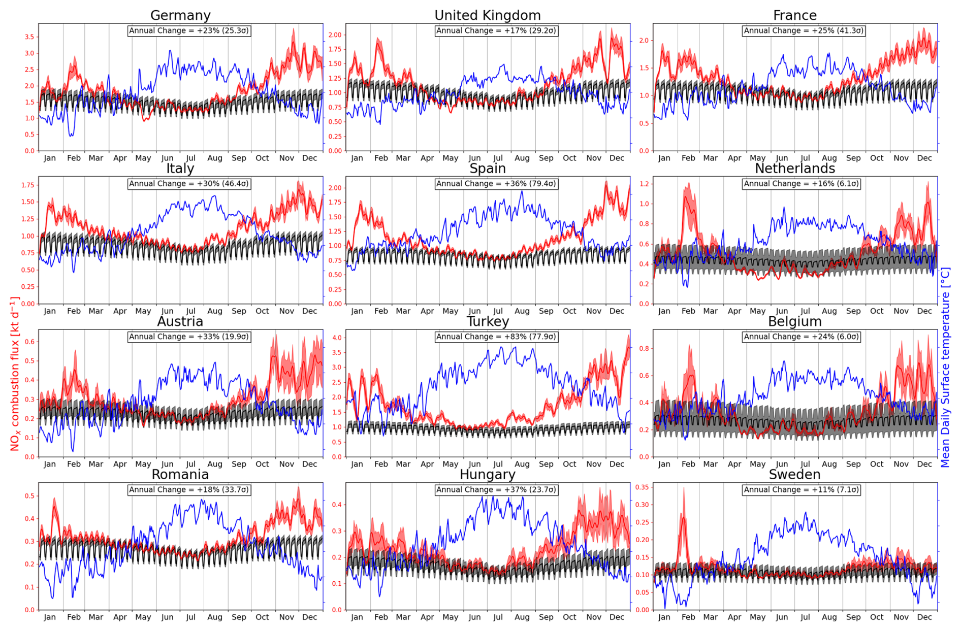
Figure A2 Full year NO_x combustion emissions for 12 high emitting European countries. Prior fluxes are shown in black with grey uncertainty, and posterior fluxes in red with red shading indicating uncertainty (left y axis). Mean daily temperature is also shown in blue (right y axis).

Table A1 Comparison of prior and posterior ffCO₂ emissions relative to EDGAR for selected European countries. Differences are shown in absolute terms (Mt CO₂) and as percentage changes in agreement relative to EDGAR. Positive values of improvement indicate reduced disagreement.

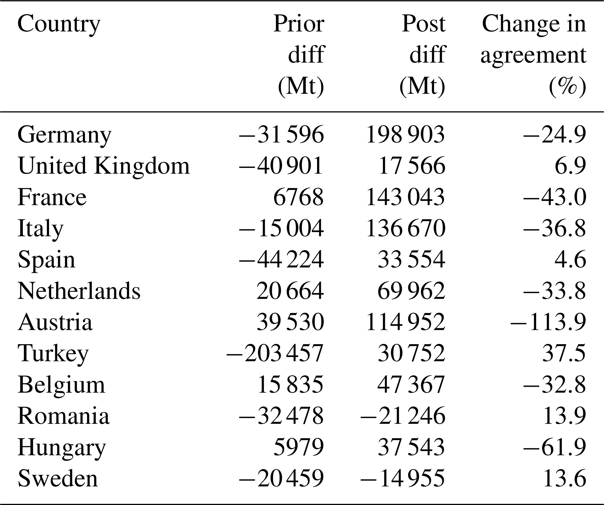
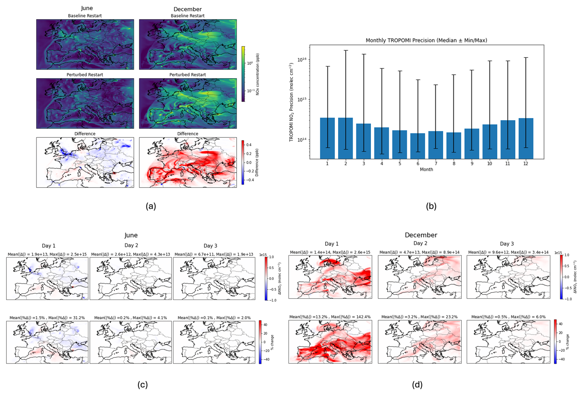
Figure A3 Assessment of modelled XNO₂ column sensitivity to changes in the restart file. (a) Two examples comparing the baseline and perturbed restart files. The June example shows a general decrease in NO_x concentrations in the perturbed state, with small localised increases in the south, whereas the December example shows widespread increases across most of the region. (b) Median and range of TROPOMI precision for each month of 2021. (c, d) Column difference, ΔXNO₂ (molec. cm⁻²) and relative differences (%) between simulations using the two restart files, shown for June (c) and December (d) over days 1, 2, and 3 of the model run. By day 2 in June, the maximum absolute column differences are below TROPOMI precision. In December, by day 2, the mean absolute difference is below, and the maximum absolute difference is comparable to, TROPOMI precision. These results indicate that restart file deviations primarily affect XNO₂ on the first day of the model run, with subsequent days showing changes within or below TROPOMI precision limits.

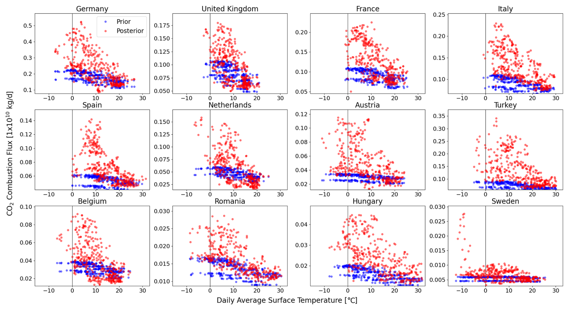
Figure A4 Scatter plots showing the daily average surface temperature against CO₂ combustion fluxes for 12 high emitting countries. The prior fluxes are shown in blue, and the posterior fluxes in red.