The Cold-Air Outbreaks in the Marine Boundary Layer Experiment model-observation intercomparison project (COMBLE-MIP) – Part 1: Model specification, observational constraints, and preliminary findings

Models struggle to represent the coupled microphysical, turbulent and radiative processes within widespread, long-lived marine cold-air outbreak (CAO) cloud fields, contributing to forecast and climate biases. Here we combine ground-based and satellite measurements to initialize and constrain large-eddy simulations (LES) of cloud field evolution with distance downwind from the marginal ice zone during a strong, highly supercooled and convective CAO observed during the Cold-Air Outbreaks in the Marine Boundary Layer Experiment (COMBLE). LES results are compared with large-scale models run in single-column model (SCM) mode, providing an observation-constrained framework for large-scale model evaluation and future improvements. All models reproduce rapid cloud formation off the ice edge, and a monotonic ascent of downwind cloud-top heights, closely linked with time-integrated surface heat fluxes. LES generally reproduce domain-mean observational targets using a modest test domain (25×25 km²), and a larger domain (125×125 km²) enables better reproducing the observed growth of convective cell sizes. In realistic mixed-phase LES compared with liquid-only simulations, ice processes lead to thinner, broken cloud decks and substantially reduced cloud radiative effects on top-of-atmosphere longwave fluxes. By contrast, mixed-phase SCM simulations generally underpredict the radiative impact of ice, primarily owing to insufficient reduction of cloud cover. Results indicate that cellular cloud structure is qualitatively captured by LES, and thus LES could provide guidance to improvement of large-scale model physics schemes. Follow-on work will extend these results to larger domains, apply objective analysis of mesoscale structure, and include prognostic aerosol properties for droplet and heterogeneous ice formation.

1 Introduction

The Arctic has been warming 3–4 times faster than the rest of the globe in recent decades (Rantanen et al., 2022), more rapidly than Earth system models (ESMs) have predicted (Johannessen et al., 2016; Serreze et al., 2009; Wuebbles et al., 2017; Taylor et al., 2022). Thus, coupled climate system feedbacks are more pronounced regionally, with positive feedbacks exacerbating the global warming trend. One of the leading yet poorly understood feedback mechanisms contributing to this Arctic amplification involves clouds (Middlemas et al., 2020), with changes in cloud phase and vertical structure in a warmer Arctic troposphere and reduced sea ice cover likely enhancing warming to an uncertain degree (Kay et al., 2016).

During the winter and spring months in the Northern Hemisphere, poleward warm air intrusion events and opposing cold-air outbreak (CAO) events sweep through the Arctic and sub-Arctic (Pithan et al., 2018), e.g. at 70° latitude the meridional atmospheric latent and sensible heat transfer is about 65 % larger in the Northern than the Southern Hemisphere (Trenberth and Caron, 2001). The balance (or lack thereof) between these two contrasting synoptic flow regimes ultimately controls the winter- and springtime radiative and moisture budgets in the region (Lackner et al., 2023a; Pithan et al., 2018). During CAOs, air masses advect from relatively cold environments (e.g., landmasses or sea ice) to the relatively warm open ocean, leading to intense air-sea exchanges and convectively-driven motions (Fletcher et al., 2016a, b). These conditions typically produce mixed-phase clouds, containing both supercooled liquid and solid (ice) phase hydrometeors (e.g., Korolev and Milbrandt, 2022). CAO mixed-phase clouds are characterized by pronounced mesoscale structures evident in satellite imagery, associated with continuous microphysical and radiative evolution as air masses transit over the open ocean (Xia and McFarquhar, 2024). While numerical weather prediction (NWP) and ESMs may skillfully predict the relatively long-lived, large-scale meteorological patterns typically associated with CAOs (e.g., Polkova et al., 2021), models are universally challenged to represent the coupling of buoyancy- and shear-driven turbulence, mixed-phase aerosol-cloud-precipitation interactions, and complex mesoscale structures that are generally considered to be driven by convective cold pools and cloud-top radiative cooling. It is these CAO conditions that will be the focus of this multi-part study.

Over Arctic pack ice under initially clear-sky conditions, the stable or nearly neutral atmospheric boundary layer (BL) is generally relatively shallow, with an ice-breeze jet typically present near a strong inversion layer (e.g., Chechin et al., 2013). Further south (downwind) over the marginal ice zone (MIZ), where there are patches of both open ocean and ice, a fairly rapid change in surface forcing occurs. Reaching first open leads and then open water, the skin temperature (TSK) is much higher (by as much as ∼25 °K) than that of the ice, leading to some of the largest total surface turbulent heat fluxes observed on Earth (Papritz et al., 2015; Fletcher et al., 2016b; Aemisegger and Papritz, 2018). In response, the BL rapidly deepens through vertical turbulent mixing, constrained by the free-tropospheric (FT) stability and subsidence, while gaining heat and moisture. Here a thermal wind, induced by horizontal temperature gradients associated with a rapidly increasing BL depth, may increase or decrease horizontal wind speeds locally, depending on the angle of the ice edge relative to the geostrophic wind direction (e.g., Chechin et al., 2013; Chechin and Lüpkes, 2017). Chylik (2017) showed that the influence of surface heterogeneities in the MIZ depends on wind shear, the size and orientation of the heterogeneity, and the initial stratification. Discontinuities in ice edge orientation may also lead to persistent rift structures or convergent cloud bands that extend far downwind (Spensberger and Spengler, 2021). Sufficient mixing and fetch generally lead to a more or less overcast cloud field, with shallow convective cloud structures usually organized as quasi-linear rolls within a BL subject to strong wind shear and large surface heat fluxes. As marine BL (MBL) air continues to advect downstream over open water, the continued turbulent transfer of heat and moisture from the ocean into the atmosphere leads to further deepening of the BL and widening of the roll structures (e.g., Young et al., 2002). However, the relationship between the roll aspect ratio (defined as the cloud street spacing relative to the MBL depth) and MBL depth is not well understood (e.g., Kristovich et al., 2003; Wu and Ovchinnikov, 2022). The relative contributions of potential mechanisms promoting roll formation and maintenance also remain unclear (e.g., Young et al., 2002).

At greater distance downwind, organized rolls commonly transition into closed cellular structures in a manner that may be abrupt or more smoothly continuous. During this transition, the wind shear and heat fluxes decrease (e.g., Khanna and Brasseur, 1998; Liu et al., 2006), while precipitation processes tend to become more active. With sufficient fetch, closed cells may become relatively large open cells, sometimes referred to as MBL convective complexes, where cold pool dynamics may become important in the evolution of cloud macrostructure (e.g., Zheng and Miller, 2022). Recent studies indicate the importance of phase-partitioning (liquid- and ice-phase) of the precipitation, which impacts sublimation and cold pool strength, in decoupling the MBL, breaking up the cloud deck, and promoting open cells (e.g., Egerer et al., 2023; Juliano et al., 2024; Tornow et al., 2021, 2023; Wu et al., 2025). Thus, predicting the downwind locations and rates of such morphological transitions may be sensitive to how well a model represents aerosol and cloud physics, as well as BL dynamics. In general, the impact of surface heterogeneities on mesoscale organization appears to diminish with distance from the MIZ (Gryschka et al., 2014). In summary, the importance of first-order physical processes responsible for the development of long-lived rolls and their transition to cells remain poorly established, at least in part explaining a lack of reliable model skill.

Despite their prevalence, our understanding of marine CAO cloud properties, their role in energy and water cycles, and their representation in climate models is arguably among the poorest of all cloud types (Rémillard and Tselioudis, 2015). It is well known that NWP models have difficulty representing various aspects of cloud microphysical processes, which are tied to macrostructure and turbulence (e.g., Field et al., 2017; Forbes and Ahlgrimm, 2014). A main NWP modeling inadequacy relates to mesoscale cloud organization. For instance, the MBL is relatively shallow (∼100s of meters to ∼1 km) near the ice edge where roll structures commonly initiate. Relatively high-resolution mesoscale NWP simulations with horizontal grid cell spacing, Δ, ∼1 km will not properly resolve roll structures (e.g., Tomassini et al., 2017) due to “Terra Incognita” (Wyngaard, 2004) considerations. A recent study shows that even cellular clouds, which are much larger convective CAO structures, are represented very differently by different planetary boundary layer parameterizations in high-resolution mesoscale simulations (Juliano et al., 2024). Therefore, an LES approach is required to properly represent the scales of atmospheric motion that are relevant in this regime. One LES challenge is that accurate atmospheric initialization and forcing is important to generate realistic LES results, a challenge that can be overcome by using detailed in-situ measurements, such as from aircraft dropsondes and probes (e.g., Tornow et al., 2025).

ESMs face similar challenges in simulating sub-Arctic CAO conditions (e.g., Tselioudis et al., 2021). Focusing on the realism of basic CAO properties (vertical structure and radiative transfer), in comparison to observations and well-constrained LES as a function of atmospheric thermodynamic and aerosol states, offers one pathway forward to evaluate and improve ESM cloud physics in general. Efforts have been made to identify differences in ESM physics parameterizations that are most responsible for differing predicted equilibrium climate sensitivity (ECS) values, pinpointing differing shallow cloud responses to warming as a key driver of ECS range, including both warm and mixed-phase clouds, such as CAOs (e.g., Zelinka et al., 2020). McCoy et al. (2020) also showed that precipitation processes at mid- and high-latitudes, and specifically the rate at which moisture is depleted by precipitation processes, is critical to determine extratropical cloud feedbacks. These feedbacks may be the dominant determinant of the ECS spread in CMIP6 models (Zelinka et al., 2020). McCoy et al. (2020) and Mülmenstädt et al. (2020) advocate testing the parameterization of mixed-phase and aerosol-modulated processes impacting precipitation as a key avenue for reducing uncertainty in predicted extratropical shortwave cloud feedbacks and ECS. Owing to the knowledge gaps remaining in basic physical processes, such as primary and secondary ice formation as one prominent example (Morrison et al., 2020), a strong observational foundation is needed to focus on process realism.

Even though mixed-phase clouds are omnipresent during high-latitude marine CAOs, the dominant connections between large-scale subsidence, radiation, vertical wind shear, turbulence, air-sea interactions, BL circulations, aerosol properties, precipitation, and cloud roll and cellular structural evolution remain unclear. For example, Young et al. (2018a) found that increasing subsidence, which can be substantial in CAOs (Paulus et al., 2024), leads to a more coupled and dynamic MBL due to increased liquid water path (LWP), efficient longwave (LW) radiative cooling, and more rain evaporating and snow growing below cloud. Moreover, when radiation and surface evaporation are not able to sufficiently cool and moisten the BL, strong, large-scale subsidence events can collapse Arctic mixed-phase clouds (Neggers et al., 2019). Which structural aspects of CAOs are most important to represent well in large-scale models also remains unclear. For example, based on a denial-of-mechanism LES study where MIZ surface heterogeneity was required to trigger roll initiation, Gryschka et al. (2014) found that MBL net fluxes were not strongly affected by the rolls and therefore concluded that rolls are not crucial to parameterize in large-scale models; this may not apply to the open cellular cloud regime, where Synthetic Aperture Radar imagery indicates large variations in wind speed. Here we focus on a CAO case study that is distinguished by intense supercooling and rapid MBL deepening. Emphasis is placed on the coupling of dynamical, microphysical, and radiative processes, using a stepwise approach to increasing realism (complexity) in the representation of aerosol-modulated droplet and ice formation.

Several prior community model intercomparison projects (MIPs) have sought to better understand Arctic mixed-phase clouds and their representation by LES, NWP, and climate models. Such efforts have included LES of meteorologically diverse case studies observed during the Mixed‐Phase Arctic Cloud Experiment (M-PACE; Klein et al., 2009; Morrison et al., 2009a), the Surface Heat Budget of the Arctic Ocean (SHEBA) campaign (Morrison et al., 2011), the Indirect and Semi-Direct Aerosol Campaign (ISDAC; Ovchinnikov et al., 2014), the Arctic Summer Cloud and Ocean Study (ASCOS; Stevens et al., 2018), and the Cold Cloud Microphysical Parameterisation Studies project (CONSTRAIN; de Roode et al., 2019). Of these, Klein et al. (2009) and de Roode et al. (2019) simulated CAO conditions similar to those studied here; we refer to Krueger et al. (2016) for a discussion of several earlier Arctic MIPs. Whereas Klein et al. (2009) focused on comparing LES and ESMs in single-column model (SCM) mode, de Roode et al. (2019) focused on the performance of models from LES through NWP grey zone resolutions, as discussed further below.

This MIP work focuses on the most intense CAO that was observed during the U.S. Department of Energy (DOE) Atmospheric Radiation Measurement (ARM) user facility's Cold-Air Outbreaks in the Marine Boundary Layer Experiment (COMBLE; Geerts et al., 2022). The main objective of this COMBLE-MIP is to evaluate the capability of LES and SCM simulations to reproduce the evolution (∼1000 km distance) of Arctic convective mixed-phase cloud features under strong surface forcing and highly supercooled cloud conditions. We seek to understand the fundamental convective BL and mixed-phase cloud properties, including the spread between state-of-the-art models, as well as explore which factors control mesoscale cloud organization and cloud physical properties in simulations under the observed conditions. A specification for aerosol-aware models includes an initial aerosol profile with prescribed tri-modal size distribution and windspeed-dependent surface sea spray fluxes to incorporate the impact of evolving aerosol fields on droplet and ice formation processes. Ground-based measurements taken during COMBLE, in addition to satellite observations, are combined with various data analysis techniques to tackle the aforementioned goals. Here in Part 1 of a multi-part study, we describe the model specifications and constraining observations for simulations without interactive aerosol. We present large-domain results for only two LES, and test domain results for the remaining LES. Part 2 will use interactive aerosol for prognostic hydrometeor number concentrations.

2 COMBLE-MIP modeling approach

2.1 Summary of COMBLE and CAO event

During the COMBLE field project, the first DOE ARM Mobile Facility (AMF1) was deployed to Andenes, Norway (Fig. 1) from December 2019 through May 2020. Instrumentation included an aerosol observing system (AOS), radar wind profiler, Doppler lidar, micropulse lidar, and the Ka-band ARM zenith radar (KAZR) (Geerts et al., 2022). The main goal of COMBLE was to sample shallow convection during CAO conditions, which occurred approximately 19 % of the time during the field deployment. Findings from the COMBLE campaign have yielded key insights into the CAO cloud regime (Juliano et al., 2024; Lackner et al., 2023a, b, 2024; Mages et al., 2023; Wu and Ovchinnikov, 2022; Wu et al., 2025). Out of a total of 17 CAO events with organized CAO clouds (Lackner et al., 2024), we selected the 13 March 2020 case as the basis for COMBLE-MIP. In addition to being the strongest event during the deployment, this event was selected due to the straighter air mass trajectory (Wu and Ovchinnikov, 2019) and the occurrence of distinct cloud transitions, as well as good data availability.

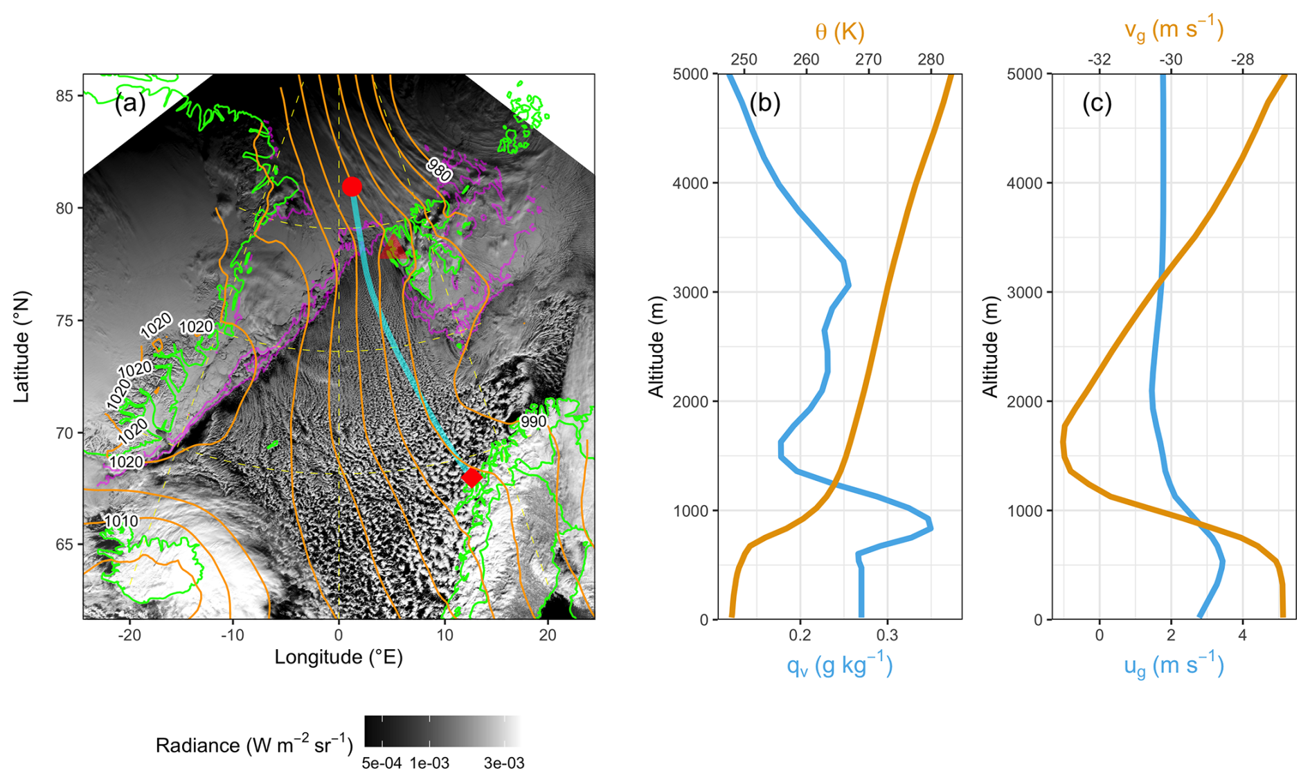
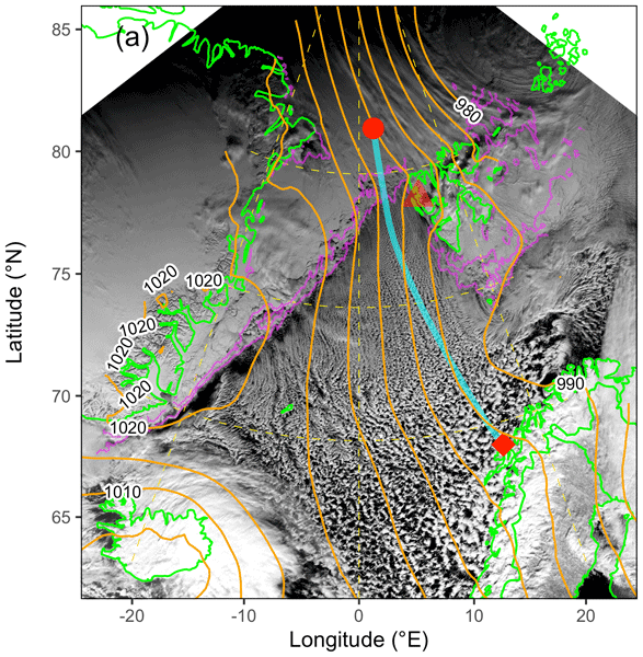
Figure 1 (a) Visible satellite imagery from VIIRS (contour filled according to colorbar, acquired at 11:18 and 11:24 UTC on 12 March 2020) overlaid with ERA-5 sea-level pressure contours (labels in hPa, from 12 March 2020, 11:00 UTC) and ASMR-E/AMSR2 sea ice edge (magenta, Melsheimer and Spreen, 2019). The trajectory path that the quasi-Lagrangian model domain follows is shown by the cyan line, starting upwind of the MIZ northwest of Svalbard (red circle) and ending at Andenes (red diamond). Initial profiles of (b) potential temperature and water vapor mixing ratio and (c) zonal (blue) and meridional geostrophic wind components. Line colors in (b) and (c) correspond to respective top and bottom x-axes.

The 13 March case was characterized by a postfrontal airmass swiftly bringing very cold air into the Fram Strait between Greenland and Svalbard. A full fetch CAO was seen in satellite imagery, with rolls transitioning to closed cells and the eventual development of open cells near the Norwegian coastline. At the AMF1 site, an open cellular lifecycle was observed (Lackner et al., 2024), with developing, mature, and dissipating cloud stages evident. In general, cloud top heights ranged from ∼3–5 km (cloud top temperatures approaching −40 °C), and pockets of high LWP occurred in the presence of strong vertical motion and enhanced turbulence. Cold pools were produced as a result of intense precipitation (Lackner et al., 2024; Juliano et al., 2024), typically in the form of snow or graupel (Mages et al., 2023).

2.2 Case specification

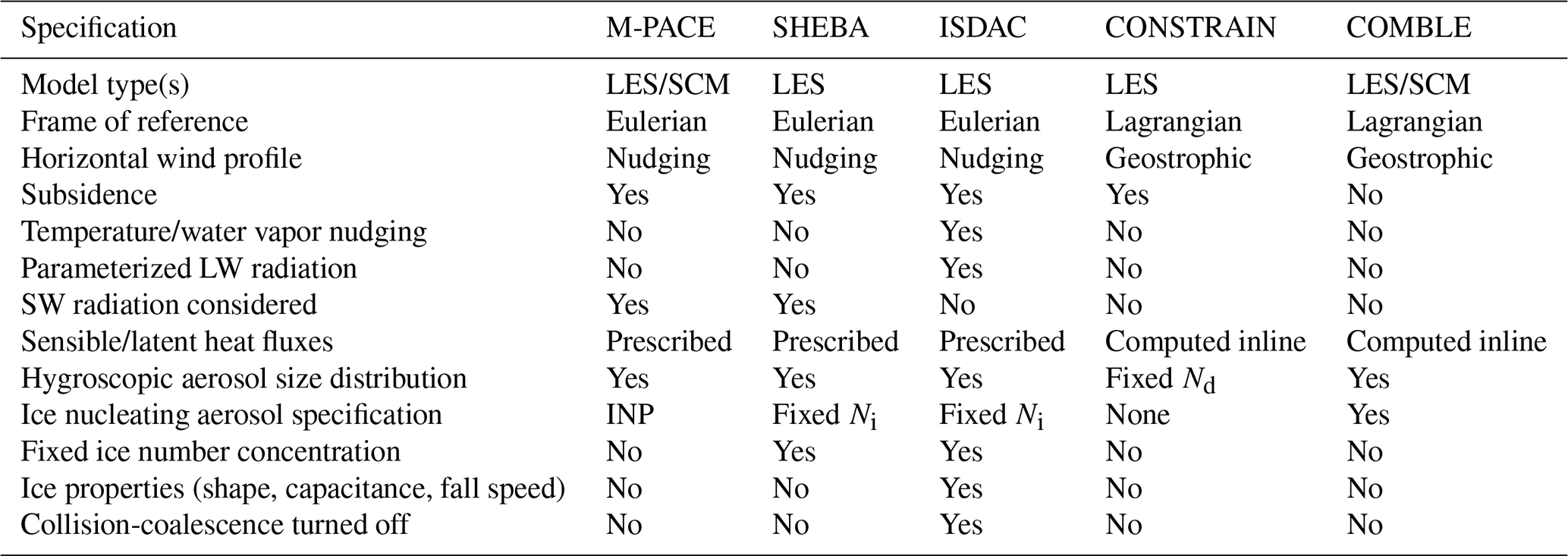
A summary of the COMBLE-MIP specification, as compared to previous Arctic MIPs, is shown in Table 1. The text in this section describes our choices in greater detail. Sensitivity simulations conducted to arrive at the final specification are outlined in Appendix A, B, and C.

Table 1 Case study setup: COMBLE-MIP compared to previous Arctic MIPs.

2.2.1 Frame of reference, initial conditions, and domain setup

The COMBLE-MIP framework uses a quasi-Lagrangian domain to simulate the formation and evolution of CAO clouds from upwind of the MIZ to the AMF1 observation site at Andenes (Fig. 1) within a modest LES domain (25×25 km²), which substantially reduces computational demand compared with a stationary domain encompassing the full trajecory length. This approach was proven to be quite useful to examine CAO cloud evolution during the CONSTRAIN MIP (de Roode et al., 2019). Moreover, such a setup is suitable for participation of both LES and SCM models (much like the M-PACE MIP), enabling a connection between models that can resolve small scale cloud structures (LES) with those that must parameterize these scales of motion (SCM). Furthermore, following a high-resolution LES domain through the processes of precipitation formation, hygroscopic aerosol and ice-nucleating particle (INP) removal and emission, and cloud system evolution allows us to focus on key microphysics feedback processes (e.g., Yamaguchi et al., 2017). One goal of COMBLE-MIP is to produce a rich dataset that fosters ESM physics development informed by LES.

The main concept of the quasi-Lagrangian modeling approach is that the model domain represents a moving airmass, such that it is translated along a trajectory that follows the BL flow. An advantage of using the quasi-Lagrangian approach is that advective tendencies are minimized at elevations where the domain is most closely following the airmass advection, given a translation speed that is not dependent upon height (i.e., the effect of wind shear on the near-surface trajectory is neglected). When wind shear is not introducing substantial advective tendencies elsewhere (e.g., above the BL), as in this case, model forcing can be simplified to the dominant surface and large-scale dynamical terms. These aspects will be discussed in more detail below.

In the case of the COMBLE-MIP, the airmass path is based on a backward trajectory that started from the AMF1 site at 18:00 UTC on 13 March 2020, in the middle of an observation period characterized by open cells around the AMF1 site. The back trajectory is initiated at 18:00 UTC, 13 March, 2020, at the ARM site (69.141° N, 15.519° E) with an initial height of 1 km a.s.l. The trajectory is calculated based on model velocity with hourly resolution (Wu and Ovchinnikov, 2019). The path of the trajectory is shown in Fig. 1a. We use the ERA5 reanalysis product (Hersbach et al., 2020), in combination with HYSPLIT (Stein et al., 2015), to extract the airmass' location and relevant meteorological information to force the model at hourly intervals. Namely, we extract sea surface temperature (SST) and vertical profiles of potential temperature, and water vapor mixing ratio, as well as geopotential height to compute the fetch-dependent geostrophic wind. Our initial potential temperature (θ), water vapor mixing ratio (q_v) and wind profiles (east-west and north-south wind components), which are set equal to the geostrophic wind components, are shown in Fig. 1b and c, respectively. We note that ERA5's coarse resolution can produce MBL depth biases. We assume a trajectory-mean latitude of 74.5° N for the entirety of the simulation.

The simulations span a period of 20 h, from 22:00 UTC on 12 March 2020 until 18:00 UTC on 13 March 2020, with the first 2 h over the pack ice and the remaining 18 h over the open ocean. The LES lateral boundary conditions are doubly periodic, as is typically adopted in quasi-idealized studies. The LES specification calls for simulations of two different horizontal domain sizes, 25.6 and 128 km. The modest test domain size is used for preliminary simulations to ensure that results appear reasonable. This setup is required of LES participants. The second domain size, while desired but not required, is requested to allow for a more complete representation of mesoscale cloud structures. Previous studies (e.g., de Roode et al., 2004), suggest that the domain size of doubly periodic LES strongly controls the size of the convective structures that can develop. Because the open cells reach sizes of ∼20–40 km (Wu and Ovchinnikov, 2022; Juliano et al., 2024), we expect that a domain size of ∼125 km will better simulate processes relevant to this case (e.g., cold pool interactions; Juliano et al., 2024) than the test domain. With respect to the horizontal grid cell spacing, Δx=Δy, we choose 100 m for the LES, as a trade-off between computational cost and accuracy. The LES specification also includes 160 vertical grid levels, with a spacing of 20 m in the lowest grid cell that stretches to 40 m above. For the SCM, Δx and the vertical grid both follow settings typically used in operational simulations and are model-specific.

2.2.2 Large-scale forcing and radiation

To inform the model about the large-scale dynamical forces acting on the quasi-Lagrangian domain, the tendencies of the horizontal momentum components must be updated. Typically, the chosen method for dynamical forcing for a quasi-Lagrangian simulation is either nudging or geostrophic adjustment via the large-scale pressure gradient (hereafter “geostrophic forcing” for convenience, following the nomenclature presented in previous studies). These two approaches are briefly explained. In the remainder of the study we force models via geostrophic winds, as motivated in the following.

When imposing a nudging condition, the model wind fields are relaxed to the solution of the forcing model (in our case, ERA5). Mathematically, this takes the form:

$$\begin{array}{}\text{(1)}& {\displaystyle \frac{\partial U_i}{\partial t}}=\left(U_{i,\mathrm{ERA}\mathrm{5}}-\stackrel{\mathrm{‾}}{U_{i,\mathrm{model}}}\right){\mathit{\tau }}^{-\mathrm{1}}\end{array}$$

where $i=\mathrm{1},\mathrm{2}$ and U_i represents the two horizontal wind components [U_i=1 and U_i=2 are the eastward wind and northward wind, respectively], $\frac{\partial U_i}{\partial t}$ is the wind component tendency, U_i,ERA5 is the ERA5 wind component, $\stackrel{\mathrm{‾}}{U_{i,\mathrm{model}}}$ is the domain-averaged wind component from the host model, and τ is a user-selected relaxation timescale (units of s). This calculation is done at each vertical grid cell in the host model. On the other hand, the geostrophic forcing approach updates the momentum tendencies in a more physically-consistent manner by modifying the terms arising from the Coriolis force:

$$\begin{array}{}\text{(2)}& {\displaystyle \frac{\partial U_i}{\partial t}}=f\cdot (U_{i,\mathrm{model}}-U_{{\mathrm{g}}_i,\mathrm{ERA}\mathrm{5}})\end{array}$$

where f is the Coriolis parameter, f=2Ωsin (ϕ) where ϕ is the latitude, and $U_{{\mathrm{g}}_i,\mathrm{ERA}\mathrm{5}}$ is the geostrophic wind computed from ERA5 as

$$\begin{array}{}\text{(3)}& {\displaystyle }{u}_{\mathrm{g},\mathrm{ERA}\mathrm{5}}=(-\mathrm{1}/f)(\mathrm{\Delta }{Z}_{\mathrm{g}}/\mathrm{\Delta }y)\text{(4)}& {\displaystyle }{v}_{\mathrm{g},\mathrm{ERA}\mathrm{5}}=(\mathrm{1}/f)(\mathrm{\Delta }{Z}_{\mathrm{g}}/\mathrm{\Delta }x)\end{array}$$

where Z_g is the geopotential height. In essence, it is the ageostrophic components of the wind that drive the momentum tendencies.

While the nudging method is convenient for guiding the evolution of the wind fields, the geostrophic approach allows the model solution to develop more naturally due to the grid cell-dependent ageostrophic wind dictating the momentum tendency. One potential issue when applying geostrophic forcing is an oscillating solution of the wind field depending upon the alignment of the initial wind profile and the imposed geostrophic forcing profile. To examine this, we conducted sensitivity tests with two LES models, with the initial wind profiles set to the ERA5 actual winds as well as set to the ERA5-derived $U_{{\mathrm{g}}_i}$. Even when the initial conditions were out of geostrophic balance by using the actual wind components, our model solutions quickly adjusted to the horizontal pressure gradient field with no evidence of inertial oscillations (shown in Appendix A for one model). While we find cloud and radiation fields to be largely insensitive to a forcing using nudged instead of geostrophic winds (Appendix A), we note that a reanalysis model's ability to plausibly represent vertical wind shear can create a potential limitation for any case setup. Finally, nudging of temperature and moisture fields is avoided for the purposes of COMBLE-MIP because it enables this case to be used more effectively for parameterization development in SCM mode; if the models are all individually corrected by differing amounts via nudging, the LES results cannot be used as a robust physics benchmark for the SCMs.

LW radiation is parameterized following the participants' choice of approach. An ozone sounding, extracted from ERA5, is specified in the MIP forcing file. The concentration of carbon dioxide is specified to be 420 ppm. Shortwave radiation is turned off as its influence is negligible during this time of year at high latitudes, as confirmed by an LES sensitivity test (Fig. B1). Subsidence (derived from ERA5) is also neglected since a further sensitivity test indicated that it had a weak influence on MBL growth only evident in the first half of the simulation, which was deemed insufficient reason to justify the substantial additional complication for both the LES specification and all follow-on analyses of cell growth (see Appendix B); we note that such weak sensitivity to subsidence is not typical of CAOs and is an important driver in other cases (e.g., Tornow et al., 2023), as further discussed above in Sect. 1.

2.2.3 Surface forcing

For a quasi-Lagrangian simulation, the lower boundary condition must represent the surface over which the airmass is traversing. In our case, TSK is prescribed to allow for the host model to compute sensible and latent heat fluxes, resulting in a horizontally heterogeneous surface forcing condition. We assume that TSK_ice over the pack ice is 247 K to approximately match the lowest level of the initial θ profile and maintain a quasi-steady-state vertical thermodynamic profile in the BL. TSK over the ocean is equivalent to the SST derived from ERA5. While in COMBLE-MIP we do not represent mixed patches of sea ice and open ocean that are typically found in the MIZ, primarily because of the challenge associated with such configuration when imposing doubly periodic lateral boundary conditions, we weight TSK in this region based on satellite retrievals of sea ice concentration (SIC). A SIC > 0.9 and SIC = 0.0 means the airmass is over pack ice and open ocean, respectively, while for SIC values that fall in between, TSK is calculated as a simple weighting function: $\mathrm{TSK}=\mathrm{SIC}\times {\mathrm{TSK}}_{\mathrm{ice}}+(\mathrm{1.0}-\mathrm{SIC})\times {\mathrm{TSK}}_{\mathrm{ocean}}$. Surface fluxes are computed interactively using fixed roughness lengths for the entirety of the simulation (we find that results are relatively insensitive to reducing roughness lengths over ice). The momentum roughness length, z_0,m, is set to $\mathrm{9.0}\times {\mathrm{10}}^{-\mathrm{4}}$ m, and the temperature and moisture roughness lengths, z_0,t and z_0,q, are assumed to be equal and set to $\mathrm{5.5}\times {\mathrm{10}}^{-\mathrm{6}}$ m (see Appendix C). To mitigate potential surface flux biases arising from our simplified sea ice representation (e.g., Li et al., 2023), we ascertain that weighted surface fluxes match ERA5 values, as shown in Sect. 3.1. While we the spread introduced by most sensitivity experiments (i.e., wind forcing, shortwave radiation, and MIZ definition) remains within the envelope of the LES ensemble, variations in roughness length tests exert a pronounced impact due to their direct modulation of surface fluxes.

2.2.4 Microphysics

During COMBLE, there were no in-situ measurements of cloud microphysical quantities. Therefore, we used the Multisensor Advanced Climatology of Liquid Water Path (MAC-LWP) product, which is based on satellite measurements (Elsaesser et al., 2017, see Sect. 2.4.2), to constrain the LWP field and help us determine a plausible combination of cloud droplet number concentration (N_d) and ice number concentration (N_i). For the simulations without interactive aerosol presented here, N_d is set to a fixed value of 20 cm⁻³ and heterogeneous ice formation is treated diagnostically following the approach of Ovchinnikov et al. (2011). Namely, a the minimum ice number concentration (N_i 0) is imposed at a fixed value of 25 L⁻¹ in all grid cells where two conditions are met: (1) the sum of the cloud water mass mixing ratio (q_c) and rain mixing ratio (q_r) is greater than $\mathrm{1.0}\times {\mathrm{10}}^{-\mathrm{6}}$ kg kg⁻¹ and (2) the temperature is less than 268.15 K. The only other active ice crystal formation mechanism is homogeneous drop freezing, which may be active at later stages of the simulations when cloud top temperatures approach −40 °C. In addition to mixed-phase simulations, this study will also examine liquid-only simulations with identical N_d.

2.3 Participants

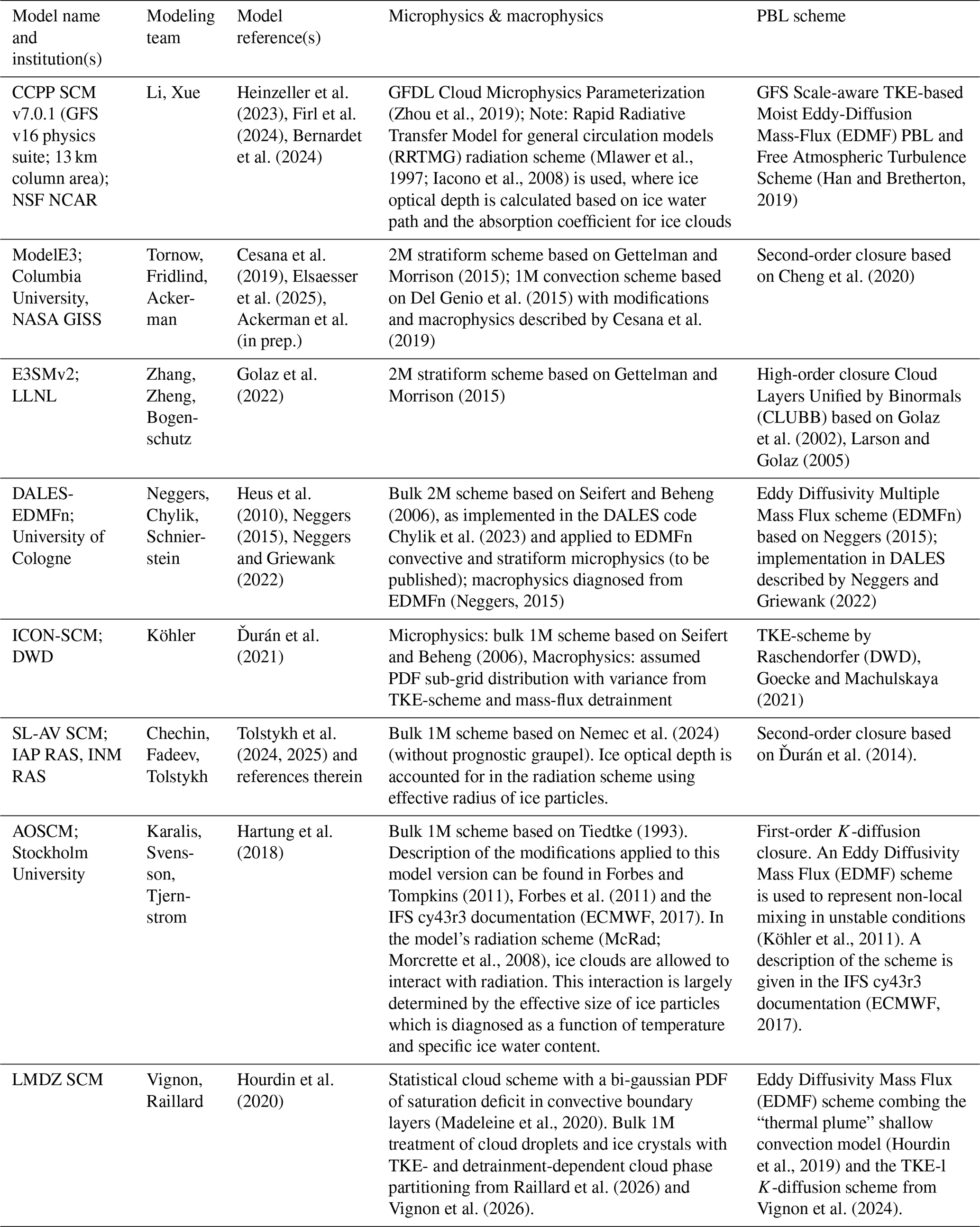
Tables 2 and 3 summarize the LES and SCM models, respectively, participating in COMBLE-MIP. In each table we also include details regarding the microphysical (and macrophysical for SCMs) parameterizations and turbulence closure approaches for each model.

Morrison et al. (2005, 2009b)Khairoutdinov and Kogan (2000)Verlinde and Cotton (1993)(Deardorff, 1980)Stevens (2002)Morrison et al. (2009b)Morrison and Grabowski (2008)Seifert and Beheng (2001)Seifert (2008)(Kirkpatrick et al., 2006)Khairoutdinov and Randall (2003)Morrison et al. (2005)Ovchinnikov et al. (2014)(Smagorinsky, 1963)Heus et al. (2010)Seifert and Beheng (2006)(Chylik et al., 2023)(Fu and Liou, 1993)(Schnierstein et al., 2024)(Deardorff, 1980)Dipankar et al. (2015)Seifert and Beheng (2006)(Fu, 1996)(Smagorinsky, 1963)Mortikov et al. (2019)Kadantsev et al. (2021)Voevodin et al. (2023)Lin et al. (1983)Grabowski and Smolarkiewicz (1999)Seifert and Beheng (2001)(Fu, 1996)Tkachenko et al. (2021)Savre et al. (2014)Seifert and Beheng (2006)Lilly (1992)(Stevens et al., 2002)Bryan and Fritsch (2002); Morrison and Milbrandt (2015)Morrison and Milbrandt (2015)Deardorff (1980)Seiki and Nakajima (2014)(Smagorinsky, 1963)Stevens et al. (1999, 2005)Stevens and Seifert (2008)Seifert and Beheng (2001, 2006)Seifert (2008); Seifert et al. (2012, 2014)(Tonttila et al., 2017; Ahola et al., 2020)(Smagorinsky, 1963)

Table 2 LES models participating in COMBLE-MIP. Abbreviations: one-, two-moment (1M, 2M) and turbulence kinetic energy (TKE).

Heinzeller et al. (2023)Firl et al. (2024)Bernardet et al. (2024)(Zhou et al., 2019)(Mlawer et al., 1997; Iacono et al., 2008)(Han and Bretherton, 2019)Cesana et al. (2019)Elsaesser et al. (2025)Gettelman and Morrison (2015)Del Genio et al. (2015)Cesana et al. (2019)Cheng et al. (2020)Golaz et al. (2022)Gettelman and Morrison (2015)Golaz et al. (2002)Larson and Golaz (2005)Heus et al. (2010)Neggers (2015)Neggers and Griewank (2022)Seifert and Beheng (2006)Chylik et al. (2023)(Neggers, 2015)Neggers (2015)Neggers and Griewank (2022)Ďurán et al. (2021)Seifert and Beheng (2006)Goecke and Machulskaya (2021)Tolstykh et al. (2024, 2025)Nemec et al. (2024)Ďurán et al. (2014)Hartung et al. (2018)Tiedtke (1993)Forbes and Tompkins (2011)Forbes et al. (2011)(ECMWF, 2017)(McRad; Morcrette et al., 2008)(Köhler et al., 2011)(ECMWF, 2017)Hourdin et al. (2020)(Madeleine et al., 2020)Raillard et al. (2026)Vignon et al. (2026)(Hourdin et al., 2019)Vignon et al. (2024)

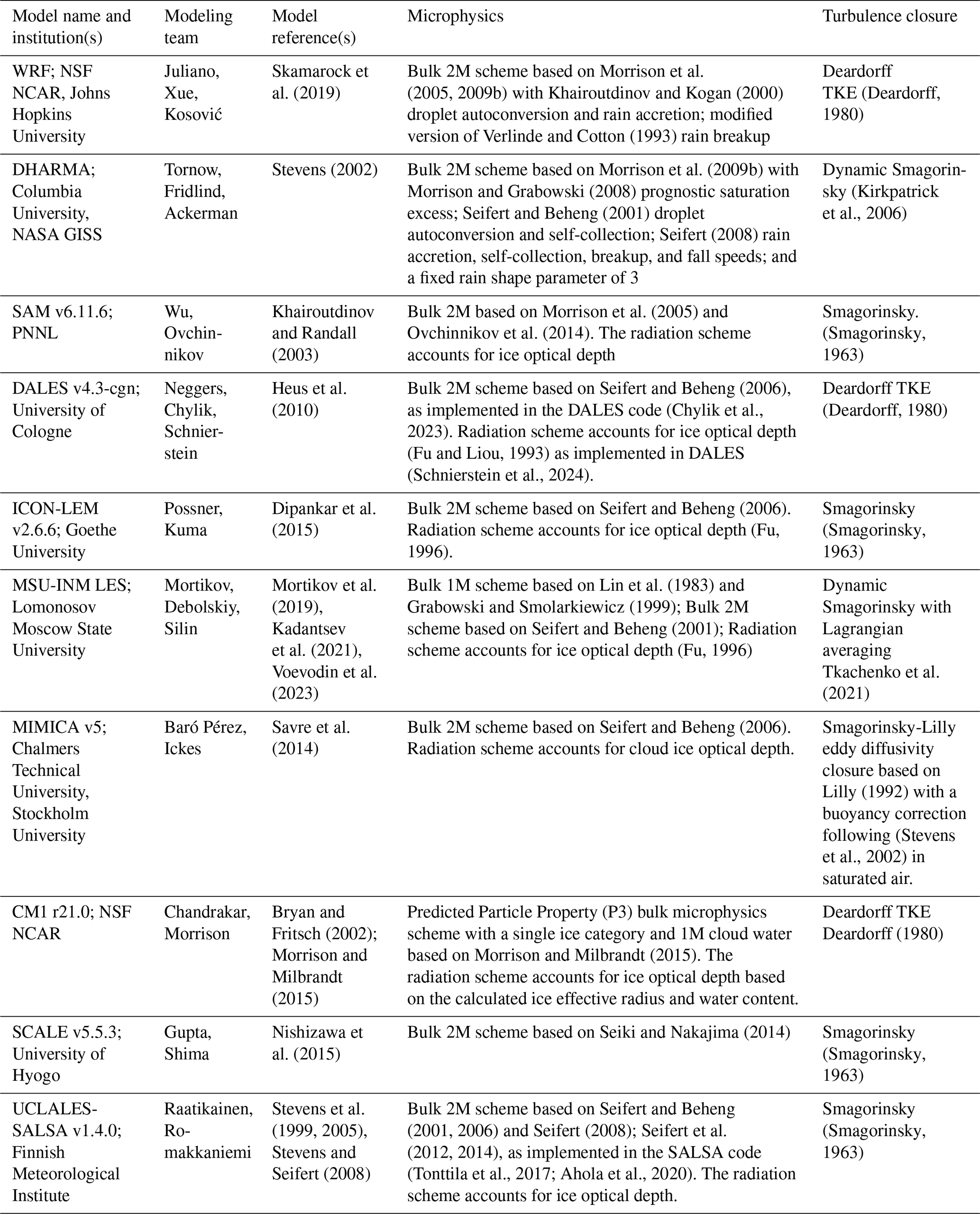
Table 3 SCM models participating in COMBLE-MIP. Abbreviations: planetary boundary layer (PBL).

2.4 Observational constraints

2.4.1 COMBLE measurements

COMBLE measurements at the AMF-1 site were near-continuous and comprised a suite of active and passive remote sensing instruments. In addition, radiosondes were launched every 6 h and provided vertical profiles of temperature and water vapor.

More specifically, we rely on two LWP retrievals from KAZR measurements in combination with ground-based microwave radiometry (MWR) from two retrievals (Johnson and Jensen, 2019; Zhang, 2019) as well as KAZR-retrieved cloud-top height (Johnson and Jensen, 2019), which we also translate into cloud-top temperature using coinciding radiosonde profiles (Keeler et al., 2022). From the multi-instrument ARM Radiative Flux Analysis (Riihimaki et al., 2019) product, we extract cloud optical depth retrievals. Sky radiometers obtain downwelling radiative fluxes at the surface (Sengupta et al., 2016). The Eddy Correlation Flux Measurement System (Sullivan et al., 2019) and the ARM Best Estimate Data (Chen and Xie, 1993) product provide turbulent surface fluxes. The latter data set also includes hourly surface precipitation rates. Atmospheric Emitted Radiance Interferometer (Shippert and Zhang, 2019) measured spectrally resolved downwelling infrared radiances, providing retrievals of vertical temperature and water vapor profiles.

COMBLE observations provide a single data point at 18 h, when the quasi-Lagrangian trajectory intersected the AMF-1 site. Above products were typically gathered over a window of 12 h centered around the arrival time, except for AERI with a 1 h window; allowing us to provide mean values and an uncertainty computed from the interquartile range (shown as error bars).

In addition to retrievals, we utilize c-level measurements from KAZR and the Micropule Lidar (MPL) to compare against forward-simulations of these observables using the Earth Model Column Collaboratory (EMC²; Silber et al., 2022) applied to LES and SCM output.

2.4.2 Reanalysis Products

To assess simulated surface fluxes, we colocate turbulent sensible and latent heat fluxes from the Copernicus Arctic Regional ReAnalysis (CARRA, Schyberg et al., 2020) dataset driven by the regional HARMONIE-AROME weather forecasting model (Gleeson et al., 2024) and ERA5 (Hersbach et al., 2020) driven by the global European Centre for Medium-Range Weather Forecasts (ECMWF) Integrated Forecasting System (IFS).

2.4.3 Satellite retrievals

To provide observational constraints upwind of the AMF1 site, we rely on retrievals from overpassing low Earth orbit satellites. Large solar zenith angles (typically greater than 70°) prevented the use cloud retrievals based on visible imagery, such as MODIS (Moderate Resolution Imaging Spectroradiometer, MODIS Atmosphere Science Team, 2017a, b) and VIIRS (Visible Infrared Imaging Radiometer Suite, Viirs Atmosphere Science Team, 2021a, b). However, we select cloud cover (defined as the fraction of pixels with optical depth greater 2 over a (100 km)² domain) for solar zenith angles smaller than 75° as a target metric, under the assumption that pixel-scale retrieval accuracy is of secondary importance. We also explored the use of infrared-based brightness-temperature MODIS and VIIRS retrievals to infer cloud-top temperature (Appendix D), but found it to be of limited value, likely owing to surface contamination under consistently broken cloud decks that seemingly increases for greater pixel size. Instead, we rely on MAC-LWP instantaneous LWP retrievals from a fleet of satellites carrying low-frequency passive microwave satellite instruments (Elsaesser et al., 2017), collocated over a domain of (100 km)² of the coinciding position along the trajectory. Unlike many LWP products, the LWP provided in MAC is a total liquid condensate estimate (i.e., rain plus cloud water path). No attempt at ad hoc separation into “cloud” vs. “rain” results in a substantial decrease in uncertainty (but this does require that models output the full liquid column estimate for fair comparison). An additional novel implementation is a cross-talk bias correction, resulting in smaller errors arising from water vapor and surface wind radiometric signals. Passive microwave LWP is retrieved day and night, free of illumination issues, and – due to their low frequency – largely blind to frozen hydrometeors (O’Dell et al., 2008). A full discussion of the above features and uncertainties (on the order of 20 % for the total LWP) can be found in Elsaesser et al. (2017) and Greenwald et al. (2018). In addition, we collocated CALIPSO (Cloud-Aerosol Lidar and Infrared Pathfinder Satellite Type Orbiter) Lidar Level 2 active cloud retrievals (NASA/LARC/SD/ASDC, 2018), namely cloud-top height and its associated cloud-top temperature (i.e., via external reanalysis fields), cloud optical depth, and ice water path, based on the CALIOP (Cloud-Aerosol Lidar with Orthogonal Polarization) measurements. The latter two are limited to optically thin clouds, with recent algorithmic updates enabling retrievals under somewhat opaque conditions (i.e., τ<10, Young et al., 2018b). IWP retrievals rely on a temperature-dependent particle size relationship (Heymsfield et al., 2014) and exhibit generally greater uncertainty compared to cloud optical depth, though both products exhibit an interquartile range of retrieved values that approximately matches the their mean uncertainty. CALIOP’s narrow swatch intersected the trajectory relatively early at 1.5 h (i.e., far north at 78.7° N) and 3 h prior to the Lagrangian airmass translated at this location, where it likely sampled such thin clouds.

For wind speed 10 m above ocean surface, we use retrievals from Synthetic aperture radar (SAR) measurements onboard the Sentinel-1B satellite (Monaldo et al., 2016).

Aside from retrievals, we perform forward-simulations of CALIOP signals applied to simulations output that can be compared with Level-1 data, similar to ground-based active remote sensing. Lastly, we use day-night-band imagery from VIIRS (VIIRS Calibration Support Team (VCST), 2025a, b) to qualitatively assess cloud structure, in particular of early cloud rolls.

3 Results

3.1 Quasi-Lagrangian evolution

We begin by evaluating the evolution of the CAO air parcel as it begins its trajectory over ice before being exposed to ∼18 h of open ocean. Figures 2 and 3 show several domain-averaged time series of thermodynamic and cloud fields as represented by the LES and SCM models, respectively, for both liquid-only and mixed-phase simulations. In addition to turbulent surface fluxes and cloud properties, Fig. 3 also shows the area fraction of convective clouds in panel (q, r). Overlain on each panel are available reanalysis and measurements that are intended to evaluate mixed-phase simulations. Recall that time = −1 h and time = 0 h approximately represent the MIZ transition period, where the air mass moves from consolidated pack ice over to open ocean.

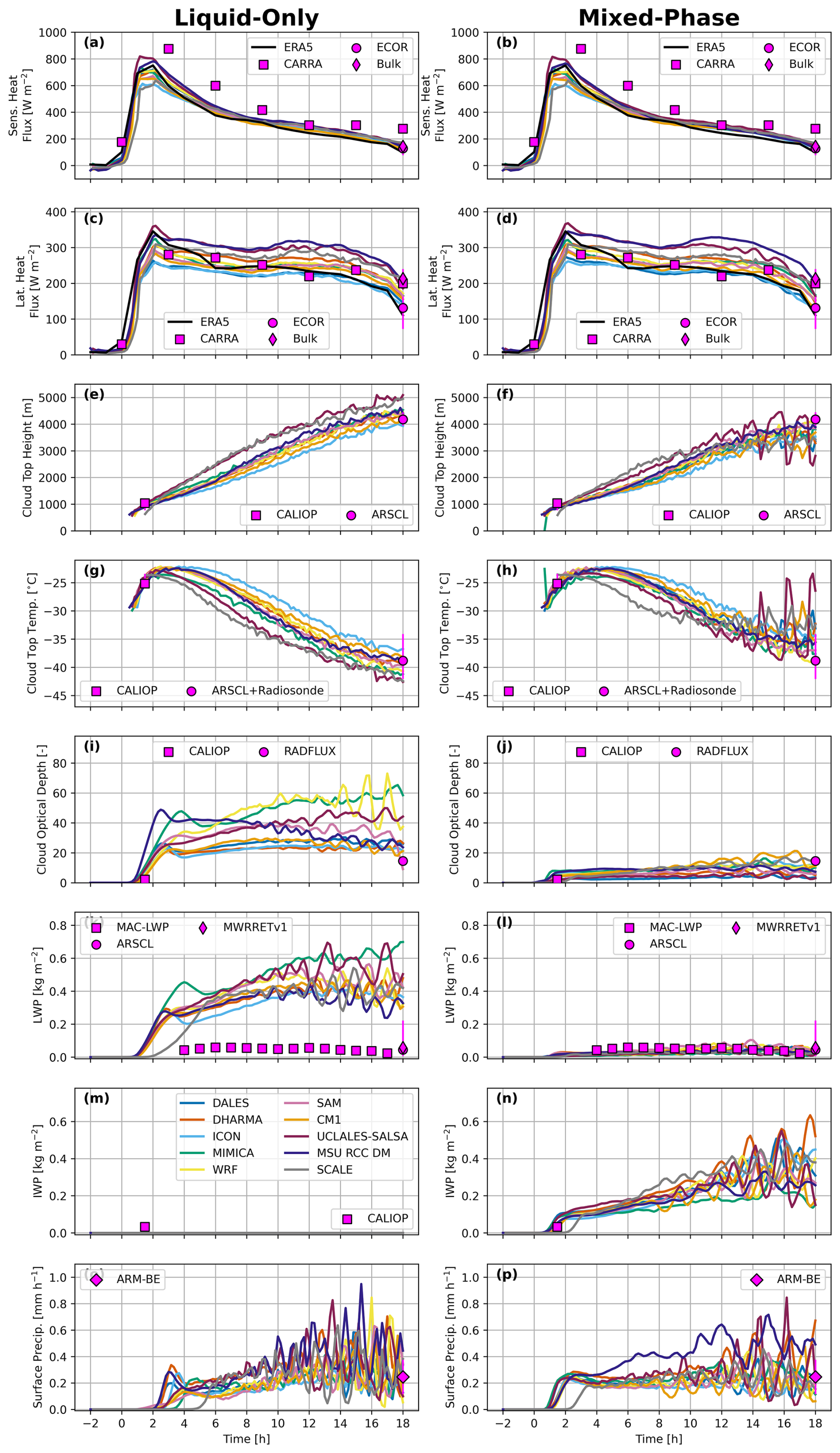
Figure 2 For LES liquid-only (left) and mixed-phase (right) simulations, time series of (from top to bottom): sensible heat flux, latent heat flux, cloud top height, cloud top temperature, cloud optical depth, LWP, IWP, and surface precipitation. LES models are plotted according to the legend in panel (m), while observations are also plotted according to the respective legends in each panel.

Figure 3 As in Fig. 2, except for the SCMs and the addition of of convective fraction.

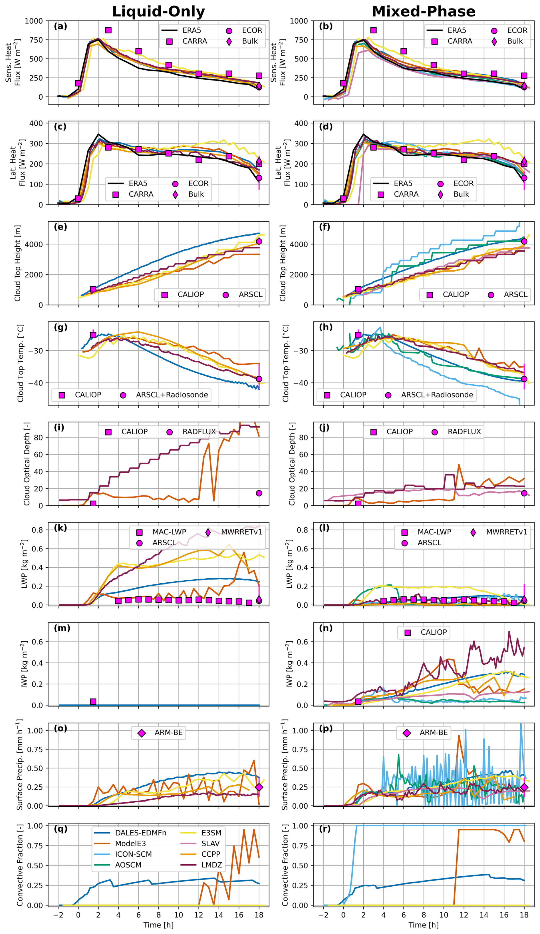
When the airmass (model domain) is over the ice, surface heat fluxes are weakly positive due to the relatively cold TSK. During this time, clouds have not yet developed in the model. Once the time-varying TSK begins to increase as the airmass moves over the MIZ, surface heat fluxes rapidly increase. Shortly after this time, clouds develop due to the intense turbulent mixing that ensues in response to the strong surface forcing. Sensible and latent heat fluxes quickly reach peak values of ∼650–800 W m⁻² and ∼275–350 W m⁻², respectively, by ∼1–2 h after the ice edge. During this time, the LES models and SCMs closely follow ERA5, which is not surprising since TSK is derived from ERA5. Meanwhile, CARRA shows larger sensible heat flux values 3 h after the ice edge, but its latent heat flux values are very much in line with the LES results. The BL is still relatively shallow (∼1000 m) during this time, owing to the limited cumulative surface heating. The LES models agree well with the CALIOP retrievals of cloud top height and temperature, as well as IWP, around 1.5 h after the ice edge; however, the models generally exceed observed cloud optical depth (note that CALIOP estimates are limited to τ<10).

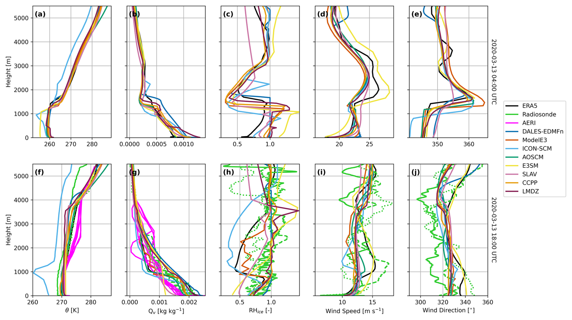
Vertical profiles 4 h after the ice edge (Fig. 4a–e for the LES models and Fig. 5a–e for the SCMs) show that the BL is convective (superadiabatic in the surface layer and thus well-mixed above), with a strong capping inversion. Not surprisingly, the LES models with stronger surface heat fluxes (UCLALES-SALSA and MSU) simulate warmer and moister BLs, resulting in similar relative humidity. Compared to ERA5, the LES models are generally cooler, moister, and shallower as a result of the initial condition (cf. Fig. 1b). The SCMs are tightly clustered with the exception of E3SM and ICON. The wind speed profiles, which agree well with ERA5, reveal strong shear near the surface, relatively uniform speeds in the middle of the BL, and again strong shear above the BL, where a jet is present. This jet, which initially formed over the ice (cf. Fig. 1c), remains intact even with the reduced baroclinicity downstream. The wind direction is from the north-northwest, turning clockwise with height below the jet due to frictional veering and counter-clockwise in the jet region due to cold-air advection.

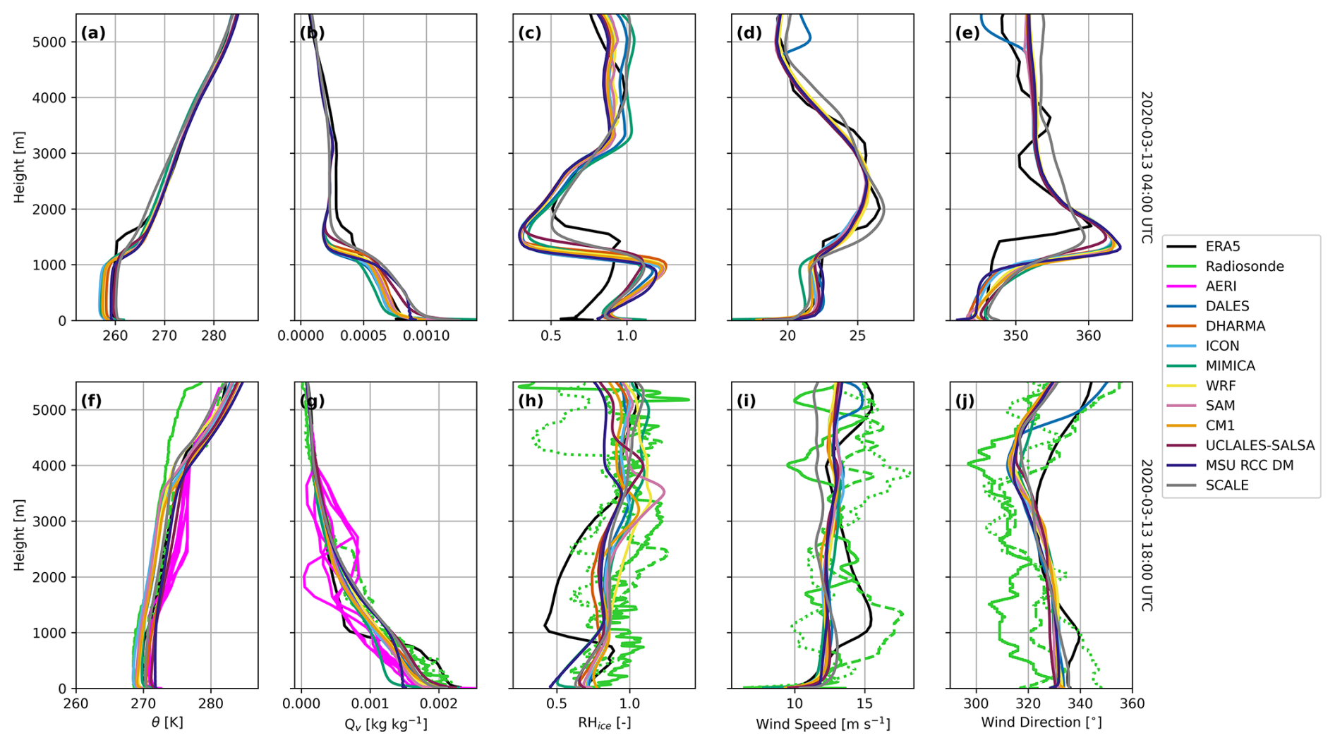
Figure 4 For the LES models, horizontally averaged vertical profiles of (from left to right): potential temperature, water vapor mixing ratio, relative humidity with respect to ice, wind speed, and wind direction. The top and bottom rows show results for 04:00 and 18:00 UTC, respectively. Observed profiles within a window of time (for radiosondes at 11:26, 17:36, and 23:22 UTC as solid, long-dash, and short-dash linetypes, respectively, and all profiles ±0.5 h for AERI as solid type) are shown as individual lines.

Figure 5 As in Fig. 4, except for the SCMs.

As the air mass continues its trajectory across the open ocean (Fig. 1a), surface sensible heat fluxes steadily diminish (Fig. 2b), as the air-sea temperature contrast shrinks (not shown). Latent heat fluxes diminish much more slowly (Fig. 2d). As a result of the accumulating heat input from the ocean to the atmosphere, the BL continues to grow nearly linearly in the LES models (Fig. 2f), while cloud top temperatures become commensurately colder (Fig. 2h, to be discussed in Sect. 4). All of the SCMs well reproduce the cloud-top deepening (Fig. 3f), with ICON-SCM, AOSCM, and DALES-EDMFn clustering closely and generating relatively large cloud-tops, and SLAV, E3SM, ModelE3, CCPP, and LMDZ clustering closely and generating relatively small cloud-tops.

MAC-LWP retrievals provide an important constraint on LWP from ∼4 h after the ice edge and beyond. Toward the beginning of this period, all LES models underestimate LWP (Fig. 2l). The SCMs show mixed results (Fig. 3l): E3SM continuously overestimates LWP, ModelE3 and CCPP continuously underestimate LWP, and DALES-EDMFn and LMDZ well reproduce LWP. AOSCM's LWP values jump near the beginning of the period (similar to E3SM), before reducing to near zero around 6 h. The MAC-LWP product shows mostly steady LWP values until the end of the period, at which point they begin to decrease; Sect. 5 will discuss the challenges connected to this evolution. Given the absence of IWP retrievals downwind of cloud formation, MAC-LWP forms a key constraint for cloud condensate. Most of the LES models represent this trend; however, LWP (and cloud top temperature and IWP) oscillations appear because the LES domains cannot resolve the relatively large convective cells that scale with domain size. The SCMs largely simulate this trend toward lower LWP values.

At the end of the trajectory (18 h after the ice edge), the model domains have arrived at the COMBLE deployment location in Andenes, allowing us to compare with the ground-based measurements. Mixed-phase LES models and SCMs are in very good agreement with both the ECOR and ARM Best Estimate Bulk surface heat and moisture flux measurements. KAZR retrievals of cloud top height (∼4000 m) and temperature ($\sim -\mathrm{38}$ °C with large variability), as well as liquid water path, suggest that the LES models and SCMs are within reasonable range. The LES slightly underestimate cloud top height and therefore overestimate cloud top temperature, while the SCMs cluster around the measurements, with the exception of ICON-SCM that overestimates deepening and underestimates cloud-top temperature. LWP values are also comparable between LES/SCM and ARSCL and MWRRETv1 estimations that are showing large variability due to the horizontally heterogeneous LWP field that corresponds with narrow, turbulent updrafts; large-domain simulations are expected to resolve such variability effects (as discussed in Sect. 5). Precipitation rates also demonstrate this heterogeneity; LES/SCM generally reproduce ARM Best Estimate retrievals. Lastly, a cloud optical depth of ∼15 from RADFLUX suggests that the LES models, which show large spread, underestimate this field. Out of the three SCMs that report optical depth, SLAV presents fairly steady values, agreeing well with RADFLUX-retrieved values. ModelE3 shows initially lower values compared to SLAV and then exceeds SLAV once the convective scheme takes over, thereby overestimating optical depth towards the end. LMDZ also shows initially lower values but increases sooner than ModelE, presenting the largest values bewtween 4–12 h.

The vertical atmospheric structure at the COMBLE field site (Fig. 4f–j) is drastically different than that at 4 h downwind of the ice edge. There the BL reaches up to ∼4000 m, where the section between 1000 and 4000 m appears neutral with respect to moist adiabatic processes. The strong inversion remains above the cloud layer. While it is no surprise that there is larger spread between the mixed-phase LES models and the SCMs 18 h downstream of the ice edge, agreement in the θ and q_v profiles is reasonable considering we did not impose any thermodynamic nudging. For the θ profile, ERA5 and two of the three radiosonde profiles are within the range of the LES models, while the third radiosonde profile bounds the lower limit of the LES models and the AERI retrievals bound the upper limits of the LES models. The radiosonde profiles show a slightly moister environment relative to the LES models below ∼3000 m, while AERI retrievals suggest a mostly drier environment. Still, the LES models are within a reasonable range considering observational uncertainty. A similar result is found with the SCMs, except DALES-EDMFn, CCPP, and LMDZ show a moister environment compared to other SCMs. The wind speed profile is less sheared (more vertically uniform) compared to radiosondes, with north-northwest winds that back with height, suggesting continued cold-air advection. Even though the wind speed and direction profiles deviate more substantially from ERA5 at the AMF1 site relative to the previous comparison time, radiosonde observations suggest that there is large variability. This is likely related to the location of sampling relative to the convective cells, which are spatially heterogeneous in their dynamic structure.

3.2 Comparison to liquid-only simulations

Compared to LES liquid-only simulations, mixed-phase ones show reduced cloud-top heights most prominently seen at the final stage (cf. Fig. 2e–f, by $\sim -\mathrm{1000}$ m at 18 h) and greater cloud-top temperatures (cf. Fig. 2g–h, by $\sim +\mathrm{5}$ K at 18 h); this response is largely absent in respective SCM output (Fig. 3e–h). This sensitivity is in line with previous research that suggests a precipitation-made MBL stratification that hinders vertical transport and corresponding deepening (e.g., Tornow et al., 2021). While surface precipitation rates are largely unchanged between liquid-only and mixed-phase simulations, we note that cloud-base precipitation rates are greater in mixed-phase simulations (not shown), implying a greater sub-cloud sublimation compared to sub-cloud evaporation in liquid-only simulations (Fig. 6a), which results in a greater vertical moisture stratification in mixed-phase simulations, measured as the difference in water vapor mixing ratio at 25 % and 75 % of the cloud-top height (Fig. 6b).

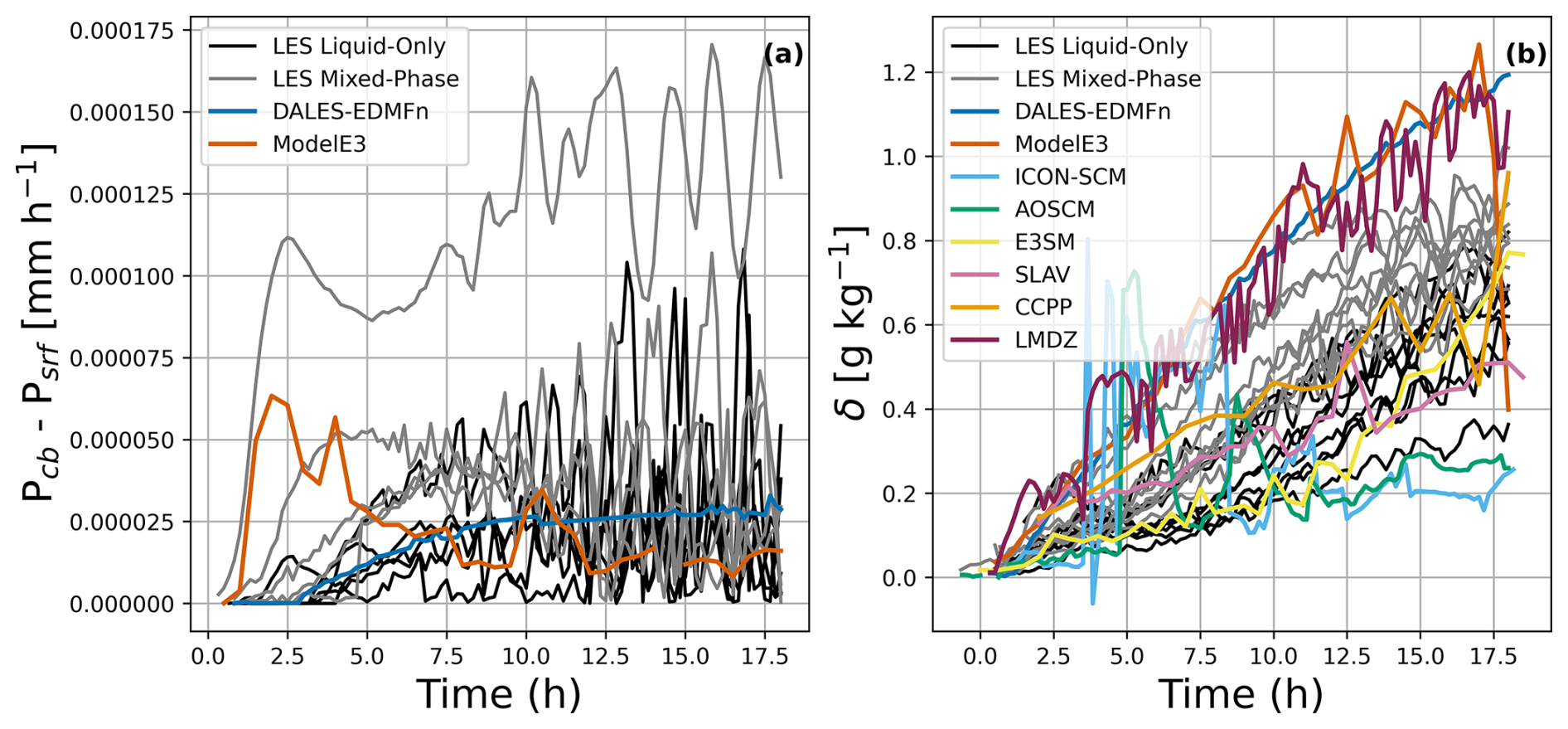
Figure 6 Cloud-base minus surface precipitation rate (left) and water vapor mixing ratio difference between the bottom and top of the MBL (i.e., 25 % and 75 % of cloud-top height, respectively) (right) over time. LES Liquid Only and LES Mixed-Phase simulations are shown in the black and gray lines respectively, with each line representing results from a single model, while the mixed-phase SCMs are colored according to the legend, noting that not all models reported precipitation flux profiles.

Liquid-only simulations naturally produce greater LWP values compared to mixed-phase simulations. While SCMs (Fig. 3k–l) qualitatively capture this response, there are stark differences across models. For example, ModelE increases its LWP from 0.025 to 0.1 g m⁻² while removing an IWP of 0.025–0.4 g m⁻². In contrast, E3SM increases its LWP from 0.2 to 0.4 g m⁻² while removing an IWP of 0.025–0.25 g m⁻². Section 3.5 will quantify the resulting radiative response.

Differences in cloud condensate amount and phase also modify temperature profiles via cloud radiative effects and microphysical latent heat release (e.g., shown illustratively in Fig. D1). Specifically, mixed-phase simulations exhibit reduced cloud-top longwave cooling and enhanced warming below cloud-top. Simultaneously, microphysical latent heat release warms the cloud layer while cooling the region below cloud base, resulting in stronger temperature stratification. Ultimately, these combined changes in radiative forcing and latent heating can further suppress cloud-top entrainment and vertical mixing in mixed-phase simulations.

3.3 Mesoscale organization

During the ∼1000 km open ocean fetch of the 13 March case, the cloud structures underwent a clear transition from rolls to cells. In this section, we will discuss the organization of these convective structures as represented by the LES models. SAR, whose retrievals are used to estimate wind speeds at 10 m above the ocean surface, as well as visible satellite imagery, are used to evaluate the extent to which LES is capable of representing the structures.

3.3.1 Rolls

Clouds streets associated with BL rolls emanating from the MIZ are a prominent feature of most CAOs observed during COMBLE via satellite imagery, including on 13 March. However, simulating rolls has proven to be elusive for LES models. This problem was encountered, for example, during the CONSTRAIN model intercomparison by de Roode et al. (2019), who concluded that “the reason that no cloud streets are present in the simulations is not fully understood by the authors”.

Satellite imagery from 13 March indicates that BL rolls were likely present in the clear air prior to cloud formation, and they were variable in space and time (Fig. 1a in  Lackner et al., 2023a). Alignment was primarily NNW-SSE with a less common secondary mode aligned NE-SW. According to the classification suggested by Young et al. (2002), these rolls exhibited a “band of froth” appearance associated with an aspect ratio of roll wavelength on BL depth (z_i)>1 and multiple updrafts spanning each cloud street. At 2 h from the ice edge, the BL height was ∼1 km (per CALIPSO), and the roll wavelength was approximately 5 km (not shown), leading to an aspect ratio of 5, in agreement with marine CAOs reported by Young et al. (2002) (see their Fig. 4). In the following 2 h, the aspect ratio similarly increased faster than the simulated BL depth (cf. their Fig. 4 with BL depth increasing). Results from our LES on a modest domain (25×25 km²) might be expected to contain ∼4 cloud streets at 4 h downwind of the ice edge (BL height of ∼1.3 km). We see slight evidence of rolls at this time in DHARMA (Fig. 7, top row), but they are much narrower than in the VIIRS satellite observations. UCLALES-SALSA shows less organization. Pseudo-albedo values are comparable between VIIRS and LES, with a rather homogeneous cloud field. Meanwhile, SAR imagery around this time (Fig. 7, top row) shows streaky wind speed structures that are somewhat unorganized but nonetheless much larger than what is modeled by the LES.

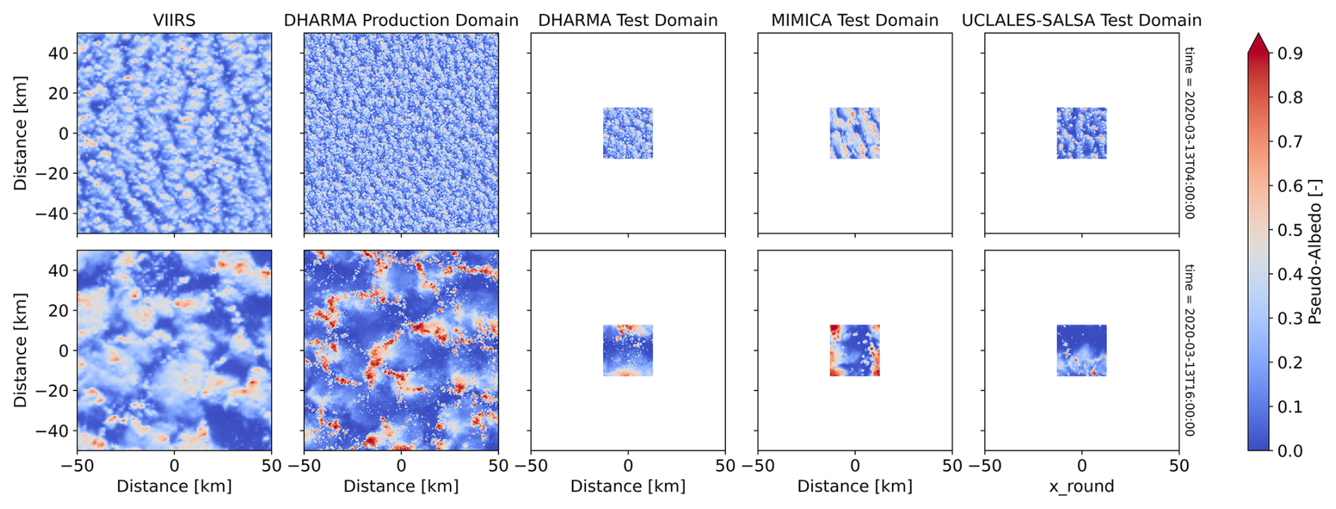
Figure 7 Pseudo-albedo comparison between VIIRS and DHARMA, MIMICA, and UCLALES-SALSA LES models at (top) 04:00 (rolls) and (bottom) 16:00 UTC (cells).

Negligible improvement in simulating the roll structures was found for sensitivity tests with horizontal winds nudged to ERA5 profiles or other setup changes as follows (not shown). Sensitivity tests included (1) a sharper and lower inversion over sea ice (positing that ERA5 may contain high biases of inversion height, z_i, over sea ice); (2) changes to sea surface temperature evolution downwind of the ice edge (a weaker gradient); (3) increase in horizontal resolution (to 25 m grid cell spacing); (4) increase in domain size to 100×100 km² (Fig. 7b); (5) adding an idealized Ekman spiral in the initial condition (obtained from a 1D model, again positing biases in ERA5); and (6) changes to the surface roughness specification. Furthermore, realistic simulations using WRF with a nested internal domain exhibit stronger cloud streets than our MIP LES setup with periodic boundary conditions, but they remain weaker than observed (not shown). We note that recent quasi-Lagrangian LES conducted with DHARMA for a CAO case study off over the Northwest Atlantic readily reproduced MBL rolls without any special attention to setup details (not shown). However, the rolls in that case were not present when clouds first formed off-shore, suggesting a different formation process.

Under conditions of large stability parameter ($-z_{\mathrm{i}}/L\sim \mathrm{10}$), where L is the Monin-Obukhov length, Gryschka et al. (2008) used LES to show that roll formation requires triggering by sea ice temperature heterogeneities. They referred to such rolls as forced, in contrast to self-organizing rolls that occur when surface fluxes are weaker. At 4 h downwind of the ice edge, the 13 March case exhibited z_i of approximately 1300 m and L of approximately −100 m, consistent with stability parameter ∼10, placing this case into the forced category. In follow-on work, Gryschka et al. (2014) compare simulations with and without roll-generating sea ice heterogeneity, and conclude that total surface fluxes do not significantly differ because the rolls assume part of the transport that is otherwise turbulent rather than organized. They therefore suggest that forced roll convection is not necessary to include in weather and climate model parameterization schemes. In our 13 March 2020 COMBLE case, sensitivity experiments with the SAM model by the PNNL group demonstrated that imposing periodic cross-wind fluctuations in surface fluxes mimicking the MIZ can force the formation of the cloud rolls but the cloud structure is short-lived and disappears quickly when the air column moves over the open water with uniform SST (not shown).

Gryschka et al. (2008) mention that along-roll wind shear or shear curvature below 0.2z_i may also lead to forced rolls in the absence of upwind surface heterogeneity. Young et al. (2002) further conclude that candidate processes contributing to the range of observed atmospheric roll behaviors include surface buoyancy flux, latent heat release, roughness-induced shear, and baroclinically induced shear, as well as tropospheric gravity waves that may undergo three different trapping mechanisms and whose effects may depend on the angle between the shear vector within the BL versus above. While DHARMA simulations do exhibit strong gravity waves under both Northwest Atlantic CAO conditions (not shown) and in the 13 March case (Fig. 7), observations of ice edge and thermodynamic and wind profile conditions are lacking to confirm apparent shortfalls in the case specification. Finally, mechanisms associated with ice edge heterogeneity could be difficult or impossible to represent in quasi-Lagrangian LES with fully periodic boundary conditions.

3.3.2 Cells

Farther downwind, the convective rolls transitioned into cells due to a number of potential factors discussed in Sect. 1. To more carefully examine the well-developed cellular structures from the 13 March case, we again rely on VIIRS imagery (Fig. 7, bottom row) and SAR retrievals (Fig. 8, bottom row) and focus on 16 h downstream of the ice edge. By this time, the structures were relatively large with observed cell sizes of ∼20–40 km, in accordance with previous studies by Wu and Ovchinnikov (2022) and Juliano et al. (2024). The modest LES domains are much too small to properly represent the large cellular structures, which now scale with the domain size. For reference, we again show DHARMA's production-sized domain, which is able to fully capture cell-cell interactions. These findings are aligned with de Roode et al. (2004), who found that a model domain must be several times larger than the scales of interest if one wants to properly simulate their physics.

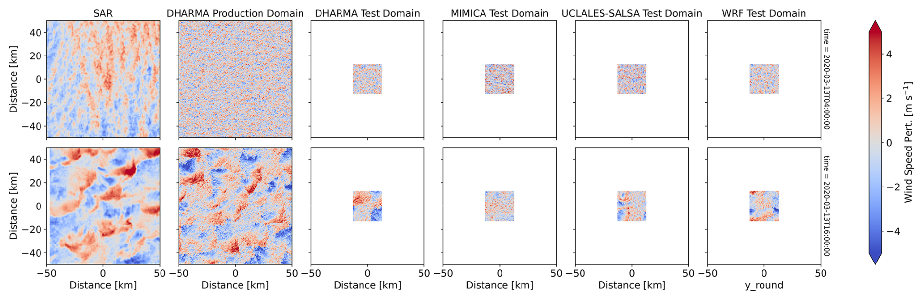
Figure 8 10 m wind speed perturbation comparison between SAR and DHARMA, MIMICA, UCLALES-SALSA, and WRF LES models at (top) 04:00 (rolls) and (bottom) 16:00 UTC (cells). The 10 m wind speed perturbation field is computed by subtracting the domain-averaged value from each grid cell.

Peak pseudo-albedo values (Fig. 7) from the models are larger than those values estimated from the VIIRS retrievals. The reason for this could be (1) the simplified approximation of albedo that we applied to narrow-band VIIRS radiances, (2) assumptions in LES albedo that are potentially erroneous, such as assumed particle size, and (3) LES clouds that could be optically too thick. The SAR wind field highlights the low- and high-wind speed regions associated with the enlarged cell structures. By this point, the field was much more horizontally homogeneous than before, with wind speed perturbation magnitudes of approximately ±4 m s⁻¹. The LES models generally capture the magnitude of the wind speed perturbations; however, only the production domain is large enough to sufficiently resolve the cell structures. Moreover, the corresponding modeled LWP values in the production domain reveal the tight connection between the dynamics and macrophysics: regions of low-level convergence are tied to liquid water production. High-resolution mesoscale simulations of this case also revealed a similar relationship (Juliano et al., 2024). Unfortunately, the modest domains are too small to show this connection on the mesoscale.

3.4 Connecting surface forcing with cloud growth

To highlight the impact of surface-based forcing on the evolution of vertical cloud development in this intense CAO case, in Fig. 9 we plot cumulative sensible and latent heat fluxes versus cloud-top height. The LES results from the liquid-only simulations and mixed-phase simulations are shown in black and gray lines, respectively, while the SCM results are colored according to the respective model.

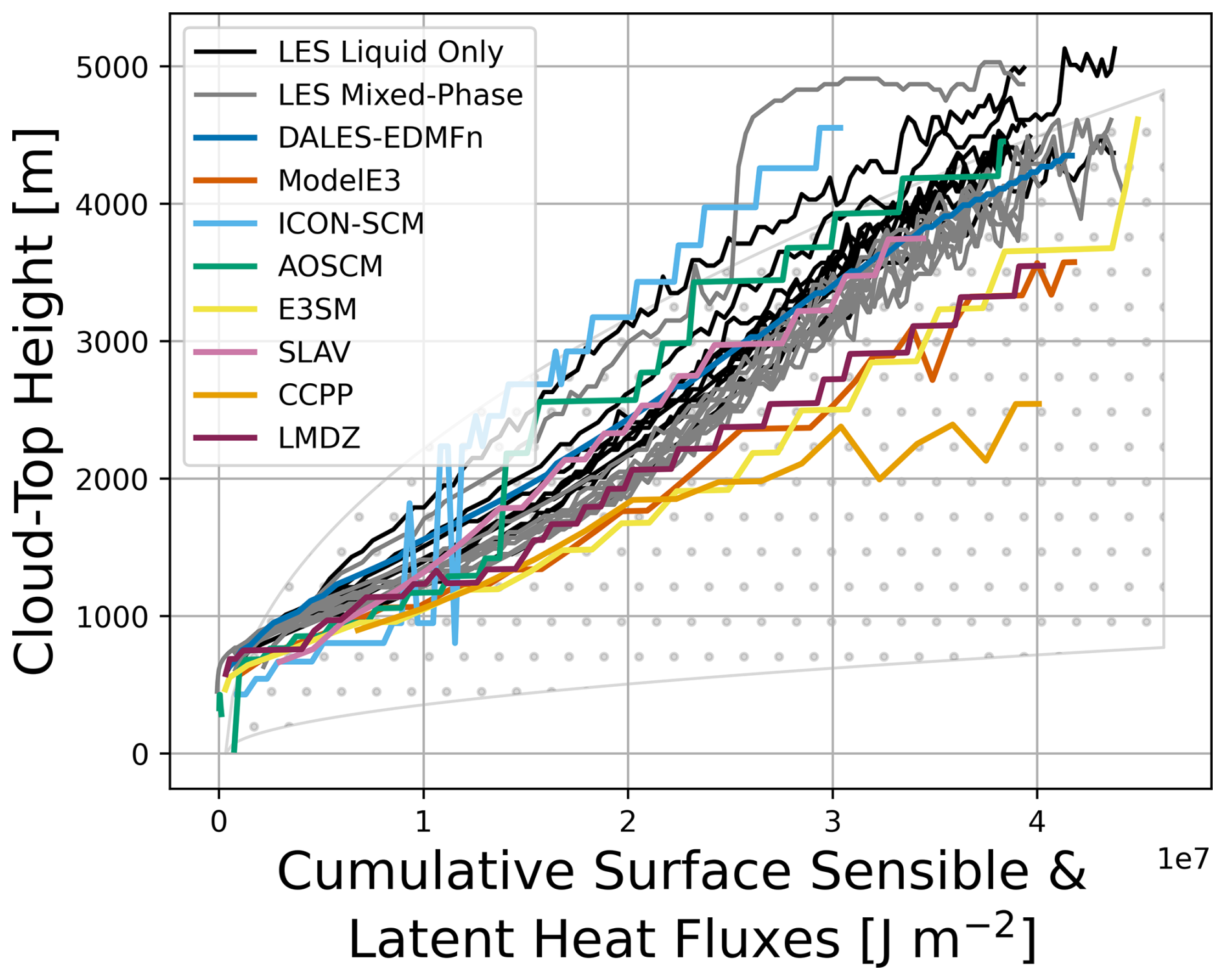
Figure 9 Relationship between cumulative surface heat (sensible and latent) fluxes and cloud-top height. LES Liquid Only and LES Mixed-Phase simulations are shown in the black and gray lines respectively, with each line representing results from a single model, while the SCMs are colored according to the legend. Stippling in the background shows theoretical expectations assuming surface-only forcing (Eq. 11.2.2f in Stull, 1988) under weakest and strongest conditions.

We find a near-linear relationship between surface heat and moisture input to the system and vertical cloud growth. This growth partially exceeds parabolic growth from theoretical expectation under surface-only forcing (cf. stippling in Fig. 9). In general, clouds in the liquid-only LES are slightly deeper than those in the mixed-phase LES, owing to initially more rapid growth in liquid-only runs; previous modeling connected the presence of frozen hydrometeors with greater MBL stratification, reduced vertical transport, and muted deepening (e.g. Tornow et al., 2021; Wu et al., 2025). The SCMs generally reproduce the LES relationship, albeit with more spread about the cloud-top height evolution. ICON-SCM produces the deepest clouds despite some of the lowest cumulative heat fluxes. AOSCM, DALES-EDMFn, and SLAV fall within the range of the LES models, while E3SM, ModelE3, CCPP, and LMDZ broadly produce lower cloud-top heights.

3.5 Cloud-radiative feedbacks

We now examine the temporal evolution of modeled and observed LW radiative fluxes. Figure 9 shows the top of atmosphere (TOA) upwelling LW fluxes and surface downwelling LW fluxes for both the liquid only and mixed-phase simulations. Also plotted are TOA upwelling LW fluxes measured by CERES.

We first discuss the TOA upwelling LW fluxes (Fig. 10a, b). At the beginning of both the liquid only and mixed-phase simulations, when the airmass is over the cold ice surface and clouds have not yet formed, TOA upwelling LW fluxes range between ∼165 and 185 W m⁻² (an outlier of ∼215 W m⁻² is modeled by E3SM). As the airmass moves over the relatively warm surface of the open ocean, the column remains cloud-free for a short period of time, at which point the LW fluxes rapidly increase. Once clouds develop around time = 2 h, the LW fluxes quickly decrease, as clouds, whose tops are ∼1000 m a.s.l., contribute smaller fluxes at TOA. In the liquid only simulations, the LW fluxes remain approximately constant or slowly decrease for a few hours before more strongly decreasing as the cloud-top heights increase. All of the models – both LES and SCM classes – show a similar trend. If we normalize each time series by its pre-cloud state (time = −1 h), then the similarities between models become even more apparent (Fig. 11a). Meanwhile, CERES measurements show approximately constant values around ∼170–180 W m⁻² from time = 5 to 8 h, values increasing to ∼190 W m⁻² by time = 11 h, and finally decreasing to ∼175 W m⁻² by time = 18 h. Thus, the liquid only simulations drastically underestimate TOA upwelling LW fluxes in the last ∼8 h of the simulation.

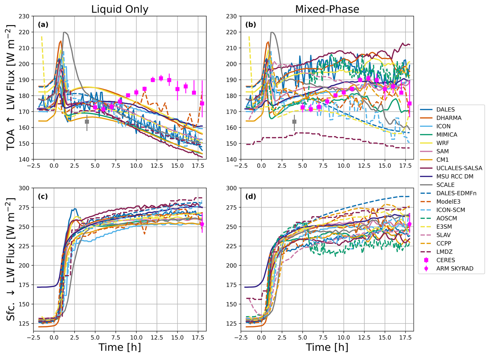
Figure 10 Time series of (top row) TOA upwelling LW fluxes and (bottom row) surface downwelling LW fluxes for (left column) Liquid Only simulations and (right column) Mixed-Phase simulations. LES models (solid lines) and SCMs (dashed lines) are colored according to the legend. ARM SKYRAD and CERES observations co-located with the model domains in space and within 1 h time are shown by the magenta markers. The gray marker represents a CERES retrieval potentially biased by a high solar zenith angle. The markers represent the mean value spanning the LES domain while the bars represent the interquartile range.

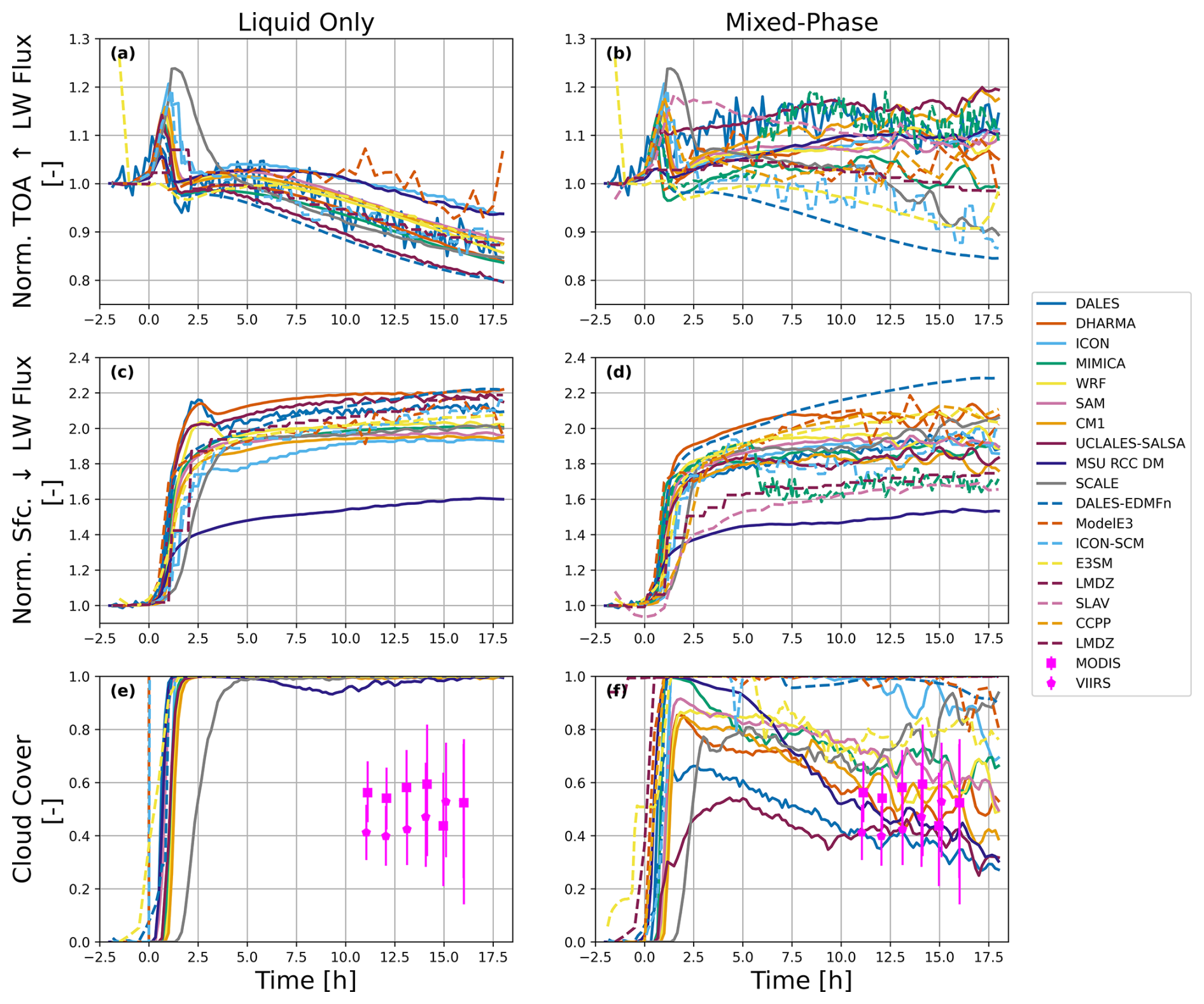
Figure 11 As in Fig. 10, except showing only model results that are normalized by the pre-cloud ($t=-\mathrm{1}$ h) values. In the bottom-most row, we also show the modeled cloud cover together with observational targets, inferred from satellites carrying the MODIS and VIIRS instruments. Identical to LES, cloud cover is computed as the portion of pixels with a cloud optical depth greater than 2.0.

In the mixed-phase simulations, a much more complicated picture emerges: as soon as SST increases, the simulated TOA LW upwelling fluxes may increase, and – as clouds form, fill in, and break apart – remain approximately constant, or decrease in time depending upon the model (Fig. 10b). Overall, the biases are smaller between the models and the CERES observations; however, the mixed-phase simulations show much wider inter-model spread. For example, LMDZ generally follows the majority of models but shows smaller TOA LW fluxes, likely linked to a thin layer composed of frozen hydrometeors further aloft (not shown). Normalizing each time series by its pre-cloud state (time = −1 h) further highlights the large spread (Fig. 11b) relative to the liquid-only simulations (Fig. 11a). In the following paragraphs, we describe potential reasons for these differences.

The time series of surface downwelling LW fluxes show minimum values during the pre-cloud state in both the liquid only (Fig. 10c) and mixed-phase (Fig. 10d) simulations. In the liquid only case, LW fluxes rapidly increase once clouds form, before plateauing around time = 5 h and increasing only minimally with time thereafter. Compared to ARM SKYRAD measurements about half of the models overestimate by about 10–20 W m⁻². The mixed-phase case shows a similar trend, with much greater spread between models and somewhat smaller values that straddle ARM SKYRAD measurements. The normalized plots for the downwelling LW fluxes (Fig. 11c, d) again highlight the relatively large spread induced by introducing ice microphysics into the simulations.

To clarify the direct impact of ice microphysics on the simulated LW fluxes, we show the ratio of the TOA upwelling (Fig. 12a) and surface downwelling (Fig. 12b) fluxes. The ratio is computed as the values from the liquid-only simulations divided by those from the mixed-phase simulations (ratios greater than 1 indicating larger LW fluxes for the liquid only case). In almost all simulations, regardless of model class, and for the entirety of the time series, TOA upwelling LW flux ratios are <1; in other words, adding ice microphysics results in monotonically increasing LW escaping at TOA, in line with earlier modeling work on quiescent Arctic clouds (Eirund et al., 2019). LMDZ initially shows a ratio greater than 1 due to the aforementioned thin layer of high-altitude clouds. Despite SCMs largely overlapping the LES for liquid only conditions, as a class they depart from LES in predicting less effect of ice on TOA upwelling LW fluxes. At the surface, the downwelling LW flux ratios begin to diverge once cloud develops and then remain mostly constant beyond time = 5 h.

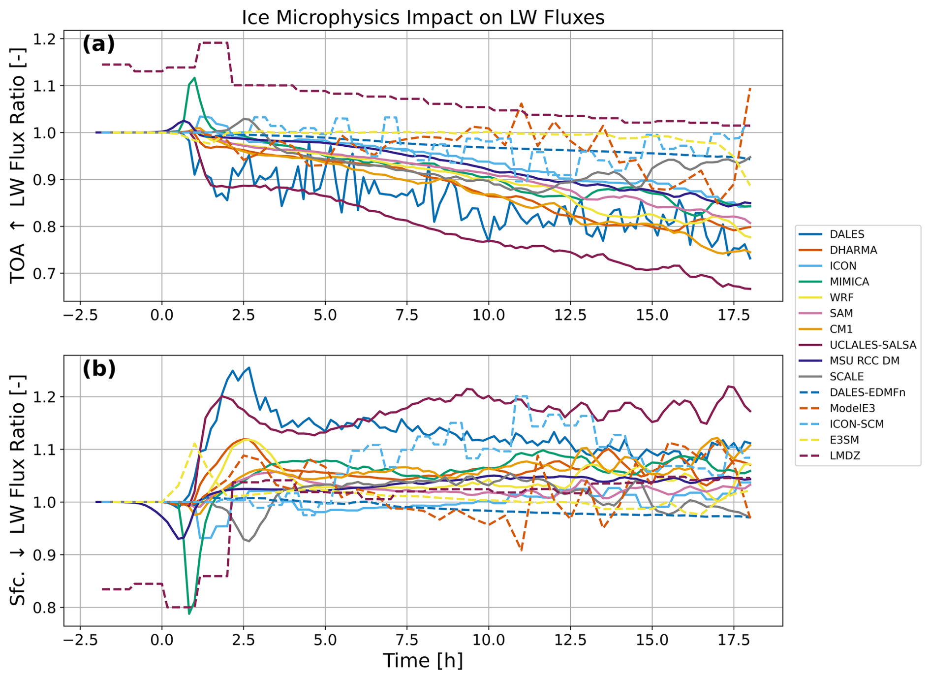
Figure 12 Time series of (top row) TOA upwelling LW flux ratio and (bottom row) surface downwelling LW flux ratio. The ratio is computed as the Liquid Only result divided by the Mixed-Phase result. That is, for a given model, a ratio value larger than 1 indicates that the value of the respective variable is larger in the Liquid Only simulation than in the Mixed-Phase simulation.

Cloud cover (for LES defined as the fraction of columns with τ>2), which is a key quantity controlling the TOA upwelling and surface downwelling LW fluxes, is plotted in Fig. 11e, f for the liquid-only and mixed-phase cloud simulations, respectively. In the liquid only case, for all LES and SCM models, cloud cover quickly increases to 1 (completely overcast) off the ice edge. Cloud cover remains overcast for nearly all models throughout the simulation. In contrast, the mixed-phase case produces varying responses depending upon the model. Broadly speaking, the SCMs give higher cloud cover than the LES models, with most LES not reaching a completely overcast cloud deck and diminishing to ∼0.3–0.6 cloud cover.

In Fig. 13, we more explicitly show the control of cloud cover on surface and TOA LW flux ratios by averaging the values over the final 2 h of the simulation for each model (Fig. 13a, d). In addition, we include the control of all-sky optical depth on the LW flux ratios in Fig. 13b, e. Lastly, we present how cloud-top height changes relate to LW flux ratios (Fig. 13c, f). Once again, we compute cloud cover ratios of liquid-only to mixed-phase simulations. These figures confirm that cloud cover, optical depth, and cloud-top height all have first order effects on the LW fluxes. Models with higher cloud cover ratio (i.e., ice microphysics leading to more cloud breakup) produce larger TOA upwelling LW fluxes because gaps in the cloud deck lead to a larger contribution from the relatively warmer, lower levels, particularly the ocean surface. From the surface perspective, more gaps in the cloud deck lead to more contribution from clear-sky, free-tropospheric downwelling LW fluxes (lower temperatures). Interestingly, even though the LES models display clear relationships in Fig. 13a, c, the bias across SCM models is consistent, suggestive that SCMs essentially do not know about mesoscale cloud structure (i.e., cloud macrophysical changes driven by the presence of frozen hydrometeors) or at least fail to represent its effect on cloud cover and by extension LW fluxes, with some smaller differences potentially stemming from varying cloud cover definitions (of “cf.”) across SCMs.

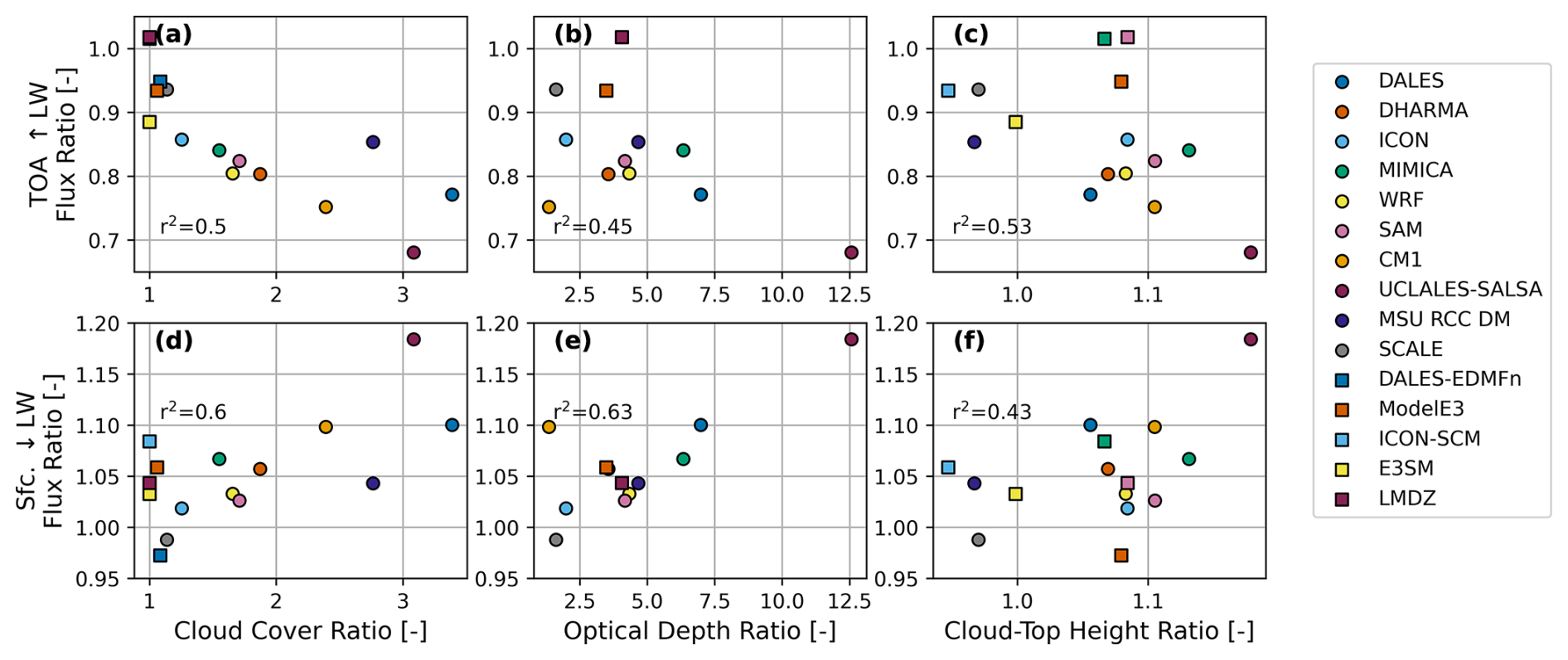
Figure 13 Relationships between (top left) cloud cover ratio and TOA upwelling LW flux ratio; (top middle) optical depth ratio and TOA upwelling LW flux ratio, and (top right) cloud-top height ratio and TOA upwelling LW flux ratio; (bottom right) optical depth ratio and surface downwelling LW flux ratio; (bottom middle) cloud cover ratio and surface downwelling LW flux ratio, and (bottom right) cloud-top height ratio and downwelling LW flux ratio. Like Fig. 12, ratios are computed as the Liquid Only result divided by the Mixed-Phase results. LES models and SCMs are shown in circles and squares, respectively. Fractions of explained variance, r², are shown for only the LES models.

With regard to the effect of changes in optical depth between the liquid-only and mixed-phase simulations on the LW fluxes, a similar story emerges (Fig. 13b, e). Including ice in the simulations greatly reduces optical depth, leading to more upwelling LW radiation reaching TOA due to a larger contribution from surface LW emissions. The reduction in optical depth also allows for greater contribution from above-cloud downwelling LW fluxes at the surface. Few SCM contributions of optical depth prevent us from more completely evaluating differences between the LES and SCMs.

Effects from cloud cover and cloud optical depth changes can be amplified by simultaneous changes in cloud-top height. Including ice decreases cloud-top height and increases MBL temperature in most simulations, resulting in greater cloud-top temperature, which leads to greater upwelling LW radiation reaching TOA but leaves downwelling LW fluxes at surface largely unchanged (Fig. 13c, f). We note that the definition of cloud cover used here excludes optically thin layers (τ<2) that can be more common in mixed-phase conditions.

4 Comparison to previous CAO MIPs

We next briefly compare results with the two previous CAO MIPs introduced above. The Klein et al. (2009) LES/SCM study of mid-October CAO conditions observed during M-PACE over the Beaufort Sea adopted a stationary domain, wherein observations indicated quasi-steady conditions held over the 12 h simulation time. Surface turbulent heat fluxes were fixed to ∼140 W m⁻² for sensible heat and ∼110 W m⁻² for latent heat based on reanalysis data, and subsidence as well as large-scale advective flux divergence profiles were applied to enable the observed maintenance of a quasi-stationary MBL depth of ∼1.5 km. The de Roode et al. (2019) CONSTRAIN LES study took a quasi-Lagrangian approach with in-line computation of surface heat fluxes, with the addition of subsidence. Baseline 14 h simulations produced evolving sensible heat fluxes ∼120 W m⁻² and latent heat fluxes ∼200 W m⁻², with cloud top heights rising from 1.2 km to ∼2–3 km. Compared with M-PACE and CONSTRAIN simulations with ice microphysics, the COMBLE-MIP's tighter specification of fixed droplet number concentration and ice formation processes (in the simulations presented here using N_d=25 cm⁻³ and N_i 0=25 L⁻¹) enable LES results to diverge far less in total LWP and IWP evolution. Additionally, we use a quasi-Lagrangian domain (translating at ∼25 m s⁻¹). However, SCMs still exhibit order-of-magnitude ranges, similar to M-PACE.

5 Conclusions and Next Steps

We performed quasi-Lagrangian simulations of a marine cold-air outbreak over the Norwegian Sea using several SCM and LES models, initially with diagnostic liquid droplet and frozen hydrometeor number concentrations. We draw the following conclusions:

1. LES largely satisfy domain-mean observational targets from satellite and ground-based measurements, with some underestimation in LWP shortly after cloud formation across all models. While capturing the forced roll regime remains challenging, open-cell states were adequately simulated in domains of O(100 km).

2. Continuous input of substantial surface turbulent heat, moisture, and momentum fluxes under steadily increasing SST enables perpetual deepening of the marine boundary layer in all models.

3. Compared to liquid-only simulations, mixed-phase LES show optically thinner and broken clouds that expose the warmer surface (thereby increasing top-of-atmosphere longwave fluxes). SCMs largely miss this cloud and radiative response, indicating a disconnect between cloud micro- and macrophysical properties.

4. SCMs show a somewhat greater model spread compared to LES. While some aspects, such as cloud breakup and its radiative response are poorly represented, all SCMs capture key features such as marine boundary layer deepening and some capture LWP decrease in the later phase.

5. Compared to previous cases, both LES and SCMs predict similar cloud-top height evolutions of ∼1–4 km under these more strongly surface-forced conditions. With fixed droplet number concentration and specified ice formation processes, LES-predicted LWP and IWP diverge less than previous CAO cases, providing a foundation for improving the performance of SCMs that still exhibit order-of-magnitude differences from LES.

This CAO case poses several challenges for models, including (1) a near-steady LWP that is considered to largely respond to mixed-phase processes and (2) a cellular cloud mesoscale structure that exhibits center convective updrafts surrounded by optically thinner outflow areas, each likely to host some of these processes. The outflow areas appear highly relevant for cloud radiative effects and are associated with near-surface cold anomalies driven by sub-cloud latent cooling and/or differential surface heat fluxes.

Part 2's upcoming LES with prognostic cloud microphysical number concentrations are expected to match the observational targets better. Previous work has demonstrated, for example, that more sophisticated secondary ice formation representation can trigger highly localized ice production and thereby affect cloud mesoscale organization (Possner et al., 2024). Prognostic concentrations will also enable a more genuine onset of convective precipitation, which is expected to shape vertical profiles, LWP evolution, and cloud cover. Large-domain simulations will allow to host several late-stage cells, thereby reducing the strong fluctuations seen here and enabling to meaningfully compare mesoscale information that the ARM site offers, such as peak LWP and optical depth values typically near updrafts and thermodynamic profiles that are dryer and warmer in the outflow area. This increasing complexity may further reveal weaknesses in but also offer benchmarks for SCMs, which rely on heavily parametrized cloud micro- and macrophysics.

Appendix A: Sensitivity to wind forcing

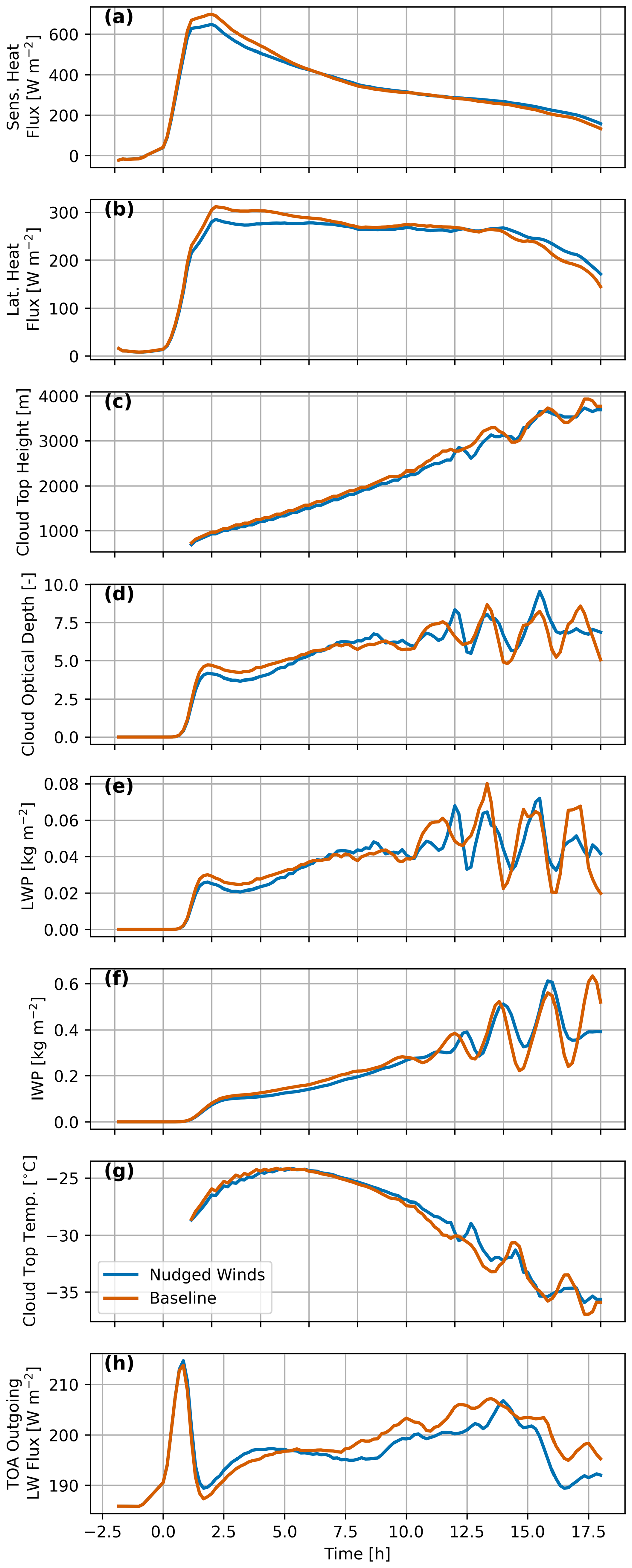
Here we briefly describe the sensitivity of the DHARMA model to a forcing using nudged versus geostrophic winds. Using a time constant of 30 min for nudging, we find better agreement with ERA5 wind speed and direction toward the end of the simulation (i.e., 18 h), while earlier times can deviate more strongly from ERA5 compared to a forcing using geostrophic winds, likely owing to local and sudden wind speed and direction fluctuations in ERA5 that are not represented in the derived geostrophic winds (not shown). When compared to a forcing with geostrophic winds, we find nudged winds to result in slightly smaller turbulent surface fluxes and cloud-top height during most of the simulation, which cloud condensate and radiative fluxes are largely insensitive to: during the first half of the simulation, we find a slight decrease in LWP, IWP, and cloud optical depth, resulting first in slightly larger outgoing TOA LW fluxes before slightly smaller ones in the second half of the simulation (Fig. A1). These results highlight a robustness of the forcing, with a preference for geostrophic winds for a more natural evolution (Sect. 2.2.2).

Figure A1 DHARMA LES output using geostrophic winds (labeled “baseline”) and nudged winds.

Appendix B: Sensitivity to physics options

Here we test additional model sensitivities to solar radiation, subsidence, and the treatment of the ice surface. These results used DHARMA with a 200 m grid cell spacing in the small domain configuration, with the model’s default roughness lengths.

The list of sensitivity tests, including a brief summary of the results, is as follows with legend names shown in Fig. B1 referred to in parentheses:

• DHARMA-MIZ-RAD_Lx25km_dx200_FixN (“Baseline”): We started with this more complex set-up. Upstream of the ice edge, the surface was treated as an ice surface of specified temperature and a fixed roughness length of $\mathrm{1.0}\times {\mathrm{10}}^{-\mathrm{4}}$ m. Downstream of the ice edge, Charnock’s relation was used for roughness over a water surface. Both shortwave (SW) and longwave radiation were included.

• DHARMA-MIZ-RAD_Lx25km_dx200_FixN_SWoff (“SW off”): Turning off SW radiation (ommited due to small effect).

• DHARMA-MIZ-RAD_Lx25km_dx200_FixN_SWoff_ Wsub (“SW off, subsidence”): Turning on large-scale subsidence derived from ERA5 (small effect as well). Given the fairly small subsidence values of this case, turning on subsidence only caused temporarily smaller cloud-top temperatures (∼1–2 K) and slightly greater IWP where cloud-top heights were briefly increased. Turning off subsidence avoided the need for offsetting specifications to avoid spurious thermodynamic evolution owing to the discontinuity at the domain top. Omitting subsidence also greatly simplifies analyses for process understanding.

• DHARMA-MIZ-RAD_Lx25km_dx200_FixN_noMIZ (“No MIZ”): Treating the ice surface as a water surface that is supercooled enough to match the sensible heat flux from the ice surface following Wu et al. (2025) also had little effect. This approach greatly simplifies the setup especially for Earth system model codes run in single-column model mode. Since it also had negligible effect that we could identify in LES, this was adopted as a helpful simplification.

We consider the differences between all of the simulations shown in Fig. B1 to be within the uncertainty of the specification derivation.

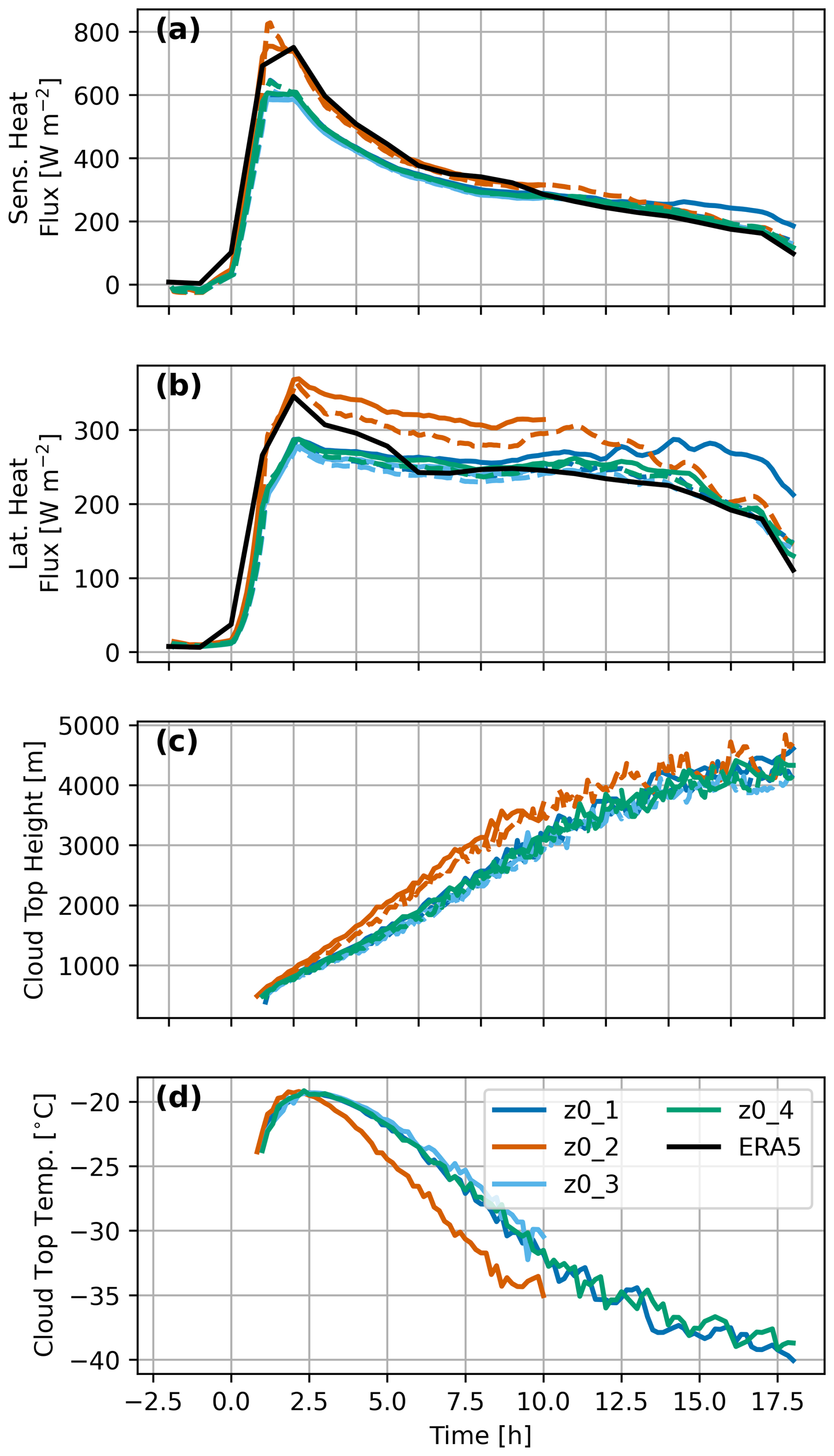
Figure B1 LES output using various surface roughness length configurations for DHARMA (solid lines) and WRF (dashed lines).

Appendix C: Sensitivity to roughness lengths

CAOs are inherently strongly surface-forced events. Therefore, we hypothesize that the roughness length formulations for momentum (z_0,m), temperature (z_0,t), and moisture (z_0,q) may notably impact CAO cloud evolution through surface momentum and heat fluxes. To test our hypothesis, we use WRF and DHARMA to test three sets of roughness length formulations and derive a reasonable set for COMBLE-MIP. While many formulations exist for z_0,m, z_0,t, and z_0,q, here we explore just a few of the more well-known formulations. For z_0,m, we use: $z_{\mathrm{0},\mathrm{m}}=a_{\mathrm{1}}\frac{u_{*}^{\mathrm{2}}}{g}+a_{\mathrm{2}}\frac{\mathit{\nu }}{u_{*}}$ where a₁=0.0154, a₂=0.11, u_* is friction velocity, g is acceleration due to gravity, and ν is kinematic viscosity. The functional form is based on Charnock (1955) and the value for a₂ comes from Smith (1988). The value for a₁ comes from COARE 3.5 (Edson et al., 2013, their Eq. 13, assuming a 10 m wind speed of 12 m s⁻¹). For the scalar roughness lengths (z_0,t and z_0,q), we use the functional form from Fairall et al. (2003, their Eq. 28): $z_{\mathrm{0},\mathrm{t},q}=min(\mathrm{1.1}\times {\mathrm{10}}^{-\mathrm{4}}$, $\mathrm{5.5}\times {\mathrm{10}}^{-\mathrm{5}}{R}_{\mathrm{r}}^{-\mathrm{0.6}})$ where R_r is the roughness Reynolds number, $R_{\mathrm{r}}=z_{\mathrm{0},\mathrm{m}}\frac{u_{*}^{\mathrm{2}}}{\mathit{\nu }}$.

We conduct four sensitivity simulations:

1. $z_{{\mathrm{0}}_{\mathrm{1}}}$: Compute z_0,m, z_0,t, and z_0,q according to above equations and constants.

2. $z_{{\mathrm{0}}_{\mathrm{2}}}$: Compute z_0,m according to above equations/constants and set $z_{\mathrm{0},\mathrm{t}}=z_{\mathrm{0},q}=\mathrm{0.1}{z}_{\mathrm{0},\mathrm{m}}$.

3. $z_{{\mathrm{0}}_{\mathrm{3}}}$: Set z_0,m, z_0,t, and z_0,q according to CONSTRAIN intercomparison case ($z_{\mathrm{0},\mathrm{m}}=\mathrm{6.6}\times {\mathrm{10}}^{-\mathrm{4}}$ m; $z_{\mathrm{0},\mathrm{t}}=z_{\mathrm{0},q}=\mathrm{3.7}\times {\mathrm{10}}^{-\mathrm{6}}$ m).

4. $z_{{\mathrm{0}}_{\mathrm{4}}}$: Compute constant z_0,m, z_0,t, and z_0,q values from $z_{{\mathrm{0}}_{\mathrm{1}}}$ for COMBLE-MIP case ($z_{\mathrm{0},\mathrm{m}}=\mathrm{9.0}\times {\mathrm{10}}^{-\mathrm{4}}$ m; $z_{\mathrm{0},\mathrm{t}}=z_{\mathrm{0},q}=\mathrm{5.5}\times {\mathrm{10}}^{-\mathrm{6}}$ m). [Note: DHARMA LES used $z_{\mathrm{0},\mathrm{t}}=z_{\mathrm{0},q}=\mathrm{5.0}\times {\mathrm{10}}^{-\mathrm{6}}$ m for this test.]

These results (Fig. C1) show clearly that the choice of roughness length parameterization can have a substantial impact on surface heat fluxes under the intense convective conditions during the 13 March CAO case (up to ∼20 %–30 % difference between $z_{{\mathrm{0}}_{\mathrm{2}}}$ and the other runs). In turn, the enhanced surface heat fluxes in $z_{{\mathrm{0}}_{\mathrm{2}}}$ lead to larger domain-averaged LWP and IWP values, with perhaps larger cells (as suggested by the greater fluctuations in values). Although, we cannot confidently say whether this is true because these simulations were conducted on a limited domain size. Additionally, the assumption of $z_{\mathrm{0},\mathrm{t}}=z_{\mathrm{0},q}=\mathrm{0.1}{z}_{\mathrm{0},\mathrm{m}}$ may be unreasonable in this case, as $z_{{\mathrm{0}}_{\mathrm{1}}}$ suggests much smaller z_0,t and z_0,q values. However, lack of observations prevents us from coming to a conclusion on this topic. We conclude that the fixed roughness lengths, which are used in $z_{{\mathrm{0}}_{\mathrm{4}}}$, are reasonable approximations for those derived from $z_{{\mathrm{0}}_{\mathrm{1}}}$, with relatively small differences apparent in the domain-mean kinematic, thermodynamic, and cloud fields.

Figure C1 DHARMA LES output using various physics options.

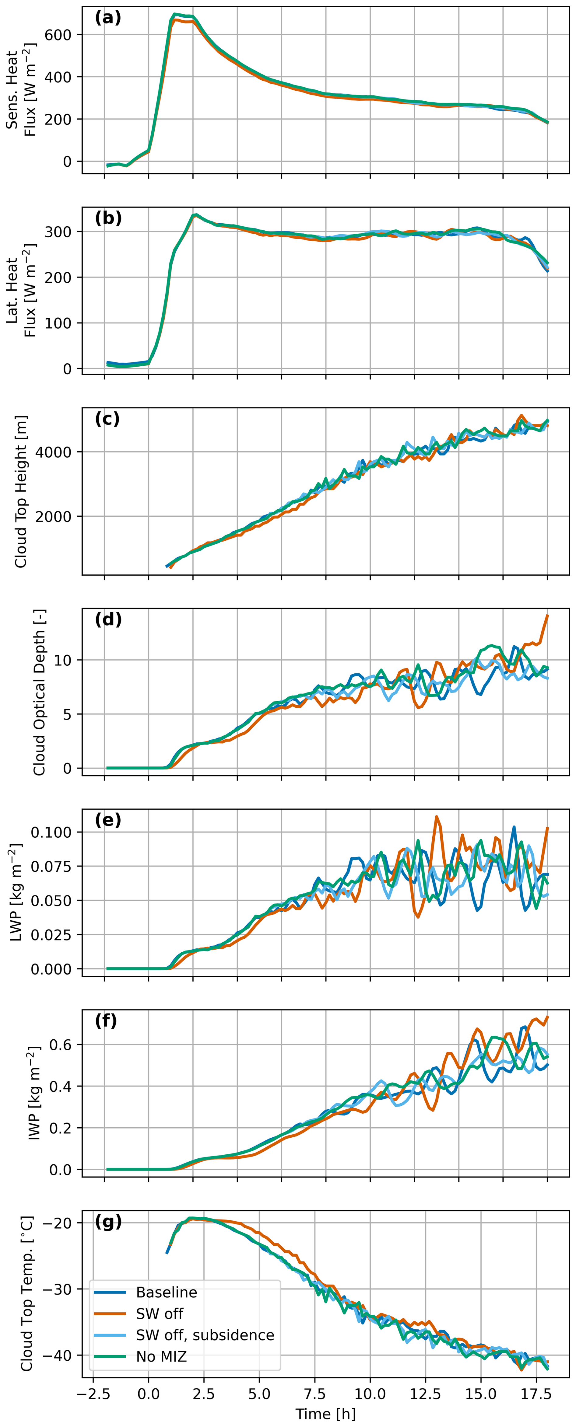
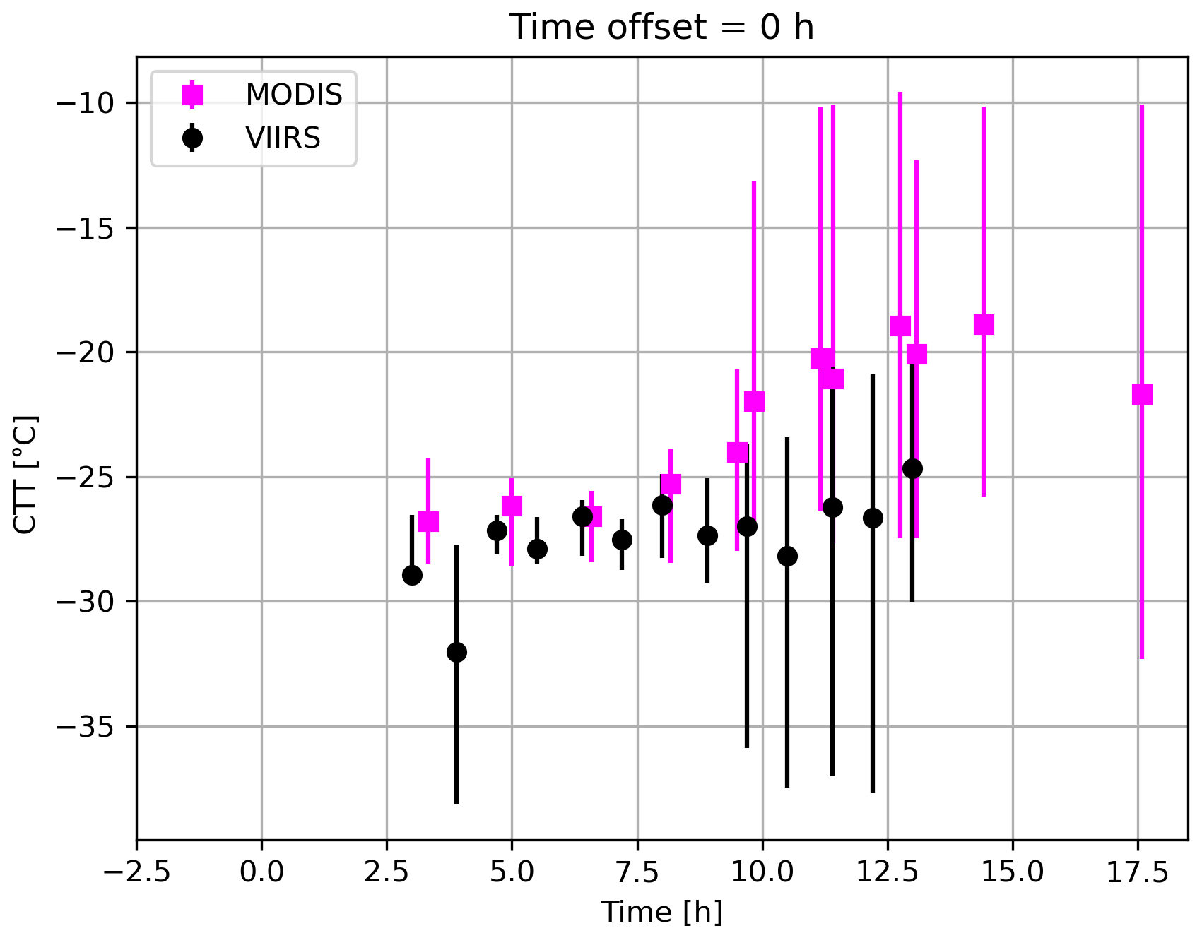
Figure C2 MODIS and VIIRS collocated brightness temperatures to infer cloud-top temperature show signs of surface contamination, evidenced by the large uncertainty bars. Mean values and bars are greater for MODIS that has a larger pixel size compared to VIIRS.

Appendix D: Supplementary curtain plot analysis

Here we provide additional curtain plots that demonstrate cloud condensate, relative humidity, and temperature differences across liquid-only and mixed-phase simulations using exemplary models. The use of two models (i.e., DHARMA and CM1-P3) is needed as neither model provides all variables fully. Given the relatively uniform response to configurations across LES codes, these plots offer a general idea of scenario differences that somewhat differ between LES codes.

Compared to mixed-phase clouds, liquid-only simulations gain warm-phase condensate (Fig. D1a–c) at the expense of frozen one (Fig. D1e–f). As a result, we find relative humidity with respect to liquid to increase inside the cloud layer and decrease below cloud (Fig. D1g–i). This relative humidity response is largely explained by changes in potential temperature that decreases inside the cloud and increases below cloud (Fig. D1j–l). The in-cloud response is partially caused by increased LW cooling near cloud-top (Fig. D1m–o) and decreased microphysical latent heat release (Fig. D1p–r). Below cloud, the liquid-only simulation shows smaller microphysical latent heat absorption (from decreased hydrometeor evaporation) compared to the mixed-phase simulation (where sublimation acts), resulting overall in greater sub-cloud temperature tendencies in liquid-only simulations. Section 3.2 examines all LES and SCM codes more widely.

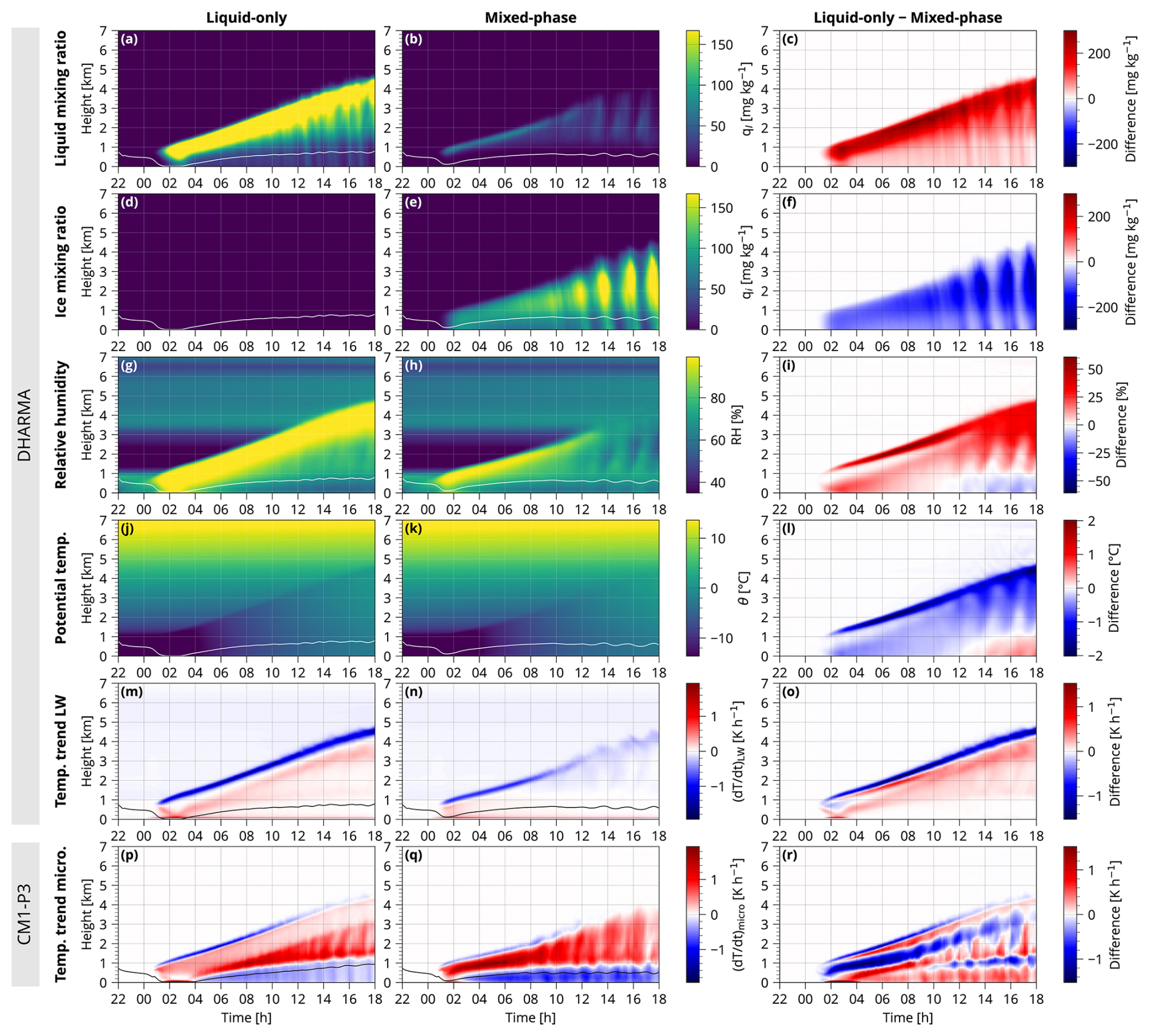
Figure D1 Curtain plots of liquid and ice mixing ratios (cloud plus precipitation), relative humidity (relative to liquid), potential temperature, temperature trend due to longwave radiation, and temperature trend due to microphysics in the DHARMA and CM1-P3 simulations for the liquid-only case, mixed-phase case, and their difference. The white and black lines show the lifting condensation level.