Do GEMS geostationary satellite observations of tropospheric NO₂ always improve NO_x emission estimates and related air quality modelling?

Satellite observations of atmospheric composition from low Earth orbit (LEO) have significantly advanced our understanding of global tropospheric chemistry; however, their 12 h overpass cadence limits the attribution of rapid compositional changes. The launch of the Korean Geostationary Environment Monitoring Spectrometer (GEMS) in 2020 heralded the beginning of continuous spaceborne monitoring of atmospheric composition during sunlit hours across Asia, allowing researchers to track atmospheric variability in real-time from a geostationary perspective. We assess the added value of GEMS observations of tropospheric NO₂ to estimate monthly NO_x emissions across Asia compared with the information provided by the equivalent instrument in LEO. We use the adjoint of the GEOS-Chem atmospheric chemistry transport model to infer NO_x emissions, comparing estimates using the full set of GEMS tropospheric NO₂ data against a surrogate LEO dataset created by subsampling the GEMS data at 13:45 local time (Korea Standard Time). We find that the benefits of assimilating high-frequency GEMS observations are most significant during non-summer months (September–May), when elevated NO₂ concentrations provide strong constraints on emission estimates. During this period, anthropogenic NO_x emission estimates derived from the full GEMS record deviate from LEO-proxy results, with differences of 0.2–52.6 Gg N per month, corresponding to 0.02 %–5.06 % of the a priori emissions. These differences further propagate into widespread adjustments in modelled ozone, hydroxyl radicals, and other secondary species, with evaluation against independent in situ measurements showing that GEMS-inferred emission estimates offer comparable or superior performance particularly in regions where the differences are most pronounced. In contrast, we find that during summer months (June–August), low NO₂ levels for which a larger fraction originates from lightning and other background sources with greater uncertainties likely challenge our 4D-Var framework, leading to negligible or even detrimental impacts on our ability to estimate NO_x emissions.

1 Introduction

Widespread anthropogenic pollutant emissions pose a severe threat to public health across Asia, a region home to approximately 4.78 billion people – roughly 60 % of the global population (Our World in Data, 2023). Effective air quality (AQ) management and mitigation strategies rely on the timely and accurate monitoring of these pollutant emissions. While conventional bottom-up inventories provide essential source-specific detail (Crippa et al., 2018; Hoesly et al., 2018; McDuffie et al., 2020; Crippa et al., 2023; Wang et al., 2024; Ekaterina and Li, 2024; Li et al., 2025), they are often hindered by reporting lags due to the labour-intensive nature of data collection. Top-down approaches, specifically satellite-based inverse modelling, offer a critical complementary framework by inferring emissions from real-time atmospheric observations (Wang et al., 2012; Xu et al., 2013; Wang et al., 2016, 2020; Cao et al., 2020). By integrating these two perspectives, researchers can generate the timely, actionable insights necessary for robust policy development and emission trend analysis.

Various spaceborne sensors provide the top-down observations necessary to constrain pollutant emission estimates through mathematical inverse modelling. Key instruments include the Moderate Resolution Imaging Spectroradiometer (MODIS) and the Multi-angle Imaging SpectroRadiometer (MISR) for aerosols (Wang et al., 2012; Xu et al., 2013); the Ozone Monitoring Instrument (OMI) and the Ozone Mapping and Profiler Suite (OMPS) for ozone (O₃), sulphur dioxide (SO₂), and nitrogen dioxide (NO₂) (Wang et al., 2016, 2020); and the Cross-track Infrared Sounder (CrIS) for ammonia (NH₃) (Cao et al., 2020). While newer platforms like the TROPOspheric Monitoring Instrument (TROPOMI) offer enhanced global distributions at higher spatial resolutions (Veefkind et al., 2012), these instruments are exclusively situated in low Earth orbit (LEO). This orbital configuration typically limits observations to two daily overpasses, roughly 12 h apart. For sensors dependent on solar backscatter, only the daytime pass is viable, a window often further obscured by cloud cover. This restricted temporal sampling creates a critical data gap, hampering our ability to resolve diurnal cycles and accurately attribute pollutant variability to specific emission sources or meteorological processes.

Geostationary Earth orbit (GEO) instruments address the temporal limitations of LEO platforms by providing high-frequency, continuous observations of a fixed region, typically at sub-hourly intervals during sunlit hours. While this capability has been foundational to meteorological monitoring and aerosol science, facilitated by instruments such as the Geostationary Ocean Color Imager (GOCI) and the Advanced Himawari Imager (AHI) (Xu et al., 2015; Yeom et al., 2020; Letu et al., 2020; Choi et al., 2023), it has recently expanded to encompass a broader suite of trace gases. The 2020 launch of South Korea’s Geostationary Environment Monitoring Spectrometer (GEMS) marked the advent of continuous spaceborne air quality monitoring (Choi et al., 2018; Kim et al., 2020). Combined with NASA's Tropospheric Emissions: Monitoring of Pollution (TEMPO) (Zoogman et al., 2017), launched in April 2023, and the European Space Agency's Sentinel-4 (Gulde et al., 2017), launched in July 2025, these sensors constitute the GEO AQ constellation. This international effort is expected to revolutionise our understanding of AQ variability and its underlying drivers, particularly over the densely populated regions of Asia, North America, and Europe.

As the first instrument of the GEO AQ constellation, GEMS provides hourly columnar loadings of O₃, aerosols, and key precursors (NO₂, SO₂, formaldehyde (HCHO), and glyoxal (CHOCHO)) at a high spatial resolution of a few km. Despite the substantial volume of data accumulated since 2020, existing literature has focused predominantly on retrieval algorithms and validation (Kim et al., 2023; Lee et al., 2024; Seo et al., 2024), as well as the characterization of diurnal cycles (Yang et al., 2024; Edwards et al., 2024). The use of these data for top-down emission estimates remains under-explored. Early efforts by Xu et al. (2023) used an empirical approach for point sources that bypassed complex atmospheric processing. More recently, Park et al. (2024, 2025) employed a Bayesian framework to infer Asian NO_x emissions, but their analysis was restricted to the winter–spring season of 2022 and species directly linked to NO_x. Consequently, it remains unclear how well geostationary NO₂ observations can infer NO_x emission estimates and subsequent atmospheric chemistry, specifically O₃ and aerosols, across a full annual cycle and varying seasonal photochemical regimes.

In this study, we quantify the added value of GEMS geostationary satellite observations of tropospheric NO₂ for constraining monthly NO_x emissions and to examine how this added value broadly influences our ability to model seasonal air pollutant distributions across the pan-Asian region from December 2020 to November 2021. We use the adjoint of the GEOS-Chem atmospheric chemistry transport model to infer NO_x emissions from the full set of GEMS tropospheric NO₂ data and a temporal subsample of that data at 13:45 local time (Korea Standard Time, KST) to represent a surrogate of LEO data. We use the latest GEMS v3.0 tropospheric NO₂ product, which incorporates corrected GEOS-Chem vertical coordinates for NO₂ shape factor calculations, resolving an issue identified in the previous v2.0 release (Oak et al., 2024). We analyse the spatiotemporal discrepancies and magnitude shifts between the two sets of inferred NO_x emissions, with particular emphasis on the anthropogenic component, and examine how these differences propagate across modelled atmospheric constituents, including NO₂, O₃, hydroxyl radicals (OH), carbon monoxide (CO), HCHO, SO₂, NH₃, and secondary inorganic aerosols (sulfate, nitrate, and ammonium). To validate the quantified added value of the geostationary observations, these modelled concentrations are benchmarked against independent in situ measurements.

The remainder of this paper is organized as follows: Section 2 details the GEOS-Chem adjoint model and the multi-source in situ datasets used for evaluation. Section 3 presents the inversion results for both the full GEMS dataset and the LEO proxy, evaluates their comparative performance, and discusses the implications for air quality modelling. Finally, Sect. 4 summarizes our findings in the context of previous studies and outlines future directions for GEMS data in atmospheric research.

2 Data and Methods

We first describe the GEMS v3.0 tropospheric NO₂ column data that we assimilate into the GEOS-Chem four-dimensional variational (4D-Var) data assimilation framework, including data screening and the characterization of error covariances. We then outline the 4D-Var framework and the experimental design that we have developed to quantify the added value of GEMS's high-frequency hourly sampling on emission constraints. Finally, we describe the suite of independent in situ measurements that we collected and used to evaluate the resulting chemical fields across the pan-Asian domain.

2.1 GEMS tropospheric NO₂ data as constraints

We use GEMS v3.0 Level-2 tropospheric NO₂ columns to infer monthly NO_x emissions over the pan-Asian region (50–160° E, 10° S–55° N) from December 2020 to November 2021. Although the model domain extends beyond the GEMS field of view (75–145° E, 5° S–45° N), atmospheric transport allows these observations to infer emission estimates both within and proximal to the satellite's footprint (Fig. S1 in the Supplement). As the first geostationary spectrometer of its kind, GEMS provides high-resolution hyperspectral measurements (300–500 nm; 0.6 nm full width half maximum) that enable the retrieval of multiple trace gases via Differential Optical Absorption Spectroscopy (DOAS) (Choi et al., 2018; Kim et al., 2020). This study focuses on NO₂ due to its direct link to NO_x emissions and its impacts on public health, both directly and indirectly through O₃ and aerosols (Yang et al., 2024; Luo et al., 2025), while establishing a framework for future multi-species chemical data assimilation. As its v3.0 quality flags are still maturing, we found that restricting the inversion to “best-quality” flags (flag = 0) was overly conservative. Following consultation with the GEMS team, we adopted a broader selection filter – Solar Zenith Angle <70°, Viewing Zenith Angle <70°, and Cloud Fraction <0.3 – to retain a robust dataset of approximately two billion retrievals. Data density peaks between 09:45 and 14:45 local time (KST) and during the warm season (April–September), reflecting optimal solar geometry and longer daylight hours (Fig. S2). Spatially, retrieval frequency is highest in the southeastern portion of the domain (Figs. S3, S4).

In addition to tropospheric NO₂ column densities, the assimilation process requires two critical parameters: retrieval uncertainties and averaging kernels. The former characterises the observational error budget, while the latter describes the vertical sensitivity of the GEMS instrument to the true NO₂ profile.

The GEMS product includes a unitless “RootMeanSquareError” variable; however, this only captures the DOAS fitting error and does not represent the total observational uncertainty. We thus follow the methodology of Yang et al. (2013, 2014) and Wang et al. (2020) to estimate the total uncertainty based on the standard deviation of retrievals within a pristine, pollution-free reference region. Although recommended by Boersma et al. (2007); Zara et al. (2018); Seo et al. (2024), the tropical Pacific (80–130° E, 5° S–5° N) can be influenced by seasonal biomass burning from Southeast Asia (Marvin et al., 2021, 2024); therefore, we identify a stable reference region (100–120° E, 20–30° N; Fig. S1) that is less influenced by major emission sources. The resulting estimated uncertainty of 0.0107 DU is comparable to the 0.011 DU reported for OMPS Level-2 data by Wang et al. (2020). While we acknowledge that pixel-level errors vary with cloud fraction, geometry, and aerosol loading, we adopt a uniform observation error of 0.0107 DU in the absence of analytical pixel-level estimates. To account for the uneven spatial distribution of GEMS observations (Figs. S3, S4), we scale this uncertainty by the square root of the number of valid observations per model grid cell on a monthly basis (Wang et al., 2020). This adjustment ensures a spatially balanced cost function within the GEOS-Chem 4D-Var framework, as detailed in Sect. 2.2.

Regarding vertical sensitivity, the GEMS NO₂ product provides a 47-layer averaging kernel (a), spanning the surface to 0.01 hPa. For our study, the troposphere is defined by layers below 230 hPa. The averaging kernel normalizes the scattering weights (w) by the reported air mass factor (AMF) such that $a\left(z\right)=\mathit{w}\left(z\right)/\text{AMF}$, where z represents the vertical layer index. Following Fu et al. (2025), we interpolate the modelled NO₂ profiles to the GEMS vertical grid (x_comp) and apply the kernels to derive a model-equivalent tropospheric column ($c_{\mathrm{comp}}^{\prime }$) that is directly comparable to the GEMS retrieval:

$$\begin{array}{}\text{(1)}& c_{\mathrm{comp}}^{\prime }=\sum _z\mathit{a}\left(z\right)\times {\mathit{x}}_{\mathrm{comp}}\left(z\right),\end{array}$$

where z goes from the surface to the tropopause. We note that this process differs from the application of the MOPITT and similar averaging kernels (Deeter, 2002). This is because the DOAS method retrieves a vertical column, whereas MOPITT and similar instruments retrieve vertical profiles using a Bayesian optimal estimation framework. Consequently, there is no need, nor is it possible, to introduce an additional term representing the difference between the retrieved and a priori profiles.

2.2 The GEOS-Chem model and its adjoint

The GEOS-Chem model (Bey et al., 2001) is a global 3-D chemical transport model driven by assimilated meteorological fields from the Goddard Earth Observing System (GEOS) of the NASA Global Modeling and Assimilation Office (GMAO). The GEOS-Chem adjoint model extends this forward simulation, providing a computationally efficient platform for calculating the sensitivity of a scalar cost function to a vast suite of model parameters (e.g., emissions) within a single backward integration (Henze et al., 2007, 2009). While these sensitivities can be used for direct sensitivity analysis, they are most often used within a 4D-Var data assimilation framework to optimize emission estimates, provided that the cost function is properly defined. To rigorously assess the added value of GEMS geostationary tropospheric NO₂ observations for monthly NO_x emission constraints and subsequent air quality modelling, we define the cost function (J) to be minimized as follows:

$$\begin{array}{}\text{(2)}& \begin{array}{rl}J& ={\displaystyle \frac{\mathrm{1}}{\mathrm{2}}}\sum _{\mathit{c}\in \mathbf{\Omega }}{\left(\mathbf{H}\mathit{c}-{\mathit{c}}_{\mathrm{obs}}\right)}^T{\mathbf{S}}_{\mathrm{obs}}^{-\mathrm{1}}\left(\mathbf{H}\mathit{c}-{\mathit{c}}_{\mathrm{obs}}\right)\\ & +{\displaystyle \frac{\mathrm{1}}{\mathrm{2}}}{\mathit{\gamma }}_{\mathrm{r}}{\left(\mathit{\sigma }-{\mathit{\sigma }}_{\mathrm{a}}\right)}^T{\mathbf{S}}_{\mathrm{a}}^{-\mathrm{1}}\left(\mathit{\sigma }-{\mathit{\sigma }}_{\mathrm{a}}\right),\end{array}\end{array}$$

where c is the vector of $c_{\mathrm{comp}}^{\prime }$ mapped to the observation space by the observation operator H; c_obs is the vector of GEMS tropospheric NO₂ retrievals; S_obs is the observation error covariance matrix; Ω is the spatiotemporal domain over which modelled and observed tropospheric NO₂ are compared; $\mathit{\sigma }=\ln (\mathit{E}\oslash {\mathit{E}}_{\mathrm{a}})$ is the vector of logarithmic scaling factors for the monthly NO_x emissions, on which sensitivities are calculated and which are optimized by the quasi-Newton L-BFGS-B algorithm (Byrd et al., 1995), with E and E_a denoting the a priori and a posteriori monthly NO_x emissions, respectively; σ_a is the prior estimate of the parameter scaling factors (set to zero in this study, meaning that our initial guess for E equals E_a); S_a is the error covariance estimate of the parameter scaling factors; and γ_r is a regularization parameter that balances the relative weights of the observation and penalty terms in the cost function.

For each GEMS tropospheric NO₂ retrieval within the spatiotemporal domain Ω, spanning the pan-Asian region for each month from December 2020 to November 2021, the observation operator H identifies the corresponding model grid cell. The modelled value is then adjusted using the averaging kernels at the assimilation time step most proximal to the retrieval time. We assume the observation error covariance matrix, S_obs, is diagonal; the diagonal elements represent the total estimated uncertainty, scaled by observation density as detailed in Sect. 2.1, while the off-diagonal elements are set to zero, assuming spatially uncorrelated observation errors. The specification of the a priori error covariance matrix, S_a, is contingent upon the emission inventories employed. Although recent versions of the GEOS-Chem forward model support a diverse array of state-of-the-science inventories, the adjoint model supports a more restricted subset. While 4D-Var inversions are primarily constrained by atmospheric observations and are thus less sensitive to the initial a priori selection, utilizing contemporary emission inventories remains preferable to facilitate superior convergence during the optimization process (Tang et al., 2023). Following the implementation of aromatic chemistry and a suite of contemporary emission inventories into the GEOS-Chem adjoint by Wang et al. (2021), we extend those inventories to align with our study period. Anthropogenic emissions for China are derived from the Multi-resolution Emission Inventory for China (MEIC), updated to 2020 (Zheng et al., 2018, 2021), while the MIX-Asia inventory (Li et al., 2017) is applied to the remainder of the Asian domain. Global anthropogenic emissions outside of Asia are taken from the Community Emissions Data System (CEDS) (Hoesly et al., 2018). Biomass burning emissions are sourced from the Global Fire Emissions Database version 4.1 (GFED4s) (van Der Werf et al., 2017), extended through 2021. Natural NO_x precursors, including lightning (Price and Rind, 1992), soil (Yienger and Levy, 1995), and biogenic sources (Guenther et al., 2012), are calculated online within the GEOS-Chem framework. We assign an a priori uncertainty of 40 % to anthropogenic emissions, representing a 2020 emission-weighted average of the uncertainties reported for MEIC and MIX-Asia (Li et al., 2017; Zheng et al., 2018). For non-anthropogenic emissions, we assign a broader uncertainty of 100 %, consistent with previous inverse modeling studies across the pan-Asian region (Xu et al., 2013; Wang et al., 2020; Souri et al., 2020; Jung et al., 2022; Park et al., 2023, 2024, 2025). The a priori error covariance matrix, S_a, is also assumed to be diagonal. This neglects spatial error correlations, a simplification justified by the fact that the correlation length scales of individual emission sources are typically smaller than the model's grid resolution (Stephen and Aneja, 2008). To further mitigate potential adverse effects of neglecting error correlations, we apply a regularization parameter (γ_r) to enforce a smoother solution. We set γ_r to 10, a value identified as optimal through L-curve analysis in similar 4D-Var applications (Hansen, 1998; Henze et al., 2009).

While we acknowledge that the specifications for S_obs, S_a, and γ_r entail inherent uncertainties, a comprehensive parameter sensitivity analysis is beyond the scope of this work. Instead, this study focuses on a relative assessment of the added value provided by geostationary sampling. By maintaining consistent parameter settings across our experimental suite, the contrast between inversions serves as a controlled metric for evaluating the impact of high-frequency observations. We distinguish between two primary experiments: a “GEMS-based” inversion using the full hourly dataset and a “LEO-proxy” inversion that serves as a surrogate for LEO instruments (e.g., OMI, OMPS, TROPOMI) by sub-setting observations to 13:45 local time (KST). Specifically, the “GEMS-based” inversion ingests all GK2_GEMS_L2_YYYYMMDD_hhmm_NO2_[Scan area]_DPRO_ORI.nc files, whereas the “LEO-proxy” inversion ingests only those with hhmm = 00:45 UTC (13:45 KST). For both cases, the cost function is minimized over ten iterations; we found that further iterations yielded marginal improvements, thus ten iterations represent an optimal balance between computational efficiency and convergence accuracy. The simulations are conducted at a global horizontal resolution of 2° × 2.5° with 47 vertical layers, driven by GEOS-FP meteorological fields (1 h temporal resolution for 2-D fields; 3 h for 3-D fields) (Lucchesi, 2013). While nested-grid simulations at 0.25° × 0.3125° are possible for sub-regions like China, the 2° × 2.5° resolution was selected to ensure computational feasibility across the entire pan-Asian domain. Initial conditions were established via a long-term spin-up starting in January 2019 to eliminate the influence of initial state concentrations on the inversion results.

Following the updates to the GEOS-Chem adjoint framework, we perform a dual-phase evaluation of the model's performance. First, we execute a localized gradient consistency test by disabling horizontal transport processes. Under this configuration, the sensitivity of the observational cost function (excluding the regularization term) within an individual grid cell with respect to the local emission scaling factor (σ) becomes mathematically equivalent to the total sensitivity across the entire domain. This simplification allows for a direct, grid-by-grid comparison between sensitivities derived from the adjoint method and those calculated via the finite difference method. We verify the numerical accuracy of the adjoint-based gradients by using the finite difference results as a benchmark:

$$\begin{array}{}\text{(3)}& \wedge ={\displaystyle \frac{J_{\mathrm{obs}}(\mathit{\sigma }+\mathit{\delta }\mathit{\sigma })-J_{\mathrm{obs}}(\mathit{\sigma }-\mathit{\delta }\mathit{\sigma })}{\mathrm{2}\mathit{\delta }\mathit{\sigma }}},\end{array}$$

where J_obs is the observation part of the cost function. We adopt a perturbation of δσ=0.01 to calculate the finite-difference gradients, a value found to optimally balance truncation and round-off errors (Henze et al., 2009).

Second, we evaluate the internal consistency of the inversion by comparing modelled tropospheric NO₂ columns against the GEMS retrievals both before (a priori) and after (a posteriori) the optimization. While this assessment is not independent of the assimilation process, it serves as a critical diagnostic to verify that the 4D-Var framework effectively minimizes the model-observation mismatch and that the adjoint system is functioning as intended.

2.3 Experimental design

To reiterate, we conduct two distinct 4D-Var inversion experiments for each month from December 2020 to November 2021 across the pan-Asian region to rigorously quantify the added value of geostationary sampling for monthly NO_x emission constraints and subsequent air quality modelling:

• GEMS-based inversion. This experiment assimilates the full temporal suite of GEMS tropospheric NO₂ retrievals, leveraging the high-frequency diurnal sampling inherent to geostationary observations.

• LEO-proxy inversion. This experiment utilizes a subset of GEMS retrievals restricted to 13:45 local time (KST). This serves as a surrogate for LEO instruments (e.g., TROPOMI, OMI, and OMPS) which provide only a single daily overpass.

Both inversions use identical a priori emissions, model configurations, and cost function parameter settings. The optimization is achieved through ten iterations of the forward and adjoint model integrations. We evaluate the impact of hourly sampling by comparing the spatiotemporal distribution and magnitude of the resulting a posteriori monthly NO_x emissions, with particular emphasis on the anthropogenic component. Furthermore, we examine the sensitivity of related chemical species, including O₃, OH, CO, HCHO, SO₂, NH₃, and secondary inorganic aerosols (sulfate, nitrate, and ammonium), to the different emission constraints. To validate the quantified added value of GEMS data, the modelled atmospheric constituents are evaluated against independent in situ measurements. Detailed descriptions of these independent datasets are provided below.

2.4 In situ measurements for independent assessment

To evaluate the chemical propagation of the monthly NO_x emissions inferred from the “GEMS-based” and “LEO-proxy” inversions, we employ a diverse suite of independent in situ measurements. Hourly measurements of surface concentrations of NO₂, O₃, CO, SO₂, NH₃, and fine and coarse particulate matter are obtained from four national monitoring networks: the China National Environmental Monitoring Center (CNEMC), AirKorea, the Japanese Environmental Observatory of the National Institute for Environmental Studies, and the Indian Central Pollution Control Board (CPCB). Due to varying reporting standards across these networks, modelled outputs are converted to the respective reported units and evaluated separately for each network. The spatial distribution of these surface monitoring stations is illustrated in Fig. S1. For vertical column validation, we use high-frequency measurements from the Aerosol Robotic Network (AERONET) and the Pandonia Global Network (PGN). While AERONET is primarily recognized for aerosol characterization, it provides valuable columnar NO₂ and O₃ at intervals up to 15 min; 94 AERONET sites are available within our domain (Fig. S1). We complement these data with columnar NO₂ from seven PGN sites, which offer sampling frequencies as high as every 2 min. To ensure data robustness and computational efficiency, we retain only PGN retrievals with the highest quality flag (flag = 0) and aggregate them into hourly averages for comparison with the model.

To rigorously evaluate the modelled atmospheric constituents against in situ measurements, we sample the model at the exact time and location of each observation. Although the “GEMS-based” and “LEO-proxy” inversions only update monthly NO_x emissions, these updates are spatially heterogeneous and therefore exert non-uniform impacts on the modelled atmospheric constituents across both space and time. We thus compile the paired data into GEOS-Chem grid composites at multiple temporal scales to assess the model performance driven by the two sets of inferred NO_x emissions. The temporal scales include the afternoon at 13:45 local time (KST), daytime averages (07:45 to 16:45 KST), and full daily averages. The first two correspond to the overpass periods represented by the “LEO-proxy” and “GEMS-based” inversions. This multi-temporal approach enables us to assess how the assimilated observations influence model performance both during the outside the observation periods. To quantify the agreement between modelled and measured values, we employ a suite of geometrically related statistical metrics, including the Pearson correlation coefficient (R), normalised standard deviation (NSD), and normalised centralised root-mean-square error (NRMSE), defined as follows:

$$\begin{array}{}\text{(4)}& {\displaystyle }R={\displaystyle \frac{{\sum }_{i=\mathrm{1}}^N(M_i-\stackrel{\mathrm{‾}}{M})(O_i-\stackrel{\mathrm{‾}}{O})}{\sqrt{{\sum }_{i=\mathrm{1}}^N(M_i-\stackrel{\mathrm{‾}}{M}{)}^{\mathrm{2}}}\sqrt{{\sum }_{i=\mathrm{1}}^N(O_i-\stackrel{\mathrm{‾}}{O}{)}^{\mathrm{2}}}}},\text{(5)}& {\displaystyle }\mathrm{NSD}={\displaystyle \frac{\sqrt{\frac{\mathrm{1}}{N}{\sum }_{i=\mathrm{1}}^N(M_i-\stackrel{\mathrm{‾}}{M}{)}^{\mathrm{2}}}}{\sqrt{\frac{\mathrm{1}}{N}{\sum }_{i=\mathrm{1}}^N(O_i-\stackrel{\mathrm{‾}}{O}{)}^{\mathrm{2}}}}},\text{(6)}& {\displaystyle }\mathrm{NRMSE}={\displaystyle \frac{\sqrt{\frac{\mathrm{1}}{N}{\sum }_{i=\mathrm{1}}^N\left(\right(M_i-\stackrel{\mathrm{‾}}{M})-(O_i-\stackrel{\mathrm{‾}}{O}){)}^{\mathrm{2}}}}{\sqrt{\frac{\mathrm{1}}{N}{\sum }_{i=\mathrm{1}}^N(O_i-\stackrel{\mathrm{‾}}{O}{)}^{\mathrm{2}}}}},\end{array}$$

where M and O denote the modelled and measured values, respectively; $\stackrel{\mathrm{‾}}{M}$ and $\stackrel{\mathrm{‾}}{O}$ represent their respective means; and N is the total number of paired data. Collectively, these metrics provide a comprehensive evaluation of model performance: R captures the ability to reproduce temporal and/or spatial variability; NSD indicates the relative magnitude of modelled variability compared to the observations; and NRMSE quantifies the overall deviation, normalised by the measured variability. Following the geometric relationship ${\mathrm{NRMSE}}^{\mathrm{2}}=\mathrm{1}+{\mathrm{NSD}}^{\mathrm{2}}-\mathrm{2}\cdot \mathrm{NSD}\cdot R$, these three metrics can be jointly visualised in a Taylor diagram (Taylor, 2001). In this coordinate system, R is represented by the azimuthal angle, NSD by the radial distance from the origin, and NRMSE by the distance from the reference point (denoting perfect performance where R=1 and NSD=1). Such a diagram offers an intuitive and concise framework to summarise and compare our evaluation results across both inversions and multiple temporal scales.

The three metrics described above, however, do not capture the overall bias between modelled and measured values. We therefore additionally define and visualize the normalized mean bias (NMB) on the same Taylor diagram to complement the model evaluation:

$$\begin{array}{}\text{(7)}& \mathrm{NMB}={\displaystyle \frac{{\sum }_{i=\mathrm{1}}^N(M_i-O_i)}{{\sum }_{i=\mathrm{1}}^N{O}_i}}.\end{array}$$

From R and NSD, we further define an overall model skill metric (S) that combines both metrics as follows:

$$\begin{array}{}\text{(8)}& S={\displaystyle \frac{\mathrm{4}(\mathrm{1}+R)}{(\mathrm{NSD}+\mathrm{1}/\mathrm{NSD}{)}^{\mathrm{2}}(\mathrm{1}+R_{\mathrm{0}})}},\end{array}$$

where R₀ represents the maximum achievable correlation coefficient given measurement uncertainties; for the purposes of this study, R₀ is set to 1. The resulting model skill score, S, ranges from 0 to 1, where a value of 1 signifies perfect agreement between modelled and observed values. We present this metric in a bar chart positioned beneath each Taylor diagram; together, these visualisations facilitate a robust comparison of the model performance yielded by the “GEMS-based” and “LEO-proxy” inversions.

3 Results and Discussion

3.1 Evaluation of updates to the adjoint of GEOS-Chem model

We investigate the capacity of GEMS geostationary tropospheric NO₂ observations to enhance monthly NO_x emission estimates and subsequent air quality modelling across a full annual cycle (December 2020–November 2021). Our analysis reveals that the contrasts between the “GEMS-based” and “LEO-proxy” inversions primarily follow two distinct seasonal patterns: non-summer (September to May) and summer (June to August). To capture these patterns efficiently, we validate our adjoint model updates using two representative months: January and July 2021. For each representative month, we perform both a 6 h and a 1 d simulation. The 1 d simulation incorporates the full suite of GEMS retrievals, while the 6 h simulation subsets only those observations at 13:45 local time (KST) to serve as a LEO surrogate. This configuration ensures the validation conditions closely mirror the operational “GEMS-based” and “LEO-proxy” inversions. Figure 1 shows that the linear correlation coefficients and regression slopes between the adjoint-based and finite-difference-based sensitivities are nearly unity for both months and durations. These results verify the successful integration of contemporary emission inventories, aromatic chemistry, and new observation operators into the GEOS-Chem adjoint framework.

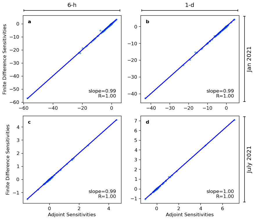
Figure 1 Evaluation of updates to the adjoint of GEOS–Chem model by comparing adjoint–based and finite–difference–based sensitivities of the cost function (penalty term is excluded, and horizontal transport is turned off) with respect to logarithmic scaling factors of anthropogenic NO_x emissions for January (a, b) and July (c, d) 2021 with a 6 h simulation including only GEMS tropospheric NO₂ retrievals at 13:45 local time (Korea Standard Time) (a, c) and with a 1 d simulation including all available GEMS tropospheric NO₂ retrievals for that day (b, d). The linear correlation coefficients (R) and linear regression slopes between the two sets of sensitivities are also shown in each panel.

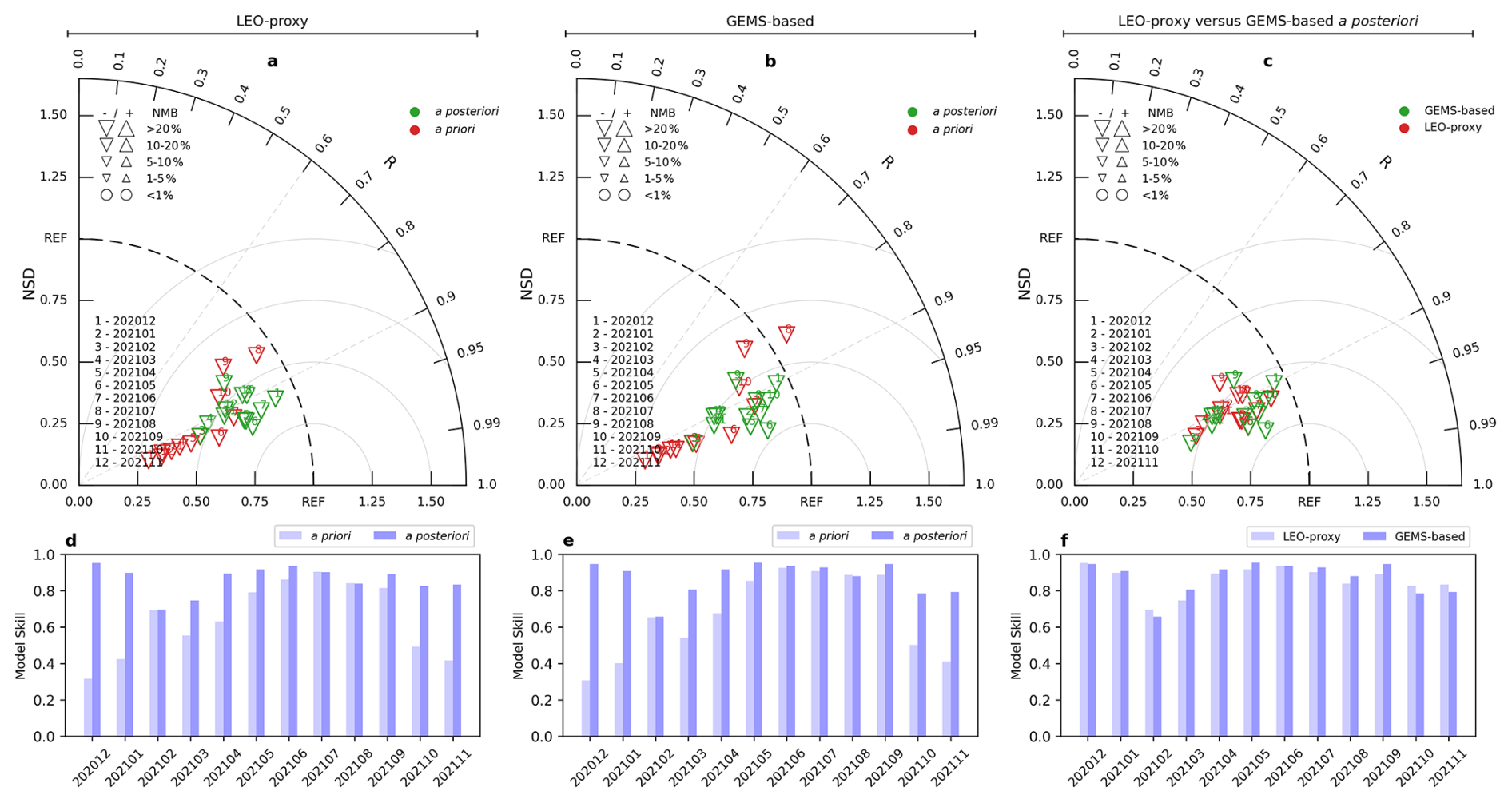
Figure 2 Non-independent model evaluation for the “LEO-proxy” (a, d) and “GEMS-based” (b, e) inversions, and a comparison between them (c, f). Each point on the taylor diagram (a–c) represents the Pearson correlation coefficient (R), normalized standard deviation (NSD), normalized centered root-mean-square error (NRMSE), and normalized mean bias (NMB) between modelled and satellite-retrieved tropospheric NO₂, which are interpreted by the azimuthal angle (R), radial distance from the origin (NSD), distance from the reference (REF) point (NRMSE), and the marker shape and size (NMB), respectively. The points distinguish between a priori (red) and a posteriori (green) model simulations in panels (a) and (b), as well as between the “LEO-proxy” (red) and “GEMS-based” (green) a posteriori simulations in panel (c). Each vertical bar in panels (d)–(f) shows the model skill before and after the “LEO-proxy” and “GEMS-based” inversions, as well as a comparison between their a posteriori model skill.

While accurate sensitivity computation is a prerequisite, the ultimate objective is the optimization of the logarithmic scaling factors of monthly NO_x emissions within the 4D-Var framework. Figure 2 presents an evaluation of the modelled tropospheric NO₂ columns against GEMS retrievals both before and after the optimisation. Although these evaluations are not independent, as the GEMS data are used for both constraint and evalution, they provide a necessary internal consistency check. We find that both inversions consistently reduce the model-observation mismatch across all months, with the most significant improvements observed during the non-summer (September to May) period. For instance, the overall model skill, S, has been improved by 0.47 %–208.65 % and 0.32 %–200.36 % during this period in the “GEMS-based” and “LEO-proxy” inversions, respectively. Despite the differing data densities between the “GEMS-based” and “LEO-proxy” experiments, the consistent performance enhancements demonstrate that the updated adjoint model effectively optimises emissions. This successful evaluation provides the foundation for our subsequent assessment of the added value of GEMS geostationary observations of tropospheric NO₂ for monthly NO_x emission constraints and related air quality modelling.

3.2 Overall model evaluation against independent in situ measurements

Here we present the comprehensive model evaluation results against independent measurements of both columnar and surface NO₂ obtained from the in situ datasets detailed in Sect. 2.4. To complement this overarching evaluation, independent model evaluation results for other chemical species within selected subregions are provided in Sect. 3.4. In that section, we further explore the contrasts in modelled atmospheric constituents between the “GEMS-based” and “LEO-proxy” inversions to quantify the added value of geostationary sampling.

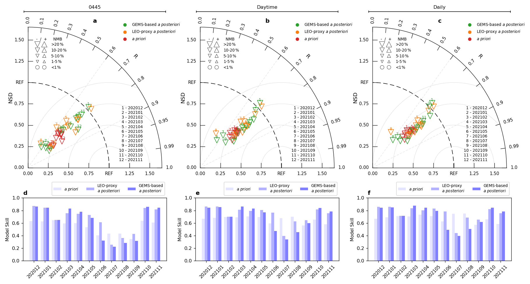
Figure 3 Independent model evaluation against columnar NO₂ measurements from the Aerosol Robotic Network (AERONET) for the “LEO-proxy” and “GEMS-based” inversions across multiple temporal scales, including the afternoon at 13:45 local time (Korea Standard Time, KST) (a, d), daytime averages (07:45 to 16:45 KST) (b, e), and full daily averages (c, f). The interpretation of the Taylor diagrams (a–c) and model skill bar charts (d–f) is the same as that described in the caption of Fig. 2, except that here we distinguish the a priori, “LEO-proxy” a posteriori, and “GEMS-based” a posteriori model simulations on each of the Taylor diagrams and model skill bar charts.

Figure 3 shows the independent model evaluation results against columnar NO₂ measurements from AERONET. We observe that during the non-summer months (September to May), both inversions yield substantial improvements over the a priori simulation across all investigated temporal scales, including afternoon, daytime, and daily averages. Crucially, the model performance driven by NO_x emissions from the “GEMS-based” inversion is generally superior or comparable to that of the “LEO-proxy” inversion. For instance, the largest improvements in the overall model skill, S, from the “LEO-proxy” inversion to the “GEMS-based” inversion occur in March or April, corresponding to 9.53 %, 6.09 %, and 5.02 % increases in the afternoon, daytime, and daily-average evaluations, respectively. Conversely, during the summer months (June to August), the performance of both inversions degrades relative to the a priori simulation. In this period, the “GEMS-based” inversion performs slightly worse than the “LEO-proxy” counterpart. This seasonal discrepancy is also reflected in the independent validation against PGN columnar NO₂ measurements (Fig. S5), although the limited number of PGN sites constrains the statistical robustness of these findings. To address this, we selected a specific site in Beijing characterised by high data coverage and more recent a priori emission data. The scatterplots of modelled versus measured columnar NO₂ at this site (Fig. S6) further corroborate the contrasting patterns between the non-summer and summer periods identified in the broader PGN dataset.

Figures S7 and S8 show the independent model evaluation results against surface NO₂ measurements from CNEMC and CPCB, respectively. Consistent with the columnar evaluation, we observe a seasonal divide in China: both inversions yield performance improvements during the non-summer months (September to May) but result in degradations during the summer months (June to August). Notably, the “GEMS-based” inversion exerts a more pronounced influence on the magnitude of these performance shifts compared to the “LEO-proxy” version. In contrast, model performance in India remains largely unchanged from the a priori simulation across all seasons and experiments. This lack of sensitivity is likely attributable to the lower density of GEMS tropospheric NO₂ retrievals over the Indian subcontinent relative to China (Figs. S3, S4). For both the CNEMC and CPCB datasets, the model demonstrates higher skill when evaluated against daytime and daily averages rather than specific afternoon values. This suggests that high-frequency hourly measurements, which are not quality-screened, may contain stochastic noise that is effectively smoothed through temporal averaging. Furthermore, the relatively coarse spatial resolution of the model (2° latitude × 2.5° longitude) likely contributes to this trend, as temporal averaging helps mitigate the spatial representativeness mismatch between point-based in situ measurements and grid-averaged model values.

Ideally, a direct comparison between GEMS tropospheric NO₂ retrievals and in situ measurements would help reveal the factors driving the observed model degradation during summer. However, such an analysis is precluded by the absence of the requisite averaging kernels for both datasets, preventing a mathematically consistent comparison. We therefore speculate that the reduced model performance during the summer months is partly attributable to the markedly lower values of GEMS tropospheric NO₂ columns in summer than in non-summer months (Figs. S9–S11), which are primarily due to enhanced photochemical losses under stronger solar radiation (Edwards et al., 2024; Seo et al., 2024). The low signal-to-noise ratios under low-NO₂ conditions likely make it more challenging for the 4D-Var inversion to effectively constrain monthly NO_x emissions. Additionally, during summer months lightning and other background sources likely contribute a larger fraction of these low tropospheric NO₂ columns, and their greater uncertainties than those of anthropogenic sources further complicate the inversion. The “GEMS-based” inversion assimilates a larger volume of observations with these characteristics, potentially explaining why it performs even more poorly than the “LEO-proxy” inversion, even though summertime exhibits much stronger diurnal variability (Fig. S12 versus S13). In this sense, at least for our 4D-Var framework, the magnitude of the tropospheric NO₂ columns appears to play a more important role in inversion performance than the additional diurnal information provided by geostationary sampling.

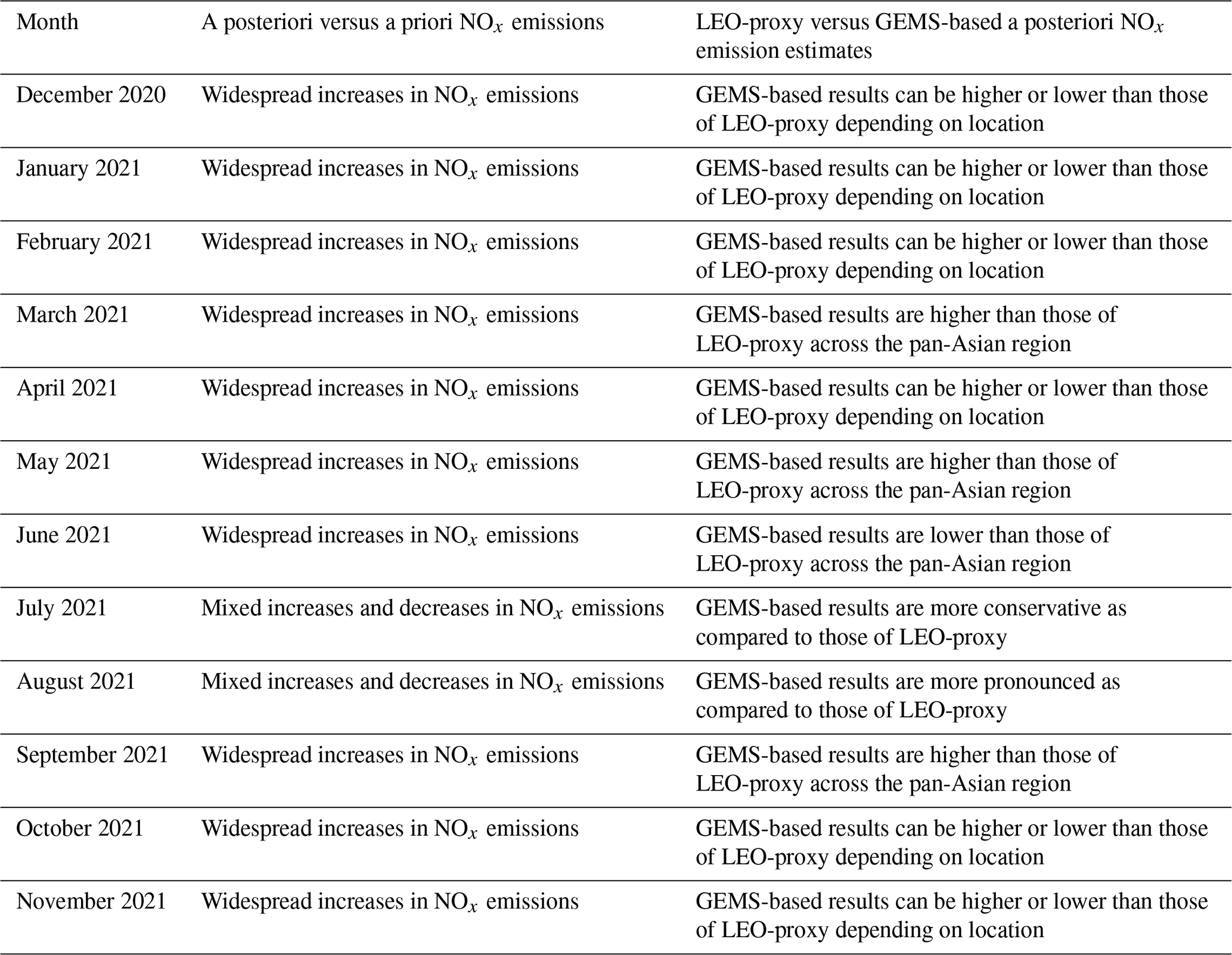
Table 1 Comparisons of the “LEO-proxy” and “GEMS-based” a posteriori NO_x emission estimates relative to the a priori NO_x emissions, along with a comparison between their a posteriori NO_x emission estimates.

3.3 Contrasts in inferred anthropogenic NO_x emissions between GEMS-based and LEO-proxy inversions

Table 1 provides a summary of the adjustments made to the a priori anthropogenic NO_x emissions by the “GEMS-based” and “LEO-proxy” inversions, alongside a comparison of their respective a posteriori estimates. The spatial distributions of these emission adjustments and the differences between the two inversions are presented in Figs. S14–S16. Focusing on the non-summer period (September to May), both inversions generally result in widespread increases in anthropogenic NO_x emissions. However, the magnitude of these adjustments varies spatially and temporally; the “GEMS-based” estimates are either higher or lower than the “LEO-proxy” values depending on the specific region and month. For instance, Figs. 4c1 and S17c show that in April 2021, the “GEMS-based” inversion produces higher anthropogenic NO_x emission estimates across much of North China Plain, whereas the inverse is true over Northern India. This spatial divergence largely mirrors the differences in the distribution of the full GEMS dataset compared to the 13:45 KST subset (Figs. 4c2 and S17i). This relationship is further confirmed by a statistically significant Pearson correlation coefficient (R=0.49) between the differences in a posteriori emissions and the differences in GEMS retrievals (Fig. 4c4). While the updates to a priori emissions primarily propagate linearly to modelled tropospheric NO₂ concentrations (Fig. 4a12 and b12), some non-linearities persist. Consequently, the differences in modelled NO₂ between the two experiments (Figs. 4c3 and S17f) also align with the retrieval differences, showing a strong correlation of R=0.71 (Fig. 4c4). Although we omit a detailed discussion for every non-summer month for the sake of brevity, the significant month-to-month variability underscores the necessity of performing independent monthly inversions, as the results of one cannot serve as a direct proxy for another.

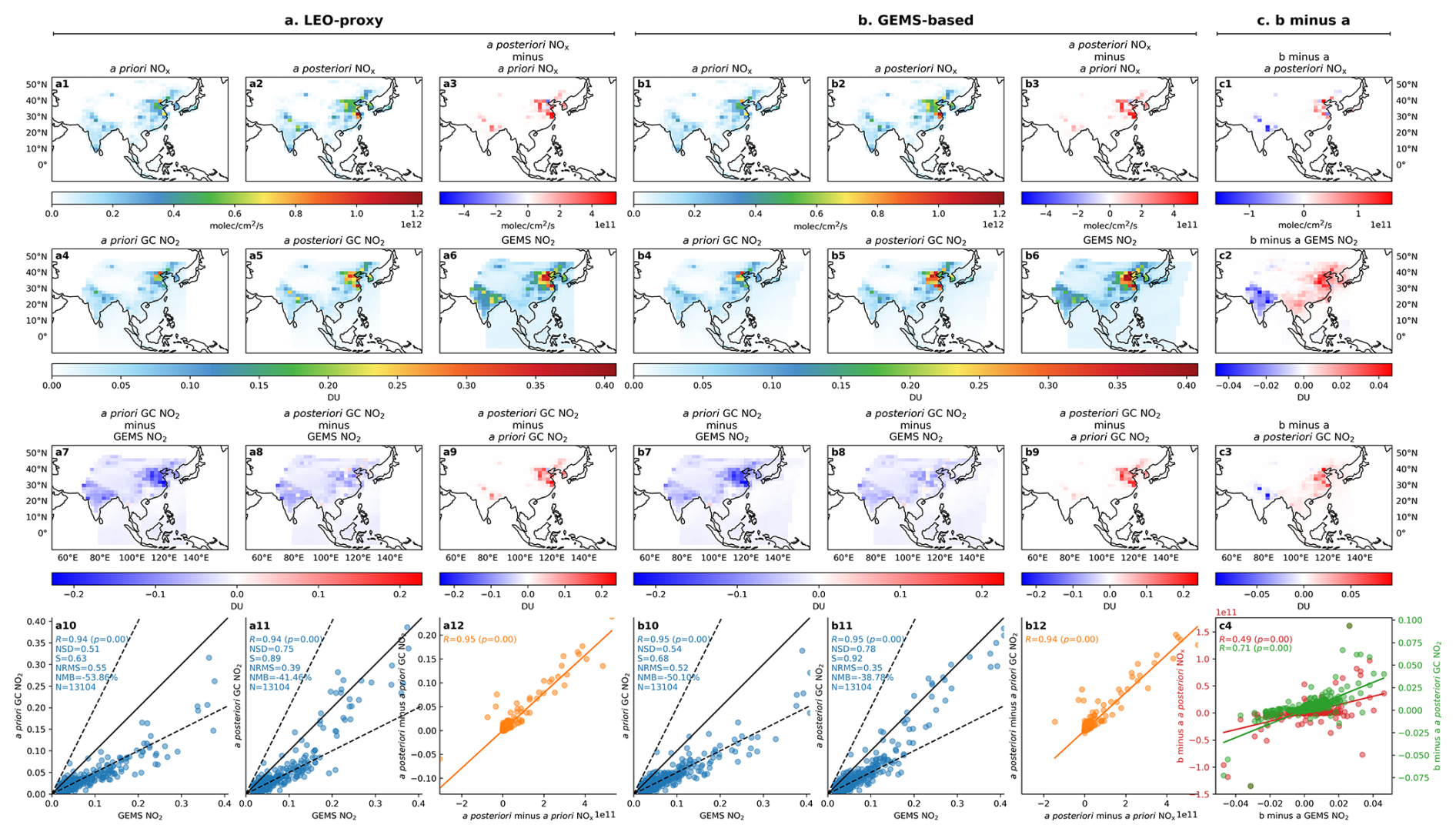
Figure 4 Results for April 2021 from the “LEO-proxy”(a1–a12) and “GEMS-based” (b1–b12) inversions, along with a comparison between them (c1–c4). For each inversion, we show: the a priori anthropogenic NO_x emissions (a1, b1) and a posteriori anthropogenic NO_x emissions (a2, b2), their differences (a3, b3), modelled tropospheric NO₂ based on the a priori (a4, b4) and a posteriori (a5, b5) emissions and the associated changes from a priori to a posteriori (a9, b9), the differences between modelled and GEMS tropospheric NO₂ (a6, b6) for a priori (a7, b7) and a posteriori (a8, b8) values, scatter plots of modelled versus GEMS tropospheric NO₂ for a priori (a10, b10) and a posteriori (a11, b11) values, and finally scatter plots of the differences between a posteriori and a priori modelled tropospheric NO₂ and NO_x (a12, b12). For comparing the two inversions, we show the differences between their a posteriori anthropogenic NO_x emissions (c1) and the subsequently modelled NO₂ (c3) alongside the corresponding GEMS tropospheric NO₂ (c2), as well as scatter plots of the differences in modelled tropospheric NO₂ and NO_x between the two inversions versus the corresponding differences in GEMS tropospheric NO₂ retrievals (c4). For panels (a3), (b3), (c1), (a9), (b9), (c3), (a8), (b8), (c2), we show their respective percentage changes in Fig. S17.

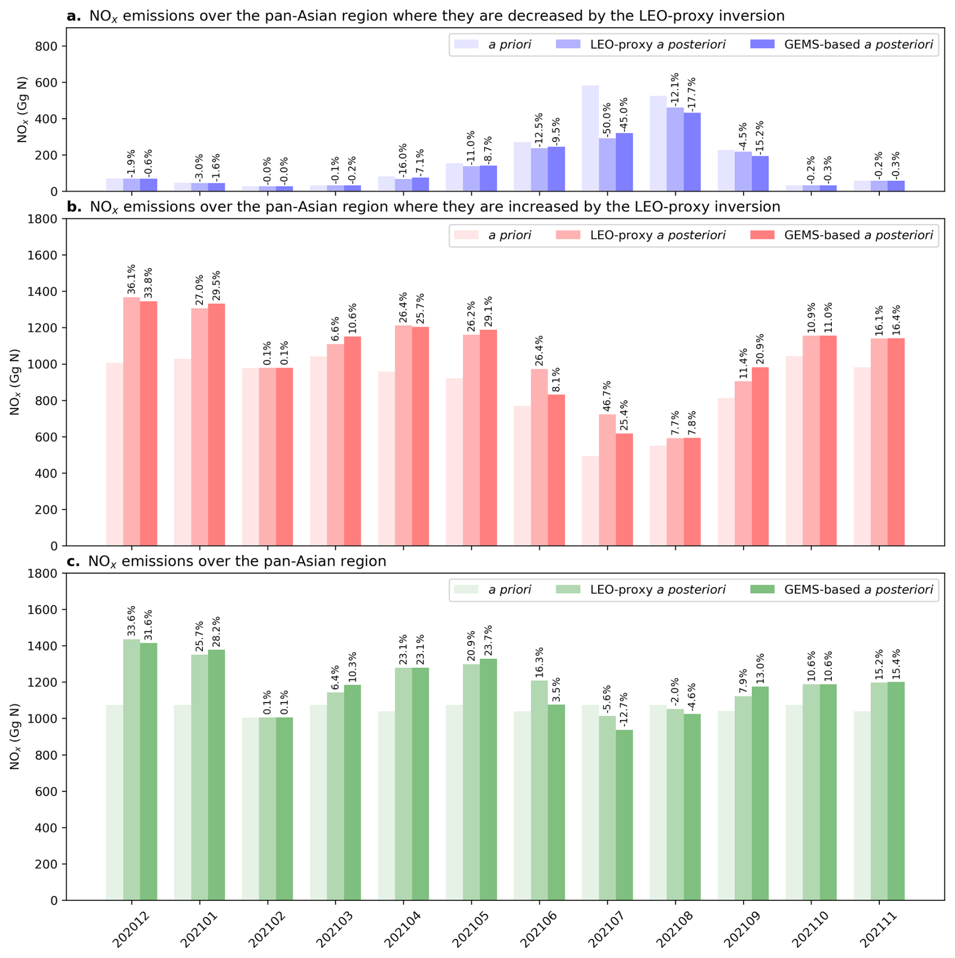
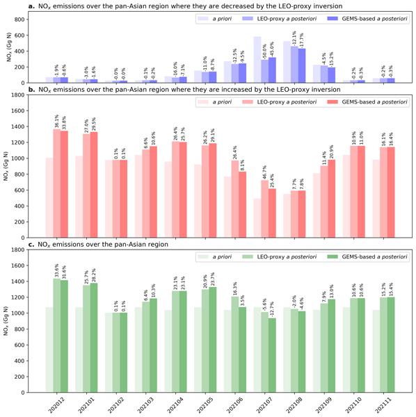
Figure 5 Anthropogenic NO_x emissions, expressed in Gg N, aggregated over the pan–Asian region (c) and their components corresponding to the areas where they are decreased (a) and increased (b) by the “LEO-proxy” inversion, respectively.

By aggregating anthropogenic NO_x emissions over the pan-Asian region and categorising the contributions from areas where the “LEO-proxy” inversion either increases or decreases emissions, Fig. 5 illustrates the monthly variations in adjustment patterns between the two experiments. In line with the summary in Table 1, both inversions yield widespread increases in anthropogenic NO_x emissions during the non-summer months across the domain. Consequently, the regionally aggregated anthropogenic NO_x emissions (Fig. 5c) are primarily driven by contributions from areas where the “LEO-proxy” inversion identified emission increases (Fig. 5b). The “GEMS-based” inversion produces higher anthropogenic NO_x emission estimates than the “LEO-proxy” inversion in March, May, and September, reflecting more uniformly robust upward adjustments across the region. Conversely, during other non-summer months, emissions from the “GEMS-based” inversion are comparable to the “LEO-proxy” results, as the former applies a mixture of stronger and weaker upward adjustments depending on the sub-region. Overall, the anthropogenic NO_x emissions aggregated over the pan-Asian region from the two inversions differ by 0.2–52.6 Gg N per month during the non-summer months, representing 0.02 %–5.06 % of the respective a priori values. Although these regional differences appear modest, they represent bulk averages over a vast and heterogeneous domain; significantly larger contrasts emerge at finer spatial scales, as previously illustrated in Figs. 4 and S17 and further explored in Sect. 3.4.

3.4 Contrasts in modelled atmospheric constituents between GEMS-based and LEO-proxy inversions

Following the analysis in Sect. 3.3, we maintain April 2021 as a representative month to illustrate the contrasts in modelled atmospheric composition resulting from the “GEMS-based” and “LEO-proxy” inversions. Because the “GEMS-based” inversion yields larger emission increases over North China Plain and smaller increases over Northern India than the “LEO-proxy” inversion, it provides an opportunity to examine how several key atmospheric constituents that are closely coupled to NO_x emissions respond to these regional differences. Specifically, we focus on NO₂, O₃, OH, CO, HCHO, SO₂, NH₃, and secondary inorganic aerosols (sulfate, nitrate, and ammonium). For several of these species, independent in situ measurements are available to facilitate a rigorous performance evaluation.

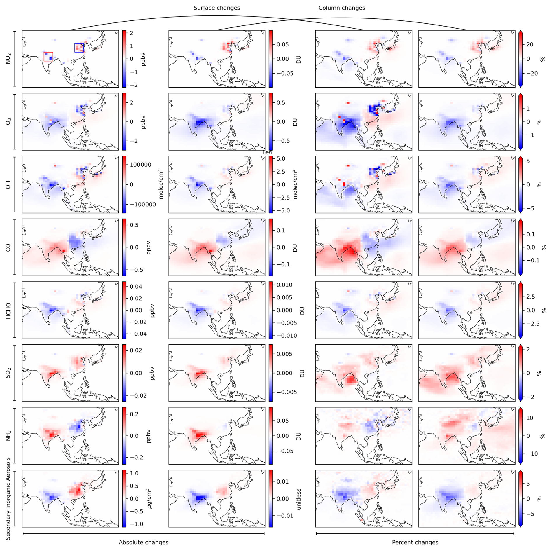
Figure 6 Absolute and percentage differences between column and surface concentrations of modelled atmospheric constituents (NO₂, O₃, OH, CO, HCHO, SO₂, NH₃, and secondary inorganic aerosols) as driven by the “LEO-proxy” and “GEMS-based” inversions in April 2021. The blue and red rectangles in the top-left panel highlight two areas where the contrasts between the two inversions are most pronounced, referred to here as the “North China Plain” and “Northern India” subregions, respectively.

Figure 6 demonstrates that the spatial hotspots of divergence in modelled constituents generally align with the spatial patterns of inferred NO_x emission differences shown in Figs. 4c1 and S17c. For instance, the “GEMS-based” inversion produces higher columnar and surface NO₂ concentrations across the North China Plain compared to the “LEO-proxy” inversion, while the inverse is observed over Northern India. Increased NO₂ can enhance HNO₃ formation and thus shift NH₃ partitioning to the particulate phase, resulting in similar patterns for secondary inorganic aerosols but an opposite pattern for NH₃. The uniform response of O₃ to different NO_x adjustments in the North China Plain and Northern India highlights the contrasting VOC-limited and NO_x-limited regimes governing O₃ production in these respective regions. Similar spatial distributions are evident for OH, which, together with O₃, determines the atmospheric oxidation capacity and consequently the removal of HCHO, CO, and SO₂. As a result, these species exhibit spatial patterns opposite to those of OH and O₃.

We acknowledge that the contrasts in modelled atmospheric constituents between the two inversions are relatively modest for most species, typically within 10 %, with surface-level changes being more pronounced than columnar adjustments. NO₂ is a notable exception, exhibiting changes of up to 20 % in both columnar and surface concentrations. This is likely because NO₂ is more directly coupled to primary NO_x emissions, whereas other species are influenced by a broader array of precursors and environmental factors. Consequently, the two inversions yield nearly identical model–observation biases for all non-NO₂ species and surface NO₂ (Fig. S18). Nonetheless, the “GEMS-based” inversion does reduce model–observation biases for AERONET columnar NO₂ measurements relative to the “LEO-proxy” for most days in April 2021 over both the North China Plain and Northern India (Fig. 7). Together with the overall model evaluation presented in Sect. 3.2, these results indicate that the “GEMS-based” inversion generally matches or exceeds the “LEO-proxy” inversion in improving model agreement with independent in situ measurements during non-summer months, when retrievals provide strong constraints owing to elevated NO₂ concentrations. We therefore anticipate that other atmospheric constituents also benefit from the high-frequency constraints of the “GEMS-based” inversion; even where these differences appear small, such changes can have significant implications for health and environmental impact assessments.

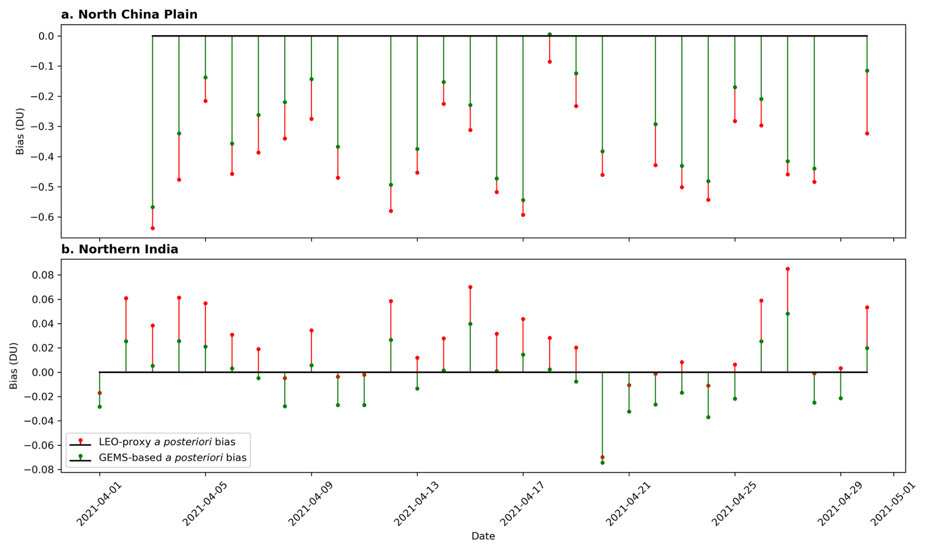
Figure 7 Stem plot of model–observation biases in column NO₂ over the North China Plain and Northern India subregions in April 2021.

To understand the added value of GEMS geostationary observations of tropospheric NO₂ for NO_x emission constraints and subsequent air quality modelling during the non-summer months, we examine the diurnal variability of the observational part of the cost function (J_obs). Figure S19 illustrates an example for April 2021. Although J_obs at 13:45 local time (KST) accounts for only a small fraction (12.1 %) of the total J_obs, it correlates well with the total J_obs, with a Pearson correlation coefficient of 0.89. This indicates that the 13:45 KST retrievals, used in the “LEO-proxy” inversion, capture a substantial portion of the information content in the full GEMS dataset. Nevertheless, the remaining 87.9 % of J_obs from other hourly retrievals also contributes to the optimization process. The degree to which these additional observations differ from the 13:45 KST retrievals, and thus provide unique information, ultimately determines the added value of the GEMS geostationary sampling.

4 Conclusions

In this study, we rigorously assess the added value of GEMS geostationary satellite observations of tropospheric NO₂ for constraining monthly NO_x emissions and subsequent air quality modelling over a full annual cycle across the pan-Asian region. We conduct this assessment by comparing two 4D-Var inversion experiments using the GEOS-Chem adjoint model: a “GEMS-based” inversion assimilating the full hourly dataset and a “LEO-proxy” inversion utilising a subset of observations at 13:45 local time (KST) as a surrogate for LEO data.

During the non-summer months (September to May), we find that both inversions yield widespread increases in NO_x emissions. Given that our a priori anthropogenic NO_x emissions are based on 2020, these increases likely reflect the rebound of anthropogenic activities in 2021 relative to the COVID-19 lockdown period in 2020, as also reported in other inversion studies (Abeed et al., 2025). The “GEMS-based” estimates vary above or below “LEO-proxy” levels depending on the month and location, with spatial contrasts mirroring the differences in retrieval density between the full and single-overpass datasets. These adjustments propagate to several modelled atmospheric constituents, including NO₂, O₃, OH, CO, HCHO, SO₂, NH₃, and secondary inorganic aerosols, where divergent responses reflecting the complex, nonlinear atmospheric chemistry and coupling between NO_x and these trace gases and aerosols. Independent evaluation against in situ columnar and surface NO₂ measurements confirms that the “GEMS-based” inversion generally matches or outperforms the “LEO-proxy” version during non-summer months, when retrievals provide strong constraints owing to elevated NO₂ conditions. Conversely, during the summer (June to August), both inversions show degraded performance relative to the a priori simulation, likely because low NO₂ conditions for which a larger fraction originates from lightning and other background sources with greater uncertainties challenge our 4D-Var framework. We acknowledge that the robustness of this seasonal contrast between the non-summer and summer months may be influenced by uncertainties in the in situ measurements used for independent evaluation. In particular, AERONET columnar NO₂ measurements may be subject to biases because they are sourced from OMI retrievals. Nonetheless, Pandora NO₂ measurements are widely regarded as a benchmark reference for ground-based NO₂ observations, with a reported clear-sky precision of approximately 0.01 DU (Herman et al., 2009), and surface NO₂ concentrations are obtained from direct measurements. The consistency of our results across multiple independent datasets lends confidence to our conclusions.

As stated in Sect. 1, only a few studies have investigated the added value of GEMS geostationary observations for top-down emission estimates (Xu et al., 2023; Park et al., 2024, 2025). We extend these efforts by providing critical insights into the benefits and technical challenges of integrating high-frequency satellite data into operational air quality management and policy-making frameworks. To ensure a controlled comparison, we optimised only monthly NO_x emissions without adjusting their empirical temporal profiles. Although this approach underuses the high-frequency information available in the “GEMS-based” dataset, we consider it necessary because the “LEO-proxy” inversion lacks the temporal resolution to adjust diurnal profiles. Nonetheless, this approach helps disentangle the benefits arising from geostationary observations themselves from those associated with advanced methodologies enabled by these observations (e.g., improved diurnal scaling factors), which have often been intertwined in previous studies (Park et al., 2024, 2025). The seasonal contrast between non-summer and summer months revealed in this study suggests two complementary directions for future research. First, the more reliable non-summer data could be used to derive hourly emissions, and the added value of such high-temporal-resolution estimates relative to conventional monthly emission estimates could then be quantified. Second, further work is needed to investigate the factors responsible for the degraded performance of GEMS data during summer and to identify strategies for improving their utility under these conditions. Both directions would benefit from adaptive error characterisation and finer-resolution modelling. The application of artificial intelligence methods to GEMS data is also encouraged for future research (He et al., 2022; Kan et al., 2024; Liu et al., 2026).