Advancing isotope-enabled model for comprehensive understanding of atmospheric sulfur isotope effects: demonstrating the overlooked isotopic fractionation during combustion and flue gas desulfurization

The isotopic composition of atmospheric species provides fundamental insights into their sources, sinks, and chemical processes. Conventional end-member mixing models, however, cannot capture progressive isotopic evolution in open systems where mixing and reaction proceed simultaneously. This limitation hinders a comprehensive understanding of the isotope effect and its atmospheric applications. Here, we develop an isotope-enabled chemical transport model (CTM) that tracks four sulfur isotopologues (³²SO₂, ³⁴SO₂, ³²SO₄²⁻, ³⁴SO₄²⁻) through emissions, transport, chemistry, and deposition. An iterative time-splitting method reduces the numerical bias from applying the Rayleigh equation in the open atmosphere. The model reproduces the ³⁴S enrichment of sulfate relative to SO₂ and captures the spatial and seasonal patterns of the sulfur isotope effect across eastern China (simulated Δδ³⁴S_SO₄²⁻ $/$ SO₂=6.11 ‰ ±1.85 ‰; observed =3.43 ‰ ±1.11 ‰). Further, the agreement between simulated (with δ³⁴S_SO₂=0 ‰ emission assumption) and observed sulfate isotopic compositions, combined with the documented higher δ³⁴S values of coal at 1 ‰–10 ‰ across eastern China, implies a systematic ³⁴S depletion in emitted SO₂ relative to fuels. This highlights the importance of considering isotopic fractionation during combustion, flue gas desulfurization and chemical processes for accurate source apportionment. The isotope-enabled model provides a new approach for constraining the sulfur budget.

1 Introduction

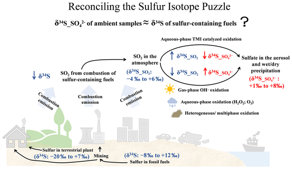
Sulfate and sulfur dioxide (SO₂) have complex interactions with the environment and Earth's climate system, involving aerosol and cloud formation, climate cooling, and the global sulfur budget (Seinfeld and Pandis, 2016). The primary sources of SO₂ emissions are from the combustion of sulfur-containing fuels (coal and oil, etc.) at power plants, industrial facilities, and residential heating (Crippa et al., 2023). The atmospheric oxidation of SO₂ to sulfate has been extensively investigated through gas-phase reactions with OH radicals and heterogeneous/multiphase oxidation involving H₂O₂, O₃, NO₂, and transition metal ion catalysis (TMI-catalysis).

Recent investigations into sulfate isotopic composition have emerged as promising proxies for gaining fundamental insight into the sulfate's sources, sinks, and concentration-independent information on atmospheric oxidation processes. However, there remains a significant discrepancy among studies that use the end-member mixing model. Han et al. (2016a) emphasized the dominance of biological sulfur emissions in summer and coal combustion in winter. Lin et al. (2022) illustrated how isotopic fractionation significantly reshapes the sulfur isotopic composition in sulfate, leading to distinctive results of source apportionment. While Feng et al. (2023) highlighted the impact of sulfur isotopic fractionation during combustion on source apportionment, identifying traffic emissions (49 %) and coal combustion (46 %–65 %) as major contributors to sulfate during heavy pollution in the North China Plain. Discrepancies also arise in identifying the dominant SO₂ oxidation pathway. Fan et al. (2020) highlighted SO₂ oxidized by NO₂ and TMI-catalyzed O₂ as a key contributor to high sulfate loading using δ³⁴S_SO₄²⁻. While Han et al. (2022) revealed enhanced SO₂ oxidation by H₂O₂, supported by δ³⁴S_SO₂ and δ³⁴S_SO₄²⁻ analyses. Several limitations may explain these divergences. (1) Studies rely on the Rayleigh distillation equation, which is only suitable for closed systems with reservoir-limited conditions, leading to an increasing apparent isotope effect as the reservoir is progressively consumed (Guan and Liu, 2023). (2) Laboratory studies have indicated that the combustion process, atmospheric chemistry and mixing can reshape the sulfur isotopic composition from the sources of sulfur-containing fuels to SO₂ and sulfate.

Therefore, our goal is to reconcile the ongoing debate among previous research findings related to sulfur isotope tracing and establish a comprehensive understanding of the atmospheric isotope effect. To achieve this, developing an isotope-enabled model that integrates isotopic chemistry and the isotopic fingerprints of emission sources is crucial. Recent applications have incorporated isotope effects into CTMs to simulate δ¹⁵N of atmospheric NO_x and NO₃⁻ using CMAQ (Fang and Michalski, 2022) and mercury isotopic fractionation using GEOS-Chem (Song et al., 2022). These methodologies involve using isotopologues as prognostic tracers and scaling the rate constants of different isotopologues with their corresponding isotope fractionation factor. However, these models primarily focus on “gas-phase” or one-step unidirectional kinetic reactions. Sulfur chemistry involves heterogeneous and multiphase reactions with mass transfer, dissociation equilibrium, and chemical reaction. Determining reaction intermediates and their isotopic fractionation factors for each elementary step is therefore challenging. In addition, the isotope effects obtained from laboratory studies for complex reactions represent apparent or overall isotope effects. Consequently, the incorporation of isotopic chemistry into CTMs faces new challenges, especially with heterogeneous/multiphase reactions.

In this study, we develop a new isotope-enabled model to simulate the isotopic compositions of sulfur-bearing species, considering both physical mixing and isotopic fractionation due to chemical reactions, and enabling the explicit simulation of progressive depletion/enrichment in the reservoir and their impact on sulfate production. The study aims to present a comprehensive description of the isotope-enabled model, evaluate its skill in reproducing the spatial-temporal variations in sulfur isotope composition, and deepen our understanding of the atmospheric sulfur isotope effects.

2 Methodology

2.1 Model framework

We incorporate the isotopic chemistry module into the Eulerian atmospheric chemistry transport models NAQPMS. The NAQPMS is a Nested Air Quality Prediction Model System developed by the Institute of Atmospheric Physics (IAP), Chinese Academy of Sciences (CAS) (Wei et al., 2019; Chen et al., 2021; Wang et al., 2001), including physical processes (advection, diffusion, and dry/wet deposition), chemistry module (gas and aqueous chemistry, aerosol chemistry and thermodynamics, and mercury chemistry) (Chen et al., 2015), and online emission of dimethyl sulfide, sea salt, and dust. The Advanced Particle Microphysics module (APM) and 1.5-D Volatility Basis Set (VBS) aerosol schemes are also coupled to simulate the aerosol microphysical processes and organic aerosol formation, respectively (Chen et al., 2019; Yang et al., 2019; Chen et al., 2014).

The simulation is performed with a two-way nested configuration. The external domain D1 covers the mainland of China at a horizontal resolution of 45 km, while the innermost domain D2 is centered over eastern China with a finer resolution of 15 km, as illustrated in Fig. 1. The model runs on 20 atmospheric vertical layers, utilizing terrain-following hybrid sigma coordinates from the surface to an altitude of 20 km. The sulfur chemistry from SO₂ to S(VI) involves gas, heterogeneous and aqueous-phase oxidation. The gas-phase chemistry incorporates the Carbon Bond Mechanism Z (CBM-Z) (Zaveri and Peters, 1999). For aqueous chemistry, the Regional Acid Deposition Model (RADM2) is applied, resolving cloud-phase sulfur oxidation through dissoluble S(IV) with O₃, H₂O₂, proxy acetic acid (CH₃OOH), and transition metal-catalyzed O₂ (Stockwell et al., 1997). The oxidation of S(IV) species by dissolved NO₂ is also incorporated into the sulfur aqueous chemistry, referring to the kinetic parameters proposed by Cheng et al. (2016). Heterogeneous reactions of SO₂ on various surfaces, including dust, sea salt, soot and deliquesced aerosols, have also been incorporated using the reactive uptake coefficients parameterization (Li et al., 2018). The gas-particle partitioning of inorganic aerosols and aerosol water content are simulated using the improved ISORROPIA II (Fountoukis and Nenes, 2007; Song et al., 2018). The simulation began in March 2014. The initial 3 months served as a spin-up time. For additional details on the model and its detailed configuration, refer to Sect. S1 and Table S2 in the Supplement.

Figure 1 Model domain and compiled sulfur isotopic composition (δ³⁴S) data. The simulation uses a two-way nested configuration, with the parent domain D1 covering the Chinese mainland (45 km resolution) and the child domain D2 centered over eastern China (15 km resolution). Literature-reported δ³⁴S data are overlaid at sampling locations. Black, red, and green bars denote the mean ±1 standard deviation of δ³⁴S of coal, aerosol sulfate, and wet precipitation sulfate, respectively. The small black bar near Inner Mongolia denotes coal δ³⁴S value only (regional mean =0.8 ‰), no aerosol or wet precipitation sulfate δ³⁴S are available there. All values are in per mil (‰). Additional details on the observed data can be found in Table S1.

2.2 Isotope notation and isotopic fractionation

The sulfur element is widely present throughout all natural environments and possesses four stable isotopes, namely ³²S, ³³S, ³⁴S, and ³⁶S, with relative abundances of 95.02 %, 0.75 %, 4.21 %, and 0.02 %, respectively (De Laeter et al., 2003). In general, the sulfur isotopic composition is denoted as δ^xS value in per mil (‰), where ^xS represents one of the less abundant isotopes, e.g., ³³S, ³⁴S, or ³⁶S. This notation is defined as the difference between the isotopic ratio of a given sample and the reference standard V-CDT (Vienna Canyon Diablo Troilite):

$$\begin{array}{}\text{(1)}& {\mathit{\delta }}^x{\mathrm{S}}_{\mathrm{Sample}}\left(\mathrm{‰}\right)=\left({\displaystyle \frac{R{(}^x\mathrm{S}{/}^{\mathrm{32}}\mathrm{S}{)}_{\mathrm{Sample}}}{R{(}^x\mathrm{S}{/}^{\mathrm{32}}\mathrm{S}{)}_{\text{V-CDT}}}}-\mathrm{1}\right)\times \mathrm{1000}\end{array}$$

where R represents the isotopic ratio, defined as the atomic abundance ratio of heavier to lighter stable isotope, expressed as $R=N{(}^{\mathrm{h}}X)/N{(}^{\mathrm{l}}X)$, where N(^hX) and N(^lX) represent the atomic abundances of the heavier stable isotope (^hX) and lighter stable isotope (^lX), respectively. V-CDT is the international sulfur isotope standard, with isotopic ratios of R(³⁴S/³²S)_V-CDT=0.044163 and R(³³S/³²S)_V-CDT=0.007877 (Ding et al., 2001).

Isotope effects are observable in physical or chemical processes, especially during equilibrium (or thermodynamic) and kinetic processes, leading to a change in isotope distribution between two substances or different phases of the same substance with distinct isotope ratios. Isotopic fractionation is often a result of the isotope effect. The isotopic fractionation factor α ${}^{\mathrm{h}}{X}_{\mathrm{P}/\mathrm{S}}$ is defined as the ratio of isotopic ratio of the instantaneously formed product $R_{\mathrm{Pi}}=\left(N{(}^{\mathrm{h}}X\right)/N{(}^{\mathrm{l}}X){)}_{\mathrm{Pi}}$ and substrate $R_{\mathrm{S}}=\left(N{(}^{\mathrm{h}}X\right)/N{(}^{\mathrm{l}}X){)}_{\mathrm{S}}$ (Mariotti et al., 1981),

$$\begin{array}{}\text{(2)}& \mathit{\alpha }{}^{\mathrm{h}}{X}_{\mathrm{P}/\mathrm{S}}=R_{\mathrm{Pi}}/R_{\mathrm{S}}\end{array}$$

For thermodynamic (equilibrium) or unidirectional kinetic process with a single-step reaction following a first-order rate law, the $\mathit{\alpha }{}^{\mathrm{h}}{X}_{\mathrm{P}/\mathrm{S}}$ can be interpreted as the ratio of rate constant k or equilibrium constant K:

$$\begin{array}{}\text{(3)}& \mathit{\alpha }{}^{\mathrm{h}}{X}_{\mathrm{P}/\mathrm{S}}={}^{\mathrm{h}}k{/}^{\mathrm{l}}k={}^{\mathrm{h}}K{/}^{\mathrm{l}}K\end{array}$$

An isotope enrichment factor, ϵ (in per mil ‰), can be defined as:

$$\begin{array}{}\text{(4)}& \mathit{ϵ}=(\mathit{\alpha }{}^{\mathrm{h}}{X}_{\mathrm{P}/\mathrm{S}}-\mathrm{1}){}^{*}\mathrm{1000}\end{array}$$

The $\mathit{\alpha }{}^{\mathrm{h}}{X}_{\mathrm{P}/\mathrm{S}}$ determines how much faster or slower the reaction with the heavier isotopologues proceeds relative to the reaction with the lighter isotopologues.

Generally, isotopic fractionation determined in laboratory experiments represents overall isotope effects, resulting from physical, equilibrium, and kinetic fractionation. The isotopic composition between reservoir and product, as a function of reactant extent and fractionation factor, is described by the Rayleigh fractionation equation.

$$\begin{array}{}\text{(5)}& R_{\mathrm{S},t}/R_{\mathrm{S},t\mathrm{0}}={f_{\mathrm{rem}}}^{({\mathit{\alpha }}^{{}^{\mathrm{h}}{X}_{\mathrm{P}/\mathrm{S}}}-\mathrm{1})}\end{array}$$

where f_rem is the fraction of residual reactant, R_S,t0 and R_S,t are the isotope ratio of substrate at initial t₀ and t moment, respectively. The instantaneous isotope ratio of the product R_P,t at t moment is given by:

$$\begin{array}{}\text{(6)}& R_{\mathrm{P},t}/R_{\mathrm{S},t\mathrm{0}}={\mathit{\alpha }}^{{}^{\mathrm{h}}{X}_{\mathrm{P}/\mathrm{S}}}\times {f_{\mathrm{rem}}}^{({\mathit{\alpha }}^{{}^{\mathrm{h}}{X}_{\mathrm{P}/\mathrm{S}}}-\mathrm{1})}\end{array}$$

The average isotope ratio of accumulated product ($\stackrel{\mathrm{‾}}{R_{\mathrm{P}}}$) during a finite reaction interval follows the standard Rayleigh-fractionation expression for accumulated products (Hoefs, 2018):

$$\begin{array}{}\text{(7)}& \stackrel{\mathrm{‾}}{R_{\mathrm{P}}}/R_{\mathrm{S},t\mathrm{0}}={\displaystyle \frac{\mathrm{1}-{f_{\mathrm{rem}}}^{({\mathit{\alpha }}^{{}^{\mathrm{h}}{X}_{\mathrm{P}/\mathrm{S}}}-\mathrm{1})}}{\mathrm{1}-f_{\mathrm{rem}}}}\end{array}$$

2.3 Developing Isotope-Tagged Emission Inventories

The multi-resolution Emission Inventory for China (MEIC, http://meicmodel.org.cn/?p=1579&lang=en, last access: 11 August 2026) provides a comprehensive SO₂ emission inventory, including anthropogenic emissions from power plants, industry, residential, and transportation, respectively. Primary combustion sulfate, which forms as the oxidation product in the chimney and plumes (Sun et al., 2023; Ding et al., 2021), is assumed to be 5 wt % of anthropogenic SO₂ (Berglen et al., 2004). Anthropogenic sulfur-containing sources exhibit a highly variable and overlapping isotopic composition, ranging from −30 ‰ to 30 ‰ (Hoefs and Harmon, 2022). We adopt a constant signature of δ³⁴S =0 ‰ V-CDT for anthropogenic SO₂ emission sources. This simplification isolates the atmospheric chemical isotope effect from poorly constrained source signatures.

The sulfur isotope difference between SO₂ and sulfate (Δδ³⁴S_SO₄²⁻ $/$ SO₂=δ³⁴S_SO₄²⁻–δ³⁴S_SO₂) approximates the apparent isotopic fractionation multiplied by 1000 ‰ and is hereafter referred to as the isotope effect. Δδ³⁴S_SO₄²⁻ $/$ SO₂ is mathematically independent of the absolute emission δ³⁴S and can be therefore validate the oxidation module of isotope-enabled CTM. By contrast, the δ³⁴S_SO₂ and δ³⁴S_SO₄²⁻ depend on the prescribed emission signature. Direct comparisons between simulated and observed δ³⁴S_SO₂ and δ³⁴S_SO₄²⁻ are subject to the uncertainties of this assumption and should be interpreted with caution. Jointly examining the simulated and observed δ³⁴S_SO₂ and δ³⁴S_SO₄²⁻ together with Δδ³⁴S_SO₄²⁻ $/$ SO₂ provides a diagnostic of whether a given model–observation bias arises primarily from the atmospheric oxidation processes or from the assumed emission-source signatures.

The tracer mass of ³²SO₂, ³⁴SO₂, ³²SO₄²⁻, ³⁴SO₄²⁻ isotopologues can be determined from the SO₂ mass in the emission inventory based on the Eq. (1), with the initial values of R_V-CDT at 0.044163.

$$\begin{array}{}\text{(8)}& {}^{\mathrm{34}}\mathrm{S}={}^{\mathrm{32}}\mathrm{S}\times \left(({\displaystyle \frac{{\mathit{\delta }}^{\mathrm{34}}\mathrm{S}}{\mathrm{1000}}}+\mathrm{1})\times R_{\text{V-CDT}}\right)\end{array}$$

2.4 Coupled methodology of isotopic chemistry module

2.4.1 The development of isotopic chemistry module

To dynamically simulate the spatiotemporal distribution of isotopic composition (δ³⁴S) in particle SO₄²⁻ and its gaseous precursor SO₂, we have implemented the tagging technology and isotopic chemistry module into the atmospheric chemistry transport model. The four isotopologues (³²SO₂, ³⁴SO₂, ³²SO₄²⁻, ³⁴SO₄²⁻) are treated as independent prognostic tracers of SO₂ and sulfate aerosol throughout their entire atmospheric life cycle, including emission, transport, chemical production/loss, and deposition processes.

Generally, previous isotope-enabled models incorporating isotope chemistry typically only consider kinetic isotope fractionation, deriving different rate coefficients for individual isotopologues from isotopic fractionation factors (α) with Eq. (4) (Fang and Michalski, 2022; Gromov et al., 2010). This assumption is suitable for single-step, steady-state reactions, such as gas-phase chemical reactions. However, most processes in natural systems involve reaction sequences; each reaction within the sequence exhibits its intrinsic isotope fractionation, and not all isotope fractionation of these individual reactions is measurable. For example, the cloud and aqueous-phase chemical module involve gas-to-particle equilibrium, dissolution, diffusion, and chemical reactions. Thus, the isotope effect observed in the complex system with multiple intermediates represents an overall isotope effect. If the reaction sequences have a given end product, the conventional approach for deriving the isotope effect requires repeated determination of R_S,t0, $\stackrel{\mathrm{‾}}{R_{\mathrm{P}}}$ and f_rem. The isotope fractionation factor is then calculated using the Rayleigh equation as,

$$\begin{array}{}\text{(9)}& \stackrel{\mathrm{‾}}{R_{\mathrm{P}}}=R_{\mathrm{S},t\mathrm{0}}\times {\displaystyle \frac{\mathrm{1}-{f_{\mathrm{rem}}}^{({\mathit{\alpha }}^{{}^{\mathrm{h}}{X}_{\mathrm{P}/\mathrm{S}}}-\mathrm{1})}}{\mathrm{1}-f_{\mathrm{rem}}}}\end{array}$$

When a substrate is consumed through multiple competing pathways simultaneously, the Rayleigh equation relates the change in the isotopic ratio of substrate to the extent of substrate consumption, employing the apparent overall isotopic fractionation factor (α_A) (Van Breukelen, 2007). The factor of α_A is expressed as a function of various instantaneous isotopic fractionation factors (α_ins) associated with individual pathways, given by the following equation:

$$\begin{array}{}\text{(10)}& {\mathit{\alpha }}_{\mathrm{A}}=F_{\mathrm{1}}\times {\mathit{\alpha }}_{\mathrm{ins}\mathrm{\_}\mathrm{1}}+F_{\mathrm{2}}\times {\mathit{\alpha }}_{\mathrm{ins}\mathrm{\_}\mathrm{2}}+\mathrm{\dots }+F_n\times {\mathit{\alpha }}_{\mathrm{ins}\mathit{\_}n}\end{array}$$

Therefore, the sulfur isotopic ratio of the residual SO₂ within the grid cell can be determined using the following equation:

$$\begin{array}{}\text{(11)}& R_{\mathrm{S},t}=R_{\mathrm{S},t\mathrm{0}}\times {f_{\mathrm{rem}}}^{({\mathit{\alpha }}_{\mathrm{A}}-\mathrm{1})}=R_{\mathrm{S},t\mathrm{0}}\times {f_{\mathrm{rem}}}^{(\sum F_i\times {\mathit{\alpha }}_{\mathrm{ins}\mathit{\_}i}-\mathrm{1})}\end{array}$$

here F_i is the ratio of contribution from the ith process to the overall product.

To directly apply isotope fractionation factors measured in laboratory studies, we developed an independent isotopic chemistry module coupled to the host CTM, as illustrated in Fig. 2. The module utilizes Rayleigh-fractionation equations to calculate isotopologues changes between reactants and products, combined with the iterative time-splitting method described in Sect. 2.4.2 to reduce numerical bias. At each model time step, the module receives SO₂ loss and sulfate production separately from the gas-phase, heterogeneous, and cloud/aqueous-phase chemistry modules, and the relative contribution of each oxidation pathway is calculated and recorded. Temperature-dependent isotope fractionation factors are then updated in each grid cell according to the local temperature. The module tracks the net changes in four isotopologues (³²SO₂, ³⁴SO₂, ³²SO₄²⁻, ³⁴SO₄²⁻) and updates their concentrations through an iterative time-splitting procedure, which divides each oxidation calculation into smaller SO₂ conversion sub-steps. Within each sub-step, isotope ratios are calculated using Rayleigh-fractionation equations, isotopic mass balance is enforced, and the isotopic composition of the reactant reservoir and accumulated product is updated. The full algorithm framework is further documented in Sect. S2.

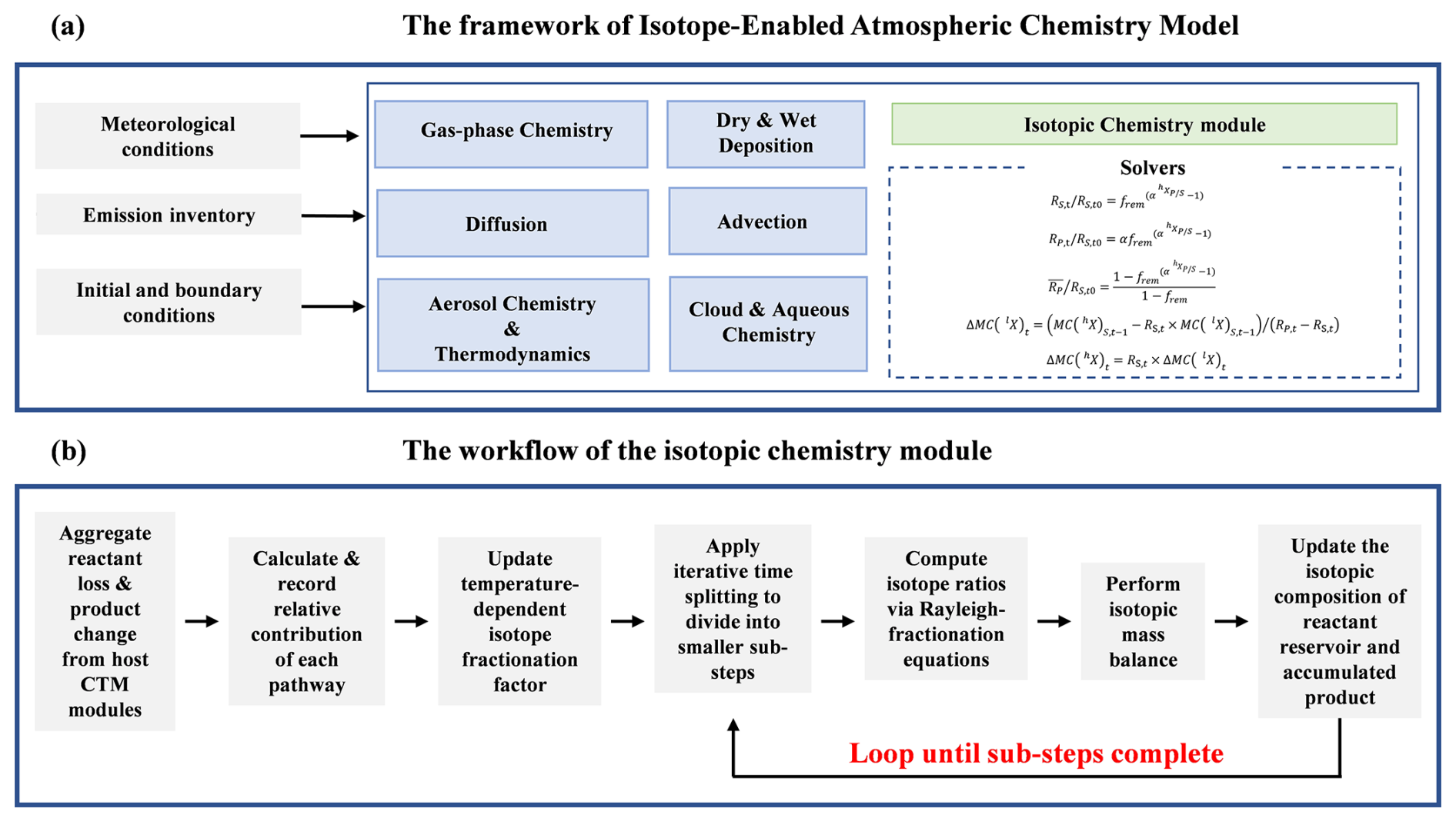
Figure 2 Algorithmic framework of the isotope-enabled CTM and the isotopic chemistry module. (a) Host CTM framework, including the main physical and chemical modules (gas-phase chemistry, aerosol chemistry and thermodynamics, cloud and aqueous chemistry, advection, diffusion, and dry and wet deposition) and their coupling with the isotopic chemistry module. (b) The workflow of the isotopic chemistry module. At each time step, the module tracks net SO₂ and sulfate changes, calculates reaction fractions, updates temperature-dependent fractionation factors, applies iterative time splitting, computes isotope ratios via Rayleigh-fractionation equations, performs isotopic mass balance, and updates the isotope ratios of the reactant reservoir and accumulated product.

Based on the assumptions outlined in Sect. S1, the δ³⁴S is primarily influenced by fractionation during different chemical reactions. Relevant sulfur isotopic fractionation data have been sourced from laboratory studies conducted by Harris et al. (2012b, 2012a, 2012c, 2013), including the gas-phase oxidation by OH radicals, aqueous-phase oxidation by H₂O₂, O₃, and iron catalysis, heterogeneous oxidation of SO₂ on sea salt aerosol and mineral dust (see Table 1). The sulfur isotopic fractionation during SO₂ oxidation by NO₂ in the aqueous phase, as determined by Yang et al. (2018), is excluded from this study. This exclusion is attributed to their methodology, which yielded an apparent isotopic fractionation factor calculated by dividing the isotopic ratio of accumulated production by the initial isotope ratio of reactant. This calculation assumed that R_pi was approximated by $\stackrel{\mathrm{‾}}{R_{\mathrm{P}}}$ with f_rem being approximately 1. This approach contrasts with the conventional definition of the isotope fractionation factor, which typically represents the isotope ratio in the instantaneously formed product in an infinitely short time divided by that of the reactant (Eq. 2) (Harris et al., 2013; Hoefs, 2018; Mariotti et al., 1981). For reference in our discussion, the apparent isotopic fractionation factor α³⁴S${}_{{\mathrm{NO}}_{\mathrm{2}}}$ (T at 3 °C) =0.998 is adopted in the simulation.

Table 1 The sulfur isotopic fractionation factor determined by the lab experiment and its temperature dependency for a specific oxidation pathway.

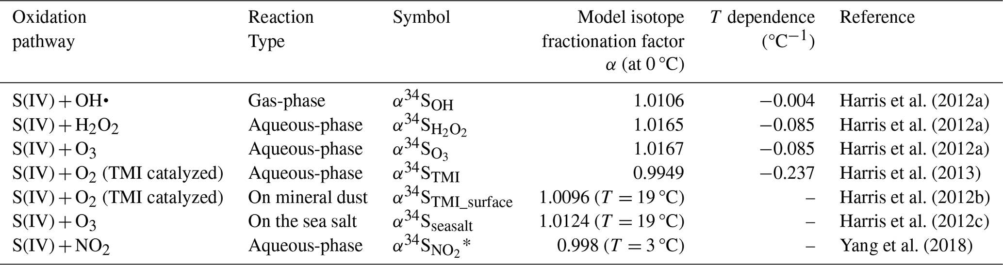
We consider the temperature dependence of the isotopic fractionation factor by utilizing the real-time temperature of the grid cell, thus avoiding a significant effect on the seasonal simulation of isotopic composition. α³⁴S${}_{{\mathrm{NO}}_{\mathrm{2}}}{}^{*}$ denotes the apparent isotopic fractionation factor during SO₂ oxidation by NO₂ in the aqueous phase at 3 °C, α³⁴S${}_{{\mathrm{NO}}_{\mathrm{2}}}$ (T at 3 °C) $=\mathrm{0.998}\pm \mathrm{0.00041}$, was determined by Yang et al. (2018). In their laboratory experiment, SO₂ was oxidized by NO₂ in a reaction chamber containing liquid water. The isotopic composition δ³⁴S in the initial SO₂ and accumulated sulfate product after 2 h of reaction time was collected and measured. However, the residual fraction of SO₂ was not measured, and the apparent isotopic fractionation factor was calculated by dividing the isotopic ratio of accumulated production by the ratio of reactant. As the reaction progresses, the isotopic composition of the accumulated product changes. Once the reactants are completely consumed, the isotopic composition of the accumulated product is equal to the initial reactants (See Fig. 3). Therefore, according to the isotope mass balance, the apparent isotopic fractionation factor is highly dependent on the residual fraction during the reaction process, and cannot be equal to the exact isotopic fractionation factor, which is represented by the isotope ratio in the instantaneously formed product divided by the ratio in the reactant. Although the detected apparent isotopic fractionation factor can indicate the direction of isotopic fractionation (enrichment or depletion in the product relative to the reactant), it cannot be directly used in the model to calculate the isotope effect of S(IV) + NO₂ pathway.

Figure 3 Rayleigh plot for sulfur isotope fractionations during SO₂ oxidation in a closed system with no external input and irreversible product removal. δ³⁴S values of the residual reactant (solid black line), instantaneous product (blue dotted line), and accumulated product (blue dashed line) are shown as a function of the fraction of remaining reactant based on a Rayleigh equation, with the initial δ³⁴S of SO₂ set to 0 ‰. Three scenarios are illustrated: (a) aqueous-phase H₂O₂ oxidation (α³⁴S =1.0165 at 0 °C), (b) aqueous-phase TMI-catalyzed oxidation (α³⁴S =0.9949 at 0 °C), and (c) the net isotope effect under competing S(IV) oxidation pathways (α³⁴S =1.0063 at 0 °C). The pathway contributions in panel (c) competing S(IV) oxidation pathways – gas-phase OH oxidation (42.6 %), aqueous H₂O₂ oxidation (2.2 %), O₃ oxidation (1.3 %), TMI-catalyzed oxidation (27.2 %), and heterogeneous reactions (26.7 %) – are derived from GEOS-Chem simulations (Shao et al., 2019).

2.4.2 Improving isotopic chemistry simulation with the iterative time-splitting method

In CTM, numerical integration is crucial for solving the kinetic equations of chemical mechanisms. In the gas-phase module, the CBMZ mechanism is coupled with the LSODES solver (the sparse version of the Livermore ODE solver) to integrate the chemical transformations and provide species concentration changes over time. In the cloud and aqueous chemistry module, the gas–aqueous partitioning is determined by instantaneous Henry's law equilibrium; at each step, a bisection method estimates pH and ionic speciation under electroneutrality and thermodynamic equilibrium, and a forward Euler solver integrates the aqueous-phase sulfur oxidation reactions, with chemical equilibrium reestablished after each incremental oxidation step.

The classical Rayleigh distillation equation assumes that (i) the product, once formed, is immediately and irreversibly removed with no further isotopic exchange, and (ii) the reservoir receives no external input, the reactants being consumed solely by the fractionating reaction. These assumptions do not hold in the open atmosphere. Within a single integration step (∼30 min), the reactant reservoir in each grid cell is continuously influenced by emissions, advection, and diffusive mixing. Because mixing and fractionation occur simultaneously, applying the Rayleigh equation over the full-time step, especially under a large conversion fraction, makes the isotopic composition sensitive to the residual fraction f_rem, which itself depends on time discretization and reaction-rate constants. This artificially amplifies the apparent enrichment or depletion in the residual reactant, producing the so-called reservoir effect. Mitigating this bias provides the numerical motivation for the iterative time-splitting method used here.

To reduce the numerical bias that can arise when the Rayleigh equation is applied directly over a finite CTM time step in an open atmospheric system, we introduce an iterative time-splitting method that divides each oxidation calculation into smaller conversion sub-steps and updates the isotopic composition iteratively. Within each main time step, the total reactant supplied by emissions, advection, and mixing is apportioned across the sub-steps. At the start of each sub-step, the reactant concentration and isotope ratio are updated by incorporating the freshly allocated reactant, after which the Rayleigh equation is applied under the approximately closed conditions of that sub-step, where the conversion fraction is kept below 2 %. This ensures that isotope fractionation is computed incrementally in the presence of continuous fresh input, rather than over the full model time step. In addition, we derive an exact integration solution describing the isotopic evolution of the reservoir in an open system with simultaneous fresh input and product removal (Sect. S3). By comparing the iterative method against this exact benchmark, we determine the optimal sub-step size that minimizes the discrepancy between the Rayleigh-based calculation and the open-system solution; further sensitivity tests are presented in Sect. 3.1.

3 Results

Building upon the isotope-enabled modeling framework established in Sect. 2, we evaluate the model's performance. The evaluation proceeds in two stages. First, we validate the iterative time-splitting method incorporated into the isotopic chemistry calculation (Sect. 3.1), demonstrating that our approach adequately resolves the isotope evolution in open systems with simultaneous mixing and reaction. Second, we assess the model's ability to capture observed sulfur isotope signatures, focusing on the sulfur isotope effect (Δδ³⁴S_SO₄²⁻ $/$ SO₂) and the site- and season-dependent δ³⁴S_SO₄²⁻ across eastern China (Sect. 3.2).

3.1 Improving isotopic chemistry simulation and sensitivity tests

In previous studies, the initial isotopic composition of reactant (δ_s,0) was calculated based on the isotopic composition of the product (δ_p) and the residual fraction of reactants f_rem using the Rayleigh equation, assuming no addition or mixing. This resulted in isotopic “reservoir effects” as the reaction progressed. The isotopic fractionation factor determines the direction of fractionation: when α>1, heavy isotopes are preferentially enriched in the product and depleted in the residual reservoir; conversely, when α<1, heavy isotopes are preferentially depleted in the product and enriched in the residual reservoir.

To illustrate the magnitude of the reservoir effect under realistic atmospheric conditions, we consider the competing S(IV) oxidation pathways: gas-phase OH radicals, aqueous-phase H₂O₂, O₃, and TMI-catalysis, and heterogeneous reaction. Using model results from Shao et al. (2019), who employed the GEOS-Chem model to quantify the contributions of these competing pathways to sulfate formation during a Beijing pollution episode, their reported contributions are 42.6 %, 2.2 %, 1.3 %, 27.2 %, and 26.7 %, respectively. Based on these pathway contributions, the calculated overall/net sulfur fractionation factor α³⁴S_S(IV) is 1.0063 at 0 °C. Therefore, the sulfate product favors the heavier isotopologues ³⁴SO₄²⁻ over ³²SO₄²⁻, leading to an increase in δ³⁴S_SO₄²⁻ as the reaction progresses. This relationship depends on the fractionation fraction and the reaction extent. As shown in Fig. 3, with the initial δ³⁴S of SO₂ set to 0 ‰, when f_rem drops to 70 % and 20 %, the δ³⁴S of the residual SO₂ reaches approximately −2.2 ‰ and −10 ‰, while the δ³⁴S of the accumulated sulfate product reaches approximately 5.2 ‰ and 2.5 ‰, respectively. The resulting Δδ³⁴S_SO₄²⁻ $/$ SO₂ is 7.4 ‰ and 12.5 ‰. As the reservoir approaches depletion (f_rem≈0), the apparent isotope fractionation becomes unrealistically large. This challenges the direct application of the Rayleigh equation to systems where mixing and reaction occur simultaneously.

Using the integration method that describes the isotopic evolution of the reservoir in an open system (Sect. S3), Fig. S1 illustrates that as the β value (the ratio of the instantaneous amount added to the removal) increases, the δ value of the reservoir progressively gets higher, with the external sources consistently contributing with a constant isotopic composition (δ_s) of 10 ‰. This emphasizes the importance of considering the mixing process when calculating the isotope effect. The overall apparent isotope fractionations are indeed the result of combined effects of the Rayleigh-like distillation process and the diffusion-driven isotope distributions (Guan and Liu, 2023). The combined processes with the mixing of fresh material and isotopic fractionation can lead to a smaller variation in Δδ³⁴S_SO₄²⁻ $/$ SO₂ than estimated by Rayleigh equation. These results indicate that the optimal sub-timesteps effectively reduce the time-step impact and minimize discrepancies between the Rayleigh-based calculation and the integration method.

To mitigate the numerical bias that can arise when the Rayleigh equation is applied directly over a finite CTM time step, we implement an iterative time-splitting method. Firstly, the comparison between this iterative method and integration method in the open system helps determine the optimal sub-timesteps, effectively minimizing the biases in isotopic calculation when employing the Rayleigh equation. Figure S2 illustrates that the largest differences are observed for small reaction fraction and large fraction of fresh mixture relative to the initial substrate. A larger difference is expected when the differences between the isotopic composition of substrate and mixture increase and the isotope effect becomes stronger. For 50 sub-timesteps, good agreements are found in the calculated isotopic value of the reservoir between the iterative time-splitting method and the integrating method, assuming 0.3 ‰ is approximate to the average analytical precision of isotope. This indicates that the combination of the Rayleigh equation with the iterative method is capable of effectively simulating the progressive isotopic evolution of reservoirs with simultaneous mixing and isotopic fractionation.

We also conduct sensitivity tests to check the performance of the simulated isotopic composition of product with the optimized sub-timesteps. We choose 0.3 ‰ as the tolerance of this iterative time-splitting method. Figure S3 illustrates the deviation of δ-values for 1, 10, 50, and 100 sub-steps relative to the reference simulation with 1000 sub-steps. Notably, the largest deviation occurs for a large fraction of reaction f and mixture, attributed to greater depletion in the reservoirs (α>1) and influence of mixing process. For 50 sub-steps, the maximum deviation is less than 0.1 ‰. This comparison confirms that the sub-timestep limiting reaction fraction f to approximately 2 % is acceptable for reducing simulation bias, thus the value is adopted to improve the simulation.

The numerical comparison further shows that the largest differences between the direct Rayleigh calculation and the iterative method occur mainly over remote oceanic regions, where SO₂ emissions are low, reaction extents are high, and the SO₂ reservoir effect is strongest; in these regions, the iterative method reduces the simulated Δδ³⁴S_SO₄²⁻ $/$ SO₂ by approximately 1.5 ‰–3.0 ‰ relative to the direct Rayleigh calculation applied over the full model time step. In regions with intensive anthropogenic activity, the influence is smaller but still non-negligible, with changes of approximately 0.3 ‰–1.0 ‰ in some polluted areas, demonstrating that the iterative time-splitting method improves the numerical accuracy of simulated sulfur isotope fractionation.

3.2 Model evaluation

3.2.1 Evaluation of sulfur isotope effect

As shown in Table 1, the sulfur isotopes exhibit distinctive fractionation during chemical reactions, including gas-phase, aqueous-phase, and heterogeneous reactions. It provides valuable information for investigating the relative importance of the different oxidation pathways converting SO₂ to sulfate. Gas-phase and aqueous-phase oxidation by H₂O₂ and O₃ produces sulfate that is enriched in ³⁴S (+15.1 ‰ to +19.9 ‰, depending on pH and temperature) relative to the initial SO₂ reservoir, while the SO₂ reservoir becomes depleted in ³⁴S. In contrast, TMI-catalyzed oxidation produces sulfate depleted in ³⁴S ($-\mathrm{9.5}\pm \mathrm{3.1}$ ‰) relative to initial SO₂ (Harris et al., 2012c, 2012a, 2013, 2012b).

Figures 4 and 5 show the simulated spatial-temporal distribution of near-surface δ³⁴S_SO₂ and δ³⁴S_SO₄²⁻ for individual sulfur oxidation pathways through controlled experiments. We focus on the simulation results for the isotope effect resulting from individual sulfur oxidation pathways. The δ³⁴S of all emission sources is assumed to be 0 ‰. The model predicts a daily-mean range of δ³⁴S_SO₄²⁻ of 8 ‰, 2 ‰ ∼16 ‰, 0 ‰ ∼6 ‰, and −8 ‰ ∼0 ‰ via gas-phase oxidation by OH radical, and cloud-phase oxidation by H₂O₂, O₃, TMI-catalyzed O₂ over eastern China, respectively. Correspondingly, a depleted ³⁴S in SO₂, and the daily-mean range of δ³⁴S_SO${}_{\mathrm{2}}=-\mathrm{5}$ ‰ ∼1 ‰, −5 ‰ ∼0 ‰, −3 ‰ $\sim -\mathrm{1}$ ‰, and 0.5 ‰ ∼3 ‰, respectively. A relatively homogeneous spatial pattern of δ³⁴S_SO₄²⁻ is observed for gas-phase oxidation (∼8 ‰), whereas aqueous-phase oxidations show more heterogeneous spatial distributions. The simulated spatial-temporal distribution of δ³⁴S_SO₄²⁻ depends on the relative importance of different oxidation pathways and the ratio of mixed SO₂ to formed sulfate within each model time step. Unlike gas-phase reactions, cloud and aqueous phase chemistry highly depend on the geographical distribution of cloud coverage and liquid water content. The spatial distribution of simulated δ³⁴S_SO₂ is more sensitive to the mixing rate of SO₂; in eastern China, where SO₂ emission intensity is high, the reservoir effect is effectively offset, resulting in slight regional differences.

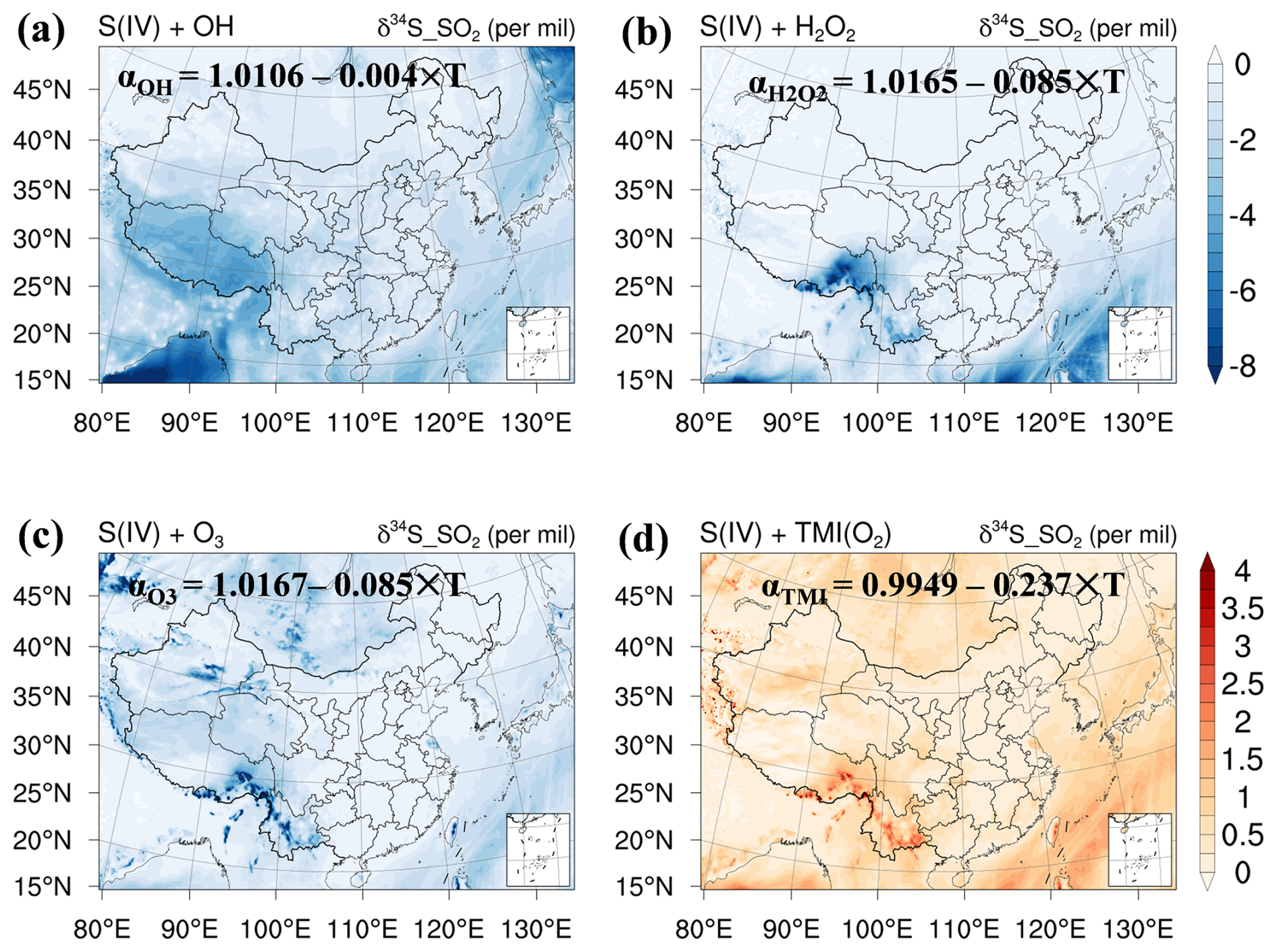
Figure 4 Simulated spatial distribution of near-surface δ³⁴S_SO₂ for individual sulfur oxidation pathways. Each panel shows the result of a sensitivity experiment in which only one oxidation pathway is active: (a) gas-phase oxidation by OH radical, (b) cloud-phase oxidation by H₂O₂, (c) cloud-phase oxidation by O₃, and (d) cloud-phase oxidation by TMI-catalyzed O₂. All simulations are for December 2015. The sulfur isotopic composition of all emission sources is set to 0 ‰ to minimize the impact of source fingerprint, reflecting the direction and magnitude of the isotope fractionation specific to each pathway. Positive values indicate ³⁴S enrichment in residual SO₂; negative values indicate depletion.

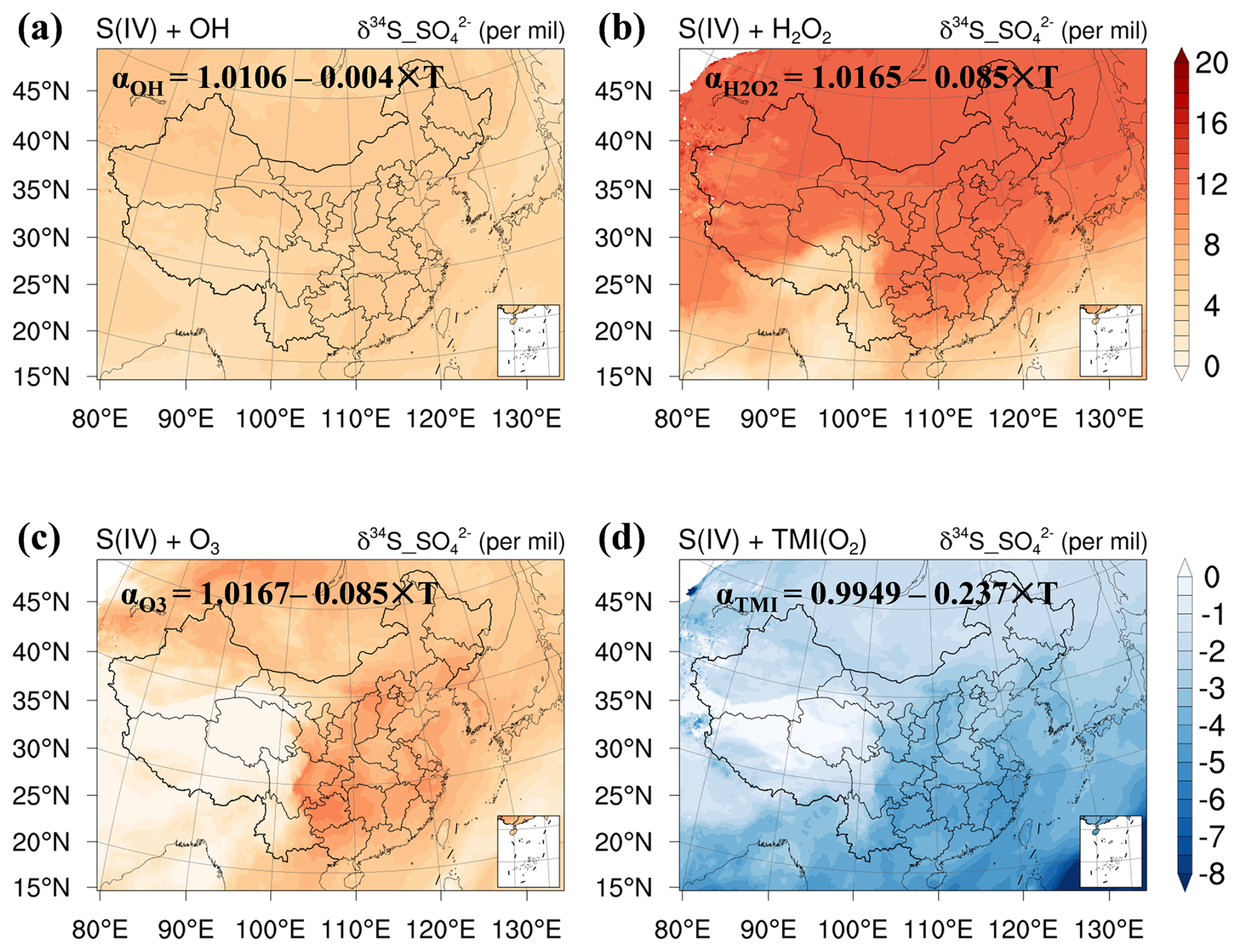
Figure 5 Same as Fig. 4, but for near-surface δ³⁴S_SO₄²⁻. Panels show sensitivity experiments with individual oxidation pathways active: (a) gas-phase OH, (b) aqueous-phase H₂O₂, (c) aqueous-phase O₃, and (d) TMI-catalyzed O₂ oxidation, all for December 2015 with δ³⁴S_SO₂ emission =0 ‰. Positive values indicate ³⁴S enrichment in sulfate; negative values indicate depletion.

We evaluate the oxidation isotope module using the sulfur isotope effect Δδ³⁴S_SO₄²⁻ $/$ SO₂, the isotopic difference between sulfate and SO₂. Because Δδ³⁴S_SO₄²⁻ $/$ SO₂ depends on the relative isotope fractionation among oxidation pathways rather than on the absolute δ³⁴S of emitted SO₂, it is less sensitive to source isotopic assumptions and provides a more direct evaluation of the oxidation module.

Simultaneous δ³⁴S observations of PM_2.5 sulfate and SO₂ are available at Nanjing (118.5° E, 32.1° N) for summer (6 July to 30 August 2014) and winter (1–23 January 2015) (Chen et al., 2017). As shown in Fig. 6b, the simulated Δδ³⁴S_SO₄²⁻ $/$ SO₂ averaged 5.50 ‰ ±1.66 ‰ (summer) and 6.54 ‰ ±1.91 ‰ (winter), compared with the observed means of 3.27 ‰ ±0.76 ‰ (summer, n=25, R=0.76, NMB =54.8 %) and 3.39 ‰ ±1.68 ‰ (winter, n=16, R=0.70, NMB =35.3 %), respectively. The overall simulated Δδ³⁴S_SO₄²⁻ $/$ SO₂ is 6.11±1.85 ‰, compared to the observed mean of 3.43±1.11 ‰. The model captures the enrichment direction and seasonal variation but systematically overestimates the magnitude. This overestimation is physically consistent with the underrepresented ³⁴S-depleting TMI-catalyzed oxidation pathway and the absence of aerosol water multiphase chemistry in the current mechanism. Further discussion is in Sect. 4.1.

Figure 6 Comparison between simulated and observed sulfur isotope composition over eastern China. (a) Simulated seasonal mean spatial distributions of sulfur isotopic composition (δ³⁴S_SO₂, δ³⁴S_SO₄²⁻) over eastern China for summer (June–August) and winter (December–February) of 2015. (b) Comparison of simulated and observed δ³⁴S_SO₂, δ³⁴S_SO₄²⁻, and Δδ³⁴S_SO₄²⁻ $/$ SO₂ at Nanjing during the summer and winter 2014. Δδ³⁴S_SO₄²⁻ $/$ SO₂ primarily reflects oxidation-induced isotope fractionation and is less sensitive to the assumed δ³⁴S of emission sources, providing a more direct evaluation of the oxidation isotope module. (c) Seasonal comparison of simulated and observed δ³⁴S_SO₄²⁻ in PM_2.5 across multiple cities in eastern China, simulated values correspond to the same seasonal periods as the observations at each site. In panels (b) and (c), “Obs” denotes observation and “Sim” denotes simulation.

3.2.2 Site- and season-dependent δ³⁴S_SO₄²⁻

The Δδ³⁴S_SO₄²⁻ $/$ SO₂ evaluation at Nanjing (Sect. 3.2.1) shows that the oxidation module captures the direction and seasonal variability of the isotope effect, albeit with a systematic overestimation. We next compare the simulated absolute δ³⁴S_SO₄²⁻ with observations, noting that absolute δ³⁴S_SO₄²⁻ is influenced by both oxidation fractionation and the assumed δ³⁴S of emitted SO₂. Figure 6c presents the model's comparison with a compilation of δ³⁴S_SO₄²⁻ observations across eastern China, including Beijing (Han et al., 2016b; Han et al., 2017; Wei et al., 2018), Tianjin (Han et al., 2022; Ding et al., 2022), Nanjing (Chen et al., 2017), and Hangzhou city (Lin et al., 2022).

The simulated daily mean δ³⁴S_SO₄²⁻ in Nanjing and Hangzhou do not significantly differ from the observed values. Specifically, for Nanjing, the simulated and observed δ³⁴S_SO₄²⁻ were 3.88 ‰ ±1.63 ‰ and 4.01 ‰ ±0.39 ‰ in summer (n=25, R=0.74, NMB $=-\mathrm{4.4}$ %), and 6.47 ‰ ±1.09 ‰ and 4.80 ‰ ±0.84 ‰ in winter (n=16, R=0.76, NMB =34.8 %), respectively. For Hangzhou, the simulated and observed δ³⁴S_SO₄²⁻ were 3.91 ‰ ±1.77 ‰ and 3.50 ‰ ±1.25 ‰ in summer (n=8, R=0.88, NMB =10.4 %), and 4.63 ‰ ±2.37 ‰ and 4.95 ‰ ±0.62 ‰ in winter (n=8, R=0.84, NMB $=-\mathrm{10.5}$ %), respectively. Regarding Tianjin, the simulated and observed δ³⁴S_SO₄²⁻ were 3.88 ‰ ±1.73 ‰ and 4.20 ‰±1.26 ‰ in winter (n=34, R=0.83, NMB $=-\mathrm{11.0}$ %), the model (4.40 ‰ ±1.62 ‰) slightly overestimates observed δ³⁴S_SO₄²⁻ (2.75 ‰ ±0.45 ‰) in summer (n=12, R=0.87, NMB =57.4 %). This difference remains within the acceptable 2 ‰ range for the sulfur isotope effect, considering a ±10 % uncertainty in the relative significance of enriched or depleted sulfur oxidation pathways. However, the model (3.99 ‰ ±1.86 ‰) underestimates the observed δ³⁴S_SO₄²⁻ (7.94 ‰ ±1.41 ‰) about 50 % in Beijing winter (n=16, R=0.79, NMB $=-\mathrm{50.5}$ %).

4 Discussion

The model evaluation in Sect. 3 demonstrates that the isotope-enabled framework captures the enrichment direction and seasonal variability of the sulfur isotope effect. However, site- and season-dependent biases remain, including the systematic overestimation of Δδ³⁴S_SO₄²⁻ $/$ SO₂ and the wintertime underestimation of δ³⁴S_SO₄²⁻ at Beijing. Section 4.1 discusses the sources of the biases. Section 4.2 extends the discussion to broader implications inferred by combining model results with literature evidence. It examines how isotopic fractionation during combustion and flue gas desulfurization (FGD) processes may reconcile the apparent offset between fuel δ³⁴S values and observed aerosol δ³⁴S, and discusses what this implies for source apportionment studies.

4.1 Model-demonstrated results: oxidation-driven versus source-driven biases

The overestimation of Δδ³⁴S_SO₄²⁻ $/$ SO₂ at Nanjing (NMB = 35 %–55 %) is attributed to the insufficient representation of the TMI-catalyzed oxidation pathway – the only known oxidation pathway that produces sulfate depleted in ³⁴S relative to SO₂ ($\mathit{\alpha }=\mathrm{0.9949},\mathit{ϵ}\approx -\mathrm{5.1}$ ‰). Previous studies have indicated that the aqueous-phase TMI-catalyzed oxidation pathway is underestimated in the current atmospheric chemical transport models, contributing 9 %–18 % to sulfate production globally (Alexander et al., 2009; Itahashi et al., 2022), while heterogeneous reactions via TMI-catalyzed oxidation on deliquesced aerosol particles can contribute 14 %–92 % to sulfate production during the heavy pollution period in northern China (Shao et al., 2019; Wang et al., 2021). Furthermore, model parameterizations of Fe and Mn concentrations are biased low in East Asia (Itahashi et al., 2022), which directly suppresses the simulated TMI-catalyzed sulfate production. Our model does not currently include TMI-catalyzed oxidation in aerosol liquid water. Instead, we employ the obtained sulfur isotope fractionation during heterogeneous oxidation of SO₂ on mineral dust (α>1) (Harris et al., 2012b) to represent the overall isotope effect of all heterogeneous reactions at the interface of deliquesced aerosol particles, which likely introduces additional biases. Currently, laboratory studies also show enhanced multiphase oxidation of SO₂ by NO₂ in deliquesced aerosol particles (Wang et al., 2016; Liu and Abbatt, 2021), but isotopic fractionation factors for this pathway are currently lacking and require further measurement.

The site- and season-dependent δ³⁴S_SO₄²⁻ biases can be grouped into two categories: Category 1 – Oxidation-driven biases. At Nanjing, Hangzhou, and Tianjin winter, the δ³⁴S_SO₄²⁻ biases are broadly consistent in direction with the known overestimation of Δδ³⁴S_SO₄²⁻ $/$ SO₂ by the oxidation module. This confirms that the δ³⁴S_SO₂=0 ‰ assumption is a reasonable approximation for the well-mixed regional SO₂ emissions at these locations. The remaining bias is therefore predominantly oxidation-driven, reflecting the underrepresented TMI-catalyzed pathway and simplified heterogeneous chemistry noted above.

Category 2 – Source-driven biases. By contrast, at Beijing winter, the model (3.99 ‰ ± 1.86 ‰) underestimates observed δ³⁴S_SO₄²⁻ (7.94 ‰ ± 1.41 ‰) by ∼50 % (NMB $=-\mathrm{50.5}$ %). This contrasts with the oxidation module's upward bias in Δδ³⁴S, which would drive δ³⁴S_SO₄²⁻ above observation. This reversed bias direction provides a clear diagnostic that the dominant error originates from the source assumption rather than from the oxidation module.

As shown in Fig. 1 and Table S1, documented coal δ³⁴S in northern China – including Beijing, Hebei, and Henan – are substantially higher than 0 ‰, with means of 7.4 ‰ ±16.1 ‰, 3.5 ‰ ±6.6 ‰, and 6.4 ‰ ±1.0 ‰, respectively. Enhanced residential heating in northern China contributes about 46 % of the monthly averaged PM_2.5 concentration (Zhang et al., 2017), providing a localized source of SO₂ with elevated δ³⁴S. If Beijing winter SO₂ carries δ³⁴S ≈7 ‰ (the mean coal value) instead of 0 ‰, the modeled δ³⁴S_SO₄²⁻ would increase from ∼4.0 ‰ to ∼ 6–7 ‰ after accounting for oxidation-driven enrichment, approaching the observed 7.94 ‰. Consequently, the distinct seasonal shift in energy type (coal, biomass, clean energy, etc.) and activity (cooking, heating, etc.) can substantially affect aerosol δ³⁴S_SO₄²⁻ (Wei et al., 2018), complicating direct model–observation comparisons where strong localized combustion sources are present.

4.2 Interpretive implications: combining model results with literature evidence

The preceding discussion reflects what is directly resolved by the isotope-enabled model. We now extend the discussion to broader implications inferred by combining our model results with literature evidence on emission-source isotopic signatures, combustion fractionation, and FGD.

Assuming a fixed δ³⁴S_SO₂ of 0 ‰ for all anthropogenic emissions of SO₂, the model's ability to reproduce observed δ³⁴S_SO₄²⁻ (Sect. 3.2.2) suggests that well-mixed anthropogenic SO₂ emissions are characterized by δ³⁴S values close to 0 ‰. However, compiled anthropogenic δ³⁴S values of SO₂ emission sources in eastern China, including coal, crude oil, and biomass, range from 1 ‰ to 10 ‰ (Hong et al., 1993; Guo et al., 2016; Chen et al., 2017). This discrepancy points to a systematic ³⁴S depletion process in emitted SO₂.

As shown in Fig. 7, residential and industrial combustion experiments show that the sulfate in ash particles enriched ³⁴S, while emitted SO₂ is depleted in ³⁴S (−10 ‰ $\sim -\mathrm{5}$ ‰) relative to the fuel (Hong et al., 1993; Chen et al., 2017). FGD further introduces isotopic fractionation, with the outlet SO₂ isotopically lighter than the inlet SO₂ (calculated apparent sulfur isotope enrichment factors ${\mathit{ϵ}}^{*}=-\mathrm{5.5}$ ‰) (Derda et al., 2007). These documented combustion and FGD fractionation patterns are temporally consistent with the abrupt decline in δ³⁴S_SO₄²⁻ with continuous long-term aerosol observation (shifting from 5 ‰ ∼10 ‰ before 1999 to 0 ‰ ∼5 ‰ at Tsuruoka, Japan) (Oduro et al., 2012) and wet precipitation records (from 6.6 ‰ in 2010 to −0.1 ‰ in 2017 at Jiaozuo city, China) (Zheng et al., 2024). This observed δ³⁴S decline coincides with the widespread adoption of FGD technology in coal-fired industries after 2000 (Liu, 2019), although other concurrent factors – such as changes in the relative contribution of coal, oil, and biomass combustion sources, shifts in the geographic distribution of SO₂ emissions, and variations in atmospheric oxidation pathways – may also contribute to the observed trends. Establishing a direct causal linkage between FGD deployment and the recorded δ³⁴S decline would require a dedicated study combining long-term field observations with systematic source sampling and experimental study of isotopic fractionation during combustion and FGD processes, which is beyond the scope of the present analysis. This temporal coherence, nevertheless, suggests that FGD-induced isotopic fractionation is a plausible contributing factor worth further investigation.

Figure 7 Schematic diagram of different processes and associated isotope enrichment factors for transformations of major sulfur-containing species to biogenic, anthropogenic, and sea-salt sulfate in the atmosphere. The sulfur isotopic compositions (δ³⁴S) of anthropogenic sources (coal, crude oil, and biomass, etc.) in eastern China are compiled from Hong et al. (1993), Guo et al. (2016) and Chen et al. (2017). The δ³⁴S of sea-salt sulfate, DMS, MSA, biogenic sulfate, and the apparent enrichment factor during atmospheric oxidation of DMS to MSA are referenced from Oduro et al. (2012). The isotope enrichment factor (ϵ) for oxidation pathways of sulfur are listed in Table 1. Apparent enrichment factors (ϵ^*) during residential combustion are investigated by Hong et al. (1993) and Chen et al. (2017). ϵ^* during industrial combustion and FGD are reported by Hong et al. (1993) and Derda et al. (2007), respectively. Because the combustion experiments are not comparable to the carefully controlled environment of laboratory studies, these experiments cannot yield accurate sulfur isotopic fractionation factors, thus, we employ the sulfur isotope difference between initial δ³⁴S of sulfur-containing fuels and δ³⁴S of outlet-emitted SO₂ to interpret ϵ^* during combustion and FGD processes.

Additionally, the sulfur oxidation pathway produces enriched sulfate with Δδ³⁴S_SO₄²⁻ $/$ SO₂ at 6 ‰ ∼ 8 ‰. The emission-side ³⁴S depletion and the oxidation-side ³⁴S enrichment thus partly counterbalance each other, leading to only a modest net difference between fuel δ³⁴S and airborne sulfate δ³⁴S (typically 1 ‰–8 ‰) (Fig. 7). This emphasizes a complex isotope effect of sulfur chemistry during combustion and FGD. Using fuel δ³⁴S directly as the SO₂ source end-member – without correcting for the ³⁴S depletion introduced by combustion and FGD – artificially elevates the source signature, causing systematic underestimation of the contribution of sulfur-containing fuels with significant combustion fractionation and overestimation of sources with δ³⁴S near 0 ‰. An independent study by Feng et al. (2023) quantified this effect: using high-time-resolution δ³⁴S observations during haze episodes in northern China, they found that neglecting coal-combustion ³⁴S fractionation caused the coal contribution to be underestimated by 17 %–38 % of secondary sulfate. These quantitative findings corroborate the deductive evidence from our model and underscore the necessity of incorporating both emission-side and oxidation-side isotopic fractionation into the end-member framework for reliable source apportionment.

5 Conclusions and future atmospheric implications

Isotopic fingerprints of atmospheric chemicals provide essential constraints on their sources and chemical pathways. Here, we developed an isotope-enabled CTM to overcome the limitations of conventional mixing models. The model tracks four sulfur isotopologues (³²SO₂, ³⁴SO₂, ³²SO₄²⁻, ³⁴SO₄²⁻) and uses an iterative time-splitting method to reduce the Rayleigh-equation bias in open atmosphere. It reproduces pathway-specific fractionation: gas-phase (OH) and aqueous-phase (H₂O₂/O₃) oxidation enriches sulfate in ³⁴S (+15.1 ‰ to +19.9 ‰), while TMI-catalyzed reactions deplete ³⁴S (−9.5 ‰ ±3.1 ‰). The model captures sulfate ³⁴S enrichment and the spatial and seasonal patterns of the sulfur isotope effect across eastern China (simulated Δδ³⁴S_SO₄²⁻ $/$ SO₂=6.11 ‰±1.85 ‰; observed =3.43 ‰ ±1.11 ‰).

The remaining site- and season-dependent biases can be separated into two diagnostic categories. The systematic overestimation of δ³⁴S_SO₄²⁻ is primarily attributable to the underrepresented contribution of the ³⁴S-depleting TMI-catalyzed pathway, simplified heterogeneous chemistry (using mineral dust α>1), and the absence of aerosol water multiphase chemistry – well-recognized limitations common to current-generation CTMs. By contrast, the wintertime underestimation of δ³⁴S_SO₄²⁻ at Beijing represents a source-driven bias. Because the trend reverses the direction expected from oxidation-induced fractionation, this indicates that the δ³⁴S_SO₂=0 ‰ assumption – rather than the oxidation module – is the dominant source of error in regions where strong localized combustion sources have elevated δ³⁴S. This bias attribution allows the model to distinguish oxidation-driven from source-driven biases and to constrain oxidation-pathway contributions.

Taken together with the documented higher δ³⁴S values of coal (1 ‰–10 ‰), the model's ability to reproduce observed δ³⁴S_SO₄²⁻ under the δ³⁴S_SO₂=0 ‰ emission assumption implies that combustion- and FGD-related ³⁴S depletion in emitted SO₂ (${\mathit{ϵ}}^{*}\approx -\mathrm{5.5}$ ‰; Derda et al., 2007) is largely counterbalanced by the ³⁴S enrichment during atmospheric SO₂ oxidation (Δδ³⁴S ≈  +6 ‰ to +8 ‰). This counterbalancing explains why ambient sulfate δ³⁴S is often close to that of sulfur-containing fuels. Neglecting the emission-side fractionation therefore introduces systematic bias into isotope-based source apportionment, underestimating the contribution of fuels with significant combustion fractionation while overestimating sources with δ³⁴S near 0 ‰. Our study highlights that incorporating both emission-side and oxidation-side fractionation into source apportionment frameworks is therefore essential for reliable results.

Our study also informs future sampling by proposing simultaneous measurement of the isotopic composition of gaseous precursors and aerosols, which would improve the interpretation of isotopic effects during chemical processes and enable more accurate source identification. Nevertheless, conducting direct comparisons between simulations and field observations remains challenging, primarily due to the limited availability and large uncertainties of the isotopic composition adopted in the emission inventory. Future investigations into the δ³⁴S of sulfur-containing emission sources and measurements of isotopic fractionation during combustion, FGD, and multiphase chemical reactions will help improve the simulation. By explicitly resolving the dynamic isotopic evolution of reactant reservoirs, the isotope-enabled model further shows that the reservoir effect in open systems is less pronounced than estimated by the conventional Rayleigh equation. Overall, by providing additional isotopic constraints, the model offers a framework for interpreting sulfur isotope effects and for reducing uncertainties in sulfur chemistry and budgets.