Using high frequency observations of δ¹³C-CH₄ and δ²H-CH₄ and uncertain regional isotopic signatures to estimate sources of UK methane emissions

Methane is emitted from a range of anthropogenic and natural sources, and identifying these sources is important for emissions monitoring and mitigation. Different sources emit methane with different isotopic signatures. However, these signatures can vary spatially and temporally and are often not well understood. Top-down inverse methods can be used with measurements of methane mole fractions to estimate total emissions of methane from all sources. Here, we present an inverse system for concurrently estimating regional fossil-fuel (FF) and non-fossil-fuel (non-FF) emissions, using isotope ratio observations and considering uncertainty in the isotopic signatures. This method is highly adaptable and could be used to estimate emissions from any number of sources. Synthetic data tests with this method show that this inverse system can accurately estimate FF and non-FF methane emissions across the UK, when isotopic source signatures are fixed at known values. However, emissions estimation becomes less accurate when source signature uncertainties are increased to over approximately 50 % of their likely ranges. In a real-world test of this method, we estimated south-east UK FF and non-FF emissions using high-frequency δ¹³C-CH₄ and δ²H-CH₄ observations from one UK site, with source signature uncertainties reflecting our current understanding of these values. Results show only a limited impact on emissions uncertainty and magnitude, when compared with a methane-only inversion. This suggests that both an expansion of the UK network of isotope ratio observations and an improved understanding of isotopic signatures is required for this method to be effective in estimating UK FF and non-FF methane emissions with reduced uncertainty compared to traditional inverse methods.

1 Introduction

1.1 Methane as a greenhouse gas

Global average atmospheric methane (CH₄) mole fractions have exceeded 1900 parts per billion (ppb, expressed as a dry air mole fraction) and are continuing to rise, with some of the largest annual increases on record occurring in the last 5 years (Lan et al., 2023). Improved mechanisms for monitoring these changes are required to find their causes and to evaluate current climate change mitigation measures. Inverse estimation of emissions using atmospheric observations, as demonstrated in this work, can contribute to this process.

Methane is a key target for emissions reduction because of its short tropospheric lifetime (approximately 10 years) compared to other greenhouse gases, yet relatively high 100-year global warming potential of 28 (Myhre et al., 2013). A rapid reduction in emissions of methane could have a substantial impact on overall climate forcing (Ganesan et al., 2019), and is likely required to meet global climate change targets, including those set out in the Paris Agreement. The Agreement aims to limit mean global temperature rise to below 2 °C above pre-industrial temperatures and, in doing so, is requiring all signatories to regularly report progress towards emissions targets. To aid with setting these emissions targets, the Intergovernmental Panel on Climate Change (IPCC) has produced Shared Socio-economic Pathways (SSPs) which detail various emission scenarios and their impact on future global temperature rises (Arias et al., 2021). However, recent global atmospheric methane concentrations do not reflect the decline required to meet the lower-emission SSPs (Saunois et al., 2025). Therefore, greater focus on the monitoring of country-level methane emissions is required to assess progress towards these targets (Nisbet et al., 2019).

Accurate quantification of country-level methane emissions is complicated by its wide range of anthropogenic and natural sources, each with different spatial and temporal characteristics. For the period 2010–2019, global average methane emissions were estimated to be approximately 560 teragrams per year (Tg yr⁻¹) using top-down methods. Approximately 40 % of these global emissions are believed to originate from natural sources: wetlands, freshwater lakes and rivers, permafrost, and geological seeps (Saunois et al., 2025). As most of the methane from these natural sources is emitted during the decomposition of organic matter by methantrophic organisms in waterlogged environments, these sources are highly seasonal and can be dependent on soil temperature and moisture (Pison et al., 2013). The remaining 60 % of emissions are expected to be from anthropogenic sources, with agriculture and waste management (including enteric fermentation by livestock, manure management, landfills and waste water treatment) comprising approximately 40 % of total emissions. Fossil fuel production, transportation and use contribute to approximately 20 % of total emissions (Saunois et al., 2025). Biomass and biofuel burning also contribute relatively low emissions of methane. Often different sources are co-located, for example waste and energy point-sources are often located near populated areas and agriculture and natural sources are both distributed over wider areas away from populated regions. This therefore limits the use of only the spatial separation between sources as a method for informing the attribution of methane emissions to their source.

1.2 Methods used to estimate methane emissions

Methods used to estimate global, regional and country-level methane emissions can be broadly split into two main types (Leip et al., 2018; Saunois et al., 2025): bottom-up studies, which model emissions processes to directly estimate sector-level surface emissions using biogeochemical models or geographic and economic data; and top-down inverse modelling studies, which improve on an initial (prior) estimate of emissions by using an atmospheric transport model to infer total surface emissions from atmospheric methane mole fraction (concentration) observations. Sector attribution in top-down estimation is challenging as regional emissions are estimated at a limited spatial resolution and multiple emissions sources can be present in each optimised region (Ganesan et al., 2019). However, some studies have attempted to attribute net fluxes to particular sectors based on bottom-up estimates of the flux spatial distribution (e.g. Tunnicliffe et al., 2020; Lunt et al., 2021).

Bottom-up methods are used by national governments to compile national inventories. These inventories can then be reported to, for example, the United Nations Framework Convention on Climate Change. Top-down inverse systems have more commonly been used by the scientific community to learn about trends in global emissions (e.g. Maasakkers et al., 2019; Zhang et al., 2021), study regional emissions and their sources (e.g. Ganesan et al., 2015; Sheng et al., 2018), or measure emission rates from large point sources (e.g. Cui et al., 2019). Top-down models have been used as independent verification of bottom-up national greenhouse gas (GHG) inventories (Henne et al., 2016; Manning et al., 2021) and newer international research projects often include direct collaboration between top-down modelling scientists and national inventory teams, e.g. (PARIS, 2023; AVENGERS, 2023). Sector-level emission estimation is required for detailed comparison between national inventory and inversion emission estimates. Secondary observations, which inform the inversion about the source of emission, can be used to estimate sector-level emissions whilst maintaining independence from any inventory or bottom-up models.

1.3 Methods using methane isotope ratio observations for source attribution

Methane is created by a range of mechanisms, some of which produce distinct ratios of co-emitted gases or isotopologues. The source of emissions can be inferred when these characteristic ratios are detected in observations (Rigby et al., 2021). Methane from biogenic (agriculture, waste and wetland) sources contains a lower ratio of ¹³C to ¹²C than methane from thermogenic (fossil fuel) and pyrogenic (biomass burning) sources, so observations of the ¹³C : ¹²C ratio can be used to infer the proportion of sources contributing to total emissions (Sherwood et al., 2017). Similarly, ²H:H observations can also be used since biological methane sources are more depleted in heavier hydrogen isotopologues than fossil fuel methane sources. These characteristic ratios of isotopologues are known as source signatures. Observations of these isotope ratios are provided as delta values (δ¹³C-CH₄ and δ²H-CH₄) which are referred to below and are explained in more detail in Sect. 2.2.

Isotopic source signatures can vary spatially and temporally depending on the type of production processes or composition of reaction products leading to methane emission (Sherwood et al., 2017). More recent databases of source signatures have improved current understanding of source signatures, including Riddell-Young et al. (2025a) and Milkov et al. (2020) for fossil fuel sources, Menoud et al. (2022) for European sources, Bakkaloglu et al. (2021) for UK landfill sources and Lowry et al. (2020) for a range of UK sources.

Due to the availability of long term, low frequency (weekly or monthly) isotope ratios observations, these observations have most commonly been used in the top-down modelling of methane emissions on a global scale, to attribute long term trends in emissions to a source sector (e.g Schaefer et al., 2016; Lan et al., 2021; Riddell-Young et al., 2025b). Methane isotope ratio observations have also been analysed using the Keeling plot and Miller-Tans techniques to find the δ¹³C-CH₄ isotopic source signature of plumes measured during aircraft transects (France et al., 2016; Cain et al., 2017) and of regional methane sources (Menoud et al., 2021; Varga et al., 2021; Hoheisel and Schmidt, 2024). Menoud et al. (2021) found that the use of δ²H-CH₄ observations, alongside δ¹³C-CH₄, provided useful additional source information for their case study in Krakow, Poland where there was overlap between locally observed fossil fuel and microbial source signatures in δ¹³C-CH₄ but not in δ²H-CH₄. Similarly, Röckmann et al. (2016) demonstrated how high-frequency δ¹³C-CH₄ and δ²H-CH₄ observations at Cabauw in the Netherlands could be used to improve source attribution of western European emissions, with their results contradicting a bottom-up model's source allocation. When using δ¹³C-CH₄ observations, Zazzeri et al. (2017) and Saboya et al. (2021) also found top-down estimates of methane emissions from London, UK which contradicted those from a bottom-up UK inventory; source attribution using the isotope ratio observations led to the conclusion that under-reported local gas leaks were responsible for the mismatch.

Recent advances in top-down modelling using isotope ratio observations include consideration of the uncertainty in our knowledge of source signatures. Thanwerdas et al. (2022, 2024) presented a global inverse modelling method using a modified version of the Community Inversion Framework (CIF) with weekly or monthly smoothed observations of methane, δ¹³C-CH₄ and δ²H-CH₄ to optimise both global methane emissions and their associated source signatures. Drinkwater et al. (2023), using inverse methods to optimise both regional emissions and regional δ¹³C-CH₄ signatures, concluded that a relative increase in tropical methane was causing the recent trend in global methane. They also found strong trends and variation in regional signatures across all regions of the globe between 2004 and 2020. Basu et al. (2022) incorporated both methane mole fraction and δ¹³C-CH₄ observations into a global inversion model using the transport model TM5-4DVAR, but instead of optimising source signatures directly in the inversion as in Thanwerdas et al. (2022), they explored the impact of source signature uncertainty by running the inverse model with different configurations of fixed source signatures. Overall, previous studies using isotope ratio observations have shown their potential for providing more independent top-down attribution of emissions to their sources, but have also highlighted that the use of single isotope ratio tracers may limit an inversion systems' ability to separate sources when there is overlap between source signatures or when source signatures are uncertain. This uncertainty has been considered in some cases, but often is not factored into the final emissions estimates and their uncertainties.

1.4 Paper overview

This paper aims to build on these previous studies by presenting a novel inverse modelling method that uses new high-frequency observations of both δ¹³C-CH₄ and δ²H-CH₄ and incorporates uncertainty in regional signatures in estimates of methane emissions from fossil fuel (FF) and biogenic, non fossil fuel (non-FF), sources. This model is adapted from work presented in Ramsden et al. (2022) which used observations of methane and ethane mole fractions and optimised both methane emissions and ethane:methane emission ratios. The modifications made to this method to incorporate isotope ratio observations and regional signatures are presented in Sect. 2 alongside a more general introduction to the inverse modelling framework. The potential of this method to estimate UK emissions using methane and methane isotope observations from the UK observational network is tested in a range of synthetic data tests, represented in Sects. 2.5 and 3.1. This is followed by a short case study using a new dataset of UK high frequency methane isotope observations, to demonstrate how this model could be used to estimate regional FF and non-FF methane emissions. Conclusions from these experiments and future developments of the model are discussed in the final sections of this paper.

2 Methods

This section briefly introduces the top-down inverse system for estimating surface emissions for different sectors, before discussing how this framework has been adapted to include methane isotope ratio observations and source signatures. The method is first introduced in general terms, then Sect. 2.4 covers the specific model inputs and settings used for the tests presented in this paper.

2.1 Estimating emissions from multiple sectors

An atmospheric transport model is used to link atmospheric mole fraction observations to surface emissions. As observed mole fractions represent the sum of global background mole fractions and enhancements from local sources, both of these quantities need to be considered when estimating regional emissions. This system can be represented by the forward model:

$$\begin{array}{}\text{(1)}& \mathit{y}=\mathbf{H}\cdot \mathit{x}+{\mathbf{H}}_{\mathrm{bc}}\cdot {\mathit{x}}_{\mathrm{bc}}+{\mathit{ϵ}}_y\end{array}$$

where y is a vector of atmospheric observations made at times t and H is the combined prior estimate of emissions and the atmospheric transport sensitivity matrix. H has dimensions of [t,N] where the study domain has been split into a set of N grid cells at a coarser resolution than the transport model. A scaling factor (x) is estimated for each of these N grid cells over each inversion period. As used in this work, the prior estimate of emissions and the transport model are all discussed in more detail in Sect. 2.4.2 and 2.4.4. H_bc is the combined prior boundary conditions and atmospheric transport from the boundaries to each observation location, with dimensions of [t, M boundaries]. A scaling factor (x_bc) is estimated for each of the M boundaries. ϵ_y is the combined model and measurement error.

This system can be expanded to include emission estimates for multiple sectors (“s”), all of which contribute to the total observed mole fraction:

$$\begin{array}{}\text{(2)}& \mathit{y}=\left[\begin{array}{c}{\mathbf{H}}_{\mathrm{1}}\mathrm{\dots }{\mathbf{H}}_{\mathrm{s}}{\mathbf{H}}_{\mathrm{bc}}\end{array}\right]\cdot \left[\begin{array}{c}{\mathit{x}}_{\mathrm{1}}\\ \mathrm{⋮}\\ {\mathit{x}}_{\mathrm{s}}\\ {\mathit{x}}_{\mathrm{bc}}\end{array}\right]+{\mathit{ϵ}}_y\end{array}$$

where each H₁ … H_s has dimensions of [t, N], and each x₁ … x_s has dimensions of [N].

Inversions using mole fraction observations of one species can only use information from the prior estimate of emissions to inform the sectoral split of emissions in the final (posterior) estimate of emissions. The next section covers how this setup is adapted to include additional observations which inform the sectoral split of emissions, independently from the prior.

2.2 Estimating emissions from multiple sectors using isotope ratio observations

Methane isotope ratio measurements are presented in delta notation, which is a ratio of the major isotopologue to the minor isotopologue in the sample, relative to an international standard. Isotope ratios used in this work are expressed as δ¹³C-CH₄ and δ²H-CH₄, and typically reported as per mille deviations:

$$\begin{array}{}\text{(3)}& {\mathit{\delta }}_{\text{i}}=\left({\displaystyle \frac{R_{\text{i}}}{R_{\text{std,i}}}}-\mathrm{1}\right)\end{array}$$

where “i” is the isotope ratio of interest and R_std,i is the isotopic standard. For δ¹³C-CH₄, R_std,13 is the Vienna PeeDee Belemnite (VPDB) standard with a value of 0.011180 and for δ²H-CH₄, R_std,2 is the Vienna Standard Mean Ocean Water (VSMOW) standard with a value of 0.00015575 (Werner and Brand, 2001; Brand et al., 2010).

Isotope ratio observations are influenced by the mixture of regional sources and background values. Unlike in Eqs. (1) and (2), a non-linear forward model is required to represent the relationship between emissions, source signatures and observed isotope ratios:

$$\begin{array}{}\text{(4)}& {\mathit{y}}_{\text{i}}={\mathbf{F}}_{\text{s}}\left({\mathit{x}}_{\text{s}},{\mathit{\delta }}_{\text{i,s}}\right)+{\mathbf{F}}_{\mathrm{bc}}\left({\mathit{x}}_{\mathrm{bc}},{\mathit{\delta }}_{\text{i,bc}}\right)+{\mathit{ϵ}}_{\text{i}}\end{array}$$

where y_i is a vector of the isotope ratios, F_s is a function that combines transport matrices and prior emissions, scaling factors and source signatures for each sector (“s”), x_s contains the emissions scaling factors for each sector and δ_i,s contains the source signatures for each sector. F_bc is a function that combines transport matrices, prior boundary conditions, boundary condition scaling factors (x_bc) and boundary condition isotope “signatures” (δ_i,bc). This model applies to both types of isotope ratio observations used in this study. As in Eq. (1), ϵ_i is the combined model and measurement error for the modelled isotope ratios.

In the inverse system, functions F_s and F_bc are applied using a multi-step process:

1. The fractions (a) of each isotopologue as a proportion of the total methane mole fraction is calculated from the vectors of source signatures using the following equations (derivations of these equations are given in Appendix A):

   $$\begin{array}{}\text{(5)}& \begin{array}{rl}{\mathit{a}}_{{}^{\mathrm{12}}{\mathrm{CH}}_{\mathrm{4}},\mathrm{s}}& ={\displaystyle \frac{\mathrm{1}}{\left(\mathrm{1}+{\mathit{R}}_{\mathrm{13},\mathrm{s}}+{\mathit{R}}_{\mathrm{2},\mathrm{s}}\right)}}\\ {\mathit{a}}_{{}^{\mathrm{13}}{\mathrm{CH}}_{\mathrm{4}},\mathrm{s}}& ={\displaystyle \frac{\mathrm{1}}{\left(\mathrm{1}+\frac{\mathrm{1}}{{\mathit{R}}_{\mathrm{13},\mathrm{s}}}+\frac{{\mathit{R}}_{\mathrm{2},\mathrm{s}}}{{\mathit{R}}_{\mathrm{13},\mathrm{s}}}\right)}}\\ {\mathit{a}}_{{}^{\mathrm{12}}{\mathrm{CH}}_{\mathrm{3}}\mathrm{D},\mathrm{s}}& ={\displaystyle \frac{\mathrm{1}}{\left(\mathrm{1}+\frac{\mathrm{1}}{{\mathit{R}}_{\mathrm{2},\mathrm{s}}}+\frac{{\mathit{R}}_{\mathrm{13},\mathrm{s}}}{{\mathit{R}}_{\mathrm{2},\mathrm{s}}}\right)}}\end{array}\end{array}$$

   where R_13,s and R_2,s are the isotope signature ratios for each sector “s”, derived from δ¹³C-CH₄ and δ²H-CH₄ source signatures, using Eq. (3). The isotope signatures and ratios are all vectors at the same spatial and temporal resolution as the emissions scaling factors (with dimensions of [N]).

2. The fraction of each isotopologue at each boundary of the inversion domain (a_j,bc) are produced using Eq. (5) with vectors of boundary “signatures” (R_13,bc and R_2,bc), which have dimensions of [M]. Whilst the isotope signature ratio at the boundaries do not have “source signatures” in the same sense as the emissions which have distinct sources, in this work we use representative “signatures” for the boundaries, which provide the relationship between methane mole fractions and isotope ratios at each boundary of the domain.

3. The modelled mole fractions for each isotopologue (j) are created by using the scaling factors created in Steps 1 and 2 with the forward model, which combines a priori emission and boundary conditions with atmospheric transport:

   $$\begin{array}{}\text{(6)}& {\mathit{y}}_j=\left[\begin{array}{c}{\mathbf{H}}_{\mathrm{1}}\cdot \mathit{m}\mathrm{\dots }{\mathbf{H}}_{\mathrm{s}}\cdot \mathit{m}{\mathbf{H}}_{j,\mathrm{bc}}\end{array}\right]\cdot \left[\begin{array}{c}{\mathit{a}}_{j,\mathrm{1}}{\mathit{x}}_{\mathrm{1}}\\ \mathrm{⋮}\\ {\mathit{a}}_{j,\mathrm{s}}{\mathit{x}}_{\mathrm{s}}\\ {\mathit{a}}_{j,\mathrm{bc}}{\mathit{x}}_{\mathrm{bc}}\end{array}\right]\end{array}$$

   where “s” is the number of emission sectors, and x_s contains the emission scaling factor terms. Each H_s contains the combined transport and emissions term, with dimensions of [t,N], as discussed above. m is a mass conversion term; this is required because each H_s contains emissions which are converted from mass units typically found in inventories (g m⁻² s⁻¹) to molar units (mol m⁻² s⁻¹), using an average methane molar mass of 16.043 g mol⁻¹. As this method suggests different contributions of methane istopologues to the total emission, this molar mass will change and the molecular weight for this conversion depends on the different proportions of isotopologues as follows:

   $$\begin{array}{}\text{(7)}& \begin{array}{rl}\mathit{m}& ={\mathit{a}}_{{}^{\mathrm{12}}{\mathrm{CH}}_{\mathrm{4}}}{M}_{\mathrm{r},{}^{\mathrm{12}}{\mathrm{CH}}_{\mathrm{4}}}+{\mathit{a}}_{{}^{\mathrm{13}}{\mathrm{CH}}_{\mathrm{4}}}{M}_{\mathrm{r},{}^{\mathrm{13}}{\mathrm{CH}}_{\mathrm{4}}}\\ & +{\mathit{a}}_{{}^{\mathrm{12}}{\mathrm{CH}}_{\mathrm{3}}\mathrm{D}}{M}_{\mathrm{r},{}^{\mathrm{12}}{\mathrm{CH}}_{\mathrm{3}}\mathrm{D}}\end{array}\end{array}$$

4. The isotope signature ratios are calculated from the ratio of the isotopologue mole fractions:

   $$\begin{array}{}\text{(8)}& {\displaystyle }{\mathit{R}}_{{}^{\mathrm{13}}{\mathrm{CH}}_{\mathrm{4}}}={\displaystyle \frac{{\mathit{y}}_{{}^{\mathrm{13}}{\mathrm{CH}}_{\mathrm{4}}}}{{\mathit{y}}_{{}^{\mathrm{12}}{\mathrm{CH}}_{\mathrm{4}}}}}\text{(9)}& {\displaystyle }{\mathit{R}}_{{}^{\mathrm{12}}{\mathrm{CH}}_{\mathrm{3}}\mathrm{D}}={\displaystyle \frac{{\mathit{y}}_{{}^{\mathrm{12}}{\mathrm{CH}}_{\mathrm{3}}\mathrm{D}}}{{\mathit{y}}_{{}^{\mathrm{12}}{\mathrm{CH}}_{\mathrm{4}}}}}\end{array}$$

5. These ratios are converted into modelled isotope ratios using the delta value equation (Eq. 3).

In the inverse system, Eqs. (2) and (4) are used concurrently to create modelled methane mole fractions and isotope ratios. These modelled values are compared to observations and the input parameters (e.g. emission scaling factors, isotope signatures) are adjusted to produce modelled values which best match the observations.

2.3 Deriving emission estimates from the inverse system

A Bayesian statistical framework is used to find a most-likely “posterior” distribution of emissions and boundary conditions from this non-linear system. A hierarchical form of Bayes' theorem is used, which allows for secondary parameters, such as model uncertainty and regional isotope source signatures (from here on referred to as regional signatures) to also be optimised during the inverse modelling process (Ganesan et al., 2014; Ramsden et al., 2022):

$$\begin{array}{}\text{(10)}& \begin{array}{rl}& \mathit{\rho }({\mathit{x}}_{\mathrm{s}},{\mathit{x}}_{\mathrm{bc}},R_{\mathrm{i},\mathrm{s}},R_{\mathrm{i},\mathrm{bc}},\mathit{\sigma },{\mathit{\sigma }}_i|\mathit{y},{\mathit{y}}_{\text{i}})\propto \mathit{\rho }(\mathit{y},{\mathit{y}}_{\text{i}}|{\mathit{x}}_{\mathrm{s}},{\mathit{x}}_{\mathrm{bc}},R_{\mathrm{i},\mathrm{s}},\mathit{\sigma },{\mathit{\sigma }}_i)\\ & \cdot \mathit{\rho }\left({\mathit{x}}_{\mathrm{s}}\right)\cdot \mathit{\rho }\left({\mathit{x}}_{\mathrm{bc}}\right)\cdot \mathit{\rho }\left(R_{\mathrm{i},\mathrm{s}}\right)\cdot \mathit{\rho }\left(R_{\mathrm{i},\mathrm{bc}}\right)\cdot \mathit{\rho }(\mathit{\sigma },{\mathit{\sigma }}_i).\end{array}\end{array}$$

where the probability density functions (PDFs) ρ(⋅) and conditional PDFs ρ($\cdot |\cdot$) of observations of methane (y) and methane isotope ratio (y_i) and model error for methane (σ) and methane isotope ratios (σ_i) are all included. As model error is not easily quantified, a prior uncertainty is given to these model error terms, and the size of the model error is adjusted by the inverse system, using a similar method to the other optimised variables. See Sect. 2.4.1 of this paper, Ganesan et al. (2014) and Ramsden et al. (2022) for more information on model error and the model error hyper-parameter.

The hierarchical model allows for non-Gaussian probability density functions (PDFs) to be specified for all input parameters. For example: truncated Gaussian PDFs can be used for parameters for which negative values are unrealistic; or uniform PDFs can used for parameters which are not well constrained.

A Markov chain Monte Carlo (MCMC) process with a Metropolis-Hastings algorithm is used to form the posterior distributions of all estimated parameters (Ganesan et al., 2014; Ramsden et al., 2022). With this algorithm, the prior PDF of each parameter is randomly sampled and the likelihood of these sampled values is tested against the prior PDFs and observations, using Eq. (10). If a set of sampled values is more likely than the previous set of samples, these values are accepted and a new set of samples is taken using a randomly sampled “distance” or “step size” from the previous set of values. This process is repeated: less likely samples are rejected and more-likely samples (and some less likely samples to prevent the chain from sticking in local minima) are accepted, until a posterior PDF is built up for each estimated parameter. The first 50 % of samples are discarded as a “burn-in” period, to reduce any impact of the model's initial state on the posterior, and every 100th value of the remaining trace is retained to form a posterior distribution. Convergence is tested at multiple steps by comparing the percentage and absolute differences between the mean of the previous 40 % and 20 % of iterations. The percentage difference between the first and second halves of the posterior traces are also compared to confirm convergence. The mean and 15.9th and 84.1st percentiles (one standard deviation) of the posterior traces are used as the presented statistics for the emissions, regional signatures and boundary condition scaling factors.

2.4 Model inputs

This method was tested using synthetic data, then applied using a set of methane δ¹³C-CH₄ and δ²H-CH₄ observations from the Heathfield (HFD) tall tower site approximately 65 km south-east of London in the UK (Rennick et al., 2021; Safi et al., 2024; Rennick et al., 2025) to estimate monthly emissions in the south-east UK across 2022 and 2023. This section gives more detail on these observations and the other model inputs that were used during both the synthetic data tests and UK case study.

2.4.1 Observations

High frequency methane observations were used from four sites in the UK Deriving Emissions Linked to Climate Change (DECC) network: tall tower sites at Tacolneston (TAC), Ridge Hill (RGL), Heathfield (HFD) and the surface site at Mace Head (MHD) on the west coast of Ireland (Stanley et al., 2018; Stavert et al., 2019). Observations from two Integrated Carbon Observation System (ICOS) sites were also used: Weybourne (WAO) in South-East England and Cabauw (CBW) in the Netherlands. Mole fraction measurements at MHD, TAC, RGL, HFD and CBW were made using Picarro cavity ring-down spectroscopy (CRDS) instruments, while measurements at WAO combined Picarro data with measurements from an in situ Fourier Transform Infrared Spectrometer. All measurements were calibrated on the same scale. Figure 1 shows the locations of these sites.

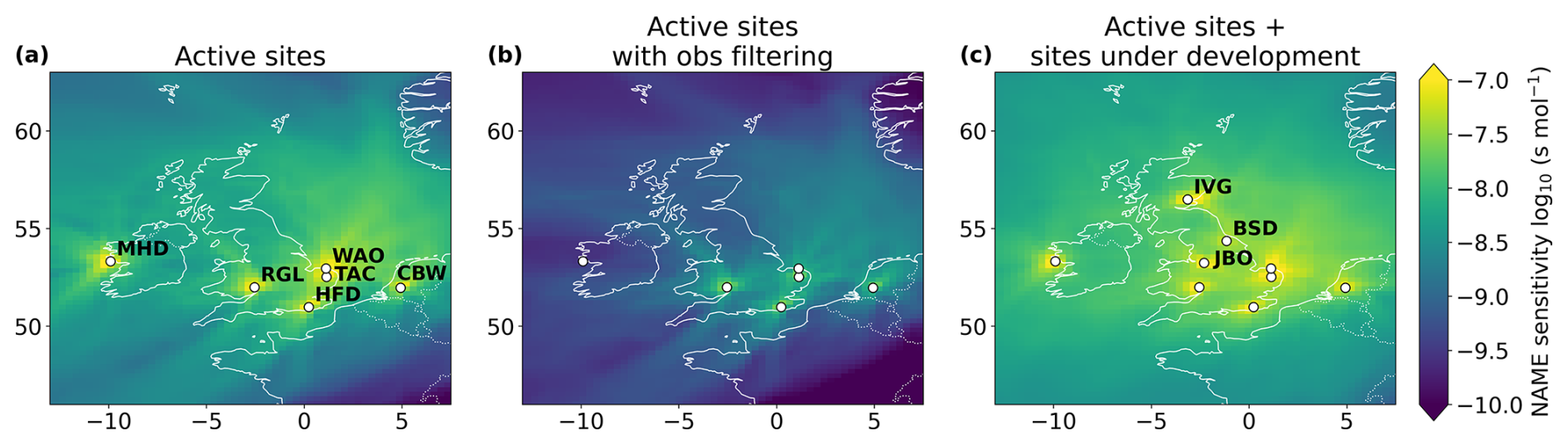
Figure 1 Example months of NAME sensitivity footprints for: (a) May 2023 with all observations from the current network of sites used in this work; (b) May 2023 with observations from the current network, filtered based on meteorological conditions, as used in the UK case study; and (c) May 2024 from the recently expanded network of sites as included in the synthetic study.

Methane δ¹³C-CH₄ and δ²H-CH₄ isotope ratio observations were taken at the HFD site using the “Boreas” preconcentration system coupled to a dual-laser spectrometer (Rennick et al., 2021). Unlike previous methane isotope ratio instruments, which often required weekly flask samples to be transported to a lab for isotopic analysis, this preconcentration system allows for the spectrometer to directly measure mole fractions of ¹²CH₄, ¹³CH₄ and ¹²CH₃D in-situ at high frequency (approximately one hour intervals). These mole fractions were then converted to an isotope ratio. More detail on this instrumentation is available in Rennick et al. (2021) and Safi et al. (2024).

Throughout this work, all observations were averaged into 4-hourly means. This time scale was chosen as a compromise between computation time, suitable variability in emissions and in the model's ability to represent transport and mixing at this resolution.

2.4.2 Transport footprints

Transport footprints, representing the relationship between surface emissions and atmospheric mole fractions, were generated using the Met Office's Numerical Atmospheric-dispersion Modelling Environment (NAME), a Lagrangian particle dispersion model (Jones et al., 2007). With methane's approximately 10-year atmospheric lifetime, it is assumed that loss of methane via chemical reaction is negligible over the 30 d modelling periods. NAME used meteorological fields to simulate the movement of 20 000 inert gas particles from each measurement location back in time for 30 d, recording their interactions with the surface and their exit location from the model domain. NAME was driven by UK-specific 1.5 km horizontal resolution one-hourly temporal resolution meteorological fields over the UK and Ireland and by Unified Model three-hourly resolution fields over the rest of the study domain (Walters et al., 2014). Hourly transport footprints were produced at a spatial resolution of 0.23°×0.35° over the domain of 10.7 to 79.3° N, 97.9° W to 39.7° E. These footprints were then averaged at the same four-hour temporal resolution as the observations. As discussed in Sect. 2.4.5 below, information from the transport footprints on where and when modelled particles exit the study domain were used to create modelled background concentrations.

2.4.3 Observation selection and model-measurement uncertainty

For the UK case study, observations were filtered before use in the inversion. The four-hourly averaged methane observations were filtered to remove times when the air is not well mixed, when we assume that the transport model performs less accurately. Observations were removed if the planetary boundary layer height (as estimated by the Numerical Weather Predication model used to drive the transport model) was within 100 m of the observation height at the observation time. To remove observations with a strong influence from local sources, which can be a sign of poorly-mixed air, data points were also removed if over 15 % of the area-integrated sensitivity at the site was from the 25 grid cells surrounding the site (at the native resolution of the transport footprints). Filtering varied from month to month, but on average these filters removed between 29 % and 38 % of observations from TAC, RGL, HFD and WAO. On average, fewer observations were removed from the MHD, and CBW sites (23 % and 14 %, respectively). Methane isotope ratio observations were then filtered to remove any timestamps without concurrent methane mole fractions observations, as these are required to produce the modelled isotope ratios. On average, 38 % of δ¹³C-CH₄ and δ²H-CH₄ observations were removed before use in each monthly inversion. As an example, Fig. B3 shows the number of observations available before and after filtering for each inversion month at HFD.

Model-measurement uncertainty contains possible sources of uncertainty from the measurements, the model and the representativeness of these two components, including sub-grid cell processes which may impact the 4 h averaged mole fractions but are poorly represented by the model. The standard deviation of the observations within the four-hour averaging period was used to represent the measurement uncertainty. When only one observation was available in the four-hour period, the median uncertainty across the whole month was used. Across all case study months and all sites with available observations, mean measurement uncertainty was 8.15 ppb for methane. δ¹³C-CH₄ and δ²H-CH₄ uncertainties, derived in the same way as for methane, were on average 0.25 ‰ and 1.82 ‰. Model error was included as the maximum of either an optimised scaling factor of the pollution event size at each timestamp, or a pre-defined minimum error (40 ppb for CH₄ and 0.05 ‰ for both δ¹³C-CH₄ and δ²H-CH₄). The pollution event size at each timestamp, for CH₄, δ¹³C-CH₄ and δ²H-CH₄ at each site, was calculated as the difference between the measured value and the modelled baseline, at the current MCMC iteration. A model error scaling factor was optimised for each gas/isotope at each site, for each monthly inversion period. These model error scaling factors were given uniform prior PDFs, between 0 % and 100 % for CH₄ and between 0 % and 50 % for δ¹³C-CH₄ and δ²H-CH₄. The optimised model error scaling factor was applied to the pollution event size, to create the model error used at each timestamp. On average across the case study period and across all sites with available observations, mean model error was approximately 30 % of the posterior methane pollution event size and 22 % for δ¹³C-CH₄ and 24 % for δ²H-CH₄. Combined model-measurement uncertainty for each observation was calculated by taking the root mean square of the measurement uncertainty and the current sample of the model error. The squares of these values (the variances) were then used to fill the diagonal of the model-measurement uncertainty matrix for each species.

2.4.4 A priori emissions and inversion grid setup

An initial (a priori) estimate of annual mean UK emissions from the fossil-fuel (FF) and non-fossil-fuel (non-FF) sectors was taken from the Centre for Ecology and Hydrology (CEH) UK Greenhouse Gas (UKGHG) model of disaggregated UK methane emissions, which is based on nationally reported flux totals (Levy, 2020). For a priori fluxes outside the UK, annual mean flux estimates were taken from the Emissions Database for Global Atmospheric Research (EDGAR) v8.0 (European Commission, Joint Research Centre (JRC), the International Energy Agency (IEA), 2023). Figure 2 shows an example year (2023) of these a priori fluxes and lists the UKGHG and EDGAR sectors that contribute to the aggregated FF and non-FF sectors. In this work, we have not included prior estimates of natural methane fluxes (e.g. from wetlands or freshwater), because in the UK all land is categorised as “managed” and therefore all “natural” sources are included in other sectors. We also do not include emissions from pyrogenic (wildfire) sources, however pyrogenic emissions may have to be considered in future inversions of this type as the wildfire risk in the UK continues to increase (Perry et al., 2022).

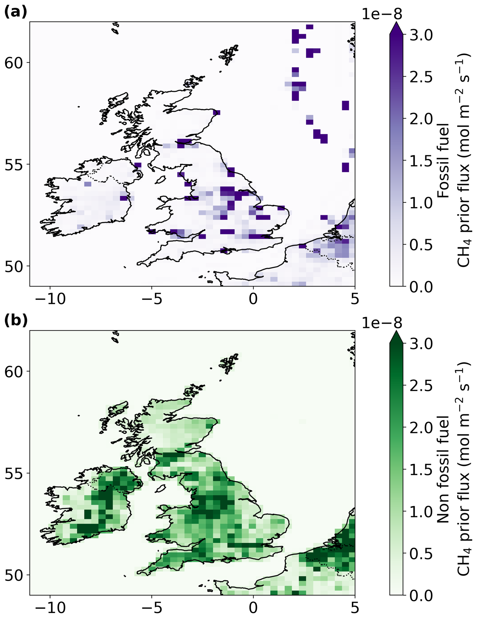
Figure 2 A priori 2023 CH₄ fluxes from CEH's UKGHG model and EDGAR, for the (a) FF and (b) non-FF sectors. The FF prior includes fluxes from domestic and industrial combustion and processes, energy production and use and transport. The non-FF prior includes fluxes from enteric fermentation, manure management, waste water treatments, landfills and waste burning.

In both the synthetic data tests and UK case study, scaling factors of the a priori fluxes were optimised on a lower spatial resolution than the transport footprints or a priori fluxes. For the synthetic data test, only UK emissions were included, so a simple uniform grid of 81 cells was applied over the UK and emissions were estimated over this area. For the UK case study, the whole inversion domain was split into approximately 100 regions, and a scaling factor was optimised for each region. These regions were chosen using a quadtree algorithm, which placed a higher density of smaller regions in areas where there was greater sensitivity to emissions and in areas where prior emissions were higher (see Western et al., 2021 for more detail on this process). This spatial distribution of regions was kept constant throughout the process by using the average sensitivity across all 24 inversion months to inform the quadtree algorithm, enabling a clear comparison of spatial emissions month to month. Before this quadtree algorithm was applied, the outermost areas of the inversion domain, where sensitivity to fluxes is low, was divided into 6 regions. An emissions scaling factor was optimised for each of these larger regions, alongside the approximately 100 smaller regions closer to the study area. Figure 3 gives the two inversion grid setups for the synthetic data test and UK case study.

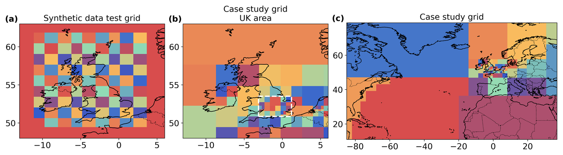
Figure 3 Spatial distributions of optimised regions, used in the (a) synthetic data tests and (b, c) case study. The centre (b) and right (c) plots are identical, with the centre plot a zoomed in section over the UK, showing how the quadtree algorithm places more regions in areas of greater sensitivity to emissions. The dashed white dashed line shows the area over which emissions are estimated during the case study – the south UK area (SUK). This is discussed in Sect. 3.2. Colours used in this plot have no meaning and are just used to differentiate between adjacent regions.

Emission scaling factors were given truncated Gaussian prior PDFs, with means of one and standard deviations of one, equivalent to a 100 % uncertainty on the a priori emissions in each inversion grid cell, truncated at zero to prevent negative emissions.

2.4.5 A priori boundary conditions

A boundary condition scaling factor was optimised for each of the transport model's four domain boundaries, with four values for each inversion month. These higher frequency scaling factors, relative to the monthly emissions, were chosen to account for the seasonal cycles in background methane concentrations. An a priori estimate of mole fractions entering the study domain was created for each North, South, East and West curtain of the study domain. For methane, these a priori boundary conditions were based on the 25th percentile of mole fraction observations each month from the Mace Head (MHD) site, which is situated on the west coast of Ireland and commonly samples background air from across the North Atlantic. When combined with information from the atmospheric transport model, these boundary conditions provided an a priori modelled “background” mole fraction for each observation point used in the study. Boundary condition scaling factors were given Gaussian prior PDFs, with standard deviations leading to equivalent uncertainties in the methane boundary conditions of 2 %.

2.4.6 A priori regional source signatures and boundary isotope ratios

For the synthetic data test and UK case study, regional isotopic signatures for δ¹³C-CH₄ and δ²H-CH₄ for each sector were optimised at different spatial scales, to simulate different levels of uncertainty and variability in these terms. These tests are described in detail in Sects. 2.5 and 3.2 and listed in Tables 2 and 3.

Table 1 Parameters used for the prior regional signature truncated Gaussian PDFs, given as a mean, minimum, maximum and standard deviation (SD).

Table 2 Synthetic data test experiment descriptions, specifying the settings used for each experiment: secondary observations, uncertainty placed on the prior signatures and the number of optimised variables per monthly inversion (degrees of freedom). “Observed” signature uncertainty refers to the source signature datasets discussed in Sect. 2.4.6. x_s are the emissions scaling factors for each sector “s” and x_bc are the boundary condition scaling factors. R_i,s are the region signature scaling factors for each sector “s”, and each isotopologue “i”. R_i,bc are the boundary signature scaling factors and σ are the model error scaling factors, both not included in these experiments.

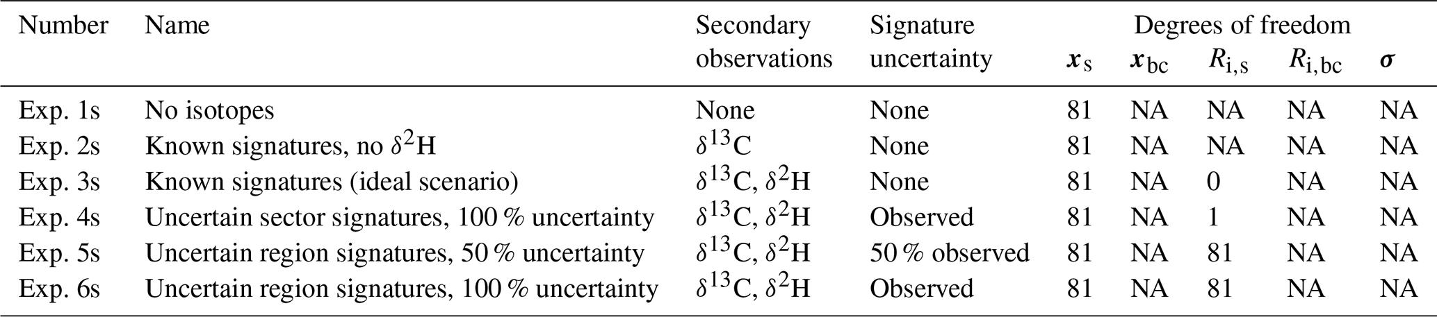
Table 3 UK case study experiment descriptions, specifying the settings used for each experiment: secondary observations, uncertainty placed on the prior source signatures and the number of optimised variables per monthly inversion (degrees of freedom). “Observed” signature uncertainty refers to the source signature datasets discussed in Sect. 2.4.6. x_s are the emissions scaling factors for each sector “s” and x_bc are the boundary condition scaling factors. R_i,s are the region signature scaling factors for each sector “s”, and each isotopologue “i”. R_i,bc are the boundary signature scaling factors and σ are the model error scaling factors, one per site per species.

The means, standard deviations and ranges of the truncated Gaussian regional signature prior PDFs used in each inversion are given in Table 1. They where chosen based on the Royal Holloway database of UK source signatures (Lowry et al., 2020; Menoud et al., 2022) which contains 286 measurements of δ¹³C-CH₄ from a range of sources across the UK: landfill and waste management centres, agricultural ruminants and their waste, gas leaks, mines and roads. These data were combined with a further database of source signatures, compiled during the isoMET project (Dasgupta et al., 2025a, b). Figure B1 presents these data for each source category, as histograms and spatially mapped average signatures, at the resolution of the transport model. Whilst this database does contain information about spatial variation in these signatures, the observed signatures were collected from point sources which may not represent the average signature across a wider area, as optimised by the inversion. Therefore, in this work we used spatially uniform a priori regional signatures, which can be adjusted by the model on a region-by-region basis, in some of the test setups. Data on δ²H-CH₄ source signatures was available from the isoMET database, but was more limited, as shown in Fig. B2.

Boundary condition δ¹³C-CH₄ “signatures”, which represent the average isotopic signature of methane entering the study domain, were given Gaussian prior PDFs, with a mean of −48 ‰ and a standard deviation of 0.5 ‰. These values were based on δ¹³C-CH₄ flask observations at MHD (Michel et al., 2023) which were gathered as part of the National Oceanic and Atmospheric Administration (NOAA) Global Monitoring Laboratory (GML) Carbon Cycle Cooperative Global Air Sampling Network, and analysed at the Institute of Arctic and Alpine Research (INSTAAR) Stable Isotope Laboratory. Boundary condition δ²H-CH₄ signatures were given Gaussian prior PDFs, with a mean of −90 ‰ and a standard deviation of 4 ‰. Independent flask observations of δ²H-CH₄ are not currently taken at MHD, so the average 95th percentile of Boreas observations at HFD was used to inform the δ²H-CH₄ boundary condition prior. As with the methane mole fractions, the influence of δ-values at the boundaries was only considered in the UK case study, not the synthetic data test.

2.5 Synthetic data experiments method

A range of synthetic data tests were carried out to explore the inversion's ability to successfully attribute UK methane emissions to their source categories, using observations from the UK's GHG monitoring network. These tests used observations from six long-established active sites (MHD, TAC, RGL, HFD, WAO and CBW) as discussed above, and three new or reinstated UK sites: the newly-established Scottish Observatory for Atmospheric Research at the Balruddery Research Farm near Invergowrie (IVG) in Scotland (https://blogs.ed.ac.uk/soar/, last access: 6 August 2026); the Jodrell Bank Observatory (JBO) tower, in Cheshire, north-west England; and the Bilsdale (BSD) tall tower site in north-eastern England, which is currently being recommissioned after a fire in 2021. The IVG site currently has a Picarro CRDS instrument to measure methane and an Aerodyne dual laser spectrometer for δ¹³C-CH₄ measurements. In the future, it will have a Medusa GC-MS to measure ethane (amongst many other trace gases) and a Boreas system for δ¹³C-CH₄ and δ²H-CH₄ measurements. JBO has a Picarro CRDS instrument measuring methane, and the BSD site will have a Picarro CRDS instrument when it is reinstated. JBO and IVG have only been running for a short time so do not have the long period of observations required for the UK case study, but have been included in the synthetic tests to demonstrate the potential of the UK network in the near future. Figure 1 shows the locations of the three newly updated sites, with an example month of modelled atmospheric transport footprints.

For these tests, one month of synthetic mole fraction observations were created for each site by combining a priori FF and non-FF flux estimates from the CEH UKGHG methane database (see Sect. 2.4.4) with atmospheric transport footprints (see Sect. 2.4.2). For simplicity, only UK emissions were modelled in these synthetic data tests; boundary conditions and emissions from other areas in the model domain were not used to create the synthetic observations and no background mole fractions were included. To simulate measurement and model error, noise was added to these synthetic observations, proportional to the magnitude of the mole fractions at each site. This prevented the added noise from over-impacting low mole fraction sites (such as MHD and CBW). Added noise was created by scaling the synthetic observations at each site by a randomly sampled value from a Gaussian distribution with a mean of zero and a standard deviation of 0.1. This equated to random noise of between 0 % and 10 % of the synthetic methane observations. Synthetic δ¹³C-CH₄ and δ²H-CH₄ observations were created using steps outlined in Sect. 2.2, with spatially uniform regional signatures of −40 ‰ and −58 ‰ for FF and non-FF sources respectively. These values were chosen based on the Royal Holloway University of London database of UK isotope source signatures as discussed above. Random noise was added to the synthetic isotope ratio observations, using a sampled Gaussian distribution with a standard deviation of 0.05 ‰. Combined model-measurement error was set at the same size as the noise added to each set of synthetic observations. No filtering was applied to the observations, to produce a “best case” scenario, where there was the maximum information available from the observations.

To test whether the inverse system could successfully use these observations to attribute methane fluxes to their two sources, the system was given incorrect a priori flux estimates, created by perturbing the flux fields used to produce the synthetic observations. A successful inversion would be able to produce emissions scaling factors that transformed this perturbed flux prior into the “true” fluxes as contained in the synthetic observations. For each of the 81 inversion grid cells shown in Fig. 3a, the “true” emissions within each cell were scaled by a different value, randomly sampled from a uniform distribution between 0.5 and 1.5. This simulates a scenario where a priori fluxes are up to 50 % incorrect, relative to the fluxes used to produce the observations. The inversion then solved for 81 emissions scaling factors which apply to the whole month, at the same spatial scale as the perturbation field, for each of the FF and non-FF sectors.

Emissions scaling factors were given Gaussian prior PDFs with a standard deviation of 1.0 (equivalent to 100 % uncertainty on the a priori fluxes), truncated at zero preventing negative scaling factors.

The inverse system was run with different combinations of methane isotope ratio observations and prior regional signatures, to simulate a range of scenarios with realistic levels of regional signature uncertainty, considering our current understanding of UK source signatures. All synthetic data experiments (noted by “s” after the experiment number) are summarised in Table 2 and discussed in more detail here:

• Exp. 1s: No isotope observations, only methane mole fraction observations. The inversion could only rely on the spatial distribution within the a priori emissions to infer information about sources.

• Exp. 2s: δ¹³C-CH₄ observations from both HFD and IVG sites, but no δ²H-CH₄ observations. Isotope signatures fixed at the “true” values used to create the synthetic observations. This test simulated a scenario where isotope signatures are known and there is no uncertainty in their values.

• Exp. 3s: Same as Exp. 2s, but with additional δ²H-CH₄ observations from IVG and HFD. Exp. 2s and 3s were run to show the impact of including both types of isotope ratio observations.

• Exp. 4s: δ¹³C-CH₄ and δ²H-CH₄ observations from both sites. One estimated isotope signature per sector. δ¹³C-CH₄ prior mean signatures were created by arbitrarily perturbing the “true” signatures within 100 % of the range of the truncated Gaussian PDFs, as used in the UK case study. This simulated a scenario where there was realistic uncertainty in the signatures for each sector, but no spatial differences in signatures across the UK.

• Exp. 5s: δ¹³C-CH₄ and δ²H-CH₄ observations from both sites. One estimated isotope signature per optimised region per sector. Prior mean signatures for each region were created by randomly perturbing their “true” values within 50 % of the range of the truncated Gaussian PDFs used in the UK case study. This simulated a scenario with spatial variation in signatures across the UK, but only 50 % of the realistic uncertainty in signatures for each sector.

• Exp. 6s: Same as Exp. 5s, but prior mean signatures for each region were created by perturbing the “true” signatures within 100 % of the range of the PDFs used in the UK case study. This simulated a scenario with spatial variation in signatures across the UK and realistic uncertainty in the signatures for each sector.

Each test was repeated 10 times, using 10 different randomly perturbed emission priors and signature priors (where relevant). All repeats used the same example month of transport footprints which showed ideal sensitivity to most areas of the UK from all sites. The differences between the posterior and “true” emissions fields from the 10 repeats of each test were combined using a relative metric, to show where the inversion had made improvements to the emission estimates relative to the prior, where f is the mean emissions from each optimised region:

$$\begin{array}{}\text{(11)}& f={\displaystyle \frac{\text{mean}\left(\right|f_{\text{prior}}-f_{\text{true}}|-|f_{\text{posterior}}-f_{\text{true}}\left|\right)}{\text{mean}\left(\right|f_{\text{prior}}-f_{\text{true}}\left|\right)}}\end{array}$$

3 Results

3.1 Synthetic data experiments

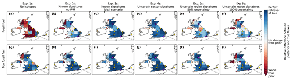
Figure 4 shows the combined results of the synthetic experiments 1s to 6s (left to right), for the FF sector (top row), non-FF sectors (bottom row). Locations of the observation sites used are given as circles, coloured based on the type of observations available at each site.

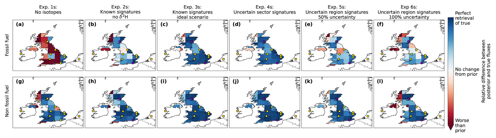
Figure 4 Difference between the posterior and “true” emissions relative to the prior from all synthetic data experiments, for the (top row) FF and (bottom row) non-FF sectors. Results are presented using a relative metric which compares retrieval of the “true” emissions, relative to the prior, as an average from all 10 repeats of each experiment (Eq. 11). Dark blue areas show a perfect retrieval of the “true” fluxes, white areas show no change from the prior and red areas show emission estimates that are further away from the truth than the prior. Results are given for Experiments 1s–6s as described in Table 2. Coloured dots show observation locations for: only CH₄ (yellow) and CH₄ and CH₄ isotope ratios (purple).

The methane-only experiment (Exp. 1s, Fig. 4a, g) was unable to replicate the true FF emissions for the majority of the UK. There is some accurate estimation of non-FF emissions across England, Wales and eastern Scotland. The methane-only experiment may have been able to correctly replicate emissions in these areas because of the relatively limited contribution of the FF sector (see Fig. 2), therefore the inversion was effectively performing a single-sector inversion in these areas. In all experiments, both the relative size of emissions from each sector and the sensitivity to emissions across different areas of the UK likely impacted the results. For example, in western Scotland where sensitivity is relatively poor (see Fig. 1), and emission from both sectors is low (see Fig. 2) the model could produce large perturbations from the “true” emission, without a strong impact on the modelled mole fractions. The impact of sensitivity and emission magnitude should be considered in the following qualitative analysis of the synthetic data test results.

Most of the synthetic experiments including isotopic data (2s–6s) yield an improved estimate of the “true” emissions fields over much of the UK compared to the methane-only experiment. However, the spatial extent of this success and the ability to accurately estimate emissions from both sectors depends on the observations used and the regional signature uncertainty.

Fixing regional signatures at the “true” values (those used to produce the synthetic observations) produced the most accurate estimates of FF and non-FF emissions. In experiment 3s, when synthetic observations of both δ¹³C-CH₄ and δ²H-CH₄ (Fig. 4c, i) were included, emissions are estimated correctly for both sectors, apart from the most north-west of Scotland, where there are still some inaccuracies in non-FF emissions estimates. In experiment 2s, when only δ¹³C-CH₄ observations were included (Fig. 4b, h), there are only small changes from the prior in the FF sector for most areas and there are some inaccuracies in non-FF emissions in western UK, where emission sensitivity is lower. Following this result, the additional synthetic experiments (4s–6s) were only carried out with both δ¹³C-CH₄ and δ²H-CH₄ synthetic observations.

The tests with a perturbed regional signature prior per sector (Exp. 4s) simulate a scenario in which we assume a single signature per sector with some uncertainty but without any spatial variation (i.e. a single signature applies to the whole of the UK for each sector). The synthetic data test with this setup (Exp. 4s, Fig. 4d, j) was as successful as that with fixed regional signatures (Exp. 3s, Fig. 4c, i) and the model was able to adjust the perturbed regional signatures back to their “true” values, reproducing both the “true” emissions fields and modelled isotope ratios.

The tests with perturbed regional signature priors at the same spatial resolution as the emissions scaling factors, with no assumption that the signatures are uniform over the whole country (Exp. 5s and 6s) show the limitations of this method. When the prior mean regional signatures are within 50 % of the current, observed, uncertainty in these signatures (Exp. 5s, Fig. 4e, k) the model is able to adjust these perturbed signatures back to their “true” values with some success and correctly estimate non-FF emissions over most of the UK. Emission estimates for the FF sector show strong improvement on the methane only test (Exp 1s, Fig. 4a, g), but there are some inaccuracies (lack of movement from the prior) in the emissions, especially in areas where the sensitivity to emissions is lower; for example, away from HFD in the south-east and IVG in the north. When prior mean regional signatures are perturbed further, falling anywhere within the full range of the current uncertainty in these signatures (Exp. 6s, Fig. 4f, l), posterior emission estimates become less accurate; non-FF emission estimates are similar to those from the methane-only inversion (Exp. 1s, Fig. 4a, g) and there is little movement from the prior in central England, where sensitivity at HFD and IVG is poor. This result highlights the risks of including regional signatures with high uncertainties in the model; there are many degrees of freedom and the model can adjust any of these parameters freely within prior uncertainties in order to produce the best fit to the observations. If emissions and signatures are not well constrained by the observations, this can lead to inaccurate emissions estimation and shows limited benefit, when compared to the methane-only inversion.

Overall, these results suggest that accurate estimation of whole-UK FF and non-FF emissions could be possible by using δ¹³C-CH₄ and δ²H-CH₄ observations from the HFD and IVG sites, when regional signatures are well understood (i.e. have low uncertainty) and the signatures have either no or only limited spatial variation. In reality, as the spatial and temporal differences in signatures across the UK are not well understood, we have to allow the inversion to consider all possible signature values across the UK when looking for an optimised estimate of emissions. This introduces a large number of degrees of freedom (as shown in Table 2) which the limited isotope observations struggle to constrain. This is discussed in more detail in Sect. 3.2.

Importantly, the synthetic data tests described above used an idealised scenario with low model and observational uncertainties and consistently available high frequency observations from multiple observation sites. In a real-world scenario, all three aspects will be challenged to a greater or lesser degree.

3.2 Real-world UK methane emissions case study

The synthetic data test results presented above show that the described inverse modelling system could potentially be used with methane isotope ratio observations to directly estimate sector-level UK methane emissions. However, these were idealised scenarios, which: included no impact from background concentrations; no emissions from western Europe; assumed accurate transport modelling and included observations from recently established or soon-to-be established sites that do not currently have a long history of observations.

To test these findings in a real-world scenario, we applied the inverse method to estimate monthly methane emissions from the FF and non-FF sectors from January 2022 to December 2023. We used δ¹³C-CH₄ and δ²H-CH₄ Boreas observations from HFD, alongside methane mole fraction observations from MHD, TAC, RGL, HFD, WAO and CBW. Table 3 gives the six experiments with different combinations of secondary observations and isotope signature setups (with “r” referring to real data). These experiments aim to replicate those used in the synthetic data tests discussed above, but also include additional degrees of freedom and uncertainty from the boundary conditions and model error scaling factors.

As Fig. 1b and the synthetic data tests showed, good isotopic sensitivity to emissions is limited to the south-east of the UK by the location of currently available isotope ratio observations. Therefore, we only estimate emissions and analyse results over this area of good sensitivity. This region is shown by the dashed white rectangle in Fig. 3, and is henceforth referred to as south UK (SUK).

All results are analysed relative to those from the methane-only inversion, in order to determine whether the additional observations provide greater constraint on FF and non-FF methane fluxes than a traditional single-gas inversion which is only constrained by spatial information in the a priori emissions. Total emissions estimates from each sector are discussed in more detail below. First, the inverse systems' ability to produce modelled isotope ratios is demonstrated.

3.2.1 Modelled isotope ratios

Figure 5 shows posterior modelled methane model fractions and isotope ratios from the HFD site, from Experiment 6r: with observations of both types of isotope ratio and variable regional signatures at the same spatial resolution as the emissions scaling factors. Results are shown for two example months (August and September 2023) which show the best observational coverage of all months in the two year study period. Comparison between observations and modelled isotope ratios shows a good fit at most timestamps, other than when excursions away from baseline are extreme or when the measurement uncertainty (within a given 4 h period, as discussed in Sect. 2.4.1) is very large (as shown by error bars on the observations). The average RMSE and Pearson correlation coefficients and histograms giving the difference between observed and modelled isotope ratios (Fig. 5, panels b, d) show how the model has effectively adjusted modelled isotope ratios away from their priors and closer to the observations. The model has adjusted both the boundary “signatures” (as shown by adjustments in the baseline) and the methane emission and boundary condition scaling factors (as shown by a closer match between modelled isotope ratios and observations).

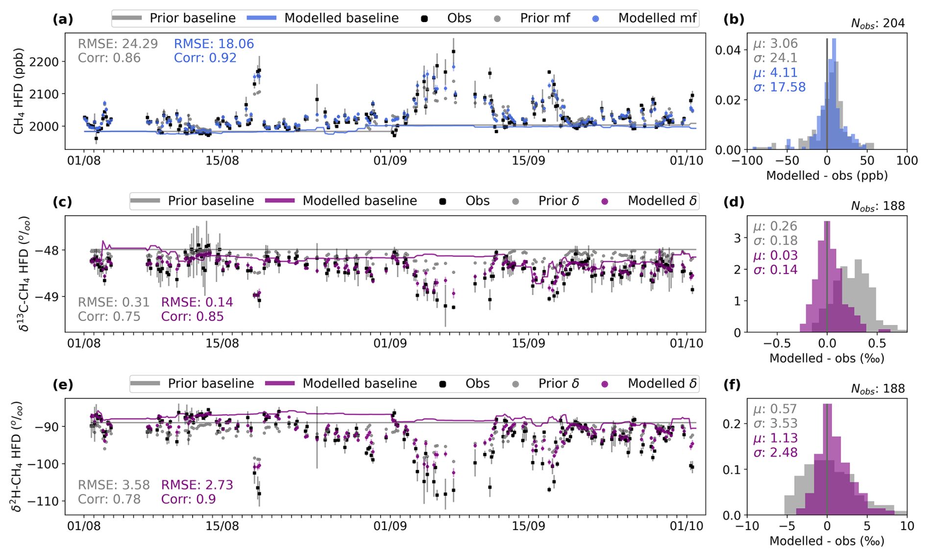
Figure 5 Modelled mole fractions and isotope ratios from Experiment 6r of the UK case study: with isotope ratio observations from the HFD site and variable regional signatures at the same spatial resolution as the emissions scaling factors. Four-hourly averaged observations (black squares) of (a) CH₄ mole fractions, (c) δ¹³C-CH₄ and (e) δ¹³C-CH₄ δ-values from the HFD site, for two example months August to September 2023. These are compared against (blue or purple colour) posterior modelled values and (grey) prior modelled values from the inversion with variable regional signatures. Differences between the observations and the prior and posterior modelled mole fractions and δ-values are given on the right, as histograms. The mean (μ) and standard deviations (σ) of these model-observation differences are also given. The RMSE and Pearson correlation coefficient of the observed and modelled values is given in the top left of each figure for the (grey) prior and (blue or purple) posterior. (Grey line) prior and (blue or purple line) posterior mean baselines are also shown for comparison.

Figure B5 shows the bias, RMSE and correlation between posterior mean and observed mole fractions and isotope ratios at the HFD site, for all case study experiments. These statistics show that the inversions' ability to model isotope ratios which match observations does not change substantially when increasing the uncertainty given to isotope signatures (Experiments 4r to 6r). However, fit to the observations worsens when assuming fixed signatures with no spatial variation (Experiments 2r and 3r). From this, we can conclude that assuming fixed signatures per sector will not allow the inversion to produce the best possible estimate of FF and non-FF emissions.

When using signatures fixed at their prior means (Experiments 2r and 3r), the residuals between modelled and observed isotope ratios increase when compared to those from experiments using variable regional signatures. Figure B4, which gives the modelled mole fractions and isotope ratios from Experiment 3r, shows that modelled δ¹³C-CH₄ have not moved significantly from their priors. The difference between modelled and observed δ²H-CH₄ decreases when using variable regional signatures, however even the inversion with fixed signatures shows some improvement on modelled δ²H-CH₄, relative to the prior. The different impact of variable regional signatures on each type of methane isotope ratio could be due to the relative size of δ¹³C-CH₄ and δ²H-CH₄ excursions away from the baseline or could be due to the nature of the two observation types: δ¹³C-CH₄ excursions away from the baseline can be either positive or negative depending on the source type. When a mixture of FF and non-FF sources impact the mole fraction, the resulting δ¹³C-CH₄ isotopic signature could be similar to that of the atmospheric background. Whereas, δ²H-CH₄ excursions away from the baseline are always negative, with the most negative values characteristic of biogenic (non-FF) sources. Smaller changes in FF and non-FF emissions scaling factors may therefore have a larger impact on the modelled δ²H-CH₄ than the modelled δ¹³C-CH₄.

3.2.2 Modelled regional and spatial emissions

Figure 6 shows each experiment's posterior estimate of SUK FF and non-FF methane emissions, as combined averages from all monthly inversions between January 2022 and December 2023. Results are presented as averages because the limited study period prevented any analysis of trends or seasonal cycles. The spread of these monthly results are presented using two metrics: the standard deviation of the posterior monthly means (smaller uncertainty bar) and the RMSE of the posterior uncertainty bounds from each monthly inversion (larger uncertainty bar). The RMSE term presents the full range of possible solutions for emission estimates from all monthly inversions, which could include both uncertainty in the inversion estimates and any potential seasonal cycle in emissions across the two years.

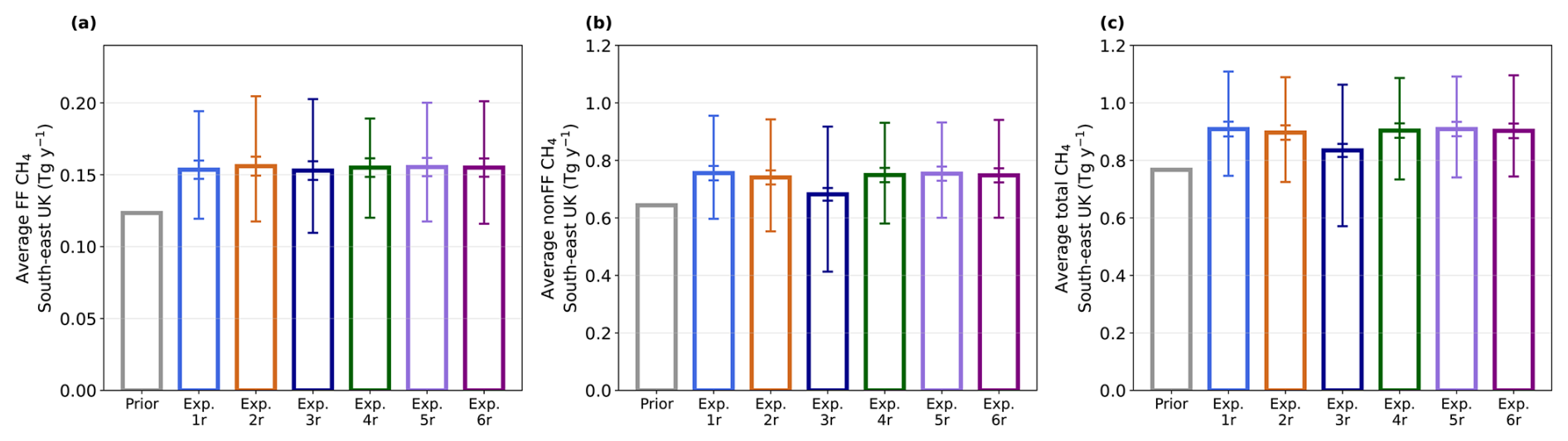
Figure 6 Posterior CH₄ flux estimates for the SUK area (as shown in Fig. 3) averaged across all 2022–2023 study months. Results for the (a) FF sector, (b) non-FF sector and (c) all sources, for the six different case study experiments are presented as a posterior mean across all months. With (narrower error bar) 1σ uncertainty of these posterior means and (wider error bar) RMSE of the posterior standard deviations across all monthly emission estimates. Descriptions for each experiment are given in Table 3.

Within posterior uncertainties, there are no significant differences in the magnitude of mean posterior emissions estimates for the FF sector, from all experiment setups. However, the full range of uncertainty (RMSE) in FF emission estimates increases from Exp. 1r to 3r as more isotope observations (with their own associated uncertainties) are included in the system. This uncertainty reduces once the inversion is allowed to adjust isotopic signatures (Exp. 4r) but increases again as more uncertainty is given to the isotopic signatures (Exp. 5r and 6r).

Results from all experiments for the non-FF sector show similar patterns to those from the FF sector, except for two differences. Firstly, the average non-FF emission estimate lowers by approximately 9 % when using fixed isotope signatures (Exp. 3r), compared to the other experiments. This lowering of emissions from the non-FF sector is not coupled with an increase in FF emissions, so estimates of total emissions also decrease, within the high level of prior uncertainty in this two-sector inversion. This result, combined with the conclusions discussed above about Experiment 3r's ability to model isotope ratios at HFD, highlights that care must be taken when assuming spatially and temporal invariant source signatures. Secondly, increasing isotopic signature uncertainty (from Exp. 4r to 6r) does not have as significant an impact on the spread of possible non-FF emission estimates compared to the FF emission estimates. This could be due to the relative contribution of the two sectors to total emissions: the model may allow for more variation in the FF sector within prior and observational uncertainties, because of its smaller impact on the total emission estimates.

Overall, average posterior uncertainty remains high from all experiments: mean posterior standard deviation is 18 % and 14 % for the FF and non-FF sectors. A relatively high uncertainty is to be expected from the methane-only experiment (Exp. 1r), where only the spatial distribution and magnitude of emissions in the prior provide constraint on the posterior sector split. The isotope ratio observations' limited ability to reduce posterior uncertainty is discussed in more detail in Sect. 4.

Mean average spatial emissions estimates from all experiments (1r to 6r) for the whole study period are given in Fig. 7. Emissions from the methane-only inversion (Exp. 1r) are given as scaling factors of the prior mean emission for the FF and non-FF sector. Emission estimates from the experiments with secondary observations are given as absolute differences in posterior scaling factor, relative to the methane-only experiment, to better show the minor differences in results.

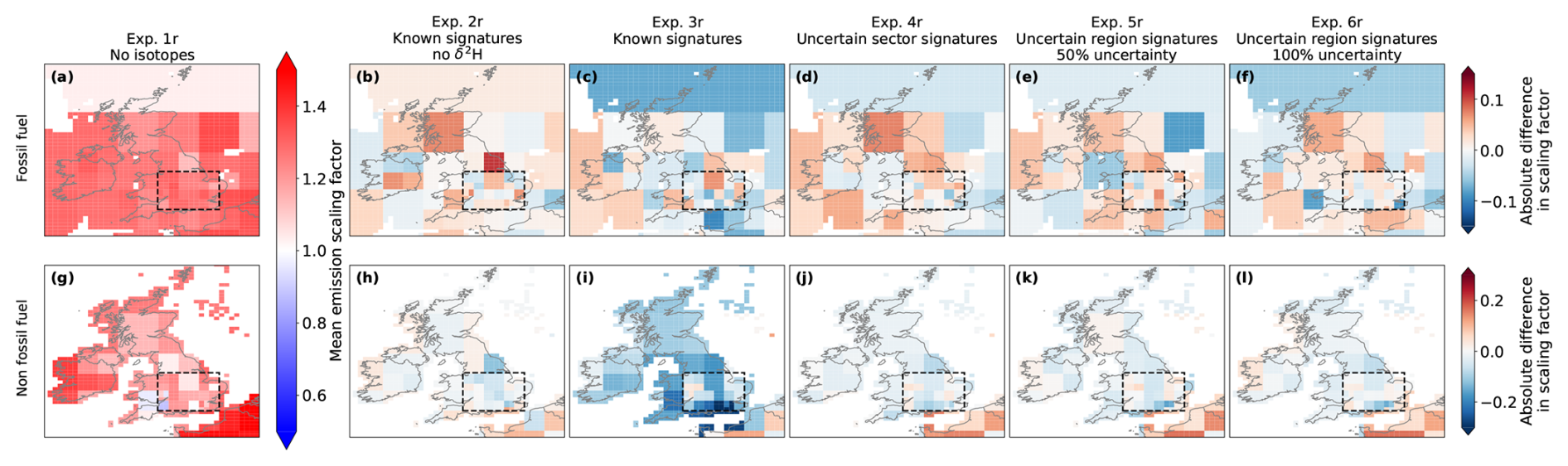
Figure 7 Average posterior mean monthly flux estimates for UK across all study months (2022–2023) for the FF sector (top row) and non-FF sector (bottom row) from all case study experiments, as described in Table 3. Dashed lines show the SUK area, over which results are analysed. CH₄-only results (Exp. 1r, panels a, g) are shown as absolute differences from the prior emissions estimates. Results from all other experiments are given as absolute differences from this CH₄-only posterior-prior difference.

On average across this period, the methane-only setup (Exp. 1r) slightly increased estimates of FF emissions across the SUK area (outlined box), relative to the prior. From all experiments with isotope observations, there are no consistent strong differences in FF emission across the whole SUK area, compared to the methane-only setup, apart from a minor increase in emissions in central England. As uncertainty on the isotope signatures increases (from Exp. 3r to 6r) the adjustment of average posterior FF emissions, relative to the methane-only setup (Exp. 1r) reduces. This implies that the inversion may be adjusting signatures instead of adjusting emissions, within their increasing uncertainty, to produce a better fit to the observations.

For the non-FF sector, the methane only setup (Exp. 1r) shows a general positive scaling of emission relative to the prior in some but not all areas, and shows more regional variation than the FF sector. Most experiments with isotope observations (Exp. 2r, 4r, 5r, 6r) show minor reductions in non-FF emission scaling factors, relative to the methane-only setup, in south-east England near London and near the HFD observation site. This relative reduction in non-FF emissions is strongest for Exp. 5r and 6r which include higher uncertainty in the isotopic signatures. Using signatures fixed at their prior and observations of both δ¹³C-CH₄ and δ²D-CH₄ (Exp. 3r) strongly reduces the inversion's estimate of non-FF emissions, relative to the methane-only setup, in southern and central England. As discussed above, this suggests that the inversion may be lowering emissions in an attempt to counter potentially incorrect prior isotope signatures.

Using spatial emission estimates averaged over two years is limiting our ability to drawn useful conclusions about the isotope observations' impact on spatial emissions. Especially as methane is known to show some seasonal variation in emission, which may be masking any clear impact of the isotope observations on emissions in this multi-year average. However, longer time-series of observations would be required in order to analyse spatial emission results at monthly or seasonal resolution. This expanded analysis is planned for future work, when more years of observations become available.

Table 4 gives the posterior signatures from each experiment with variable signatures, as averages across all inversion months. Posterior uncertainty in signatures remains high, although there is some reduction relative to the prior uncertainty (see Table 1). This narrowing of posterior signature uncertainty suggests that signatures at the more extreme ends of the prior PDFs are not required in order to produce a good fit to observations, in an inversion at this spatial resolution where most regions contain a mixture of sources with a combined less-extreme signature. This conclusion is supported by the narrower average signatures estimated by Exp. 5r, which used signature prior PDFs with 50 % less uncertainty than other experiments but produced modelled isotope ratios similar to those from the other experiments. We found no relationship between posterior mean signatures and posterior mean emission scaling factors across the SUK area, showing that individual emission estimates are not being strongly biased by adjustments to the signatures. However, this result and the wide range of posterior regional signatures produced by the inversions suggests that the model may be adjusting regional signatures within their prior uncertainties, to produce modelled isotope ratios with a better fit to the observed isotope ratios, rather than adjusting emissions. Posterior boundary “signatures” are similar for all model setups, with posterior means (minimum, maximum) of −48.0 ‰ (−49.1 ‰, −47.1 ‰) and −88.4 ‰ (−98.9 ‰, −77.1 ‰) for δ¹³C-CH₄ and δ²H-CH₄. The lowest boundary signatures were estimated for the southern boundary of the inversion domain, which receives air that has recently passed over western Europe.

Table 4 Average source and boundary signatures from the case study experiments with variable signatures. Results are given as the posterior mean and minimum and maximum of the posterior PDFs across all inversion months, to show the full uncertainty in these values. For the experiments with one signature per sector per region (Exp. 5r and 6r), posterior PDFs are only included for regions within the SUK area.

4 Discussion

These case study experiments have shown that using the inverse system with uncertain source signatures and methane isotope ratio observations from one site produces estimates of SUK FF and non-FF emissions with no strong differences when compared to results from a methane-only inversion. This could be due to a range of factors. Firstly, the prior estimate of emissions from each sector could be accurate and require no adjustment to produce modelled mole fractions and isotope ratios which are a good fit to atmospheric observations. If this was the case, additional information from the isotope ratio observations would not impact the inversions' emissions estimates, relative to what the methane-only setup achieves. Alternatively, the isotope ratio observations may not be able to provide any greater constraint on emissions because there is a relative lack of information from the isotope observations (from only one site) compared to that from the mole fraction observations (six sites) and uncertainties from the constraining parameters (regional signatures) may be too high. These two limiting factors are discussed in more detail below.

The synthetic data tests showed that the inversion was most effective at estimating FF and non-FF emissions with uncertain regional signatures when there was only one signature per emissions sector (Exp. 4s). However, the real-world test of this scenario (Exp. 4r) estimated emissions similar to those from the methane-only setup. This could suggest that in reality there is some spatial variation in source signatures which cannot be captured by this setup, and therefore this restriction is limiting the additional observations' ability to impact posterior emissions uncertainty. However, when including spatial variation in the signatures (Exp. 5r and 6r) the number of degrees of freedom and overall uncertainty in the inversion increases significantly, whilst the constraint from the limited number of isotope observations is unchanged. The synthetic data tests used isotope ratio observations from two sites, compared to the single site used for the UK case study. To compensate for this, we analysed the case study results over the SUK region where the HFD site has good sensitivity to emissions. However, results over this region do not vary significantly from those from the methane-only setup, potentially suggesting that even more isotope ratio observations are required to provide enough information to better constrain sector-level emissions across any area of the UK.

Previous work showed that incorporating ethane observations into the inversion was a more effective method for reducing the inversion's uncertainty in posterior FF fluxes (Ramsden et al., 2022). Ethane's greater impact on FF flux uncertainty could be due to a range of factors: higher density of ethane observations; location of these ethane observations and their sensitivity to UK-wide emissions; or lower relative uncertainty in ethane:methane emission ratios compared to the uncertain isotopic signatures included in this work. Combining both ethane mole fraction and methane isotope ratio observations in the inversion could provide an even greater constraint on emissions, despite the increased prior uncertainties involved with including additional observations and ethane:methane emission ratios. This will be explored in future work.

The nature of methane isotope source signatures may also be limiting the model's ability to use the additional information from methane isotope ratio observations to reduce regional posterior flux uncertainty. In this work, emissions are optimised over relatively coarse regions, which can contain multiple different methane sources. The resulting isotopic signature from each region will be an average from all these sources (a “regional signature”). Any signal from elevated emissions from one source (“pollution events”) may be lost in the averaged isotopic signature from all sources in that region. This could reduce the information available from the methane isotope ratio observations.

Improved understanding of methane isotope source signatures, or improved incorporation of our current understanding into the inversion, is a key focus for future development of this method. Currently, this inversion system assumes a two-sector setup with a large uncertainty in source signatures from the non-FF sector and no spatial information in the signature priors. However, information on the spatial and temporal distribution of agriculture and waste sources (which both contribute to the non-FF sector) could be used to produce a non-FF signature prior with spatial information. This would better inform the modelled isotope ratios and reduce prior uncertainty in some regions. Alternatively, a three-sector inversion could be carried out, assuming that agriculture and waste sectors have distinct source signatures. However, such a system could potentially assign emissions inaccurately to each of the agriculture or waste sectors, whilst still producing FF emissions estimates with lower uncertainty. Also, currently, we assume no spatial or temporal correlations in emissions or source signatures. Inclusion of these correlations could limit the model from over-adjusting signatures locally, where it is assumed that emissions sources will be similar; this might allow for greater constraint on emissions.

Without greater understanding of isotopic source signatures and a higher density network of isotope observations, the method was not able to provide substantial constraints on regional FF and non-FF fluxes, beyond that obtained from a mole fraction only inversion.

5 Conclusions

This work has presented a novel inverse modelling method that is highly adaptable and can be used with a range of secondary observations to directly estimate emissions from two (or more) sectors concurrently. The inversion uses the relationship between observations of its primary gas, in this case methane, to secondary isotope ratio observations via regional isotopic signatures. By including both the uncertainties and spatial and temporal differences in isotopic source signatures, this work builds on previous isotope inversion methods with the aim of reducing the uncertainty in the posterior flux estimates of the FF and non-FF sectors.

Synthetic data tests, considering a range of uncertainties in the methane isotope regional signatures, have shown that the inversion can accurately estimate UK methane emissions from both FF and non-FF sectors. The synthetic data inversion performed best when regional isotopic signatures were well understood or had low uncertainty. In high-uncertainty scenarios, estimates of emissions became less accurate, particularly for the FF sector.

New δ¹³C-CH₄ and δ²H-CH₄ observations from the Heathfield (HFD) site in southern England were used to estimate monthly FF and non-FF methane fluxes for a region in the south-east UK between 2022 and 2023. The scenarios with methane isotope ratio observations produced similar estimates of FF and non-FF emissions to those from the methane-only setup, apart from experiments where regional signatures were fixed at their priors. In this scenario, the fit to the isotope observations worsened and non-FF emissions were lowered relative to the methane-only setup, which could indicate that the prior isotope source signatures used in this case were not fully representative. The results from all tests of the method lead us to conclude that the lack of impact on emissions uncertainty in the experiments with variable signatures is because current UK methane isotope ratio observations are too limited and the uncertainties in isotopic source signatures are too high to provide strong additional constraint on emissions. This is an important result which provides clear evidence for the need to continue the ongoing expansion of the observational network and improved quantification of source signatures.

Options for further development of this method include the use of more informative source signature priors, with more spatial variation and reduced uncertainty, which could be provided by expanded source signature observation campaigns. Considering spatial and temporal correlations in regional signatures or reducing the resolution at which signatures are optimised in the inversion could further reduce the prior uncertainty of these terms. Alternatively, additional secondary observations, such as ethane, could be incorporated alongside the methane isotope observations for greater constraint on the FF emissions estimates.

Two recent Horizon Europe research projects (Process Attribution of Regional Emissions (PARIS) and the Metrology for European emissions verification on methane isotopes (isoMET) project) focused on expanding European networks of methane isotope ratio and ethane observations and improving our understanding of the source signatures of methane's sources. Work presented here shows that with this continued investment in reliable long-term networks of secondary observations, this inverse modelling method has the potential to provide an independent evaluation of the UK and Europe's bottom-up flux estimates from fossil-fuel and non-fossil-fuel sectors. This independence will become a key component of effectively monitoring trends in the UK and Europe's methane emissions in the future, as emissions targets and reporting requirements become more stringent and the mix of methane sources changes.

Appendix A: Calculating isotopologue absolute fractions

This method assumes that there are only three methane isotopologues present in the atmosphere: ¹²CH₄, ¹³CH₄ and ¹²CH₃D. The total methane mole fraction can be found by summing the contributions from each isotopologue:

$$\begin{array}{}\text{(A1)}& {\mathrm{CH}}_{\mathrm{4}}={}^{\mathrm{12}}{\mathrm{CH}}_{\mathrm{4}}+{}^{\mathrm{13}}{\mathrm{CH}}_{\mathrm{4}}+{}^{\mathrm{12}}{\mathrm{CH}}_{\mathrm{3}}\mathrm{D}\end{array}$$

The absolute mole fraction of each isotopologue can be found by considering the ratio of isotopologues given by isotope ratio observations and substituting this information into Eq. (A1).

Methane isotope ratio observations are presented as delta values:

$$\begin{array}{}\text{(A2)}& {\mathit{\delta }}_{\text{i}}=\left({\displaystyle \frac{R_{\text{i}}}{R_{{\mathrm{std}}_{\mathrm{i}}}}}-\mathrm{1}\right)\end{array}$$

where R_i for the two sets of methane isotope observations used in this work are:

$$\begin{array}{}\text{(A3)}& {\displaystyle }{\mathit{R}}_{\mathrm{13}}={\displaystyle \frac{{}^{\mathrm{13}}{\mathrm{CH}}_{\mathrm{4}}}{{}^{\mathrm{12}}{\mathrm{CH}}_{\mathrm{4}}}}\text{(A4)}& {\displaystyle }{\mathit{R}}_{\mathrm{2}}={\displaystyle \frac{{}^{\mathrm{12}}{\mathrm{CH}}_{\mathrm{3}}\mathrm{D}}{{}^{\mathrm{12}}{\mathrm{CH}}_{\mathrm{4}}}}\end{array}$$

To find the absolute fraction of ¹²CH₄, Eqs. (A3) and (A4) are rearranged then substituted into Eq. (A1):

$$\begin{array}{}\text{(A5)}& \begin{array}{rl}& {}^{\mathrm{13}}{\mathrm{CH}}_{\mathrm{4}}={}^{\mathrm{12}}{\mathrm{CH}}_{\mathrm{4}}{\mathit{R}}_{\mathrm{13}}\\ & {}^{\mathrm{12}}{\mathrm{CH}}_{\mathrm{3}}\mathrm{D}={}^{\mathrm{12}}{\mathrm{CH}}_{\mathrm{4}}{\mathit{R}}_{\mathrm{2}}\\ & ⟹{\mathrm{CH}}_{\mathrm{4}}={}^{\mathrm{12}}{\mathrm{CH}}_{\mathrm{4}}+{}^{\mathrm{12}}{\mathrm{CH}}_{\mathrm{4}}{\mathit{R}}_{\mathrm{13}}+{}^{\mathrm{12}}{\mathrm{CH}}_{\mathrm{4}}{\mathit{R}}_{\mathrm{2}}\\ & ⟹{\mathrm{CH}}_{\mathrm{4}}={}^{\mathrm{12}}{\mathrm{CH}}_{\mathrm{4}}\left(\mathrm{1}+{\mathit{R}}_{\mathrm{13}}+{\mathit{R}}_{\mathrm{2}}\right)\\ & ⟹{}^{\mathrm{12}}{\mathrm{CH}}_{\mathrm{4}}={\displaystyle \frac{{\mathrm{CH}}_{\mathrm{4}}}{\left(\mathrm{1}+{\mathit{R}}_{\mathrm{13}}+{\mathit{R}}_{\mathrm{2}}\right)}}\end{array}\end{array}$$

The absolute fractions of ¹³CH₄ and ¹²CH₃D can then be derived from Eq. (A5) by substituting in Eqs. (A3) and (A4):

$$\begin{array}{}\text{(A6)}& \begin{array}{rl}{}^{\mathrm{12}}{\mathrm{CH}}_{\mathrm{4}}& ={\displaystyle \frac{{\mathrm{CH}}_{\mathrm{4}}}{\left(\mathrm{1}+{\mathit{R}}_{\mathrm{13}}+{\mathit{R}}_{\mathrm{2}}\right)}}\\ & ⟹{\displaystyle \frac{{}^{\mathrm{13}}{\mathrm{CH}}_{\mathrm{4}}}{{\mathit{R}}_{\mathrm{13}}}}={\displaystyle \frac{{\mathrm{CH}}_{\mathrm{4}}}{\left(\mathrm{1}+{\mathit{R}}_{\mathrm{13}}+{\mathit{R}}_{\mathrm{2}}\right)}}\\ & ⟹{}^{\mathrm{13}}{\mathrm{CH}}_{\mathrm{4}}={\displaystyle \frac{{\mathit{R}}_{\mathrm{13}}{\mathrm{CH}}_{\mathrm{4}}}{\left(\mathrm{1}+{\mathit{R}}_{\mathrm{13}}+{\mathit{R}}_{\mathrm{2}}\right)}}\\ & ⟹{}^{\mathrm{13}}{\mathrm{CH}}_{\mathrm{4}}={\displaystyle \frac{{\mathrm{CH}}_{\mathrm{4}}}{\left(\frac{\mathrm{1}}{{\mathit{R}}_{\mathrm{13}}}+\mathrm{1}+\frac{{\mathit{R}}_{\mathrm{2}}}{{\mathit{R}}_{\mathrm{13}}}\right)}}\end{array}\end{array}$$

$$\begin{array}{}\text{(A7)}& \begin{array}{rl}{}^{\mathrm{12}}{\mathrm{CH}}_{\mathrm{4}}& ={\displaystyle \frac{{\mathrm{CH}}_{\mathrm{4}}}{\left(\mathrm{1}+{\mathit{R}}_{\mathrm{13}}+{\mathit{R}}_{\mathrm{2}}\right)}}\\ & ⟹{\displaystyle \frac{{}^{\mathrm{12}}{\mathrm{CH}}_{\mathrm{3}}\mathrm{D}}{{\mathit{R}}_{\mathrm{2}}}}={\displaystyle \frac{{\mathrm{CH}}_{\mathrm{4}}}{\left(\mathrm{1}+{\mathit{R}}_{\mathrm{13}}+{\mathit{R}}_{\mathrm{2}}\right)}}\\ & ⟹{}^{\mathrm{12}}{\mathrm{CH}}_{\mathrm{3}}\mathrm{D}={\displaystyle \frac{{\mathit{R}}_{\mathrm{2}}{\mathrm{CH}}_{\mathrm{4}}}{\left(\mathrm{1}+{\mathit{R}}_{\mathrm{13}}+{\mathit{R}}_{\mathrm{2}}\right)}}\\ & ⟹{}^{\mathrm{12}}{\mathrm{CH}}_{\mathrm{3}}\mathrm{D}={\displaystyle \frac{{\mathrm{CH}}_{\mathrm{4}}}{\left(\frac{\mathrm{1}}{{\mathit{R}}_{\mathrm{2}}}+\frac{{\mathit{R}}_{\mathrm{13}}}{{\mathit{R}}_{\mathrm{2}}}+\mathrm{1}\right)}}\end{array}\end{array}$$

These terms can then used to produce modelled atmospheric methane isotope ratios as described in Sect. 2.2.

Appendix B: Figures

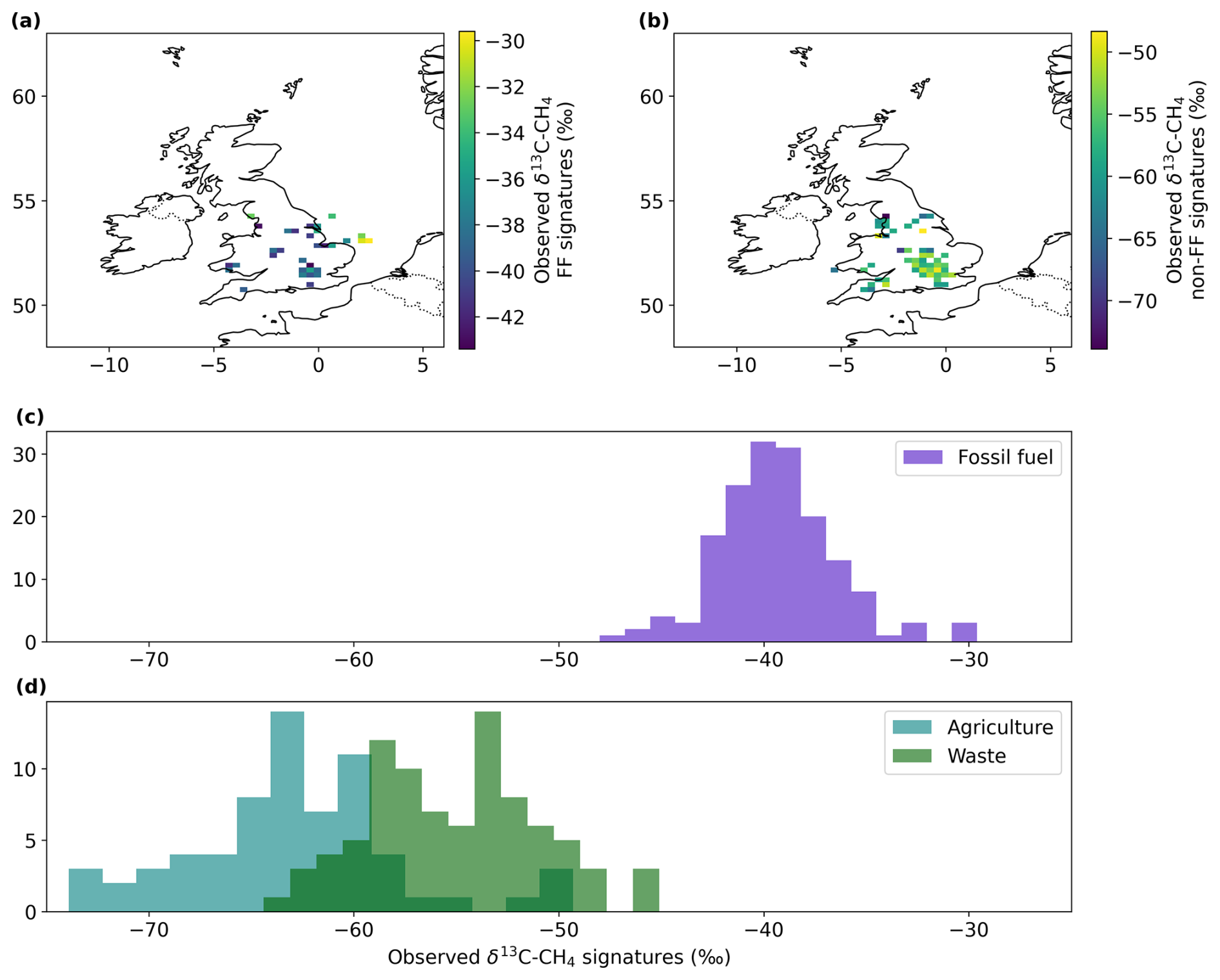
Figure B1 δ¹³C-CH₄ point source signatures compiled during the isoMET project (Dasgupta et al., 2025a, b) and observed by Royal Holloway during ground-based observation campaigns (Lowry et al., 2020; Menoud et al., 2022) from (a, c) FF and (b, d) non-FF sources. Point source signatures have been averaged spatially and temporally to the 25 km resolution of the atmospheric transport model used in this study. The same values are also presented as histograms, with non-FF sources split into (light blue) agriculture and (green) waste sources, showing the overlap between these two sectors.

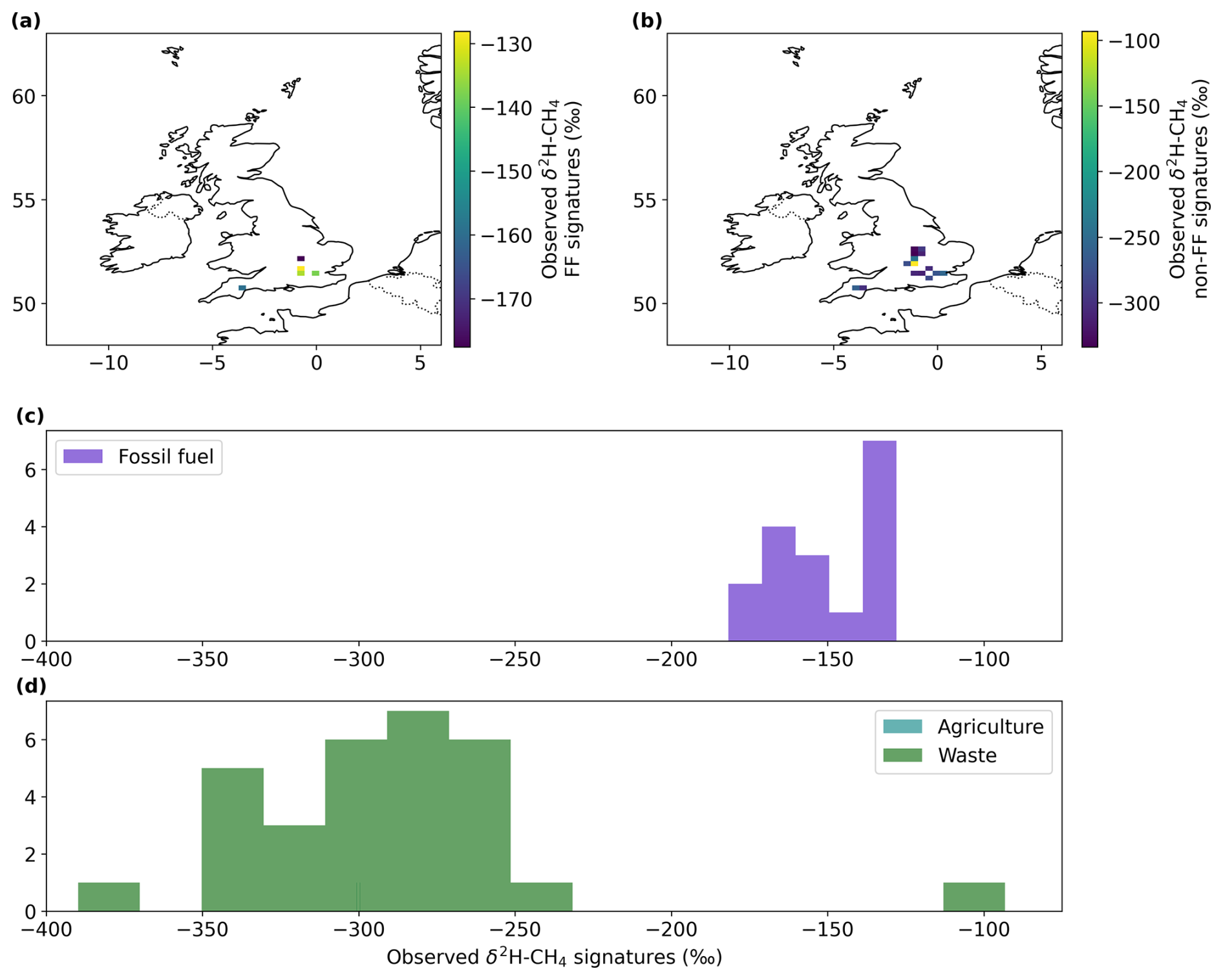
Figure B2 δ²H-CH₄ point source signatures compiled during the isoMET project (Dasgupta et al., 2025a, b) from (a, c) FF and (b, d) non-FF sources. Point source signatures have been averaged spatially and temporally to the 25 km resolution of the atmospheric transport model used in this study. The values are also presented as histograms. Only values for the waste sector are shown in the histogram, due to the lack of data for agriculture.

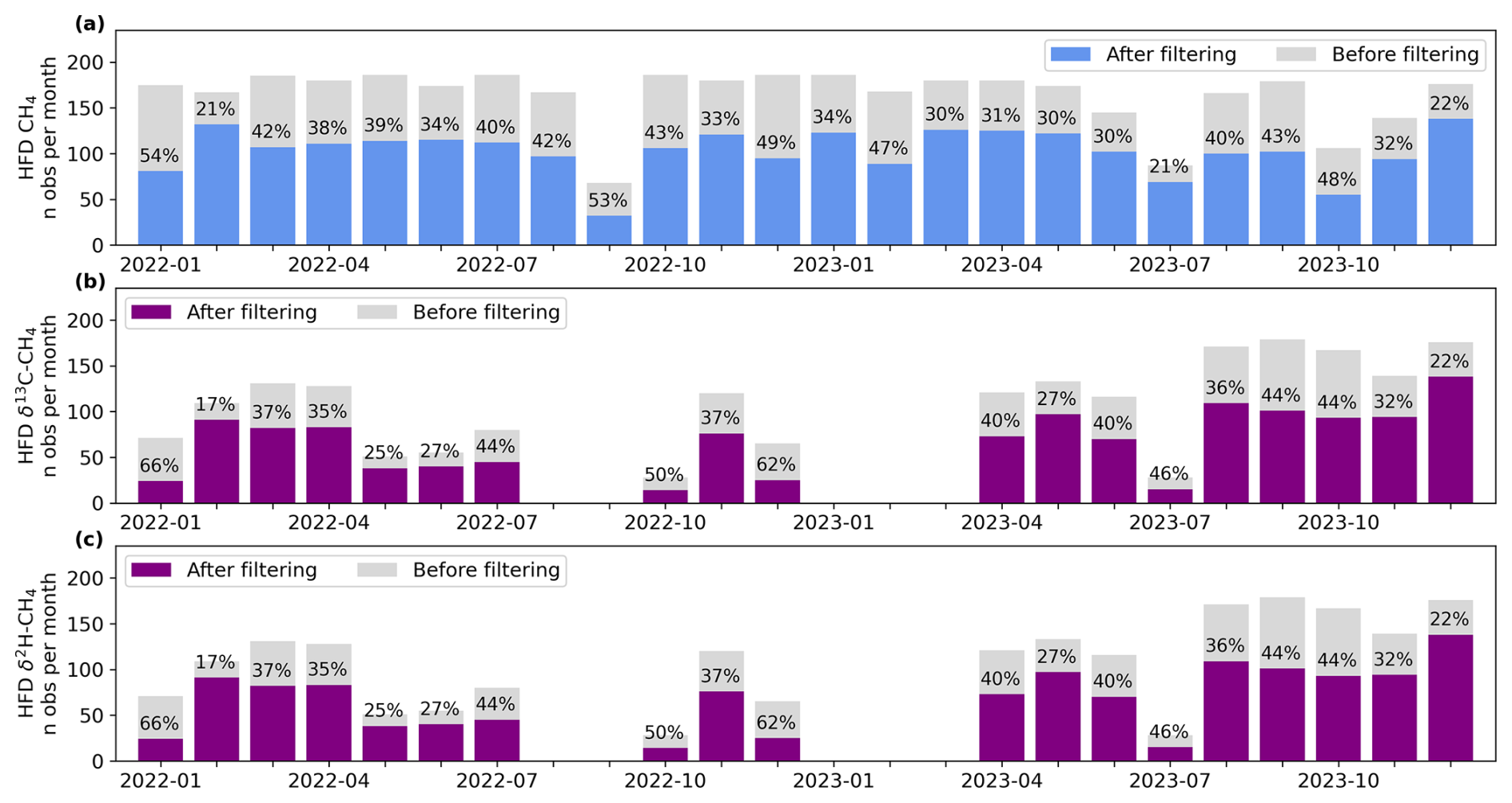
Figure B3 Number of 4-hourly averaged observations available from the Heathfield (HFD) site for each monthly inversion period before filtering (grey) and after filtering (coloured bar), for (a) methane, (b) δ¹³C-CH₄ and (c) δ²H-CH₄. Annotated values give the percentage of observations that were removed by filtering based on meteorological conditions (see Sect. 2.4.3 for more information on this filtering).

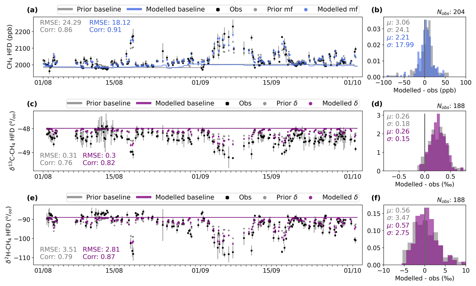
Figure B4 Modelled methane mole fractions and isotope ratios from Experiment 3r of the UK case study, with methane isotope ratio observations from the HFD site and fixed regional signatures. Four-hourly averaged observations (black squares) of (a) CH₄ mole fractions, (b) δ¹³C-CH₄ and (c) δ¹³C-CH₄ δ-values from the HFD site, for two example months August and September 2023. These are compared against (blue or purple) posterior modelled values and (grey) prior modelled values from the model with fixed source signatures. Differences between the observations and the (grey) prior and (blue or purple) posterior modelled mole fractions and δ-values are given on the right, as histograms. The mean and standard deviations of these model-observation differences are also given. (Grey line) prior and (blue or purple line) posterior mean baselines are also shown for comparison. For these model runs with fixed source signature terms, the prior and posterior baselines are identical for the isotope ratio terms.

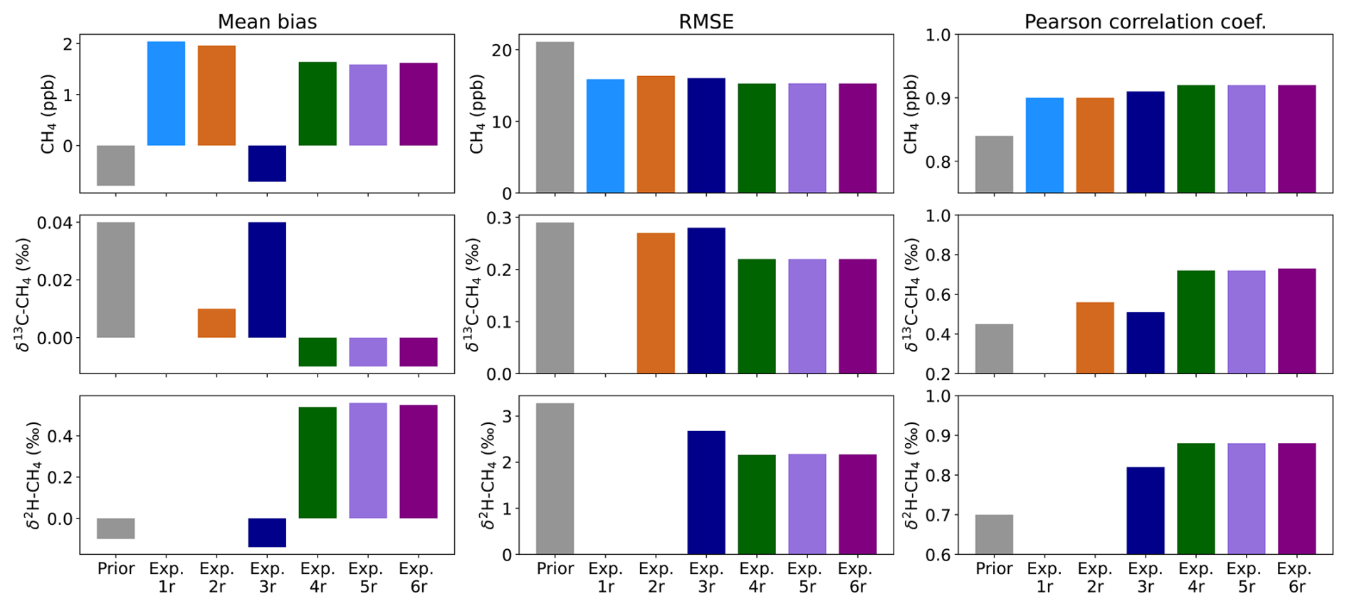
Figure B5 Statistics presenting the fit between observed and posterior mean modelled (top row) CH₄ mole fractions, (middle row) δ¹³C-CH₄ and (bottom row) δ²H-CH₄ for the six case study experiments (as described in Table 3). Statistics include: (left column) the bias between the posterior mean modelled and observed values, (middle column) the root mean square error (RMSE) between the posterior mean and observed values and (right column) the Pearson correlation coefficient of the posterior mean and observed values. The same statistics are given for the prior modelled mole fraction and isotope ratios, in grey.