Middle atmosphere chemical and dynamical effects in the CCMI-2022 stratospheric aerosol injection scenario

Stratospheric aerosol injection (SAI) could slow surface warming, however, potential side effects include changes in stratospheric ozone and changes in regional surface temperatures and precipitation resulting from tropical lower stratospheric warming. Previous multi-model studies have reported substantial discrepancies among models regarding these effects. Here we present results from the Chemistry-Climate Model Initiative Phase 2 (CCMI-2022), designed to constrain inter-model uncertainties by applying a common, transient stratospheric aerosol forcing to five chemistry-climate models that offsets surface warming after 2025 in a moderate greenhouse gas emission scenario. Simulations were analyzed between 2025–2099, and all models show a global total column ozone decrease in the first three decades of at most ∼ 10 DU relative to a no-SAI case. Tropical lower stratospheric heating differs by up to 4 K between models, but despite that, the models agree very well on the region of influence of key processes, like chlorine activation, nitrogen oxide passivation, and the strengthening of the deep branch Brewer-Dobson circulation. Therefore, the sign of the ozone anomalies due to SAI is consistent in all stratospheric regions except the lower polar stratosphere, although the contribution of different processes varies considerably. In three of the models, we separate pure chemical from dynamical (heating and nonlinear) contributions, and find that towards the end of the century, dynamical effects dominate ozone anomalies, except in the lower polar stratosphere, where heterogeneous chemistry plays a major role. Our findings highlight the need for sensitivity experiments on the absorptive heating and resulting dynamical effects under SAI.

1 Introduction

Human-made climate change is progressing faster than ever before (Allan et al., 2021; Pörtner et al., 2022; Forster et al., 2024). Global warming is likely to exceed the 1.5 K warming threshold set by the Paris agreement in the next years (Liu and Raftery, 2021), increasing the likelihood that some irreversible tipping points of the climate system will be triggered (McKay et al., 2022; Moeller et al., 2024). While the only permanent and sustainable solution is reaching net zero emissions, temporary amelioration of the surface warming could provide an opportunity to mitigate some of the adverse effects of climate change. Budyko (1977) and Crutzen (2006) proposed researching solar radiation modification (SRM) as a possible means of combating the rise in global surface temperatures. Stratospheric aerosol injection (SAI) is among the most discussed SRM concepts. The idea is to inject a sulfate aerosol precursor gas, which would artificially enhance the natural stratospheric aerosol layer – similar to a large explosive volcanic eruption. The resulting aerosol layer would scatter solar shortwave (SW) radiation, reflecting some of it back to space and thus producing a net cooling effect on the Earth system. Even if it were only possible to limit the rise in global mean surface temperature to 1.5 K relative to pre-industrial, rather than offsetting the entire anthropogenic effect, many of the impacts of climate change would likely be mitigated (Tollefson, 2018).

SAI carries potential side effects, some of which could be detrimental to the environment. Any perturbation to the natural stratospheric aerosol layer influences stratospheric temperatures, chemistry, and circulation (Robock, 2000; Marshall et al., 2022; World Meteorological Organization, 2022). Dynamical changes in the stratosphere can also propagate down into the troposphere, affecting regional surface climate beyond the intended global cooling effect (Hegerl and Solomon, 2009; Banerjee et al., 2021; Wunderlin et al., 2024; Tilmes et al., 2026). When considering SAI with sulfate aerosol particles, stratospheric temperature responds according to their radiative properties. Besides reflecting SW solar radiation, liquid sulfate droplets also absorb longwave (LW) radiation, largely from the Earth, effectively trapping terrestrial energy and heating up their surroundings. This absorptive heating is expected to lead to changes in regional precipitation and increase warming in the polar regions (Wunderlin et al., 2024). Likewise, altered meridional stratospheric temperature gradients after both volcanic eruptions and potential SAI deployment have been linked to changes in atmospheric dynamics (Marshall et al., 2022; Bednarz et al., 2023a). Another serious societal concern is ozone depletion, facilitated by heterogeneous reactions that occur on surfaces. These heterogeneous reactions are limited by the available surface area and the presence of ozone-depleting substances (ODS), therefore they are primarily important in the lower stratosphere (World Meteorological Organization, 2022). The ODS contain halogens, most notably chlorine and bromine, whose concentrations have been elevated through human activity for several decades. Even though the use of chlorofluorocarbons (CFC) and hydrochlorofluorocarbons (HCFC) has been strongly regulated, some emissions still remain (Western et al., 2023; An et al., 2025) and due to the long lifetimes of those compounds, concentrations will remain elevated in the stratosphere for decades (Bourguet et al., 2025). Because of the large ozone destruction potential that could be activated by SAI, several studies have focused on the extent of ozone loss caused by sulfur-based SAI (e.g., Pitari et al., 2014; Weisenstein et al., 2022).

Following Decision XXXI/2 of the Montreal Protocol on Substances that Deplete the Ozone Layer, which requested “information and research related to solar radiation management and its potential effect on the stratospheric ozone layer” (UNEP, 2019), the Chemistry Climate Model Initiative in its second phase (CCMI-2022) proposed a new model experiment, that simulates the effects of SAI between 2025 and 2100, by prescribing stratospheric aerosols properties, including surface area density and radiative properties, following an interactive SAI model simulation (Plummer et al., 2021; Tilmes et al., 2025).

To simulate a climate intervention scenario with stratospheric aerosol injection in its full complexity, a chemistry-climate model (CCM) with interactive aerosol microphysics is required. In recent years, the number of such CCMs has increased, enabling highly complex multi-model comparisons (e.g., Weisenstein et al., 2022; Visioni et al., 2023; Bednarz et al., 2023b). The sophistication of the different models is still variable, however, and these studies have shown that different aerosol modules can produce different aerosol burdens, surface area densities (SAD), and spatial distributions, leading to large uncertainties in the SAI effects (Pitari et al., 2014; Tilmes et al., 2021; Lee et al., 2026). Recently, Tilmes et al. (2026) showed that even within the same model, substantial differences in radiative efficiency and size-dependent sedimentation can arise when using a modal versus a sectional interactive aerosol scheme. The CCMI-2022 experiment circumvents such uncertainties arising from the representation of microphysical processes, by specifying a common stratospheric aerosol forcing in all participating models (Plummer et al., 2021), while also avoiding inter-model spread arising from differing equilibrium climate sensitivities (ECS), which necessitate different SAI injection amounts to achieve equivalent surface cooling. Here, we analyze the five models that contributed to this inter-comparison, describing the effects of SAI on the middle atmosphere, focusing on points of agreement and differences, and assess the remaining challenges.

2 Methods

2.1 Experimental setup

The CCMI-2022 scenario aims to identify the most important dynamic and/or chemical uncertainty factors in modeling the radiative and chemical effects of a prescribed artificially enhanced stratospheric aerosol layer. All models use the same prescribed aerosol layer in order to achieve a consistent forcing representation. Even models with interactive stratospheric sulfur cycle and microphysical module for the growth and development of sulfate aerosols replace this interaction with the prescribed aerosol. This study also does not aim to generate realistic SAI effects in the troposphere, as the sea surface temperatures are fixed as the climatological average of the years 2020-2029. We do not consider any tropospheric signals in this analysis.

The base experiment uses two model configurations: senD2-fix, a reference simulation with repeating 2025 aerosol climatology (replacing refD2 described below); and senD2-sai, an SAI simulation with a continuously increasing stratospheric aerosol burden. The difference between the two isolates the effects of SAI on the middle atmosphere. The resulting anomalies arise from chemical and dynamical changes that can also influence each other. The chemical impacts are directly driven by heterogeneous chemical reactions on the prescribed enhanced SAD, while the dynamics respond to the changes in radiative heating rates from both aerosol and chemical changes. The higher heating rates are a consequence of the increase in IR-absorbing stratospheric aerosol volume, and are in addition moderated by changes in ultraviolet (UV)-absorbing ozone. In the updated CCMI-2022 experiment presented here, we have added a third model simulation called senD2-chem, which simulates only the chemical effects of SAI, in order to better disentangle the separate roles of chemical and dynamical influences. The senD2-chem simulation is calculated by imposing only the changing SAD for the chemistry modules in the models, while all radiative properties of the aerosols are kept at 2025 conditions.

Table 1 summarizes the specified forcings for the three simulations senD2-fix, senD2-sai, and senD2-chem; transient greenhouse gas (GHG) forcings are adopted from the Shared Socioeconomic Pathway 2 (SSP2-4.5; “middle of the road” climate change scenario), while transient ozone-depleting substance (ODS) concentrations are taken from the 2018 report Scientific Assessment of Ozone Depletion (World Meteorological Organization, 2019). The more recent 2022 report was not yet available when some of these simulations were first started. The original description of the CCMI-2022 experiment is given in the Stratosphere-troposphere Processes And their Role in Climate (SPARC) Newsletter 57 (Plummer et al., 2021), 22–30 pp., with more additional description of the experimental setup and single-model results including comparisons to the interactive aerosol simulation are shown in Tilmes et al. (2025). The current study includes updates to the reference scenario and the additional simulation senD2-chem, which was not originally included in CCMI-2022. Subsequently, we document the protocol for these simulations in more detail.

World Meteorological Organization (2019)

Table 1 Specified forcings for the three simulations in the updated CCMI-2022 experiment. Adapted from Plummer et al. (2021).

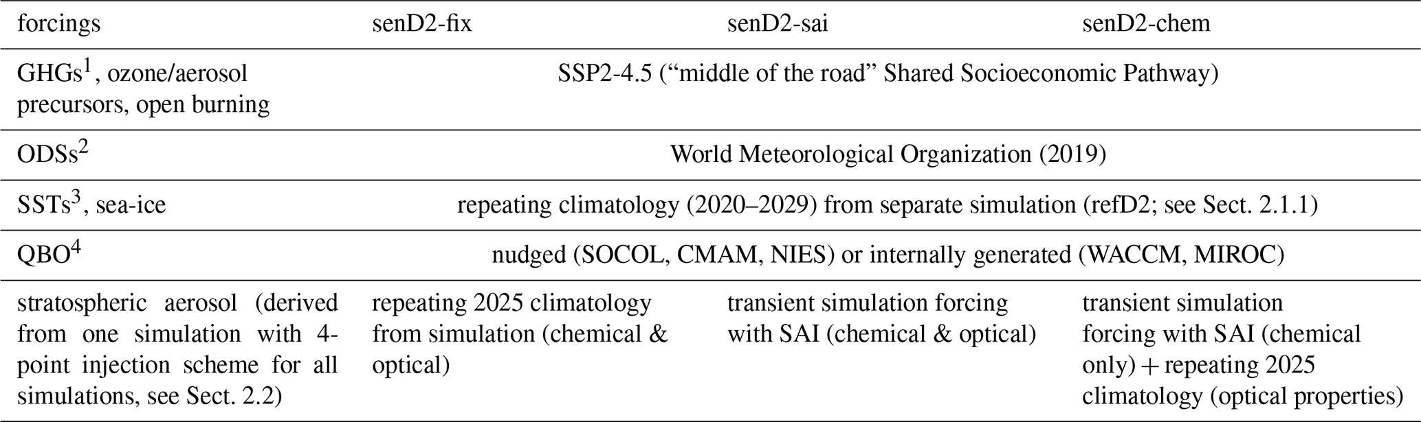
¹ greenhouse gases, ² ozone-depleting substances, ³ sea surface temperatures, ⁴ quasi-biennial oscillation.

2.1.1 refD2 (CCMI baseline future projection)

For the purposes of this analysis, the refD2 simulation can be regarded as a legacy case. We describe refD2 briefly, because some of its output is used as a forcing for the other simulations. refD2 consists of a historical and a scenario-driven part. It starts in 1960 and uses historical data on GHGs, ozone and aerosol precursors, and open burning data up to 2014 (Plummer et al., 2021). After that, these inputs follow the “middle of the road” climate change scenario SSP2-4.5 to the year 2100, with sea surface temperatures (SST) and sea-ice cover (SIC) calculated using a fully coupled ocean model; except for one model, where these boundary conditions are specified from another model with a coupled ocean (detailed in Sect. 2.3.3). The refD2 simulations are not used for analysis here, since senD2-fix with fixed SSTs and SIC provides a better reference for isolating the impact on the stratosphere. However, the 2020-2029 climatological SSTs and SIC from refD2 of each model served as input for the corresponding senD2-fix and senD2-sai simulations (see Table 1). A full description of refD2 with all its boundary conditions is given by Plummer et al. (2021).

2.1.2 senD2-fix (reference simulation)

For the senD2-fix simulation, we use repeating decadal mean SST and SIC climatologies from the respective refD2 simulations of each model and climatological stratospheric aerosol fields from the year 2025 of the prescribed aerosol data as fixed input over all years. The year 2025 represents a background state, because there is no SAI yet, however, the stratospheric aerosol layer is slightly enhanced to account for the average contribution of future volcanic eruptions (more detail in Tilmes et al., 2025). This background climatology has been derived separately and adapted to each model's individual radiation scheme (see Sect. 2.2). Other boundary conditions are identical to refD2 and can be found in Table 1. senD2-fix undergoes a five-year spin-up phase and begins its run on 1 January 2020 with SSP2-4.5 GHGs and World Meteorological Organization ODSs throughout the 21st century (Table 1). The senD2-fix simulation is not included in the original CCMI-2022 experiment description, but was designed to provide a more ideal reference simulation.

2.1.3 senD2-sai

The senD2-sai simulation is identical to senD2-fix with the exception of the stratospheric aerosol forcing. To simulate the effects of SAI, an enhanced and evolving aerosol layer above the tropopause is introduced into the models. This aerosol layer comes from a single model, namely CESM2 (WACCM6), and is uniformly prescribed in all models. The injection that creates this aerosol layer maintains the global mean surface temperature of the year 2025, which means that the injection rate increases over time. This means that for the first year (2025), the stratospheric aerosol forcing in senD2-fix and senD2-sai is identical, and thereafter the forcing in senD2-sai increasingly diverges from senD2-fix. A detailed description of the forcing, including its simulation, derivation, and processing, can be found in Sect. 2.2.

2.1.4 senD2-chem

In addition to senD2-fix, we introduce senD2-chem as an additional simulation to extend the analysis. To ensure comparability, there is only one difference between these simulations and the senD2-fix and senD2-sai simulations, namely the way in which stratospheric aerosols are implemented. The goal of senD2-chem is to separate the effects of SAI on stratospheric chemistry from its radiative effects. This is achieved by maintaining the radiative properties of the stratospheric aerosol at the 2025 levels of the forcing derived in WACCM (Sect. 2.2), whereas the full time-dependent surface area density for use in the stratospheric chemistry module is prescribed to be identical to senD2-sai. The senD2-chem simulation was only performed by three models: SOCOLv4, CMAM, and CCSRNIES-MIROC3.2 (see Sect. 2.3 for model descriptions).

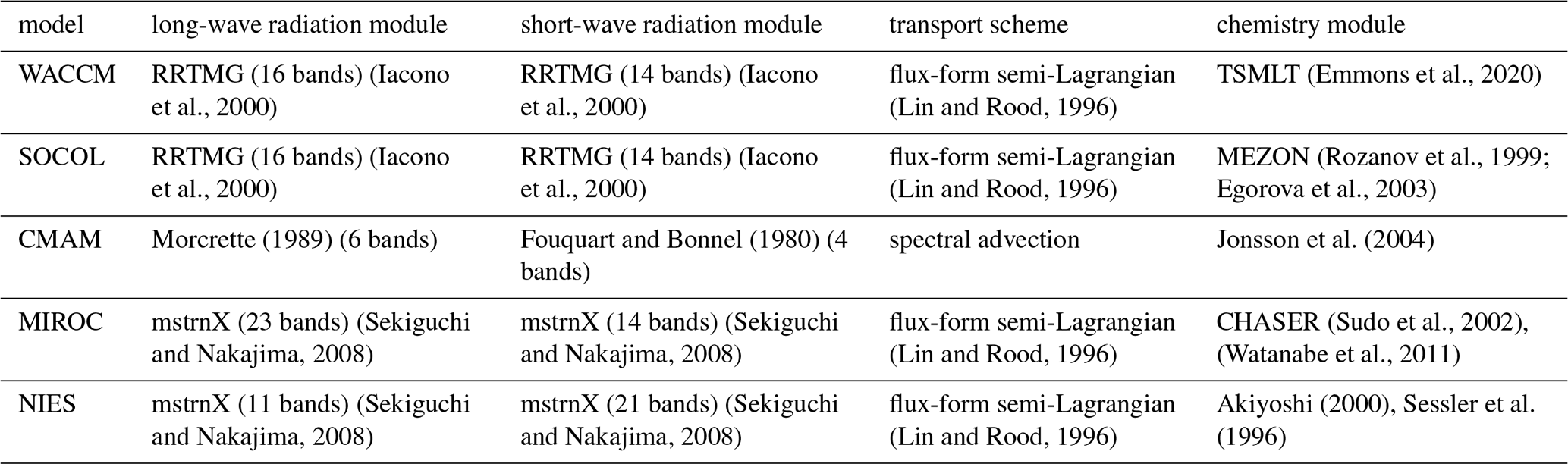
(Iacono et al., 2000)(Iacono et al., 2000)(Lin and Rood, 1996)(Emmons et al., 2020)(Iacono et al., 2000)(Iacono et al., 2000)(Lin and Rood, 1996)(Rozanov et al., 1999; Egorova et al., 2003)Morcrette (1989)Fouquart and Bonnel (1980)Jonsson et al. (2004)(Sekiguchi and Nakajima, 2008)(Sekiguchi and Nakajima, 2008)(Lin and Rood, 1996)(Sudo et al., 2002)(Watanabe et al., 2011)(Sekiguchi and Nakajima, 2008)(Sekiguchi and Nakajima, 2008)(Lin and Rood, 1996)Akiyoshi (2000)Sessler et al. (1996)

Table 2 Summary of the key modules for radiation, transport and (stratospheric) chemistry used in the prescribed version of each of the five chemistry-climate models in Sect. 2.3.

There is one complication, however, with the experimental setup that potentially introduces an inconsistency between some models. When the stratospheric aerosol is radiatively inactive, the photolysis rates do not take scattering of UV radiation on aerosol particles into account, which can impact photochemistry in the middle atmosphere. Neglecting the aerosol effect on photolysis in senD2-chem would therefore only isolate the “heterogeneous-chemistry” effect of the aerosol with respect to senD2-fix. However, the full chemistry effect, in principle, should also account for the photolysis effect, while keeping the radiative aerosol properties at background (2025) levels. This “full-chemistry” treatment is only possible in models that calculate photolysis rates online and thus can accommodate changes in photolysis due to the aerosol. In practice, the implementation is challenging and hence differs across the model ensemble. Therefore, out of the three models that performed senD2-chem simulations, two models (CMAM and SOCOLv4) do not adjust photolysis rates to the increasing aerosol load, while the other (CCSRNIES-MIROC3.2) does so. This means that in CMAM and SOCOLv4 the senD2-sai simulations also exclude the aerosol effect on photochemistry, potentially leading to a minor bias in the ozone tracer.

2.2 Stratospheric aerosol forcing

The aerosol layer applied in this work was generated similarly to the Stratospheric Aerosol Geoengineering Large Ensemble (GLENS) project documented by Tilmes et al. (2018). This utilized a feedback control algorithm (MacMartin et al., 2017) to adjust SO₂ emissions at four locations (15 and 30° N and S, 180° W; see Fig. 2 in Richter et al., 2018) in CESM1(WACCM) with the aim of maintaining global mean surface temperature (T₀), the inter-hemispheric temperature gradient (T₁), and the equator-to-pole temperature gradient (T₂) in a “high anthropogenic emission” scenario (RCP8.5). Different experiments were performed that injected at altitudes around 6 and 1 km about the tropical tropopause (Tilmes et al., 2021).

For the CCMI-2022 experiment, using the newer version CESM2-WACCM6 (see Sect. 2.3.1), the same four latitudinal locations for emission are chosen, with altitudes around 1 km above the tropopause (yellow squares in Fig. 1). In addition, the requirement of preserving the inter-hemispheric temperature gradient (T₁) is dropped, therefore the same injection amount is used for both Northern Hemisphere (NH) and Southern Hemisphere (SH) injections. This has been done to produce a more symmetric stratospheric aerosol distribution and aerosol optical depth in the two hemispheres, which facilitates multi-model comparisons (Tilmes et al., 2025). Further, in contrast to GLENS using RCP-8.5, CCMI-2022 employs the feedback-controlled SAI to maintain global mean surface temperature at 2020–2030 climatological levels in the “middle-of-the-road” scenario SSP2-4.5.

The stratospheric aerosol properties determined by CESM2-WACCM6 in the feedback-control run are then used as input to the other models. The input variables as function of latitude, altitude, and time are: (i) the SAD for the heterogeneous chemistry, and (ii) the optical aerosol properties for the radiative calculations, i.e. extinction coefficients, single scattering albedos, and asymmetry factors, each as function of wavelength. However, different chemistry-climate models have different treatments of the stratospheric aerosol in terms of different model grids (lat-alt) and different spectral wavelength bands in the radiative codes (Table 2). This makes it necessary to prepare the data individually for each model. Therefore, individual model forcings were derived from the original CESM2-WACCM6 stratospheric aerosol layer using the REtrieval Method for optical and physical Aerosol Properties in the stratosphere (REMAP) (Jörimann, 2025). The exact procedure for CCMI-2022, including the assumptions made to use size-related aerosol data from a modal aerosol model for Mie calculations, is detailed in Sect. 3.5 of Jörimann (2025). From the CESM2-WACCM6 data we produced the stratospheric aerosol forcing for each model on a zonal average latitude-altitude field ranging from 87.5° S to 87.5° N (in 5° steps) and from 0.5 to 39.5 km (in 0.5 km steps). The forcing provides monthly data from January 2020 to December 2100 (though we use the period 2025–2099 in this analysis). The data are archived in the ETH research collection (Jörimann, 2023).

Figure 1 shows the enhanced senD2-sai zonal mean stratospheric aerosol surface area densities averaged over two decades (2060–2079) for the boreal winter months December, January, February (DJF) and the boreal summer months June, July, August (JJA). This looks nearly identical across the five models, with small differences near the tropopause, whose height differs between models, as shown by the lines in Fig. 1. As only stratospheric SAD is prescribed, a stratosphere mask selects only values above the tropopause of each individual model, effectively truncating any non-zero grid cells below. In particular at higher latitudes the models cut out different parts of the forcing. Therefore, small inconsistencies in the modeled stratospheric aerosol (in the prescribed SAD and optical quantities) exist in the lowest levels of the stratosphere. However, the effect of the tropopause truncation on the latitude-weighted quantities is minor, as shown in Fig. 2a for the stratospheric SAD column.

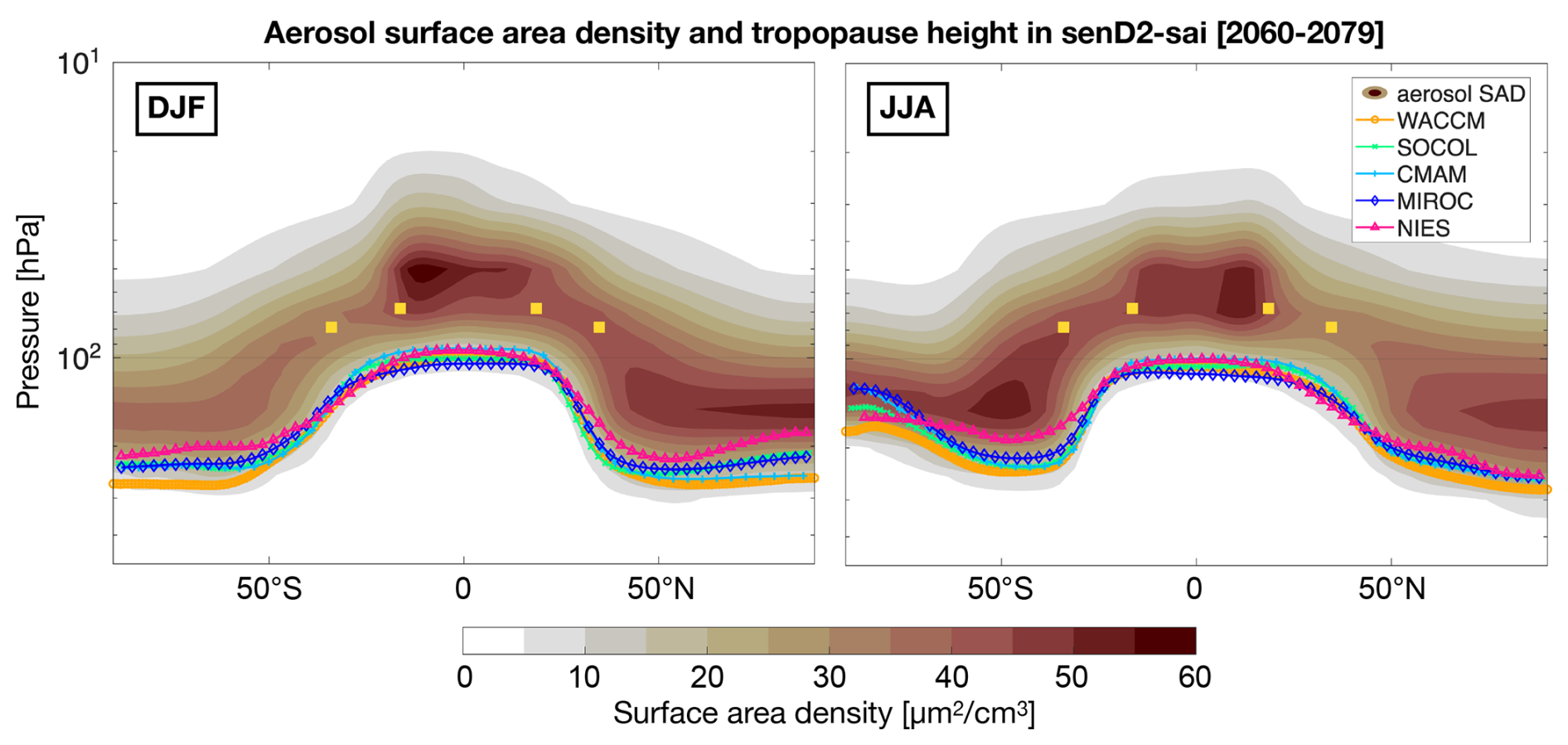
Figure 1 Artificially enhanced stratospheric aerosol zonal mean surface area density (SAD) output of a senD2-sai simulation (near-identical to prescribed SAD input). Contours: SAD from WACCM averaged over 20 years (2060–2079) for boreal winter (DJF, left) and summer months (JJA, right). Lines: Average tropopause pressure from all models (color-coded) over the same time period. Yellow squares: approximate positions of SO₂ emissions used to generate the depicted SAD.

2.3 Chemistry-Climate Models

We use chemistry-climate model data to assess the impacts of stratospheric aerosol injection on the middle atmosphere. The interplay of dynamical and chemical processes is vital for a good representation of nonlinear effects, notably affecting ozone production and destruction. This is congruent with the mission statement of the Chemistry-Climate Model Initiative (CCMI, 2022). To date, five models performed the CCMI-2022 experiment: CESM2-WACCM6, SOCOLv4, CMAM, MIROC-ES2H, and CCSRNIES-MIROC3.2. Versions of these models have all been used to produce realistic stratospheric ozone distributions and are well established in studies on ozone recovery (e.g. Dhomse et al., 2018; Friedel et al., 2023; Benito‐Barca et al., 2025). Each model's radiation modules, transport schemes, as well as chemistry modules are compiled in Table 2. The six heterogeneous chemical reactions on sulfate aerosol surfaces present in all five models comprise:

$$\begin{array}{rl}& {\mathrm{N}}_{\mathrm{2}}{\mathrm{O}}_{\mathrm{5}}+{\mathrm{H}}_{\mathrm{2}}\mathrm{O}\to \mathrm{2}{\mathrm{HNO}}_{\mathrm{3}}\\ & {\mathrm{ClONO}}_{\mathrm{2}}+{\mathrm{H}}_{\mathrm{2}}\mathrm{O}\to \mathrm{HOCl}+{\mathrm{HNO}}_{\mathrm{3}}\\ & {\mathrm{ClONO}}_{\mathrm{2}}+\mathrm{HCl}\to \mathrm{2}\mathrm{Cl}+{\mathrm{HNO}}_{\mathrm{3}}\\ & {\mathrm{BrONO}}_{\mathrm{2}}+{\mathrm{H}}_{\mathrm{2}}\mathrm{O}\to \mathrm{HOBr}+{\mathrm{HNO}}_{\mathrm{3}}\\ & \mathrm{HOCl}+\mathrm{HCl}\to \mathrm{2}\mathrm{Cl}+{\mathrm{H}}_{\mathrm{2}}\mathrm{O}\\ & \mathrm{HOBr}+\mathrm{HCl}\to \mathrm{BrCl}+{\mathrm{H}}_{\mathrm{2}}\mathrm{O}\end{array}$$

Two models (MIROC and NIES; see descriptions below) include more reactions on sulfate aerosol. For a complete list of reactions of all models, including heterogeneous reactions on nitric acid trihydrate (NAT) and ice aerosols, see Table D1. In the analysis, as well as in tables and figures we shorten the model names to “WACCM”, “SOCOL”, “CMAM”, “MIROC”, and “NIES”. We use ensembles with three members (realizations) for senD2-sai and one realization for senD2-fix and for senD2-chem per model.

2.3.1 CESM2-WACCM6 (“WACCM”)

The Whole Atmosphere Community Climate Model Version 6 (WACCM) is the atmospheric component of the Community Earth System Model Verion 2(CESM2) (Danabasoglu et al., 2020) and has a horizontal resolution of 0.95° × 1.25° and 70 vertical levels with a top at around 140 km. WACCM includes comprehensive chemistry in the troposphere, stratosphere, mesosphere, and lower thermosphere (TSMLT) (Gettelman et al., 2019; Emmons et al., 2020), including 231 solution species, 583 chemical reactions broken down into 150 photolysis reactions, 403 gas-phase reactions, 13 tropospheric, and 17 stratospheric heterogeneous reactions. The photolytic calculations are based on both inline chemical modules and a lookup table approach (Madronich and Flocke, 1998). WACCM includes a prognostic representation of tropospheric and stratospheric aerosols using Modal Aerosol Microphysics version 4 (MAM4) (Liu et al., 2016). The QBO is internally generated. The model is coupled to the Community Land Model version 5 (CLM5) (Lawrence et al., 2019). The configuration used here runs with a prescribed stratospheric aerosol distribution and prescribed SSTs and sea ice. WACCM ran the senD2-fix simulation until the end of 2083 (instead of 2099) due to resource limitations.

2.3.2 SOCOLv4 (“SOCOL”)

This is the ECHAM6-based version of the CCM SOlar Climate Ozone Links (SOCOL) of the Swiss Federal Institute of Technology Zürich (ETH Zurich) and Physical Meterorological Observatory Davos (PMOD, Sukhodolov et al., 2021). The dynamical core of SOCOLv4 is ECHAM6 (Stevens et al., 2013), which is interactively coupled to the chemistry module MEZON (Rozanov et al., 1999; Egorova et al., 2003), the Ocean Model of the Max Planck Institute for Meteorology Hamburg (MPIOM, Jungclaus et al., 2013), and the prognostic stratospheric aerosol microphysical model (AER Weisenstein et al., 2007; Sheng et al., 2015). It has a resolution of approximately 1.9° × 1.9° (T63), 47 vertical levels from the surface to 0.01 hPa, a dynamical time step of 7.5 min and 99 chemical species undergoing 304 reactions, including the major catalytic cycles of ozone destruction, as well as 16 heterogeneous reactions on surfaces of polar stratospheric clouds and aqueous sulfuric acid aerosols. Photolysis rates are calculated from a pre-computed look-up table and do not account for changes in aerosols. The QBO is nudged to the observed equatorial wind profiles. Different ensemble members were produced by changing the CO₂ concentration by ±0.5 %. For the purpose of the present work the ocean module MPIOM and the aerosol module AER are deactivated. Stratospheric chemistry in the prescribed model version has been tuned to decrease the bias in the total column ozone values with respect to the model version with an interactive aerosol scheme. This was done by halving the heterogeneous reaction rate coefficients on sulfuric acid aerosol surfaces. Potential reasons for the oversensitivity of halogen activation on prescribed aerosol surfaces might include the usage of monthly and zonal mean data, which can result in reaction rates under in-situ low temperatures to be too large.

2.3.3 CMAM

The Canadian Middle Atmosphere Model (CMAM) has been jointly developed by the University of Toronto, York University, and Environment and Climate Change Canada (ECCC). It is based on a vertically extended version of the 3rd generation Canadian Centre for Climate Modelling and Analysis (CCCma) Atmospheric General Circulation Model as described in Scinocca et al. (2008). The simulations used here were run at T47 spectral resolution (3.8° × 3.8° on the linear transform grid used for the calculation of physics) on 80 vertical levels up to the model lid at 0.0008 hPa. The atmospheric chemistry mechanism includes the HO_x, NO_x, ClO_x and BrO_x catalytic cycles that are important for controlling ozone in the stratosphere. Photolysis rates are calculated from a pre-computed look-up table and do not account for changes in aerosols in senD2-chem. The representation of polar stratospheric clouds includes supercooled ternary solution and ice polar stratospheric clouds (PSCs), which are calculated diagnostically based on local thermodynamic conditions. SSTs and sea-ice for the senD2-fix, senD2-sai, and senD2-chem simulations were taken from CCCma simulations submitted to CMIP6 using the 5th generation Canadian Earth System Model (CanESM5) (Swart et al., 2019).

2.3.4 MIROC-ES2H (“MIROC”)

The Model for Interdisciplinary Research on Climate – Earth System Model version 2H (MIROC-ES2H) was mainly developed by the Japan Agency for Marine-Earth Science and Technology (JAMSTEC) (Kawamiya et al., 2020). The present version of MIROC-ES2H is built on MIROC6 (Tatebe et al., 2019) and its atmospheric model has a spectral horizontal resolution of T85 (1.4° latitude × 1.4° longitude), which is loosely coupled with a lower horizontal resolution T42 (2.8° latitude × 2.8° longitude) chemistry climate model, Chemical Atmospheric General Circulation Model for Study of Atmospheric Environment and Radiative forcing (CHASER) (Sudo et al., 2002). These atmospheric models share 81 vertical levels from the surface to ∼ 0.004 hPa, with a vertical resolution of 0.7 km in the lower stratosphere, 1.2 km in the upper stratosphere, and 3 km in the lower mesosphere. The model spontaneously generates a QBO in the equatorial lower stratosphere. The configurations of atmospheric chemistry and aerosol modules are outlined in Watanabe et al. (2011). In the present simulations, the microphysics model for sulfate aerosols and volcanic ash (Sekiya et al., 2016) was deactivated in order to prescribe stratospheric aerosols. Photolysis rates are calculated online and capture the effect of UV scattering by an enhanced stratospheric aerosol. The three senD2-sai ensemble members have different initial conditions, which are based on the CMIP6 SSP2-4.5 ensemble simulations.

2.3.5 CCSRNIES-MIROC3.2 (“NIES”)

The CCSRNIES-MIROC3.2 CCM was constructed on version 3.2 of the MIROC3.2 atmospheric general circulation model (K1 Model Developers, 2004), incorporating the gas-phase stratospheric chemistry module that was developed at NIES (Akiyoshi, 2000) and heterogeneous reaction module developed by Sessler et al. (1996). The spatial resolution is a T42 spectral truncation (2.8° × 2.8°) in the horizontal direction, and the model has 34 vertical levels of hybrid sigma-pressure vertical coordinates from the surface to 0.01 hPa. The stratospheric chemistry module includes 42 photolysis reactions, 142 gas-phase chemical reactions and 13 heterogeneous reactions for sulfuric aerosols, supercooled ternary solution, nitric acid trihydrate and ice. Photolysis rates are calculated online and capture the effect of UV scattering by an enhanced stratospheric aerosol.

3 Results

3.1 Heating and Total Column Ozone Response

We start the analysis with the global mean stratospheric aerosol surface area density (SAD) integrated over all vertical levels above the tropopause to retrieve the average column loading shown in Fig. 2a. This serves to verify that the aerosol forcing remains consistent in the model output. By design, there is no temporal trend in senD2-fix while the stratospheric aerosol loading increases steadily in the senD2-sai simulation, with very good agreement between all models. The magnitude of the artificial aerosol forcing is comparable to the G6-1.5K-SAI experiment within the Geoengineering Model Intercomparison Project (GeoMIP Visioni et al., 2024), albeit slightly larger, because the temperature control starts earlier here. An anomalously strong annual cycle is present over the South Pole in CMAM (not shown), where the only output available is total SAD – as opposed to SAD from the sulfuric aerosol partition only. The surplus in CMAM thus comes from the addition of diagnostically calculated polar stratospheric clouds in the South Pole region and does not affect the analysis.

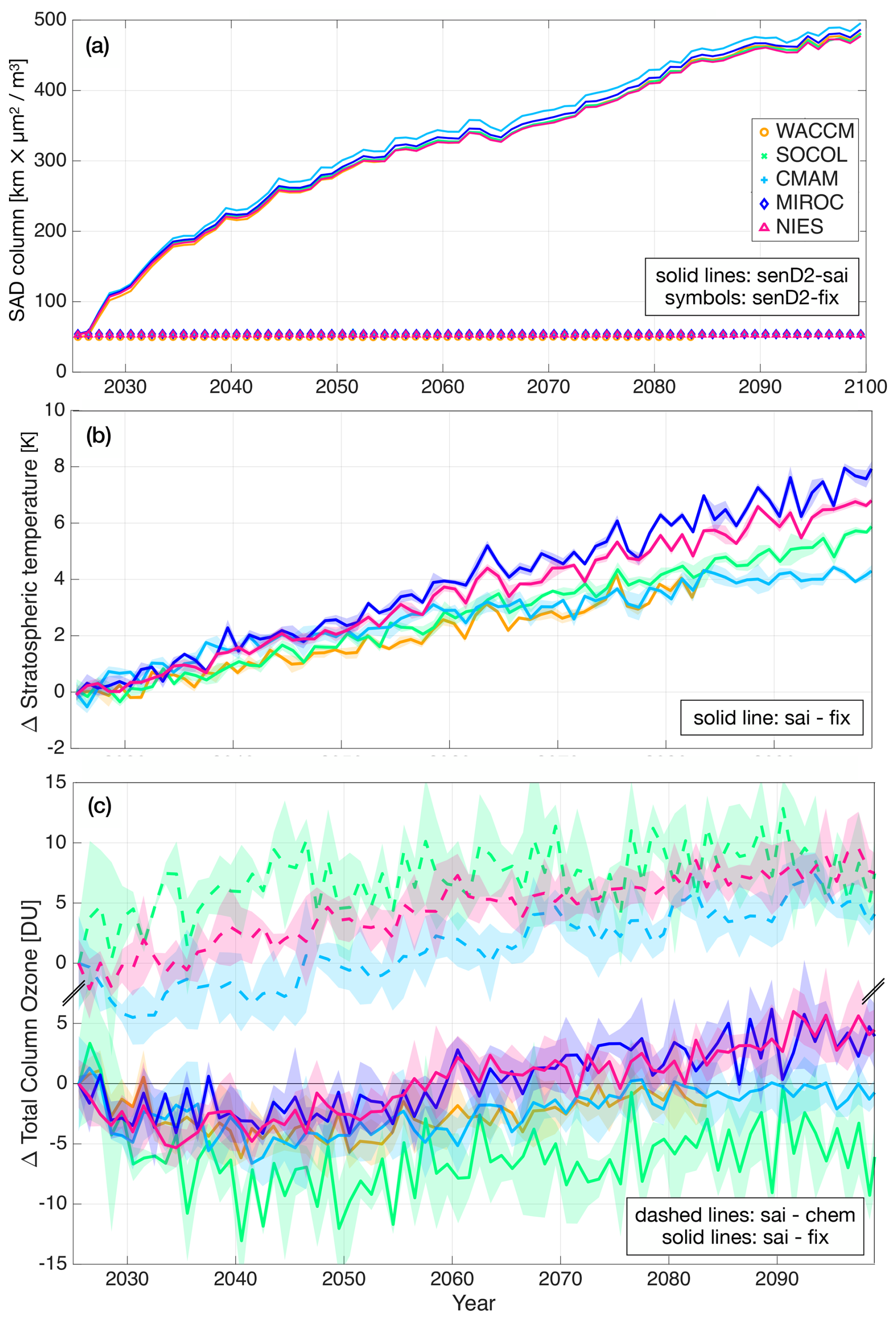
Figure 2 Stratospheric aerosol loading and resulting temperature and ozone changes for senD2-sai in the five models (color-coded). (a) Global and annually averaged column-integrated aerosol surface area density. Symbols: fixed aerosol forcing used in senD2-fix. Solid lines: aerosol forcing in senD2-sai required to maintain the original surface climate. (b) Stratospheric temperature anomaly due to SAI, senD2-sai – senD2-fix, averaged from 30° S to 30° N and from 115 to 70 hPa. (c) Global mean total ozone anomalies relative to 2025 due to full SAI (senD2-sai – senD2-fix; solid lines) and due to the dynamic signal alone (senD2-sai – senD2-chem; dashed lines). Data for WACCM senD2-fix is only available until 2083. Note the interrupted ordinate. Shaded areas in (b) and (c) confidence interval of one standard deviation.

Next, we discuss the effects of the simulated SAI on the lower tropical stratospheric temperature. The direct consequence of an increase in stratospheric sulfate is heating, as the droplets strongly absorb outgoing terrestrial radiation and, in addition, the much smaller amount of incoming solar infrared radiation. All models experience strong annual mean lower stratospheric heating, which is shown for the region between 115 and 70 hPa and 30° S and 30° N in Fig. 2b. The temperature increase varies between slightly more than 0.5 K per decade in WACCM and CMAM and about 1 K per decade in MIROC. Here, the models that include the same radiation scheme (WACCM and SOCOL: RRTMG; and MIROC and NIES: mstrnX) align closely in their temperature response, with WACCM and SOCOL showing about 1–2° less warming that MIROC and NIES by 2080. This indicates that differences in the radiation scheme may cause significant differences.

Figure 2c shows the SAI signal (defined as the difference in the SAI simulation compared to no SAI simulation over the same time) in global mean total column ozone (TCO) in all five models (solid lines) and the chemistry-only signal (dashed lines). All models indicate a decrease in global mean TCO during at least the first two decades compared to the respective no-SAI senD2-fix simulation. In the later part of the century, models disagree on the sign of the response, with MIROC and NIES showing a relative ozone increase due to SAI, WACCM and CMAM showing near-zero changes, and SOCOL continuing to show a negative ozone response throughout the length of the simulation. As mentioned in the SOCOL model description, prescribing sulfate aerosols in SOCOL resulted in its excessive chemical sensitivity to aerosol increase at coldest temperature locations, i.e. the lowermost stratosphere. This is further amplified in the polar areas due to feedbacks between chlorine activation, temperature, and vortex strength effects. Although SOCOL ozone anomalies outside of the lowermost stratosphere are in a good agreement with other models with no apparent biases (Fig. 3), this effect dominates the global mean TCO sign response for the given aerosol forcing. Regionally, this is the most apparent in the springtime South and North Pole TCO Fig. A1, where SOCOL shows the strongest ozone depletion. Note, however, that the Antarctic ozone depletion due to SAI was particularly strong also in the SOCOL G6 experiment with interactive aerosol microphysics, showing continuous TCO decline there even at the end of the 21st century (Wunderlin et al., 2024). In addition to causing changes in global mean total column ozone, the zonal distribution of TCO values will remain perturbed while SAI is active, as shown in Fig. A2. Models generally agree that the SH ozone response tends to be more negative by 2070–2083 than in the NH, where TCO is mostly positive. The positive TCO response in the NH is the strongest in MIROC and NIES, which contributes to their global mean TCO anomalies being the most positive and similarly distant with respect to CMAM as SOCOL, but with opposite sign Fig. 2c.

While the injection rate for generating the SAI scenario increases almost linearly with time (see Fig. 2b of Tilmes et al., 2025), the increase in the aerosol SAD column weakens over time. The stronger increase in SAD in the first 10–20 years is the result of increasing particle size with increasing injections (Tilmes et al., 2021). In contrast, stratospheric temperatures continue to rise unabated with continuously increasing mass. In the following sections we explore the response of the ozone distribution and the role of different processes.

3.2 Spatial ozone distribution changes

While annual and seasonal global TCO anomalies provide a view of the integrated ozone response, Fig. 3 provides a much more detailed view of the spatial anomalies in ozone mixing ratios (senD2-sai – senD2-fix; “full SAI”). The same figure but with ozone number concentration anomalies is provided in the Appendix (Fig. A3). As expected with a steadily increasing aerosol injection rate, the anomalies increase over time, and regional changes become statistically significant (t-test at 99  %). In all models the strongest signal occurs in the tropics, where a strong positive anomaly between 15 and 5 hPa is sandwiched between two negative anomalies centered at about 40 and 3 hPa. Directly above the tropical tropopause, some but not all models exhibit a small positive ozone anomaly. In the last of these 14-year averages, the middle stratospheric positive anomaly centered around 10 hPa and the negative anomaly above extend well into the mid-latitudes and all the way to the polar regions in some cases. The positive anomaly gets weaker farther away from the tropics, however, the negative upper stratospheric anomaly reaches a maximum at different extra-tropical latitudes – depending on the model. This meridional trend is only observed in the mixing ratio anomalies, though, due to the climatological ozone maximum in the tropics (see Fig. A3 for comparison). Finally, all models show significant ozone depletion over Antarctica (see also Fig. A1; more pronounced in Antarctic springtime, but clearly also visible in the annual average Fig. A2), whereas over the Arctic there are only weak negative TCO anomalies in the first few decades, which then become neutral and even consistently positive in CMAM, MIROC, and NIES in the second half of the century Fig. A2. Even for boreal springtime, Fig. A1 records no strong, lasting negative TCO anomalies in the Arctic after 2050, except for SOCOL, where strong ozone depletion of some 20–40 DU persists until the end of the century with no pronounced trend after the initial drop in the first 15 years, suggesting a balance between the competing effects of increasing SAI and decreasing CFC concentrations. Similar behavior is shown by WACCM in the Antarctic springtime (Fig. A1).

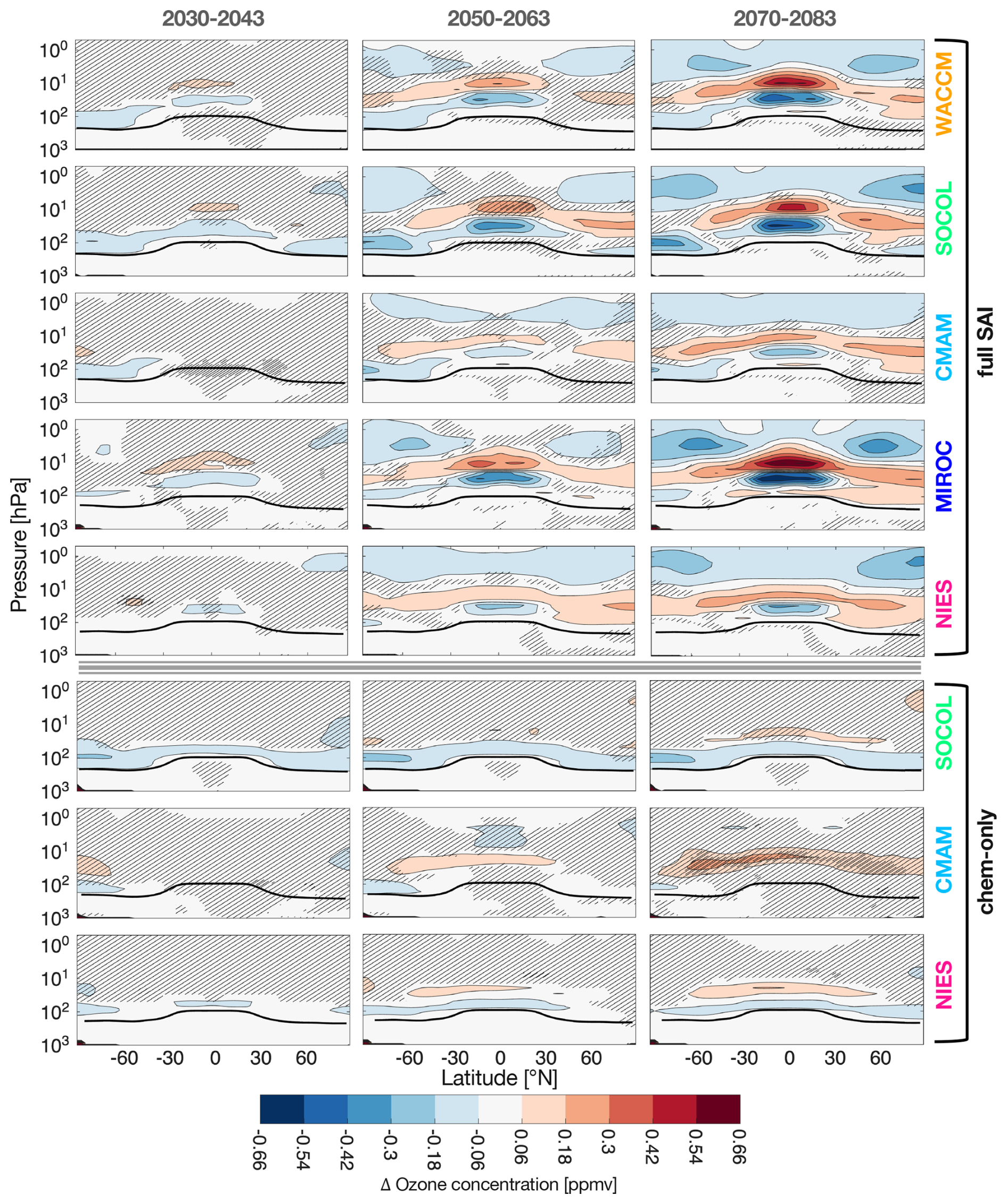
Figure 3 Zonal mean ozone mixing ratio anomalies in the full SAI scenario (senD2-sai – senD2-fix; top five rows) and for three of the models in the SAI chemistry-only scenario (senD2-chem – senD2-fix; bottom three rows). Anomalies are averaged over the 14-year time periods specified on top of each column. Black lines: mean senD2-sai tropopauses. Hatched areas: not significant at a 1 % level in a two-sample t-test.

The purely chemistry-driven signal – although differences in the implementation of photolysis exist – is diagnosed from senD2-chem – senD2-fix (“chem-only”, see Sect. 2.1.4). Its anomalies (bottom three rows of Fig. 3) are both simpler and of smaller magnitude than the full SAI signal, revealing the dominant role of the circulation in shaping the SAI impacts on the stratosphere. In the lower stratosphere, there is a negative ozone anomaly in two models, pole-to-pole in a layer about 5 km thick directly above the tropopause. Above the negative anomaly there are hints of a weaker positive ozone anomaly confined to the low and mid-latitudes. In CMAM the chem-only ozone mixing ratio signal remains statistically insignificant throughout the simulation, possibly because of high variability in the single senD2-chem realization. However, in the ozone number concentration anomalies in Fig. A3 the polar negative anomalies are more visibly pronounced, which shows a consensus between the models over chemical ozone depletion in the lower stratosphere over the South Pole.

3.3 Dynamical effects

When using sulfur-based aerosol particles for SAI at low latitudes, an unavoidable side effect is the aerosol-induced heating of the tropical lower stratosphere. This direct aerosol heating affects atmospheric circulation and transport of species, including ozone, and any changes in dynamics further feed back into and modulate the temperature response and rates of chemical reactions. We later attempt to disentangle these different processes with our additional senD2-chem experiment, but start the analysis of dynamical effects with the impacts of SAI (i.e. senD2-sai – senD2-fix).

The strongest temperature increase due to SAI is found in the tropical lower stratosphere and is roughly limited to 30° N and S. Despite strongly enhanced aerosol mass concentrations at the poles the models consistently produce a cooling over the Antarctic and in some cases over the Arctic as well. Due to limited insolation and relatively weak infrared emission from the surface, the absorptive properties of the particles are not the dominant control over temperature there. Instead, polar temperature changes are more strongly indicative of changes in dynamical heating (due to changes in downwelling and/or wave forcing), or changes in polar ozone itself. Positive extra-tropical zonal wind anomalies in Fig. 4 indicate a substantial strengthening of the westerlies that form the polar vortex (reported in Visioni et al., 2020; Tilmes et al., 2022), especially in the Southern Hemisphere. The polar vortex intensification – as previously mentioned – is most pronounced in SOCOL, which coincides with the largest cooling in the polar lower stratosphere and thus strongest increase in meridional temperature gradient out of all models. This polar lower stratospheric cooling can be attributed to the isolation of the polar air within the strengthened polar vortex, as well as enhanced polar ozone loss under increased SAD from SAI, both of which feed back into the zonal wind anomalies. There are indications of a weakening of the SH subtropical jet in a very confined region near the tropopause at 30° S from significant negative zonal wind anomalies, and in some cases in the NH as well. These are more pronounced in seasonal zonal wind anomalies (not shown here). For this experiment it can be expected that anomalies in the subtropical jets remain weaker than in some other SAI modeling experiments, because here the stratospheric aerosol is the only difference between senD2-sai and senD2-fix; the surface climate is similar in the two simulations. In studies that compare a surface warming scenario with an SAI scenario, larger anomalies due to differences in the wave breaking intensity that contributes to the subtropical jets are expected (cf. Fig. 2e in Wunderlin et al., 2024). Three of the five models included an idealized age of air tracer, and the resulting changes in mean age of air (in months) are shown in Fig. 4. All three models show positive anomalies in the tropical lower stratosphere in a narrow region near the tropopause, suggesting a slow-down of the shallow branch of the Brewer-Dobson circulation (BDC), and slowed tropical upwelling in the upper troposphere and lower stratosphere. Conversely, the air parcels in the entire middle and upper stratosphere up to the mesosphere experiences shorter residence times due to the aerosol heating-driven intensification of the deep branch of the BDC above the aerosol layer. The magnitude of this effect was found to be closely related to the magnitude of lower stratospheric heating within one model (Bednarz et al., 2023a) and here we see some indication of such a correlation existing also across the models here (with the largest heating rates observed in MIROC and the lowest in CMAM (see Fig. 2b). These substantial inter-model differences in zonal wind and age of air anomalies also suggest that the effect of an altered stratospheric aerosol burden on stratospheric dynamics, specifically transport barriers, may be majorly model-specific, which has previously been shown to be the case for the Mt. Pinatubo eruption (Perny et al., 2025). An additional signal that is only present in WACCM and MIROC, the two models that have an internally-generated QBO, is a potential modulation of the QBO (not investigated further here), as evidenced by changes in the zonal winds in the tropical middle stratosphere. A slow-down of the QBO or even a complete stall are potential effects with sulfur-based SAI that have been found under specific injection strategies with strong aerosol heating (Franke et al., 2021; Jones et al., 2022), however injections outside the equator minimize this effect (Richter et al., 2018).

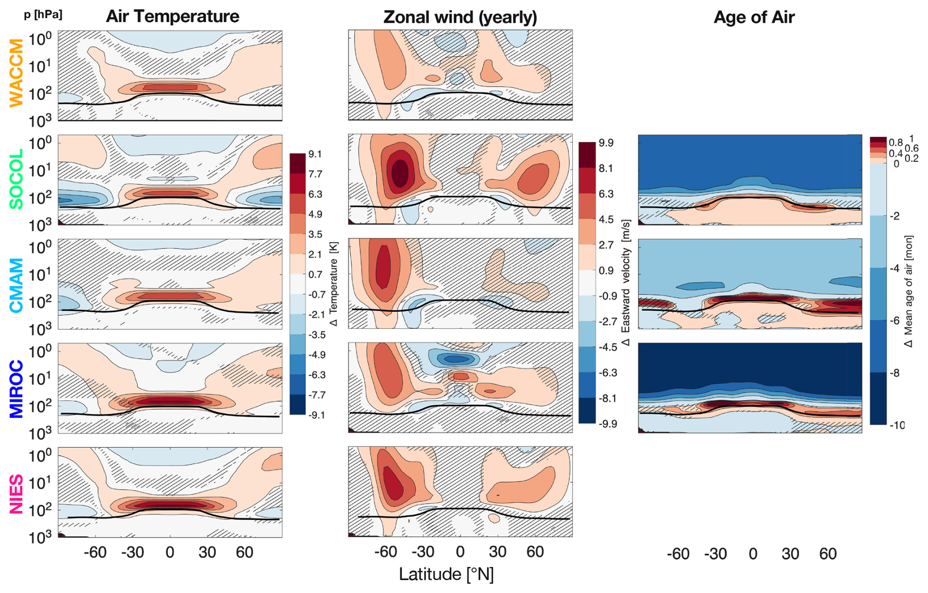
Figure 4 Zonal mean air temperature, zonal wind, and age of air anomalies due to SAI (senD2-sai – senD2-fix) for the 2060–2079 period. Black lines indicate the senD2-sai tropopause. Hatched areas are not significant at a 1 % level in a two-sample t-test.

3.4 Tropopause and cold point anomalies

Besides the strong effects on stratospheric circulation, the tropopause height and cold point temperature are both affected by SAI. The tropopause pressure anomalies (Fig. 5) are directly related to the temperature anomalies right above the tropopause. With strong heating the stratosphere effectively expands, lowering the tropopause height and thus resulting in positive tropopause pressure anomalies, simulated in all models in the tropics and well into the extra-tropics. In comparison to other SAI scenarios the tropopause pressure anomalies only arise from stratospheric heating – not from tropospheric cooling, which does not exist in this experimental setup (compare e.g. Fig. 3 in Lee et al., 2023). The inter-model differences are very well constrained in the tropics with the individual models diverging more and more towards the poles, even showing different directions in change over the Arctic. This reflects the level of ambiguity in temperature anomalies in those same regions well. Additionally to changing the altitudinal temperature profile, the aerosol heating raises the tropopause minimum temperatures, i.e. the tropopause cold point in the tropics. Fig. 5 shows minimum temperatures over 14-year time windows in an early and late window of the simulations. All models exhibit a warming trend in the tropopause cold point temperature in the senD2-sai simulation compared to senD2-fix. The warming across all models stays within 1 K for the first time window, then reaches a median between 2–4 K in the second window, where the scenario is more progressed. The tropopause cold point change has implications for the moistening of the stratosphere, as the tropopause acts as the bottleneck for water vapor to pass through into the stratosphere (see below).

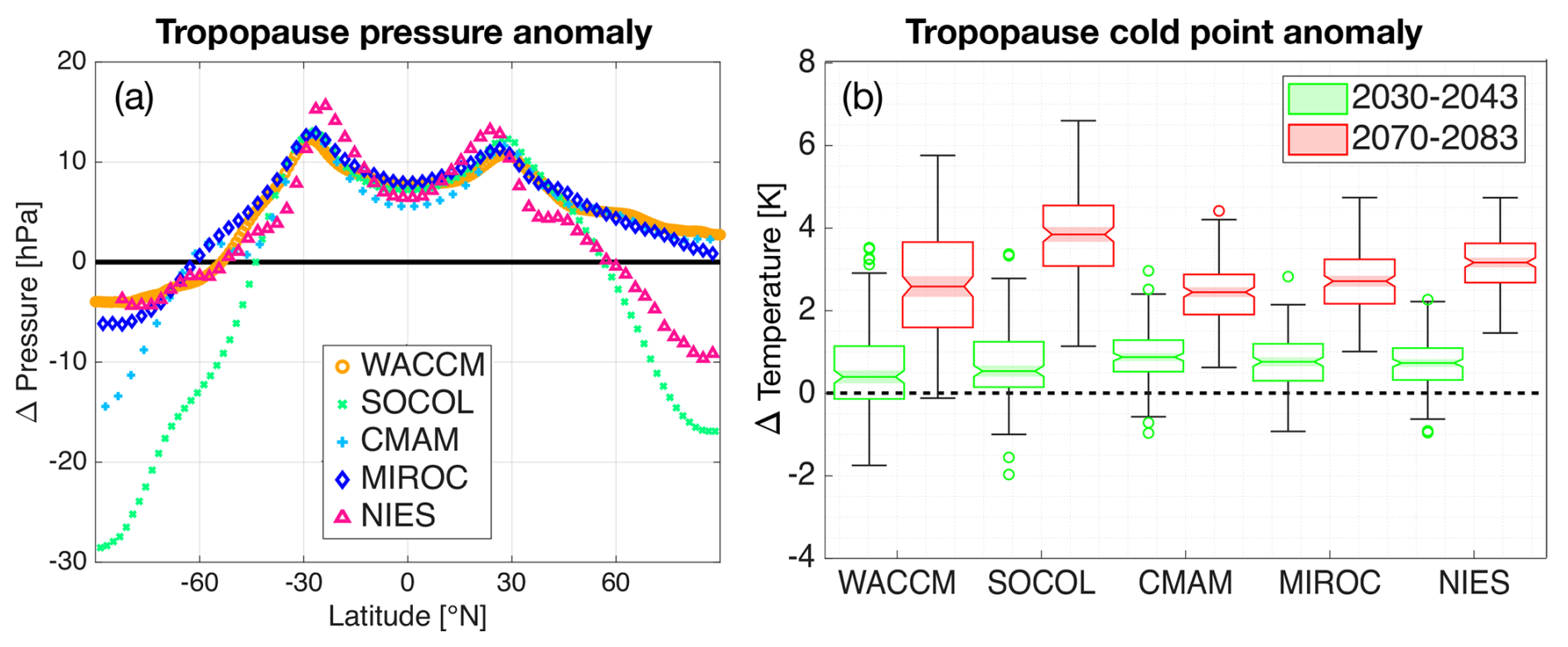
Figure 5 (a) Tropopause pressure anomaly as function of latitude caused by SAI (senD2-sai – senD2-fix) averaged over 2070–2083. (b) Anomaly in tropopause cold point temperature between 30° S and 30° N due to early-stage (green) and advanced (red) SAI (senD2-sai – senD2-fix). Whisker plot shows the spread of monthly mean data (minimum, first quartile, median, third quartile, maximum, and outliers.

3.5 Effects of aerosol heating on key chemical species

With the changes to the temperature profile come important changes in the concentration of a number of chemical species. Figure 6 shows water vapor (H₂O), methane (CH₄), and nitrous oxide (N₂O) mixing ratio percentage anomalies as a result of SAI. These species are all greenhouse gases and they can be a source of active agents participating in ozone depletion. All the anomalies above the tropopause in this figure are positive as a result of temperature and circulation changes. The strongest percentage increase in H₂O is found just above the tropical tropopause layer (TTL) in SOCOL, which features the largest tropopause cold point warming, freezing out less water and allowing air with a higher humidity to pass into the stratosphere. The percentage (as well as absolute) anomalies assume their highest values just above the TTL in all models and decrease with height and towards the poles. As a result the signal is less stratified than for CH₄ and N₂O, indicating a shorter lifetime due to the reaction with excited, monatomic oxygen O(¹D) to form hydroxyl radical (OH). The strongest increase in CH₄ and N₂O is recorded in MIROC, which produced the highest heating rates and the largest increase in tropical upwelling. The other models show more modest positive anomalies, with CMAM even lacking a significant widespread signal in CH₄ anomalies. The strength of the CH₄ and N₂O anomalies is very well anti-correlated with that of the age of air anomalies in the three models that provide them Fig. 2, but this is not the case for H₂O, which confirms that an additional process acts on H₂O, while the other two species are more tracer-like. The CH₄ and N₂O anomalies are largely stratified and increase with greater height, because these two gases are relatively long-lived and thus able to reach the upper stratosphere, where their concentrations in senD2-sai increase due to the stronger circulation. In the absolute CH₄ and N₂O anomalies there are maxima between 10 and 1 hPa (not shown here), while the percentage anomalies continue increasing with height due to smaller and smaller background concentrations. Figure 6 demonstrates that the TTL temperature and circulation changes in the middle atmosphere exert meaningful control on the abundance and distribution of chemical species that play a role as source gases of ozone-depleting agents that we will consider next.

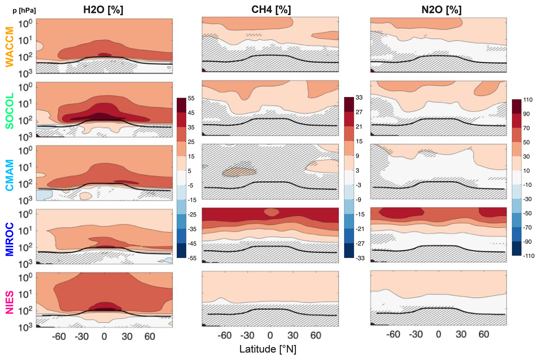
Figure 6 Relative zonal mean anomalies (in %) of water vapor, methane, and nitrous oxide mixing ratio caused by SAI (senD2-sai – senD2-fix) for the period 2060–2079. Black lines: senD2-sai tropopause. Hatched areas: not significant at a 1 % level in a two-sample t-test.

3.6 Partitioning of ozone-depleting agents in active and passive compounds

Chemistry in the middle atmosphere is characterized by chemical families that produce or destroy ozone in catalytic cycles and interact with each other by forming reservoir compounds. Changes to those interactions and changes to the concentrations of involved species result in new dynamic equilibria and a new ratio of active (i.e. capable of participating in ozone-depleting reactions) and passive (reservoir) species. The three major chemical families that are affected by sulfur-based SAI are the nitrogen oxide (NO_x), odd hydrogen (HO_x) and chlorine oxide (ClO_x) families. We assume bromine oxides (BrO_x) play a minor role and do not include them in the analysis, although some bromine family reactions are included in the models. For NO_x the models are in qualitative agreement over a bipolar structure with negative anomalies in the lower and middle stratosphere – i.e. in the region where NO_x-catalyzed ozone depletion is most important – and positive anomalies above 10–5 hPa. In fact, the reversal from negative to positive signal is in very good agreement across the models, which is reflected in Fig. 9a, where only a small hatched region in the tropics around 5 hPa indicates that not all models agree on the sign of ozone change. The main disagreement comes from CMAM, which has the strongest NO_x loss that extends up slightly higher than the other models. The negative anomaly can be explained by the SAI-induced acceleration of N₂O₅ hydrolysis on aerosol surfaces that consumes NO_x and is further facilitated by enhanced water vapor availability. The positive anomaly higher up can be attributed to the dynamically-induced N₂O increases, which is a source gas for NO_x. Even better agreement is shown in the HO_x response to SAI, where all models show the same spatial structure stay within a factor of 1.5 of each other in absolute concentration change (see Fig. B1). The positive HO_x anomaly stems from the water vapor increase. The ClO_x trends are more complex, since the heterogeneous chemistry of this family is more sensitive to temperature. With aerosol surface area density levels many times that of the background state, chlorine activation on aerosol surfaces is expected to intensify in all places, where the aerosol intersects the regions that reach low enough temperatures. Anthropogenic chlorinated compounds (e.g. CFCs) are still in the atmosphere after 2060, albeit at lower levels than in present day. Therefore, the models agree that SAI promotes the available chlorine to be converted into active species (ClO_x) in the lower stratosphere. The main hotspots for chlorine activation are the poles, where winter and spring conditions enable heterogeneous chlorine activation reaction chains, and in some cases the tropical tropopause. The degree of chlorine repartitioning into active species is particularly sensitive to the model, as demonstrated in the differences in magnitude of the anomalies in Fig. 7. In the upper half of the stratosphere there is also no clear consensus between the models with significant negative anomalies in only two models. We note here that absolute anomalies do not take into account the background state of each model, which may already contain different climatologies. We include percentage anomalies of the same species in the Appendix (Fig. B1), which are especially highly variable in ClO_x, but also show substantial variance across models for HO_x and NO_x. Fig. B1 shows that the upper stratospheric ClO_x percentage anomaly is very small compared to the lower stratosphere. Since CFC concentrations and aerosol SAD are both prescribed in this experiment, differences in chlorine activation can only come from the model-specific treatment of heterogeneous reaction or ambient conditions (e.g. temperature). We provide a comprehensive table of heterogeneous reactions and which surfaces they are active on in each model in Table D1, which indeed shows that apart from the six main reactions on sulfate aerosols that all models include (listed in Sect. 2.3), only some models include more heterogeneous reactions. While these additional reactions may be able to explain, why NIES shows the strongest tropical lower stratospheric chlorine activation, it fails to explain why MIROC, with the same reactions as NIES, shows lower chlorine mixing ratio anomalies overall, even being close to zero in the tropical lower stratosphere despite MIROC having a lower tropopause cold point temperature than NIES (Fig. 5b). The number of reactions included also does not generally correlate with the intensity of chlorine activation in the other models. Therefore, it is more likely that differences in the implementation of heterogeneous reactions (e.g. reaction rates), or differences in ambient conditions are the cause of this variability.

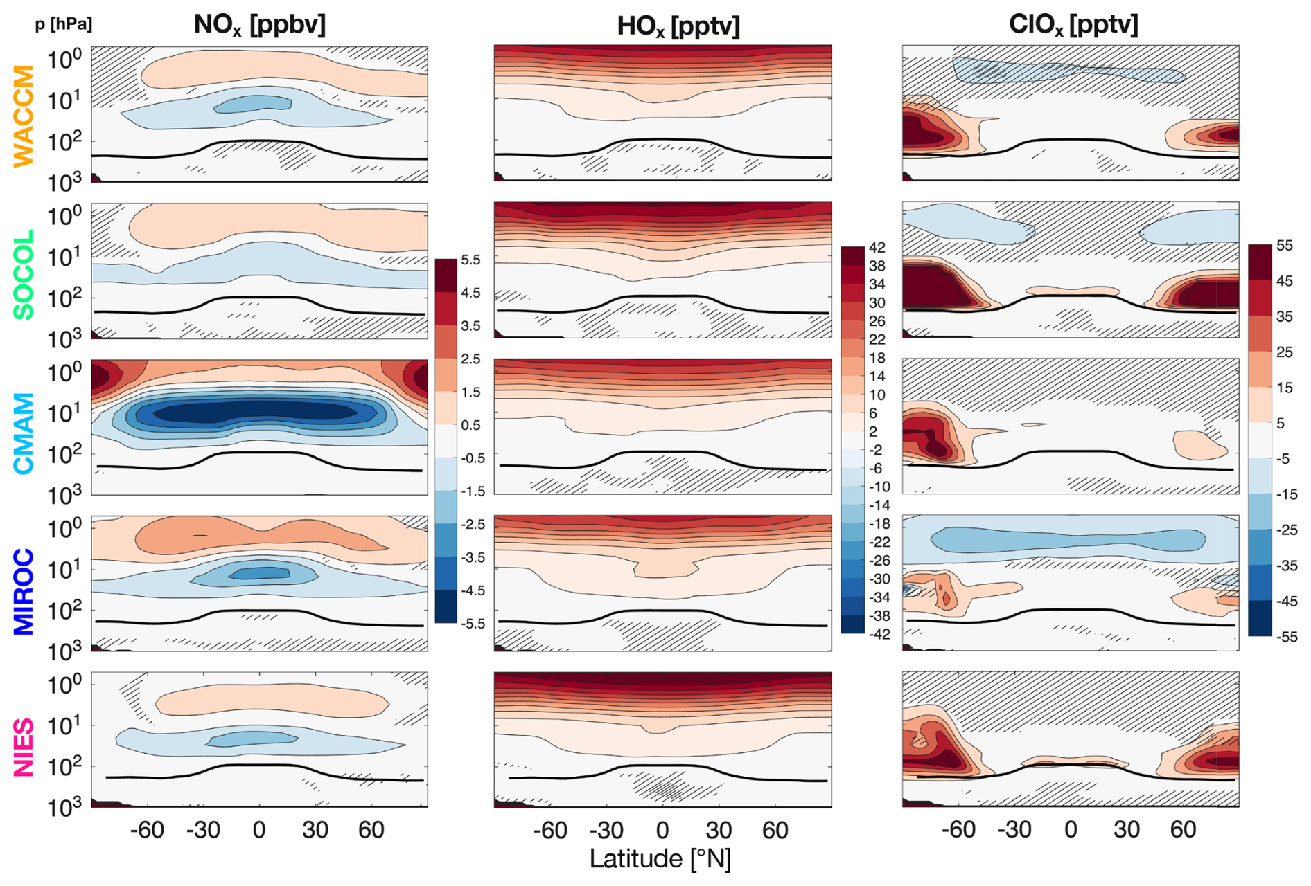
Figure 7 Zonal mean mixing ratio anomalies of active nitrogen oxide (NO + NO₂ + 2 × N₂O₅), active hydrogen oxide (OH + HO₂), and active chlorine (oxide) (Cl + ClO + 2 × Cl₂O₂) caused by to SAI (senD2-sai – senD2-fix) for the period 2060–2079. Black lines: senD2-sai tropopause. Hatched areas: not significant at a 1 % level in a two-sample t-test.

To better understand the activation/deactivation effect of SAI we also provide the anomalies of some important reservoir gases that represent the passive partition. Given the right conditions, ClO_x and NO_x can be converted into hydrochloric acid (HCl), chlorine nitrate (ClONO₂), and nitric acid (HNO₃) – or, in reverse, the reservoir gases can be activated. We show mixing ratio anomalies of these three reservoir gases due to SAI in Fig. 8. In the lower and middle tropical stratosphere there is a strong dynamical control on all reservoir gases, which creates a similar dipole structure of positive anomalies around and just above the tropopause and negative anomalies between some 70 and 30 hPa. The increase in the lower stratosphere is especially well recorded in the percentage anomalies of the reservoir gases (supplied in Fig. B2) and comes from the slowed shallow branch of the BDC, which draws tropospheric air up into that region less quickly and exports it out of that region less efficiently than without SAI (cf. Fig. 4). This causes a relative increase in concentrations, as tropospheric air has lower concentrations of all three reservoir gases, and the effect is mainly limited to the tropics, with some leakage into the mid-latitudes. The negative tropical anomalies above partly stem from the strengthened deep branch. This pattern is only broken in the HCl anomalies of SOCOL and NIES, which are entirely negative in the tropical lower and middle stratosphere. This comes from the chemical conversion of HCl into ClO_x on sulfate aerosol particles, as evidenced by the ClO_x enhancement there in the same two models (Fig. 7). Heterogeneous chemical chlorine activation also leads to negative HCl anomalies across models from some kilometers up from the tropopause into the middle stratosphere in the extratropics. Further up, in the middle stratosphere and towards the mesosphere, HCl does not show significant anomalies, because temperatures are high enough to evaporate any aerosol that may be transported up from below, leaving no surface area for heterogeneous chlorine activation to take place on. Chlorine nitrate mostly lacks significant anomalies that are consistent across the models, suggesting a complex change in the new chemical equilibrium due to multiple processes – or, possibly, differences in the heterogeneous chemical reactions that are included in each model and influence ClONO₂. In HNO₃ some negative anomalies exist in the lower southern polar stratosphere (and sparsely in the North, although models disagree) and extend into the troposphere and are likely the result of denitrification. Apart from these regions and the dynamical negative anomaly in the tropics, however, HNO₃ anomalies are widely positive with a peak around 20–30 hPa, due to N₂O₅ hydrolysis (correlating with NO_x depletion).

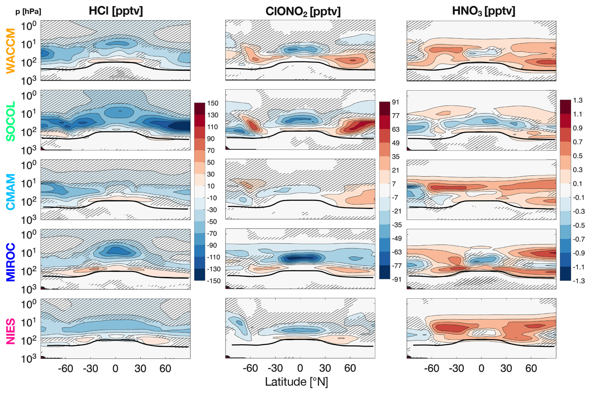
Figure 8 Zonal mean mixing ratio anomalies of hydrochloric acid, chlorine nitrate, and nitric acid mixing ratio [(senD2-sai – senD2-fix)/senD2-fix] caused by SAI for the period 2060–2079. Black lines: senD2-sai tropopause. Hatched areas: not significant at a 1 % level in a two-sample t-test.

3.7 Multi-model mean and key regions

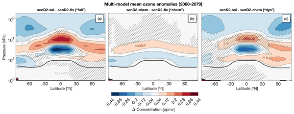
In this section we synthesize the key findings from across all models and point out the inter-model agreements and differences. Figure 9 shows the ozone anomalies averaged over all five participating models for the same time period (2060–2079, inclusive) used before. We show the anomalies in ozone concentration due to SAI (“full”) in panel (a). Panel (b) shows the anomalies from only the chemical effects of SAI (“chem”) and panel (c) shows the difference between “full” and “chem”, which equates to the linearly isolated dynamical effects (“dyn”) of SAI. This does not represent a clean isolation of dynamical effects, but rather an approximation, where nonlinearities and differences in treatment of photolysis due to aerosol UV scattering in senD2-chem are still included. Since panels (b) and (c) require the senD2-chem simulation, they only include the three models for which these simulations are available: SOCOL, CMAM, NIES. The “full” anomaly for these three models only – with respect to which “dyn” is derived – is given in Fig. C1. Shading in the entire figure indicates that at least one of the models disagrees about the sign of the anomaly. We define some key regions in the latitude-vertical domain of the panels to distinguish between different dominant processes. We give a short summary for each of these regions to describe the multi-model ozone anomalies:

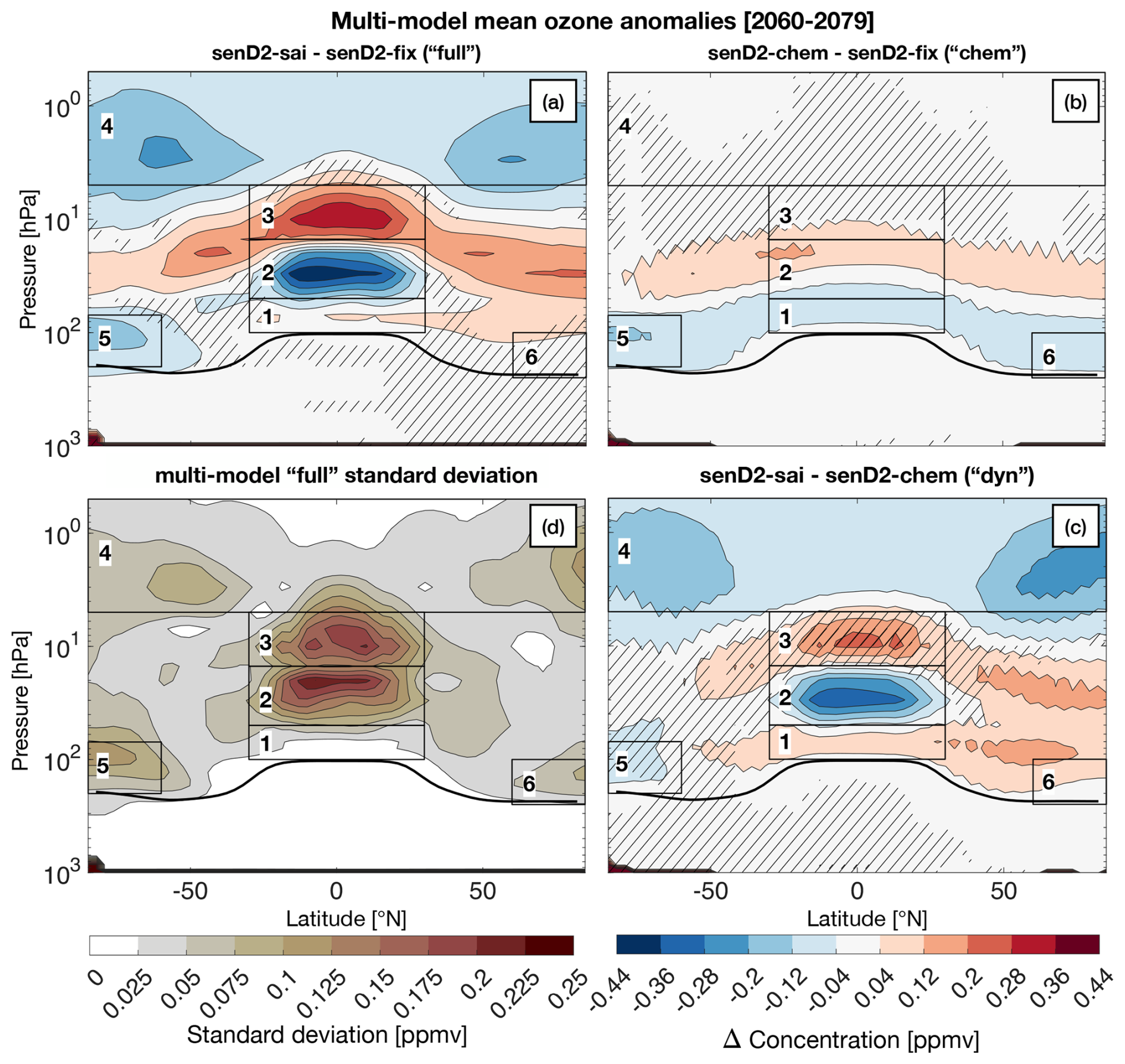
Figure 9 Multi-model mean zonal mean ozone mixing ratio anomalies due to full SAI (senD2-sai – senD2-fix; panel a), the standard deviation of full SAI in panel (d), only chemical effects of SAI (“chem”; panel b), isolated dynamical effects (“dyn”; panel c). Panel (a) is the multi-model mean of all five models, panels (b) and (c) show multi-model means of the three models that simulated the senD2-chem simulation. The “full” model mean of the same models that were used in panels (b) and (c) is not shown here, but added in Fig. C1. The standard deviation in panel (d) pertains to panel (a). The black rectangles show regions with a dominant process shaping the ozone anomaly signal. The black line indicates the tropopause. Regions where the sign of all models do not agree are hatched.

1. In the tropical lowermost stratosphere the SAI effect on ozone is smallest out of the chosen regions, because the negative chemical effect and the positive dynamical effect almost cancel each other out. While the deep BDC branch increases, the shallow branch is weakened (see Sect. 3.3). This leads to less transport of ozone-poor air from the troposphere to the tropical lower stratosphere, less efficient export to mid-latitudes and thus an increase in ozone concentration. This effect is partly counteracted by tropical chlorine activation, which is apparent in “chem”, but the anomaly is still consistently positive across all models (see also the ozone number concentration anomaly in Fig. A3).

2. In the tropical lower stratosphere the models agree well in “full”, “chem”, and “dyn”. The strong negative anomaly in “full” can be attributed almost entirely to dynamics. The chemical contribution in region 2 changes from negative (bottom) to positive (top) in this region, but is weak overall. The dynamical signal arises from the strong aerosol absorption heating, which increasingly draws comparatively ozone-poor air up from below. The largest variability here is observed towards the top of the box, which indicates that the negative anomaly varies one or two model levels in extent between the models and the reversal to positive comes earlier (lower down) in some than in others.

3. Region 3 receives its positive anomaly in all models from the increased BDC deep branch strength, like region 2. Air comparatively rich in ozone from the main formation region below is transported faster in the tropical pipe and brings higher ozone concentrations to region 3. However, there is also a significant chemical contribution of NO_x suppression through N₂O₅ hydrolysis, which curbs catalytic ozone destruction. From the “chem” anomalies this contribution seems minor, but this does not take feedback between dynamics and chemistry into account. With strong stratospheric moistening (see Fig. 6; not present in senD2-chem by design) N₂O₅ hydrolysis is strengthened significantly (see HNO₃ in Fig. 8) and may become the dominant process.

4. Similar to region 3 the warming of the TTL cold point and acceleration of the BDC increases the concentration of key chemical species, in this case the HO_x and NO_x precursor gases H₂O and N₂O. This leads to significant ozone depletion in the upper stratosphere and into the mesosphere. The “chem” anomalies do not record this effect, since it only emerges when dynamical effects drive chemical changes.

5. The South polar lower stratosphere experiences a decrease in Antarctic lower stratospheric ozone and ozone column (equivalent to a delay in recovery) consistent across models, even late in the second half of the 21st century. This can be attributed to heterogeneous chlorine activation on the increased aerosol surface, apparent in “chem”. Even though “dyn” shows almost no significant anomaly in region 5, there is also interplay between chemistry and dynamics in this region. Fig. 4 demonstrates the dynamical isolation of the (South) polar regions with the strong zonal wind strengthening and temperature decrease. The colder conditions promote aerosol formation and growth, which further enhances the chemical ozone destruction.

6. The North polar lower stratosphere does not experience as much isolation as the South Pole and conditions for ozone depletion do not form as consistently, hence dynamical changes (including inter-annual variability) can play a comparatively larger role. The models therefore do not agree on the sign of the anomaly. SOCOL and NIES both calculate a stronger chemical effect with resulting negative effects for ozone, while the other models tend to show positive anomalies by the second half of the century, likely indicative of the enhancement in ozone transport to Arctic stratosphere under strengthened deep branch of BDC (although some differences could also be caused by the large inter-annual variability characterizing the Arctic stratosphere and hence difficulty in isolating the forced response to SAI in these simulations (see also TCO in Fig. 10). The significant positive anomaly in “chem” makes it clear, however, that when positive anomalies appear in “full”, it is the dynamical effect that has to counter and overwhelm chlorine activation.

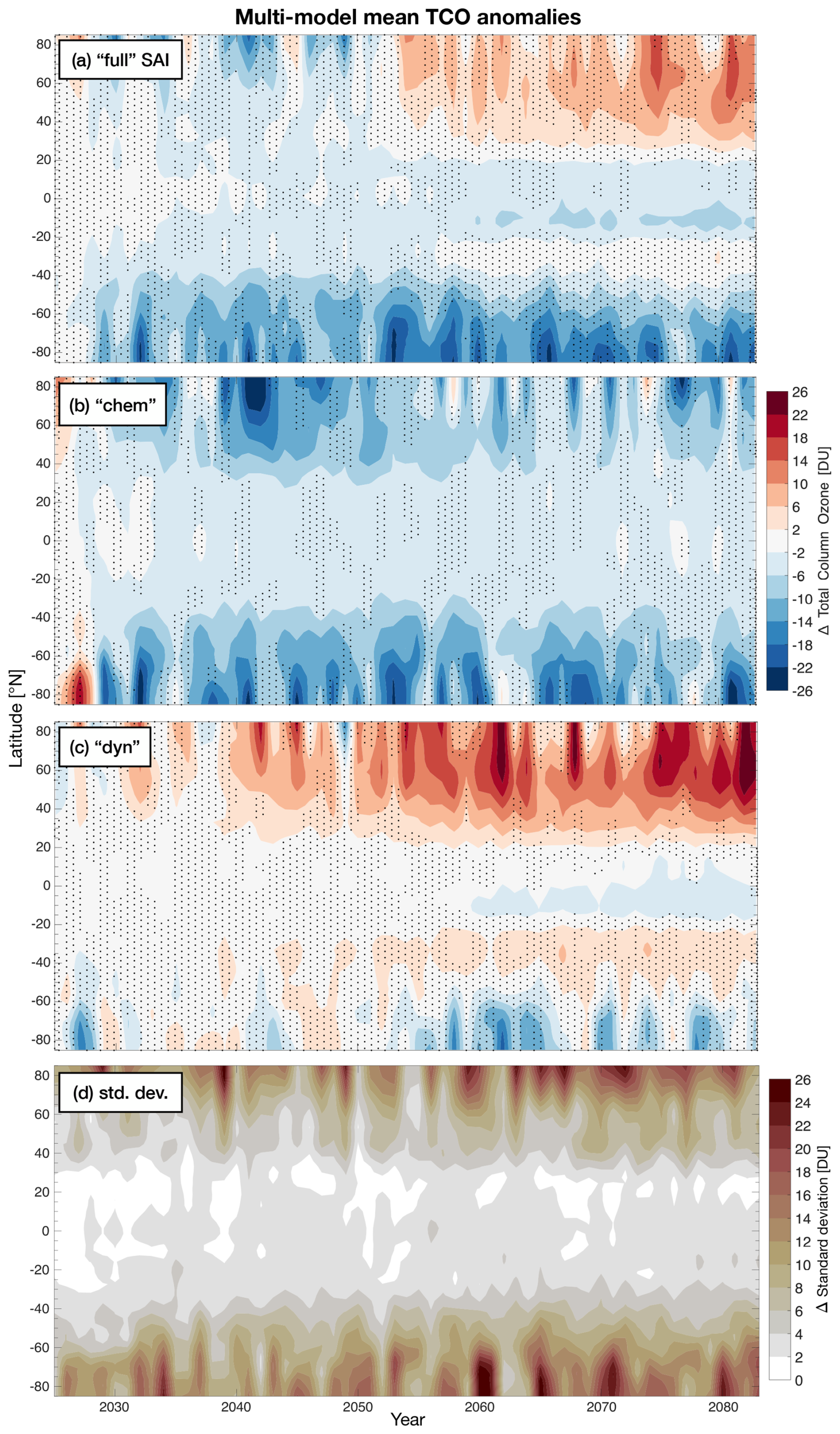
Figure 10 Multi-model mean zonal mean total column ozone anomalies due to full SAI (senD2-sai – senD2-fix; panel a), only chemical effects of SAI (“chem”; panel b), isolated dynamical effects (“dyn”; panel c) and the standard deviation of full SAI in panel (d). Panel (a) is the multi-model mean of all five models, panels (b) and (c), and (d) show multi-model means of the three models that simulated the senD2-chem simulation. The “full” some-model mean of the models that were used in panels (c) and (d) is not shown here, but added in Fig. C2. The standard deviation in panel (d) pertains to panel (a). Regions where the sign of all models do not agree are stippled.

Figure 9 resolves the intricate latitude-pressure pattern of ozone anomalies with height, where positive and negative anomalies are stacked above each other. This illustrates that SAI causes a major redistribution of ozone in the middle atmosphere (which has implications for stratospheric conditions), even in places, where the total column ozone does not change. Nevertheless, changes in TCO are a good indicator for changes in radiation received at the surface. In Fig. 10 we show the multi-model mean temporal evolution of TCO in Hovmöller plots; again including “full” (panel a) from all five models including standard deviation in panel (d) and “chem” and “dyn” for SOCOL, CMAM and NIES. A multi-model mean of these three models and their standard deviation is provided in Fig. C2. In the “full” multi-model mean the subtropics generally show little inter-model agreement in the sign of the anomaly (hatched regions). The tropics part reveals that the vertically stacked anomalies from Fig. 9a almost cancel out. Over time, a growing negative trend emerges, reaching up to around 8 DU of ozone depletion with some consistency across models. The negative effect of “chem” – as the ozone decrease in the lower stratosphere from halogen activation dominates over the ozone increase above it from NO_x deactivation – remains roughly constant with time in low-latitudes, as SAD increases but background halogen levels available for activation decrease with time. It is countered by “dyn” (which accounts for direct transport effects and thermodynamical influence on chemistry) at first, although models partially disagree in sign. By 2060, however, “dyn” also starts to add a significant negative contribution in the tropics, strengthening the chemical effect and leading to a combined negative anomaly of ∼ 5 DU in “full” by 2080. In the South, SAI causes ozone depletion throughout the entire simulated period that the models agree well on, despite inter-annual variability in polar conditions (polar vortex strength and temperatures). While there is still a positive signal in “dyn” in the Southern mid-latitudes from SAI-induced changes in both the shallow and deep branch of the BDC that balances the negative “chem” contribution, it wanes towards the South Pole. In contrast, the positive “dyn” anomaly frequently extends into polar latitudes in the North and grows considerably in strength over time, because the North pole is dynamically less isolated. This causes a transition from significant negative to significant positive TCO anomalies in the “full” multi-model mean. The transition occurs in the 2050s and marks a change in regime, where the positive TCO anomaly of altered dynamics dominates the negative chemical anomaly that is still persistent in “chem” even by the end of the century. Figure 10a shows that in addition to vertical ozone redistribution, competing effects also cause a hemispheric imbalance in the CCMI-2022 SAI scenario – even though the global mean TCO analysis (see Fig. 2c) largely suggests small global ozone changes in the second half of the 21st century for many models.

4 Synthesis and Outlook

4.1 Agreement and differences between models

In this analysis, we examined the chemical and dynamical response of the middle atmosphere to a specific SAI scenario with uniformly prescribed stratospheric aerosol properties in five models. This comparison primarily serves to highlight where the models agree well and to understand the characteristic features of individual models and where they diverge. Since this experiment eliminated differences from model-dependent aerosol microphysics modules, the remaining differences we show in this study indicate which other model components require further testing and development to improve multi-model projections under SAI. Overall, the models qualitatively agree very well on ozone concentration anomalies in different regions, which points to a good representation of the processes involved. The separation of processes using the additional senD2-chem simulation demonstrated that in many regions heating-derived effects, i.e., dynamical changes (transport response to temperature changes) and dynamically-induced changes in chemistry – which we also call nonlinear feedback effects – define the SAI response. Even though these effects, which contribute to ozone anomalies, appear regionally consistent across the five models analyzed, important uncertainties remain in their magnitudes. For one, the importance and persistence of chlorine activation – a key contributing factor to the ozone anomalies in the (polar) lower stratosphere – strongly varies across models (even when disregarding the high sensitivity in SOCOL), with SOCOL and NIES even showing opposite trends above the tropical tropopause compared to the other three models, in the form of an increase in ClO_x and decrease in HCl. High variability is also recorded in the polar lower stratosphere, where springtime total column ozone anomalies averaged over 60–90° latitude range from around −90 to −10 and −30 to +30 DU over the South and North Pole, respectively, by the year 2100. More variability between models, despite prescribing the same aerosol optical (radiative) properties in all models, is found in the rate of change in lower tropical stratospheric temperature, which ranges from just over 0.5 (CMAM) to just over 1 K (MIROC) per decade in Fig. 2b. The differences are correlated with the use of different radiation schemes. This results in a high variance in the transport of chemical species, especially in the tropical pipe. It is exemplified in MIROC that shows the strongest acceleration of the deep branch of the Brewer-Dobson circulation producing the highest CH₄ and N₂O increases in the upper stratosphere. For water vapor, in turn, SOCOL shows the highest positive percentage anomaly (over 50 %) in the lower stratosphere due to its large tropopause cold point warming, while NIES has a strong positive H₂O anomaly of some 30 % that extends up highest into the upper stratosphere. CMAM projects particularly strong NO_x passivation in the middle stratosphere and WACCM shows the smallest zonal wind anomalies, possibly due to its rather low equator-to-pole temperature gradient in the lower stratosphere. Due to these various features unique to specific models, the multi-model mean presented in this study should be interpreted with the experimental setup and the model spread in mind. Even still, the spatial pattern of ozone anomalies and thus the extent in latitude and altitude of the dominant processes controlling ozone in each region, is in remarkably good agreement across all models. There are various ways to investigate key differences between the models using more idealized simulations. To further isolate differences in heterogeneous chemistry, model experiments could be constrained by nudging the wind and temperature fields, in addition to fixed aerosol fields, thereby removing all dynamical differences among the models. Differences could arise from handling the production of nitric acid trihydrate and ice clouds, in both tropics and high latitudes, or differences in the heterogeneous reaction rates. In addition, radiative transfer schemes could be tested through offline calculations, while impacts of photolysis rates could also be tested, but only in models that can handle both prescribed and interactive photolysis schemes. A follow-up “dynamics-only” senD2-dyn simulation is also planned for a more elaborate analysis of the chemistry-transport-dynamical feedbacks.

4.2 Limitations of aerosol forcing implementation and future recommendations

Despite the best efforts of the CCMI-2022 experiment to eliminate differences in the aerosol forcing, some aspects of implementation in the models may have accounted for minor inconsistencies. Prescribing stratospheric aerosol derived from one model in another model poses a distinct challenge: the tropopause height is not necessarily the same. Consequently, if a stratospheric mask is applied to the aerosol data, some of the aerosol load may be truncated. This problem has not been addressed in this study, but in the future one could interpolate the stratospheric aerosol input onto the model-specific part of the stratosphere from the tropopause to an isotherm defining the aerosol evaporation threshold at every timestep to include the entire forcing. This method would also allow for the implementation of a full latitude-longitude-pressure field in any new experiments with a prescribed aerosol forcing. Accounting for zonal variations in the aerosol is secondary to meridional variations due to fast zonal mixing time scales, but could introduce a bias in heterogeneous chemistry. Processes like chlorine activation are limited by aerosol surface, the formation of which is sensitive to temperature and thus often appears regionally and bound to orographic features. Imposing a zonal mean aerosol forcing may not be sufficient to accurately reflect the occurrence and impact of heterogeneous chemistry. However, this would still not solve the problem of the inconsistency between the in-situ model transport barriers and the shape of the monthly mean aerosol forcing, which can result in different amounts of aerosol being taken into account within the wintertime vortex, important for ozone chemistry. This can be solved by reshaping the forcing along a potential vorticity coordinate system (i.e., using equivalent latitude instead of the geographic latitude-longitude grid).

Appendix A: Additional ozone anomalies

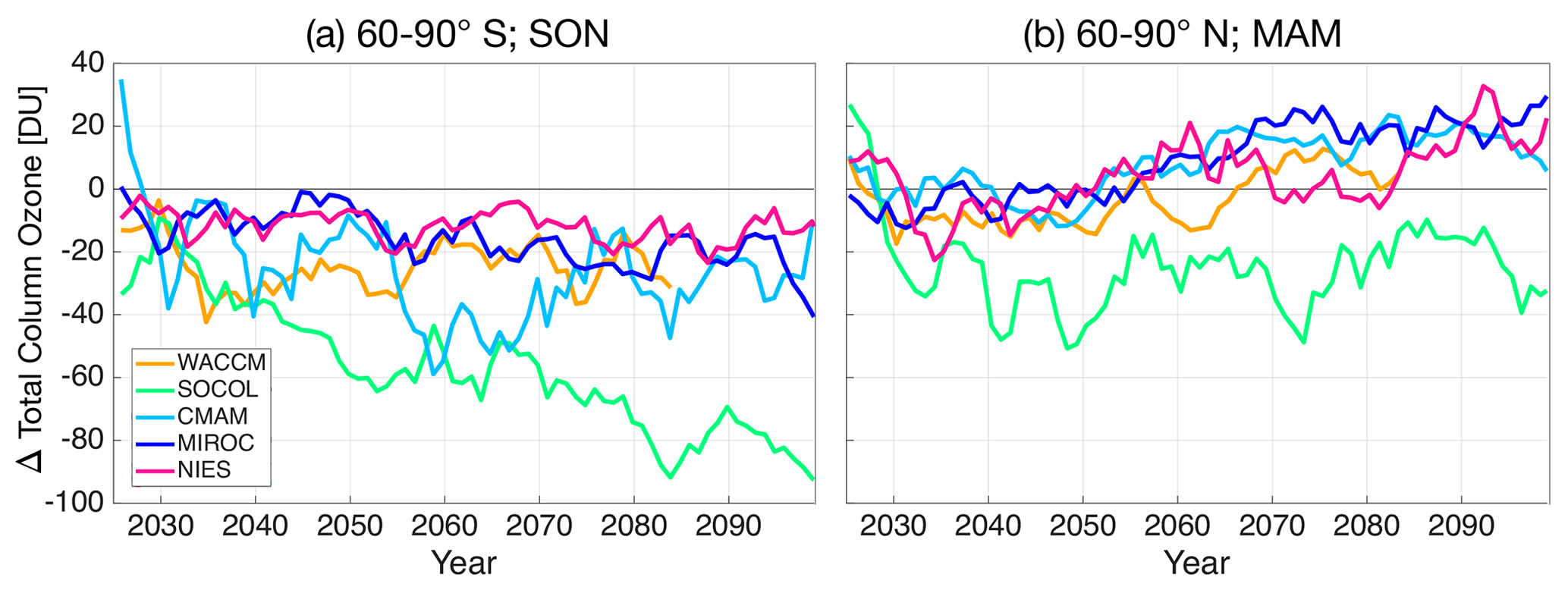
Figure A1 Mean total column ozone anomalies due to full SAI (senD2-sai – senD2-fix) from 60 to 90° S in austral spring (SON; panel a) and from 60 to 90° N in boreal spring (MAM; panel b). All timeseries have been treated with a moving mean filter of 5 years width.

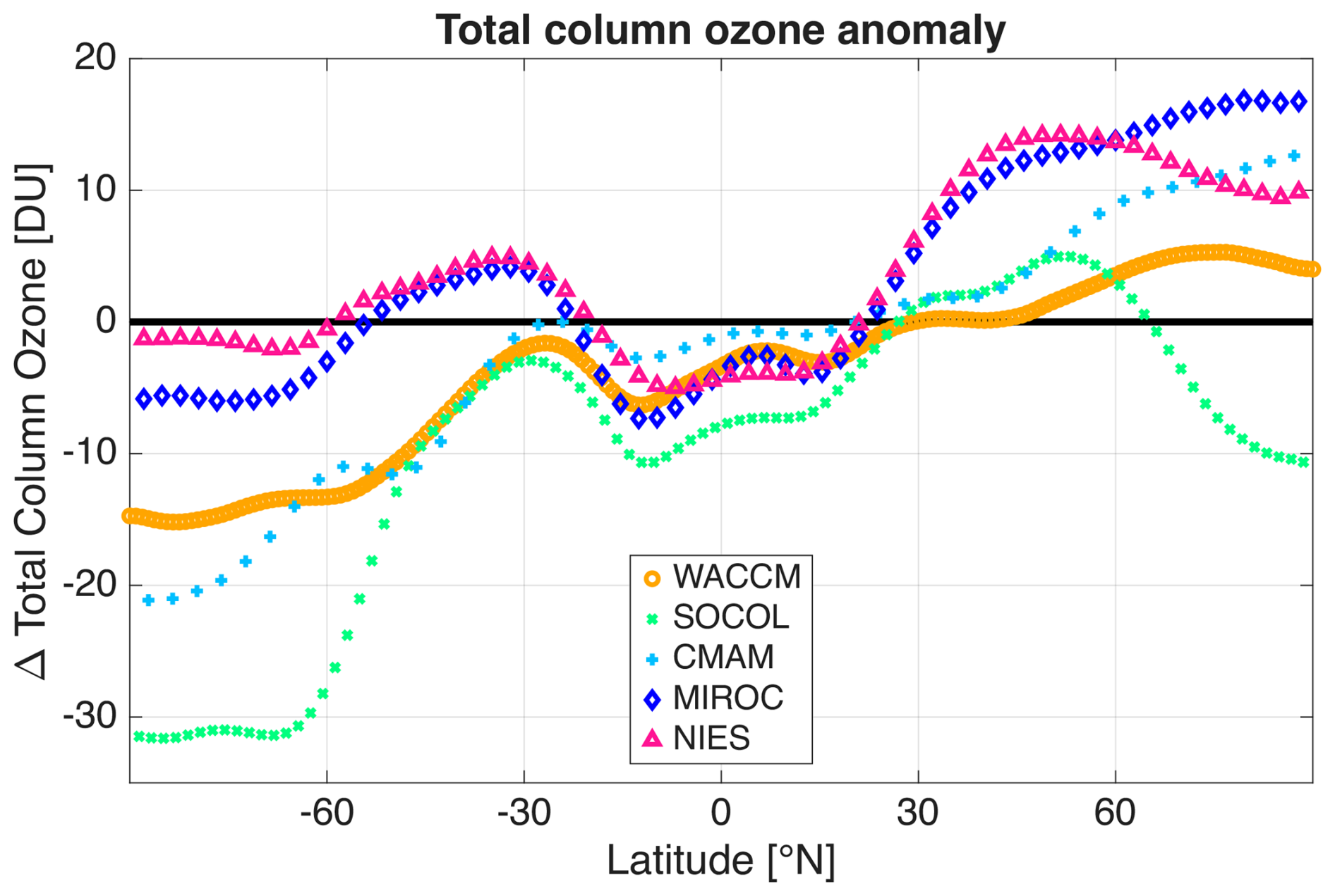
Figure A2 Mean total column ozone anomalies due to full SAI (senD2-sai – senD2-fix) from 2070–2083 as function of latitude.

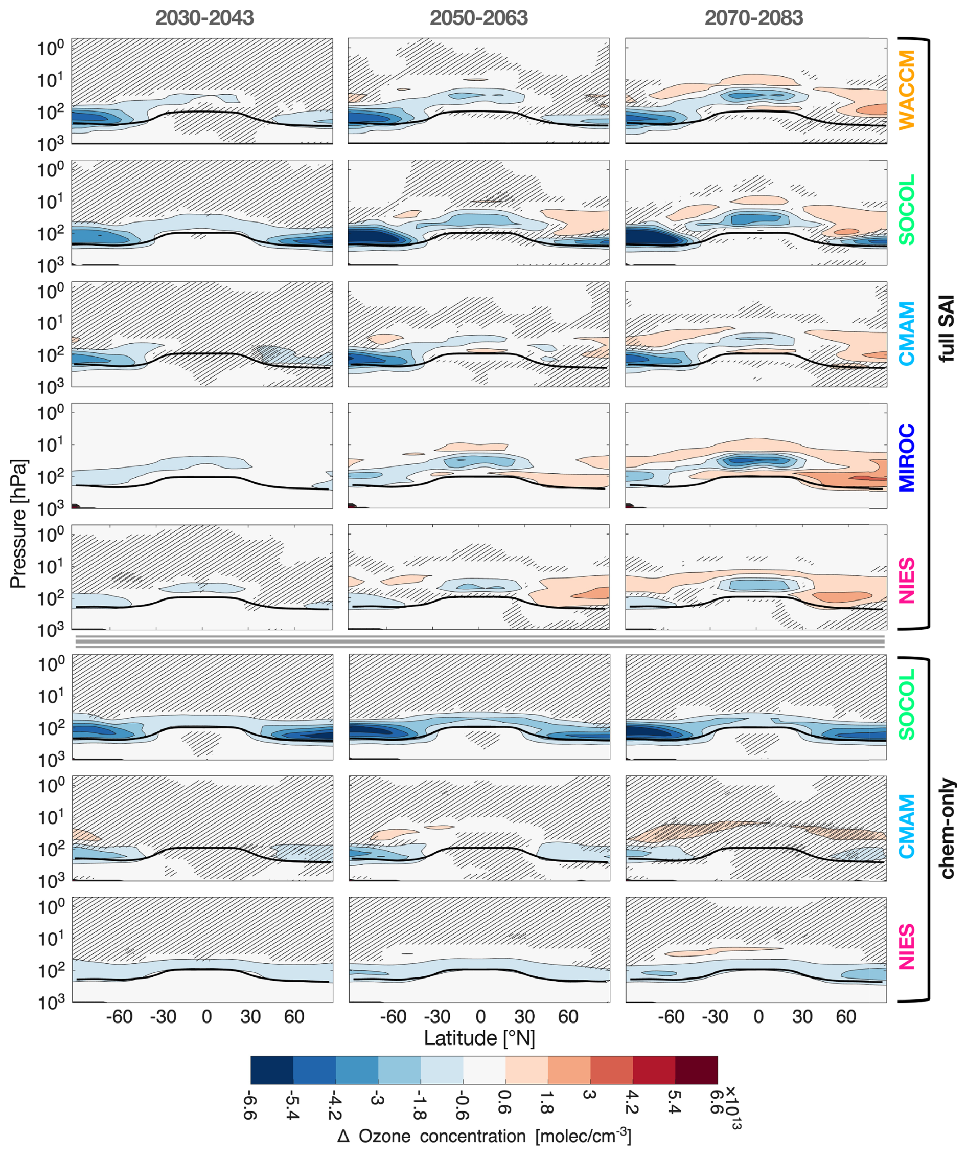
Figure A3 Zonal mean ozone number density anomalies in the full SAI scenario (senD2-sai – senD2-fix; top five rows) and for three of the models in the SAI chemistry-only scenario (senD2-chem – senD2-fix; bottom three rows). Anomalies are averaged over the 14-year time periods specified on top of each column. Black lines: mean senD2-sai tropopauses. Hatched areas: not significant at a 1 % level in a two-sample t-test.

Appendix B: Active families and reservoir gases percentage anomalies

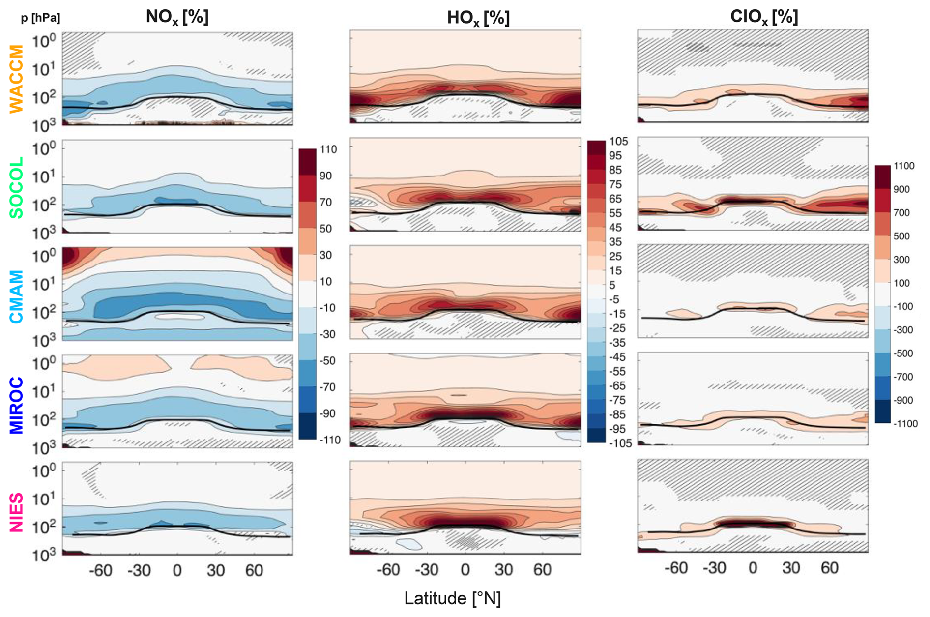
Figure B1 Zonal mean active nitrogen oxide (NO + NO₂ + 2 × N₂O₅), active hydrogen oxide (OH + HO₂), and active chlorine (oxide) (Cl + ClO + 2 × Cl₂O₂) percentage anomalies due to SAI [(senD2-sai − senD2-fix)/senD2-fix] for the 2060–2079 period. Black lines indicate the senD2-sai tropopause. Hatched areas are not significant at a 1 % level in a two-sample t-test.

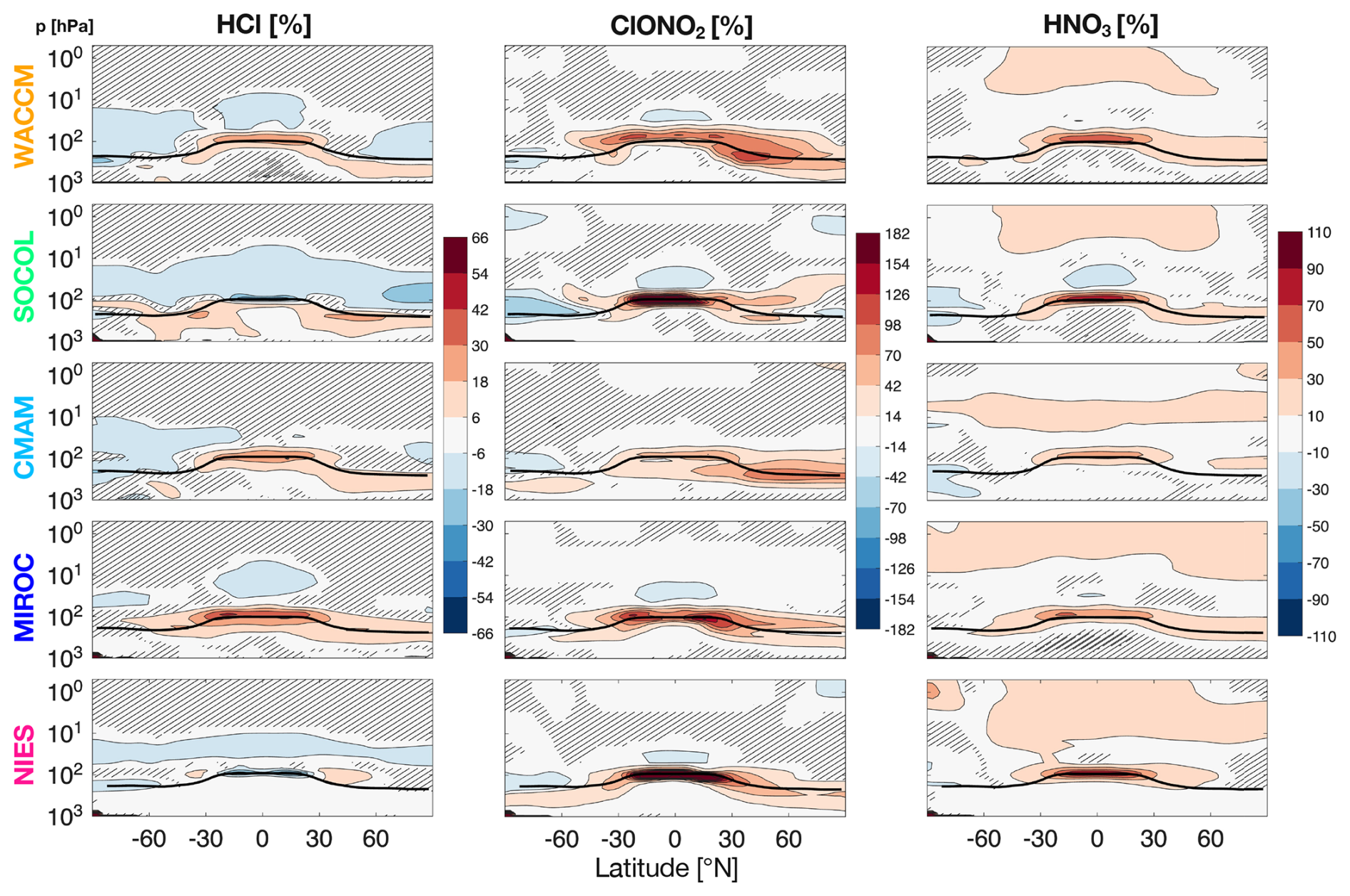
Figure B2 Relative zonal mean anomalies (in %) of hydrochloric acid, chlorine nitrate, and nitric acid mixing ratio [(senD2-sai – senD2-fix)/senD2-fix] caused by SAI for the 2060–2079 period. Black lines: senD2-sai tropopause. Hatched areas: not significant at a 1 % level in a two-sample t-test.

Appendix C: Three-model means

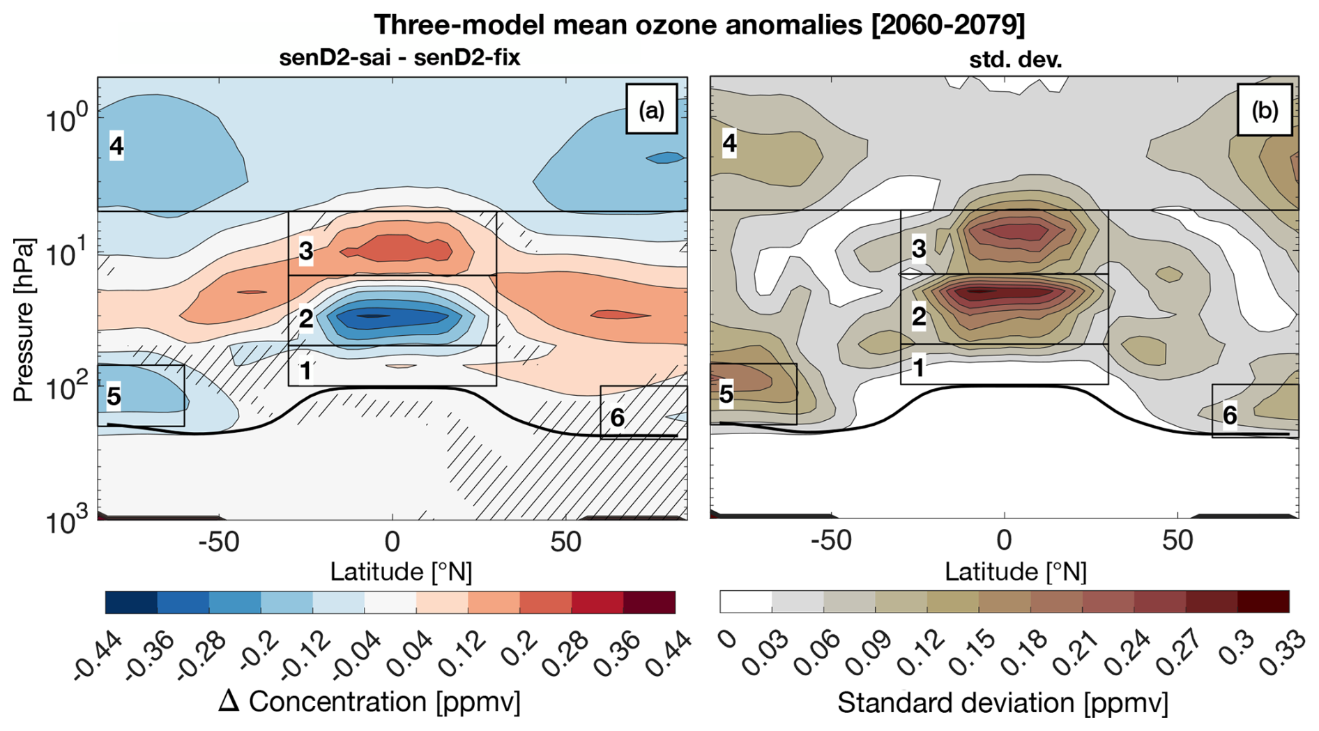
Figure C1 Three-model mean zonal mean ozone anomalies due to full SAI (senD2-sai – senD2-fix; panel a) and standard deviation in panel (b). Panel (a) is the multi-model mean of the three models that produced the chemistry-only simulations: SOCOL, CMAM, and NIES. These are the same models that are used to make the plots in panels (b) and (c) of Fig. 9. The black rectangles show regions with a dominant process shaping the ozone anomaly signal. The black line indicates the tropopause. Regions where the sign of all models do not agree are hatched.

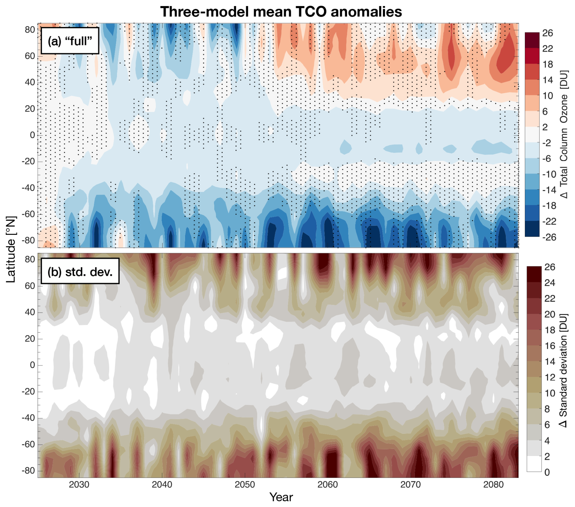
Figure C2 Three-model mean zonal mean total column ozone anomalies due to full SAI (senD2-sai – senD2-fix; panel a) and the standard deviation of full SAI in panel (b). Panel (a) is the multi-model mean of the three models that produced the chemistry-only simulations: SOCOL, CMAM, and NIES. These are the same models that are used to make the plots in panels (b) and (c) of Fig. 10. Regions where the sign of all models do not agree are stippled.

Appendix D: Heterogeneous chemical reactions

Table D1 Heterogeneous chemical reactions on aerosol surfaces included in the models. For each reaction the type of aerosol it is modeled on is listed. Note that CMAM does not include any NAT² chemistry. The table is comprehensive.

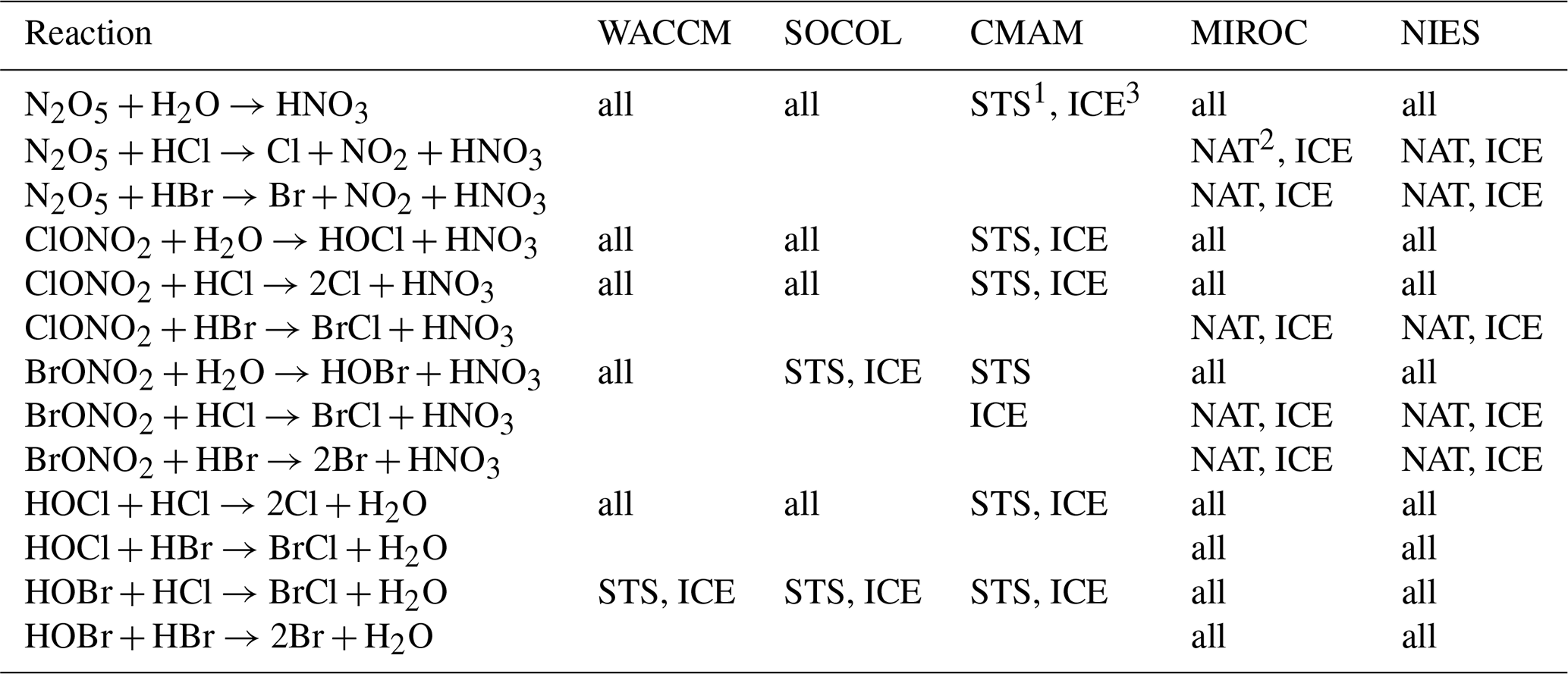
¹ supercooled ternary solution (liquid) aerosol, ² nitric acid trihydrate (solid) aerosol, ³ solid ice aerosol.