Assessment of the differences in European CH₄ emission estimates from three TROPOMI products

Satellite observations from the Sentinel-5P TROPOMI instrument, combined with inverse modeling, provide a valuable resource for quantifying regional methane (CH₄) emissions. This study compares the 2019 European emissions estimated from variational inversions assimilating three TROPOMI products of dry-column methane mole fractions (XCH₄). The SRON (v2.4, operational product), BLENDED (v1.0), and WFMD (v1.8) products are retrieved from distinct algorithms. These retrievals differ in coverage, error characterization, and XCH₄ spatial distribution. Machine learning predictions of XCH₄ differences point to aerosol scattering and albedo sensitivity as the largest contributors to the differences. The derived 2019 European CH₄ emission budgets show an increase of +2 % for SRON, and a decrease of −1 %, −33 % and −9 % relative to the prior, respectively, for BLENDED, WFMD and surface-based inversions. The range of budget estimates reveals inconsistencies in the total emissions derived from the inversions. At the national and sub-national scale, spatial emission patterns are similar for the non-independent SRON and BLENDED but differ substantially from WFMD. No inversion provides a systematically closer match to the spatial distribution of emissions derived from independent surface observations. Evaluation at surface stations shows that the residual between the observations and the posterior concentrations is reduced for 37 %, 53 % and 47 % of the stations, respectively, for SRON, BLENDED and WFMD. Observing System Simulation Experiments (OSSEs) are used to disentangle the drivers of differences between the posterior emissions. Results show that aligning coverage and individual observation errors increases the consistency between emission estimates. Residual differences in the OSSE posterior emissions can be attributed to differences in averaging kernels and prior profiles.

1 Introduction

The global emission pathways to limit global warming below the international objective of 1.5 °C (IPCC, 2021) include significant reductions of methane (CH₄) emissions. Methane is the second most important anthropogenic greenhouse gas (GHG) after carbon dioxide (CO₂). Despite its relatively short atmospheric lifetime of 9.1±0.9 years (Szopa et al., 2023), it has a strong radiative efficiency (Forster et al., 2021). The accounting of emissions is required to assess the current regulatory policies and to provide a robust reference for projections. For that, inverse modeling of CH₄ emissions combines atmospheric observations and transport simulations. This top-down (TD) approach complements bottom-up (BU) emission reporting by using independent information provided by atmospheric mixing ratios to reduce uncertainties on the emissions.

In the last decade, satellite data of CH₄ total column dry air mixing ratios (XCH₄) (Monteil et al., 2013; Cressot et al., 2014; Alexe et al., 2015; Bergamaschi et al., 2015) have provided wider spatial coverage than the surface data but with a double challenge: the estimation of the XCH₄ retrieval from the raw spectroscopic measurement, and the estimation of emissions based on the assimilation of retrievals. Satellite instruments can be divided into area flux mappers, designed to observe emissions at the global or regional scale, and point source imagers (Jacob et al., 2022). Point source imagers are fine-pixel instruments designed to quantify the point source emissions from the observation of the CH₄ plume. They are used to build datasets of local emitters (Schuit et al., 2023), available in public interactive tools such as the CAMS Methane Hotspot Explorer app and the Methane Alert and Response System (United Nations Environment Programme, 2025). Area flux mappers of methane include SCIAMACHY, launched on-board ENVISAT in 2002, the first instrument to provide global methane observations (Bovensmann et al., 1999); TANSO-FTS, launched in 2009 on-board the Greenhouse Gases Observing Satellite (GOSAT), that provides relatively accurate but sparse XCH₄ observations (Parker et al., 2020); IASI, on-board the MetOp satellites, a thermal-infrared (TIR) interferometer (Dils et al., 2024). The TROPOspheric Monitoring Instrument, also known as TROPOMI (Veefkind et al., 2012), launched in October 2017 on-board the satellite Sentinel-5P, now provides XCH₄ with a nadir resolution of 5.5 km × 7 km and daily global coverage (Hu et al., 2016; Hasekamp et al., 2022). Its high resolution (relative to other instruments) together with its high coverage make it possible to quantify both point source and regional/global CH₄ emissions. TROPOMI retrievals have been successfully used to detect large releases from oil and gas facilities (Schneising et al., 2020; Zhang et al., 2020; Lauvaux et al., 2022; Veefkind et al., 2023), as well as coal mines and landfills (Schuit et al., 2023) and large persistent source regions (Vanselow et al., 2024). They have also been used to quantify national and sectoral emissions, in global (Qu et al., 2021; Yu et al., 2023; East et al., 2025) and regional inversions for the US (Shen et al., 2022; Nesser et al., 2024), the Middle East and North Africa (Chen et al., 2023), East Asia (Chen et al., 2022; Liang et al., 2023) and South America (Nathan et al., 2024; Hancock et al., 2025). Small sources account in aggregate to a large proportion of total emissions at the national scale (Williams et al., 2025): bridging the gap between the local emission estimates and aggregated national budgets is a current challenge (Santaren et al., 2021; Naus et al., 2023).

The TROPOMI XCH₄ total columns are retrieved from SWIR radiance measurements along with the averaging kernels (AKs), that assess the sensitivity of the retrievals to the different atmospheric layers. This derivation is a major challenge: the retrieved columns and the vertical sensitivity indeed strongly depend on the chosen algorithm and on different factors of the radiative transfer (e.g., clouds, the assumed prior profile of the CH₄ dry air mixing ratio, surface albedo and aerosols). The systematic analysis of the TROPOMI XCH₄ data has pointed to biases linked to albedo and scattering due to the presence of aerosols (Barré et al., 2021).

In this context, several products of TROPOMI XCH₄ retrievals have been developed with different algorithms, and they are iteratively updated. The SRON Netherlands Institute for Space Research provides the operational Copernicus product (Apituley et al., 2025), which has been updated with the optimized settings of the research product (Lorente et al., 2021, 2023). It uses the full-physics algorithm RemoTeC and simultaneously retrieves XCH₄, surface albedo and atmospheric scattering properties. A destriping algorithm, based on moving median smoothing in the across-track directions and flight directions, has been developed for new XCH₄ data (Borsdorff et al., 2024). The BLENDED TROPOMI+GOSAT product (Balasus et al., 2023) is a corrected version of the SRON product. It relies on a machine learning model, trained to predict the differences between TROPOMI and GOSAT co-located retrievals. The modeled correction was applied to the whole SRON dataset. The scientific WFMD product from University of Bremen is independent of the other two and is based on the algorithm Weighting Function Modified Differential Optical Absorption Spectroscopy (WFMD-DOAS) (Schneising et al., 2019, 2023).

Previous inter-comparisons only include the SRON and WFMD products (Hilbig et al., 2023). A comparison of observations at high latitudes (Lindqvist et al., 2024) revealed higher XCH₄ for WFMD in comparison to SRON, as well as a persistent seasonal bias for the SRON (high values in spring, low values in autumn). The assimilation of older versions of SRON and WFMD products at high latitudes showed similarities but also clear differences in the posterior emissions, in terms of spatial and temporal distributions (Tsuruta et al., 2023). Despite the advancements in XCH₄ retrievals in recent updates and the additional product BLENDED, the literature on systematic comparisons between the products and between the estimated emissions remains limited.

This study aims at addressing these limitations by providing a comparison of CH₄ emissions estimated from the assimilation of the SRON, BLENDED and WFMD products in regional inversions. The objective is to assess the consistency of emission estimates, with respect to the aim of building emission inventories at the pixel, country and continental scale. This benchmark requires the characterization of the (in)consistencies in the observation coverage, observation errors and spatial biases of XCH₄ between the three datasets. The study covers the year 2019 and focuses on Europe, where an extensive network of surface stations provide independent CH₄ measurements that are used to support the comparison.

First, we compare the three products over Europe in 2019. We investigate the role of atmospheric, instrumental and algorithmic variables in driving the XCH₄ differences between products. Using a machine learning model, feature contributions to the prediction of the differences are quantified, following the methodology of Balasus et al. (2023).

Subsequently, we perform variational inversions to estimate the CH₄ fluxes at a 0.5° × 0.5° spatial resolution and weekly temporal resolution by assimilating each product independently. We conduct Observing System Simulation Experiments (OSSEs) with synthetic pseudo-observations and perturbed prior fluxes. The OSSEs assess the ability of the inversion system to refine emission estimates and its sensitivity to parameters such as observation density, error characteristics, and inter-product differences. Scenarios focusing on specific changes provide insights into the drivers of differences in the posterior fluxes. We also investigate the role of the optimization of the boundary conditions and the stratospheric concentrations, but do not further address the question of model errors and their potential correlations with retrieval errors. Finally, we compare European CH₄ emission estimates in 2019 from the three TROPOMI products and ground-based observations, at the pixel, country, and regional resolution, to assess the consistency of the results at these various scales. For this study, we use the recent inverse modeling platform Community Inversion Framework (CIF Berchet et al., 2021), coupled with the regional Eulerian atmospheric chemistry-transport model (CTM) CHIMERE (Menut et al., 2013; Mailler et al., 2017) and its adjoint code (Fortems-Cheiney et al., 2021). CHIMERE has already been used to model transport of GHGs at the regional scale, especially CO₂ (Broquet et al., 2011; Santaren et al., 2021) and CH₄ (Pison et al., 2018). The methane observations, the configuration of the CHIMERE CTM and the methodology for the variational inversions and OSSEs are described in Sect. 2. The results, particularly those from the inversions and the OSSEs, are detailed in Sect. 3.

2 Data and Methods

The purpose of our atmospheric inversions is to correct prior estimates of the CH₄ emissions, to improve the fit between the simulations of CH₄ atmospheric mixing ratios by a CTM and the observations. In this section, we detail the inputs and components of the CIF-CHIMERE inversion system. Section 2.1 provides an overview and a comparison of the coverage, distribution and errors of the three TROPOMI products. It also introduces the other CH₄ observations used in this study. Section 2.2 describes the prior emission estimates, and Sect. 2.3 details the configuration of the CHIMERE CTM. The methodology for the inversions and OSSEs is outlined in Sect. 2.4.

2.1 CH₄ observations

2.1.1 TROPOMI satellite products

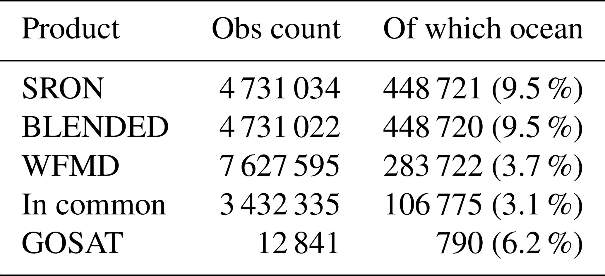
TROPOMI is on-board Sentinel-5 Precursor (S5P) since 2017. The radiances measured in the shortwave infrared range (SWIR, 2314–2382 nm) are used to derive methane total columns. The pixel size at nadir was about 7.2 × 7.2 km² before 2019/08/06. It was upgraded to 5.6 × 7.2 km² after a change in the instrument settings on this date. The swath is about 2600 km on ground, allowing global daily coverage. The accuracy requirements for XCH₄ total columns are 1 % bias and 1 % random error, as defined in the S5P Calibration and Validation Plan (European Space Agency, 2017). In this study, the assimilated methane retrievals consist of three level 2 (L2) products, described in the following sections. Table 1 shows the number of observations available in the domain in 2019 for each of these products.

Table 1 Number of available observations over the domain in 2019, for the three TROPOMI products SRON, BLENDED and WFMD used in this study, the “common” dataset (composed of the observations shared across the three TROPOMI products), and GOSAT.

SRON

The operational TROPOMI product (v2.4), hereafter called “SRON”, is developed by the SRON Netherlands Institute for Space Research. It includes the iterative improvements of the research product (Lorente et al., 2021, 2022), in particular better accounting for surface reflectance (Lorente et al., 2023). In this study, we use the reprocessed albedo bias-corrected version and apply the recommended filtering criteria (Apituley et al., 2025) to ensure high-quality data (quality flag superior to 0.5). This product is retrieved from TROPOMI measurements with the RemoTeC full-physics algorithm, that retrieves both the atmospheric methane mixing ratio and the physical scattering properties of the atmosphere. A detailed description of the algorithm is given in the Algorithm Theoretical Baseline Document (Hasekamp et al., 2022). A destriping procedure (Borsdorff et al., 2024) is applied to new XCH₄ data from 7 September 2024 (v2.07), but older orbits have not been reprocessed. This empirical approach consists in removing the CH₄ background by a median smoothing in the cross-track direction, and then computing a per orbit stripe value as a median in the flight direction, which is used for correction (Borsdorff et al., 2019). However, this processing is not applied to the 2019 observations used in this study.

Blended GOSAT+TROPOMI product

The BLENDED product (Balasus et al., 2023) is a corrected version of SRON: a machine learning (ML) model has been trained to predict the differences between GOSAT and TROPOMI-SRON (v2.4) observations, based on SRON data features. The GOSAT XCH₄ product uses a proxy retrieval which is less sensitive to surface and atmospheric artifacts. It is described in further detail in Sect. 2.1.2. The global mean bias versus TCCON data (9.2 ppb) is subtracted from all GOSAT observations (Parker et al., 2020). The correction is modeled on co-located observations, then applied to the whole TROPOMI-SRON record. This method aims at taking advantage of the density of TROPOMI measurements, while mitigating the effect of known biases associated to surface albedo, coarse aerosol particles and striping, thanks to the GOSAT proxy approach. We keep only the highest quality data (quality flag of 1) and filter for coastal scenes as recommended by Balasus et al. (2023). This quality filter is theoretically stricter than the one recommended for the SRON product, but in practice it eliminates only 12 observations over the domain in 2019. It can thus be considered that both SRON and BLENDED products share the same observation sampling (see Table 1). In the BLENDED product, the observation errors, averaging kernels and prior profiles are directly taken from the SRON product (only the XCH₄ values differ between the two products).

WFMD

The WFMD scientific product v1.8 (Schneising et al., 2019, 2023), hereafter called “WFMD”, is based on the Weighting Functions Modified Differential Optical Absorption Spectroscopy (WFMD-DOAS). Quality filtering is based on a random forest (RF) classifier: data with a quality flag of 0 is selected. Post-processing includes systematic bias correction (eg. due to albedo) based on a RF regressor, as well as a destriping filter based on combined wavelet–Fourier filtering.

Common observations

To separate the effect of varying coverage between products from the effect of the differences in the XCH₄ distributions, we extract a dataset of observations shared across all three products, so that they have identical spatio-temporal sampling. This “common” dataset is used for the analysis of the inter-product differences (Sect. 3.1) and for OSSEs (Sects. 2.4.3, 3.4).

2.1.2 Other CH₄ observations

In Sect. 2.1.3, we compare TROPOMI observations with retrievals from the University of Leicester GOSAT Proxy XCH₄ product, v9.0 (Parker et al., 2020). The GOSAT satellite was launched in 2009. Methane estimates are based on the CO₂ proxy method, which takes advantage of CO₂ absorption in the measured 1.65 µm band, with a finer spectral resolution than TROPOMI. This approach significantly reduces the error in the retrieval, since it cancels aerosol and surface artifact contributions that similarly affect XCO₂ and XCH₄ measurements. Only highest-quality data (quality flag of 0) is considered, yielding 12 841 observations over the domain in 2019. The global mean bias versus TCCON data is removed from the GOSAT observations shown in the following, subtracting 9.2 ppb from all retrievals, to be consistent with the dataset used by Balasus et al. (2023) to derive the BLENDED observations (see Sect. 2.1.1).

To evaluate the results of the inversions, we use independent in-situ measurements of CH₄ mixing ratios from flasks and continuous sampling sites. The 19 available surface sites for 2019 are listed in Table A1. The data are compiled from the ICOS atmospheric network (https://www.icos-cp.eu, last access: March 2025), the World Data Centre for Greenhouse Gases (WDCGG, https://gaw.kishou.go.jp, last access: March 2025), the NOAA ESRL discrete sampling network (https://www.esrl.noaa.gov/gmd/, last access: March 2025) and the EBAS data base. Data from sites with continuous measurements are averaged to hourly values. The evaluation consists in comparing the emissions derived from the satellite-based inversions to an inversion assimilating only these surface measurements (Sect. 3.3). We also compare the posterior simulated concentrations at the locations of the surface stations to these independent measurements (Sect. 3.5).

2.1.3 Comparison of the TROPOMI XCH₄ coverage, distribution and errors

Coverage

The inter-comparison of TROPOMI satellite retrievals reveals differences in coverage over Europe in 2019. The density of observations is a critical parameter for ensuring robust constraints on emissions during the inversion. Yet, substantial differences exist between SRON/BLENDED and WFMD, as shown in Table 1. WFMD exhibits 63 % more observations in comparison to SRON and BLENDED over Europe in 2019. This higher observation count is attributable to the different filtering approaches: as mentioned in Sect. 2.1.1, WFMD employs machine learning techniques to identify scenes that are poorly characterized by the retrieval algorithm (Schneising, 2023); quality control criteria for SRON and BLENDED rely on threshold-based filters for cloud fraction, solar zenith angle and other scene description variables (Landgraf et al., 2025).

The temporal coverage shows consistent variations for the three products (Fig. 1a): observation density is high between June and October and decreases during winter. An anomalously low density is noticeable for all products in May 2019. It is due to an increase of the Fractional Cloud Cover (CFC) over Europe during this month, as indicated by the CLARA-A3 record (Karlsson et al., 2023). Seasonal spatial variations are consistent among products, with an absence of observations at high latitudes (≳60°) during winter months (see Fig. S1 in the Supplement).

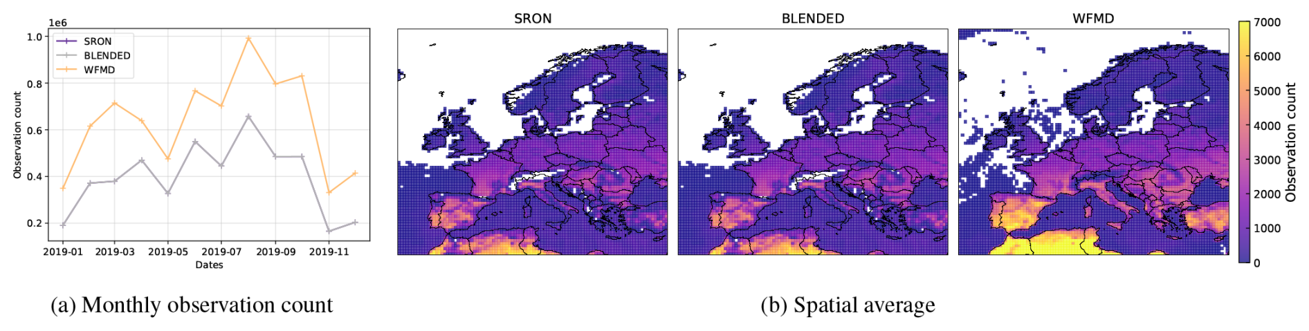
Figure 1 Number of observations per month (a) and per 0.5° longitude × 0.5° latitude cell 2019 (b) for the three TROPOMI products SRON, BLENDED and WFMD used in this study. The covered period includes the change in pixel size (7.2 to 5.6 km) in the along track direction, starting on the 6 August 2019.

Spatial patterns of coverage differences are illustrated in Fig. 1b. The WFMD dataset demonstrates a higher density of observations in arid regions (e.g., over Spain and Turkey). Moreover, it includes a few observations in mountainous areas (Alps, Norway), whereas SRON and BLENDED filter out all retrievals in these regions.

Comparison of TROPOMI observations

The temporal and spatial XCH₄ distributions of the three products are shown in Fig. 2. Average observed XCH₄ in 2019 is respectively 1850, 1843 and 1856 ppb for SRON, BLENDED and WFMD (Fig. 3). Part of the differences between the distributions can be explained by the differences in spatial coverage between SRON/BLENDED and WFMD. When considering only the common observations across the three datasets, the average XCH₄ are slightly closer but still differ (1851, 1844 and 1856 ppb respectively), and the analysis of space-time distributions remains similar.

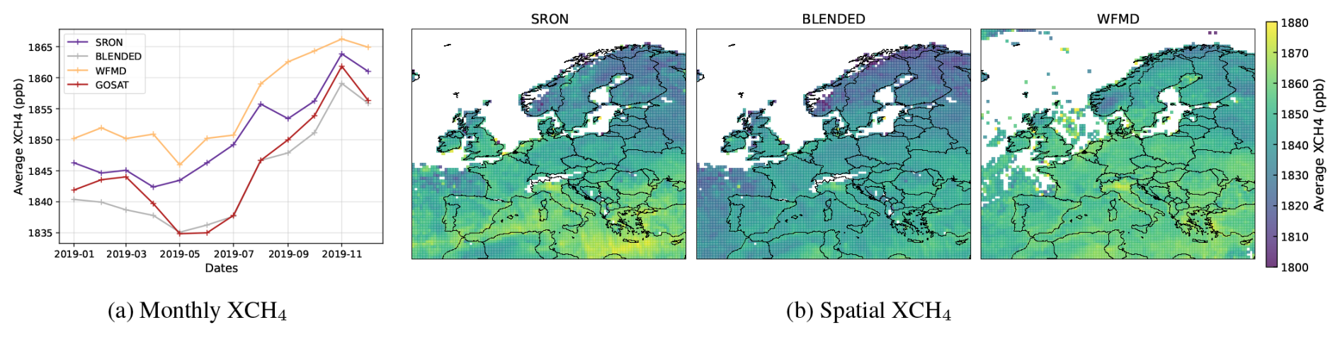
Figure 2 Average XCH₄ observation per month (a) and per 0.5° × 0.5° cell in 2019 (b) for the three TROPOMI products.

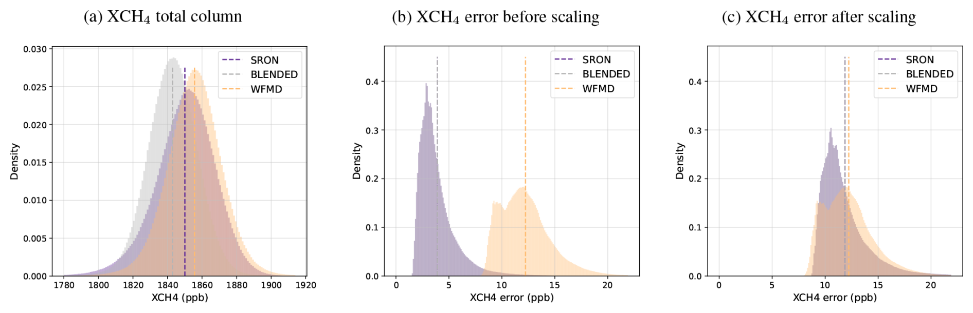
Figure 3 Distributions of observations (a) and observation errors (b, c), both in pbb, for the three TROPOMI products. For the error, panel (b) shows the raw errors, while panel (c) shows the same histogram after error scaling for the SRON and BLENDED products. SRON and BLENDED errors are exactly similar, as BLENDED errors are directly retrieved from the SRON product.

The temporal variations of XCH₄ throughout the year show overall similar shapes (Fig. 2a). Average concentrations decrease slightly from January to May, reaching a minimum in April/May, before rising during late summer and autumn, peaking in November. The difference between BLENDED and WFMD monthly averaged values is steady over the year ($-\mathrm{11.7}\pm \mathrm{2.1}$ ppb). The differences between SRON and BLENDED (6.8±2.3 ppb), as well as SRON and WFMD ($-\mathrm{5.0}\pm \mathrm{2.5}$ ppb) depict more temporal variations: SRON observations tend to be closer to GOSAT and BLENDED in winter, but closer to WFMD in summer. Only BLENDED aligns rather well with GOSAT, due to its correction of the TROPOMI-GOSAT bias.

Overall, the spatial patterns of the distributions of CH₄ concentrations are consistent, yet with local discrepancies, e.g., in Scandinavia (higher XCH₄ than SRON for WFMD and lower for BLENDED, as seen in Fig. 2b). BLENDED shows lower XCH₄ over the domain, but also consistent spatial gradients with SRON and WFMD (Figs. 2b, S2).

To understand the drivers of the differences in XCH₄ distributions, we adopt the method outlined by Balasus et al. (2023). A machine learning (ML) model is trained to predict the difference in XCH₄ based on the retrieval variables. The contribution of individual features to the prediction is assessed to estimate the importance of each variable. The results and analysis of the biases are presented in Sect. 3.1. Detailed study of the differences of XCH₄ relative to TCCON is available in Appendix C.

Observation error

The retrieval error (in terms of uncertainty) attributed to individual observations can impact the emissions from inversions by changing their spatial and temporal variations (Lu et al., 2025b), as well as call into question both very high and very low emission values (Zheng et al., 2026). The definition of this error differs between the SRON/BLENDED and WFMD products. For SRON (thus also for BLENDED, for which only XCH₄ values are corrected), the reported error is defined as the standard deviation of the retrieval noise, which follows from the error covariance matrix in the retrieval inversion procedure. This error describes the effect of the noise in the measured radiances on the retrieval (Lorente et al., 2021). For WFMD, the error is propagated in the retrieval algorithm from the noise in the measured spectra. In both cases, the characterized error σ only includes the effect of noise in the measured radiance, however the unknown noise components related to atmospheric conditions or instrumental features are not accounted for.

To avoid underestimating the observation uncertainty, the products have different error corrections, based on the validation of the satellite XCH₄ with respect to total columns observations of the ground-based TCCON stations. SRON and BLENDED provides the error σ as described before and suggest to multiply it with a factor 2 to reflect the scatter of errors in the TCCON validation (Landgraf et al., 2025). We apply this recommended correction. For WFMD, the error σ is linearly rescaled, based on a regression of the scatter relative to TCCON observations (Eq. 1). The scaled error $\widehat{\mathit{\sigma }}$ is directly provided in the product and described in the Algorithm Theoretical Baseline Document (Schneising, 2023).

$$\begin{array}{}\text{(1)}& \widehat{\mathit{\sigma }}=\mathrm{4}/\mathrm{3}(\mathit{\sigma }+\mathrm{5}\mathrm{ppb})\end{array}$$

Due to this difference in error definition between SRON/BLENDED and WFMD, the errors of SRON and BLENDED (3.9 ppb in average) are smaller by a factor of 3 than those of WFMD (12.2 ppb) (Fig. 3b). If we try to apply the linear transformation of Eq. (1) to SRON/BLENDED errors, the resulting error distribution aligns more closely with WFMD: the average scaled error is 11.9 ppb for SRON and BLENDED (Fig. 3c). Therefore, the difference in rescaling the error based on the scatter relative to TCCON is the main source of difference in the final uncertainty provided in the products. The impact of this difference on the results of inversions is further evaluated in Sect. 3.4.

Vertical parameters

As illustrated in Fig. 4 (only the common observations are considered here), the column averaging kernels (AKs) and prior profiles exhibit similar shapes, characteristic of SWIR retrievals. The per level relative difference between SRON/BLENDED and WFMD vertical profiles is below 5 % for all levels. The WFMD AKs seem to be less sensitive to the layers close to the surface in comparison to SRON/BLENDED, but more sensitive to the stratosphere (pressures inferior to 200 hPa). Differences up to approximately 200 ppb occur between the prior profiles of SRON/BLENDED and WFMD, in particular for the layers close to the surface: the WFMD prior profiles are scaled to have uniform surface values of 1850 ppb, while SRON/BLENDED prior mixing ratios at the surface are between 1900 and 2000 ppb. The scaling of prior profiles for WFMD also explains the lower variability of prior mixing ratios in comparison to SRON/BLENDED, as evidenced by the narrower horizontal deviations in the right panel of Fig. 4. These profiles are consistent with the ones presented in Lindqvist et al. (2024), which also highlight a systemically higher prior profile for SRON in comparison to the one of WFMD. The differences in the profiles lead to differences in the simulated XCH₄ distributions, as shown in Sect. 3.2.

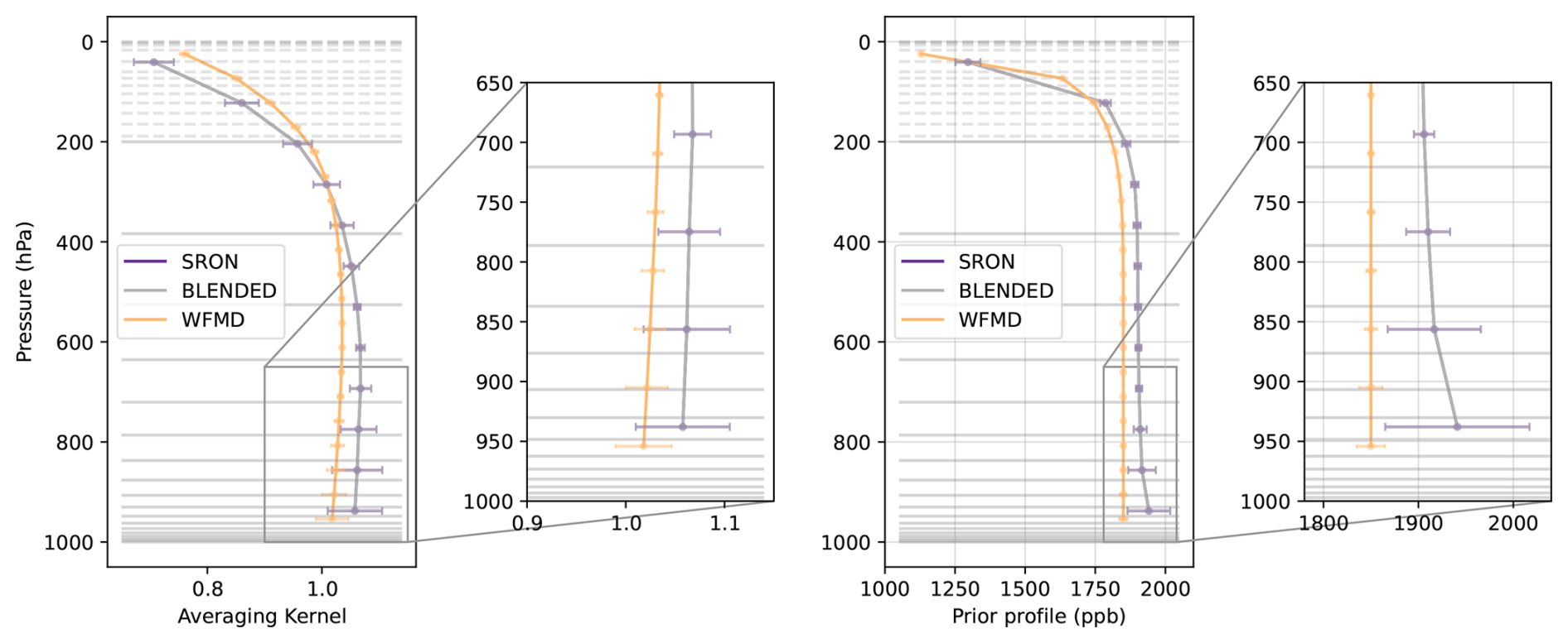
Figure 4 Column averaging kernels (left, unitless) and prior profiles (right, in ppb) averaged between the common observations of the TROPOMI products (dataset described in Sect. 2.1.1). The zoomed windows show the lower levels. SRON and BLENDED have exactly the same profile, since the only difference in the co-located dataset is the XCH₄ value. Horizontal lines are CHIMERE pressure levels (plain lines) and CAMS pressure levels in the stratosphere (dashed lines, for pressures lower than 200 hPa), for a surface pressure of 1000 hPa.

2.2 Prior estimates of the CH₄ emissions

Prior methane emissions are compiled from several BU inventories. Anthropogenic emissions are from EDGARv8.0 (Crippa et al., 2023). The biomass burning fluxes are taken from GFEDv-4.1s (Randerson et al., 2017). Natural fluxes consist of an ensemble of datasets provided by the Global Methane Budget protocol for inversions (GCP-CH₄, Saunois et al., 2020). Fluxes from wetlands (peatlands, inundated and mineral soils) are from the JSBACH-HIMMELI model (Raivonen et al., 2017). The geological emissions are a climatology based on Etiope et al. (2019) and scaled down to a global total of 15 TgCH₄ yr⁻¹ in accordance with the maximum suggested by Petrenko et al. (2017). The emissions due to termites are a climatology based on the estimate of S. Castaldi, from GCP-CH₄ (Saunois et al., 2020). Finally, the ocean fluxes are a climatology based on Weber et al. (2019). All these datasets have been interpolated at the 0.5° × 0.5° horizontal resolution of the CTM grid. The map of total emissions in 2019 is shown in Fig. 5. Anthropogenic emissions contribute to about 72 % of the total emission budget (25.2 TgCH₄ in 2019) for the countries listed in Table B1.

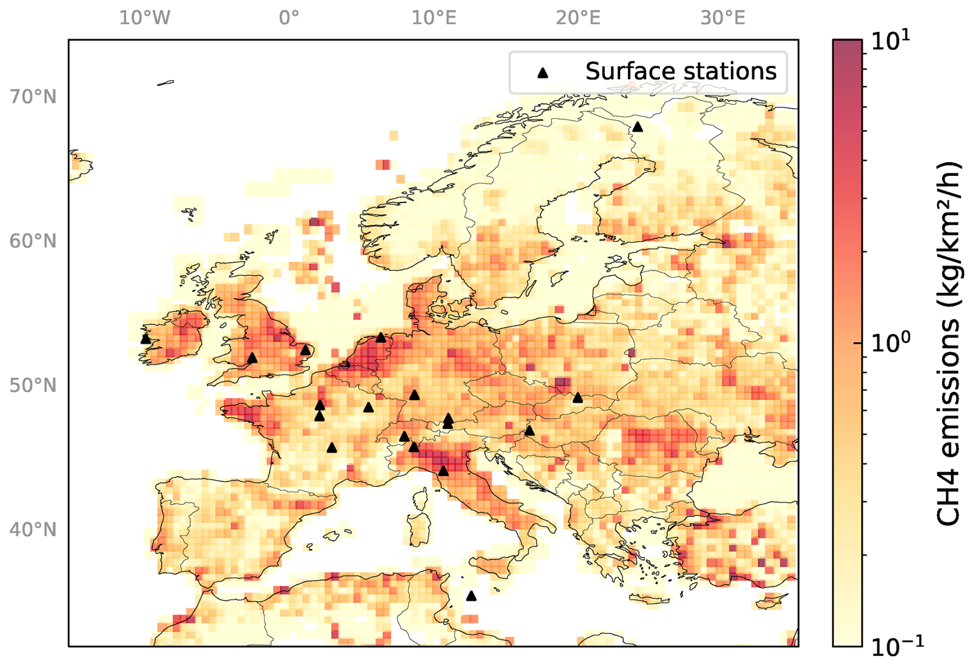
Figure 5 Prior CH₄ emissions (kg m⁻² h⁻¹) in Europe in 2019, in log-scale. Black triangles are the locations of the surface stations listed in Table A1.

2.3 Configuration of the CHIMERE CTM for the simulation of CH₄ concentrations

The CTM used for inversion is the regional chemistry-transport model CHIMERE (Menut et al., 2013; Mailler et al., 2017) and its adjoint code (Fortems-Cheiney et al., 2021). The targeted domain spans from 15° W to 35° E and 32 to 74° N. This domain has already been used for the intercomparison of inversions EUROCOM (Monteil et al., 2020). The grid used for discretizing emissions, meteorological data and other inputs and for running the CTM covers this domain at a 0.5° longitude × 0.5° latitude resolution. Vertically, the domain where transport is simulated by CHIMERE extends from the surface to 200 hPa (with 17 sigma-pressure levels). Above this pressure (approximately the tropopause) and up to 0.1 hPa, CH₄ concentration fields are taken from the CAMS reanalysis simulations (based on the Integrated Forecasting System (IFS) system of the European Centre for Medium-Range Weather Forecasts (ECMWF)) (Agustí-Panareda et al., 2023). Lateral boundary and initial conditions of methane mixing ratios are taken from the same CAMS product.

CHIMERE requires a set of meteorological variables, taken from the ECMWF IFS operational forecast (every three hours) retrieved at 0.25° × 0.25° and interpolated onto the model's grid. The size of the domain makes it possible to neglect the chemistry of CH₄ because its oxidation by hydroxyl radicals leads to a lifetime from 8 to 10 years (Saunois et al., 2020), whereas the ventilation time of the domain is of the order of 10 d (Nygård et al., 2023).

2.4 Variational inversions in the CIF-CHIMERE inversion system

2.4.1 Principle of Bayesian variational inversion

In the following, we use notations according to the convention defined by Ide et al. (1997) and Rayner et al. (2019). The 4D-Var inversion adjusts the control vector x, to improve the fit between observed satellite data and their simulated equivalents, by minimizing the cost function J:

$$\begin{array}{}\text{(2)}& \begin{array}{rl}J\left(\mathit{x}\right)& ={\displaystyle \frac{\mathrm{1}}{\mathrm{2}}}(\mathit{x}-{\mathit{x}}^b{)}^T{\mathbf{B}}^{-\mathrm{1}}(\mathit{x}-{\mathit{x}}^b)\\ & +{\displaystyle \frac{\mathrm{1}}{\mathrm{2}}}\left(\mathcal{H}\right(\mathit{x})-{\mathit{y}}^{\mathrm{0}}{)}^T{\mathbf{R}}^{-\mathrm{1}}(\mathcal{H}\left(\mathit{x}\right)-{\mathit{y}}^{\mathrm{0}})\end{array}\end{array}$$

where x^b and y⁰ are respectively the vector of prior information and the vector of observations, ℋ the observation operator, B and R the covariance matrices of the control vector and observation errors. The latest combines errors in both the observation data (measurement or processing errors) and the observation operator (model error, representativity of the gridded model compared to point measurements, aggregation errors).

2.4.2 Variational inversion procedure

The control vector x contains CH₄ emissions, at a 0.5° × 0.5° horizontal resolution and a weekly temporal resolution (similar to Petrescu et al. (2024) and Szénási et al. (2021)). It also contains the 4D CH₄ background field used to impose the initial, lateral and top boundary conditions as well as the concentrations in the stratosphere (above 200 hPa) at the native pixel resolution of the corresponding CAMS product (3° × 2°) and 2 d temporal resolution. Indeed, the assimilated data is used by the inversion to retrieve information on emission fluxes but also on the background.

The error covariance matrix B is built by blocks, the errors on the emissions and the background being considered independent. For the CH₄ emission components, the relative error standard deviation (diagonal elements of B) are set at 100 %, similarly as Ioannidis et al. (2026). Spatial and temporal correlations are built with an e-folding decrease with correlation lengths of 150 km on land and 200 km on sea, and 2 weeks through time. For CH₄ background concentrations, we assume a 2 % relative error standard deviation for diagonal elements. The non-diagonal elements account for spatial and temporal covariances, using a similar e-folding decrease with a spatial correlation length of 200 km and a temporal correlation length of 14 d.

The matrix R is diagonal: we consider no correlation of the errors from one observation to another. The diagonal elements are the errors associated with the individual retrievals, as described in Sect. 2.1.3.

For the inversions, additional filters are applied to TROPOMI observations (Sect. 2.1.1) to avoid large differences between observed and simulated XCH₄ caused by the model limitations. The CTM cannot capture subpixel pressure variations: to mitigate the impact of subpixel topographic variability, we remove observations with surface pressure deviating by more than 3σ from the mean pressure of the data aggregated at the scale of the CTM pixel. This filter eliminates 1.4 % of the observations for SRON and BLENDED, 1.0 % for WFMD. Data for which the difference between the observation and the simulation is more than 100 ppb are also filtered out. It impacts very few observations, removing respectively 420 observations for SRON/BLENDED and 934 for WFMD, i.e 0.009 % and 0.012 % of the data. The spatial distributions of the observations removed by these two filters are similar across the three products (Fig. D1).

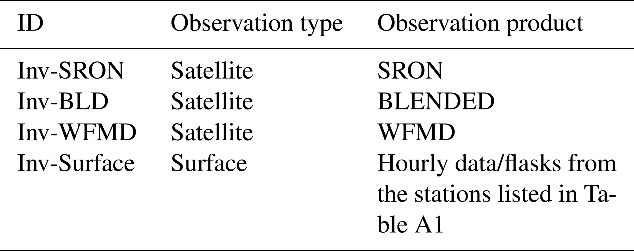
In this study, we perform four 4D-Var inversions assimilating real observations, using the CIF. The CIF is a modular inverse modeling platform developed as a python library (Berchet et al., 2021), designed in the framework of European and international projects. It can drive various data assimilation schemes and can be coupled to various CTMs. Here, the cost function J is minimized using the quasi-newtonian M1QN3 algorithm (Gilbert and Lemaréchal, 1989). The inversion is stopped when the gradient norm reduction exceeds 95 % compared to its initial value. The first three inversions assimilate separately each one of the TROPOMI products. An additional inversion assimilating surface observations (stations listed in Table A1) is performed for evaluation. These four inversions are listed in Table 2.

Table 2 Synthesis of the inversions performed in this study. Results are presented in Sect. 3.3.

2.4.3 Observing System Simulation Experiments

We also explore the capability of the inversion set-up to derive robust emission estimates based on the assimilation of TROPOMI products in a set of Observing System Simulation Experiments (OSSEs). The OSSE approach (Lahoz and Schneider, 2014) makes it possible to evaluate the sensitivity of the inversions to the observation coverage, the observation errors and the differences between products, comparing the results of multiple OSSE scenarios. The structure of an OSSE is described in Fig. 6. The general principle consists of two main parts (Brasseur and Jacob, 2017): first, the sampling of “true” synthetic observations, given a true state defined by the prior emissions and background concentrations. Then, a Monte-Carlo ensemble of inversions with perturbed priors is performed, to evaluate the capability of the observing system to recover the true state of the emission and background estimates.

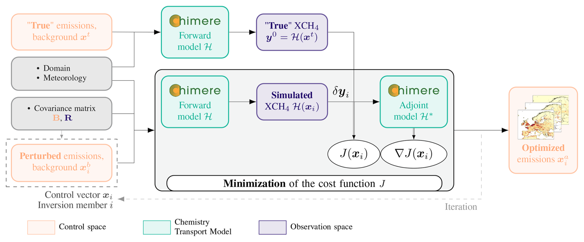
Figure 6 OSSE structure within the CIF. “True” pseudo-observations y⁰ are synthesized from the prior emissions x^t and then assimilated in an ensemble of inversions using perturbed prior fluxes ${\mathit{x}}_i^b$. See http://community-inversion.eu (last access: 22 July 2026).

In more details, a forward run of the CHIMERE CTM produces a “true” 4D concentration field, based on the prior emissions and the prior background concentrations (called x^t). Pseudo-observations y⁰ are sampled from this field following the specifications (date, location, averaging kernels …) of the observation dataset.

The pseudo-observations are assimilated in an ensemble of n=4 inversions using randomly perturbed priors: for each inversion member i, the priors are initially perturbed (called ${\mathit{x}}_i^b$) according to the error statistics provided in B (Sect. 2.4.2):

$$\begin{array}{}\text{(3)}& \forall i\in [\mathrm{1},n],{\mathit{x}}_i^b={\mathit{x}}^{\mathrm{t}}+{\mathit{\eta }}_i,{\mathit{\eta }}_i\sim \mathcal{N}(\mathrm{0},\mathbf{B})\end{array}$$

The metrics used to assess the capability of the system to improve the emission estimates (i.e. to make them closer to the truth) is the relative increment r. It compares the distance to the true initial fluxes x^t of the perturbed prior ${\mathit{x}}_i^b$ and the posterior fluxes ${\mathit{x}}_i^a$, averaged over all the members of the ensemble:

$$\begin{array}{}\text{(4)}& \mathit{r}={\displaystyle \frac{\mathrm{1}}{n}}\sum _i{\mathit{r}}_i={\displaystyle \frac{\mathrm{1}}{n}}\sum _i\left(\left|{\displaystyle \frac{{\mathit{x}}_i^a-{\mathit{x}}^{\mathrm{t}}}{{\mathit{x}}_i^b-{\mathit{x}}^{\mathrm{t}}}}\right|-\mathrm{1}\right)\end{array}$$

The closer r is to −100 %, the more the inversion improves the fluxes. Negative values of r correspond to posterior emissions that are closer to the truth than the prior (thus “better” emissions) while positive values correspond to posterior emissions further from the truth.

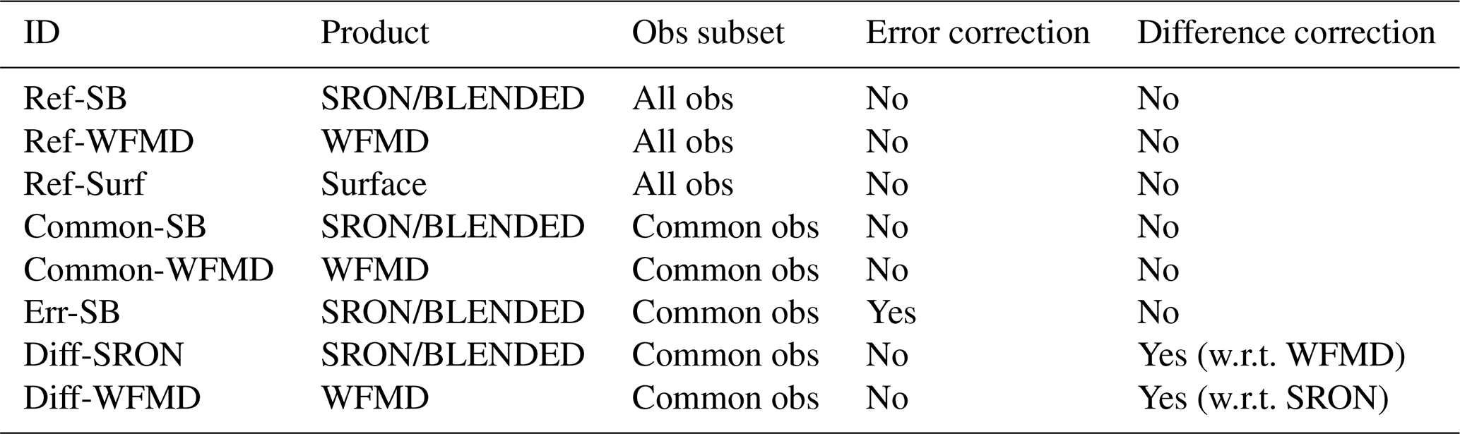
We define 6 OSSE scenarios, listed in Table 3, using different pseudo-observation datasets. To ensure a robust comparison of the scenarios, the seed of the random perturbations is kept constant. It is important to note that since SRON and BLENDED share the same sampling and parameters (errors, vertical profiles), the pseudo-observation datasets are identical. In the following,“SB” scenarios stand for the two products. The 6 scenarios are designed to evaluate the sensitivity of the inversions to multiple parameters:

• 3 OSSEs are performed as reference scenarios using the pseudo-observations of the TROPOMI products: “Ref-SB” for SRON and BLENDED, “Ref-WFMD” for WFMD; a third reference OSSE (“Ref-Surf”) is performed using the pseudo-observations of the surface stations.

• To evaluate the sensitivity to the observation density, 2 OSSEs are carried out assimilating only the pseudo-observations corresponding to the common observations (as described in Sect. 2.1.1). The pseudo-observation datasets differ only by the observation errors and vertical profiles (prior profiles and averaging kernels). These scenarios are referred to as “Common-SB” and “Common-WFMD”.

• To evaluate the sensitivity to observation errors, one scenario is defined using the SRON/BLENDED pseudo-observations dataset, rescaling the errors with Eq. (1). It is called “Err-SB”.

Table 3 Synthesis of all the OSSEs performed in this study. “Common obs” refers to the restriction to observations common to the 3 products, as described in Sect. 2.1.3. The “error correction” corresponds to the application of Eq. (1) to the errors of SRON/BLENDED.

To evaluate the impact of the differences between products, we carry out two more inversions assimilating pseudo-observations. The method differs from previous OSSEs: in this case, synthetic observations are sampled and biased with the difference between products:

• The difference WFMD-SRON (computed over the common observations) is averaged over 0.5° × 0.5° pixels and 1 h-long periods, and added to the corresponding SRON pseudo-observations. The same correction is applied to WFMD pseudo-observations with respect to SRON-WFMD difference. To evaluate the impact of the inter-product difference on the posterior increments, each “corrected” data set is assimilated (priors are not perturbed), the inversions are called “Diff-SRON” and “Diff-WFMD”.

3 Results

3.1 Drivers of the differences in the XCH₄ observed distributions

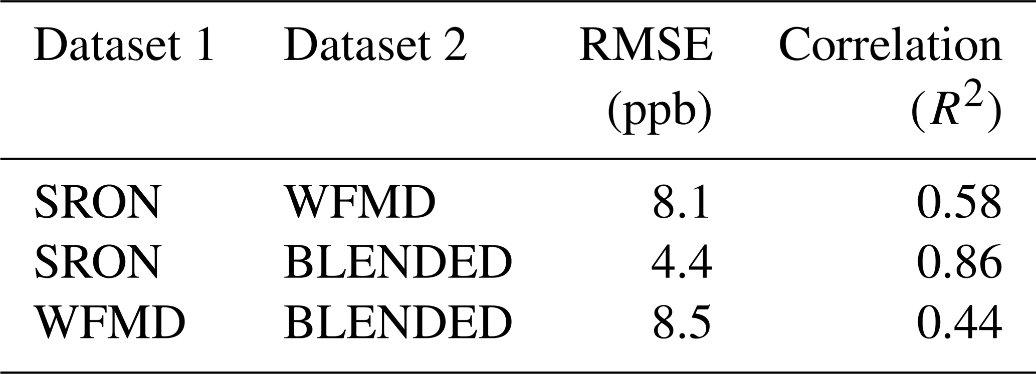
To better understand the inter-product differences related to atmospheric, instrumental and algorithmic variables, we adopt the method of Balasus et al. (2023): we train a ML model to predict the ΔXCH₄ differences between observed values, for each pairwise combination of products, using retrieval parameters as input features. Ten features are included: surface altitude and roughness, SWIR surface albedo, fluorescence, the aerosol size parameter, the SWIR aerosol optical thickness (AOT), the a priori XCH₄ total column and the across-track pixel index, which are retrieved from the SRON product, and the observation errors of the two products for which ΔXCH₄ is predicted. The across-track pixel index provides information about the relative position of the pixel in the swath of the satellite, therefore it is related to the so-called “striping” effect – a systematic artifact observed in TROPOMI CO, H₂O $/$ HDO, and XCH₄ products (Borsdorff et al., 2019). This effect consists in differences of XCH₄ measurements across consecutive parallel strips. The 3 432 335 observations shared across the three products (dataset described in Sect. 2.1.1) are randomly split into a training dataset (90 % of the observations) and a validation dataset (10 % of the observations). We search for the best-performing model between three ML algorithms that rely on decision trees: Random Forest, XGBoost and Light Gradient-Boosting Machine (LightGBM). Random Forest builds an ensemble of decision trees by combining bootstrap sampling and feature randomization, and produces predictions through averaging across the forest (Breiman, 2001). XGBoost and LightGBM apply gradient-boosted decision trees, a method where sequentially trained decision trees minimize a loss function by correcting the residual errors of the previous trees, thereby iteratively enhancing accuracy. XGBoost employs advanced regularization (L1 and L2 penalties) and parallelized tree construction (Chen and Guestrin, 2016). In contrast, LightGBM adopts a histogram-based learning approach and exclusive feature bundling (Ke et al., 2017).

In all cases, LightGBM outperforms the other models, while Random Forest systematically shows the lowest performances. Table 4 presents the validation results for the LightGBM model, which was ultimately chosen for further analyses. The predictive performances are consistent with the results of Balasus et al. (2023) for the prediction of the XCH₄ differences between TROPOMI and GOSAT, in terms of RMSE (Root Mean Square Error) and correlation (RMSE =12.4 ppb, R²=0.53).

Table 4 Validation results of predicted ΔXCH₄ for each combination of products, with the best-performing model (Light GBM).

Beyond its predictive performances, the trained model provides insights into the most important features – that is, the features that contribute most to the prediction of ΔXCH₄. We conduct a study using SHapley Additive exPlanations (SHAP) on the predictions of the model, following Balasus et al. (2023). This approach partitions an individual prediction into contributions attributed to each feature, quantified as SHAP values (in ppb). The sum of all SHAP values for a given prediction corresponds to the difference between that prediction and the mean prediction across the entire dataset. The input features can then be ranked using the average absolute SHAP values, for each product pair comparison (Fig. 7). Our findings align closely with those of Balasus et al. (2023): the most impacting features on the differences between satellite products are the across-track pixel index (thus striping patterns), aerosols and SWIR albedo. Calculating the mean ratio between the absolute SHAP value and the sum of the absolute SHAP values of all the features, the contributions are between 20 % and 29 % of the difference for aerosols, 13 % to 19 % for striping patterns, and 13 % to 14 % for albedo. The observation errors also seem to impact the prediction. Features related to aerosols are the SWIR aerosol optical thickness (AOT) and the aerosol size parameter, which are strongly anti-correlated ($R^{\mathrm{2}}=-\mathrm{0.82}$). Since the SHAP analysis does not fully resolve correlations between variables, we aggregated the contributions of these two features into a single combined SHAP value, hereafter called ”aerosols”, to preserve interpretability.

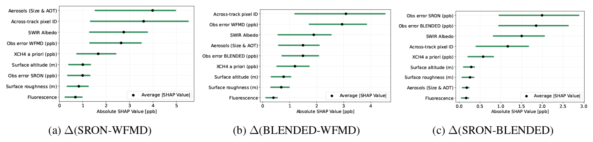
Figure 7 Contributions of the individual features to the ΔXCH₄ predictions between pairs of TROPOMI products. The 9 most impacting predictors are ranked in order of importance. The contribution of a feature is defined as the average of absolute SHAP values, with the green bar showing the interquartile range.

We focus on the impact of albedo, aerosols and striping patterns on the XCH₄ differences between products: Fig. 8 illustrates the variations in observed XCH₄ as functions of SWIR albedo, aerosol size parameter, and across-track pixel index. The albedo and aerosol parameters are retrieved with the SRON algorithm: it is important to mention that the accuracy of these retrievals is not clearly known.

• Albedo. XCH₄ are influenced by surface reflectance, particularly in scenes with low SWIR albedo (e.g., snow, water bodies) or high SWIR albedo (sandy areas). In all the products, the albedo dependence is corrected based on a polynomial fit to the surface reflectance spectrum in the 2.3 µm spectral range. The polynomial degree was increased from 2 to 3 in recent updates of the products (Lorente et al., 2023; Schneising et al., 2023). Despite these adjustments, the products show different variations with SWIR albedo, as illustrated in Fig. 8a. BLENDED and WFMD have a consistent low dependency on the albedo in the range of values between 0.05 and 0.5, where the density of observations is high. However, there is an offset of approximately 10 ppb, which decreases at high albedo values. SRON XCH₄ observations show more variations: they are close to those of WFMD at low albedo values, but lower than the other two products for high albedos.

• Aerosols. The effect of aerosols on methane retrievals is well-known: scattering by aerosol particles modifies the light path and induces errors that can compromise the accuracy of the retrieval (Butz et al., 2012). It depends on aerosol amount, type and size distribution. The latter is characterized by the aerosol size parameter α, which is the negative exponent of the power law of the aerosol size distribution $n\left(r\right)\propto r^{-\mathit{\alpha }}$, with r the particle radius: the higher α is, the more n(r) is shifted towards small particle sizes. It is simultaneously inferred and corrected during the XCH₄ retrieval process of SRON (Hasekamp et al., 2022), yet it still strongly impacts XCH₄ observations. TROPOMI SRON data is biased low relative to GOSAT for low values of α, indicating large particles (Balasus et al., 2023), as confirmed by Fig. 8b. The correction applied in the BLENDED product makes its sensitivity to α closer to the one of WFMD, in comparison to SRON. Still, the three products show different behaviors and seem to be consistent only for α>4.4, which corresponds to a small part of the observations.

• Striping patterns. Without dedicated destriping, stripes in the flight direction are visible in the TROPOMI XCH₄ data, likely due to variations in the offsets and gains of detector pixels. While the across-track pixel index is included in the calibration process of the WFMD retrieval, residual vertical stripes persist in the data (Schneising et al., 2023). The latest WFMD product (v1.8) mitigates this effect using a wavelet–Fourier decomposition and filtering (Schneising et al., 2023). Indeed, Fig. 8c) depicts the higher sensitivity of the SRON product to this effect. The correction with respect to GOSAT applied in the BLENDED product yields slightly lower sensitivity regarding the striping effect (Fig. 8c). A recent method based on a double moving median smoothing along both the flight and cross-track directions resulted in promising enhancements in striping correction for the operational SRON product. It is implemented into newer versions of the product (Borsdorff et al., 2024), but older orbits have not been reprocessed. Future uses of the SRON destriped data should improve the consistency of XCH₄ observations with the other products.

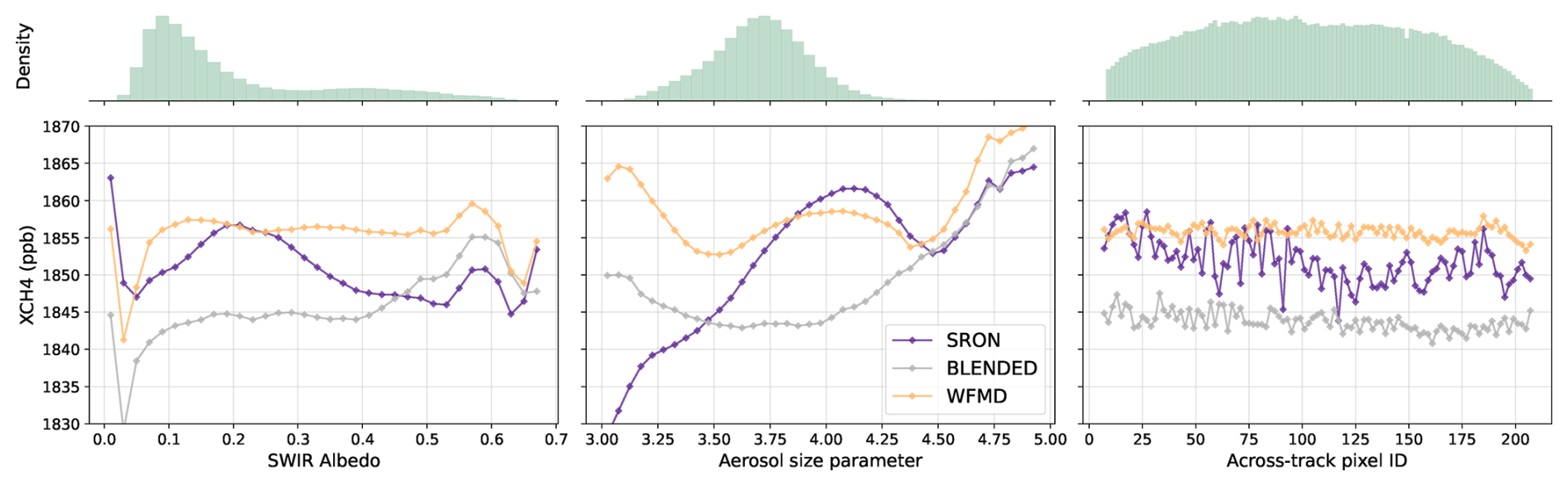
Figure 8 Observed XCH₄ total column vs. SWIR albedo, aerosol size parameter and across-track pixel index. These three parameters are retrieved with SRON algorithm. The histogram depicts the density of common observations with respect to the corresponding variable.

3.2 Comparison between observed and simulated CH₄ total columns

The differences in the simulated XCH₄ between the three TROPOMI products are linked to the differences in observation coverage and in the vertical profiles that are necessary to compute their simulated equivalents, as described in Sect. 2.1.1. The mean biases (MBs) of the difference $\mathrm{\Delta }{\text{XCH}}_{\mathrm{4}}^{\mathrm{os}}={\text{XCH}}_{\mathrm{4}}^{\mathrm{obs}}-{\text{XCH}}_{\mathrm{4}}^{\mathrm{sim}}$ with the prior inputs are approximately 6.7, -0.4 and 4.4 ppb and the RMSEs 18.2, 13.6 and 15.4 ppb respectively for SRON, BLENDED and WFMD (top row of Fig. 9). BLENDED demonstrates both a smaller bias and a lower RMSE between observations and simulations, in comparison to SRON and WFMD.

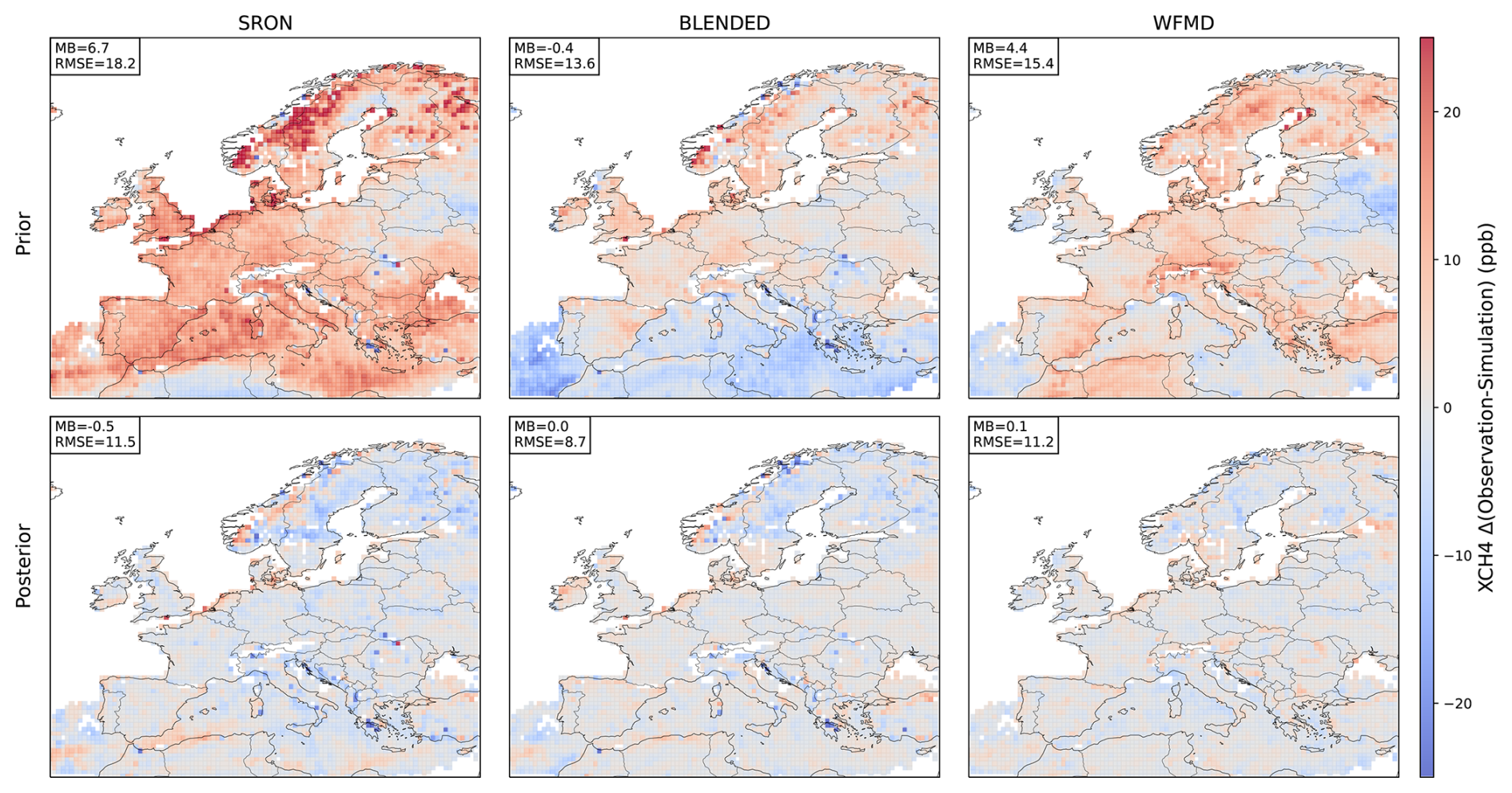
Figure 9 Annual average difference between TROPOMI observations and their CHIMERE simulated equivalents, using prior emissions (first row) and posterior emissions (second row). MB is the mean bias and RMSE the root mean square error, in ppb. Only the cells with at least 50 observations in 2019 are shown.

When the analysis is restricted to the subset of matching observations across the three datasets, the RMSE decreases for all products, to respective values of 17.4, 13.1 and 13.0 ppb. This improvement indicates that the application of combined filters, which more rigorously select high-quality data, reduces the gap between observed and simulated concentrations.

The spatial distributions of the differences between observed and simulated concentrations $\mathrm{\Delta }{\text{XCH}}_{\mathrm{4}}^{\mathrm{os}}$ (top row of Fig. 9) reveal common patterns but also notable discrepancies across the three TROPOMI products. For all products, simulated XCH₄ are overall lower than observations over land. SRON has the highest difference between observed and simulated XCH₄ over land, especially in Western Europe. Over the sea, the simulations behave very differently across products: SRON shows a positive difference, while it is negative for BLENDED and close to 0 for WFMD. The difference between SRON and BLENDED is consistent with the systematic downward correction over the ocean depicted in Balasus et al. (2023).

Seasonal variations in the $\mathrm{\Delta }{\text{XCH}}_{\mathrm{4}}^{\mathrm{os}}$ are generally consistent across the three products (Fig. D3). $\mathrm{\Delta }{\text{XCH}}_{\mathrm{4}}^{\mathrm{os}}$ are high during the first half of 2019 and decrease in the second half of the year; the RMSE decreases by more than 20 % from winter (i.e. January to March) to summer (i.e July to September) for all products, though this overall reduction masks spatial heterogeneities. Scandinavia stands out as a region with marked discrepancies between observations and simulations: for SRON, $\mathrm{\Delta }{\text{XCH}}_{\mathrm{4}}^{\mathrm{os}}$ reaches high positive values from April to June and is negative between October and December (Fig. D3). The seasonal variations are consistent across the three products in this region, though with lower amplitude for BLENDED and WFMD. The differences in behaviour among products in regions like North Africa and Scandinavia highlight the influence of surface albedo and aerosols on observations. This effect predominantly affects observed concentrations, as simulated equivalents exhibit limited dependence on the parameters identified in Sect. 3.1 (not shown).

Overall, simulated concentrations are underestimated compared to observations over land across all TROPOMI products, with BLENDED providing the closest match. The residual (difference between the observed XCH₄ and the posterior simulations) is reduced after the inversion: the mean biases are decreased from the prior to the posterior simulation by approximately 93 %, 95 % and 99 % for SRON, BLENDED and WFMD respectively (bottom row of Fig. 9). Similarly, the RMSE decreases by 37 %, 36 %, and 28 % for these products. The correlation coefficient between observed and simulated XCH₄ is also increased (Fig. S3).

3.3 TROPOMI-derived CH₄ emissions : spatial and temporal distributions, annual budgets

Inversions are performed using the method detailed in Sect. 2.4.2. The three inversions assimilating each TROPOMI product, as well as the additional inversion using surface data for evaluation, are listed in Table 2. Figure 10 shows the corrections to the prior CH₄ emissions from these inversions, referred to as increments, both at the grid-cell and national resolutions. We remind the reader that the purpose of the inversion is not to attribute emissions to specific point sources or to individual sectors within a grid cell, but to solve for the aggregation of strong localized sources and diffuse sources over large scales.

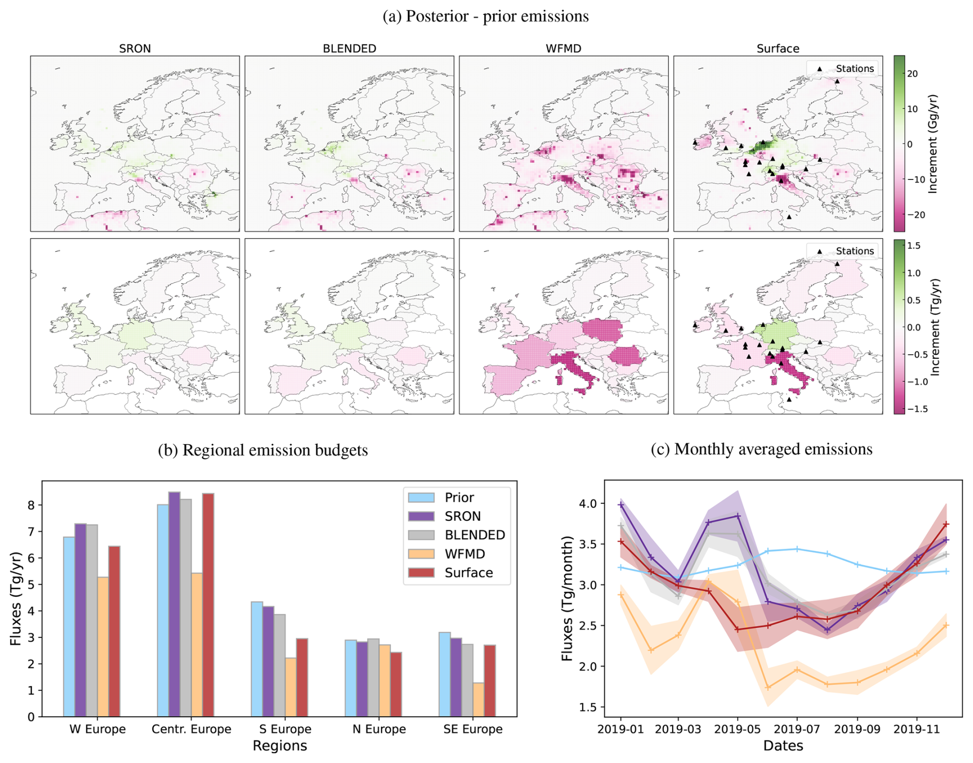
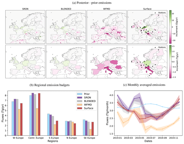
Figure 10 (a) Spatial distributions of the increments to the prior CH₄ emissions from the inversions, in Gg yr⁻¹ at the grid-cell resolution (first row) and in Tg yr⁻¹ at the national resolution (second row). (b) Total emissions for the regions described in Table B1, in Tg yr⁻¹. (c) Monthly variations of the CH₄ emissions in the domain in 2019, in Tg per month. The shaded areas show the standard deviation within each month.

The increments differ among the inversions (Fig. 10a), and these differences result in large differences in the total CH₄ emission budgets for 2019, for the regions and the corresponding countries listed in Table B1. While the prior total emissions of 25.2 TgCH₄ yr⁻¹ are increased by 2 % for the SRON (25.7 Tg yr⁻¹) inversion, they are reduced by respectively 1 %, 9 % and 33 % for the BLENDED (25.0 Tg yr⁻¹), surface-based (23.0 Tg yr⁻¹) and WFMD (16.9 Tg yr⁻¹) inversions. The detailed comparison of prior and posterior emissions per country is shown in Table S1 in the Supplement. While some regions exhibit consistent corrections across all three TROPOMI inversions (e.g. in Northern Africa, Italy or Romania), the magnitude of increments is generally larger in the WFMD-based inversion in comparison to SRON and BLENDED, consistently with the OSSEs of Sect. 3.4. Aggregation at the national scale mitigates some of these inconsistencies but reveals high differences in countries such as the Netherlands, Germany, France, and Poland (Fig. 10a). SRON and BLENDED provide similar corrections to the prior CH₄ emissions in most countries, except Poland and Turkey, but they differ from WFMD particularly in Western and Central Europe (Fig. S4).

It is important to note that the surface-based inversion is influenced by the spatial distribution of the stations: regions with dense station coverage, such as Western Europe (8 stations), are well constrained, whereas regions with sparse coverage, like the Baltic states, Spain and Portugal show little correction of the prior fluxes. Scandinavia is poorly constrained in all satellite inversions, whereas small increments appear in Northern Finland in the surface-based inversion due to the presence of the Pallas station. Despite these limitations, the comparison of satellite-based inversions with the surface-based inversion shows some consistency: surface-based increments agree well with WFMD corrections over the Paris area and Italy, and with SRON and BLENDED corrections over the Netherlands and Switzerland. However, the surface-based inversion is not consistently closer to one satellite-based inversion than to another, as indicated by the R² correlation coefficients between surface-based increments and satellite-based increments (0.24 for SRON, 0.34 for BLENDED, and 0.37 for WFMD).

The temporal variations of CH₄ emissions is shown in Fig. 10c. Satellite-based inversions exhibit similar temporal patterns, including high emissions during December and January, a peak in April or May, and lower emissions over the summer months. Despite these similarities, WFMD-based emissions are systematically lower than those from SRON and BLENDED, contributing to the lower annual total mentioned earlier. The monthly corrections to prior CH₄ emissions differ between satellite-based and surface-based inversions. For example, the peak of emissions during spring detected in the satellite inversions is not found in the surface-based inversion (Fig. 10c). This peak is due to positive corrections in Western and Central Europe across all satellite-based inversions. This period coincides with a slight decline in observed XCH₄ (Fig. 2a), and an increase (for the month of April) in the lateral boundary conditions (Fig. D4). Yet, the origin of this emission peak has not been clarified.

Both TROPOMI-based and surface-based inversions capture the summer emission minimum, which contrasts with the prior emissions, where the minimum occurs in autumn and winter. This unexpected seasonal cycle, already identified in Pison et al. (2021), seems to be related to CHIMERE transport modeling since it did not occur when using other models like FLEXPART. It is likely due to a misrepresentation of the atmospheric transport or poor representation of the seasonality of boundary conditions (Pison et al., 2021). Other transport model errors (miscalculation of the tropopause height, mesoscale transport errors) can impact the calculation of simulated XCH₄ (Saad et al., 2014), thus biasing the results of the inversions. However, a dedicated study would go beyond the scope of this article, and we do not address the impact of model errors and how they interact with the retrieval biases.

The nearly identical emission increments for SRON and BLENDED (Fig. 10) show that corrections for albedo and aerosol related biases in BLENDED do not lead to any significant differences in the derived emissions. Indeed, the logic for BLENDED is to solve these biases of the SRON XCH₄ retrievals using GOSAT retrievals. Therefore, this suggests that potential albedo and aerosol related biases (depicted in Sect. 3.1) are not significantly impacting the derived CH₄ emissions in Europe, within the scope of our study.

Figures S5 and S6 show scatter plots of posterior emissions against prior emissions, at the pixel and weekly scale (Fig. S5) and aggregated at the monthly and national scale (Fig. S6). The previously mentioned differences between the distributions of posterior emissions are clearly observed at the pixel scale. The variability decreases when aggregating the fluxes, yet remains substantial across the posteriors of the four inversions. It highlights the limits of the current use of the TROPOMI products to build national CH₄ budgets and attribute emissions. Also, negative emissions can be seen for the posteriors in Fig. S5: the negative posterior emissions that do not correspond to sinks in the prior correspond to a low number of control vector values (1.0 %, 0.2 %, 4.9 % and 2.3 % of the pixels respectively for SRON, BLENDED, WFMD and Surface). To avoid such negative emissions, log-normal distributions for the emissions could be used (instead of normal distirbutions) to ensure positive fluxes, while optimizing sinks separately (Bergamaschi et al., 2022; Hancock et al., 2025). Another option would be to filter out the negative values as described in Zheng et al. (2026), but the truncation of gaussian distributions would require accurate statistical sampling of the new estimate of the analysis after the truncation (Lauvernet et al., 2009). We choose not to filter negative emissions, to remain in the framework of Bayesian inversions.

To complete the analysis of posterior emission differences, a further comparison of the increments in the background components of the control vector (as defined in Sect. 2.4.2) reveals that, while the increments exhibit some similar patterns, they overall differ for the three TROPOMI products. The average background total columns are increased in average by 3.5, 1.4 and 2.1 ppb for respectively SRON, BLENDED and WFMD (Fig. D5). The increments in the stratosphere share common patterns of positive increments over the Mediterranean basin, but with differing magnitudes: they are stronger for SRON and WFMD than for BLENDED. The lateral boundary increments are mainly positive over the western limit for SRON, BLENDED and the surface-based inversion, with the higher values for SRON. WFMD shows a different pattern for the increments of the lateral boundary conditions, with an increase of the background at the southern border of the domain. The time variations of the increments are overall consistent between products, only the magnitude changes across the inversions (Fig. D4).

For BLENDED, the close agreement between observed and simulated XCH₄ leads to a lower magnitude of both flux and background increments in comparison to other inversions. SRON has higher background increments in average than WFMD, consistently with the higher difference of observed and simulated XCH₄ showed in Fig. 9. However, for SRON the emissions are not pulled down as strongly as for WFMD. For this latter product, the background and flux increments do not seem to be anti-correlated, which could have been expected as the differences between the observations and the prior simulations were not that high and the fluxes strongly decreased through the inversion. Therefore, the strong negative increments on the Inv-WFMD fluxes result from a complex balance between the local gradients of the increments on the background and on the fluxes: the system could have difficulty separating both when using the WFMD observations. The differences between products detailed in Sects. 2.1.3, 3.1 and 3.2 could push the system towards different splits between background and emission optimization.

3.4 Separation of the causes of differences through OSSEs

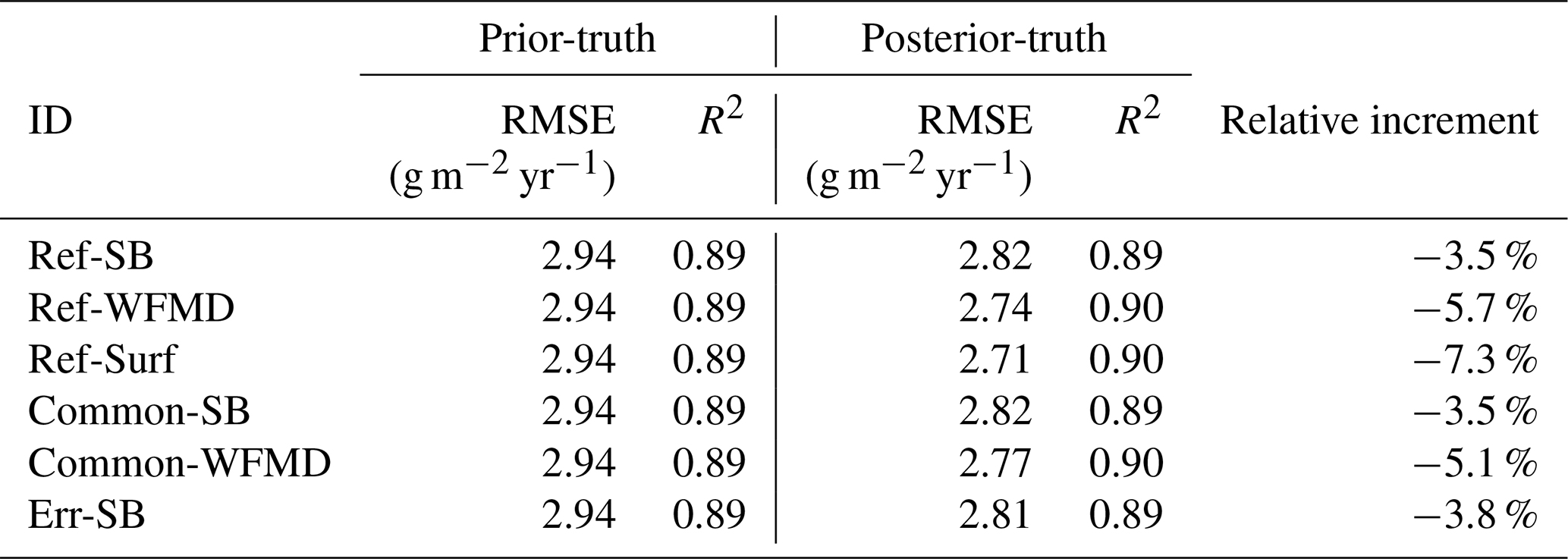
Previous sections highlighted the differences in the products, in the observed and simulated XCH₄ distributions and in the results of inversions. To deepen the understanding of the differences of inversion outputs, we compare here the capacity of the system to improve emission estimates through the inversion, for the three products. As described in Sect. 2.4.3, OSSEs are a relevant tool to evaluate this capability, to perform sensitivity tests on the inversion procedure and to discriminate between the causes of the differences in the fluxes derived from various inversions. Following the method and notations of Sect. 2.4.3, the “prior” refers to the perturbed prior x^b, while the “truth” corresponds to the unperturbed prior x^t. The performances of an OSSE are assessed using the relative increment, as defined in Eq. (4): the closer to −100 % r is, the closer the posterior fluxes are to the truth (in comparison to the prior). This metric is calculated only over land to avoid averaging effects caused by weak fluxes over the sea. Table 5 shows the relative increment for the first six OSSE configurations (described in Table 3), as well as the RMSE and R² coefficient between the perturbed prior fluxes (averaged over all the members) and the true fluxes, and between the posterior and the true fluxes.

Table 5 Evaluation results of 6 OSSE configurations. “Prior” refers to the perturbed prior fluxes, “Truth” to the unperturbed prior fluxes and “Posterior” to the optimized fluxes after the inversion. All the fluxes (thus the RMSE) are in units of gCH₄ m⁻² yr⁻¹. The prior and posterior have been averaged over all samples of the OSSE. The relative increment is calculated only over land. Diff-SRON and Diff-WFMD are not included since prior emissions were not perturbed. Scenario IDs refer to Table 3.

3.4.1 Reference scenarios

The Ref-SB and Ref-WFMD OSSEs demonstrate a consistent capacity to constrain emission estimates. Despite the relatively low values of r (in comparison to the aim of −100 %), we focus on the relative differences of r between scenarios. The temporal (Fig. 11a) and spatial (Fig. 11b) variations of the relative increments are consistent across the three products. Monthly variations smooth the noisier weekly variations in Fig. 11a, but relative differences between scenarios are conserved. WFMD presents the highest performance, with a mean relative increment of −5.7 %, in comparison to −3.5 % for SRON/BLENDED, and a larger reduction in RMSE (Table 5). This product thus presents a higher constraint capacity in comparison to SRON and BLENDED.

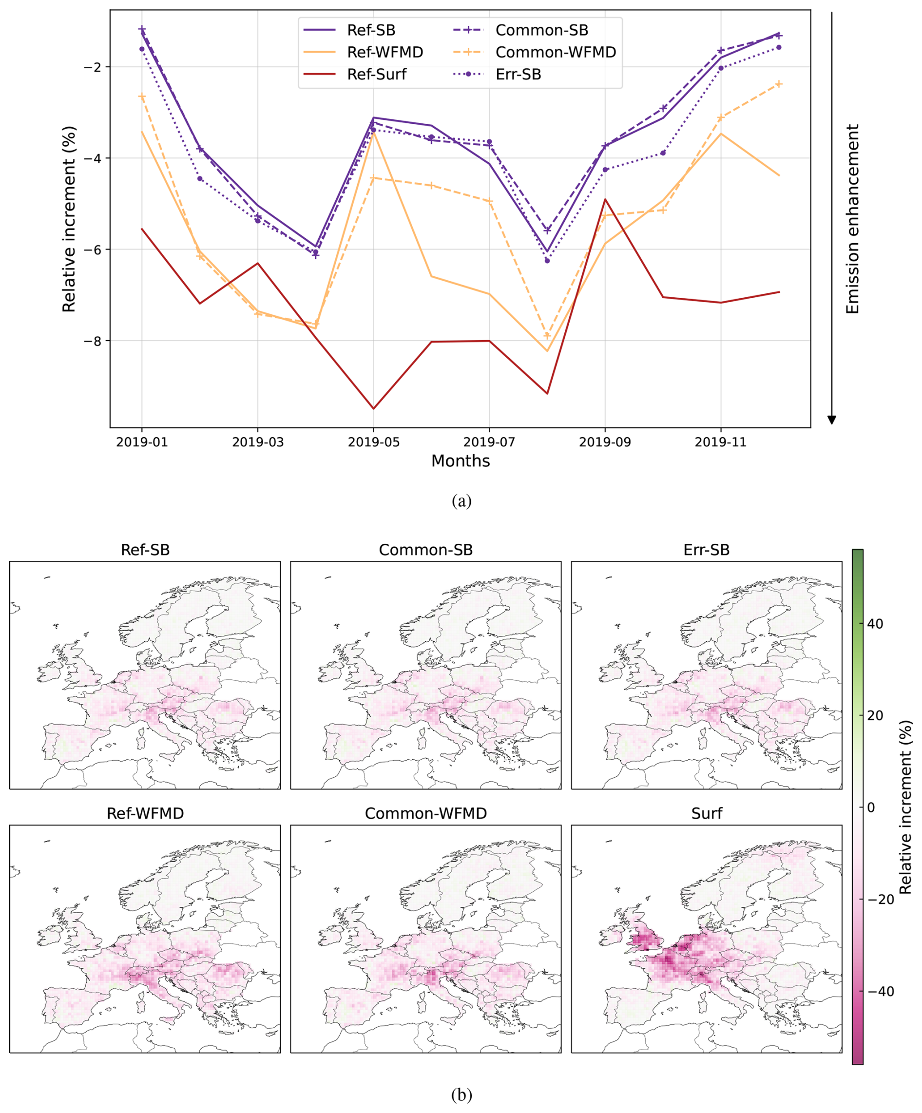
Figure 11 (a) Average monthly relative increment (%) over 2019 and (b) maps of relative increment (%), for the different OSSE scenarios. These scenarios are described in Table 3. The lower the relative increment, the more posterior fluxes are closer to the truth (Eq. 4). The regions are described in Table B1.

The prior temporal variations of emissions remain largely preserved through the assimilation of pseudo-observations. Consequently, the posterior time variations align closely with those of the unperturbed prior. However, the relative increment varies over the year (Fig. 11a). These variations are partially influenced by the observational density, with lower r (i.e. closer to −100 %) in summer, coinciding with an abundance of high-quality measurements, and higher (i.e. further from −100 %) values in January and December, when coverage decreases due to cloud filtering. A small $\left|r\right|$ is also seen in May 2019, likely caused by the low number of observations (Fig. 1b).

Regions with sparse observational coverage generally exhibit worse (i.e. closer to 0) relative increments. In particular, the system fails to improve emission estimates in Scandinavia across all three configurations (Fig. 11b). This limitation is directly related to the sparse observation density in this region (Fig. 1b), with nearly no observations available during winter. Due to a sparse observation density, the system also performs poorly in the United Kingdom (Fig. 11b), contributing to the poor mean relative increment over Western Europe.

The system manages to make the posterior emissions closer to the truth in areas with high fluxes (northern Italy, Benelux, Romania) while struggling in areas with weaker signals, like Latvia and southern France (Fig. 11b). This is linked to the prior error covariance B being proportional to the emissions (see Sect. 2.4.1), which limits the ability of the inversion to recover diffuse sources with low signal-to-noise ratios, as previously noted by Yu et al. (2021).

These reference OSSE scenarios demonstrate the capability of all TROPOMI products to bring emission posteriors closer to the truth compared to the perturbed priors. The Ref-Surf scenario provides a better overall enhancement, with an average relative increment of −7.31 %. However, this better result on average masks a high spatial heterogeneity: the relative increments are indeed very good in Western Europe and Central Europe where a number of stations are located, but fail to provide enhancements in regions with no stations, such as Spain or Romania (Fig. 11b). As expected, the wider coverage of satellite observations provides the advantage of constraining the emissions on a wider area, even if there are no surface stations.

The OSSEs can also be used to estimate the uncertainty reduction (independent of the control vector) for the inversions, computing the ratio between the standard deviation of priors and the one of posterior emissions across the ensemble samples. For the total budgets, it is estimated to 78 % reduction for SRON and BLENDED, 74 % for WFMD and 51 % for surface stations. However, we do not use them for evaluating the uncertainties of our budget estimates in Sect. 3.3, because of 1) the small size of the ensemble (4 samples) and 2) the lack of proper uncertainty estimation for the prior (not provided with the emission inventories). The estimation of the uncertainty requires a deeper analysis of the propagation of errors through the system: observation errors (Zheng et al., 2026) as well as model errors due to the prior emissions and the transport (Lu et al., 2025a).

3.4.2 Drivers of the differences of increments

Observation density

The relationship between observation density and constraint potential is explored through the Common-SB and Common-WFMD OSSEs. As expected, the relative increments are slightly closer to zero as observation density decreases (Table 5). The average difference in comparison to the reference scenario is very low (less than 0.01 gCH₄ m⁻² yr⁻¹ in RMSE) for SRON/BLENDED, with 73 % of the observations kept in Common-SB, but slightly higher (0.03 gCH₄ m⁻² yr⁻¹ in RMSE) for WFMD because the difference in observation density is larger (45 % of observations kept). The time series of Ref and Common scenarios in Fig. 11a illustrate that the relative increment is overall slightly deteriorated, yet not systematically, as the number of observations decreases. The observation density is thus a driver of the potential for constraining emissions through the inversion. However it only partially explains the differences of performance between the products, since Common-WFMD results in lower relative increments than Common-SB: even with the same number of observations, WFMD seems to show a better capability to bring emission closer to the truth. The key differences between these scenarios lie in the uncertainties associated with the measurements and the vertical parameters (such as pressure levels, AKs, and prior profiles) used to compute the satellite equivalents.

Error rescaling

The linear rescaling of the error associated with individual observations, described in Eq. (1), increases these individual errors in the dataset of pseudo-observations. The comparison of Err-SB scenario to Common-SB shows a slight improvement of the emissions for all months (Fig. 11a) and all regions (Fig. 11b), when rescaling these errors. The spatial distributions are similar, as shown in Fig. 11b, but with a slightly larger amplitude for Err-SB.

The Err-SB scenario is the closest SRON/BLENDED scenario to WFMD ones in terms of relative increment (Fig. 11). The Err-SB and Common-WFMD, which share similar features in terms of coverage and errors, have the highest consistency between SRON/BLENDED and WFMD OSSEs, highlighting these features as drivers of the differences in inversion results. The remaining differences are due to the vertical parameters (pressure levels, averaging kernels, and prior profiles).

Rescaling the observation error results in an enhancement of the emissions. This counterintuitive effect is likely due to overfitting and complex indirect effects within the inversion: because of the large number of observations and the low individual observation errors, the system could struggle to overfit the observations, thus degrading the performances. At the 0.5° resolution, several observations constrain each component of the control vector, leading to overfitting of some observations if the errors are small. This effect would be mitigated in the Err-SB scenario, leading to better (i.e. more negative) r. Still, this effect is limited (r varies by a few 0.1 %) in comparison to the differences of r between products.

SRON-WFMD XCH₄ difference

The scenarios Diff-SRON and Diff-WFMD provide insights into how the bias between products impacts the retrieved flux distribution. In this section, we do not focus anymore on the relative increment (fluxes are not perturbed in the Diff scenarios), but on the increments derived from the assimilation of the biased observations.

As expected, the opposite biases result in overall opposite increments. The assimilation of biased observations leads to an increase in total emissions for SRON (from 25.2 to 25.3 Tg yr⁻¹) and a decrease for WFMD (from 25.2 to 24.3 Tg yr⁻¹), consistently with the average positive difference between WFMD and SRON. However, these small differences in total emissions are the sum of large spatial variations, as shown in Fig. 12b. The maps highlight the contribution of the WFMD-SRON difference to the SRON increments, with negative increments in Western Europe (UK, Ireland, eastern Spain), southern Italy and Austria/Czech Republic, particularly over mountainous regions like the Pyrenees and the High Tatras in Central Europe. Positive contributions are observed across most of Eastern Europe, Benelux/Germany, central Italy and the Alps. While these contributions should be closely related to the difference of XCH₄ columns, shown in Fig. 12a, no clear correlation emerges between the bias in the concentrations and the corrections in the emissions: the average SRON-WFMD difference is generally negative and smooth, in contrast to the localized, strong increments in the emissions.

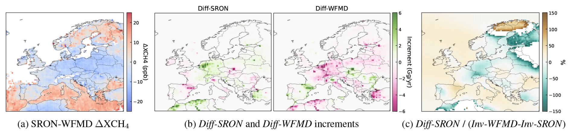
Figure 12 Spatial averages of (a) the XCH₄ difference SRON-WFMD (in ppb), (b) the increments of the Diff-SRON and Diff-WFMD OSSEs (in Gg yr⁻¹) and (c) of the ratio between the increments of Diff-SRON by the difference of increments between inversions Inv-WFMD and Inv-SRON (in %). For the last map (c), pixels with ratios above 150 % (corresponding to very close increments in Inv-WFMD and Inv-SRON) were filtered out.

Yet, these two OSSE scenarios help clarify some of the patterns observed in inversions with real data. The increments of Diff-SRON (biased by the WFMD-SRON difference) and the difference of increments between inversions Inv-WFMD and Inv-SRON descrived in Sect. 3.3 are compared in Fig. 12c. The ratio between these two quantities show that the differences in the inversion increments can be partially explained by the difference SRON-WFMD over the sea, in Western Europe or in Romania. However, blue areas in Central Europe and Eastern Europe show opposite variations, meaning that the OSSE increments are not sufficient to explain the increments in the inversions with real data. This suggests that while XCH₄ differences provide some explanation, they do not fully account for the inversion outputs. In inversions, the CAMS background is also optimized and transport is not assumed perfect, contrary to OSSEs: it makes the tracing of the main factors impacting the increments on fluxes more complex.

3.5 Evaluation against independent surface measurements

Finally, we evaluate the TROPOMI-based inversions described in Sect. 3.3 with independent surface data. To evaluate the consistency of satellite-based and surface-based perspectives, we compare the posterior simulated concentrations to independent methane observations from the surface stations listed in Table A1. The mean biases, RMSEs and correlation coefficients are summarized in Table 6.

Table 6 Comparison of the mean bias (MB), RMSE and R² between independent surface measurements and the simulated concentrations using respectively the prior emissions and the posterior emissions from the four inversions. The high RMSE (in comparison to the MB) highlights the variability of observation/simulation comparison for surface measurements.

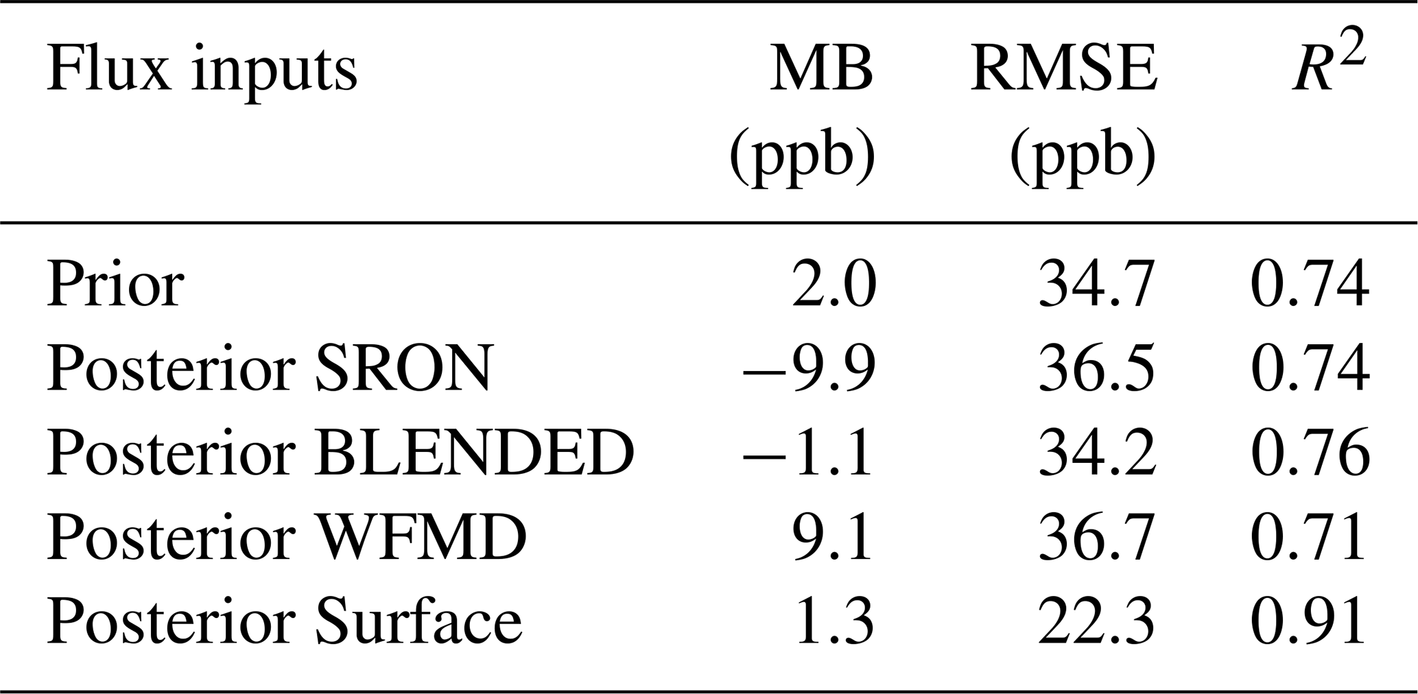
Considering all surface measurements, the average difference between XCH₄ observations and the prior simulations is 2.0 ppb. It is closer to 0 than the average difference between XCH₄ observations and the posterior simulations for SRON and WFMD (respectively −9.9 and 9.1 ppb). For these two simulations, the RMSE is also higher than for the prior simulation. However, the absolute mean bias and RMSE are closer to 0 for BLENDED posterior simulations, in comparison to the prior: this product is more consistent with surface station measurements than the other two. In Inv-Surface, the differences are decreased for almost all stations, as expected.

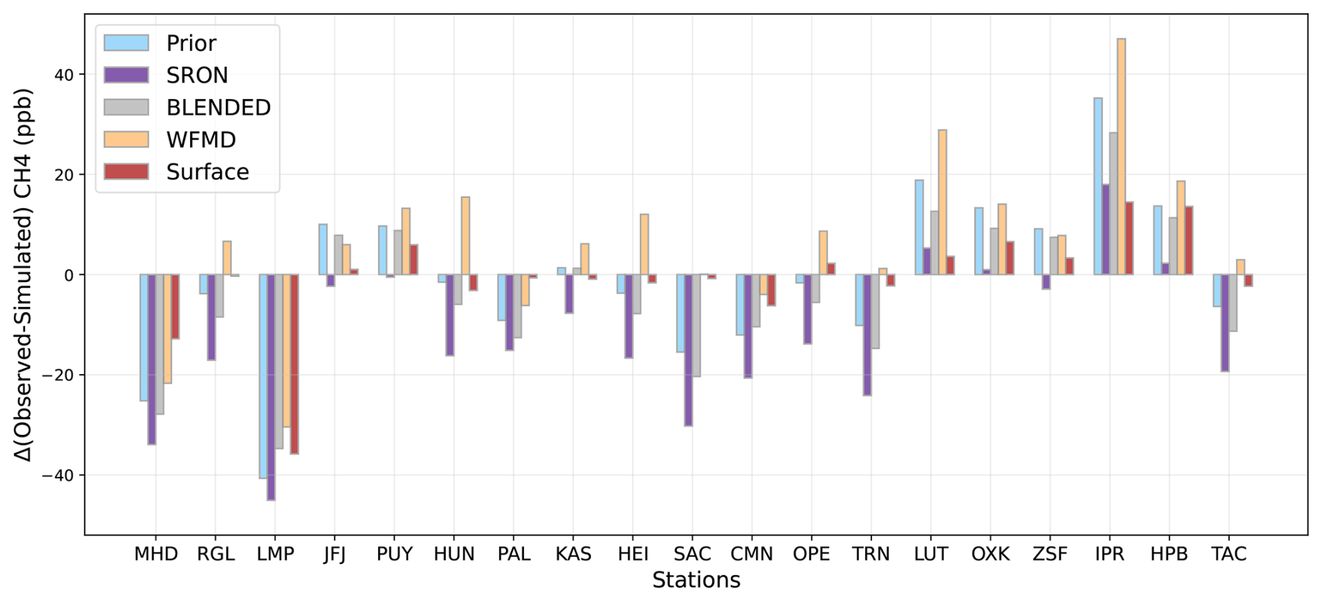
Figure 13 Differences between independent surface measurements and the simulations (in ppb) using the prior emissions and the posterior emissions from the SRON, BLENDED and WFMD and Surface-based inversions, for the stations described in Table A1.

The overall statistics mask a heterogeneous distribution of differences across individual stations. The corrections to the prior CH₄ emissions derived from satellite-based inversions improve the fit with surface measurements for about half of the stations: 37 % for SRON, 53 % for BLENDED, 47 % for WFMD (Fig. 13). For SRON and BLENDED posterior simulations, the difference is deteriorated at most stations with simulated equivalents generally higher than the observations, especially over the UK, Ireland and France (MHD, RGL, TAC, SAC, OPE, Fig. D2). It is consistent with the positive increments in these regions (Fig. 10a). The bias approaches zero for only 3 stations: LUT, IPR, HPB (Fig. 13). For the WFMD posterior simulation, the simulated equivalents are lower than the prior for almost all stations, due to negative flux increments in the inversions (Fig. 10a). This adjustment improves the fit to surface measurements at stations mostly in Western Europe or Italy (e.g., MHD, LMP, CMN, TRN and TAC), but deteriorates the fit at most other stations (Fig. 13).

These results highlight the gap between satellite-based and surface-based inversions: fitting satellite methane observations does not systematically improve the fit of the simulated CH₄ mixing ratios to in-situ measurements. Aligning estimates from satellite-based and surface-based inversions is crucial for the accurate evaluation of inferred emissions, as well as for ensuring consistency and reliability in methane flux estimates derived from different observational frameworks. This future work could take advantage of both in-situ CH₄ measurements and ground-based remote sensing observations from TCCON (see Appendix C) or COCCON.

4 Conclusions

The assimilation of TROPOMI CH₄ total columns into an inverse modeling system is a powerful tool for quantifying methane emissions (Jacob et al., 2022), as they provide complementary information to bottom-up inventories and surface measurements. In this study, we compare the emissions estimated from the inversions of three TROPOMI products. Their consistency is essential for the comparability of the subsequent analyses based on these products.

The retrievals are sensitive to a range of instrumental and atmospheric variables. A machine learning model is employed to assess the importance of features in predicting differences between the satellite products, showing that the main drivers of these differences are aerosols (20 %–29 % of the predicted difference), striping patterns (13 %–19 %), and extreme albedo values (13 %–14 %). The effects of these variables on the fluxes derived from inversions should be the object of further investigation. Recent and ongoing developments (e.g., reprocessing of destriped orbites for SRON, improved aerosol event filtering for WFMD, enhanced cloud filtering for both products) are expected in new product updates and should improve the quality of the products.

Our findings demonstrate that assimilating the three TROPOMI products into regional inversions results in distinct posterior CH₄ emission estimates. Our top-down European emissions (countries listed in Table B1) are evaluated to 25.7 Tg yr⁻¹ for SRON, 25.0 Tg yr⁻¹ for BLENDED and 16.9 Tg yr⁻¹ for WFMD in 2019. The range of estimated total and country-scale budgets has to be put into perspective within the framework of emission reporting to the United Nations Framework Convention on Climate Change (UNFCCC). At the monthly and national scales, the consistency between products remains insufficient for reliable budget estimates. Our study shows a good agreement between the non-independent SRON and BLENDED. Since BLENDED is a post-processed version of SRON that corrects the albedo and aerosol related XCH₄ biases with GOSAT observations, it suggests that these biases have relatively low impact on the differences of posterior emissions between TROPOMI products. The comparison with an inversion assimilating surface station data (23.0 Tg yr⁻¹) does not conclusively indicate which TROPOMI product yields posterior emissions most consistent with surface-based estimates: the choice of product depends on the specific goals of the study, each having its own strengths, weaknesses, and sensitivities. Better characterization of the uncertainties is required to statistically test the consistency of posterior emissions and to complete the comparison. If OSSEs provide an estimation of the uncertainty reduction, 4D-Var inversions do not give direct access to the posterior uncertainty on the CH₄ emissions.

OSSEs further highlight the role of both observation density and errors on the capability of the inversion system to enhance the emissions estimates. The Diff scenarios pinpoint how the SRON-WFMD XCH₄ differences explain specific spatial patterns of the increments. The OSSEs further underscore the limitations of the inversion system and its complex dynamics. The optimization process involves a delicate balance between increments on emissions and on the background. The relative corrections on emissions and background differ across TROPOMI-based inversions, thus influencing the derived emission budgets. Future work is necessary to include corrections of the biases related to the boundary conditions (Nesser et al., 2025), and to account for other model errors that have not been investigated in this study. Furthermore, standardized observation error definitions are required. Specifically, we recommend to rescale the observation errors for SRON and BLENDED: instead of the multiplication of errors by a factor 2, a linear regression similar to Eq. (1) should be derived for each product, based on a regression of the scatter relative to TCCON observations, as described for the WFMD product (Schneising, 2023).

In this study, we chose not to correct the XCH₄ products. Global inversions with albedo- and aerosol-corrected products, as well as the new destriping procedure for SRON, would provide a quantification of the impact of these parameters on the posterior emissions. To extend the evaluation of TROPOMI-based inversions against surface data, we also recommend deeper comparisons with local studies, such as coal mining emissions in Poland (Tu et al., 2022), oil and gas production emissions in Romania (Maazallahi et al., 2025; Kuhlmann et al., 2025) and in Algeria (Naus et al., 2023), even though such comparison should be interpreted with caution because of the scale mismatch. Bridging the gap between inversions using satellite and surface observations, as well as between local and regional/global studies is challenging but essential for the validation of emission estimates (Santaren et al., 2021; Naus et al., 2023). The progress towards consistent CH₄ emission budgets at national and sub-national scales is crucial for validating the effectiveness of European mitigation strategies and for monitoring the reductions of the CH₄ emissions in line with the Global Methane Pledge's 2030 reduction targets.

Appendix A: List of surface stations

Table A1 Surface stations used for the evaluation, with their coordinates.

Appendix B: List of sub-continental regions

Table B1 European regions used in this study.

Appendix C: Comparison to TCCON observations

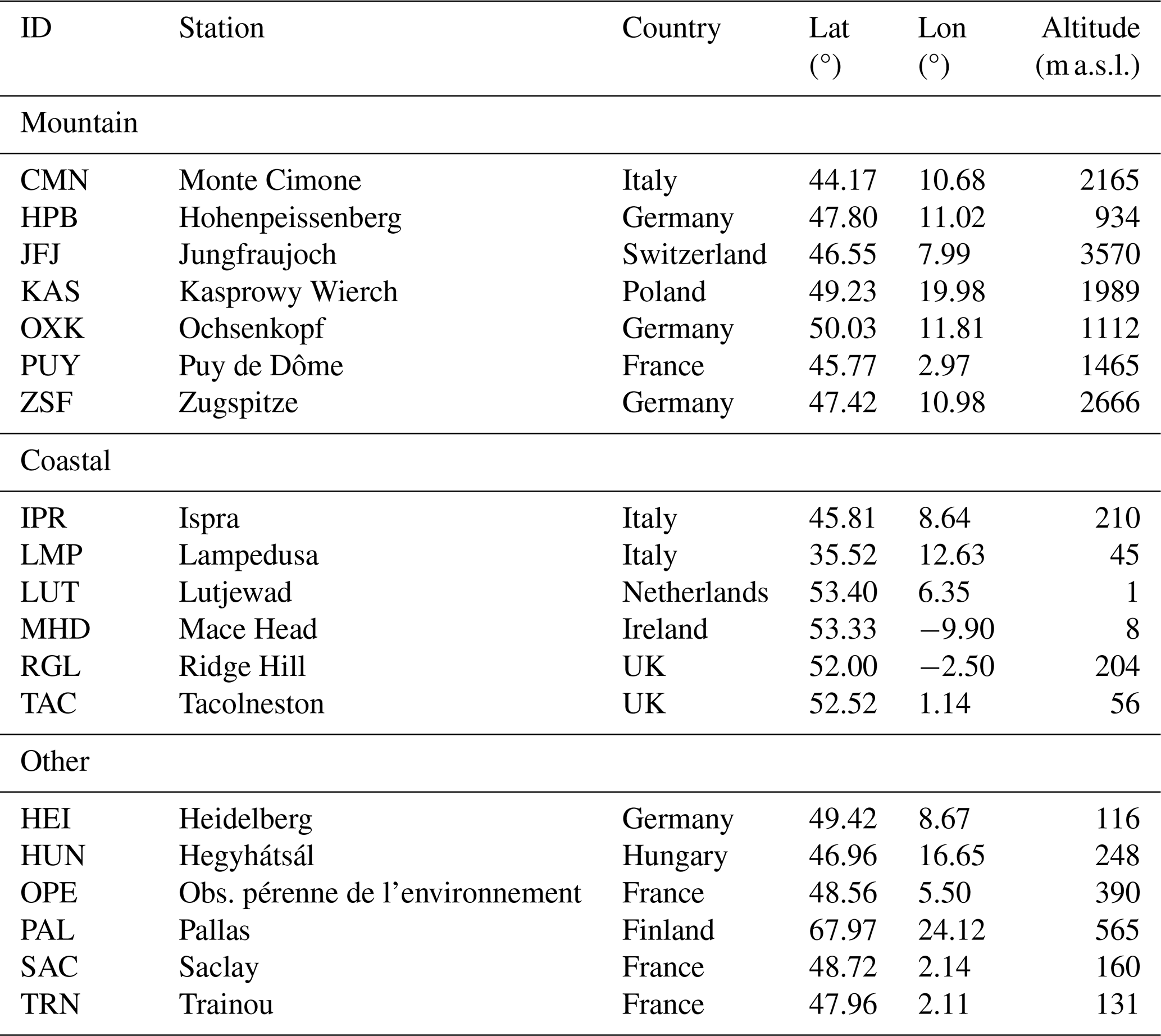
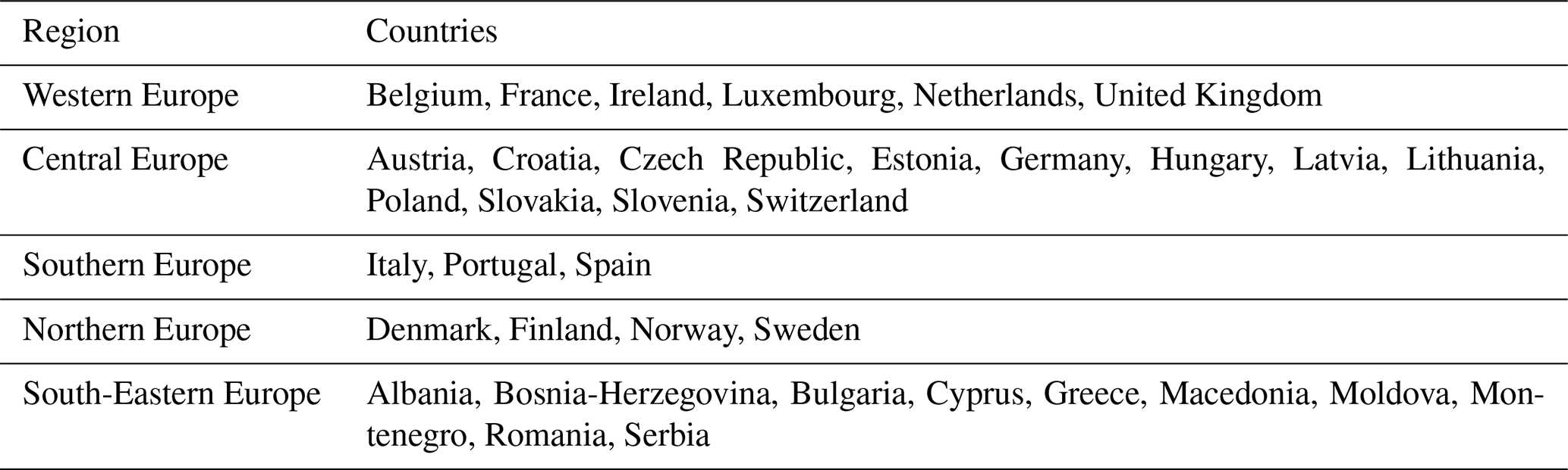
In addition to the comparison of the XCH₄ distributions of the TROPOMI products, we compare the TROPOMI-TCCON co-located observations for the seven TCCON stations listed in Table C1. The Total Carbon Column Observing Network (TCCON) is a network of ground-based stations equipped with similar high-resolution spectrometers (Bruker IFS) and using a common retrieval algorithm to ensure comparability of the measurements. The network consists of 28 operational sites, of which 7 are in the domain of this study. It is available at https://tccondata.org/ (last access: 22 July 2026). We use the last update of GGG2020 (Laughner et al., 2024). Previous studies have compared one or two TROPOMI products to TCCON observations (Hilbig et al., 2023; Balasus et al., 2023; Borsdorff et al., 2024; Lindqvist et al., 2024), but none of them have directly compared the 3 products all together.

To compare observed CH₄ total columns from TROPOMI and TCCON datasets, we consider the co-located observations that are within 1 h and 100 km of each other, with a maximum surface elevation difference of 250 m. For co-located observations, it is required to adjust the columns for the differences of vertical sensitivities and prior XCH₄ profiles used in the retrievals, using the TCCON profile as the common prior profile. Following Apituley et al. (2025), Schneising (2022) and Balasus et al. (2023), the vertical profiles of TCCON (51 levels) are interpolated on the TROPOMI layers l (20 layers for WFMD, 12 for SRON and BLENDED). The adjusted TROPOMI XCH₄ total column ${\widehat{y}}_{\mathrm{adj}}$ is thus, with y_a,TC and y_a,TR the TCCON and TROPOMI prior profiles, $\widehat{y}$ the TROPOMI XCH₄ total column and a the column averaging kernel:

$$\begin{array}{}\text{(C1)}& {\widehat{y}}_{\mathrm{adj}}=\widehat{y}+\sum _l{h}^l(\mathrm{1}-a^l)(y_{a,\mathrm{TC}}^l-y_{a,\mathrm{TR}}^l)\end{array}$$

The results of the comparison for 2019 are presented in Table C2 and Fig. C1. WFMD tends to overestimate methane concentrations, SRON has the lowest mean of the daily averaged difference but higher deviations and lower correlation in comparison to the other products. BLENDED observations align more closely with TCCON in terms of R² and RMSE, with a negative offset that is rather uniform across the stations. The average for individual stations are consistent with Balasus et al. (2023) and Hilbig et al. (2023) for SRON and BLENDED. However, they differ from the results of Borsdorff et al. (2024) and Lindqvist et al. (2024) for WFMD and from the results of Hilbig et al. (2023) for SRON. Overall, the values of the differences between TROPOMI and TCCON XCH₄ fall in the range [−25, +25] ppb. Moreover, the relative accuracy (standard deviation of the mean local offsets relative to TCCON at the individual sites) of TROPOMI products shown in Table C2 are below the 10 ppb threshold deemed suitable for regional inversions by Buchwitz et al. (2015). BLENDED and WFMD have lower relative accuracies (3.1 and 3.3 ppb) than SRON (4.8 ppb).

Analysis of individual stations reveals similar patterns for those located in Western Europe (Bremen, Karlsruhe, Orléans and Paris). For these stations, SRON and WFMD show comparable distributions (with WFMD values slightly higher), while BLENDED systematically produces lower median values, consistently with the comparison of XCH₄ distributions detailed in Sect. 3.1. A similar pattern can be seen in Nicosia, except for SRON higher values. All the products have a similar positive offset in Garmisch in comparison to other Western Europe stations. For this station, located in the Northern Alps, the offset is likely due to a bias associated with albedo or difference in the altitude of the ground pixel of the satellite and the station.

Figure S7 shows a seasonally-resolved version of Fig. C1, and Fig. S8 shows the time series of the TROPOMI-TCCON difference for key sites. Seasonal distributions and time series indicate a low seasonal dependency in the differences, apart from Sodankylä. In this high-latitude station in Finland, the bias in 2019 is positive during spring, and negative in autumn, consistent with the findings of Lindqvist et al. (2024). This seasonal variation is only present in 2019. Due to this temporal variations and to the limited number of co-located observations at this latitude, the deviations of the TROPOMI-TCCON differences are amplified, especially for SRON which has the largest seasonal variations. These results highlight the challenges of using TROPOMI at high latitudes, where coverage is sparse, and uncertainties are large.

Table C1 TCCON stations used for the evaluation.

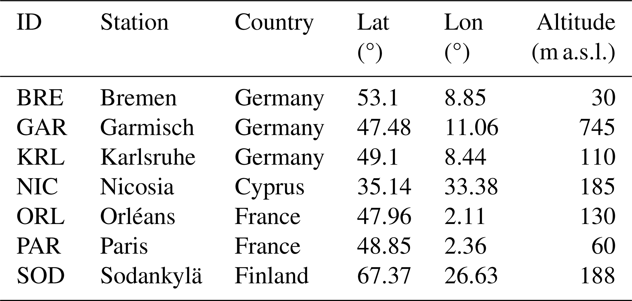
Table C2 Mean and RMSE of the daily averaged difference TROPOMI-TCCON, as well as the correlation (R²) and the relative accuracy of the TROPOMI products relative to TCCON, over the co-located observations at the TCCON stations in 2019. The relative accuracy is the standard deviation of the mean local offsets relative to TCCON at the individual sites.

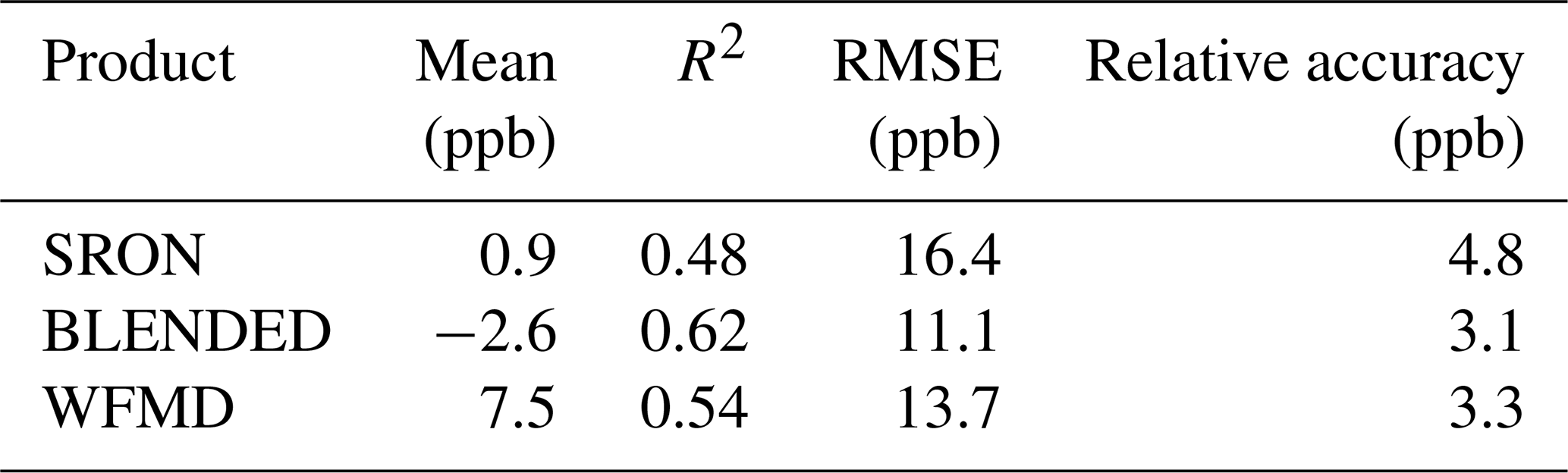
Figure C1 Median and quartiles of the daily averaged differences between TROPOMI and TCCON XCH₄ (ppb) for each station selected for the evaluation, in 2019.

Appendix D: Additional figures

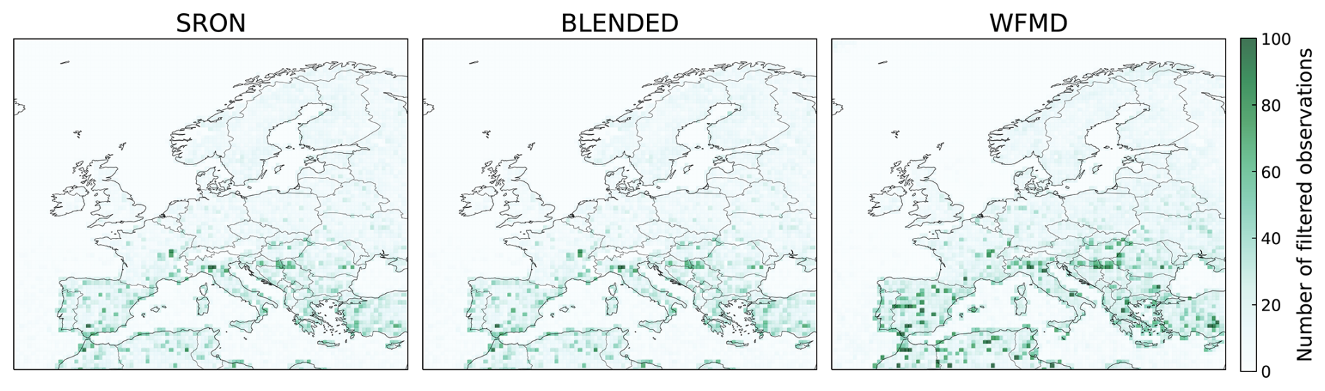
Figure D1 Count of observations that have been filtered in the post-processing of the TROPOMI products, as described in Sect. 2.4.2

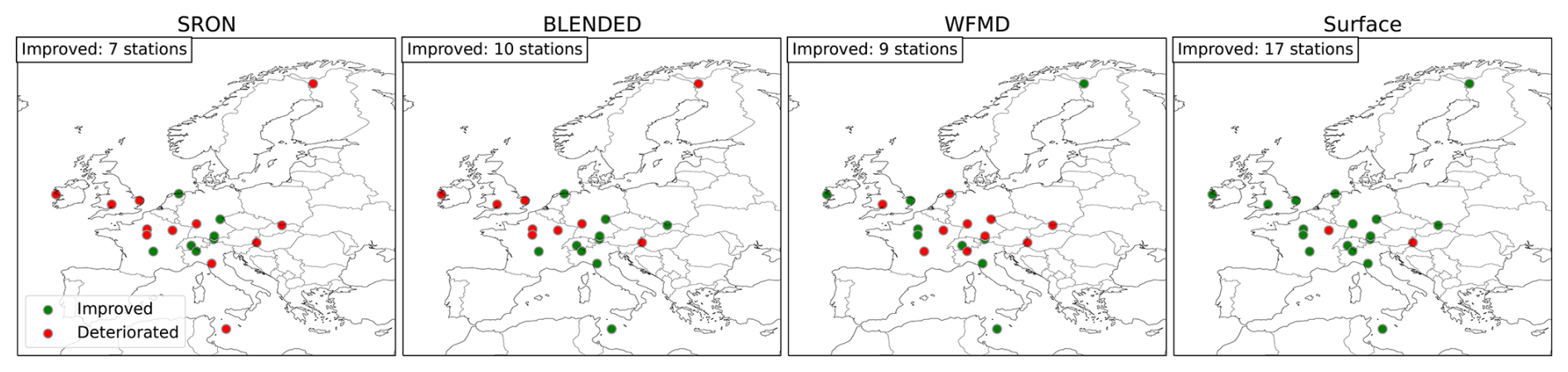
Figure D2 Evaluation map of the satellite-based and surface-based inversions: green (resp. red) circles are the surface stations for which the posterior simulated concentrations are in average closer (resp. further away) to the observations than the prior ones.

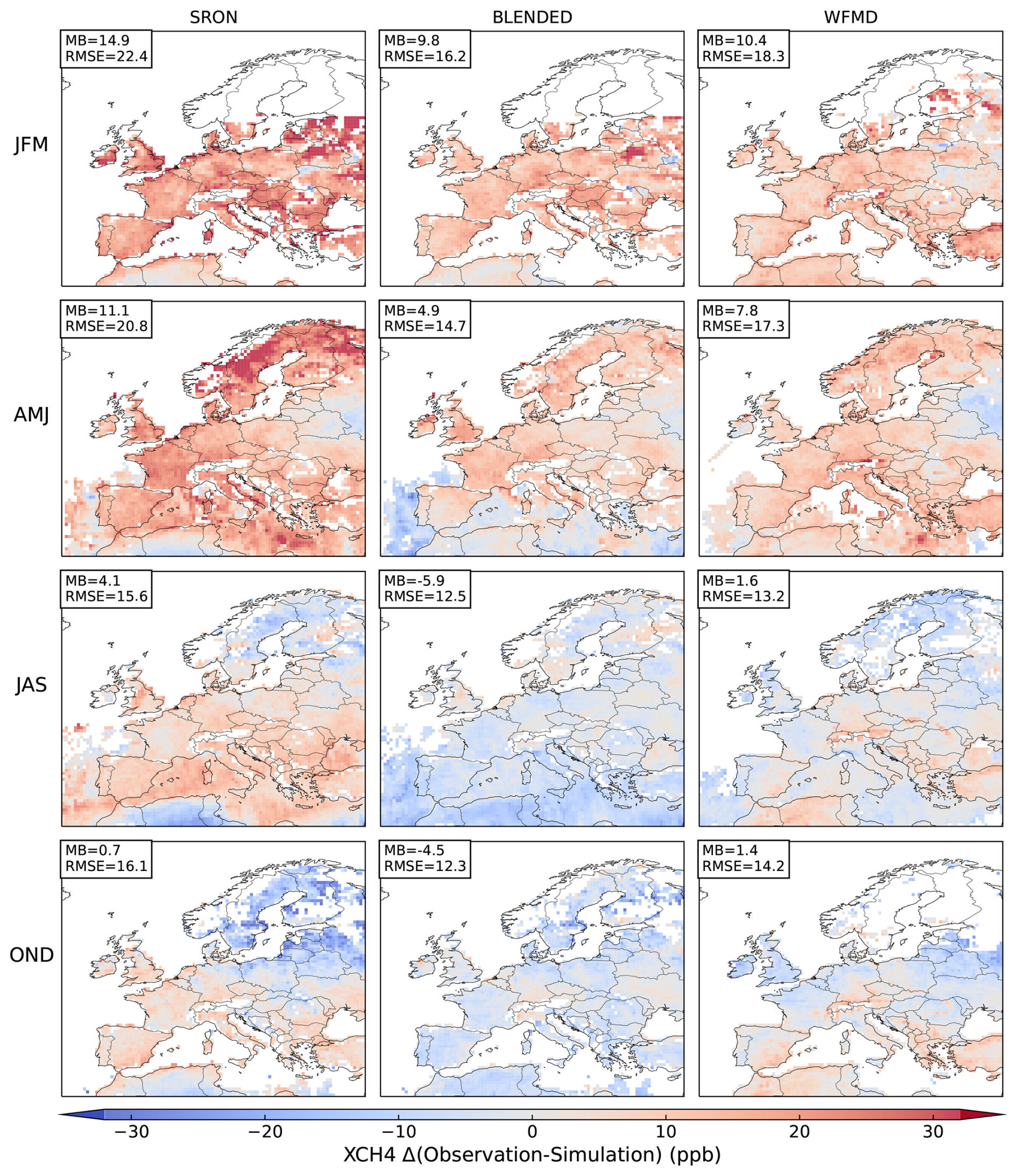
Figure D3 Seasonal average difference between TROPOMI observed concentration and CHIMERE simulated equivalent. MB is the mean bias and RMSE the root mean square error. Units are pbb. JFM, AMJ, JAS and OND are acronyms referring to the months of each season.

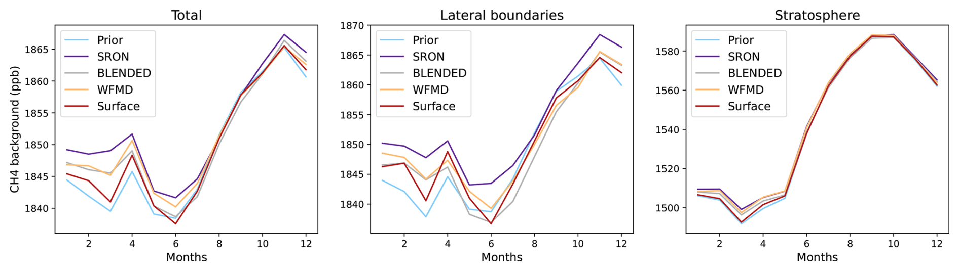
Figure D4 Time series of monthly averaged increments of the components of the background, for the 4 inversions presented in Sect. 2.4.2. The first panel shows the time series of averaged total columns, the second panel those with only the pixels used as lateral boundary conditions, and the third panel shows the time series of average stratosphere column (for pressures >200 hPa).

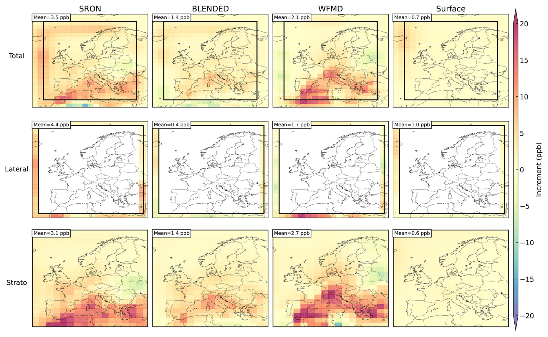
Figure D5 Increments of the components of the background, for the 4 inversions presented in Sect. 2.4.2. The components of the background are the same as in Fig. D4: averaged total columns (first row), pixels used as lateral boundary conditions (second row), and average stratosphere column for pressures >200 hPa (third row).