Ozone dry deposition through plant stomata: multi-model comparison with flux observations and the role of water stress as part of AQMEII4 Activity 2

A substantial portion of tropospheric O₃ dry deposition occurs after diffusion of O₃ through plant stomata. Simulating stomatal uptake of O₃ in 3D atmospheric chemistry models is important in the face of increasing drought-induced declines in stomatal conductance and enhanced ambient O₃. Here, we present a comparison of the stomatal component of O₃ dry deposition (eg_s) from chemical transport models and estimates of eg_s from observed CO₂, latent heat, and O₃ flux. The dry deposition schemes were configured as single-point models forced with data collected at flux towers. We conducted sensitivity analyses to study the impact of model parameters that control stomatal moisture stress on modeled eg_s. Examining six sites around the Northern Hemisphere, we find that the seasonality of observed flux-based eg_s agrees with the seasonality of simulated eg_s at times during the growing season, with disagreements occurring during the later part of the growing season at some sites. We find that modeled water stress effects are too strong in a temperate–boreal transition forest. Some single-point models overestimate summertime eg_s in a seasonally water-limited Mediterranean shrubland. At all sites examined, modeled eg_s was sensitive to parameters that control the vapor pressure deficit stress. At specific sites that experienced substantial declines in soil moisture, the simulation of eg_s was highly sensitive to parameters that control the soil moisture stress. The findings demonstrate the challenges in accurately representing the effects of moisture stress on the stomatal sink of O₃ during observed increases in dryness due to ecosystem-specific plant–resource interactions.

1 Introduction

Tropospheric ozone (O₃) is a secondary air pollutant formed through photochemical reactions involving biogenic and anthropogenic emissions of methane, non-methane volatile organic compounds (VOCs), carbon monoxide (CO), and nitrogen oxides (NO_x). Dry deposition of O₃ represents a substantial sink of tropospheric O₃ (Lelieveld and Dentener, 2000; Stevenson et al., 2006; Wild, 2007; Young et al., 2013), and the simulation of O₃ deposition velocity, V_d, can impact the simulation of O₃ concentrations near the surface, propagating the atmospheric vertical O₃ profile upward (Baublitz et al., 2020; Clifton et al., 2020b). Since dry deposition directly impacts ambient O₃ concentrations, modeling the multiple processes involved in dry deposition is an important component of 3D atmospheric chemistry models (Hardacre et al., 2015; Clifton et al., 2023). An important contribution to dry deposition occurs with the diffusion of O₃ through plant stomata, tiny pores on leaf surfaces which facilitate the exchange of gases such as CO₂, H₂O, and O₃. O₃ can degrade to reactive oxygen species in the leaf apoplast and react with compounds after stomatal uptake transports O₃ to the intercellular spaces of leaves (Baier et al., 2005; Dizengremel et al., 2009; Wedow et al., 2021). The stomatal sink of O₃ makes stomatal conductance, determined largely by the aperture of stomatal pores and stomatal density, a key component of modeling dry deposition of O₃.

The ability of plants to sense environmental changes can result in osmotic adjustments that lead to changes in guard cell turgor, stomatal aperture, and eventually stomatal conductance, and through this mechanism, stomatal conductance can respond to changing environmental conditions on timescales as short as minutes (Hetherington and Woodward, 2003; Lawson and Vialet-Chabrand, 2019). Stomatal conductance responds to changes in soil moisture, photosynthetically active radiation (PAR), the vapor pressure deficit (VPD) between the interior of the leaf and the atmosphere, and intercellular CO₂ concentrations (Lawson, 2009; Lawson and Vialet-Chabrand, 2019; Grossiord et al., 2020; Matthews et al., 2020). O₃ uptake itself has been shown to impact stomatal conductance, possibly through bursts of reactive oxygen species in guard cells and impacting biochemical pathways, including those involved in stomatal sensitivity to soil drying (Wilkinson and Davies, 2009, 2010; Vahisalu et al., 2010; Lombardozzi et al., 2012b). Many factors of global change such as rising ambient CO₂ concentrations, increasing temperatures, and the increasing severity and frequency of droughts (Dai, 2013; Zhao and Dai, 2022) are likely to impact stomatal conductance (Liang et al., 2023). Thus, in addition to the photosynthetic response, the stomatal response to global change could be an important pathway by which global change impacts major components of the carbon and the water cycle such as photosynthesis and transpiration (Hetherington and Woodward, 2003; Marchin et al., 2023). Therefore, simulating the stomatal response to the environment is a critical component of many land surface models, and a large variety of stomatal conductance models are implemented (Damour et al., 2010; Franks et al., 2018; Sabot et al., 2022). Since the dry deposition of O₃ through stomata is substantial, many of these stomatal conductance models are also used to simulate the stomatal component of O₃ dry deposition in the atmospheric chemistry models that we analyze in this study.

Stomatal uptake of O₃ makes up to 45 %–75 % of dry deposition during the growing season (Kurpius and Goldstein, 2003; Stella et al., 2011, 2013; Clifton et al., 2020a), with non-stomatal processes like uptake to soil and leaf cuticles and within-canopy chemistry contributing to the rest of the dry deposition. Furthermore, stomatal sensitivity to global change factors has been shown to impact tropospheric O₃ concentrations (Andersson and Engardt, 2010; Clifton et al., 2020b; Lin et al., 2020). For example, drought-induced declines in stomatal conductance can result in increases in O₃ pollution (Emberson et al., 2013; Anav et al., 2018; Clifton et al., 2020b; Lin et al., 2020). Proper representation of the stomatal component of O₃ V_d in 3D atmospheric chemistry models is likely important for predicting O₃ concentrations in light of what is often referred to as the “climate penalty” on air quality, part of which includes increasing O₃ concentrations during drought conditions regardless of local air quality regulations (Wang et al., 2017; Lin et al., 2020).

Comparisons and evaluations of dry deposition schemes and their components, such as the stomatal component, are essential to improve the monitoring and predictive abilities of 3D atmospheric chemistry models (Dennis et al., 2010; He et al., 2021). A study by Hardacre et al. (2015) comparing O₃ V_d and flux across global 3D atmospheric chemistry models stressed the importance of examination of the components of O₃ dry deposition. Wu et al. (2018) examined five dry deposition schemes at one site and suggested that the different representations of the stomatal and non-stomatal pathways contribute more to disagreements between model-simulated V_d values compared to the different representations of the turbulent transport of O₃ to the land surface. Previous comparisons of dry deposition schemes also reveal that the choice of driving variables related to moisture stress, such as near-surface VPD, leaf water potential, volumetric soil water content, or soil water potential, can be a source of disagreement between simulations of stomatal conductance (Büker et al., 2012; Visser et al., 2021; Huang et al., 2022; Sun et al., 2022; Wong et al., 2022; Clifton et al., 2023). Such evaluations often rely on observed O₃ flux and V_d at flux towers and/or observation-based inversions of the components of V_d (Fares et al., 2010; Hardacre et al., 2015; Clifton et al., 2017; Visser et al., 2021; Wong et al., 2022). Observations of latent heat flux and micrometeorological data collected over the footprint of flux towers instrumented with gas analyzers and sonic anemometers allow an inversion of the surface conductance to water vapor (Shuttleworth et al., 1984; Gerosa et al., 2007; Novick et al., 2016; Clifton et al., 2017; Medlyn et al., 2017; Knauer et al., 2018b; Vermeuel et al., 2021; Wehr and Saleska, 2021). While these estimates do not represent a direct measurement of stomatal conductance, they offer an estimate of ecosystem-scale surface conductance to water vapor, and the stomatal component is assumed to be dominant when transpiration dominates evapotranspiration. Such estimates of stomatal conductance have been used to understand the importance of driving variables such as VPD and soil moisture for the site-scale stomatal component of O₃ dry deposition (e.g., Visser et al., 2021), but not to systematically evaluate many dry deposition schemes across many sites worldwide with a focus on comparing how models specify the stomatal sensitivity to driving variables. This keeps us from a full understanding of the strengths and challenges of the simulation of stomatal conductance across a large variety of dry deposition schemes. Particularly, many model parameters, within the diversity of stomatal conductance models that are used in dry deposition schemes, control the effects of moisture stress drivers on stomatal conductance, and the sensitivity of stomatal dry deposition to these parameters across a range of ecosystems is unclear.

The Air Quality Model Evaluation International Initiative 4 (AQMEII4) was designed to compare and evaluate the representation of dry deposition, including the individual contributing processes, in atmospheric chemistry models (Galmarini et al., 2021; Clifton et al., 2023). Activity 2 (hereinafter A2) isolated 18 dry deposition schemes implemented in various atmospheric chemistry models as single-point models and forced the single-point models with micrometeorological and other environmental data from eight flux tower sites (Clifton et al., 2023). Clifton et al. (2023) used observed O₃ V_d at the sites to evaluate modeled O₃ V_d and carried out a detailed comparison of the components of deposition velocity. They find that simulated O₃ V_d can be similar among models, while the relative contribution of each component can be quite different among models (Clifton et al., 2023). Conversely, simulated V_d can be quite variable among models when the relative contribution of the components is similar among models (Clifton et al., 2023). However, the stomatal component of O₃ deposition velocity simulated by the single-point models was not compared with observed CO₂ and latent-heat-flux-based estimates of stomatal conductance, which may offer observation-based insights into some of the among-model discrepancies noted by Clifton et al. (2023).

Here, we carry out a model comparison of the stomatal component of O₃ V_d with observed flux-based estimates as part of AQMEII4 A2. We carry out the comparison across six Northern Hemisphere sites consisting of boreal, temperate, and temperate–boreal transition forests along with an eastern Mediterranean shrubland and a temperate grassland. Particularly, we focus on parameter and process sensitivity in both model evaluation and comparison. We isolate two case studies of observed substantial decreases in soil moisture and increases in near-surface VPD to understand the simulation of the stomatal component during times of increased soil and air dryness. Finally, we conducted sensitivity analyses perturbing the values of parameters that control stomatal moisture stress to isolate the impact of parameter choice. We address the following research questions.

1. How does the stomatal component of O₃ V_d simulated by single-point models compare with the estimates from observed latent heat and CO₂ flux?

2. How does the specification of moisture stress in single-point models impact the agreement in the stomatal component of O₃ V_d between single-point model simulations and flux-based estimates during times of increased atmospheric or soil dryness?

3. In dry deposition schemes, how do stomatal moisture stress parameters affect the agreement between single-point models and observed flux-based estimates?

2 Methods

2.1 Two major classes of stomatal conductance models used in O₃ dry deposition schemes

Clifton et al. (2023) listed the detailed equations of all stomatal conductance models used in the single-point models evaluated in AQMEII4 A2. There are two major classes of stomatal conductance models implemented. The first class is based on the model proposed by Jarvis et al. (1976) (hereinafter Jarvis-type). Jarvis-type models use separate stress functions for different environmental conditions and specify the severity of a particular environmental stress with values which range from no stress to maximum stress. In some Jarvis-type models, individual stress functions are multiplied and serve to attenuate the maximum stomatal conductance that can be expected under ideal growing conditions. In other Jarvis-type models, the maximum value from a set of stress functions is chosen to attenuate the maximum stomatal conductance. A range of environmental stresses are implemented among the AQMEII4 A2 dry deposition schemes that use Jarvis-type stomatal conductance models. Some schemes implement a few stress functions with incoming solar radiation and air temperature based on the classic Wesely (1989) dry deposition scheme, while others implement many more (Xiu and Pleim, 2001; Zhang et al., 2003). The general form of the Jarvis-type models for stomatal resistance to water vapor ($R_{\mathrm{s},{\mathrm{H}}_{\mathrm{2}}\mathrm{O}}$; s m⁻¹) (a conductance is the inverse of a resistance) is

$$\begin{array}{}\text{(1)}& {\displaystyle }{\displaystyle }{R}_{\mathrm{s},{\mathrm{H}}_{\mathrm{2}}\mathrm{O}}={\displaystyle \frac{R_{\mathrm{s},{\mathrm{H}}_{\mathrm{2}}\mathrm{O},\text{ideal}}}{f\left(x_{\mathrm{1}}\right)f\left(x_{\mathrm{2}}\right)f\left(x_{\mathrm{3}}\right)f\left(x_{\mathrm{4}}\right)}},\end{array}$$

where $R_{\mathrm{s},{\mathrm{H}}_{\mathrm{2}}\mathrm{O},\text{ideal}}$ is the stomatal resistance to H₂O under ideal environmental conditions (s m⁻¹), and f(x) denotes a function which controls the strength of the stress that is imposed by an environmental variable, x. Environmental variables related to air moisture include the difference between air vapor pressure and saturation vapor pressure at air temperature at measurement height (VPD_air; kPa), leaf-level relative humidity (RH_l), and relative humidity at measurement height (${\text{RH}}_{z_{\mathrm{m}}}$). Environmental variables related to soil moisture or plant water status include volumetric soil water content (w₂; m³ m⁻³), soil matric potential (ψ_soil; kPa), and leaf water potential (ψ_leaf; MPa). A number of equations and parameters can be used to calculate the value of f(x). An example of a Jarvis-type model, implemented in the CMAQ M3Dry model (Xiu and Pleim, 2001), is

$$\begin{array}{}\text{(2)}& {\displaystyle }{\displaystyle }{R}_{\mathrm{s},{\mathrm{H}}_{\mathrm{2}}\mathrm{O}}={\displaystyle \frac{R_{\mathrm{s},{\mathrm{H}}_{\mathrm{2}}\mathrm{O},\text{ideal}}}{\text{LAI}f\left(\text{PAR}\right)f\left(w_{\mathrm{2}}\right)f\left({\text{RH}}_{\mathrm{l}}\right)f\left(T_{\text{air}}\right)}},\end{array}$$

where PAR is photosynthetically active radiation ($\mathrm{\mu }\mathrm{mol}{\mathrm{m}}^{-\mathrm{2}}{\mathrm{s}}^{-\mathrm{1}}$), T_air is air temperature (°C), and LAI is leaf area index (m² m⁻²).

The second class of stomatal conductance models used in the AQMEII4 A2 dry deposition schemes couple net photosynthesis with stomatal conductance using the models of Ball et al. (1987), Leuning (1995), or Medlyn et al. (2011). Net photosynthesis is simulated with the widely used Farquhar et al. (1980) biochemical photosynthesis model or models similar to it. An example of a net photosynthesis coupled stomatal conductance model used in some of the TEMIR single-point models is (Ball et al., 1987; Tai et al., 2024)

$$\begin{array}{}\text{(3)}& {\displaystyle }{\displaystyle }{R}_{\mathrm{s},{\mathrm{CO}}_{\mathrm{2}}}={\left({\mathit{\beta }}_t{g}_o+g_{\mathrm{1}}{\displaystyle \frac{A_{\mathrm{n}}{\text{RH}}_{z_{\mathrm{m}}}}{\frac{P_{{\mathrm{CO}}_{\mathrm{2}},\mathrm{l}}}{P_{\mathrm{a}}}}}\right)}^{-\mathrm{1}}{\displaystyle \frac{P_{\mathrm{a}}}{R{\mathit{\theta }}_{\mathrm{a}}}},\end{array}$$

where $R_{\mathrm{s},{\mathrm{CO}}_{\mathrm{2}}}$ is the stomatal resistance to CO₂ (s m⁻¹), g_o is the minimum conductance ($\mathrm{mol}{\mathrm{m}}^{-\mathrm{2}}{\mathrm{s}}^{-\mathrm{1}}$), g₁ is a slope parameter commonly used in the models of Leuning (1995), Ball et al. (1987), and Medlyn et al. (2011) (the interpretation of g₁ is different among models), A_n is net photosynthesis ($\mathrm{mol}{\mathrm{m}}^{-\mathrm{2}}{\mathrm{s}}^{-\mathrm{1}}$), $P_{{\mathrm{CO}}_{\mathrm{2}},\mathrm{l}}$ is CO₂ partial pressure at the leaf surface (Pa), P_a is the air pressure (Pa), R is the universal gas constant ($\mathrm{J}{\mathrm{mol}}^{-\mathrm{1}}{\mathrm{K}}^{-\mathrm{1}}$), and θ_a is potential temperature (K). The soil moisture stress factor, β_t, is calculated as

$$\begin{array}{}\text{(4)}& {\displaystyle }{\displaystyle }{\mathit{\beta }}_t=\left\{\begin{array}{ll}\mathrm{1},& {\mathit{\psi }}_{\text{soil}}>{\mathit{\psi }}_{\text{soil,fc}}\\ \frac{{\mathit{\psi }}_{\text{soil,wlt}}-{\mathit{\psi }}_{\text{soil}}}{{\mathit{\psi }}_{\text{soil,wlt}}-{\mathit{\psi }}_{\text{soil,fc}}},& {\mathit{\psi }}_{\text{soil,wlt}}\le {\mathit{\psi }}_{\text{soil}}\le {\mathit{\psi }}_{\text{soil,fc}}\\ \mathrm{0},& {\mathit{\psi }}_{\text{soil}}<{\mathit{\psi }}_{\text{soil,fc}},\end{array}\right.\end{array}$$

where ψ_soil,fc is the soil matric potential at field capacity (kPa), and ψ_soil,wlt is the soil matric potential at wilting point (kPa). Like the Jarvis-type models, participating net photosynthesis models vary in whether they employ ${\text{RH}}_{z_{\mathrm{m}}}$, RH_l, or VPD_air to incorporate the effects of air moisture on stomatal conductance. Soil moisture impacts are simulated with the use of ψ_soil or w₂ to calculate stress factors (e.g., β_t) among the net photosynthesis coupled models. In models that use ψ_soil in their soil moisture stress function, ψ_soil is estimated as a function of w₂ as

$$\begin{array}{}\text{(5)}& {\displaystyle }{\displaystyle }{\mathit{\psi }}_{\text{soil}}={\mathit{\psi }}_{\text{soil,sat}}{w}_{\mathrm{2}}^{-B},\end{array}$$

where ψ_soil,sat is the soil matric potential at saturation (kPa), and B is a site-specific parameter to convert w₂ to ψ_soil. $R_{\mathrm{s},{\mathrm{H}}_{\mathrm{2}}\mathrm{O}}$ is scaled to the stomatal resistance to O₃ using the ratio of O₃ diffusivity in air (m² s⁻¹) to H₂O diffusivity in air (m² s⁻¹). $R_{\mathrm{s},{\mathrm{CO}}_{\mathrm{2}}}$ is scaled to the stomatal resistance to O₃ using the ratio of O₃ diffusivity in air (m² s⁻¹) to CO₂ diffusivity in air (m² s⁻¹).

Both the net photosynthesis coupled models and the Jarvis-type models have a number of parameters that control the effect of soil and/or air moisture on stomatal conductance. Full descriptions of the single-point models in this study can be found in Clifton et al. (2023). We divide the two major classes of stomatal conductance models into four classes as net photosynthesis coupled models that include both soil and air moisture impacts through the use of ψ_soil, w₂, VPD_air, ${\text{RH}}_{z_{\mathrm{m}}}$, or RH_l (NP:SM/VPD/RH); Jarvis-type models that include both soil and air moisture impacts through the use of w₂, VPD_air, ${\text{RH}}_{z_{\mathrm{m}}}$, or RH_l (J:SM/VPD/RH); Jarvis-type models that only include VPD_air (J:VPD); and Jarvis-type models that do not include soil moisture or air moisture impacts (J:NoSM/VPD/RH). J:VPD models include the impact of plant water status through the use of ψ_leaf. However, ψ_leaf is only modeled as a function of solar radiation, and it is not coupled with ψ_soil. Therefore, we did not include it in the J:SM/VPD/RH class.

2.2 Stomatal conductance to O₃ estimated from observations of latent heat flux and net ecosystem exchange of CO₂

We calculated two separate estimates of stomatal conductance to O₃ ($G_{\mathrm{s},{\mathrm{O}}_{\mathrm{3}}}$) using observations of latent heat flux (λE) and net ecosystem exchange of CO₂ (NEE) at the flux towers. These flux observations are not used as forcing data for the single-point models. The first estimate is an inversion of the evaporation–resistance form of the Penman–Monteith (PM) equation (Monteith, 1981) as presented by Gerosa et al. (2005, 2007) to calculate the surface resistance to water vapor, $R_{\mathrm{s},{\mathrm{H}}_{\mathrm{2}}\mathrm{O},\text{PM}}$ (s m⁻¹), as

$$\begin{array}{}\text{(6)}& {\displaystyle }{\displaystyle }{R}_{\mathrm{s},{\mathrm{H}}_{\mathrm{2}}\mathrm{O},\text{PM}}={\displaystyle \frac{\mathit{\rho }{c}_{\mathrm{p}}\left[{\text{VPD}}_{\text{canopy-air}}\right]}{\mathit{\gamma }\mathit{\lambda }E}}-(R_{\mathrm{a}}+R_{\mathrm{b},{\mathrm{H}}_{\mathrm{2}}\mathrm{O}}),\end{array}$$

where λE is the latent heat flux (W m⁻²), ρ is the air density (kg m⁻³), c_p is the specific heat capacity of dry air at constant pressure ($\mathrm{J}{\mathrm{K}}^{-\mathrm{1}}{\mathrm{kg}}^{-\mathrm{1}}$), VPD_canopy-air is the vapor pressure difference between the evaporating canopy surface and the measurement height (kPa), γ is the psychrometric constant (kPa K⁻¹), R_a is the aerodynamic resistance to turbulent transfer (s m⁻¹), and $R_{\mathrm{b},{\mathrm{H}}_{\mathrm{2}}\mathrm{O}}$ is the quasi-laminar layer resistance to water vapor (s m⁻¹). VPD_canopy-air is calculated as

$$\begin{array}{}\text{(7)}& {\displaystyle }{\displaystyle }{\text{VPD}}_{\text{canopy-air}}=e_{\mathrm{s}}\left(T_{\mathrm{s}}\right)-e\left(z_{\mathrm{m}}\right),\end{array}$$

where e_s(T_s) is the saturation vapor pressure (kPa) at the temperature of the evaporating canopy surface (T_s; °C), and e(z_m) is the vapor pressure at the measurement height (kPa). e_s(T_s) is calculated using the Tetens formula:

$$\begin{array}{}\text{(8)}& {\displaystyle }{\displaystyle }{e}_{\mathrm{s}}\left(T_{\mathrm{s}}\right)=a\exp \left({\displaystyle \frac{b{T}_{\mathrm{s}}}{T_{\mathrm{s}}+c}}\right),\end{array}$$

where a=0.611 kPa, b=17.502, and c=240.97 °C. T_s was calculated as

$$\begin{array}{}\text{(9)}& {\displaystyle }{\displaystyle }{T}_{\mathrm{s}}=T_{\text{air}}+{\displaystyle \frac{H}{\mathit{\rho }{c}_{\mathrm{p}}}}(R_{\mathrm{a}}+R_{\mathrm{b},H}),\end{array}$$

where H is the sensible heat flux (W m⁻²), and R_b,H is the quasi-laminar layer resistance to heat (s m⁻¹).

The second stomatal conductance estimate fits a stomatal conductance model to the estimates of stomatal conductance from the PM inversion ($G_{\mathrm{s},{\mathrm{H}}_{\mathrm{2}}\mathrm{O},\text{PM}}=R_{\mathrm{s},{\mathrm{H}}_{\mathrm{2}}\mathrm{O},\text{PM}}^{-\mathrm{1}}$). We fit the Medlyn et al. (2011) leaf-level stomatal conductance model using gross primary productivity (GPP) as presented by Medlyn et al. (2017) and Knauer et al. (2018b):

$$\begin{array}{}\text{(10)}& {\displaystyle }{\displaystyle }{G}_{\mathrm{s},{\mathrm{H}}_{\mathrm{2}}\mathrm{O},\text{MED}}=G_o+\mathrm{1.6}\left(\mathrm{1}+{\displaystyle \frac{G_{\mathrm{1}}}{\sqrt{{\text{VPD}}_{\text{canopy-air}}}}}\right){\displaystyle \frac{\text{GPP}}{C_{\mathrm{a}}}},\end{array}$$

where $G_{\mathrm{s},{\mathrm{H}}_{\mathrm{2}}\mathrm{O},\text{MED}}$ is the stomatal conductance to H₂O ($\mathrm{mol}{\mathrm{m}}^{-\mathrm{2}}{\mathrm{s}}^{-\mathrm{1}}$), G_o is the minimum stomatal conductance to H₂O ($\mathrm{mol}{\mathrm{m}}^{-\mathrm{2}}{\mathrm{s}}^{-\mathrm{1}}$), G₁ is a parameter that is inversely related to intrinsic water use efficiency (kPa^0.5) (Medlyn et al., 2017), GPP is gross primary productivity ($\mathrm{\mu }\mathrm{mol}{\mathrm{m}}^{-\mathrm{2}}{\mathrm{s}}^{-\mathrm{1}}$), and C_a is the ambient CO₂ concentration (ppm). GPP was calculated by partitioning the NEE flux into GPP and ecosystem respiration, R_eco. Nighttime NEE is assumed to be entirely R_eco. NEE was partitioned using the R package REddyProc with a partitioning approach that uses the nighttime NEE flux to estimate a temporally varying R_eco–T_air relationship as (Reichstein et al., 2012; Wutzler et al., 2018; Stoy et al., 2006)

$$\begin{array}{ll}{\displaystyle }& {\displaystyle }{R}_{\text{eco}}\left(T_{\text{air}}\right)=R_{\text{Ref}}\\ \text{(11)}& {\displaystyle }& {\displaystyle }\times \exp \left[E_{\mathrm{0}}\left({\displaystyle \frac{\mathrm{1}}{T_{\text{air,Ref}}-T_{\text{air,0}}}}-{\displaystyle \frac{\mathrm{1}}{T_{\text{air}}-T_{\text{air,0}}}}\right)\right],\end{array}$$

where E₀ is the temperature sensitivity, T_air,0 is held constant at −46.02 °C, and T_air,Ref is held at 15 °C. The R_eco–T_air relationship is applied to daytime data to obtain estimates of R_eco during the day. Finally, R_eco estimates are used to estimate GPP as

$$\begin{array}{}\text{(12)}& {\displaystyle }{\displaystyle }\text{GPP}=R_{\text{eco}}-\text{NEE}.\end{array}$$

In order to estimate the G_o and G₁ parameters by fitting Eq. (10) to $G_{\mathrm{s},{\mathrm{H}}_{\mathrm{2}}\mathrm{O},\text{PM}}$, we limited the full data that was used for the AQMEII4 A2 to conditions when transpiration would dominate λE and the stomatal component would dominate the surface conductance to water vapor. To do this, we limited the data to daytime conditions when relative humidity is less than 80 %. Data collected during a precipitation event and 48 h after a precipitation event were removed. We also limited the data to conditions when sensible heat flux was positive to avoid stable atmospheric conditions. Finally, we removed unusually high values for $G_{\mathrm{s},{\mathrm{H}}_{\mathrm{2}}\mathrm{O},\text{PM}}$ determined by looking at growing-season daily box plots of $G_{\mathrm{s},{\mathrm{H}}_{\mathrm{2}}\mathrm{O},\text{PM}}$ at each site. The site-specific upper thresholds for $G_{\mathrm{s},{\mathrm{H}}_{\mathrm{2}}\mathrm{O},\text{PM}}$ are listed in Table 1. Table 1 also shows other flux tower site details. The Python-based open-source software SciPy was used to estimate G_o and G₁ through least-squares optimization using a Huber loss function to reduce the influence of outliers (Virtanen et al., 2020). Calculating $G_{\mathrm{s},{\mathrm{H}}_{\mathrm{2}}\mathrm{O},\text{MED}}$ and $G_{\mathrm{s},{\mathrm{H}}_{\mathrm{2}}\mathrm{O},\text{PM}}$ allowed us to use the GPP flux, which is partitioned from NEE calculated from the observed CO₂ flux. This adds an estimate of stomatal conductance driven by GPP in addition to a separate estimate driven by λE. Both the CO₂ flux and λE share the stomatal pathway in their total flux. In order to calculate $G_{\mathrm{s},{\mathrm{O}}_{\mathrm{3}},\text{PM}}$ and $G_{\mathrm{s},{\mathrm{O}}_{\mathrm{3}},\text{MED}}$, $G_{\mathrm{s},{\mathrm{H}}_{\mathrm{2}}\mathrm{O},\text{PM}}$ and $G_{\mathrm{s},{\mathrm{H}}_{\mathrm{2}}\mathrm{O},\text{MED}}$ were scaled by the ratio of O₃ diffusivity ($D_{{\mathrm{O}}_{\mathrm{3}}}$) and H₂O diffusivity ($D_{{\mathrm{H}}_{\mathrm{2}}\mathrm{O}}$). The ratio $\frac{D_{{\mathrm{O}}_{\mathrm{3}}}}{D_{{\mathrm{H}}_{\mathrm{2}}\mathrm{O}}}$ was set as 0.61. All of the analysis in this paper uses daytime flux tower data and single-point model simulations.

Table 1 Description of the observational data used at each flux tower.

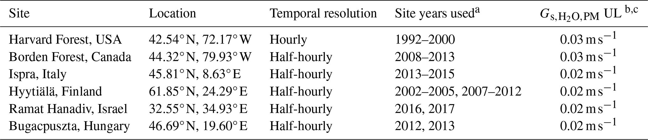
^a Figure S1 displays the months with available observations during each year used. ^b $G_{\mathrm{s},{\mathrm{H}}_{\mathrm{2}}\mathrm{O},\text{PM}}$ is the stomatal conductance to H₂O using the Penman–Monteith inversion. ^c $G_{\mathrm{s},{\mathrm{H}}_{\mathrm{2}}\mathrm{O},\text{PM}}$ UL stands for the upper limit applied to $G_{\mathrm{s},{\mathrm{H}}_{\mathrm{2}}\mathrm{O},\text{PM}}$. A description of the selection of the upper limit is provided in Sect. 2.2.

2.2.1 Effective stomatal conductance to O₃

The (half-)hourly deposition velocity of O₃, V_d, can be calculated from measurements of O₃ flux and concentrations at the flux tower sites as

$$\begin{array}{}\text{(13)}& {\displaystyle }{\displaystyle }{V}_{\mathrm{d}}={\displaystyle \frac{F_{{\mathrm{O}}_{\mathrm{3}}}}{[{\mathrm{O}}_{\mathrm{3}}{]}_{z_{\mathrm{m}}}}},\end{array}$$

where $F_{{\mathrm{O}}_{\mathrm{3}}}$ is the flux of O₃ measured at a flux tower site, and $[{\mathrm{O}}_{\mathrm{3}}{]}_{z_{\mathrm{m}}}$ is the O₃ concentration measured at the height of the instrument. The effective stomatal conductance to O₃ (eg_s) quantifies the amount of O₃ V_d that can be attributed to the stomatal component, and it is used to compare the contribution of a given depositional pathway (e.g., stomatal uptake) across models with differences in resistance schemes (Paulot et al., 2018; Clifton et al., 2020b; Galmarini et al., 2021). The single-point model simulations of eg_s are archived with AQMEII4 A2. It is important to note that the exact calculation of the effective conductance for a given pathway from the single-point models depends on the resistance framework used (Galmarini et al., 2021).

To compare eg_s from the single-point models and the observed flux-based estimates, we calculated eg_s from the (half-)hourly observed flux-based estimates, $G_{\mathrm{s},{\mathrm{O}}_{\mathrm{3}},\text{PM}}$ and $G_{\mathrm{s},{\mathrm{O}}_{\mathrm{3}},\text{MED}}$, as

$$\begin{array}{}\text{(14)}& {\displaystyle }& {\displaystyle }{\text{eg}}_{\mathrm{s},\text{PM}}={\displaystyle \frac{G_{\mathrm{s},{\mathrm{O}}_{\mathrm{3}},\text{PM}}}{G_{\mathrm{c}}}}{V}_{\mathrm{d}},\text{(15)}& {\displaystyle }& {\displaystyle }{\text{eg}}_{\mathrm{s},\text{MED}}={\displaystyle \frac{G_{\mathrm{s},{\mathrm{O}}_{\mathrm{3}},\text{MED}}}{G_{\mathrm{c}}}}{V}_{\mathrm{d}},\end{array}$$

where G_c is the canopy conductance to O₃ ($\mathrm{1}/R_{\mathrm{c},{\mathrm{O}}_{\mathrm{3}}}$). $R_{\mathrm{c},{\mathrm{O}}_{\mathrm{3}}}$ is calculated as the residual in $V_{\mathrm{d}}^{-\mathrm{1}}$ after calculating R_a and the quasi-laminar boundary layer resistance to O₃ ($R_{\mathrm{b},{\mathrm{O}}_{\mathrm{3}}}$; s m⁻¹) using the following big-leaf resistance framework:

$$\begin{array}{}\text{(16)}& {\displaystyle }{\displaystyle }{R}_{\mathrm{c},{\mathrm{O}}_{\mathrm{3}}}=V_{\mathrm{d}}^{-\mathrm{1}}-R_{\mathrm{a}}-R_{\mathrm{b},{\mathrm{O}}_{\mathrm{3}}}.\end{array}$$

R_a was calculated as (Verma, 1989; Knauer et al., 2018a)

$$\begin{array}{}\text{(17)}& {\displaystyle }{\displaystyle }{R}_{\mathrm{a}}={\displaystyle \frac{u\left(z_{\mathrm{m}}\right)}{u{*}^{\mathrm{2}}}},\end{array}$$

where u(z_m) is the wind speed (m s⁻¹) at the measurement height and u* is the friction velocity (m s⁻¹). $R_{\mathrm{b},{\mathrm{O}}_{\mathrm{3}}}$ is calculated as

$$\begin{array}{}\text{(18)}& {\displaystyle }{\displaystyle }{R}_{\mathrm{b},{\mathrm{O}}_{\mathrm{3}}}={\displaystyle \frac{\mathrm{2}}{ku*}}{\left({\displaystyle \frac{\mathit{\text{Sc}}}{\mathit{\text{Pr}}}}\right)}^{\mathrm{2}/\mathrm{3}},\end{array}$$

where k is the von Kármán constant (0.4), Sc is the Schmidt number (the ratio of kinematic viscosity of air to the molecular diffusivity of O₃), and Pr is the Prandtl number (the ratio of kinematic viscosity to thermal diffusivity).

To answer question 1, we calculated monthly mean eg_s from each single-point model and compared the averages to the monthly mean eg_s,PM and eg_s,MED inferred from observations as was done for total O₃ V_d in Clifton et al. (2023). We calculated monthly averages using all available years at a site. Therefore, when multiple years of data are available for a month, the monthly mean is a multiyear monthly mean. Ramat Hanadiv and Bugacpuszta only have 1 year of data for certain months of the year (Fig. S1 in the Supplement). We also compared the minimum, maximum, and central range of single-point modeled eg_s monthly averages with monthly mean eg_s,PM and eg_s,MED as Clifton et al. (2023) introduced for evaluating total O₃ V_d from these single-point models. We calculated the interquartile range (IQR) of the monthly averages from all single-point models, and we call the IQR the “central range” throughout the paper.

2.3 Isolating times of water stress for case studies

We chose two case studies to address question 2 by comparing the agreement between single-point modeled eg_s and observed flux-based eg_s during times of water stress: Borden Forest and Ramat Hanadiv. These case studies were chosen because they represent times when there was substantial disagreement in eg_s among models and between models and observed flux-based estimates, eg_s,PM and eg_s,MED, and the specification of moisture stress appeared to be a source of the variability. The first case study is at Borden Forest, Canada. The monthly mean soil volumetric water content measured at 50 cm depth fell below the model-specified wilting point during July 2011 and 2012 and September 2009, 2010, and 2011 at Borden Forest. July 2011 and 2012 also exhibit high mean VPD_air along with low mean soil volumetric water content (Fig. S1). Therefore, we used July 2011 and 2012 at Borden Forest as the first case study and compared simulated eg_s with eg_s,PM and eg_s,MED to understand if the flux-based eg_s supports the single-point modeled eg_s during this time. The second case study is at Ramat Hanadiv, Israel, a seasonally dry shrubland which experiences sharp declines in soil moisture and increases in VPD_air during the dry summer months (Fig. S1). Clifton et al. (2023) showed large divergence between single-point modeled and observed V_d at Ramat Hanadiv during the dry summer months. The seasonally dry months provided a case where we were able to study if models capture eg_s during conditions when the vegetation experiences substantial water stress at this shrubland.

2.4 Sensitivity of single-point simulated eg_s to parameters that control stomatal moisture stress

Sensitivity simulations were conducted to isolate the impact of moisture stress parameters on single-point modeled eg_s. The parameters related to moisture stress from many participating dry deposition schemes were perturbed along a range of values listed in Table 2. Some parameters control the strength of the soil moisture stress and the strength of the VPD_air stress. Other parameters control other plant ecophysiological properties such as the relationship between net photosynthesis and stomatal conductance or the intrinsic water-use efficiency. Additionally, we perturbed the $R_{\mathrm{s},{\mathrm{H}}_{\mathrm{2}}\mathrm{O},\text{ideal}}$ and $G_{\mathrm{s},{\mathrm{H}}_{\mathrm{2}}\mathrm{O},\text{max}}$ parameters as J:NoSM/VPD/RH models do not include moisture stress variables. Lastly, VPD_air and RH_l stress functions in some J:SM/VPD/RH models did not have parameters. For these models, we perturbed the value of the stress functions, f(VPD) and f(RH_l), to test the impact of varying the strength of the VPD_air and RH_l stress.

Table 2 A list of parameters related to moisture stress used in the dry deposition schemes. The “Values” column lists the range of the values used in the sensitivity analysis during which the values of a given parameter were changed to values within the range listed.

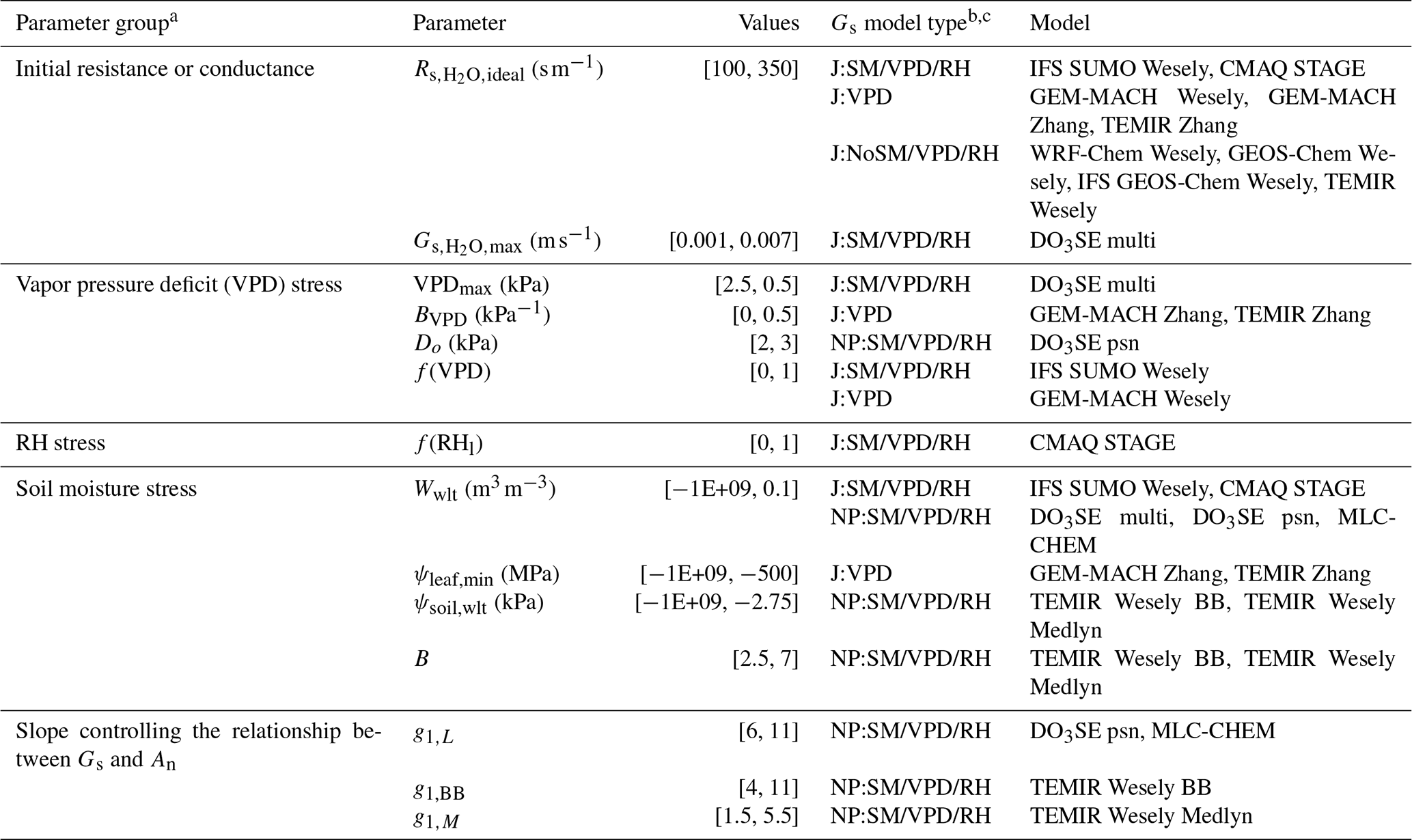
^a G_s is stomatal conductance. A_n is net photosynthesis. VPD is VPD_air. RH can be ${\text{RH}}_{z_{\mathrm{m}}}$ or RH_l depending on single-point model. ^b G_s is stomatal conductance. ^c NP:SM/VPD/RH models are net photosynthesis coupled models that include ψ_soil, w₂, VPD_air, ${\text{RH}}_{z_{\mathrm{m}}}$, or RH_l impacts of stomatal conductance. J:SM/VPD/RH models are Jarvis-type models that include w₂, VPD_air, ${\text{RH}}_{z_{\mathrm{m}}}$, or RH_l impacts on stomatal conductance. J:VPD models are Jarvis-type models that only include VPD_air impacts on stomatal conductance. J:NoSM/VPD/RH models are Jarvis-type models that do not include soil moisture or air moisture impacts.

A set of sensitivity simulations consisted of five to seven simulations conducted for a given parameter or stress function in which the value of the parameter or stress function was changed within the range listed in Table 2. In total, 12 parameters and two stress functions without parameters were investigated. The number of sets of sensitivity simulations and the number of sensitivity simulations within a set are different across models for a couple of reasons. First, stomatal conductance models vary in the driving variables they use for moisture stress, and certain parameters are unique to a given model. Second, while many stomatal conductance models share parameters, different model implementations mean that the parameters need to be perturbed across different ranges to capture the effect of that parameter on eg_s for a given model. The number of simulations conducted for each parameter of each model is listed in Table S1 in the Supplement. The value used for each parameter in the base simulation of each model is listed in Tables S2–S12.

We conducted the sensitivity simulations to answer question 3 and understand how moisture stress parameter values impact the agreement between single-point modeled eg_s and flux-based eg_s for our two case studies at Borden Forest and Ramat Hanadiv as well as other sites. We calculated the median absolute difference (MAD) between single-point modeled eg_s and flux-based eg_s as

$$\begin{array}{}\text{(19)}& {\displaystyle }& {\displaystyle }{\text{MAD}}_{\text{MED},m,p,v}=\text{Median}\left|{\text{eg}}_{\mathrm{s},\text{MED}}-{\text{eg}}_{\mathrm{s},{\text{SPMod}}_{m,p,v}}\right|,\text{(20)}& {\displaystyle }& {\displaystyle }{\text{MAD}}_{\text{PM},m,p,v}=\text{Median}\left|{\text{eg}}_{\mathrm{s},\text{PM}}-{\text{eg}}_{\mathrm{s},{\text{SPMod}}_{m,p,v}}\right|,\end{array}$$

where ${\text{eg}}_{\mathrm{s},{\text{SPMod}}_{m,p,v}}$ is the estimate of eg_s from a single-point model for model m in $\mathrm{1},\mathrm{\dots },M$, parameter or stress function p in $\mathrm{1},\mathrm{\dots },P$, and parameter or stress function value v in $\mathrm{1},\mathrm{\dots },V$. We calculated one summertime ${\text{MAD}}_{\text{MED},m,p,v}$ and ${\text{MAD}}_{\text{PM},m,p,v}$ for Borden Forest, Harvard Forest, Hyytiälä, and Ispra by pooling the (half-)hourly absolute differences for June, July, and August. We calculated three ${\text{MAD}}_{\text{MED},m,p,v}$ and ${\text{MAD}}_{\text{PM},m,p,v}$ values for Ramat Hanadiv by pooling together the absolute differences for winter, spring, and summer separately. At Ramat Hanadiv, we pooled the (half-)hourly absolute differences in January and February for the winter ${\text{MAD}}_{\text{MED},m,p,v}$ and ${\text{MAD}}_{\text{PM},m,p,v}$, March–April for the spring ${\text{MAD}}_{\text{MED},m,p,v}$ and ${\text{MAD}}_{\text{PM},m,p,v}$, and June–September for the summer ${\text{MAD}}_{\text{MED},m,p,v}$ and ${\text{MAD}}_{\text{PM},m,p,v}$. For each parameter or stress function in a model, we calculated the change in ${\text{MAD}}_{\text{MED},m,p,v}$ and ${\text{MAD}}_{\text{PM},m,p,v}$ with change in the parameter or stress function value as follows.

$$\begin{array}{ll}{\displaystyle \frac{\mathrm{\Delta }{\text{MAD}}_{\text{MED},m,p}}{\mathrm{\Delta }{v}_{m,p}}}=& {\displaystyle \frac{{\text{MAD}}_{\text{MED},m,p,v,\text{Max}}}{v_{m,p,\text{Max}}-v_{m,p,\text{Min}}}}\\ \text{(21)}& {\displaystyle }& {\displaystyle }-{\displaystyle \frac{{\text{MAD}}_{\text{MED},m,p,v,\text{Min}}}{v_{m,p,\text{Max}}-v_{m,p,\text{Min}}}}\end{array}$$

$$\begin{array}{ll}{\displaystyle \frac{\mathrm{\Delta }{\text{MAD}}_{\text{PM},m,p}}{\mathrm{\Delta }{v}_{m,p}}}=& {\displaystyle \frac{{\text{MAD}}_{\text{PM},m,p,v,\text{Max}}}{v_{m,p,\text{Max}}-v_{m,p,\text{Min}}}}\\ \text{(22)}& {\displaystyle }& {\displaystyle }-{\displaystyle \frac{{\text{MAD}}_{\text{PM},m,p,v,\text{Min}}}{v_{m,p,\text{Max}}-v_{m,p,\text{Min}}}}\end{array}$$

Here, ${\text{MAD}}_{\text{MED},m,p,v,\text{Max}}$ is the maximum ${\text{MAD}}_{\text{MED},m,p,v}$, ${\text{MAD}}_{\text{MED},m,p,v,\text{Min}}$ is the minimum ${\text{MAD}}_{\text{MED},m,p,v}$,
${\text{MAD}}_{\text{PM},m,p,v,\text{Max}}$ is the maximum ${\text{MAD}}_{\text{PM},m,p,v}$, ${\text{MAD}}_{\text{PM},m,p,v,\text{Min}}$ is the minimum ${\text{MAD}}_{\text{PM},m,p,v}$, $v_{m,p,\text{Max}}$ is the maximum parameter or stress function value, and $v_{m,p,\text{Min}}$ is the minimum parameter or stress function value. One of the W_wlt, ψ_soil,wlt, and ψ_leaf,min sensitivity simulations perturbed the parameter value to an extremely low value, −1E+09, to understand the impact of substantially lowering the strength of the soil moisture stress for the Borden Forest case study. However, we did not use this sensitivity simulation in calculating $\frac{\mathrm{\Delta }{\text{MAD}}_{\text{MED},m,p}}{\mathrm{\Delta }{v}_{m,p}}$ for these parameters to avoid a large Δv_m,p. We will refer to $\frac{\mathrm{\Delta }{\text{MAD}}_{\text{PM},m,p}}{\mathrm{\Delta }{v}_{m,p}}$ and $\frac{\mathrm{\Delta }{\text{MAD}}_{\text{MED},m,p}}{\mathrm{\Delta }{v}_{m,p}}$ as simply $\frac{\mathrm{\Delta }{\text{MAD}}_{\text{PM}}}{\mathrm{\Delta }v}$ and $\frac{\mathrm{\Delta }{\text{MAD}}_{\text{MED}}}{\mathrm{\Delta }v}$, respectively, throughout the remaining discussion.

To study the impact of parameter perturbations on model bias specifically for our case studies that suggested water-stress-related over- or underestimation of eg_s, we calculated the monthly median difference between single-point modeled eg_s and the two flux-based eg_s estimates, eg_s,PM and eg_s,MED, for both base and sensitivity simulations as

$$\begin{array}{}\text{(23)}& {\displaystyle }& {\displaystyle }{\text{MD}}_{{\text{eg}}_{\mathrm{s},\text{MED},m,p,v}}=\text{Median}\left({\text{eg}}_{\mathrm{s},\text{MED}}-{\text{eg}}_{\mathrm{s},{\text{SPMod}}_{m,p,v}}\right),\text{(24)}& {\displaystyle }& {\displaystyle }{\text{MD}}_{{\text{eg}}_{\mathrm{s},\text{PM},m,p,v}}=\text{Median}\left({\text{eg}}_{\mathrm{s},\text{PM}}-{\text{eg}}_{\mathrm{s},{\text{SPMod}}_{m,p,v}}\right).\end{array}$$

For Borden Forest, we calculated the monthly median ${\text{MD}}_{{\text{eg}}_{\mathrm{s},\text{MED},m,p,v}}$ and ${\text{MD}}_{{\text{eg}}_{\mathrm{s},\text{PM},m,p,v}}$ only using (half-)hourly differences during 2011 and 2012 to focus on the years of our case study. For Ramat Hanadiv, we calculated monthly median ${\text{MD}}_{{\text{eg}}_{\mathrm{s},\text{MED},m,p,v}}$ and ${\text{MD}}_{{\text{eg}}_{\mathrm{s},\text{PM},m,p,v}}$ using all available years. Since the median differences for the case studies are calculated for the base simulation as well, $\mathrm{1},\mathrm{\dots },V$ includes the parameter or stress function value used in the base simulation. We will refer to ${\text{MD}}_{{\text{eg}}_{\mathrm{s},\text{MED},m,p,v}}$ and ${\text{MD}}_{{\text{eg}}_{\mathrm{s},\text{PM},m,p,v}}$ as simply ${\text{MD}}_{{\text{eg}}_{\mathrm{s},\text{MED}}}$ and ${\text{MD}}_{{\text{eg}}_{\mathrm{s},\text{PM}}}$ hereinafter. A negative value of ${\text{MD}}_{{\text{eg}}_{\mathrm{s},\text{MED}}}$ and ${\text{MD}}_{{\text{eg}}_{\mathrm{s},\text{PM}}}$ means overestimation of eg_s by the single-point model and a positive value means underestimation by the single-point model relative to the flux-based eg_s.

3 Results

3.1 Monthly averages of single-point modeled eg_s across sites and comparison with observed flux-based estimates of eg_s

We first compare monthly averages from the two different observed flux-based estimates, eg_s,PM and eg_s,MED, which are denoted as “Flux-based: eg_s,PM” and “Flux-based: eg_s,MED”, respectively, in Fig. 1. We find that the seasonal cycles of eg_s from the two estimates agree at most sites, but the magnitude of eg_s diverged at all sites at some point during the growing season (Fig. 1). The largest disagreements between the two observed flux-based estimates occurred at Borden Forest and Ramat Hanadiv. At Borden Forest, eg_s,PM was higher than eg_s,MED from April to October. At Ramat Hanadiv, eg_s,PM was higher than eg_s,MED during the winter months and lower than eg_s,MED during the spring and summer months. These disagreements at Ramat Hanadiv and Borden Forest can be partly because stomatal conductance estimates from the PM inversion, $G_{\mathrm{s},{\mathrm{H}}_{\mathrm{2}}\mathrm{O},\text{PM}}$, are higher than those from $G_{\mathrm{s},{\mathrm{H}}_{\mathrm{2}}\mathrm{O},\text{MED}}$ during times of low VPD_canopy-air. Furthermore, when looking at the relationship between the stomatal conductance estimate and the underlying flux used in the estimate, $G_{\mathrm{s},{\mathrm{H}}_{\mathrm{2}}\mathrm{O},\text{MED}}$ is more tightly coupled with NEE and the partitioned GPP compared to the coupling between $G_{\mathrm{s},{\mathrm{H}}_{\mathrm{2}}\mathrm{O},\text{PM}}$ and λE at all sites.

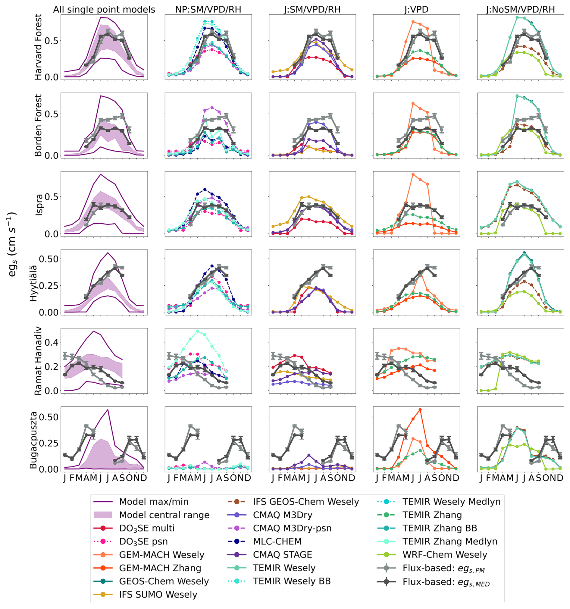
Figure 1 Monthly daytime averages of flux-based eg_s, marked as “Flux-based: eg_s,PM” and “Flux-based: eg_s,MED”, as well as single-point modeled eg_s. Column 1 shows the model central range, minimum, and maximum of monthly daytime averages of all single-point modeled eg_s. Columns 2–5 show monthly daytime averages of single-point modeled eg_s by stomatal conductance model type. NP is net photosynthesis coupled. J is Jarvis-type. SM is soil moisture, VPD is near-surface VPD, and RH can be relative humidity at the leaf surface or measurement height. Rows are labeled by site. Dots show the monthly mean eg_s, and vertical bars show ±2 standard errors of the mean.

We next compare the observed flux-based estimates, eg_s,PM and eg_s,MED, to the single-point models. In addition to the observed flux-based estimates, Fig. 1 shows the eg_s estimates from each single-point model as divided into the four classes of stomatal conductance models described in Sect. 2.1. Figure 1 also displays the central range, the maximum value, and the minimum values of the monthly averages from all single-point models. The seasonal cycle of eg_s,PM and eg_s,MED agrees with the seasonal cycle of the central range at most forest sites (Fig. 1). Specifically, monthly mean eg_s,MED and eg_s,PM estimates fall within the central range (Fig. 1) throughout times of peak GPP at Harvard Forest, Borden Forest, and Ispra during June, July, and August (Fig. S1). At Harvard Forest, Borden Forest, and Ispra, the central range suggests an increase in eg_s into the summer months (June, July, August) with declines after September. Monthly averages for eg_s,PM and eg_s,MED display the same seasonal cycle at these forest sites. Even though the seasonal cycle of eg_s suggested by the central range is supported by the flux-based averages, individual model averages can disagree with the eg_s,PM and eg_s,MED averages at these three forests (Fig. 1). For example, GEM-MACH Wesely averages show an earlier and more abrupt decline in eg_s into September after the summer months at Harvard Forest, Borden Forest, and Ispra compared to the averages from some other single-point models, eg_s,PM, and eg_s,MED.

At the boreal forest in Hyytiälä, the April–July increase in eg_s in the single-point model central range is well supported by the eg_s,MED and eg_s,PM averages (Fig. 1). However, the agreement between the central range and flux-based averages degrades past July. The flux-based estimates continue to show increasing eg_s into August, while the upper limit of the central range begins to decline past the July peak (Fig. 1). Among the forests, the largest disagreement between flux-based eg_s and the central range occurred at Hyytiälä during times of peak GPP in August and September (Figs. 1 and S1). During these months, the multiyear mean eg_s,PM and eg_s,MED are higher compared to the central range and most single-point models. GEM-MACH Wesely averages show a more rapid decline in eg_s past the June peak compared to the other single-point models at Hyytiälä. Furthermore, IFS SUMO Wesely averages suggest declining eg_s from March to December, while most other models do not show post-peak eg_s declines until after July (Fig. 1).

At the shrubland site, Ramat Hanadiv, the monthly mean eg_s,MED falls within the model central range during the winter and spring months (January–May) (Fig. 1). The central range and both eg_s,MED and eg_s,PM averages suggest declining eg_s into the dry summer months at this site. However, the central range suggests a more flat seasonal cycle in eg_s with less variability between the wet months and dry months compared to eg_s,MED and eg_s,PM. Compared to the forests examined here, there is stronger disagreement about the seasonal cycle of eg_s among individual single-point models at Ramat Hanadiv. For example, some models, such as GEM-MACH Zhang, TEMIR Zhang, GEM-MACH Wesely, WRF-Chem Wesely, and CMAQ STAGE, estimate higher eg_s during the dry summer months compared to the wet winter months, which is not supported by eg_s,MED and eg_s,PM (Fig. 1). Some single-point models like those from the TEMIR models, GEM-MACH Wesely, and WRF-Chem Wesely show rapidly increasing eg_s into the spring months (March–May), which is not supported by eg_s,MED or eg_s,PM averages. Other models like CMAQ M3Dry models, IFS SUMO Wesely, TEMIR Wesely, and IFS GEOS-Chem Wesely show relatively less month-to-month variability in eg_s compared to eg_s,MED and eg_s,PM (Fig. 1).

Out of all of the ecosystems studied here, the highest disagreement in monthly means between modeled and flux-based eg_s occurs at Bugacpuszta where data are unfortunately missing during June and July. Clifton et al. (2023) also noted this for O₃ V_d at this site. Many single-point models as well as the central range show a single and sharply peaked seasonal cycle with a maximum during June and July (Fig. 1). The limited observations at Bugacpuszta used for this activity do not allow us to confidently estimate the full seasonal cycle of flux-based eg_s at this site. Looking at the months when observations were available, eg_s,MED and eg_s,PM are higher than the central range and the maximum modeled monthly averages during most available months with the exception of May, August, and September (Fig. 1). Thus, neither the central range nor individual single-point models simulate eg_s monthly averages that are in agreement with flux-based estimates. As Clifton et al. (2023) noted, during August and September, soil volumetric water content was below the model-specified wilting point (Fig. S1) and many single-point models that include soil moisture stress simulate very low eg_s, lowering the central range. eg_s,MED and eg_s,PM also show lowered eg_s during the limited observations in August and September.

3.2 Comparison of eg_s during moisture stress: case studies at Borden Forest and Ramat Hanadiv

Figure 2 shows a comparison between single-point modeled and observed flux-based eg_s during times of observed increases in soil and atmospheric dryness. The top panel shows the comparison for Borden Forest and the bottom panel shows the comparison for Ramat Hanadiv. For Borden Forest, the purple box plot shows the distribution of (half-)hourly July eg_s during 2011 and 2012. The green box plot shows the distribution of (half-)hourly July eg_s during all years excluding 2011 and 2012. The flux-based estimates of eg_s, eg_s,PM, and eg_s,MED demonstrate that the observed decreases in soil moisture and increases in VPD_air during July 2011 and 2012 did not lower stomatal conductance or eg_s at Borden Forest (Fig. 2). Similarly, some single-point models do not show reductions in eg_s during July 2011 and 2012 compared to the July distribution of eg_s outside of 2011 and 2012 (Fig. 2). However, other single-point models show reductions in eg_s during July 2011 and 2012 that are too large (Fig. 2); these are models that use specific functions to simulate the effect of soil moisture on stomatal conductance (the NP:SM/VPD/RH and J:SM/VPD/RH models). Thus, single-point models that simulate the effect of soil moisture on stomatal conductance underestimated eg_s compared to flux-based estimates at this temperate–boreal transition forest.

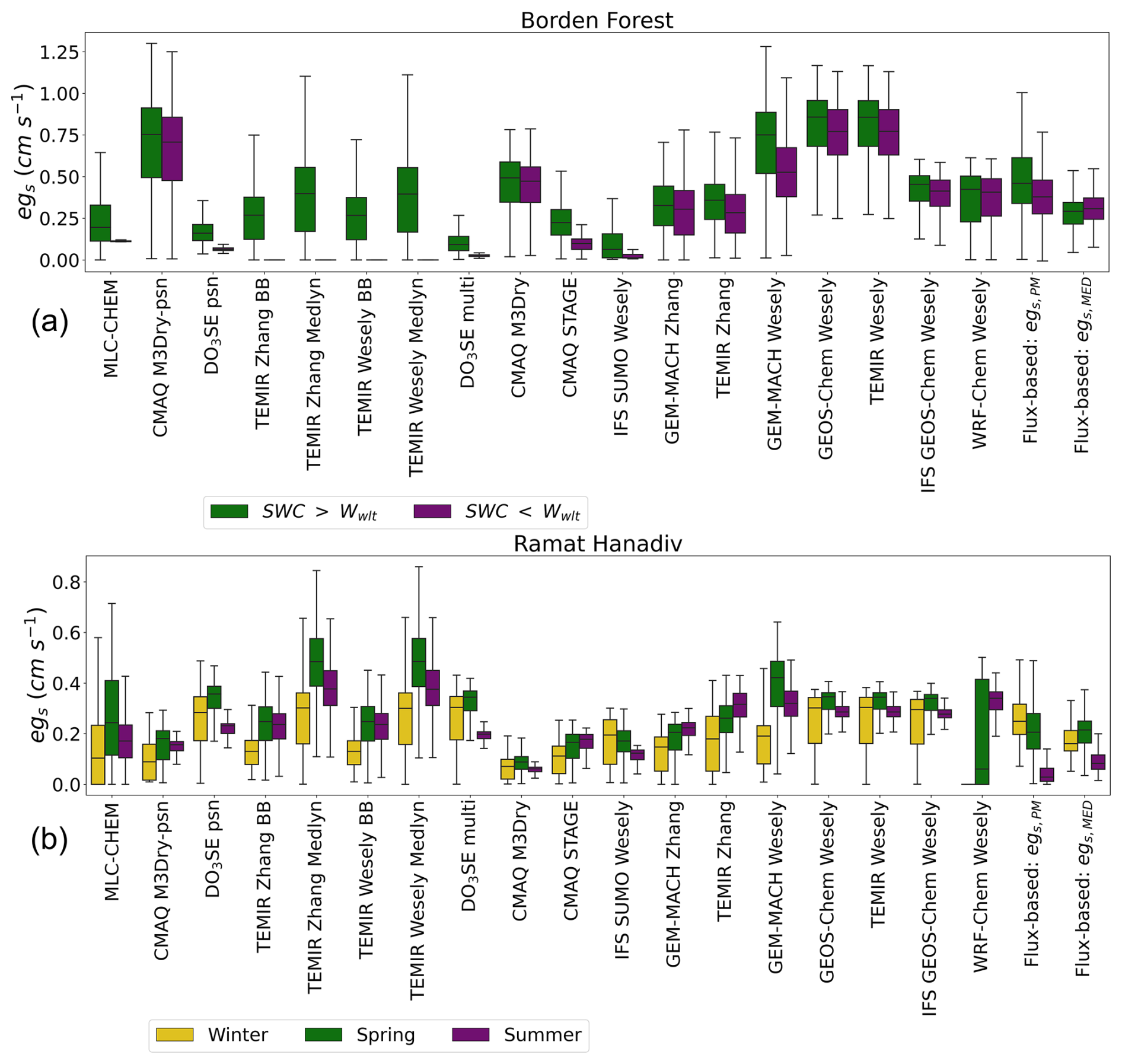
Figure 2 Comparisons of simulated eg_s and observed flux-based eg_s, “Flux-based: eg_s,PM” and “Flux-based: eg_s,MED”, for sites used in two case studies. Panel (a) shows box plots of Borden Forest for daytime, (half-)hourly July estimates during years with observed decreases in July mean soil moisture below the model wilting point (marked as “SWC <W_wlt”) compared to other years when July mean soil moisture was above the model wilting point (marked as “SWC >W_wlt”). Panel (b) shows box plots of estimates during the winter, spring, and summer at Ramat Hanadiv. The boxes display the interquartile range (IQR), with the median marked with a horizontal line inside the box. The whiskers extend to 1.5 IQR on either side of the box. Outliers were removed.

For Ramat Hanadiv, the box plots labeled “Winter” show the distribution of (half-)hourly January–February eg_s, the box plots labeled “Spring” show the distribution of (half-)hourly March–May eg_s, and the box plots labeled “Summer” show the distribution of (half-)hourly June–September eg_s. Ramat Hanadiv experienced periods of observed decreases in soil moisture and increases in VPD_air during the summer months, and the shrubland responds with decreases in observed flux-based eg_s (Fig. 2). As discussed in Sect. 3.2, individual models vary greatly in their seasonal cycles of eg_s at this site. For example, TEMIR Zhang, GEM-MACH Zhang, GEM-MACH Wesely, WRF-Chem Wesely, and CMAQ STAGE simulate the opposite seasonal cycle in eg_s compared to eg_s,PM and eg_s,MED, with higher eg_s during the dry summer months compared to the wet winter months (Fig. 2). These models that do not capture the observed seasonality in eg_s or suggest peak eg_s during the dry months at Ramat Hanadiv are Jarvis-type models that do not include specific stress functions for soil moisture stress (J:VPD or J:NoSM/VPD/RH), with the exception of CMAQ STAGE. TEMIR Zhang and GEM-MACH Zhang use a leaf water potential function to simulate moisture stress, and we find that the simulated effect is not in agreement with flux-based estimates for this shrubland. GEM-MACH Wesely and WRF-Chem Wesely use season-specific initial resistances, $R_{\mathrm{s},{\mathrm{H}}_{\mathrm{2}}\mathrm{O},\text{ideal}}$, set to very large values for winter and autumn, which is in disagreement with the seasonal cycle of flux-based stomatal conductance at this site.

The two cases presented here reveal that current model formulations of the effects of moisture stress on stomatal conductance can both over- and underestimate these effects relative to what is implied by flux-based stomatal conductance estimates. The Borden Forest case represents a case where eg_s was underestimated by many models compared to eg_s,PM and eg_s,MED when observed soil moisture fell below the model threshold determined by parameter choice. The Ramat Hanadiv case represents a case where eg_s was overestimated by many models compared to eg_s,PM and eg_s,MED during the dry summer months. Both simulated moisture stress and the seasonality of stomatal conductance through the specification of season-specific initial resistances appear to contribute to disagreement in eg_s. In the next section, we focus on the sensitivity of the agreement between single-point modeled and flux-based eg_s to changes in the values of model parameters that control: stomatal moisture stress, the relationship between net photosynthesis and stomatal conductance, and the conductance/resistance under ideal growing conditions. We discuss the sensitivity to model parameter values for all sites first and then focus on our case studies.

3.3 Moisture-stress-related parameter perturbations

The agreement between single-point modeled and flux-based eg_s is more sensitive to the choice of values for certain parameters compared to others, and certain parameters are only relevant at some sites, while other parameter values can impact agreement at all sites (Figs. 3 and S2). At all sites, the perturbation of the $G_{\mathrm{s},{\mathrm{H}}_{\mathrm{2}}\mathrm{O},\text{max}}$ parameter used to set a maximum stomatal conductance under ideal growing conditions leads to the highest change in MAD_PM and MAD_MED with a change in parameter value (Figs. 3 and S2). The agreement between single-point modeled and flux-based eg_s is sensitive to changes in B_VPD, VPD_max, f(VPD), f(RH_l), and g₁ at all sites investigated with sensitivity simulations (Figs. 3 and S2). The B_VPD parameter controls the strength of the VPD_air stress in the Jarvis-type GEM-MACH Zhang and TEMIR Zhang models. Conversely, perturbing the soil moisture stress parameters, W_wlt, ψ_soil,wlt, and B, results in substantially greater changes in MAD_PM and MAD_MED with changes in parameter values at sites that experienced substantial declines in soil moisture compared to sites that did not (Figs. 3 and S2). This indicates that the agreement between single-point modeled and flux-based eg_s is sensitive to VPD_air and RH_l moisture stress parameters and functions at all sites, while the sensitivity to soil moisture stress parameters is limited to sites that experience substantial soil moisture declines. Perturbing the values of $R_{\mathrm{s},{\mathrm{H}}_{\mathrm{2}}\mathrm{O},\text{ideal}}$ and ψ_soil,wlt results in the smallest changes in MAD_PM and MAD_MED (Figs. 3 and S2). While there were small changes in MAD_PM and MAD_MED with changes in ψ_soil,wlt within the range of ψ_soil,wlt values that were used to compute $\frac{\mathrm{\Delta }{\text{MAD}}_{\text{PM}}}{\mathrm{\Delta }v}$ and $\frac{\mathrm{\Delta }{\text{MAD}}_{\text{MED}}}{\mathrm{\Delta }v}$, perturbing the ψ_soil,wlt to a substantially lower value, $-\mathrm{1}\times {\mathrm{10}}^{\mathrm{9}}$, results in a substantial reduction of bias during our case studies, which we discuss below. Parameter perturbations that resulted in a near-zero $\frac{\mathrm{\Delta }{\text{MAD}}_{\text{PM}}}{\mathrm{\Delta }v}$ at all sites are not shown in Fig. 3.

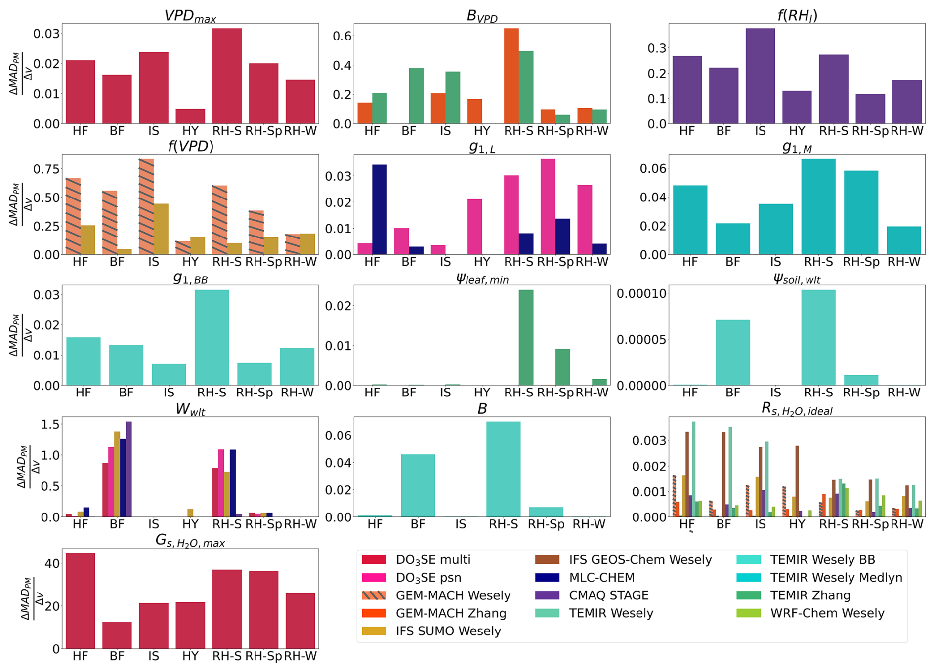
Figure 3 Comparisons of the change in median absolute difference between single-point modeled eg_s and flux-based eg_s,PM (ΔMAD_PM) with changes in a parameter or stress function value (Δv) for each parameter and stress function at each site. For each model–parameter pair or model–stress function pair, one summer $\frac{\mathrm{\Delta }{\text{MAD}}_{\text{PM}}}{\mathrm{\Delta }v}$ was calculated for Harvard Forest (HF), Borden Forest (BF), Ispra, (IS), and Hyytiälä (HY), and three $\frac{\mathrm{\Delta }{\text{MAD}}_{\text{PM}}}{\mathrm{\Delta }v}$ values were calculated for Ramat Hanadiv: winter (RH-W), spring (RH-Sp), and summer (RH-S). MAD_PM was calculated using daytime (half-)hourly estimates of eg_s.

During July 2011 and 2012 when Borden Forest experienced reductions in soil moisture without experiencing reductions in flux-based eg_s, we find that decreasing the strength of the soil moisture stress by changing the values of the wilting point in both soil volumetric water content (W_wlt) and soil matric potential (ψ_soil,wlt) results in the largest reductions in absolute values of ${\text{MD}}_{{\text{eg}}_{\mathrm{s},\text{PM}}}$ and ${\text{MD}}_{{\text{eg}}_{\mathrm{s},\text{MED}}}$ (Figs. 4 and S3) for the models that showed considerable declines in eg_s from the single-point model base simulations during July 2011 and 2012 (Fig. 2). We discuss some notable examples of reductions in absolute ${\text{MD}}_{{\text{eg}}_{\mathrm{s},\text{PM}}}$, but we keep the positive or negative sign to indicate the single-point model underestimation in the base simulations. Perturbing the wilting point resulted in a reduction in the 2011 and 2012 multiyear July ${\text{MD}}_{{\text{eg}}_{\mathrm{s},\text{PM}}}$ from 0.199 cm s⁻¹ from the base simulation for CMAQ STAGE to 0.021 cm s⁻¹ from the sensitivity simulation with the lowest ${\text{MD}}_{{\text{eg}}_{\mathrm{s},\text{PM}}}$ (Fig. 4). Perturbing the wilting point resulted in a reduction in the 2011 and 2012 multiyear July ${\text{MD}}_{{\text{eg}}_{\mathrm{s},\text{PM}}}$ from 0.236 to 0.040 cm s⁻¹ for DO₃SE psn, a reduction from 0.270 to 0.148 cm s⁻¹ for DO₃SE multi, a reduction from 0.191 to −0.008 cm s⁻¹ for MLC-CHEM, a reduction from 0.295 to −0.083 cm s⁻¹ for TEMIR Wesely BB, and a reduction from 0.273 to −0.095 cm s⁻¹ for IFS SUMO Wesely (Fig. 4).

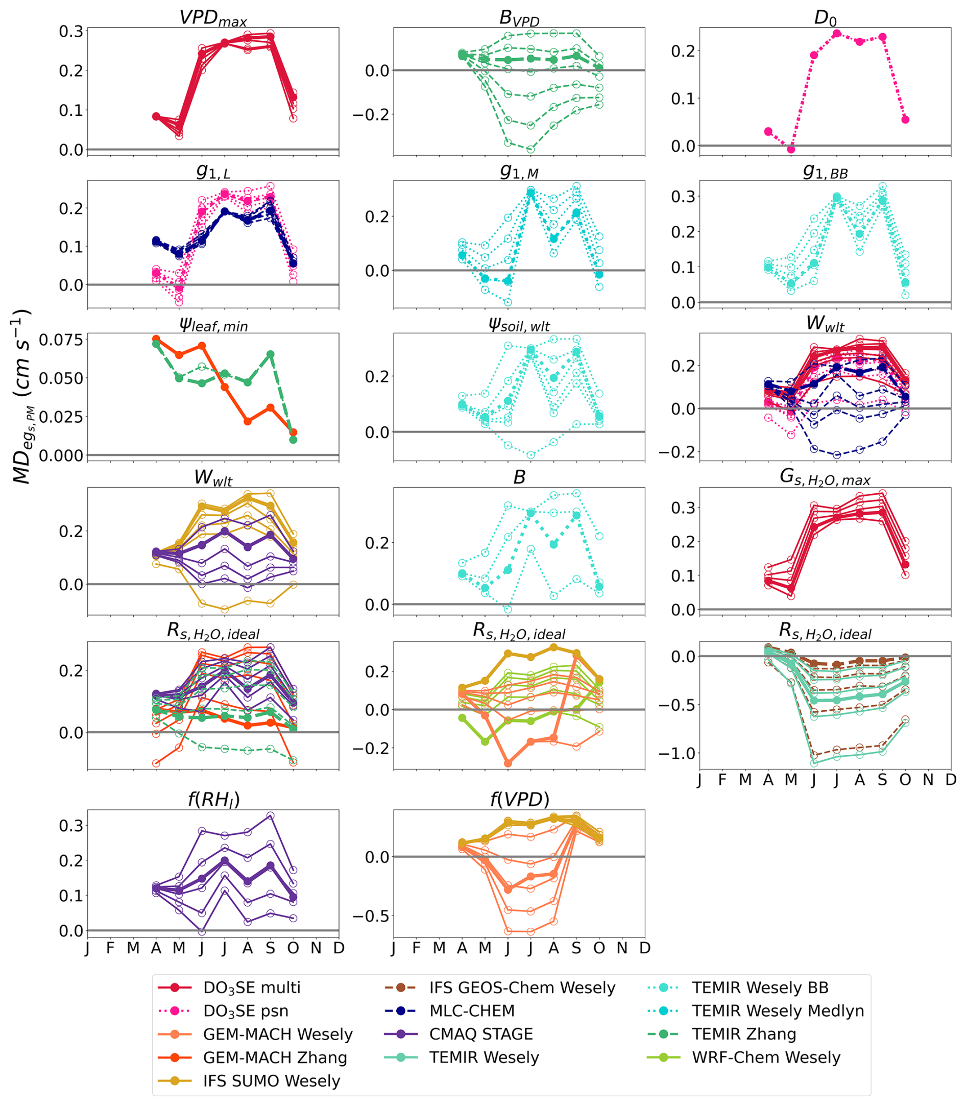
Figure 4 The 2011 and 2012 multiyear monthly median difference between single-point modeled eg_s and observed flux-based eg_s,PM (${\text{MD}}_{{\text{eg}}_{\mathrm{s},\text{PM}}}$) at Borden Forest for base and sensitivity simulations of single-point models. Sensitivity simulations perturbed the values of each parameter and stress function. Lines with filled dots show the ${\text{MD}}_{{\text{eg}}_{\mathrm{s},\text{PM}}}$ for base simulations of single-point models. Lines with open dots show the ${\text{MD}}_{{\text{eg}}_{\mathrm{s},\text{PM}}}$ for each parameter or stress function perturbation where each line represents one perturbation. Table 2 lists the interpretation of the parameters, stress functions, and values used for sensitivity simulations. W_wlt and $R_{\mathrm{s},{\mathrm{H}}_{\mathrm{2}}\mathrm{O},\text{ideal}}$ are shared among many models, and they are displayed in multiple plots to avoid plotting many model results in a single plot.

For the second case study at Ramat Hanadiv, we find that MAD_PM and MAD_MED were the most sensitive during the dry summer months to the values of most of the parameters we studied (Figs. 3 and S2). Increasing the strength of the soil moisture stress through changes in the ψ_soil,wlt and B parameters and increasing the strength of the VPD_air and RH stress through changes in the B_VPD parameter and the f(VPD) and f(RH_l) stress functions resulted in large reductions in absolute ${\text{MD}}_{{\text{eg}}_{\mathrm{s},\text{PM}}}$ and ${\text{MD}}_{{\text{eg}}_{\mathrm{s},\text{MED}}}$ during the dry summer months (Figs. 5 and S4). For most net photosynthesis coupled models, changing the g₁ parameter also resulted in reductions in absolute ${\text{MD}}_{{\text{eg}}_{\mathrm{s},\text{PM}}}$ and ${\text{MD}}_{{\text{eg}}_{\mathrm{s},\text{MED}}}$ during the dry season (Figs. 5 and S4). We focus on July to discuss notable examples of the reductions in absolute ${\text{MD}}_{{\text{eg}}_{\mathrm{s},\text{PM}}}$ from the base simulations to the sensitivity simulations, but again, we keep the positive or negative sign to indicate the single-point model overestimation in the base simulations.

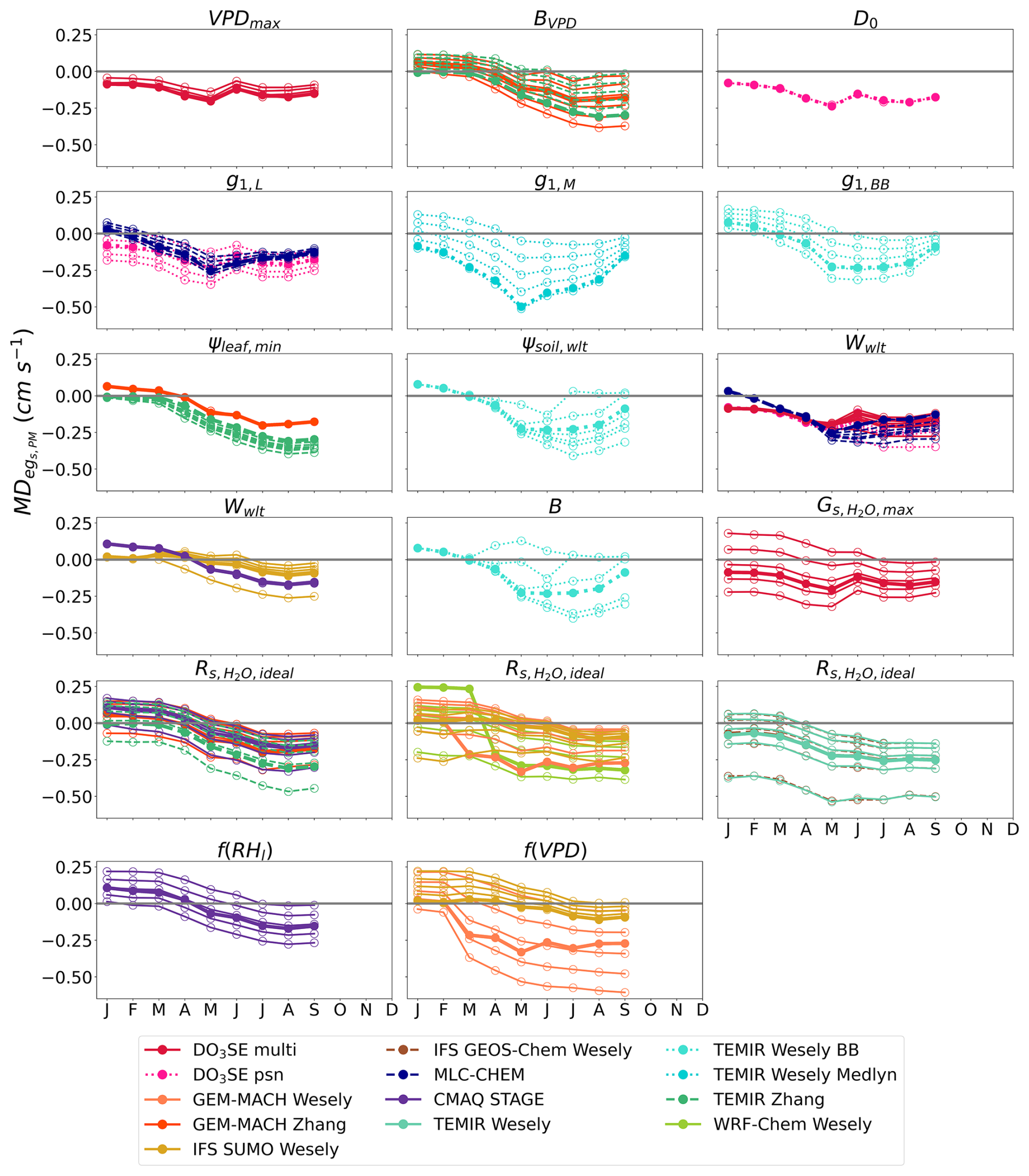
Figure 5 Monthly median difference between single-point modeled eg_s and observed flux-based eg_s,PM (${\text{MD}}_{{\text{eg}}_{\mathrm{s},\text{PM}}}$) at Ramat Hanadiv for base and sensitivity simulations of single-point models. Some months have multiple years of data. Sensitivity simulations perturbed the values of each parameter and stress function. Lines with filled dots show the ${\text{MD}}_{{\text{eg}}_{\mathrm{s},\text{PM}}}$ for base simulations of single-point models. Lines with open dots show the ${\text{MD}}_{{\text{eg}}_{\mathrm{s},\text{PM}}}$ for each parameter or stress function perturbation where each line represents one perturbation. Table 2 lists the interpretation of the parameters, stress functions, and values used for sensitivity simulations. W_wlt and $R_{\mathrm{s},{\mathrm{H}}_{\mathrm{2}}\mathrm{O},\text{ideal}}$ are shared among many models, and they are displayed in multiple plots to avoid plotting many model results in a single plot.

Perturbing the ψ_soil,wlt and B parameters resulted in an ${\text{MD}}_{{\text{eg}}_{\mathrm{s},\text{PM}}}$ reduction from −0.228 to 0.030 cm s⁻¹ for TEMIR Wesely BB (Fig. 5). Perturbing the B_VPD parameter resulted in an ${\text{MD}}_{{\text{eg}}_{\mathrm{s},\text{PM}}}$ reduction from −0.276 to −0.054 cm s⁻¹ for TEMIR Zhang and a reduction from −0.202 to −0.067 cm s⁻¹ for GEM-MACH Zhang (Fig. 5). For GEM-MACH Wesely, both the f(VPD) stress function and the $R_{\mathrm{s},{\mathrm{H}}_{\mathrm{2}}\mathrm{O},\text{ideal}}$ parameter resulted in large reductions in ${\text{MD}}_{{\text{eg}}_{\mathrm{s},\text{PM}}}$ and ${\text{MD}}_{{\text{eg}}_{\mathrm{s},\text{MED}}}$ (Figs. 5 and S4). Perturbing the f(VPD) stress function resulted in an ${\text{MD}}_{{\text{eg}}_{\mathrm{s},\text{PM}}}$ reduction from −0.305 to −0.037 cm s⁻¹, and perturbing the $R_{\mathrm{s},{\mathrm{H}}_{\mathrm{2}}\mathrm{O},\text{ideal}}$ parameter resulted in a reduction in ${\text{MD}}_{{\text{eg}}_{\mathrm{s},\text{PM}}}$ from −0.305 to −0.043 cm s⁻¹ for GEM-MACH Wesely. Perturbing the f(RH_l) stress function resulted in an ${\text{MD}}_{{\text{eg}}_{\mathrm{s},\text{PM}}}$ reduction from −0.152 to −0.003 cm s⁻¹ for CMAQ STAGE. Perturbing the g_1,BB parameter resulted in an ${\text{MD}}_{{\text{eg}}_{\mathrm{s},\text{PM}}}$ reduction from −0.228 to −0.046 cm s⁻¹ for TEMIR Wesely BB (Fig. 5). Perturbing the g_1,M parameter resulted in an ${\text{MD}}_{{\text{eg}}_{\mathrm{s},\text{PM}}}$ reduction from −0.372 to −0.077 cm s⁻¹ for TEMIR Wesely Medlyn (Fig. 5).

4 Discussion

After comparing the single-point simulated stomatal component of O₃ V_d from various dry deposition schemes implemented in 3D atmospheric chemistry models with inversion-based estimates using observed λE and CO₂ flux, we find that the agreement between single-point modeled and flux-based eg_s is sensitive to the specification of moisture stress on stomatal conductance. This is evident in both over- and underestimating the strength of stomatal moisture stress depending on the ecosystem. When comparing agreement between simulated eg_s and flux-based eg_s across the four stomatal conductance model types described in Sect. 2.1, there is no conclusive evidence that all models within one class of stomatal conductance models are always in higher agreement with flux-based eg_s at all ecosystems in the study. For example, the maximum monthly average among models is shaped by the higher eg_s values from the Jarvis-type models without soil moisture, VPD, or RH stress (J:NoSM/VPD/RH) at the forest sites during June, July, and August. However, at Ramat Handiv, a single model from the net photosynthesis coupled class of models defines the model maximum monthly average. Furthermore, the model minimum averages are defined by models that do include moisture stress. The study does suggest that improved process representation of moisture stress is beneficial for agreement across different ecosystems. For example, one can expect agreement in seasonality between simulated eg_s and observed flux-based eg_s using models in all four stomatal conductance model classes at sites like Borden Forest, Harvard Forest, and Ispra where plant productivity is highest in the summer months. However, parameterizations in all models lacking soil moisture stress led to drastic disagreements in a seasonally dry ecosystem like Ramat Hanadiv where the vegetation activity is highest during the rainy winter months and stomatal conductance substantially declines during summer months due to water stress. Not all but many models that have increased representation of water stress achieve better agreement with observed flux-based estimates at Ramat Hanadiv. In general, the increased representation of moisture stress and refining moisture-stress-related parameter values allow certain models to agree better with observation-based estimates across a variety of ecosystems. We further discuss the two case studies: (1) Borden Forest, a temperate–boreal transition forest where observed declines in soil moisture did not limit the GPP, λE, and stomatal conductance, and (2) Ramat Hanadiv, an eastern Mediterranean shrubland where the local vegetation is adapted to seasonal declines in soil moisture (Vænänen et al., 2020). Finally, we discuss the divergence between the flux-based estimates that we found at these two sites.

4.1 Moisture stress for stomatal conductance at a northern boreal–temperate transition forest

The case studies of observed declines in soil moisture at 50 cm depth at Borden Forest suggest that many single-point models struggle to capture the observed flux-based response of stomatal conductance during these conditions, resulting in disagreements in eg_s. Long-term observations suggest that summertime net ecosystem productivity at Borden Forest is more strongly controlled by photosynthetically active radiation, air temperature, and soil temperature rather than soil moisture or VPD_air (Froelich et al., 2015). High air and soil temperatures, along with high photosynthetically active radiation during the summer months, coincide with the highest net ecosystem productivity (Froelich et al., 2015). July 2011 and 2012 were months with observed declines in soil moisture at 50 cm depth in this study, but interannually, 2011 and 2012 were also the years with the highest shortwave radiation and GPP at Borden Forest during the summer months (Fig. S1).

This suggests that the observed decline in soil moisture at 50 cm depth does not limit stomatal conductance. Previous analysis of long-term CO₂ exchange data from Borden Forest from 1996–2013 showed that the only year when the drops in soil moisture and precipitation were severe enough to create noticeable declines in GPP was 2007 (Froelich et al., 2015). This indicates that while the wilting point specified for 50 cm depth in some single-point models estimated the lowest eg_s during July 2011 and 2012 at Borden Forest, the observed flux-based estimates of stomatal conductance and previous longer-term estimates of GPP do not consider 2011 and 2012 to be years of vegetation water stress in terms of reductions in GPP. A wilting point specified for measurements of soil moisture at 50 cm depth might not reflect the soil water sources that are available to the trees at Borden Forest where red maples (Acer rubrum) can make up 50 % of the tree species composition (Teklemariam et al., 2009). At the Hubbard Brook Experimental Forest (HBEF) in the northeastern US, red maples primarily used shallow soil water sources at less than 10 cm depth during June 2018 and less than 30 cm depth during July 2018 (Harrison et al., 2020). However, their primary source of soil water shifted to depths of 90–100 cm in August, suggesting that red maples can switch the depths from which they access soil water within a growing season (Harrison et al., 2020). Seasonal adjustments in tree water uptake depths have been widely observed (Bachofen et al., 2024), and the possibility of similar dynamics in tree access to soil water at Borden Forest makes it challenging to apply wilting point type thresholds at a single measurement depth for point models. Disagreements between single-point modeled and observed flux-based eg_s suggest that simulating the effects of soil moisture on stomatal conductance for a northern boreal–temperate transition forest can benefit from incorporating tree access to variable soil water sources.

4.2 Moisture stress for stomatal conductance for a seasonally dry eastern Mediterranean shrubland

There can be significant interspecific variation in net photosynthesis, transpiration, and stomatal conductance among the co-existing woody species at Ramat Hanadiv during the dry summer months due to varying drought resistance between the species (Vænänen et al., 2020). Native woody species at this shrubland like Quercus calliprinos employ a host of resistance strategies and likely exhibit greater rooting depth and access to deep water reserves to withstand seasonal declines in soil moisture (Väänänen et al., 2020). The leaf-level stomatal conductance of the woody species declines during the dry summer months with increases in VPD_air and decreases in soil moisture (Vænänen et al., 2020). Our flux-based estimates of eg_s and previous flux-based estimates in the region also confirm that the vegetation at Ramat Hanadiv and other regional sites experiences declines in stomatal conductance into the dry summer months as soil moisture declines and VPD_air increases (Li et al., 2018, 2019).

Many single-point models simulated increasing eg_s into the dry months. These models include those that simulate the effects of both soil moisture and VPD_air or RH_l, those that simulate the effects of VPD_air and leaf water potential, and those that do not simulate the effects of moisture stress on stomatal conductance. Increasing the RH_l and VPD stress through parameter and stress function perturbations increased the summertime agreement between single-point modeled and flux-based eg_s for models that simulated increasing eg_s into summer. Some single-point models that simulate increasing eg_s into the dry months prescribe a seasonally varying $R_{\mathrm{s},{\mathrm{H}}_{\mathrm{2}}\mathrm{O},\text{ideal}}$. The high wintertime and low summertime $R_{\mathrm{s},{\mathrm{H}}_{\mathrm{2}}\mathrm{O},\text{ideal}}$ in these models, based on temperate ecosystems, likely contributes to disagreements in the seasonality of eg_s with other models and flux-based estimates. Finally, the models that simulate the effects of leaf water potential on stomatal conductance without simulating the effects of soil water potential also simulated increasing eg_s into the dry summer months. Leaf water potential is simulated to vary only as a function of shortwave radiation (Clifton et al., 2023). However, leaf water potential is mechanistically coupled with soil water potential, although the relationship between the two can vary due to plant water regulation (Sack and Holbrook, 2006; Martínez Vilalta et al., 2014; Venturas et al., 2017). The leaf water potential of woody species at Ramat Hanadiv has shown strong linear relationships with soil water potential (Vænänen et al., 2020). Coupling the simulation of leaf water potential with the simulation of soil water potential in these models presents an opportunity to improve stomatal conductance and by extension eg_s sensitivity to drought.

4.3 Comparison of available methods to estimate the stomatal component of O₃ dry deposition from observed latent heat and CO₂ flux

We found that individual eg_s estimates calculated from inversion and observed flux-based methods can exhibit disagreements in two ecosystems. For example, eg_s estimates from a Penman–Monteith inversion using latent heat flux can disagree in eg_s from fitting an optimality-based stomatal conductance model using GPP partitioned from NEE at Borden Forest. We also found disagreements in magnitude between the two methods to infer stomatal conductance at Ramat Hanadiv. The source of this disagreement is the difference in the underlying flux used to calculate the stomatal conductance estimate and the dependence of conductance on VPD in the method used. At all sites, $G_{\mathrm{s},{\mathrm{H}}_{\mathrm{2}}\mathrm{O},\text{MED}}$ had a higher dependence on GPP and NEE compared to the dependence of $G_{\mathrm{s},{\mathrm{H}}_{\mathrm{2}}\mathrm{O},\text{PM}}$ estimates on latent heat flux used in the Penman–Monteith inversion.

The dependence of stomatal conductance on VPD_canopy-air indicated that at low VPD_canopy-air, higher stomatal conductance was estimated from a PM inversion compared to upscaling the Medlyn et al. (2011) model using GPP. This could explain the disagreements at Borden Forest between the two flux-based estimates. It is important to note that we used the nighttime method to partition NEE into GPP and R_eco to avoid the added dependence of GPP on near-surface VPD that the daytime method introduces (Lasslop et al., 2010) considering the Medlyn et al. (2011) model also includes the effects of VPD_canopy-air. Regardless of the varying degrees of dependence on VPD that single-point models and flux-based estimates can display, the two major findings from the two case studies at Borden Forest and Ramat Hanadiv hold. At Ramat Hanadiv, using both GPP and latent heat flux to estimate stomatal conductance shows a decline of eg_s into the dry summer months, which is confirmed by previous leaf-level gas exchange measurements at the site. Furthermore, both flux-based estimates of eg_s do not suggest a substantial decline in eg_s simulated by single-point models during July 2011 and 2012 at Borden Forest.

5 Conclusions

Simulating the dry deposition of O₃ to the land surface is a crucial component of simulating O₃ concentrations and air quality. Here, we compared estimates from various dry deposition schemes implemented in chemical transport models run as single-point models forced with observed micro-meteorology and environmental conditions at flux tower sites. Specifically, we focused on comparing observed flux-based estimates of the stomatal component of O₃ dry deposition, eg_s, with simulations of eg_s by the single-point models by aiming to answer three research questions.

1. How does the stomatal component of O₃ deposition velocity from single-point models compare with the estimates from observed latent heat and CO₂ flux?

2. How does the specification of moisture stress in single-point models impact the agreement in the stomatal component of O₃ deposition velocity between single-point model simulations and flux-based estimates during times of increased atmospheric or soil dryness?

3. In dry deposition schemes, how do stomatal moisture stress parameters affect the agreement between single-point models and observed flux-based estimates?

To answer question 1, we find that monthly mean observed flux-based eg_s agrees with a central ensemble range of monthly mean eg_s by single-point model simulations during parts of the growing season at all sites when multiyear data were available. However, when we focused on specific cases of increased atmospheric or soil dryness within the observational dataset, we found that moisture stress specification resulted in disagreements between single-point modeled and flux-based eg_s. To answer question 2, we find that single-point modeled soil moisture stress for stomatal conductance was too strong in a light- and temperature-limited northern temperate–boreal transition forest where high summertime photosynthetically active radiation and temperatures favor high net ecosystem productivity and the tree species likely have access to deeper soil water sources compared to the depth at which the soil moisture was measured. This resulted in underestimation of eg_s by some single-point models compared to observed flux-based estimates because observed soil moisture at 50 cm depth fell below the model-specified wilting point. Furthermore, an eastern Mediterranean shrubland where seasonality in stomatal conductance is driven by water availability is poorly represented by some single-point models. Many single-point models overestimated eg_s compared to observed flux-based estimates during the dry summer months.

To answer question 3, we find that at all sites examined, single-point modeled eg_s and the agreement with observed flux-based eg_s were sensitive to parameters that control the vapor pressure deficit stress and the relationship between net photosynthesis and stomatal conductance. Conversely, the simulation of eg_s and the agreement with observed flux-based eg_s were highly sensitive to parameters that control the soil moisture stress only at specific sites that experienced substantial declines in soil moisture. This suggests that the simulated eg_s is highly sensitive to parameter choice for soil moisture stress when environmental conditions start to reach model thresholds like the wilting point, leading to large disagreements between single-point modeled and flux-based eg_s. Clifton et al. (2023) showed that stomatal conductance is the most important driver of the seasonal variability in simulated deposition velocity in many of the single-point models at all of the sites in this study. Thus, the simulations of stomatal conductance will directly impact total deposition velocity among these models. This indicates that the impacts of simulating stomatal moisture stress on stomatal conductance and eg_s estimates shown here could likely propagate to O₃ deposition velocity.

In order to simulate O₃ dry deposition in the face of projected increases in aridity, understanding and correctly parameterizing the response of stomatal conductance to decreases in soil moisture and increased vapor pressure deficit across a range of ecosystems will play a key role in improving the simulation of O₃ dry deposition during drought conditions. Other beneficial model developments could include simulating the impact of O₃ on stomatal conductance. O₃ uptake itself can impact stomatal conductance and its response to other environmental conditions like soil moisture. Using results from chamber and free-air exposure studies, various methods to incorporate O₃ effects on stomata such as developing separate O₃ stress functions for the Jarvis-type models and introducing O₃ factors developed from control to treatment response ratios to net photosynthesis coupled models have been introduced (Lombardozzi et al., 2012a, 2015; Hoshika et al., 2020, 2015, 2018; Oliver et al., 2018). Ongoing developments in land surface modeling of stomatal conductance and vegetation responses to water stress will likely benefit components of tropospheric O₃ modeling.