Technical note: Towards atmospheric compound identification in chemical ionization mass spectrometry with pesticide standards and machine learning

Chemical ionization mass spectrometry (CIMS) is widely used in atmospheric chemistry studies. However, due to the complex interactions between reagent ions and target compounds, chemical understanding remains limited and compound identification difficult. In this study, we apply machine learning to a reference dataset of pesticides in two standard solutions to build a model that can provide insights from CIMS analyses in atmospheric science. The CIMS measurements were performed with an Orbitrap mass spectrometer coupled to a thermal desorption multi-scheme chemical ionization inlet unit (TD-MION-MS) with both negative and positive ionization modes utilizing Br⁻, ${\mathrm{O}}_{\mathrm{2}}^{-}$, H₃O⁺ and (CH₃)₂COH⁺ (AceH⁺) as reagent ions. We then trained two machine learning methods on these data: (1) random forest (RF) for classifying if a pesticide can be detected with CIMS and (2) kernel ridge regression (KRR) for predicting the expected CIMS signals. We compared their performance on five different representations of the molecular structure: the topological fingerprint (TopFP), the molecular access system keys (MACCS), a custom descriptor based on standard molecular properties (RDKitPROP), the Coulomb matrix (CM) and the many-body tensor representation (MBTR). The results indicate that MACCS outperforms the other descriptors. Our best classification model reaches a prediction accuracy of 0.85 ± 0.02 and a receiver operating characteristic curve area of 0.91 ± 0.01. Our best regression model reaches an accuracy of 0.44 ± 0.03 logarithmic units of the signal intensity. Subsequent feature importance analysis of the classifiers reveals that the most important sub-structures are NH and OH for the negative ionization schemes and nitrogen-containing groups for the positive ionization schemes.

1 Introduction

Mass spectrometry is an analytical technique for molecular compound identification and tracking in a variety of fields (e.g., biochemistry, food control, forensic science, pollution control, reaction physics and kinetics, thermodynamic parameters' determination) (Griffiths and de Hoffmann, 2007). In atmospheric science, chemical ionization mass spectrometry (CIMS) has proliferated because it can detect gas-phase compounds at atmospheric pressures (Sipilä et al., 2016; Laskin et al., 2018; Huey, 2007; Eisele and Tanner, 1993; Munson, 1971; Munson and Field, 1966; Riva et al., 2019; Breitenlechner et al., 2017; de Gouw and Warneke, 2007). CIMS' low detection limit, good sensitivity, low probability of fragmentation and ability to detect charged volatile compounds make it an ideal compound tracking technique. In proton-transfer-reaction mass spectrometry, properties like proton affinity are utilized to determine the detectability of compounds. Although this instrument is commonly used to quantify volatile organic precursor molecules at relatively high concentrations, more selective and sensitive techniques are typically required for analyzing highly functionalized aerosol precursors (e.g., ${\mathrm{NO}}_{\mathrm{3}}^{-}$ or I⁻; Lee et al., 2014; Rissanen et al., 2014). Multi-scheme chemical ionization inlets (MIONs) (Rissanen et al., 2019) provide more information than single ionization schemes. However, compound identification remains challenging, as our understanding of the complex interaction between reagent ions and sample molecules is still too limited to routinely identify compounds from CIMS spectra (Munson, 2006; Sandström et al., 2024).

To improve compound identification, quantum chemical calculations are used to model the interaction between reagent ions and target molecules. Early breakthroughs revealed a correlation between the binding energy (between reagent ion and target molecule) and the experimental detection sensitivity (Partovi et al., 2023, 2024; Iyer et al., 2016; Hyttinen et al., 2018). However, due to the high complexity of the interaction, the large configuration space of possible ion–molecule structures and the cost of the quantum chemical calculations, databases are challenging to produce. Thus no compound identification workflow has emerged so far.

In this article, we explore if purely data-driven machine learning (ML) can facilitate CIMS compound identification. ML excels at pattern identification, data-driven classification and regression tasks. ML is proliferating in the natural sciences and has started to emerge in atmospheric science for, e.g., physicochemical property prediction and characterization of compounds (Lumiaro et al., 2021; Sandström et al., 2024; Besel et al., 2023, 2024; Hyttinen et al., 2022, 2024; Franklin et al., 2022), detection of new particle formation events (Su et al., 2022), boundary layer height estimation (Krishnamurthy et al., 2021), or aerosol classification (Siomos et al., 2020). In other chemical domains, e.g., metabolomics, ML has successfully enabled chemical compound identification from fragmentation mass spectrometry (Erban et al., 2019; Heinonen et al., 2012; Dührkop et al., 2015; Brouard et al., 2016; Nguyen et al., 2018, 2019). The advantage of an ML-based method is twofold: it is computationally inexpensive, especially when compared to quantum chemical calculations, and it can interpolate predictions to novel compounds without requiring extensive reference data once trained. This is essential for atmospheric chemistry, where thousands of large, highly oxidized organic compounds lack reference datasets. In the short term, our method could accelerate CIMS experimental optimization and aid in reagent ion selection. However, successful identification requires comprehensive collections of reference spectra, which are needed both for traditional spectral comparison and for training ML-based methods. Currently, a lack of data standards in atmospheric science hinders similar ML advancements for CIMS and fragmentation mass spectrometry (Sandström et al., 2024; Thoma et al., 2022).

In this work, we address the scarcity of atmospheric compound data standards by testing our methodology on a reference dataset of approximately 700 pesticides measured with CIMS. While pesticides represent only a small subset of atmospheric compounds (Brüggemann et al., 2024; Houde et al., 2019), they are chemically complex, with diverse molecular masses and functional groups that can interact in distinct ways with various reagent ions and that cover an extended range of detection with CIMS. This structural diversity provides a relevant test case that reaches and surpasses the complexity of many atmospheric compounds, allowing for an effective initial test of our methodology. Additionally, pesticides are readily available as standard chemicals from chemical suppliers at an accessible cost, and the dataset size is comparable to those used to establish early ML compound identification tools in metabolomics (Heinonen et al., 2012; Dührkop et al., 2015; Brouard et al., 2016; Nguyen et al., 2018, 2019). Thus, while limited to pesticides, this dataset offers a valuable preliminary benchmark for developing ML-based CIMS signal prediction. Once reference datasets for atmospheric compounds become available, this methodology can be directly applied or refined to encompass a broader range of atmospheric chemical analyses.

Our objective in this work is to develop ML models that learn the relation between CIMS spectra and their corresponding compounds. Specifically, we will investigate if we can predict a pesticide detection by CIMS and, further, if we can predict the resulting signal intensity of different ionization methods from the molecular structure of a pesticide. Such predictions could be used prior to deployment (e.g., in a field measurement campaign or for pesticide detection and monitoring) to ensure that the detector is appropriate and sensitive enough. The ML methods will also provide insight into the interaction between reagent ions and molecules, which will help us to develop future compound identification methods in atmospheric science.

Figure 1 Schematic of the machine learning workflow followed in this work: the sample is analyzed, and the two targets of our analyses are defined. The preprocessing includes the filtering of the data and the creation of the molecular descriptors which will be fed into the ML algorithms. The two ML models are divided into classification (to predict whether a molecule is detected or not) and regression (to predict the CIMS sensitivity of a molecule). The performances of the models are evaluated, and chemical insight is extracted from the feature analysis.

Figure 1 presents the schematic ML workflow followed in this work. The measurements were carried out with a thermal desorption (TD) MION-MS, and the experiments were run sequentially with four different ionization schemes: Br⁻, ${\mathrm{O}}_{\mathrm{2}}^{-}$, H₃O⁺ and (CH₃)₂COH⁺ (AceH⁺). The dataset is then preprocessed and used for training two ML algorithms: random forest (RF) (Breiman, 2001) for detection classification and a kernel ridge regression (KRR) (Rupp, 2015) models to predict CIMS signal intensities of a given pesticide. The models are trained on molecular descriptors, which are mathematical transformations of the molecular structure that make it suitable for data-driven analysis. Different descriptors are tested and compared for both classification and regression, as each molecular representation encodes unique structural or chemical features and varies in complexity and interpretability. We tested five different representations: properties obtained from the pesticides' structure (RDKitPROP), the topological fingerprint (TopFP) (James et al., 1995), the molecular access system keys (MACCS) (Durant et al., 2002), the Coulomb matrix (CM) (Rupp et al., 2012) and the many-body tensor representation (MBTR) (Huo and Rupp, 2022). Using this range of molecular representations and data from diverse ionization schemes, we evaluate the models' ability to predict CIMS detection and signal intensity of the compounds, providing insights into how structural characteristics influence CIMS sensitivity across different ionization methods.

The paper is organized as follows: Sect. 2 presents the dataset used in this work. Sections 3 and 4 introduce the molecular descriptors and ML methodology, respectively. Section 5 presents the results of the classification (Sect. 5.1) and regression (Sect. 5.2) models, as well as a discussion on the chemical insight gained from the ML models (Sect. 5.3).

2 Dataset

Our dataset is generated from two standard mixtures received from GALAB (2025) Laboratories, containing 404 and 312 organic pesticides. The CIMS experiments were conducted at Karsa Oy laboratory (Karsa, 2025) with a TD-MION inlet operating at atmospheric pressure coupled to a linear trap quadrupole Orbitrap mass spectrometer. A sample was placed on a custom-made filter (Karsa, 2025) and heated in the desorber from 30 to 250 °C; different pesticides evaporate from the filter at various temperatures. A schematic of the instrument as well as the sampling methodology is presented in Partovi et al. (2023, 2024). The mixtures were individually measured at five different concentrations, but for this work, only measurements at the highest concentration (2.5 ng µL⁻¹) were considered. The measurements from the two mixtures were combined into a single dataset for a total of 716 pesticide observations, where each observation corresponds to the parent ion's signal intensity. Due to CIMS' soft ionization, the parent ion is expected to have the highest intensity, quantitatively, and qualitatively provides a one-to-one correspondence to the target compound. Each pesticide was measured with the following ionization schemes: bromide (Br⁻) ionization (produced from dibromomethane, CH₂Br₂), protonated acetone ((CH₃)₂COH⁺, AceH⁺) ionization (produced from acetone, (CH₃)₂CO), proton-transfer (H⁺) ionization by hydronium ions (H₃O⁺, produced from trace amounts of water, H₂O⁺) and electron transfer (–) ionization by dioxide (${\mathrm{O}}_{\mathrm{2}}^{-}$). The first two ions were obtained by feeding the neutral reagents into the ion source, while the two latter ions were obtained by feeding dopant-free air instead. The pesticides were detected as protonated ions (AceH⁺, H₃O⁺), as deprotonated ions (${\mathrm{O}}_{\mathrm{2}}^{-}$) or as adduct ions (Br⁻).

From the 716 measured pesticides, we removed 23 from the dataset (Fig. S3, Tables S1 and S2 in the Supplement) for the following reasons. A total of 12 instances correspond to six pesticides that appeared twice (once in each mixture) but were measured with different signal intensities. Next, we excluded 10 pesticides with a molecular weight outside the ideal mass spectrometer transmission window, i.e., lower than 120 u​​​​​​​ and higher than 600 u, which suffered from the corresponding significant signal loss. Another pesticide was excluded due to its out-of-range Br⁻ intensity value. Several isomers are present in the dataset (e.g., prometryn and terbutryn or phoxim and quinalphos). Across 38 molecular formulas, there are 81 isomers in total. In CIMS, isomers produce peaks at the same mass-to-charge ratio and cannot be distinguished with a single ionization method, as they can in, e.g., fragmentation mass spectrometry. To retain dataset size, we included all isomers, assigning the same signal intensity to each if detected by an ionization method and labeling all as undetected if no signal was present. This approach adds uncertainty to the ML model; can affect the evaluated model performance, depending on the structural difference of the isomers; and can limit the model validity for real-world applications requiring isomer distinction. This tradeoff allows for a larger dataset but reduces predictive accuracy at the structural level. In the following, dataset refers to the 693 pesticides remaining after removing the aforementioned 23 pesticides.

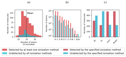
Figure 2 Distribution of (a) heavy atoms, (b) element types in logarithmic scale and (c) detection rate of the four reagent ions (Br⁻, ${\mathrm{O}}_{\mathrm{2}}^{-}$, H₃O⁺ and AceH⁺). Detected pesticides are shown in red and undetected pesticides in light blue. In panels (a) and (b), a molecule is considered detected if at least one ionization method presents a signal (full color). In panel (c) the detection status is determined per ionization method individually (striped color).

Figure 2 presents basic dataset statistics (molecular size, element composition and detection by ionization method). In Fig. 2a and b, we distinguish between detected, when a molecule presents a signal with at least one ionization method, and undetected otherwise. In Fig. 2c, detected refers to when a molecule presents a signal for a specified ionization method and undetected otherwise. The number of non-hydrogen atoms per molecule (Fig. 2a) is normally distributed for detected and undetected pesticides with an average of 20 atoms per pesticide (dashed vertical line). The smallest molecule, methamidophos, contains 7 atoms, while the largest one, acrinathrin, contains 38 atoms. In total, we find 572 pesticides, for which at least one ionization method gives a signal, and 121 undetected pesticides, for which no ionization method triggers.

Figure 2b shows a histogram of the chemical elements present in the dataset. The pesticides in our dataset are organic molecules and therefore have a prevalence for hydrogen, carbon, nitrogen and oxygen. In addition, chlorine, fluorine, sulfur and phosphorus are present in over a hundred pesticides, whereas bromine, iodine, silicon and tin occur less frequently. Tin is the only element present only in undetected molecules (Table S3 in the Supplement presents a list of tin compounds).

In Fig. 2c the total count of detected and undetected pesticides for each ionization method is shown. Differing from Fig. 2a, where a large number of pesticides appear to be detected, Fig. 2c reveals that in contrast to the positive reagent ions, the two negative reagent ions exhibit a higher number of undetected molecules than detected ones. Most pesticides are detected with AceH⁺ and fewest with ${\mathrm{O}}_{\mathrm{2}}^{-}$. The figure highlights that, for this specific dataset, negative reagent ions are more selective than positive ones for the detection of parent ions.

Table 1 Example of the chemical diversity of the dataset.

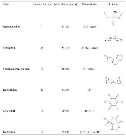
Table 1 presents six examples of chemical diversity in our dataset. The first two entries correspond to the smallest and the largest pesticides (methamidophos (7 atoms) and acrinathrin (38 atoms)). Subsequent entries highlight the diversity in functional groups. The molecular complexity ranges from 1-naphthaleneacetic acid (containing naphthalene with acetic acid substituent) to trichlorfon (containing oxygen, nitrogen, fluorine, sulfur and aromatic rings), alpha-HCH (cyclohexane with 6 chlorine substituents) or tritosulfuron (containing 3 chlorine, 4 oxygens and a phosphorus atom over 12 total atoms).

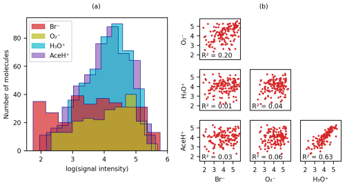
Figure 3 (a) Distribution of logarithmic signal intensities for molecules detected by each of the four ionization methods and (b) scatter matrix of logarithmic signal intensities for molecules detected by all reagent ions, illustrating correlations between different ionization signals.

Figure 3 presents the logarithmic signal intensity distribution (Fig. 3a) and the scatter matrix of the logarithmic signal intensity (Fig. 3b) for each reagent ion. In Fig. 3a, both AceH⁺ and H₃O⁺ are normally distributed. The distribution for ${\mathrm{O}}_{\mathrm{2}}^{-}$ is flatter (probably due to the small number of detected molecules), and Br⁻ is almost homogeneously distributed across the intensity range. Figure 3b visualizes the bivariate relationship between logarithmic signal intensities for the pesticides detected with all four reagent ions. Only the two positive polarity ionization schemes AceH⁺ and H₃O⁺ exhibit a clear correlation (R² = 0.6). The negative ionization schemes ${\mathrm{O}}_{\mathrm{2}}^{-}$ and Br⁻ are not as well correlated (R² = 0.2). Meanwhile, the inter-correlation between positive and negative reagent ions is below 0.07. The general lack of correlation between opposite polarity ionization schemes indicates that different reagent ions interact with the target molecules in distinct ways, possibly engaging with different functional groups.

Figure 4 shows the t-stochastic neighbor embedding (t-SNE; van der Maaten and Hinton, 2008) of the logarithmic signal intensity values for each compound. t-SNE visualizes high-dimensional data in lower dimensions preserving the local similarity of data points. We used the scikit-learn implementation of t-SNE (sklearn.manifold.TSNE; Pedregosa et al., 2011) with a random state of 42, a perplexity of 50 and a maximum number of iterations of 5000. We then assigned different colors and symbols to the ionization method combinations that detected a given pesticide.

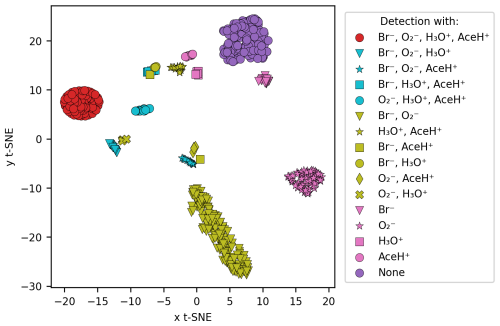
Figure 4 Similarity between the signal intensity of the molecules by using t-SNE clustering. The comparison was based on the logarithmic signal intensity, and each cluster follows a color code based on the detection type (all the possible combinations between the four reagent ions).

Clear clusters of the same color and the same symbol emerge in the t-SNE plot in Fig. 4. Only one cluster is composed of molecules detected with both Br⁻ and AceH⁺ (yellow squares); Br⁻ and H₃O⁺ (yellow circles); and Br⁻, AceH⁺ and H₃O⁺ (blue squares). From this we conclude that Br⁻ delivers the most information for these pesticides, and the positive polarity ionization method is of lesser importance. The situation is similar for H₃O⁺ and AceH⁺ that appear in two clusters where blue triangles (H₃O⁺, AceH⁺, Br⁻) come close to yellow crosses (H₃O⁺, ${\mathrm{O}}_{\mathrm{2}}^{-}$) and blue stars (AceH⁺, Br⁻, ${\mathrm{O}}_{\mathrm{2}}^{-}$) close to yellow diamonds (AceH⁺, Br⁻) and squares (AceH⁺, ${\mathrm{O}}_{\mathrm{2}}^{-}$). The presence of clear clusters suggests that, collectively, the reagent ions have the potential to differentiate between molecular structures.

3 Molecular descriptors

A molecular representation is a transformation of a molecular structure that simplifies the structural information into a readable input for data-driven methods. Depending on the application, they can provide a valuable cost-efficient alternative to computationally expensive quantum chemical computations. These descriptors are numerical representations of atomistic systems that should fulfill certain requirements, such as being invariant to spatial and rotational transformations, invariant to permutation of atomic indices, unique, continuous, compact, and computationally efficient (Himanen et al., 2020; Huo and Rupp, 2022; Rupp, 2015; Xue and Bajorath, 2000; Langer et al., 2022). Molecular descriptors may vary in complexity and interpretability; some reflect tangible properties that are easy for humans to understand, while others are calculated through mathematical means and may lack intuitive interpretation. However, a universal descriptor able to perform well for every chemical system and task does not exist. For this reason, being a first-of-a-kind study, we tested five different descriptors (Fig. 1a) for our classification task (prediction of the detection) and regression task (prediction of the CIMS signal intensity). We investigated a property-based descriptor (RDKitPROP), two structure-based descriptors (TopFP and MACCS) derived from SMILES (Simplified Molecular-Input Line-Entry System) strings, and two structure-based descriptors obtained from the Cartesian coordinates of the atoms in the molecules (CM and MBTR) (Landrum, 2006; Durant et al., 2002; Rupp et al., 2012; Huo and Rupp, 2022). The Cartesian coordinates were obtained from the SMILES string of each pesticide through geometry optimization with a universal force field implemented in RDKit (Landrum, 2006). Figure 5 depicts visual examples of four descriptors. The representations are discussed in more detail in the following sections.

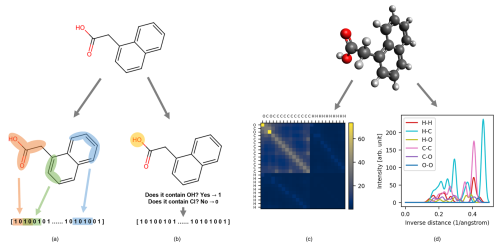
Figure 5 Visual example of 1-naphthaleneacetic acid molecular representations. On the left are descriptors computed from SMILES: (a) topological fingerprint (TopFP) and (b) molecular access system keys (MACCS). On the right are descriptors computed from Cartesian coordinates: (c) Coulomb matrix (CM) and (d) many-body tensor representation (MBTR).

3.1 Property-based descriptor (RDKitPROP)

RDKitPROP includes 43 properties computed from the molecular structure of the pesticides (represented by a SMILES string), by applying the function rdkit.Chem.rdMolDescriptors.Properties (Landrum, 2006). This descriptor was included in the analysis to evaluate the models' performance based on known properties that are computationally inexpensive to obtain. In the Supplement, we describe these properties in more detail (Table S4). In Sect. 5, we will discuss only a subset of the five most important properties for the best classifier (see Sect. 4.1). These properties are the topological polar surface area (TPSA; Ertl et al., 2000), the number of hydrogen bond donors (HBDs), the number of hydrogen bond acceptors (HBAs), the Wildman–Crippen logarithm of the partition coefficient (CrippenClogP; Wildman and Crippen, 1999), the fraction of sp³ carbons (FractionCSP3), the Hall–Kier alpha value (HallKierAlpha; Hall and Kier, 1991) and the molecular weight. TPSA calculates the polar surface area by summing the contribution of individual sub-structures containing nitrogen, oxygen, phosphorus and sulfur. The HallKierAlpha value is the sum of the scaled measures of each atom's covalent radius, adjusted for its hybridization state and electronegativity. The scaling is relative to the covalent radius of a sp³ hybridized carbon atom. CrippenClogP measures the hydrophobicity of a molecule, while FractionCSP3 indicates the saturation of carbon atoms in the molecule. The number of HBAs counts the oxygen and nitrogen atoms in the molecule. In the descriptor, two distinct properties address this value (LipinskiHBA and NumHBA). The number of HBDs calculates the number of hydrogen atoms attached to oxygen and nitrogen atoms in the molecule (addressed by LipinskiHBD and NumHBD). Lastly, the molecular weight is addressed as well by two distinct properties: the average molecular weight (AMw) and the exact molecular weight (ExactMw).

3.2 Topological fingerprint (TopFP)

TopFP (Fig. 5a) implemented in RDKit (Landrum, 2006) is a molecular descriptor inspired by the Daylight fingerprint (James et al., 1995). This fingerprint extracts molecular sub-structures of a certain size by starting from one atom and following the bond topology. A mathematical function converts each sub-structure into a bit string (hashing), and all strings are concatenated into the final fingerprint. In the implementation, the length of the sub-structure, the number of bits per hash and the final size of the fingerprint are called hyperparameters and can be optimized to improve the performance of the descriptor. TopFP is easily implemented at a reasonable computational cost. However, the hash function makes interpretation difficult as there is no one-to-one correspondence between sub-structures and bits.

3.3 Molecular access system keys (MACCS)

MACCS also encodes molecular features as binary string (Durant et al., 2002) (Fig. 5b). Unlike TopFP, however, bits correspond to the one-hot encoding of specific predefined questions, such as the following: “does the molecule contain a carbonyl group?” (yes: 1, no: 0). In this work we used the RDKit MACCS implementation, which encompasses a total of 166 keys (Landrum, 2006), making this descriptor fast to run. However, MACCS is limited in the number of implemented questions, and any structural or chemical information not captured by these questions is lost.

3.4 Coulomb matrix (CM)

The Coulomb matrix (M, Fig. 5c) encodes both the Cartesian coordinates and the nuclear charges of each atom in the molecule as a n×n matrix, where n is the number of atoms in the molecule:

$$\begin{array}{}\text{(1)}& {\mathbf{M}}_{IJ}=\left\{\begin{array}{ll}\mathrm{0.5}{Z}_I^{\mathrm{2.4}}& \forall I=J\\ {\displaystyle \frac{Z_I{Z}_J}{|R_I-R_J|}}& \forall I\ne J.\end{array}\right.\end{array}$$

Z_I is the atomic number of atom I and $|R_I-R_J|$ the Euclidean distance between the atoms I and J. The elements on the diagonal were fitted to atomic energies, while the off-diagonal elements encode a Coulomb repulsion between each atom pair in the molecule (Rupp et al., 2012). Compared to other three-dimensional representations, the CM is straightforward to interpret, easy to implement and fast to compute. This simplicity, however, comes with a loss of detail, e.g., bond connectivity, which may be relevant for representing larger molecules such as pesticides.

In this work, we used the DScribe (Himanen et al., 2020) implementation of the CM. The CM has no hyperparameters to optimize, which adds to its appeal.

3.5 Many-body tensor representation (MBTR)

The MBTR (f_K, Fig. 5d) captures the 3D structure of a molecule in a continuous way (Huo and Rupp, 2022):

$$\begin{array}{}\text{(2)}& f_K\left(x\right)={\displaystyle \frac{\mathrm{1}}{{\mathit{\sigma }}_K\sqrt{\mathrm{2}\mathit{\pi }}}}{e}^{-\frac{(x-g_K(K){)}^{\mathrm{2}}}{\mathrm{2}{\mathit{\sigma }}_K^{\mathrm{2}}}}.\end{array}$$

Here σ_K is the standard deviation of the Gaussian kernel, and g_K is a geometry function with input K for many-body rank k. The first term (k=1) encodes only elemental features (K=Z_i). The second term (k=2) records inverse or direct distances between atoms $K=\frac{\mathrm{1}}{|R_i-R_m|}$ or $K=|R_i-R_m|$ and the third term (k=3) angles between three atoms $K=\mathrm{\angle }(R_i-R_m,R_n-R_m)$ (or $K=\cos (R_i-R_m,R_n-R_m)$). Because the three terms are tabulated on a grid, this descriptor is the largest one we tested.

In this work, we used the DScribe (Himanen et al., 2020; Laakso et al., 2023) implementation of the MBTR. We used only the k=2 and k=3 terms, since including the first term did not improve the performance but increased the computation time (see Fig. S6 in the Supplement). We used inverse distances and the cosine for K=2 and K=3, respectively, and applied exponential weighting to determine the relative importance of each term. The tuned hyperparameters are the Gaussian broadening parameter σ₂ and σ₃ and the scale of the weighting referred to as w₂ and w₃ (Himanen et al., 2020).

4 Machine learning methods

In this section, we briefly introduce the two ML methods that we use in this work. Figure 2c presented a potential problem for the direct training of a regression model: for individual ionization methods, the data are imbalanced with a relatively high number of undetected pesticides. This imbalance suggests that there might not be enough instances to train a model able to generalize patterns and signals of the molecules, potentially leading to poor predictive performance. To tackle this problem, we decided to divide the CIMS signal prediction into a classification task and a regression task. To classify whether a pesticide is detectable or not with a specific ionization method, we will train a RF classifier. Subsequently, we will investigate whether we can predict the corresponding CIMS intensity with KRR.

4.1 Random forest classifier (RF)

RF (Breiman, 2001) is a ML method that combines different decision trees, each of which learns the relation between input and output features in terms of simple decision rules. Each tree is trained on a subset of the data and input features. Additional bootstrapping decreases the variance of the prediction by resampling the training set observations. In this work, we used a scikit-learn RF classifier (sklearn.ensemble.RandomForestClassifier). Each tree gives a class probability prediction (detected or undetected), and the final prediction is an average of the probability given by each tree. We optimized the following hyperparameters: the maximum number of estimators (the trees creating the forest) and the maximum depth of each tree (the length from the starting point, “root”, to the final points, “leaves”); the minimum number of samples per leaf, to ensure that each leaf has an adequate number of data points to avoid overfitting and underfitting; and the minimum number of sample splits, to ensure that each internal node (which can branch again) has an adequate number of samples.

4.2 Kernel ridge regression (KRR)

Regression is a statistical process that determines the strength and character of the relationship between one dependent variable and a series of other variables. In this work, we perform KRR to include non-linearities (kernel) and prevent over-fitting (ridge regression; Hoerl and Kennard, 1970).

The kernel model (f) is expressed as a linear sum over kernel functions k over the training samples x_i

$$\begin{array}{}\text{(3)}& f\left(\stackrel{\mathrm{̃}}{x}\right)=\sum _{i=\mathrm{1}}^n{\mathit{\alpha }}_{i}k\left(x_i,\stackrel{\mathrm{̃}}{x}\right).\end{array}$$

The expansion coefficients α_i follow from the minimization of the ridge loss function

$$\begin{array}{}\text{(4)}& \arg \underset{\mathit{\alpha }\in {\mathbb{R}}^n}{min}\sum _{i=\mathrm{1}}^n{\left(f\left(x_i\right)-y_i\right)}^{\mathrm{2}}+\mathit{\lambda }\Vert f{\Vert }_H^{\mathrm{2}}\to \mathit{\alpha }=(\mathbf{K}+\mathit{\lambda }\mathbf{I}{)}^{-\mathrm{1}}y.\end{array}$$

Here K is the kernel matrix, I is the identity matrix and $\Vert f{\Vert }_H$ is the norm of f in the feature space. We use the Gaussian kernel

$$\begin{array}{}\text{(5)}& k(x_i,x_j)=\exp \left(-{\displaystyle \frac{\Vert x_i-x_j{\Vert }_{\mathrm{2}}^{\mathrm{2}}}{\mathrm{2}{\mathit{\sigma }}^{\mathrm{2}}}}\right),\end{array}$$

where σ is the length-scale hyperparameter. In this work, we applied the KRR implementation (sklearn.kernel_ridge.KernelRidge) from scikit-learn.

4.3 Performance metrics

Different performance metrics will be adopted to evaluate the performance of the classifier and the regressor methods. For the classification task, the performance will be evaluated using two metrics: accuracy and the receiver operating characteristic (ROC) curve. The accuracy score is the fraction of correct predictions compared to the total number of observations present in a test set:

$$\begin{array}{}\text{(6)}& \mathrm{accuracy}(y,\widehat{y})={\displaystyle \frac{\mathrm{1}}{n}}\sum _{i=\mathrm{0}}^{n-\mathrm{1}}\mathrm{1}({\widehat{y}}_i=y_i),\end{array}$$

where ${\widehat{y}}_i$ is the ith predicted class, y_i is its reference class and n is the number of samples in the test set.

In the case of the RF classifier, the model outputs probability scores for each class, and then a threshold is applied to determine the final class label, the predicted class. The ROC curve provides us with an additional performance assessment. The curve puts the correctly classified pesticides (true positive rate, vertical axis) in relation to the incorrectly classified ones (false positive rate, horizontal axis), across a range of different threshold levels. By varying the threshold used to convert probability scores into class labels, we can observe the model's performance across different operating points. The area under the curve (AUC) quantifies the overall ability of the classifier to distinguish between the two given classes (Géron, 2022). The more the curve shifts towards the top-left corner (with an AUC corresponding to 1), the better the classification. A random classifier would correspond to a diagonal line with an AUC of 0.5.

The regression performance will be assessed with the mean absolute error (MAE), a metric commonly used to measure the average absolute difference between a variable's predicted and reference values. Unlike other metrics, MAE does not penalize outliers as it assigns equal weight to all errors (Rupp, 2015). The MAE is defined as

$$\begin{array}{}\text{(7)}& \mathrm{MAE}(y,\widehat{y})={\displaystyle \frac{\mathrm{1}}{n}}\sum _{i=\mathrm{0}}^{n-\mathrm{1}}\left|y_i-{\widehat{y}}_i\right|,\end{array}$$

where ${\widehat{y}}_i$ is the predicted value of the ith sample, y_i is the corresponding true value in the dataset and n is the number of observations.

4.4 Computational details

We train a separate classification and regression model for each ionization method. The datasets were randomly split into test (20 %) and training (80 %) sets, ensuring that the trained model's performance is evaluated with an out-of-sample subset of data. The training set is further split into six subsets to create a learning curve. Each model was trained with five different random splits (i.e., different random seeds) to average out data variability and to collect statistics. Additionally, we optimized the hyperparameters with 5-fold cross-validation using random search implemented by scikit-learn (sklearn.model_selection.RandomizedSearchCV), which is efficient in higher dimensions (Stuke et al., 2021).

We trained binary classifiers that distinguish only between two classes (class 1: detected, class 0: undetected), for which we have a maximum of 554 training points (80 % of the data). The regressors were trained on the logarithmic CIMS intensity of the detected pesticides. Before training, we log-transformed the non-zero CIMS intensities to create a normal-like distribution, reducing outliers' impact and stabilizing variance. MAE is then reported on this log scale, showing the model's error in terms of order-of-magnitude accuracy. This gives us a maximum of 240 training data points for Br⁻, 174 for ${\mathrm{O}}_{\mathrm{2}}^{-}$, 376 for H₃O⁺ and 379 for AceH⁺.

In Sect. S4 of the Supplement, we provide the optimized hyperparameters for each model and each random seed. Tables S6, S7, S8, S9 and S10 report the RF hyperparameters and Tables S11, S12, S13, S14 and S15 the KRR hyperparameters for each molecular descriptor.

5 Results and discussion

In this section, we present and evaluate the performance of our trained models. For the classification, we examine the ability of our RF models to predict the detected or undetected compounds in the test set. For the regression, we investigate whether our KRR models can accurately predict the CIMS sensitivity of the test set compounds. Furthermore, we analyze which descriptors most effectively enhance model performance and explore whether chemical qualitative insights can be derived from them.

5.1 CIMS detection prediction

The classification ROC curves and relative AUC values for each ionization scheme are presented in Fig. 6 for the five molecular descriptors. All ROC curves lie above the diagonal, which implies that our RF models can classify if a pesticide is detectable based on its atomic and chemical structure. However, they do so with varying degrees of success. The best performance is achieved with the MACCS, MBTR and RDKitPROP descriptors, with average AUC values above 0.86. The TopFP and CM descriptors perform worse, in particular for the negative ionization schemes, most likely due to the smaller number of training samples.

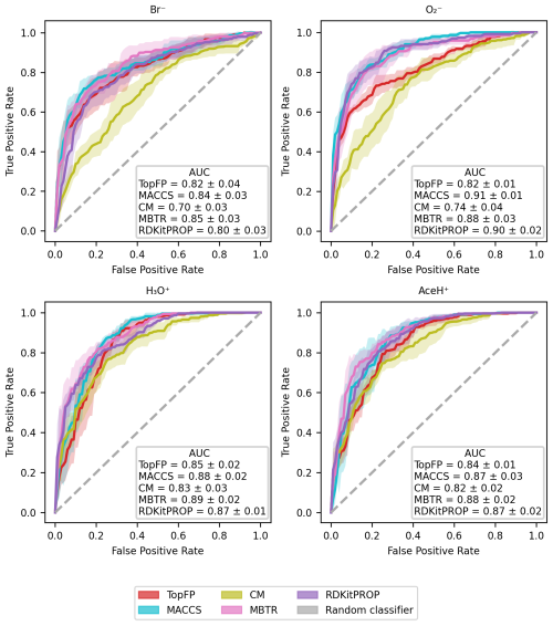
Figure 6 Evaluation of the classification performance with RF, by the use of ROC curves for the four ionization schemes (Br⁻, ${\mathrm{O}}_{\mathrm{2}}^{-}$, H₃O⁺, AceH⁺) with the five molecular descriptors (MACCS, MBTR, TopFP, CM, properties). For each curve, we report the AUC value. The x axis reports the false positive rate, and the y axis reports the true positive rate. The mean value and standard deviation are obtained by repeating the training with five different random re-shuffles of the dataset.

Table 2 reports the classification accuracy for each reagent ion over five random re-shuffles of the datasets. The learning curves for the accuracy can be found in the Supplement (Fig. S7), where we also present the learning curves for similar performance metrics such as recall, precision and F1 score (Figs. S8, S9 and S10, respectively). All classification models reach an accuracy above 0.6. The CM descriptor shows the worst overall performance for Br⁻ (0.64 ± 0.04 of accuracy), and MACCS reaches the best overall performance for H₃O⁺ (0.85 ± 0.02 of accuracy). In general, the accuracy is worse for Br⁻, while ${\mathrm{O}}_{\mathrm{2}}^{-}$ is on par with H₃O⁺ and AceH⁺. Overall, MBTR and MACCS yield the highest accuracy, followed by TopFP and RDKitPROP and then CM.

Table 2 Accuracy mean value and standard deviation of the prediction on the test dataset with RF for all reagent ions with the five different molecular descriptors. The values were obtained by repeating the training on the largest training size (80 % of the dataset), with five different random re-shuffles of the dataset.

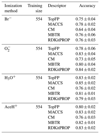
MBTR is the largest and most complex descriptor we have tested. Its good performance is similar to previous observations for vapor pressure (Lumiaro et al., 2021) and ionization energy predictions (Stuke et al., 2019). The fact that the MACCS key achieves a similar performance is at first surprising because it performed poorly in the earlier studies. The good classification performance reported here, however, indicates that the chemical complexity of the pesticides is well captured by the questions encoded in the MACCS keys.

The ROC curves and the accuracy metrics demonstrate good discriminative capabilities for predicting pesticide detection. This performance is particularly noteworthy given the challenges posed by the class imbalance in the dataset and the relatively small training set of just 554 observations, which is modest compared to typical ML applications. The fact that all models classify well indicates that they can capture the inherent chemical and structural diversity of the pesticides, which can provide additional insight into the interaction between the target molecules and reagent ions (see Sect. 5.3).

With an accuracy and AUC of around 0.8 our best-performing models are good enough to be useful in deployments. We expect that the trained models can predict detection with CIMS (specifically with Br⁻, ${\mathrm{O}}_{\mathrm{2}}^{-}$, H₃O⁺, or AceH⁺ as reagent ions) for molecules with similar structural features to those in our dataset. This could speed up laboratory analyses or field deployment for measuring campaigns or safety and security systems since one can a priori check if a pesticide will be detectable without having to perform a CIMS experiment.

5.2 Quantitative prediction of CIMS sensitivity to target molecules

We now turn to evaluate the performance of the regression models tasked to predict the CIMS sensitivity of the pesticides. The MAE learning curves of the KRR models are shown in Fig. 7 for five random seeds and the different descriptors. For all the reagent ions, the MAE decreases with increasing training size indicating that our models indeed learn with data. The learning rate is comparable to earlier work (Lumiaro et al., 2021; Stuke et al., 2019) that used much larger datasets. Usually, the variance decreases with increasing dataset size, which is not the case in Fig. 7. We attribute the variability in learning curves to the small size of the training dataset. When subsets of data are selected using different random seeds, the limited number of observations leads to inconsistent sampling of data patterns, which prevents the model from stabilizing, particularly against outliers. As a result, the variance across learning curves as the training set size grows remains high due to the small sample size.

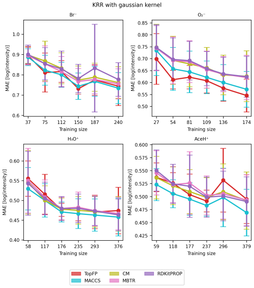
Figure 7 Learning curve with mean absolute error (MAE) of the signal intensity values in logarithmic scale of Br⁻, ${\mathrm{O}}_{\mathrm{2}}^{-}$, H₃O⁺ and AceH⁺ datasets, based on the TopFP, MACCS, CM, MBTR and properties as the descriptors. The x axis reports the training set size, and the y axis reports the MAE of the logarithmic signal intensity. The mean value and standard deviation are obtained by repeating the training with five different random re-shuffles of the dataset.

Table 3 presents the average MAE values for the highest training size for each ionization method and descriptor averaged over the five random seeds. All trained models achieved an error lower than one logarithmic unit of signal intensity. Such low MAEs present a significant achievement considering both the complex task and the small size of the dataset and the fact that CIMS signals vary over several orders of magnitude.

Table 3 Mean absolute errors (MAEs) and standard deviation of the prediction on the test dataset with KRR for all reagent ions with the five different molecular descriptors. The values were obtained by repeating the training on the largest training size (80 % of the detected dataset) with five different random re-shuffles of the dataset.

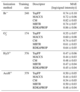
We find the lowest MAEs for the positive polarity ionization methods, most likely because the available datasets are larger. Unlike classification, the different descriptors perform similarly to the regression task. Overall, MACCS is still the best, followed by TopFP and MBTR. The fact all descriptors learn similarly is surprising since they capture different features of the elemental and structural features. We believe this behavior stems from the inherent characteristics of the dataset. The noise and variability in the data could obscure the potential advantages of these more complex descriptors. Moreover, since we employed KRR as our regression model, its ability to learn intricate patterns might be limited by the inherent challenges present in the data.

The results demonstrate that all models can achieve a MAE under one unit of logarithmic signal intensity, which is impressive, especially considering the even lower number of observations compared to the classification task (174 in the worst case). Such an accuracy is already sufficient for deployment in field studies. For suspected molecules or pollutants, ML models could estimate the expected signal intensity and subsequently its concentration in the atmosphere without relying on quantum chemical computations or direct measurements. Conversely, insight into the detection processes could be garnered by identifying chemical features that correlate with the signal intensity for the different ionization methods. We will present such analysis in the next section.

5.3 Chemical insight

Next, we explore the chemical insight our ML classification models offer into ion–molecule interactions. As a proof of concept, we aim to relate the model's findings to established knowledge and note any unexpected influential features. We focus on the RF classifier model, as it enables straightforward identification of key molecular features associated with signal detectability. This is achieved by analyzing which features are most influential in the RF model's classification decisions. We will focus on the MACCS and RDKitPROP descriptors because they are the most interpretable. In the case of MACCS, the insight into the interaction can be extracted by analyzing the occurrence of molecules detected and not detected for each feature, i.e., each MACCS key (sub-structure) of the molecular structure. In the case of RDKitPROP, the insight into the interaction can be formulated by analyzing each feature, i.e., property. For each ionization method, we pick the largest training set size and then obtain the feature ranking and the corresponding coefficients (importance values) from the trained RF models for the five random seeds. We then average the importance values for each feature and rank again. For each ionization method, we pick the largest training set size and then obtain the feature ranking and the corresponding coefficients (importance values) from the trained RF models for the five random seeds. We then average the importance values for each feature and rank again.

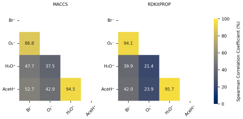
Figure 8 Pearson correlation coefficient (%) of the normalized features importance values obtained from the RF estimator trained on 80 % of the data with optimized hyperparameters based on MACCS and RDKitPROP.

We then compare the most important features of a given ionization method to those of the other ionization methods by means of the Pearson correlation coefficient. Figure 8 shows the Pearson correlation coefficient of the normalized feature importance values in percentage for the RDKitPROP and MACCS descriptors. For both descriptors, the features for the negative (Br⁻ and ${\mathrm{O}}_{\mathrm{2}}^{-}$) and positive polarity ionization methods (H₃O⁺ and AceH⁺) correlate strongly (above 86.8 %). The inter-correlation between the features of the positive and negative reagent ions, however, is much weaker (between 21.4 % and 52.7 %). The Pearson correlation coefficients reveal that the polarity of the reagent ion predominately determines which molecular features the ion interacts with. We made a similar observation in Fig. 3b, where we saw that the signal intensities cluster strongly by the polarity of the reagent ion.

Figure 9 reports the importance values in percentage for the most important features of the RDKitPROP model for the four ionization methods. Tables S16 and S17 in the Supplement provide the values for all the properties, and additionally, the average value of the property is calculated individually for detected and undetected pesticides. No feature has an importance above 10 %, and only four of them reach an importance above 6 %: TPSA and LipinskiHBA in the case of positive reagent ions and LipinskiHBD and NumHBD in the case of negative reagent ions. The next most important properties are NumHBA and NumAtoms for positive polarity ionization methods and then HallKierAlpha, CrippenClogP, FractionCSP3, AMw and ExactMw presenting similar importance for both positive and negative polarity ionization methods.

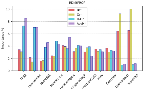
Figure 9 RDKitPROP RF best estimator features importance (%) of a subset of properties for each ionization method.

As mentioned in Sect. 3.1, some properties present repetitive information, which means that the overall importance relative to the number of HBDs, as an example, is shared between the NumHBD property and the LipinskiHBD property. Either property probably would have reached a higher importance if only one of the two had been considered. The other two properties that present repetitive information are the number of HBAs (with importance shared between NumHBA and LipinskiHBA) and the molecular weight (with importance shared between AMw and ExactMw). Going into more detail, the number of HBDs correlates strongly with negative polarity ionization methods and the number of HBAs with positive ones. This behavior is expected because the HBD quantifies the number of hydrogen atoms attached to either oxygen or nitrogen atoms. Both of these groups can create a hydrogen bond and thus promote the interaction with negative reagent ions. Conversely, the HBA encodes the number of oxygen or nitrogen atoms in the molecule, which can both create a hydrogen bond and accept a proton, promoting the interaction with positive reagent ions.

The high importance of TPSA highlights the significance of the molecular polar surface in the ionization mechanism. The polarity of the target molecule can increase the chances of interacting with the reagent ion, therefore increasing the resulting signal intensity. The tendency of ionization, and thus the CIMS signal intensity, then increases with increasing polarity. Notably, our models assign a higher importance to the polarity for positive reagent ions, possibly due to the higher number of detected pesticides in the data. However, it is important to note that TPSA was originally calculated and implemented by not including halogen contributions in the equation (Ertl et al., 2000; Landrum, 2006). Therefore, the high presence of bromine, fluorine and iodine atoms in pesticides influences the polarity and might result in a different polar surface area.

Similar to TPSA, CrippenClogP emphasizes the role of hydrophilicity in our interaction analysis. The importance of molecular weight and NumAtoms indicates that larger molecular size correlates with detectability, as it provides more functional groups and a greater collision cross-section, thereby possibly increasing the likelihood of interactions with the reagent ion.

HallKierAlpha was also found useful in predicting molecular detection characteristics, which indicates that for each molecule the sum of the scaled measures of each atom's covalent radius (adjusted for its hybridization state relative to the covalent radius of a sp³ hybridized carbon atom) relates to the reagent ion–target molecule interaction. For all ionization methods, both detected and undetected molecules have negative HallKierAlpha values (see Tables S16 and S17), suggesting that the molecules in the dataset generally have smaller average atomic sizes relative to a sp³ hybridized carbon atom. Detected molecules exhibit, on average, a smaller HallKierAlpha value than undetected ones. However, it is not clear if this difference in HallKierAlpha values is statistically significant.

The presence of FractionCSP3 among the most important features indicates that the fraction of sp³ hybridized carbons in the molecule contributes to the reagent ion–molecule interaction. With an in-depth analysis, the data suggest that molecules with a “rigid” structure (fewer sp³ carbons) slightly prefer interaction with negative reagent ions, while molecules with flexible structures (more sp³ carbons) slightly prefer interaction with positive reagent ions.

We observe that several of the identified important features relate to proton affinity. The number of HBAs (NumHBA, LipinskiHBA) is directly correlated to proton affinity as it calculates the number of sites available to accept a proton. The TPSA describes the molecule's polarity, and for certain molecules, a higher TPSA could correlate with a higher proton affinity. HallKierAlpha correlates as well since every atom's covalent radius is adjusted for its hybridization state and electronegativity, reflecting the likelihood of atoms within a molecule to donate electron density to a proton. FractionCSP3, while not correlating directly to proton affinity, might influence the overall basicity of the molecule (e.g., a higher number of sp³ carbons in the molecule potentially affects the electron density of heteroatoms indirectly).

We note that different reagent ions react with the analyte in distinct ways (see the Introduction). While our results support the predictive nature of properties like proton affinity, specifically for positive reagent ions, the ML model's advantage lies in its flexibility. As shown, this approach aligns well with established knowledge, yet the ML methodology combined with molecular representations can relate any reagent ion or ionization mechanism to the magnitude of CIMS signals using only the analyte molecular structure.

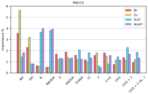
Figure 10 MACCS RF best estimator features importance (%) of a subset of MACCS keys for each ionization method.

Figure 10 reports the importance values in percentage of a representative subset of the 50 most important keys (e.g., reaching 1 % importance for at least one ionization method) of the MACCS descriptor for the four ionization methods (the remaining important keys can be found in Tables S18 and S19 in the Supplement). We find no key with importance above 6 %, suggesting that in complex systems such as pesticides, no single structural or chemical feature dominates the interaction with the reagent ions. Instead, multiple features of the molecule participate in the interaction, by connecting either actively to the reagent ion or passively through, e.g., inductive effects that increase the bond strength. It is also important to remember that our dataset is quite diverse. Thus, specific features or functional groups could have different importance for different types of molecules, decreasing the overall importance values. The groups with the highest importance are amines (NH, either primary or secondary) and hydroxyl (OH) for negative reagent ions and nitrogen and nitrogen atoms with three single bonds (NA(A)A, where “A” stands for any element) for positive reagent ions. All other features do not surpass 2.5 % of importance, on average.

Table 4 MACCS-based RF best estimator feature importance (%) of a subset of structural keys (groups). For each key, the structure, the importance value (IMP, %) and the proportion of presence (PP, %), with, in addition, the average group count per molecule (Avg) for detected (D) and undetected (ND) molecules, are stated. In the name of the structures, the special characters stand for “A”, any element; “X”, halogen; “!”, chain or non-ring bond; and “$”, ring bond.

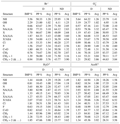
Additionally, Table 4 reports a subset of the 50 most important MACCS features. The table reports individually for each reagent ion: the key (sub-structure), its importance value (IMP, %), the proportion of appearance in the dataset (PP %) and the average count of the appearing key per molecule (Avg) (calculated individually for detected (D) and undetected (ND) pesticides).

NH is most important for Br⁻ and ${\mathrm{O}}_{\mathrm{2}}^{-}$ (3.56 % and 5.64 % of importance respectively). It is nearly twice as important for detected than undetected pesticides (approx. 57 % vs. approx. 24 %). With 2.29 % and 3.19 %, the importance of OH is slightly lower than for NH. Like NH, OH groups trigger predominately for detected pesticides (approx. 23 % for detected vs. 6 % for undetected molecules). For both OH and NH groups, the undetected pesticides had a higher average frequency of appearance (Avg, how many times a group is present in a molecule, for the full dataset on average, by considering only the detected or undetected cases). However, we note that negative reagent ions suffer from a class imbalance, and the high number of undetected cases could influence this statistic.

Both OH and NH are HBD groups. OH is known to be important for the interaction with negative reagent ions, while the importance of NH groups for this interaction has been observed by quantum chemical calculations in Partovi et al. (2023). With our ML models, we find these relations solely through patterns in the data.

For positive ionization schemes, OH groups do not reach 1 % of importance and do not present any relevant variation between detected and undetected. Amine groups reach 1 % of importance and correlate with detected pesticides (44 % for detected vs. 19 % for undetected molecules). For AceH⁺ ionization, NH is only the 4th most important feature. The most important groups for positive ionization are instead those containing nitrogen. Being a HBA, nitrogen is an element that can facilitate the interaction between reagent ions and sample molecules.

The presence of nitrogen (N in the table) reaches 3.65 % and 4.00 % in importance for H₃O⁺ and AceH⁺. In both datasets, N appears approximately in 88 % of the detected pesticides and in 52 % of the undetected pesticides. Similarly, NA(A)A groups reach 3.80 % and 3.93 % of importance for H₃O⁺ and AceH⁺. This group is common in the studied dataset (for positive reagent ions: approximately 83 % for detected but only 42 % for undetected pesticides).

Next, we will analyze other groups with importance for both positive and negative reagent ions. Five important features relate to the presence of halogens: the first three indicate if a halogen is present (X), if it has three single bonds (XA(A)A) and if it is bonded to a ring (X!A$A, where “!” stands for a chain or non-ring bond and “$” stands for a ring bond). The last two specify whether the halogen is a chlorine (Cl) or fluorine (F) atom. These halogen-related features range between 1 % and 2 % in importance across the four ionization schemes (F is the only one not reaching 1 % of importance for positive reagent ions). For negative reagent ions, these groups are 10 %–20 % more prevalent in detected than undetected pesticides. However, the average frequency of appearance per molecule between detected and undetected molecules does not present any clear difference. In contrast, molecules detected by positive reagent ions have 15 %–20 % fewer halogen features than undetected molecules (specifically for the groups X, XA(A)A, X!A$A). The frequency of appearance per molecule is also higher for undetected pesticides, with an average of three to six groups per molecule (compared to two to three groups per molecule for detected instances). F shows the opposite trend for positive reagent ions. It has a slightly higher presence and a higher average group frequency for detected molecules. However, as previously stated, F does not reach 1 % of importance for positive ionization schemes, so this result might not be as relevant as for the other features. In summary, the presence of halogens in a molecule enhances the detectability of negative ionization schemes and reduces it for positive ones.

The carbonyl group has a moderate importance (< 2 %) for all ionization schemes. For Br⁻ and ${\mathrm{O}}_{\mathrm{2}}^{-}$, the importance is 1.8 % and 1.52 % and for H₃O⁺ and AceH⁺ 0.82 % and 1.57 %, respectively. Focusing on negative reagent ions, C=O appears approximately in 70 % of the detected pesticides and in 50 % of the undetected ones, with a similar frequency per molecule (1.3 times). Carbonyl is a HBA group. Its importance for negative ionization schemes could therefore be due to either an inductive effect of oxygen or a possible redirection of the reagent ion to HBD groups. For positive reagent ions, C=O is present in approximately 64 % detected and 40 % undetected molecules, following its ability to accept hydrogens.

Among the important MACCS keys, we find three which enumerate whether there is one, more than one or more than two methyl groups (CH₃, CH₃ > 1 and CH₃ > 2). The positive ionization schemes show a greater prevalence of these features for detected pesticides than the negative schemes. For positive reagent ions, CH₃ is most important when it appears two times in a molecule.

Overall, RDKitPROP and MACCS in combination with RF have given us valuable insights into CIMS ion–molecule interactions. In the case of positive polarity ionization methods, the results obtained with the chemical insight analysis support known alternative methods of identifying whether a molecule can be detected, by highlighting a series of properties that can relate to proton affinity. In the case of negative polarity ionization methods, a substantial comparison can be made with literature findings, mainly based on detailed quantum chemical calculations. Based on RDKitPROP, the number of HBDs in the molecule was attributed more than 10 % of importance (by combining LipinskiHBD and NumHBD percentages), while based on MACCS, HBD groups such as OH and NH were found among the most important ones.

These results agree with atmospheric chemistry studies such as Iyer et al. (2016) and Hyttinen et al. (2018), where quantum chemical calculations indicated that for organic vapors, OH is the primary functional group interacting with negative reagent ions. Similarly, Partovi et al. (2023), in a study of pesticide molecules, identified NH groups as significant in interactions with Br⁻ when OH groups were absent. Thus, our model supports these findings by identifying important features directly from data patterns without needing intensive quantum chemical methods.

While previous studies focused on single compound classes (e.g., homogenous sets of volatile organic compounds), or in a limited amount of complex compounds, our method utilizes a less homogeneous and larger dataset. The chemical insight analysis of our work provides a general profile of the interaction mechanism, supporting the findings from the literature but also highlighting other functionalities that might affect the signal due to their relation to the electronic structure.

This data-driven approach also required minimal computational resources due to the simplicity of the RDKitPROP and MACCS descriptors, contrasting with the higher demands of quantum chemical calculations. Although quantum chemical approaches remain essential for detailed, molecule-specific interactions, our ML model effectively reveals broader trends, distinguishing between detected and undetected molecules across the four studied ionization schemes.

6 Conclusions

In summary, we developed a ML workflow for predicting the detection with CIMS (with a classification algorithm) and CIMS sensitivity to molecules (with a regression algorithm) to improve atmospheric compound identification. The goal is to evaluate if our ML model can accurately predict detections and signal intensities, thus offering a foundation to build a database of simulated compounds' signals for compound identification purposes with CIMS. Currently, compound identification is typically achieved by comparing an unknown compound's spectrum to a reference database. While this work does not provide direct identification of unknown compounds, it establishes a methodology for developing such a database, which could be expanded for broader use in atmospheric chemistry.

Two standard solutions containing 693 pesticides were analyzed with the Orbitrap TD-MION-MS. A RF classifier and a KRR model were trained on five different molecular structure representations. The best descriptor found is MACCS for both the classification and the regression. In the case of classification, MACCS reaches 0.85 ± 0.02 of accuracy and AUC of 0.91 ± 0.01; in the case of regression, MACCS can reach 0.44 ± 0.03 of MAE in logarithmic units of signal intensity. Models based on this descriptor have the lowest errors in both algorithms and are also easy to understand and implement, as they encode the presence of functional groups, or sub-structures starting from SMILES strings. Because of its white-box nature, the MACCS descriptor can provide chemical insight. Our feature importance analysis of the RF classifier provided insight into the reagent-ion interaction. RDKitPROP highlighted trends in the data that are generally known from basic chemical intuition. The feature analysis of the MACCS-based model highlighted the possible sub-structures that might impact the detection of the molecules. Models based on the two negative polarity ionization methods, Br⁻ and ${\mathrm{O}}_{\mathrm{2}}^{-}$, presented similar results, such as the high importance of OH and NH groups, and carbonyls and halogens. Positive polarity ionization methods, H₃O⁺ and AceH⁺, also presented similar results and highlighted the key role of nitrogen in detection and halogens in decreasing the chances of detection. These are the most relevant features found for the ML model, which generalizes features of experimental data.

The results demonstrate that it is possible to extract predictive information even in small experimental datasets. However, more instances could help to generalize the structural features better and help prevent class imbalance problems. Currently, our ML models are directly applicable to predicting the detection and signal intensity of molecules with molecular structures similar to those in our dataset. For molecules with more diverse structures, transfer learning approaches could use these trained models as a baseline, updating learned parameters to accommodate the characteristics of new structures.

Applying our approach directly to field measurements will require a comprehensive, standardized dataset of atmospheric compounds with a limited number of reagent ions for practical applications. Such a dataset could facilitate accurate mapping of ionization tendencies, potentially enabling compound identification directly from field CIMS measurements in the future. Moreover, while this workflow was developed using high-resolution Orbitrap data, it can also be utilized with lower-resolution data, though this may introduce greater uncertainties.

The ML models developed in this work are a first step towards optimizing CIMS measurements for comprehensive reaction product detection with ML, aiming to enhance the general understanding of complex analyses such as those of atmospheric CIMS in the future. In future work, studying datasets with similar structures to atmospheric compounds (focusing on oxygenated compounds) could bring a greater understanding of the reagent ion and sample molecule interaction inside the instrumentation, thereby providing a greater understanding of the compounds detected in situ atmospheric measurement. An improvement in the ML performance could come from both experimental data and synthetic data. Furthermore, the development of standardized experimental datasets is crucial, as these can significantly boost the possibility of using artificial intelligence algorithms and enhance the accuracy and reliability of future atmospheric analyses.