the Creative Commons Attribution 4.0 License.
the Creative Commons Attribution 4.0 License.
 | 27 Jun 2025
Data-driven modeling of environmental factors influencing Arctic methanesulfonic acid aerosol concentrations
William H. Aeberhard
Michele Volpi
Eliza Harris
Benjamin Hohermuth
Sakiko Ishino
Ragnhild B. Skeie
Stephan Henne
Patricia K. Quinn
Lucia M. Upchurch
Natural aerosol components such as particulate methanesulfonic acid (MSAp) play an important role in the Arctic climate. However, numerical models struggle to reproduce MSAp concentrations and seasonality. Here we present an alternative data-driven methodology for modeling MSAp at four High Arctic stations (Alert, Gruvebadet, Pituffik (formerly Thule), and Utqiaġvik (formerly Barrow)). In our approach, we create input features that consider the ambient conditions experienced during atmospheric transport (e.g., dimethyl sulfide (DMS) emission, temperature, radiation, cloud cover, precipitation) for use in two data-driven models: a random forest (RF) regressor and an additive model (AM). The most important features were selected through automatic selection procedures, and their relationships with MSAp model output was investigated. Although the overall performance of our data-driven models on test data is modest (max. R2=0.29), the models can capture variability in the data well (max. Pearson correlation coefficient = 0.77), outperform the current numerical models and reanalysis products, and produce physically interpretable results.
The data-driven models selected features which can be grouped into three categories, the sources, chemical processing, and removal of MSAp, with specific differences between stations. The seasonal cycles and selected features suggest gas-phase oxidation is relatively more important during peak concentration months at Alert, Gruvebadet, and Pituffik (Thule), while aqueous-phase oxidation is relatively more important at Utqiaġvik (Barrow). Alert and Pituffik (Thule) appear to be more influenced by processes aloft than in the boundary layer. Our models usually selected chemical-processing-related features as the main factors influencing MSAp predictions, highlighting the importance of properly simulating oxidation-related processes in numerical models.
- Article
(7863 KB) - Full-text XML
-
Supplement
(3282 KB) - BibTeX
- EndNote


Natural marine biogenic aerosols, e.g., particulate methanesulfonic acid (MSAp), are becoming an increasingly important part of the Arctic climate system, especially during summer, due to sea ice retreat as well as changing environmental conditions and circulation patterns (Willis et al., 2023), yet their environmental drivers remain understudied (Schmale et al., 2021). Processes leading to natural aerosol emissions are affected by climate change, leading to ongoing changes in the natural aerosol baseline. Understanding natural aerosols has implications for accurate modeling of the pre-industrial atmosphere and thus estimation of the indirect aerosol effect (Carslaw et al., 2013; Menon et al., 2002). Natural aerosols, such as MSAp, are important seeds for low-level mixed-phase clouds in the Arctic (Abbatt et al., 2019; Beck et al., 2021). Low-level clouds can have a significant effect on the surface energy budget, influencing snow cover, sea ice extent, and the Greenland ice sheet behavior (Arouf et al., 2024; Wendisch et al., 2019). The current understanding of the Arctic climate system is limited, due to, amongst other reasons, an insufficient representation of low-level Arctic mixed-phase clouds in large-scale models (Morrison et al., 2012; Pithan et al., 2016; Taylor et al., 2022). The inadequate representation of aerosol particles acting as cloud condensation nuclei and ice-nucleating particles may partly explain the shortcomings of cloud representation in large-scale models (Mauritsen et al., 2011; Stevens et al., 2018). While significant progress has been made (Abbatt et al., 2019; Shupe et al., 2022; Wendisch et al., 2019, 2024), there are still important gaps in the current understanding and modeling efforts of natural Arctic aerosols (Schmale et al., 2021).
In the Arctic atmosphere, MSAp mainly derives from the oxidation of natural, marine emissions of dimethyl sulfide (DMS) (Barnes et al., 2006a), although other sources can make minor contributions such as lakes, coastal tundra, melt ponds, and biomass burning (Levasseur, 2013; Mungall et al., 2016; Park et al., 2019). Arctic marine phytoplankton and algae produce dimethylsulfoniopropionate as an osmoprotectant (Yoch, 2002), which is enzymatically cleaved to produce seawater DMS (Andreae, 1990; Kettle et al., 1999), which is the main source of marine biogenic sulfur in the atmosphere (Hulswar et al., 2022; Lana et al., 2011). Although the majority of DMS is oxidized within seawater, a fraction is ventilated into the atmosphere where it is photochemically oxidized by OH, O3, NO3, and halogen species via two pathways (addition or abstraction), both of which depend on temperature (Barnes et al., 2006a; Jiang et al., 2021; Shen et al., 2022). The atmospheric lifetime of DMS is on the order of 1–2 d (Breider et al., 2010; Lundén et al., 2007), depending on latitude and environmental conditions (Ghahreman et al., 2019). DMS oxidation to MSAp involves a variety of gas- and aqueous-phase reactions, the latter occurring in cloud droplets or on deliquesced particles (Barnes et al., 2006a; Chen et al., 2018; Fung et al., 2022; Hoffmann et al., 2016). DMS is first oxidized through two major branches. One is the abstraction pathway by reactions with OH, NO3, and Cl radicals in the gas phase to yield methylthiomethylperoxy radical (MTMP: CH3SCH2OO) (Berndt et al., 2019; Hoffmann et al., 2016). MTMP can undergo isomerization to form hydroperoxymethylthioformate (HPMTF) (Berndt et al., 2019; Veres et al., 2020) or oxidation by NO or RO2 to produce CH3SO2, which can then form SO2, sulfuric acid (H2SO4), or MSA with strongly temperature-dependent yields (Berndt et al., 2023; Chen et al., 2023; Shen et al., 2022). The other DMS oxidation branch is the addition pathway through reactions with OH, BrO, Cl, and O3 to yield dimethyl sulfoxide (DMSO), which occurs mainly through the gas phase but partly in the aqueous phase through reaction with O3 (Hoffmann et al., 2016). DMSO is a semi-volatile species which reacts with OH in both the gas and aqueous phase to form methanesulfinic acid (MSIA). MSIA then reacts with OH or O3 in the aqueous phase to produce MSAp (Chen et al., 2018; von Glasow and Crutzen, 2004; Hoffmann et al., 2016; Wollesen de Jonge et al., 2021), although it can also undergo gas-phase oxidation by OH to yield CH3SO2, thus contributing to the temperature-dependent pathway to produce gaseous MSA (Chen et al., 2023; Shen et al., 2022). The produced gas-phase MSA can condense onto cloud droplets or existing particles to form MSAp (Hoffmann et al., 2016). Aqueous-phase reactions are dominant formation mechanisms for MSAp in a typical marine boundary layer condition (Baccarini et al., 2021; Chen et al., 2018; Hoffmann et al., 2016; Kecorius et al., 2023). In the Arctic, cold temperatures (Barnes et al., 2006a; Chen et al., 2023; Shen et al., 2022) and elevated halogen levels will favor MSA/MSAp formation relative to SO2 (Chalif et al., 2024; Jongebloed et al., 2023; Sørensen et al., 1996) especially in the springtime, through both gas- and aqueous-phase pathways. The presence of ice-containing clouds may limit the aqueous-phase production since reactions between DMS and its intermediates and oxidants are mainly able to occur at the surface (Chen et al., 2018). For a full description of DMS oxidation mechanisms and pathways, see Barnes et al. (2006a). After formation in the aqueous phase, MSAp can be released into the gas phase during droplet evaporation and go on to further impact secondary aerosol production (Baccarini et al., 2021; Fung et al., 2022; Kecorius et al., 2023). Currently, the relative importance of gas- versus aqueous-phase oxidation of DMS is a topic of active research (Baccarini et al., 2021; Chen et al., 2018; Fung et al., 2022; von Glasow and Crutzen, 2004; Hoffmann et al., 2016; Kecorius et al., 2023; Wollesen de Jonge et al., 2021). The lifetime of MSAp is on the order of several days in the Arctic depending on the environmental conditions (Mungall et al., 2018). MSA mainly resides in the accumulation mode (aerosols with a diameter > 100 nm) (Kerminen et al., 1997; Phinney et al., 2006; Xavier et al., 2022), although MSA can also be present in the Aitken mode (∼ 25 < diameter < 100 nm) (Lawler et al., 2021) and makes a minor contribution to the coarse mode (> 1 µm) (Kerminen et al., 1997). Depending on location, maximum MSAp concentrations are reached during early, middle, or late summer, which are related to differences in atmospheric circulation patterns in relation to biologically active waters and marginal ice zones, microbiological differences in these sources regions that produce different DMS emissions, meteorological conditions (e.g., solar radiation and precipitation), and other environmental factors (different atmospheric oxidants and sea ice coverage) (Becagli et al., 2016, 2019; Moffett et al., 2020; Moschos et al., 2022; Nielsen et al., 2019; Nøjgaard et al., 2022; Sharma et al., 2012, 2019). Dry deposition and wet deposition are the main atmospheric removal mechanisms (with wet deposition making a larger contribution) as well as oxidation into sulfate (Chen et al., 2018; Fung et al., 2022).
The low accumulation-mode particle concentrations characterize the summertime Arctic atmosphere as an aerosol-sensitive cloud condensation nuclei (CCN) regime (Birch et al., 2012; Mauritsen et al., 2011; Motos et al., 2023); therefore any variations in the number of CCN-active aerosols can have large consequences for the cloud radiative balance (Carslaw et al., 2013). The low accumulation-mode concentrations also create conditions conducive to new particle formation and growth. While modeling studies indicate MSA can participate in new particle formation (Chang et al., 2011; Li et al., 2024; Ning and Zhang, 2022), this has yet to be directly observed in the field (Beck et al., 2021; Dall'Osto et al., 2018) but has been demonstrated through chamber (Rosati et al., 2021) and flow tube studies (Johnson and Jen, 2023). Before these new particles can act as CCN they must first grow to sufficient sizes. MSA is especially critical for the condensational growth of aerosols to CCN sizes (Ghahreman et al., 2019, 2021; Park et al., 2021), thereby affecting cloud microphysical properties such as cloud lifetime, albedo, and precipitation efficiency (Hansen et al., 1997; Ramanathan et al., 2001; Rosenfeld, 1999; Twomey et al., 1984). Elucidating the sources and atmospheric drivers of MSAp is crucial for reliable modeling of the Arctic climate system when considering that aerosol–cloud interactions are one of the largest sources of uncertainty in global climate modeling (Regayre et al., 2020).
The Arctic climate system is driven by many interconnected processes and feedback mechanisms, making it difficult to disentangle the role of specific processes, which is especially evident for aerosol-climate interactions (Schmale et al., 2021). Numerical modeling is currently the best method for exploring these complex processes and phenomena. Numerical models are defined here as global models, based on physical and chemical equations, used to simulate atmospheric composition and conditions. Numerical models can simulate Arctic aerosols, although some of the key underlying aerosol processes are often simplified, approximated, or not represented due to lack of observations, unknown physical properties, or poorly parameterized mechanisms (Eckhardt et al., 2015; Emmons et al., 2015; Im et al., 2021; Monks et al., 2015; Whaley et al., 2022). Many of these shortcomings are due to lack of knowledge concerning natural processes including rates and spatial distribution of DMS emission, oxidation mechanisms, and cloud processes. Ghahreman et al. (2017) showed that GEOS-Chem overestimated (underestimated) gaseous DMS in summer (spring) in the Canadian archipelago. The overestimation could be attributable to missing aqueous-phase oxidation mechanisms in GEOS-Chem, while the underestimation in spring could be due to errors in the DMS source strength (Lana et al., 2011), with missing emissions from melt ponds and marginal ice zones (Gourdal et al., 2018; Hayashida et al., 2017; Mungall et al., 2016). Ghahreman et al. (2021) used the Global Environmental Multi-scale model–Modeling Air quality and Chemistry (GEM-MACH) model to demonstrate that the inclusion of DMS greatly improved the simulated size distribution compared to observations in the Arctic. However, errors in the parameterized nucleation mechanisms led to discrepancies for particles smaller than 50 nm, having implications for cloud formation as aerosols of these sizes have been shown to activate in the Arctic (Leaitch et al., 2016). Hoffmann et al. (2021) were able to improve simulations of gaseous MSA in the ECHAM-HAMMOZ model by implementing aqueous-phase oxidation mechanisms on deliquesced particles and by considering the reactive uptake of methanesulfinic acid (MSIA). However, in-cloud processing of MSA is still missing from this model configuration, and reactive uptake coefficients are not well parameterized as they depend on aerosol acidity; thus further improvements are required. There are also differences between models that create large uncertainties about future processes and their effects on aerosols, as well as aerosols' effect on Arctic climate. For instance, sea ice is drastically declining (Stroeve and Notz, 2018), and while models predict an increase in natural aerosols, they do not agree on the climate effects (Browse et al., 2014; Gilgen et al., 2018; Struthers et al., 2011). Constraining numerical model uncertainty can be achieved by incorporating in situ observations (Regayre et al., 2020) but also through machine learning (or data-driven modeling; see below). This can be achieved through bias-correction methods (Lapere et al., 2023; Ran et al., 2023), using data-driven modeling algorithms to parameterize unresolved processes (Brajard et al., 2021; Yuval and O'Gorman, 2020) or combining data-driven modeling with ambient observations to model key atmospheric species and identify its drivers (Gilardoni et al., 2023; Hu et al., 2022). Improving the skill of numerical models in the Arctic can greatly aid in our ability to understand, predict, and possibly mitigate the effects of climate change, not only in the Arctic but globally, and data-driven modeling is an important avenue for accomplishing this.
Data-driven models, coming from the statistical and machine learning literature, tend to rely less on prior knowledge of physical processes than numerical models and attempt to learn dependencies across data directly from some available observations. The rationale of “letting the data speak” is that a relevant relation across variables should in principle be found with the appropriate amount of data and a proper representation of it, as long as the data-driven model is flexible enough and the signal-to-noise ratio is adequate (Breiman, 2001). As such, these data-driven models can confirm known processes and relations as well as potentially discover unknown ones. Such data-driven models can also be tailored to maximize out-of-sample prediction (e.g., forecasting in time) while retaining interpretability (Rudin et al., 2022). The general framework of non-linear regression appears appropriate for modeling and predicting complex environmental processes (Hastie et al., 2009) as represented by heterogeneous data sources: the relation between the target variable (here MSAp) and different input variables, hereafter referred to as features, can be approximated by training a data-driven model. Estimated relations can be ranked in terms of their contribution to the minimization of a loss function, and non-relevant relations can be removed, making for more compact and parsimonious data-driven models and simplifying post-hoc interpretation. Any unexplained variability in the target variable, i.e., not captured by the approximated relations, is represented by an additive random error term. This class of data-driven models includes (generalized) additive models (Hastie and Tibshirani, 1990) as well as variants and extensions of regression trees (Breiman et al., 1984), among others. Additive models (AM), and generalized additive models (GAMs) more broadly, are fairly established for empirical modeling in various fields such as ecology, epidemiology, and Earth sciences when the interpretability of results is important (Wood, 2017; Zuur et al., 2009). In climate science and meteorology, GAMs are often used for spatial interpolation (Aalto et al., 2013; Pearce et al., 2011) and simulating sources of atmospheric constituents (Yue et al., 2023). Machine learning models like a random forest (RF) are increasingly recognized to outperform AMs/GAMs in terms of out-of-sample prediction (Bonsoms and Ninyerola, 2024). Nonetheless, some recent studies still advocate for the benefit of easily identifying drivers of natural phenomena, and directly interpreting their effect, with AMs/GAMs (Deger et al., 2024; Gao et al., 2023), highlighting their applicability to this study. RF models have been utilized for investigations of environmental phenomena. Song et al. (2022) used a random forest regressor to investigate the drivers of different aerosol types on Svalbard with accurate results (R2=0.79) and found that solar radiation, surface pressure, and temperature were drivers of biogenic-type aerosols (which contained high amounts of MSA). Nair and Yu (2020) trained an RF model on long-term simulations of a global size-resolved particle microphysics model (GEOS-Chem-Advanced Particle Microphysics) to simulate cloud condensation nuclei concentrations, which was robust and accurate. Overall, these studies highlight the applicability of RF regressor and additive models in understanding complex atmospheric phenomena.
Modeling natural aerosol processes in the Arctic remains a challenge but is critical to investigating the energy balance of this fast-changing, pristine region. In this study, we aim to (1) evaluate the performance of numerical models at simulating MSAp in the Arctic, (2) develop a data-driven methodology to simulate the seasonal cycle of MSAp at various locations, and (3) investigate the environmental drivers of MSAp. The study is structured in the following manner.
-
In Sect. 2, we describe the input data (Sect. 2.1, in situ observations, reanalysis products, satellite, and numerical model output), feature engineering procedure (Sect. 2.2), preparation of input data (Sect. 2.3, temporal aggregation, feature grouping, and multi-site merging), model performance evaluation (Sect. 2.4), and data-driven models (model details, feature selection procedure, and model interpretation).
-
In Sect. 3, we analyze the seasonal cycles of in situ MSAp at the High Arctic stations (Sect. 3.1), evaluate the current performance of numerical models (Sect. 3.2) and our data-driven models at simulating MSAp at each station (Sect. 3.3), and lastly explore the features selected by the models as being important for MSA production (Sect. 3.4) and how they affect model output of MSAp (Sect. 3.5).
We show that existing numerical models struggle to reproduce the seasonal cycles and magnitudes of MSAp compared to observations; however, investigation of the underlying causes of these discrepancies is beyond the scope of this work. Our data-driven models outperform the numerical models although the evaluation metrics are modest at best. The data-driven models select features related to the source and chemical processing of MSA precursors as well as MSAp removal, indicating that the data-driven models give physically interpretable results. While both gas-phase oxidation and aqueous-phase oxidation are likely occurring at all sites, the seasonal cycles and selected features suggest that during peak concentration months gas-phase oxidation is more relatively important at Alert, Gruvebadet, and Pituffik (formerly Thule), while aqueous-phase oxidation is more relatively important at Utqiaġvik (formerly Barrow). Results also indicate that Gruvebadet and Utqiaġvik (Barrow) are more influenced by surface-related processes compared to Alert and Pituffik (Thule), which are more influenced by processes aloft.
2.1 Datasets
2.1.1 In situ aerosol observations
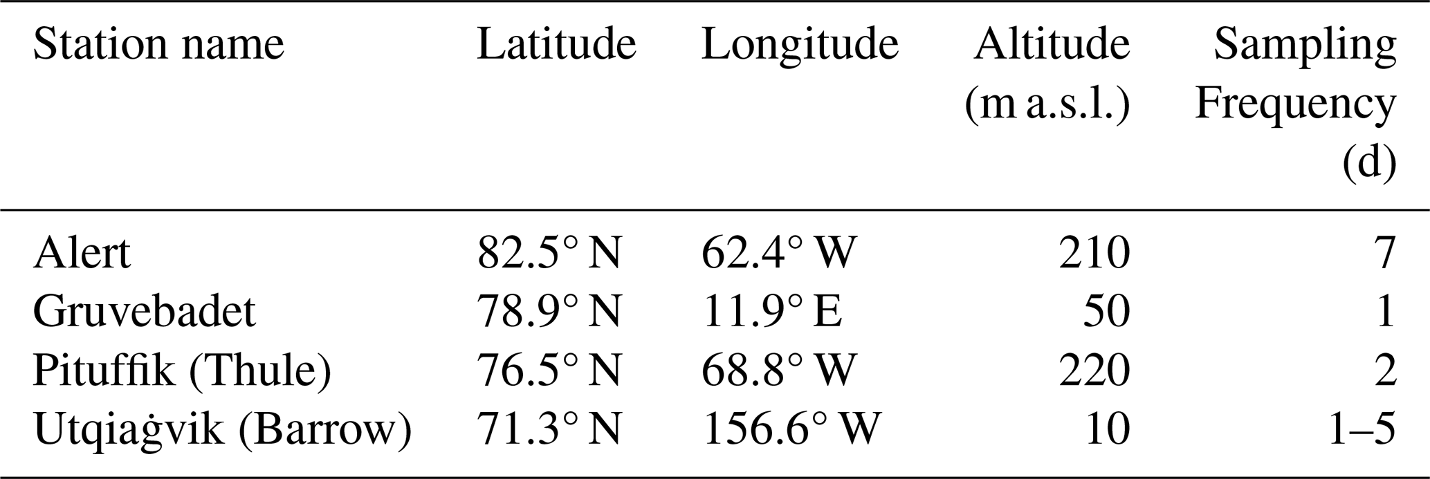
In situ filter samples of particulate methanesulfonic acid (MSAp) were measured at four Arctic stations (Alert, Gruvebadet, Pituffik (Thule), and Utqiaġvik (Barrow)) (Becagli et al., 2016, 2019; Moffett et al., 2020; Sharma et al., 2019). Figure 2a displays the location of each station, and details about each station are given in Table 1. For Alert, Gruvebadet, and Pituffik (Thule), samples from 2010–2017 were used as each site contained sufficient data coverage and a consistent sampling frequency, while for Utqiaġvik (Barrow), samples included 2008–2014 due to data availability and changes in sampling frequency (Moffett et al., 2020). Details about the analytical instrumentation and methods are described in Supplement Text S1. While there are differences in sampling (different inlet and temporal resolution) and analysis (different ion chromatographs) at each station, these measurements are considered comparable as an analysis by two different laboratories for samples from Alert in 2018 showed good agreement (Moschos et al., 2022), and ion chromatography is a reproducible methodology (Xu et al., 2020).
2.1.2 ERA5
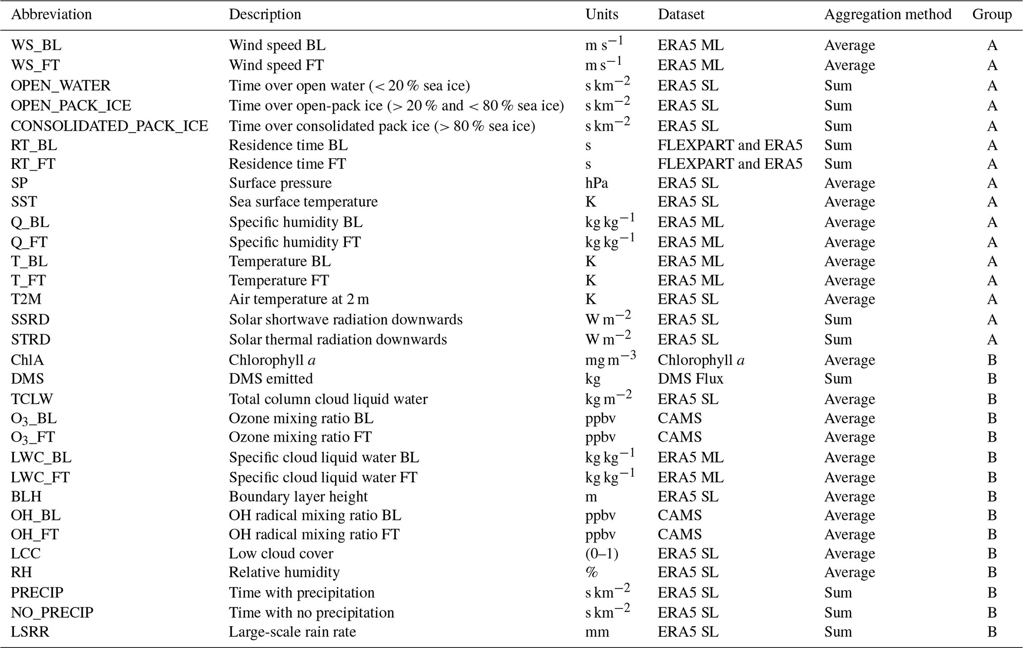
ERA5 is the fifth-generation atmospheric reanalysis product from ECMWF (Hersbach et al., 2020), based on the Integrated Forecast System (IFS) cycle 41r2 numerical model. In this study, ERA5 data on a 0.5° × 0.5° resolution for north of 45° N and every third hour were used to match the geographical extent and temporal resolution of the output derived from the atmospheric transport model FLEXPART (Sect. 2.1.3). Surface-level (SL) and vertically resolved ERA5 data on model levels (ML) were used. The height of each model level on each grid cell was converted to geopotential height using the vertically resolved temperature and specific humidity as well as the logarithm of the surface pressure and the surface geopotential. Relative humidity was calculated using 2 m air temperature and dew point temperature following the method of Pernov et al. (2024a). Here we use ERA5 data from 1 April to 30 September for 2008–2017. Recently, ERA5 surface level variables were compared against continental ground-based stations spanning at least 1 decade for most sites. Overall ERA5 performed well for temperature, solar radiation, and pressure although less so for relative humidity and wind speed/direction (Pernov et al., 2024a). ERA5 is one of the best reanalysis datasets for reproducing precipitation (Loeb et al., 2022) and has shown skill in reproducing precipitation for various regions (Bandhauer et al., 2022; Beck et al., 2019) as well as for the Arctic (Handong et al., 2021). Overall, these limitations should not affect the use of ERA5 or our interpretations. The ERA5 variables were selected based on domain knowledge of the atmospheric conditions which could plausibly affect DMS emission, oxidation to MSA, and removal of MSA aerosols. These include oceanic variables such as sea ice concentration (used to filter ocean biology features; see below) and sea surface temperature; physical atmospheric variables such as wind speed (WS), temperature at the surface (T2M), boundary layer (T_BL), free troposphere (T_FT), shortwave and longwave downwelling radiation (SSRD and STRD, respectively), and boundary layer height (BLH); and hydrological atmospheric variables such as relative humidity (RH), specific humidity (Q), low cloud cover (LCC), large-scale rain rate (LSRR), total column cloud liquid water content (TCLW), and specific cloud liquid water content (LWC). Table 2 lists more details about the ERA5 variables used in this study.
2.1.3 FLEXPART
Air mass residence times were simulated with the Lagrangian particle dispersion model FLEXPART v9.1 (Pisso et al., 2019), driven with meteorological data from the ERA5 reanalysis with 0.5° × 0.5° resolution and 137 vertical levels available every three hours. ERA5 data for FLEXPART were obtained using the Flex extract package (Tipka et al., 2020). A total of 50 000 passive air tracer model particles, representing a passive air tracer without removal processes, were released every 3 h at each of the atmospheric observatories and tracked for up to 10 d backward in time with an output frequency of 3 h. The vertical limit of the FLEXPART output was 15 000 m. For Alert, Pituffik (Thule), and Utqiaġvik (Barrow), a release height of 10 m above ground level (a.g.l.) was used. For Gruvebadet, to account for the complex topography, a range of 10–100 m a.g.l. was used as the release height. The main output from FLEXPART consists of 3-dimensional fields of residence time in units of seconds (s). In contrast to Eulerian models, Lagrangian dispersion models can be applied in time-reversed mode and are superior in representing plumes emerging from point releases (Pisso et al., 2019). However, the quality of their results can be limited by the offline nature of the coupling to meteorological fields, which are restricted in spatial and especially temporal resolution (Brioude et al., 2013). The FLEXPART output was combined (Sect. 2.2) with other data sources for calculating additional input variables for the data-driven models. FLEXPART residence time was combined with boundary layer height from ERA5 to calculate the residence time air masses within the boundary layer (RT_BL) or free troposphere (RT_FT). Sea ice concentrations from ERA5 were combined with FLEXPART to calculate the residence time of air masses over open water (OPEN_WATER, sea ice concentration < 20 %), open-pack ice (OPEN_PACK_ICE, > 20 % and < 80 %), and consolidated pack ice (CONSOLIDATED_PACK_ICE, > 80 %), which was normalized by the grid cell area to give units of s km−2. The precipitation type from ERA5 (no precipitation, rain, freezing rain, snow, wet snow, mixture of rain and snow, ice pellets) was combined with FLEXPART to calculate the residence time of air masses experiencing no precipitation (NO_PRECIP) or precipitation (sum of the amount of time air masses experienced any precipitation types, PRECIP), which was normalized by the grid cell area to give units of s km−2.
2.1.4 CAMS
The Copernicus Atmosphere Monitoring Service Re-Analysis dataset (hereafter referred to as CAMS) is the latest reanalysis product produced by ECMWF, including three-dimensional fields of meteorological variables, chemical, and aerosol species for the period from 2003 onwards. CAMS data were obtained from the Copernicus Atmospheric Data Store (ADS) (https://ads.atmosphere.copernicus.eu/, last access: 8 November 2022). CAMS is based on the ECMWF's IFS CY42R1 cycle and the 4D-VAR data assimilation system (Inness et al., 2019) and uses an extended version of the Carbon Bond 2005 (CB05) tropospheric chemical mechanism (Flemming et al., 2015). Emissions consist of MACCity (MACC and CityZEN EU projects) anthropogenic emissions (Granier et al., 2011), GFAS (Global Fire Assimilation System) fire emissions (Kaiser et al., 2012), and MEGAN2.1 (Model of Emissions of Gases and Aerosols from Nature) biogenic emissions (Guenther et al., 2006). The CAMS data have a spatial resolution of 0.75° × 0.75° with 60 hybrid sigma–pressure (model) levels (13 levels between approximately 400 and 100 hPa) in the vertical (top level at 0.1 hPa) and a temporal resolution of 3 h. The two oxidants, ozone (O3) and the hydroxyl radical (OH) in the boundary layer and free troposphere, were used from CAMS as they are related to the gas- and aqueous-phase oxidation of DMS and its intermediates to MSA (Barnes et al., 2006a). CAMS output of MSAp was extracted using the nearest grid cell to the stations' location (Table 1) for the lowest level and converted from mass mixing ratio to mass concentration using the ambient temperature and pressure from CAMS for comparison to numerical models. CAMS output of MSAp was not included in the data-driven models. To match the spatial resolution of different datasets, re-gridding, using bilinear interpolation from the xESMF (v0.8.2) Python package (Zhuang et al., 2023), was applied to the FLEXPART dataset to match the CAMS spatial resolution.
2.1.5 Chlorophyll a
Chlorophyll a (ChlA) is commonly used as a proxy for phytoplankton biomass and oceanic productivity (Arnold et al., 2010; Huot et al., 2007) and was included for that purpose in this study. Level 3 datasets of satellite-derived daily surface chlorophyll a concentration with a spatial resolution of 4 km from the European Space Agency's GlobColour Project3 (https://www.globcolour.info/, last access: 1 October 2022) were obtained from the Copernicus Marine Environment Monitoring Service (CMEMS4). This product is produced by reprocessing the merged observations from five satellite radiometers (OLCI from Sentinel 3a and 3b, MODIS on Aqua, and VIIRS from Suomi-NPP and JPSS-1); therefore missing data due to the presence of clouds are minimized. The GlobColour dataset is a common and suitable choice for investigating phytoplankton (Ardyna et al., 2017; Becagli et al., 2022; Cole et al., 2015; Xi et al., 2020). The ChlA datasets were re-gridded using bilinear interpolation (xESMF v0.8.2 Python package, Zhuang et al., 2023) to match the 0.5° spatial resolution of FLEXPART.
2.1.6 DMS flux
Oceanic emissions of dimethyl sulfide (DMS) were used to evaluate the ocean–air exchange of DMS and were downloaded from the Copernicus ADS web page (https://ads.atmosphere.copernicus.eu/cdsapp#!/dataset/cams-global-emission-inventories?tab=overview, last access: 15 September 2022) and were not calculated offline for this study. DMS is the initial precursor for MSA formation; therefore, information on its oceanic emission is central to investigating processes related to MSA variation. The estimation of oceanic DMS emissions to the atmosphere requires DMS concentrations in the ocean as well as meteorological variables, specifically the u and v components of 10 m wind speed, as well as the sea surface temperature. The oceanic DMS concentrations used for the flux estimation were provided by Lana et al. (2011). The data are derived from numerous measurements obtained for the period 1989–2009 and were obtained from the Surface Ocean Lower Atmosphere Study (SOLAS) web page (https://www.bodc.ac.uk/solas_integration/implementation_products/group1/dms/, last access: 15 September 2022). It should be noted that these oceanic DMS concentrations are based on a monthly climatology. Formulas for the calculation of the DMS flux were provided by Nightingale et al. (2000). Meteorological data computed by the Norwegian Meteorological Institute using the ECMWF-IFS model version Cy40r1 were used. The daily mean emission data are provided on a regular longitude–latitude grid at 0.5° × 0.5° resolution for the period 2000–2018.
2.2 Feature engineering: residence-time-weighted average of environmental variables
For our data-driven modeling efforts, we engineered appropriate input features to capture the air mass history (environmental conditions and surface interactions) in a time-resolved manner, i.e., capturing the environmental conditions where an air mass was actually located for different intervals backward in time. To create a time-resolved air mass history, FLEXPART residence time and environmental variables from the datasets described in Sect. 2.1 were combined. A total of five time steps backward in time was selected as the duration of the air mass history: as the lifetime of DMS in the atmosphere is approximately 2 d (Breider et al., 2010; Lundén et al., 2007), this can account for the emission and oxidation of DMS and the detection of MSA at the ground-based stations. Daily intervals were selected as the temporal resolution of this air mass history as a compromise between a high-enough time resolution to capture physical and chemical processes and the number of input features in our models. We also selected daily resolution for the time-resolved air mass history to match the highest sampling frequency (daily at Gruvebadet). For each variable and observation, we calculated aggregations for daily intervals (up to five daily time steps before release time) backward in time as indicated in Table 2. For the vertically resolved environmental variables (ERA5 and CAMS), the geopotential height of each grid cell was calculated according to the ERA5 documentation using temperature, surface level pressure, and geopotential height (IFS Documentation CY41R2, 2024). This geopotential height of each grid cell was compared to the boundary layer height from ERA5. Grid cells inside the boundary layer were averaged to create a boundary layer average of the environmental variables. Grid cells above the boundary layer height were averaged up to the ERA5 model level corresponding to the highest non-zero FLEXPART level to create a free troposphere average of the environmental variables. The residence time in the boundary layer and free troposphere was calculated by summing the FLEXPART residence time over all longitudes and latitudes for grid cells below or above the boundary layer height, respectively. The relative residence time (boundary layer or free troposphere) was calculated by normalizing the FLEXPART residence time in each grid cell to the sum of FLEXPART residence times over all grid cells and was applied to the boundary layer and free troposphere separately. To account for different sized grid cells, the relative FLEXPART residence time was weighted by the area of each grid cell (grid-cell-area-weighted relative residence time). The grid-cell-area-weighted relative residence time was used to calculate a weighted average of the environmental variables. In this manner, we could ascertain the environmental conditions while accounting for where air masses actually were, directly accounting for transport at our locations of interest. A schematic for the feature engineering procedure is displayed in Fig. 1 using SSRD at Gruvebadet on 1 June 2010 as an example.
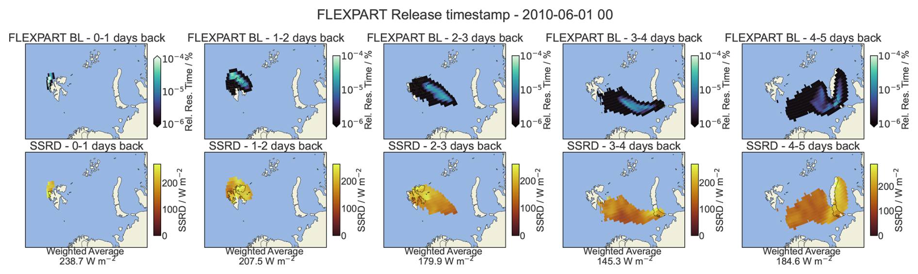
Figure 1Schematic of the feature engineering process. The top row represents the relative FLEXPART boundary layer residence time, and the bottom row shows the average surface solar radiation downwards (SSRD, Table 1) for the different daily intervals backward from 1 June 2010 00:00 UTC for Gruvebadet. Calculating a weighted average of the SSRD using the relative residence time as weights results in the weighted average listed below each SSRD subpanel.
2.3 Preparation of input data
Measurements of MSAp at the ground-based stations varied in terms of frequency and regularity, while the feature-engineered variables (described above in Sect. 2.2) were initially processed at hourly resolution for every third hour (the temporal resolution of the FLEXPART output). The variables therefore needed to be temporally aggregated to match the station measurements. The aggregation was done over non-overlapping time windows corresponding to the sampling periods of each installed aerosol filter. For this aggregation, some features were summed, while others were averaged, according to the physical nature of each variable and how it relates to MSA formation/removal (see Table 2 for more details). For instance, time over open water (OPEN_WATER) was summed as the total amount of time air masses spent over open water is more informative than an average, whilst for the 2 m temperature (T2M), a sum is not physically meaningful; therefore an arithmetic mean was applied. LSRR (originally expressed as mm d−1 in ERA5) was summed over the daily intervals to give units of millimeters. Total DMS emission is originally expressed as kg m−2 s−1. During the feature engineering procedure, the time unit was converted to days; the area unit was converted to km−2; and the emission was summed over the daily intervals, normalized to the grid cell area, and summed over all grid cells for a given daily interval to give units of kilograms (which was then summed over the filter collection period).
The four stations only measure MSAp concentrations locally; therefore, models were first trained and tested on the specific stations individually, as indicated by “St” throughout the text. To model pan-Arctic MSAp, we created two additional datasets to train our models. The first one is called All Stations Full (ASF), which is simply the merger of all data from the four stations. For this, the stations' geographical coordinates were not used: stations were implicitly considered independent replicates (in a statistical sense) if they had data on the same day. The second additional dataset is called All Stations (AS), which is another merger of a subset of data from the four stations: we sub-sampled measurements from the stations with higher temporal frequency (e.g., Gruvebadet with mostly daily measurements) to match those of the lowest temporal frequency (Alert, with roughly weekly measurements). Therefore, in AS all four stations are represented equally in terms of the number of observations.
The feature engineering presented in the previous sections produced a large number of variables we could include in our models as predictors. The different data sources also had varying degrees of accuracy and reliability. We therefore manually subset the features into two groups, denoted as Group A and B. Group A included the variables that we deemed to be the most related and reliable among the predictors of MSAp, using domain knowledge of atmospheric chemistry and physics. For instance, surface air temperature affects the oxidation pathways of DMS and the thermodynamic phase of water in the atmosphere. Furthermore this variable is well reproduced by ERA5 in the Arctic (Pernov et al., 2024a); hence it was included in Group A. Group B includes features which were expected to be good predictors for MSA, although the accuracy of these variables may be lower in the areas covered by our study. For instance, measurements of hydroxyl radical mixing ratios (OH) are analytically challenging and datasets are sparse (Lelieveld et al., 2016; Stone et al., 2012); therefore CAMS cannot be validated against sufficient in situ observations, especially in the Arctic. Hence it was included in Group B. DMS flux is based on a monthly climatology of seawater DMS concentrations (Lana et al., 2011); therefore, short-term variations depend only on parameterizations based on wind speed and sea surface temperature. Hence was included in Group B. Table 2 lists all features in Groups A and B. Table A1 lists commonly used abbreviations throughout this paper.
2.4 Model evaluation
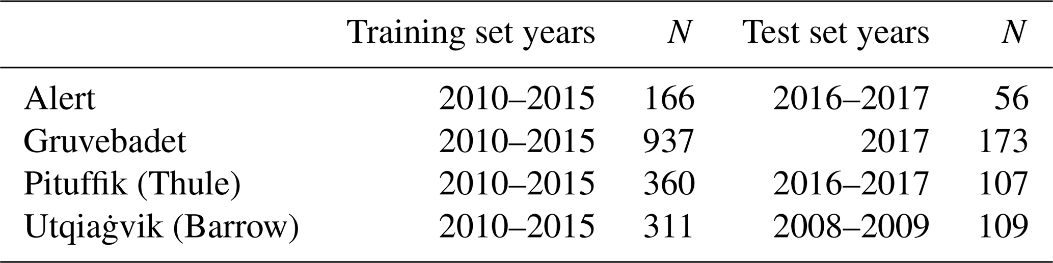
We evaluated our models by assessing the out-of-sample prediction error. To this end, we first performed a training–test split: for every station, we left out some observations corresponding to one or two summers, before attempting any modeling (Table 3). These were our test subsets, and they were used to assess prediction error as a last step for the final versions of the models presented below. The remaining data are our training subsets on which we applied a temporal cross-validation (CV) scheme. This CV scheme was mainly used for hyperparameter tuning for the baseline models (see Sect. 2.6.1) and was the criterion in the feature selection procedure for the additive model (see Sect. 2.6.2). We used a 6-fold CV, corresponding to leaving out 1 year of data from the training set (between 2010 and 2015; see Table 3) for each station. Thus, data spanning 5 years were used for fitting the models, and out-of-sample prediction could be performed on the 1 year of data in the left-out fold. Details about both training and test data for all stations are summarized in Table 3. Among other accuracy metrics, the CV-based mean squared error (MSE) was computed as an average over the 6 folds. MSE is defined by Eq. (1):
where yi is an observation, is the prediction of the model on this data point (from either RF or AM), and n stands for the number of observations in a given fold for a given station. MSE values lie within [0, ∞], where a value closer to 0 represents better predictions (lower error). Another two important metrics we report are the prediction coefficient of determination (or R2 value) as defined by Eq. (2):
where denotes the mean of the observations in all other folds for a given station (constant prediction). We also report the Pearson (linear) correlation coefficient (PCC) as defined by Eq. (3):
where denotes the mean of the predictions. Note that the R2 can take values within (−∞, +1]: a value of 0 means that the model prediction is equivalent to the average of the MSA values in the training set, a negative value means that the model predictions are worse than this average, and a value closer to 1 means that the model predicts better than the training set average (a value of 1 meaning perfect prediction). It should be noted that the R2 metric we use in this study is not the square of the PCC. The PCC is calculated using the stats module from the Python package scipy.
We compute all metrics on two scales: the original scale of values and the natural logarithm scale, the one used to train the models. The purpose of training the models and assessing their prediction on the log scale as well is that large observations are compressed by the transformation; thus squared errors on the log scale may be more informative for the majority of the observations (i.e., less sensitive to potential outliers). The same metrics were also computed on the test set.
Table 2Key details of the features used for data-driven modeling of MSAp. Variables for the boundary layer and free troposphere are denoted by “BL” and “FT”, respectively. ERA5 data on surface and model levels are denoted by “SL” and “ML”, respectively. For the Aggregation method column, “Average” indicates the arithmetic mean.
2.5 Imputing missing values
Missing data for both the in situ MSAp measurements (target variable) and for the input variables (features) exist and potentially could affect or bias our analyses. Regarding the in situ MSAp measurements, we considered the station-specific aerosol filter collection duration (called hereafter nominal resolution) as a reference over which features were aggregated. These nominal resolutions were daily for Gruvebadet and Utqiaġvik (Barrow), every 2 d for Pituffik (Thule), and every 7 d for Alert. Based on a trial-and-error approach, we decided to enforce the rule that any sequence of consecutive missing values longer than 3 times this nominal resolution would be deemed too long to be imputed without introducing artifacts. These long patches were thus left as is, and features were aggregated over time windows according to the nominal resolution. Shorter sequences of consecutive missing values were imputed at the nominal resolution. For Gruvebadet and Pituffik (Thule), this was done by linear interpolation using the two closest available measurements. For Utqiaġvik (Barrow), the variable temporal resolution depending on the time of year (Table 1) complicated this procedure, and gaps of 3 and 4 d occurred too often for our rule to be applied strictly at a daily nominal resolution. Here we left gaps up to 5 d (as these could be valid measurements) as is and imputed by linear interpolation based on the two closest values to those gaps lasting between 5 and 10 d. Finally, Alert required more care, as missing values could last for long periods (> 3 weeks), making linear interpolation unreliable. Here, we used different imputation methods for short gaps (up to two missing values) and long gaps (3-weekly values missing), targeting at most 10 d between values. For short gaps, we used local quadratic fits, fitted by minimizing the sum of squared residuals on the natural logarithm scale. We used neighborhoods of three available values before and after the gaps, weighted by a Gaussian kernel. For the single long gap, we used a model with a polynomial of degree 5 representing long-term time trends and yearly seasonality represented by a linear combination of cubic B splines, also fitted by minimizing the sum of squared residuals on the log scale. Figure S14 illustrates the imputation of such short and long gaps for Alert in situ measurements.
Regarding the input feature, ChlA, to minimize the impact of short gaps due to clouds or the presence of sea ice, we studied different data imputation strategies. We first assessed seven different algorithms (mean, median, imputeTS (Moritz and Bartz-Beielstein, 2017), k nearest neighbor, principle component analysis, and MissForest) based on randomized masking of measurements for Alert and measured the reconstruction error over the imputed values. Within the feature set, there are strong correlations that can be exploited to fill measurements. We found that MissForest (Stekhoven and Bühlmann, 2012) was the best-performing method, and we used this to impute values for the entirety of the feature input dataset. MissForest is based on the application of random forests iteratively. First, it imputes missing input data using the mean. Then it trains a random forest regressor on a set of fixed features, to predict missing values on a separate feature to be filled. It proceeds iteratively and stops when the predicted missing values converge or when the maximum number of iterations is reached. MissForest is highly flexible and does not make any assumptions about the data distribution. However, purely statistically driven data imputation might lead to physically implausible values. To achieve consistency, we set all ocean biology variables (DMS and ChlA) to 0 if the sea ice concentration from ERA5 was > 80 % as no ocean–atmosphere exchange is expected for these conditions. For each station, measurements below the reported limit of detection were imputed with half the detection limit (Becagli et al., 2016, 2019; Moffett et al., 2020; Sharma et al., 2019).
Table 3Train–test splits for all stations. N is the number of observations in each set.
2.6 Data-driven models
For this task, we considered non-linear regression models approximating the log-transformed target, MSAp concentration, plus a constant as , for , where N is the sample size (different for each station, Table 3). Our choice of log transformation and addition of a constant was based on achieving a somewhat symmetrical target distribution, which is better suited when using a mean squared error loss function, as well as improving numerical stability in the optimization. All models make use of the same engineered features presented above as inputs to predict Y. We considered two main approaches for modeling these relationships. The first is a “baseline model” composed of a common random forest (RF) regressor (Breiman et al., 1984), which is a standard and well-accepted regression model, also offering some insights on feature importance. We also developed a specific additive model (AM), which models the temporal relationships across the features and the target in a more principled manner while providing a more interpretable model overall. The interpretability of estimated effects in the AM is a key aspect here and the main reason that we developed it. The goal is to identify drivers and describe their relation with the target variable while at the same time to have full control over the optimization process and variable selection procedure. We present the baseline RF model and its setup in the following Sect. 2.6.1 and the AM in Sect. 2.6.2. Other modeling approaches were explored; we summarize their performance in Supplement Text S2 and Fig. S1. These other approaches were not retained because their predictive performance was no better than that of RF and AM. In the case of similar performance, RF and AM still had interpretability benefits, notably in identifying which features contributed the most to the model prediction power, and thus were the ones we retained.
2.6.1 Baseline model: random forest
Random forests (RFs) are among the top-performing models in a wide variety of classification and regression tasks and are known to be robust to overfitting while being fast to train and fast at inference (Biau and Scornet, 2016). RFs are often a nominal selection for most data-driven applications. RFs are composed of an ensemble of decision trees, where each tree is trained on a random subset of data (a bootstrap) and by testing a random subset of features for each decision tree node optimizing an impurity measure. Averaging the output of each trained tree allows the RF to predict a given input data point. In addition, RFs provide an implicit ranking of features, which for regression tasks is based on the average reduction in the squared error at node splits for a given feature, which we will refer to as an importance score. Although ranking features according to their explicit relationship with the target variable is a difficult problem, RFs provide a simple yet effective way to sort features from more to less important. This will be used to qualitatively compare with the selected features based on our proposed AM described in Sect. 2.6.2.
For each experiment with RFs, we performed a grid search for the depth of each tree and for the minimum number of data points per node to make it a leaf. Those two hyperparameters control how much each tree in the random forest can grow, trading off training accuracy for speed as well as avoiding overfitting. The number of trees was set to 500 and kept constant for all the experiments; a larger number of trees did not result in better models but only in increased computational time.
We selected the most important features for the RFs using a method analogous to the additive model forward selection procedure described in Sect. 2.6.2. First, for each of the 500 trees in each RF model, the list of features with a model importance score ≥ 5 % of the maximum importance score for that tree was found. We then took the summed importance scores for each feature across all trees in which they were selected and divided them by the total number of trees (500) to estimate the mean score of each feature only from the trees where it was selected. If this mean score was ≥ 5 % of the mean of the maximum importance scores for each tree, the feature was selected for that model. Re-training the RF with only the selected features did not materially change its predictive performance; see Fig. S1.
2.6.2 Additive model
To maximize predictive performance while retaining interpretable feature effects we developed an additive model (AM) (Buja et al., 1989; Hastie and Tibshirani, 1990). This assumes that the mean of the log-transformed MSA Y is linked to the features by smooth (non-linear) functions. As these functions are unknown, we approximate them by linear combinations of user-specified basis functions. To this end, we used the standard cubic B splines as bases (de Boor, 2001). The ith aggregated value of the kth feature is denoted by xi,k, for , where K is the number of features used in the model (the maximum being K=80 for Group A and K=155 for Group A + B). The cubic B-spline basis function is generically written as B. The AM main equation can be expressed according to Eq. (4):
where α0 is an intercept, J is the number of spline bases we use for every feature effect represented by the linear combination , the αj,k values denote coefficients weighting the different spline bases for the kth feature effect, and εi is an independent error term assumed to have mean zero and constant variance. To reduce the computational cost and as an indirect regularization (see below), we set J=5 throughout. This implies that the spline function relies on knots; these were set as the minimum, median, and maximum observed values for each feature. There are thus 1) + 1 free model parameters. These were estimated on the training data by minimizing the mean squared error (Eq. 1). The mean squared error loss function relies on the assumed independence between the values of εi. Even though the MSA measurements were recorded sequentially in time, with the possibility of temporal dependence (autocorrelation), we believe the independence assumption is tenable here. The rationale is that if the K features include a subset of relevant variables that explain and predict Y, then all that remains is indeed white noise represented by ε. In other words, we assume any (marginal) temporal dependence in Y is captured by the effect of the available features.
The main challenge when fitting such a model is that K can be potentially large, leading the number of parameters P to exceed the number of observations N. That is, the AM can easily overfit the training data, with estimated feature effects appearing overly complex (i.e., wiggly) and difficult to interpret. As we want the model to predict out-of-sample observations well, some regularization is required. Typical regularization approaches allow for a large J and involve adding penalties to the mean squared error loss so that many values of αj,k are shrunk towards zero or even exactly set to zero (Wood, 2017). We explored such approaches, notably using effect-specific ridge penalties or a group lasso penalty to select features as part of model fitting, but could not obtain satisfying results. These also came with undue computational overhead involved in part in selecting the penalty/smoothness hyperparameters. We thus opted for a simpler strategy: we set J=5, which is rather small and guarantees on its own that the estimated feature effects are relatively smooth albeit flexible enough. Rather than enforcing some penalty to counteract a large K, we selected features with a forward stepwise selection (FSS) procedure (Hastie et al., 2020). This scheme starts with an empty model, only with the intercept α0, and sequentially adds features based on an objective criterion. Our criterion here is the prediction MSE based on the temporal CV described in the previous section. At each FSS step, the feature that reduces this CV-based MSE the most is selected and kept in the model in subsequent steps. The scheme ends when the MSE reduction is smaller than a threshold of 5 % of the initial reduction from an empty model to a model with one feature. That way, the model never includes too many variables, P remains low relative to N, and we have the guarantee that the selected features are useful in predicting/forecasting MSA observations. This also comes with computational gains, since the independent fits at each step (one for each candidate feature) can be parallelized. After this FSS round, we explored if any pairwise interaction (product of two features) between the selected features was worth including. For this, we applied the FSS in a similar fashion and only kept the most useful interactions with the same 5 % MSE reduction threshold.
In addition to predictions, the AM yields interpretable effects as output. After training, the estimated effect of feature k on the response is calculated similarly to the mean prediction presented above, where all features except the kth are set to their mean observed value. Therefore, only the marginal contribution of the kth feature remains, and this can be represented as a curve, typically represented over a scatter plot of the response plotted against the kth feature. We refer to these curves (and the plots by extension) as “partial effects”. These partial effects can also be constructed for pairwise interactions. In this case, the interaction between features k and l is computed as the mean prediction where all other features except k and l are set to their arithmetic mean. The interaction partial effect plot is then a three-dimensional surface represented as a function of features k and l. The partial effects were calculated using only the training set.
2.6.3 Strengths and limitations of RF and AM
Both RF and AM are non-linear regression models, although they differ in a few key aspects. First, RF's output is the average of predictions from many decision trees which are based on random subsets of the training data and random subsets of features, while AM considers the entire training set at once (i.e., without random subsets). This randomization generally reduces the risk of overfitting (yielding a smaller prediction variance) compared to constructing a single, large decision tree. For AM, the risk of overfitting was minimized by keeping the number of splines bases low (J=5) and enforcing this stepwise variable selection scheme so that the number of parameters P stayed relatively low. In that sense, AM is generally a simpler model than RF. Second, the predictions from decision trees, and thus from RF, as seen as a mathematical mapping from a feature space to a target variable space, are piecewise constant functions. By contrast, the predictions from AM are smooth by design, as they are computed as the sum of cubic splines (with continuous second derivatives). In practice, this means that the predicted target surface from RF looks like jagged stairs, with jumps at feature splits, while for AM this looks like a smooth surface. Finally, the additive structure of AM in Eq. (4) is quite constrained: features have their respective effects, and these add up to a prediction. We considered pairwise interactions but no higher-level terms (e.g., three-way interactions). By comparison, RF inherently can include higher-level interactions, as splits are being added sequentially (i.e., conditioned on previous splits) when growing a decision tree (up to a maximum depth, which we tuned as a hyperparameter). This higher complexity makes RF generally more flexible than AM. Although this flexibility comes at the cost of harder interpretability as one cannot easily visualize the estimated effect of a feature on the target, specifically because of such interactions likely being different from tree to tree within the ensemble. The additive constraint of AM is what makes the estimated partial effects directly interpretable, say, as a curve displayed in a plot.
2.7 Numerical model output for comparison to in situ observations
We compare in situ MSAp measurements from each Arctic station to output from three numerical models (GEOS-Chem, OsloCTM3, and GISS-E2.1) and one reanalysis product (CAMS) to gauge their current predictive abilities. Details about CAMS are given in Sect. 2.1.4, and details about the numerical models are given below. For a quantitative comparison using a regression analysis, we focus on the same evaluation metrics used for evaluating the data-driven models (R2, PCC, and MSE) and limit our evaluation to the same months (April–September), we calculated the slope of predicted versus measured MSAp as an additional metric. For a qualitative comparison, we compare the average seasonal cycles of numerical model output to in situ observations. For both the quantitative and qualitative comparison, we utilize all available years at a given station to obtain as large a sample size (and therefore a more robust statistical analysis) as possible.
2.7.1 GEOS-Chem
Output from the global chemical transport model, GEOS-Chem (v12.9.3: https://zenodo.org/records/3974569, last access: 15 June 2023), for atmospheric concentrations of MSAp for the years 2016 and 2017 was used in this study. Transport processes and cloud properties are driven by NASA MERRA-2 (Modern-Era Retrospective Reanalysis for Research and Applications, Version 2) reanalysis meteorology (Gelaro et al., 2017), which has a horizontal resolution of 0.5° × 0.625°. GEOS-Chem has a 4° × 5° horizontal resolution with 47 vertical levels. The chemical reactions were calculated every 60 min, and the monthly averaged data were produced as model output. Boundary layer MSAp is calculated from GEOS-Chem output of boundary layer height, air density, temperature, and surface pressure. The oceanic DMS emission flux is parameterized using a sea-surface-temperature-dependent and wind-speed-dependent gas transfer velocity (Johnson, 2010) and the climatology of seawater DMS concentrations (Lana et al., 2011; Nightingale et al., 2000). GEOS-Chem contains comprehensive HOx–NOx–VOC–O3–halogen tropospheric oxidant chemistry including recent updates to halogen chemistry and cloud processing (Bey et al., 2001; Holmes et al., 2019; Wang et al., 2019). In addition to the original version of GEOS-Chem v12.9.3, we used the multiphase DMS oxidation chemistry scheme recently developed by Tashmim et al. (2024), while the aqueous-phase reaction of MSA and OH was omitted due to the high uncertainty in its reaction rate (Chen et al., 2018). The wet and dry deposition schemes for aerosols and gas species are based on previous studies (Amos et al., 2012; Liu et al., 2001; Wesely, 1989).
2.7.2 OsloCTM3
The OsloCTM3 is an offline global three-dimensional chemistry transport model with total MSA (gaseous and particulate MSA) and output for 2008–2017 was used in this study. We opted to include this model output even though it was for total MSA as modeled MSAp in the Arctic is scarce, and from measurements of gaseous and particulate MSA from the MOSAiC expedition (Boyer et al., 2023; Heutte et al., 2023; Shupe et al., 2022) the ratio of gaseous to particulate MSA in the central Arctic Ocean is approx. 0.03; thus it would not likely significantly influence the results of this study. OsloCTM3 is driven by meteorological forecast data from the European Centre for Medium-Range Weather Forecasts Integrated Forecast System (ECMWF-IFS) model with a 3-hourly temporal resolution. OsloCTM3 has a 2.25° × 2.25° horizontal resolution, 60 vertical layers, and monthly temporal resolution. The lowest layer was taken as representative of surface concentrations. OsloCTM3 consists of a tropospheric and stratospheric chemistry scheme (Søvde et al., 2012) as well as aerosol modules for sulfate, nitrate, black carbon, primary organic carbon, secondary organic aerosols, mineral dust, and sea salt (Lund et al., 2018). The sulfur cycle chemistry scheme and aqueous-phase oxidation are described by Berglen et al. (2004). The oceanic DMS emission flux in OsloCTM3 is parameterized using wind fields from ECMWF-IFS, gas transfer velocity calculations from Nightingale et al. (2000), and seawater DMS concentrations from Kettle and Andreae (2000). Aerosol removal includes dry deposition and washout by convective and large-scale rain from ECMWF-IFS.
2.7.3 GISS-E2.1
The NASA Goddard Institute of Space Studies (GISS-E2.1) Earth system model (ESM), GISS-E2.1, is a fully coupled ESM; for a full description of GISS-E2.1, see Kelley et al. (2020). GISS-E2.1 has a horizontal resolution of 2° × 2.5° and 40 vertical layers and produced monthly output for 2008–2017. The output of the GISS-E2.1 model used historical CEDS emissions from 2008–2014 and SSP2-4.5 from 2015–2017. The lowest layer was taken as representative of surface concentrations. The tropospheric chemistry scheme used in GISS-E2.1 (Shindell et al., 2001, 2003) includes inorganic chemistry of Ox, NOx, HOx, CO, and organic chemistry using the CBM4 scheme (Gery et al., 1989). The meteorology was nudged to the NCEP reanalysis (Kalnay et al., 1996). The one-moment aerosol (OMA) scheme used (Bauer et al., 2020) is a mass-based scheme in which aerosols are assumed to remain externally mixed and have a prescribed and constant size distribution. The OMA scheme treats sulfate, nitrate, ammonium, carbonaceous aerosols (including methanesulfonic acid formation), dust, and sea salt. The natural emissions of DMS are calculated interactively using prescribed and fixed maps of DMS concentration in the ocean (Im et al., 2021).
This section begins with an analysis of the seasonal cycles and source regions of in situ MSAp observations at the High Arctic stations for context. We then evaluate current numerical models' ability to simulate MSAp, followed by a performance analysis of our data-driven models. The most relevant features selected by the models are discussed, and their effects on the AM output of MSAp are investigated.
3.1 In situ MSA observations from Arctic stations
The locations and seasonal cycles of MSAp at each of the Arctic stations are displayed in Fig. 2a and b, respectively. For all stations, MSAp is elevated beginning in April and ending in September. This period corresponds to polar day, receding sea ice, increase in atmospheric oxidants, and phytoplankton blooms. Details about each station's seasonal cycle and source regions are given below.
Alert, the most northern station located at 210 m a.s.l. on the Canadian Archipelago (Fig. 2a and Table 1), which is surrounded by sea ice and land, experiences air mass transport mainly from the central Arctic Ocean, Canadian Archipelago, and Greenland Sea (Sharma et al., 2012). Alert exhibits a maximum in MSAp during May (0.014 [0.011, 0.021] µg m−3 and a median [25th, 75th percentiles]) followed by lower levels during June and July until reaching a second smaller maximum in August (0.009 [0.006, 0.011] µg m−3). The maximum in May is likely due to efficient transport from regions of biologically active waters in the Northern Atlantic (Sharma et al., 2012; Xie et al., 1999), while the second maximum in August likely arises from biological emissions from regions of retreating sea ice in the Arctic Ocean (Sharma et al., 2019).
Gruvebadet, located on the coast of the Svalbard Archipelago with sea ice to the north and open ocean to the south, experiences air mass transport mainly from the Greenland and Barents Sea (Becagli et al., 2016). Gruvebadet displays the highest MSAp concentrations of all the stations, with a maximum in May (0.022 [0.011, 0.046] µg m−3). As the summer progresses, monthly median MSAp concentrations steadily decrease, although the 75th percentile does display a shoulder in July showing the increased variability of MSAp during the later summer months. The May maximum is likely related to the spring bloom in the Barents Sea, and the variability in the later summer is likely biological activity in the Greenland Sea as well as differences in oceanic DMS-producing species in these regions and timing/location of sea ice retreat (Becagli et al., 2019).
Pituffik (Thule), located in northwestern Greenland at 220 m a.s.l., experiences air mass transport almost exclusively from Baffin Bay (Becagli et al., 2016). Although located close to each other, Pituffik (Thule) experiences similar levels of MSAp compared to Alert but interestingly a different seasonal cycle. From May to July, median MSAp concentrations at Pituffik (Thule) plateau around 0.011 [0.007 and 0.018 µg m−3], while Alert experiences two local maxima (May and August as discussed above). The northern section of Baffin Bay regularly experiences the North Water (NOW) polynya, which is characterized by sea-ice-free areas and upwelling of nutrients (Tremblay et al., 2002). The NOW polynya begins to form in early spring and stays open until late July when sea ice is largely absent from the region. The timing of the NOW polynya and the associated exposure of the underlying ocean to the atmosphere and solar radiation as well as nutrient-rich upwelling (which is crucial for DMS production) are the likely cause of the rather flat MSAp seasonal cycle at Pituffik (Thule) (Becagli et al., 2016).
Utqiaġvik (Barrow), located on the shores of the Beaufort Sea in the North American Arctic, experiences air mass transport from the central Arctic Ocean (Chukchi and Beaufort Seas), the Bering Sea/Strait, and surrounding continental areas (Alaska, Canada, and Russia) (Moffett et al., 2020; Quinn et al., 2002; Sharma et al., 2012). Utqiaġvik (Barrow) displays a different seasonal cycle compared to the other stations (Fig. 2b), with maximum MSAp concentrations occurring in later summer. Utqiaġvik (Barrow) experiences an increasing pattern in MSAp concentration from April culminating in a maximum monthly median during August (0.012 [0.006, 0.016] µg m−3). Interestingly, the maximum 75th percentile (June) at Utqiaġvik (Barrow) is not concurrent with the maximum monthly median (August), which indicates higher variability in June but on average higher values during August. The low values in early spring could be due to the low amounts of biological activity in the surrounding seas (Hulswar et al., 2022; Lana et al., 2011) during this time (as opposed to the biologically active waters in the Northern Atlantic during spring), whilst the late summer peak could be due to transport from more warmer, local waters in the Northern Pacific during August (Moffett et al., 2020; Quinn et al., 2002), which is a hotspot of DMS emission (Wang et al., 2020).
The differences between the stations could be credited to the different locations, sea ice retreat timing/location, differences in the DMS-producing communities, oxidant species and levels, precipitation patterns, and different air mass transport patterns. The differences in the seasonal cycles, environmental conditions, and circulation patterns of these geographically dispersed measurement stations allow for an investigation and modeling of the processes unique to each station from a pan-Arctic perspective. While much research has gone into elucidating the source regions, geographic differences, and seasonal behavior of MSAp, few have investigated the environmental drivers of MSAp, which is one of the goals of this study.
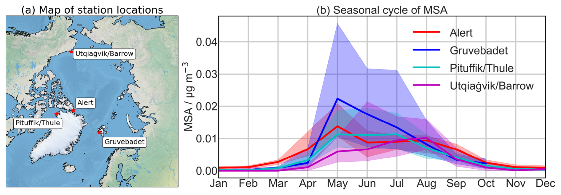
Figure 2Station locations and seasonal cycles. (a) Map of Arctic stations marked with a red star. The map background is from Natural Earth. (b) MSAp seasonal cycle at Alert (red), Gruvebadet (blue), Pituffik (Thule) (cyan), and Utqiaġvik (Barrow) (magenta). The median is represented by the thick lines, and the interquartile range is represented by the shading.
3.2 Comparison of numerical model output to in situ MSA concentrations
For this comparison, our intent is to quantitatively gauge the current level of predictive performance for MSAp in numerical models, especially for the seasonal cycle, and for comparison against our data-driven models. We do not intend to identify and explore the underlying causes of the discrepancies between the numerical models and observations which are beyond the scope of this work. The regression analysis and seasonal cycles of the numerical models against in situ observations for Alert, Gruvebadet, Pituffik (Thule), and Utqiaġvik (Barrow) are presented in Figs. 3, S2, S3, and S4, respectively.
Output from GEOS-Chem was only obtained for 2016–2017; therefore only a comparison at Alert, Gruvebadet, and Pituffik (Thule) was possible. MSAp from GEOS-Chem is calculated over the height of the boundary layer for comparison to observations. For all three stations, a negative R2 value is observed, indicating that GEOS-Chem is worse at predicting MSAp values than the mean of the observations. PCC values range from 0.16 (Pituffik (Thule)) to 0.85 (Gruvebadet), although only 1 year was available for comparison at Gruvebadet (Sect. 2.1.1 and 2.7.1), making this result less statistically robust. MSE values range from 6.27 × 10⁻³ (Alert) to 3.5 × 10⁻² µg m−3 (Gruvebadet) (Figs. 3, S2, and S3). Slopes larger than 1 are observed for all stations, ranging from 1.28 (Pituffik (Thule)) to 6.67 (Gruvebadet), indicating GEOS-Chem overestimates MSAp relative to observations. The seasonal cycle of observed MSAp is best reproduced by GEOS-Chem at Alert, with the model able to capture the double maxima in spring and autumn (Fig. 3), although the timing and relative magnitude of the second peak in autumn are not aligned with observations.
The OsloCTM3 output is available for the entire study period; therefore, all data from all stations could be used. MSAp concentrations from the lowest model level were taken as representative of the surface level. OsloCTM3 overestimates in situ MSAp observations at all locations, with slopes ranging from 3.5 (Pituffik (Thule)) to 6.5 (Gruvebadet). Additionally, the variation and magnitude are poorly reproduced with negative R2 values for all stations. The PCC slightly captures variability with values ranging from 0.18 (Utqiaġvik (Barrow)) to 0.47 (Gruvebadet). MSE values range from 0.013 (Pituffik (Thule)) to 0.066 µg m−3 (Gruvebadet). The month of peak MSAp concentrations is consistently during June in OsloCTM3, which does not reflect the variations in the timing of the seasonal maxima at the various locations. At no station does the model correctly predict the peak month of MSA concentration.
GISS-E2.1 output is available for the entire period and the lowest model level was taken as representative of the surface. The GISS-E2.1 model generally overestimates in situ MSAp at Gruvebadet, Pituffik (Thule), and Utqiaġvik (Barrow) (slopes ranging from 1.63 to 4.2), and the observed variation is poorly captured with negative R2 values and MSE values ranging from 1.78 × 10⁻⁴ (Alert) to 0.014 µg m−3 (Gruvebadet). At Alert, the magnitude of MSAp concentrations is best reproduced by the GISS-E2.1 model compared to other stations as evidenced by the lowest MSE (1.78 × 10⁻⁴ µg m−3), although concentrations are underestimated with a slope of 0.52, and the variation and magnitude are poorly captured with a negative R2 value. PCC values range from 0.19 (Alert) to 0.64 (Gruvebadet). The peak month of MSAp concentration from the GISS-E2.1 model is consistently during June. Several features from the in situ MSAp seasonal cycles are captured by the GISS-E2.1 model, for example, the second, minor peak of MSAp during August at Alert. The peak month of MSAp concentrations at Utqiaġvik (Barrow) is August, and while GISS-E2.1 does not capture this, it does show elevated levels during August. At Pituffik (Thule), the seasonal cycle is quite well captured apart from greatly overestimating concentrations during June. Overall, the GISS-E2.1 model reproduces MSAp concentrations at similar magnitudes to those from in situ observations and can capture certain features of the observed seasonal cycle, although it incorrectly predicts the timing and concentrations during the peak month of MSAp levels.
The CAMS MSAp data were averaged using the median according to the start and stop time of filter samples for the respective stations. CAMS output generally, but only slightly, underestimates in situ MSAp observations, with slopes for all stations ranging from 0.45 to 0.80. The variability and magnitude are poorly captured, with negative R2 values for all stations. The PCC is consistent for each station, with values between 0.3 and 0.4, and MSE values range from 2.1 × 10⁻⁴ (Pituffik (Thule)) to 1.46 × 10⁻³ µg m−3 (Gruvebadet). The absolute values of the seasonal cycle are close to observed values, although the peak MSA month is incorrectly predicted by CAMS at each station. A slight shoulder is observed during May for CAMS MSAp at Alert; however, no other noticeable features of the in situ seasonal cycle are reproduced. Overall, the CAMS reanalysis product most accurately reproduces the levels, seasonal cycle, and spatial distribution of MSAp in the Arctic, although it does not reproduce the timing of peak MSA concentrations.
In summary, we find that, in general, numerical models struggle to accurately reproduce the variability, magnitude, and seasonal cycles of in situ MSAp observations. GEOS-Chem, GISS-E2.1, and OsloCTM3 overestimate MSAp levels and miss the timing of peak MSA concentrations. CAMS is generally able to reproduce MSAp levels with a similar magnitude to observations, although the seasonal cycle is usually inconsistent. Although CAMS was able to most accurately reproduce the behavior of MSAp, it will not be able to predict long-term future concentrations for climate analysis, being a reanalysis product capable of only short-term forecasting. Therefore, our science community still lacks the appropriate modeling tools to accurately explore the climatic importance and future changes of MSAp.
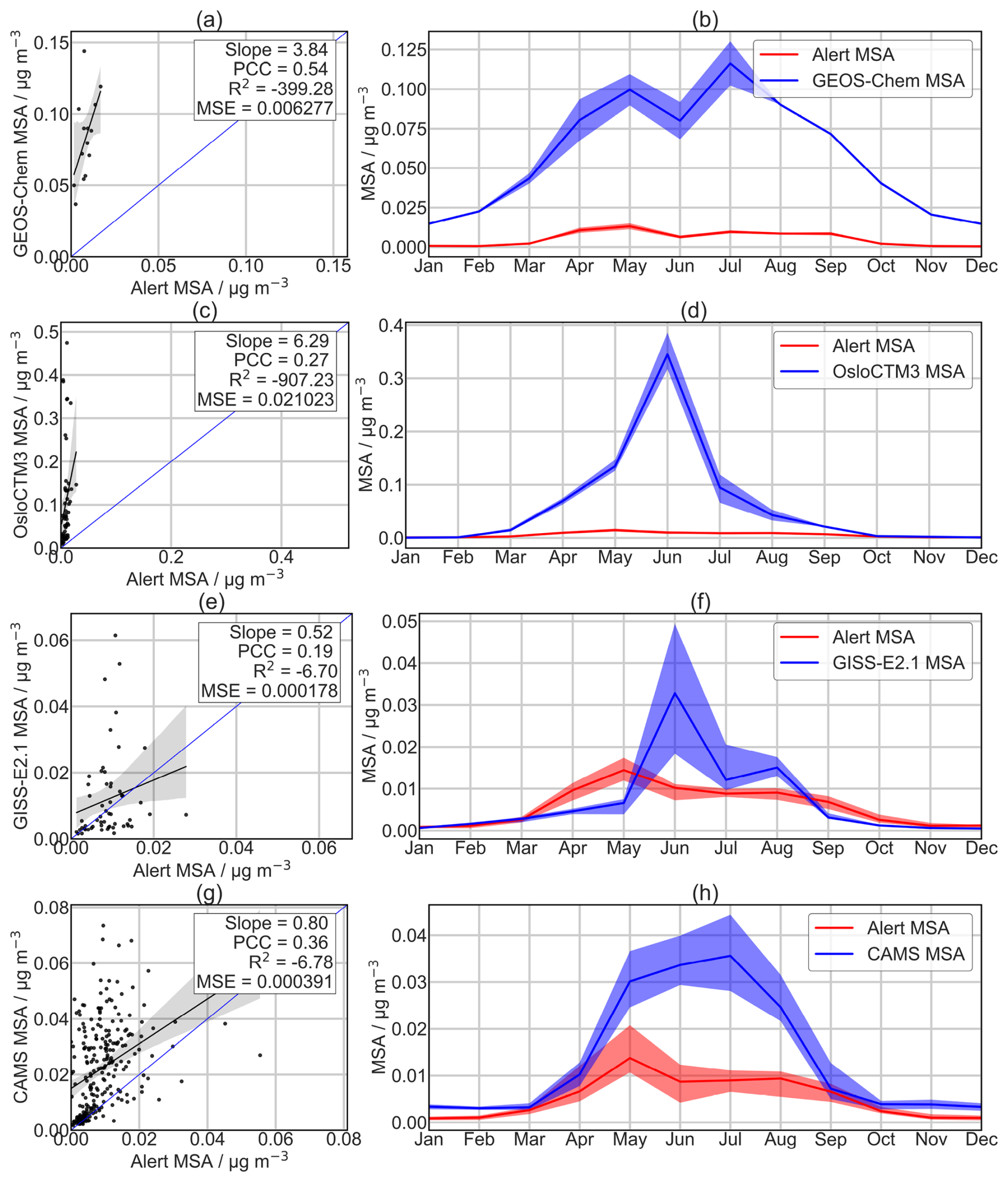
Figure 3Comparison of modeled against in situ MSAp observations from Alert. Scatter plots on the left compare only April to September (over the available period for each station) with the 1:1 line in blue, linear fit in black, 95 % confidence intervals estimated through bootstrapping in the shading, and seasonal cycles on the right (thick line is the median and shading is interquartile range) for GEOS-Chem (a, b), OsloCTM3 (c, d), GISS-E2.1 (e, f), and CAMS (g, h). The MSE, R2, and PCC values are calculated according to Eqs. (1), (2), and (3), respectively.
3.3 Data-driven model performance
In this section, we present and discuss the implemented data-driven models used to estimate ambient MSAp concentrations. We use RF as a baseline model and focus on AM as a tailored model developed for the task at hand. Figure 4 summarizes the prediction performance in the temporal CV scheme and on the test set (Table 3) for the RF and AM with Group A + B on the four stations. The R2, PCC, and MSE metrics are computed on the MSAp original scale in Fig. 4a and c and on the log scale in Fig. 4b and d, respectively.
Prediction performance is relatively good on the log scale, with R2 values up to 0.49 and 0.54 and PCC up to 0.74 and 0.82 for the temporal CV and test datasets, respectively. Comparing the two models, AM has systematically higher CV R2 (correspondingly lower MSE and similar PCC) in the St evaluations. This is expected since its variable selection procedure was designed to minimize the CV-based MSE. In the AS and ASF evaluations, neither model seems to clearly outperform the other. The R2 values on the original MSAp concentration scale are lower than on the log-transformed data, with a maximum of 0.37 and 0.29 for the temporal CV and test datasets, respectively. A likely explanation for the better performance on the log scale could be the inter-annual, short-term variations in MSAp concentrations, which tend to be underpredicted by the models, particularly affecting the original scale data (Figs. 5 and S6), but less so for the log-transformed data which the models were trained on. The underprediction of MSAp peaks is particularly noticeable for Gruvebadet, where R2 values on the log-transformed data are much higher than for the original data (Fig. 3c and d). Scatter plots and regression lines of the measured versus modeled MSAp are displayed in Fig. S7. The regression lines for RF and AM against observations often overlap or have similar slopes, but with a slight vertical shift particularly evident for Utqiaġvik (Barrow), indicating that different models are producing different amounts of background MSAp for this station. Comparing the left side of Fig. S7 with the right side, the log transformation clearly facilitates model fitting as mentioned above, especially for Gruvebadet (Fig. S7b and f).
Our two data-driven models are relatively complex and rely on a large number of features for this prediction task. However, the results suggest that our models might be missing important variables or critical relationships that are not captured due to either inaccuracies in the original datasets (ERA5, CAMS, FLEXPART, etc.) or an effect of the feature engineering (averaging over daily intervals smooths out short-term temporal/spatial variation or important processes are occurring on timescales further backward in time than 5 d). For instance, models underpredict high observations of MSAp, which could be due to large DMS emissions not being captured in the input features due to either being based on a climatology of seawater DMS (Lana et al., 2011; Nightingale et al., 2000) or occurring further back in time than 5 d. The models also overpredict low MSAp observations, which could be due to extreme precipitation events not being captured by ERA5 (Loeb et al., 2022) or being smoothed out in the feature engineering procedure. Although the summation was used as an aggregation method for precipitation, smoothing over 1 d should not affect extreme events (Table 2). In addition, interannual variability can cause seasons in some years to be markedly different than in other years, making the out-of-sample prediction quite challenging for low-time resolution datasets of 8 years. This is exacerbated by splitting the dataset into training and test sets, which further reduces the number of available data for the algorithm to learn from the data, although this is an essential step in data-driven modeling. The best MSE values on the original data scale are found with the AM for Alert and Pituffik (Thule), whereas the results on the log scale are clearly best at Gruvebadet (Fig. 4c and d). The better performance for Gruvebadet, with a daily temporal resolution, can likely be explained by its training sample size (N=937) being roughly 3 to 6 times larger than that of the three other stations, highlighting the importance of high temporally resolved data. On the original MSA scale, Alert shows the lowest prediction performance, with Utqiaġvik (Barrow) being a close second. Alert, with weekly temporal resolution, has the smallest training sample size (N=166), again hinting at the importance of having enough observations to achieve better prediction. The modeled MSAp values from RF and AM show similar temporal patterns relative to the observations for the test set years (Fig. 5), although capturing both the timing and magnitude of peaks and troughs is difficult, and often only one of the two is captured at a time (i.e., either the magnitude or timing is predicted correctly but not both).
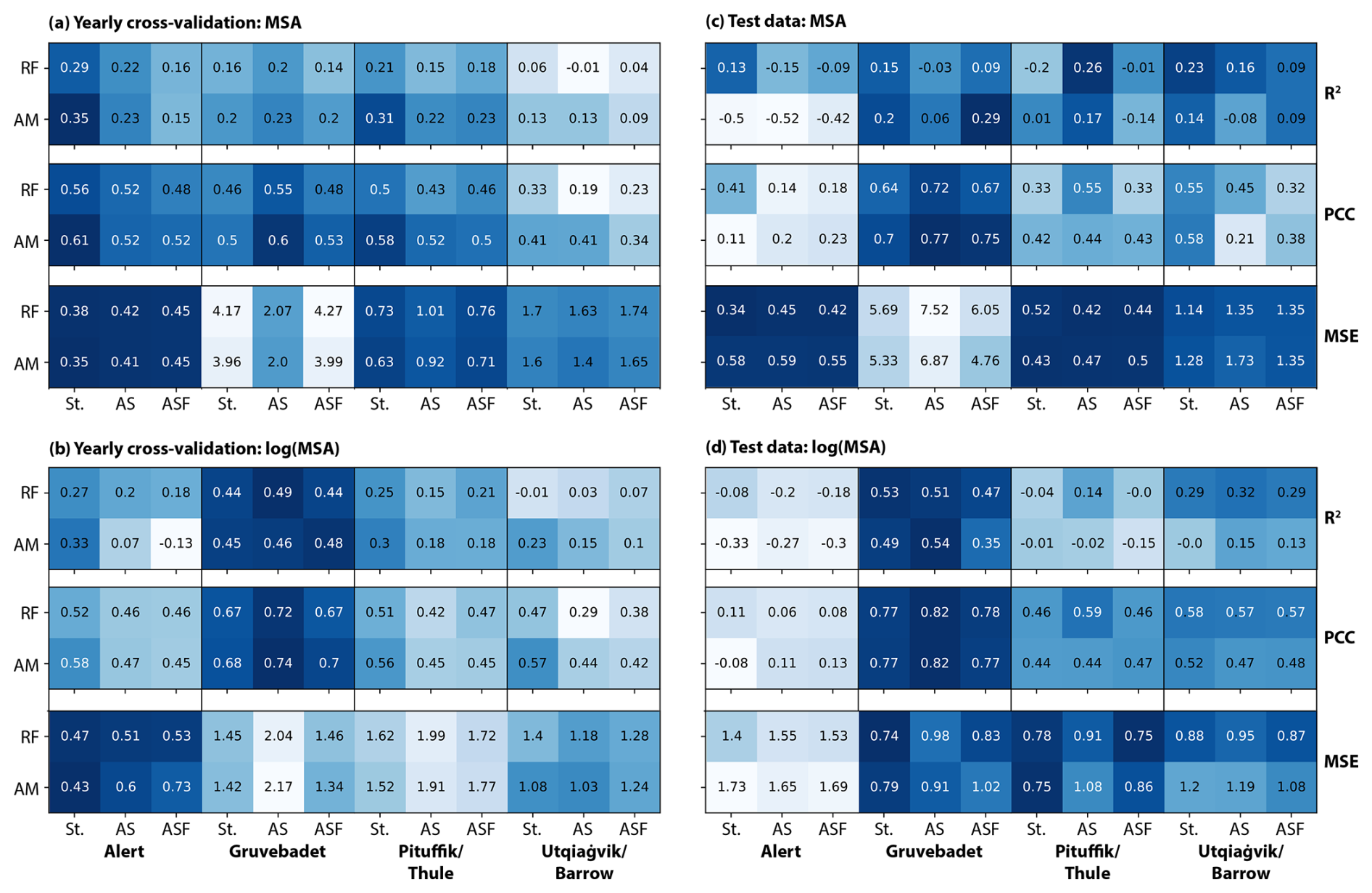
Figure 4Prediction performance for the temporal cross-validation (CV) scheme and on the test set for the four stations, using the selected features from Group A + B for the random forest (RF) and additive model (AM). Panels (a) and (b) show CV performance on original and log scales, respectively. Panels (c) and (d) show performance on the test set on original and log scales, respectively. In each panel, R2 is shown in the top sub-panel, the Pearson correlation coefficient (PCC) in the middle sub-panel, and the mean squared error (MSE) at the bottom. St refers to a model trained and tested on the specified station, AS refers to a subset of the data with an equal number of observations from each station, and ASF refers to all data from all four stations and tested only on the specified station. MSE is multiplied by 104 to display three significant digits. The color scale indicates performance, where the darkest blue signifies the best performance (lowest MSE, highest R2, and highest PCC within each row). The MSE, R2, and PCC values are calculated according to Eqs. (1), (2), and (3), respectively.
Importantly, by comparing the St and ASF fits for both models, it seems that the ASF-fitted values tend to have a higher spread (higher MSE, Fig. 4). That is, pooling all four stations together for a single pan-Arctic model often yields more variable predictions and thus rarely improves the fit locally. These geographically dispersed stations with varying seasonal cycles (Fig. 2) should theoretically allow the modeling of MSAp from a pan-Arctic perspective (i.e., modeling processes occurring throughout the Arctic and not only at a specific station). However, the time series from the individual stations might behave differently enough that pooling all observations together does not allow for improved modeling. The fact that models trained and tested on individual stations do not show particularly high evaluation metrics either (St. in Fig. 4) could also contribute to this observation. The chemical and physical processes of MSAp production are necessarily similar across the Arctic; however, the relative importance of certain processes might change depending on time and location. If a station-specific model cannot capture the relationships in the data, due to either missing input variables, inaccuracies in the original input datasets used for feature engineering, inter-annual variability, or the low time resolution, then these errors will propagate into the AS and ASF datasets. These compound errors may in effect prevent the model from capturing these processes. Pooling several geographic locations into a single data-driven model is common in ML and has been shown to provide promising results (Bertrand et al., 2023; Mansour et al., 2023; McNabb and Tortell, 2022; Zhou et al., 2023). Here our results suggest this likely only has an advantage if the individual stations can be accurately modeled.
While our data-driven models struggle to accurately reproduce the observed MSAp (max R2=0.29), they can capture the variability (PCC up to 0.77), and they outperform the classic numerical models. This is evident from a comparison of the negative R2 values for the numerical models (Figs. 3, S2, S3, and S4), indicating the numerical models are worse at predicting MSAp compared to the mean of the observations versus the evaluation metrics for the data-driven models (Fig. 4). This shows that data-driven modeling (as opposed to the numerical modeling) has the potential to more accurately represent ambient MSAp concentrations when only considering the input data, and there is still significant progress to be made in modeling natural, biogenic Arctic aerosols from a numerical and data-driven perspective.
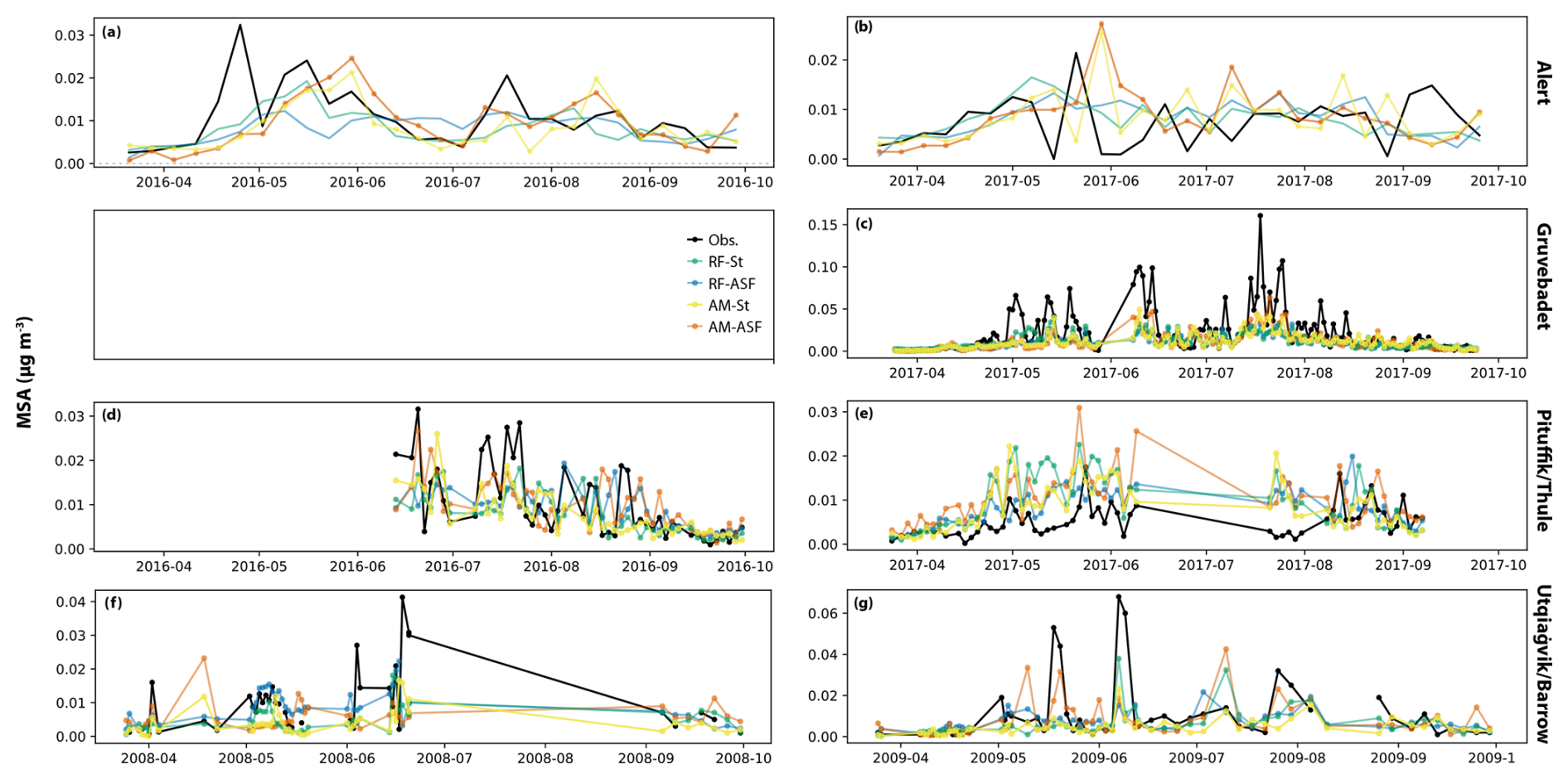
Figure 5Observed and modeled time series of MSAp for the test dataset at all four stations: (a, b) Alert, (c) Gruvebadet, (d, e) Pituffik (Thule), and (f, g) Utqiaġvik (Barrow). St refers to a model trained and tested on the specified station, and ASF refers to all data from all four stations and tested only on the specified station. The observations are shown in black. Data from Gruvebadet during 2016 are not available.
3.4 Selected features
Features contributing significantly to the RF and AM model outputs for different backward time steps were selected from the Group A and A + B subsets for each model using the FSS (see Methods for more details). Group A included reliable features for prediction of MSAp, and Group B included features expected to be good predictors of MSAp, although less reliable. The right-hand panel in Fig. 6 summarizes which features are selected by which model over all time steps, for both the Group A and Group A + B subsets of variables, for every station, and for the two additional merged datasets AS and ASF. Generally, AM selects fewer features than RF over the four stations (Table 4). AM selects between two and eight variables for Group A and between three and six for Group A + B, whereas RF selects between 14 and 44 features for Group A (an exception being Pituffik (Thule), for which the models select five variables at most in Group A; see below) and between 14 and 17 features for Group A + B. This suggests that the variables in Group A + B can explain the MSA variance using fewer variables.
The differences in selected variable counts between RF and AM can likely be explained by the fact that RF has some difficulty distinguishing between features computed at various time steps backward for the same feature type, in comparison to AM. This is because each of the features computed for a given backward time step tends to correlate substantially (e.g., meteorological conditions are usually correlated to the previous days' conditions), which can make RF feature ranking inconsistent across the different decision trees. Therefore, each decision tree will likely only select one specific time step of a feature, if that feature group happens to be important for MSAp overall. Thus, by averaging over all trees, the different time steps of a given feature type are likely to be ranked similarly and the strength of the ranking score is averaged out. In contrast, AM is not an ensemble, and its variable selection operates sequentially; therefore if a backward time step for a given feature (among the five time steps) is already included and if the other four are strongly dependent and not adding additional information to the model, then they will likely not be selected. Therefore, the most relevant time step is selected consistently with AM, while RF selects different time steps of the same variable. Another contributing factor to the difference between the number of features selected by each model could be the sensitivity of the cutoff threshold (5 %) in the FSS procedure, which would disproportionately impact the ensemble RF model over AM. The prediction performance is similar for both models (Fig. 4); therefore we can compare the selected features for each model on an equal footing. The two models were also compared with features grouped for all five backward time steps (left-hand panel of Fig. 6), which shows that a similar number of features were chosen for RF and AM when the backward time steps were not considered separately. While the models disagree on the number and which backward time step is important for MSAp prediction, importantly, they do agree on which features are most important, indicating these models can learn the same underlying factors that drive MSAp levels.
The features selected by each model and station combination for Group A + B are listed in Table 4, where a common theme for the type of features selected emerges. Each model and station combination tends to select a source-related feature (related to either marine biogenic emissions, total DMS emitted or ChlA, or air mass contact with surface environments, time spent over open water, OPEN_WATER, residence time in the boundary layer, BL_RT), a chemical-processing-related feature (solar radiation (SSRD), OH, O3, specific humidity (Q), cloud liquid water content (LWC)), and a removal-related feature (large-scale rain rate, LSRR). For instance, AM for Gruvebadet selected four features, which are related to marine emissions of DMS (ChlA_1.2 and DMS_4.5), oxidation of DMS and its intermediates to MSA (OH_BL_0.1), and removal (LSRR_1.2). There are, however, exceptions to this tendency; notably a removal-related feature is mainly absent from the model–station combinations (Alert RF, Gruvebadet RF, Pituffik (Thule) RF/AM, and AS RF) and for Utqiaġvik (Barrow) AM and RF, a source-related features are absent.
Another important observation from the analysis of the selected features is that models trained on Group A + B tend to select much fewer meteorological features than models trained on only Group A. For example, specific humidity (Q) and temperature (T) are often selected if the smaller group, Group A, is being used but are almost never selected when using Group A + B. A possible explanation for this is that some features that are in Group B but not in Group A correlate with such meteorological variables, likely because they are driven by or co-vary with meteorological processes, e.g., solar radiation being a proxy for OH levels. This suggests that the smaller number of features selected from Group A + B (including oceanic biological, oxidant, and precipitation features, Tables 2 and 4) is better suited to capturing the variability in MSA compared to a larger number of mainly meteorological features selected from Group A. We separated the input features into two groups to examine how the data-driven models predict MSAp when only using reliable meteorological features and when additional chemical and oceanic related features were used as input. Comparing the evaluation metrics between models trained on Group A variables (Fig. S5) and Group A + B (Fig. 4), we can see there are no clear systematic differences between station–model combinations trained on different input data groups. Models trained only on reliable features (Group A) can perform similarly to models trained on all features (Group A + B); therefore modeling MSAp in the Arctic can likely be achieved only using meteorological features that act as proxies for chemical and oceanic processes without negatively compromising model performance.
3.4.1 Source-related features
For the source-related feature type, which is related to the marine emission of DMS either directly (DMS emission) or indirectly (ChlA or OPEN_WATER), RF and AM do not agree on the selection of DMS. RF never selects DMS, while AM selects it for all sites except Pituffik (Thule). A possible explanation for this is that ChlA acts as a proxy for the biological activity that drives seawater DMS production and emission (Mansour et al., 2020; Rinaldi et al., 2013). Indeed, ChlA is chosen by RF for Gruvebadet, AS, and ASF. Importantly, AM never selects the 0–1 d back version of DMS, and the earliest time step selected is 2–3 d back for ASF as well as the 3–4 d back version for Utqiaġvik (Barrow) and Pituffik (Thule). Conversely, both AM and RF select early time steps of ChlA, with the latest being 2–3 d back. This could be due to differences in the nature of the data source, with ChlA being a satellite product vs. DMS emissions being parameterized based on wind speed, sea surface temperature, and seawater DMS climatologies (see Methods). The presence of clouds, which obscure the satellite view, could also affect the time steps selected for ChlA. Even though the ChlA dataset used should minimize the effect of clouds, their influence is still present, while the DMS climatology is unaffected by their presence. Missing ChlA was imputed, and this could also affect the results shown here. The other source-related feature selected is the time air masses spent within the boundary layer and over open water (sea ice < 20 %, OPEN_WATER), with both models selecting this feature for different stations and days backward. RF selected OPEN_WATER_3.4 for Alert, while AM selected the 0–1 and 4–5 d back versions for ASF and Pituffik (Thule), respectively (Table 4). Overall, while there is some disagreement between RF and AM on which source-related features are selected, both models can learn that a certain time lag seems necessary for air mass contact with biologically active marine environments to predict MSAp well, which indicates the results from the models are physically plausible.
3.4.2 Chemical-processing-related features
For the chemical-processing-related feature type, which is related to the photo-chemical oxidation of DMS and its intermediates into MSA either in the gas or aqueous phase, surface shortwave radiation downwards (SSRD) is commonly selected by all models when training models on Group A features only. When training models on Group A + B features, RF also always selects at least one version of SSRD, while AM only selects SSRD for Alert and Pituffik (Thule). Thus, SSRD generally appears to be a strong predictor of MSAp, which is expected given the need for solar radiation in the generation of photochemical oxidants required for MSAp production, in both the gas and aqueous phases (Jiang et al., 2023; Wollesen de Jonge et al., 2021). AM almost exclusively selects the 0–1 time step of SSRD, which hints at the near-immediacy of a causal relation between solar radiation and MSAp generation, likely through the production of OH radicals and other photochemical oxidants (e.g., BrO and aqueous-phase O3). Gas-phase OH radical mixing ratios (for either the boundary layer or the free troposphere) are directly selected by both models at all sites except Utqiaġvik (Barrow). When AM selects OH, it is mainly the 0–1 or 1–2 d back time step, and either the BL or FT versions are selected depending on the station. This indicates that OH mixing ratios are making the largest impact on the model both aloft and close to the surface in the preceding 2 d before measurement. The lifetime of DMS is estimated to be on the order of days in the Arctic (Breider et al., 2010; Lundén et al., 2007), although the lifetime of the intermediate compounds dimethylsulfoxide (DMSO) and methanesulfinic acid (MSIA) is both less than 1 d (Hoffmann et al., 2016; Zhu et al., 2003). This indicates that the detected MSAp could be formed in close proximity to the measurement stations when sufficient solar radiation and photochemical oxidants become readily available (Collins et al., 2017; Jiang et al., 2023). Interestingly, neither model selected any version of OH for Utqiaġvik (Barrow) (Table 4); instead specific humidity (Q) and cloud liquid water content (LWC) were selected, and Utqiaġvik (Barrow) is the only station where gas-phase O3 was selected (RF). It should be noted that gas-phase OH and O3 will dissolve into the aqueous phase, thus also affecting aqueous-phase reactions as well. The selection of SSRD and OH at Alert, Gruvebadet, and Pituffik (Thule), as well as the selection of LWC and Q at Utqiaġvik (Barrow), hints at differences between the chemical processing between these stations during months of peak concentration. Utqiaġvik (Barrow), with its MSAp seasonal cycle peaking in late summer (Fig. 2b), is located in the Pacific sector of the Arctic, while the other stations, with MSAp peaking in early summer, are located in the Atlantic sector (Fig. 2a). The selection of different chemical-processing-related features for Utqiaġvik (Barrow) and the geographic differences in relation to biologically active waters, sea ice, and ocean dynamics could explain the different seasonal cycle observed at Utqiaġvik (Barrow) compared to the other stations. This analysis cannot quantitatively determine the relative importance of gas- vs. aqueous-phase oxidation; previous research indicates that both are likely contributing to Arctic MSAp production (Chen et al., 2023; Kecorius et al., 2023; Pernov et al., 2024b; Shen et al., 2022). This study suggests that depending on the time of year and geographic location, different chemical processing mechanisms might be relatively more important. While there is disagreement between the most frequently selected time step for DMS (4–5 d back) and ChlA (2–3 d back), the selected time steps for these features still mainly occur temporally before SSRD or OH when these features are selected together, indicating that our data-driven models can learn the temporal dependencies of the source- and chemical-processing-related feature types affecting MSAp.
3.4.3 Removal-related features
The main removal pathway for MSAp is wet deposition, and LSRR (large-scale rain rate, Table 4) was selected by most model–station combinations to represent the removal of aerosols. Interestingly, the only other removal-related feature (time air masses experienced precipitation, PRECIP, including rain, snow, and a mix of both) is never selected by any model–station combination (Fig. 6 and Table 4). Particulate mass quickly decreases with initial increases in accumulated precipitation during air mass transport and levels off with larger amounts of precipitation (Isokääntä et al., 2022; Tunved et al., 2013). The PRECIP feature only estimates the time air masses experienced precipitation and does not account for the intensity. This could explain the selection of LSRR over PRECIP and suggests that the time air masses experienced precipitation (regardless of type – rain, snow, or mix) is less important compared to the intensity of precipitation (estimated by LSRR). The LSRR time steps selected, however, showed no consistent pattern, with different daily intervals being selected for different model–station combinations (Table 4). Precipitation can have dual effects on MSAp, where precipitation closer to the station can act to remove aerosols resulting in lower MSAp, while precipitation further back along the trajectory can create conditions conducive for secondary aerosol formation (for which MSA is an important component) (Khadir et al., 2023; Tunved et al., 2013; Xavier et al., 2022). These dual effects could complicate the consistent selection of time steps for LSRR. The below-cloud scavenging coefficient of aerosol particles reaches a minimum in the accumulation mode (Andronache, 2003), which is where MSAp mainly resides (Kerminen et al., 1997); these aspects could also complicate the selection of removal-related features. Overall, this shows that the data-driven models can discern removal mechanisms for MSAp, although it does not specify when precipitation is important and suggests that precipitation intensity (LSRR) is relatively more important than the total time air masses experienced precipitation (PRECIP).
3.4.4 Physical-meteorology-related features
Other feature types born out of the FSS procedure include physical-meteorology-related features (e.g., boundary layer height (BLH) and wind speed (WS)), which can affect the sources, oxidation, and removal of precursors and MSAp depending on the prevailing environmental conditions. High wind speed can bring nutrients to the ocean surface, thus stimulating marine biological activity and enhancing the ocean–atmosphere flux of DMS (Huebert et al., 2010; Park et al., 2013), but can also increase the oceanic mixed layer depth, thus acting to delay spring phytoplankton blooms (Henson et al., 2009). Dry deposition of trace gases and aerosol particles is largely determined by turbulence, which is driven by wind speed (Farmer et al., 2021); thus higher wind speeds can enhance dry deposition velocities (Mariraj Mohan, 2016), enhancing the removal of aerosols. High boundary layer heights can promote or diminish MSA burdens: high BLHs can dilute DMS in the lower atmosphere, thus enhancing emissions but also diluting the oxidants and lowering the efficacy of MSAp production. High BLHs close to the station can also dilute MSAp concentrations. While the models mainly selected source-, chemical-processing-, and removal-related features, this shows that specific meteorological conditions can also affect MSAp variability.
3.4.5 Vertical origins
Certain datasets (CAMS and ERA5 on model levels; see Methods) were vertically resolved, which allowed for analysis of environmental conditions near the surface (or boundary layer, BL) and aloft (or free troposphere, FT). Similar to the different days back time steps of a feature, AM selects only the most pertinent feature that contributes the most to the model output, as our variable selection procedure for AM performs this process sequentially by design, while RF trees select several different time steps, and vertical origins for each feature from a random subset thus might not be a globally optimal choice. This highlights the complementary nature of these two models for the feature-engineered input data – AM selects fewer features but specifically the ones that make the largest contribution to the model output, while RF can broadly indicate the important features regardless of time step or vertical origins. While this analysis cannot quantify the relative importance of BL or FT processes to MSA production, it is worth noting that AM for Alert and Pituffik (Thule) (two stations located above the sea surface, Table 1) selected OH_FT_1.2, while Gruvebadet, Utqiaġvik (Barrow), AS, and ASF selected more BL than FT features (Table 4), and OH_BL was selected at these stations except for Utqiaġvik (Barrow) where Q_BL_0.1 and LWC_BL_2.3 were selected. This suggests that the two stations located at elevation are more influenced by FT processes than the stations located close to the surface and the pan-Arctic merged datasets (AS and ASF).
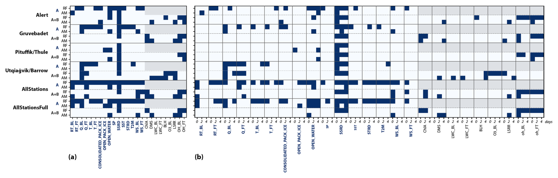
Figure 6Overview of features selected by the RF and AM based on Group A and Group B, by station. The left panel shows selected features grouped over the 0–5 d prior to each MSAp measurement, and the right panel shows the features grouped for 0–1 (0), 2–3 (2), and 4–5 (4) d before each MSAp measurement. Features in Group A have their name in boldface and blue type, while the additional features that are only in Group B are in regular black typeface. The grey shaded area indicates that Group B features cannot be chosen in these model runs. St refers to a model trained and tested on the specified station, AS refers to a subset of the data with an equal number of observations from each station, and ASF refers to all data from all four stations and tested only on the specified station. Feature abbreviations are defined in Table 2. Only features selected at least once by a model–station combination are presented in this figure (i.e., if a feature is not included in the figure, then it was not selected).
Table 4Features selected by the different models using the Group A + B set of variables. N is the number of selected features. The chosen features are listed in order of importance for the model. Feature names are in the following format: ABBREVIATION_DAYS.BACK with the ABBREVIATION for each feature taken from Table 2 and DAYS.BACK the daily interval backward in time preceding the measurement with the interval separated by a period. Whether the feature represents the boundary layer (BL) or free troposphere (FT) is also indicated; e.g., OH_BL_2.3 refers to the OH radical mixing ratio in the boundary layer 2–3 d before MSAp measurement.
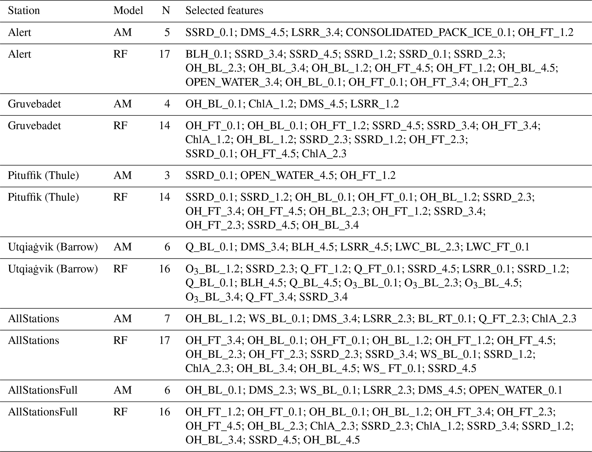
3.5 Contribution of selected features to model output (partial effects) for Alert and Utqiaġvik (Barrow)
We investigated the relationships between the selected features and the AM output of MSAp, which produces estimated partial effects (representing the contribution of a feature to the model output after accounting for all other features; see Methods for more details) for every selected feature for every station and the merged datasets (AS and ASF). Figures 7 and 8 present the partial effects (as the solid red line) for the selected features at Alert and Utqiaġvik (Barrow), respectively, and the partial effects for Gruvebadet, Pituffik (Thule), AS, and ASF are displayed in Figs. S8–11, respectively. We present the partial effects for Alert and Utqiaġvik (Barrow) as they are good examples of the relative importance of the two chemical processing methods observed in the study, gas- and aqueous-phase oxidation, respectively. The partial effects for each feature are discussed in order of importance from the feature selection process (Table 4). It should be noted that due to the different aggregation methods (sum or mean, Table 1) over the different temporal resolutions at each station (Table 2), the magnitude and units of certain features are not comparable between stations; therefore for display purposes only the summed features were divided by the average number of input data contributing to the summed feature. In this manner, the partial effects plots are comparable between stations. For each subpanel, a scatter plot of the input variables and the corresponding model output of MSAp is also included. The partial effects should not be interpreted as a fitted value of this scatter plot. The scatter plot was included to show the data distribution and the low signal-to-noise ratio visible in the data: the observations have quite a large spread relative to the magnitude of the solid red curves, representing the partial effects. It should also be noted that spline functions, like the B splines used in the AM model (see Methods), are generally sensitive near the edges of the observed domain space if they contain few data points. Therefore, caution is urged when interpreting the partial effects if the data are highly skewed or if a few data points are contained at the edges of the domain space.
3.5.1 Alert
AM selected the following features at Alert, which are discussed in order of importance: SSRD_0.1, DMS_4.5, LSRR_3.4, CONSOLIDATED_PACK_ICE_0.1, and OH_FT_1.2, as well as the interactions between DMS_4.5 and SSRD_0.1 (Fig. 7).
SSRD_0.1, a chemical-processing-related feature, makes a non-linear contribution to the model output of MSAp, with the maximum impact on model output in a certain range of values as well as low and high values of SSRD making similar contributions to model output (Fig. 7a). This indicates that there is a certain activation threshold of SSRD_0.1 required before this variable begins to increase MSAp in the model output, which is likely connected to the production of photochemical oxidants (Barnes et al., 2006a; Song et al., 2022). Increasing SSRD above this threshold reduces the model output, which could be due to photolysis of intermediate products during DMS oxidation or the continued oxidation of MSA to sulfate (Chen et al., 2018).
DMS emissions during 4–5 d prior to observation, a source-related feature, shows a linearly positive relationship to model output of MSAp, as expected (Fig. 7b). However, a slight change in the slope of this relationship is observed, indicating that the model output of MSAp is more sensitive to DMS emissions at lower values (with MSAp production likely being in a DMS-limited regime) and less sensitive at higher values (with MSAp production likely not limited by DMS availability but by other environmental conditions such as oxidants, Barnes et al., 2006a).
LSRR, a removal-related feature, makes a linearly, negative contribution to the model output of MSAp, indicating that precipitation acts to reduce the model output of MSAp (Fig. 7c), as expected (Isokääntä et al., 2022; Tunved et al., 2013). While this result is unsurprising, it adds validity to the model results by highlighting how they are physically interpretable.
The partial effect of CONSOLIDATED_PACK_ICE, here treated as an indirect source-related feature, shows a non-linear relationship to model output of MSAp (Fig. 7d), with a maximum (minimum) at ∼ 200 (∼ 400) s km−2, respectively. Alert, being the northernmost station (Table 1), is usually surrounded by consolidated pack ice (Kwok, 2018); hence the transport time over consolidated pack ice will usually be non-zero. The maximum at ∼ 200 s km−2 could indicate that air masses traversed biologically productive marginal ice zones before passing over consolidated pack ice and ultimately arriving at Alert (Sharma et al., 2012). The minimum of the partial effects at ∼ 400 s km−2 is likely related to air masses spending time over the central Arctic Ocean and that did not come into recent contact with any major DMS source regions.
OH_FT_1.2, a chemical-processing-related feature, shows a non-monotonic pattern, with a maximum of around ∼ 1.5 × 10⁻⁵ ppbv and a minimum at ∼ 4 × 10⁻⁵ ppbv (Fig. 7e). The maximum and minimum could indicate that a certain level of OH in the FT acts to produce MSAp, and increasing OH above this level in the FT tends to decrease the model output of MSAp. A possible explanation could be the oxidation of intermediate compounds, DMSO and MSIA, to produce MSAp, and the continued oxidation of MSA to sulfate to diminish MSAp (Hoffmann et al., 2016). It should be noted that gas-phase OH will dissolve into the aqueous phase; therefore these reactions could both occur in either phase.
Interactions between input features were also explored by multiplying the values of two input features together. Of the combinations tested for all features and stations, only the interactions between DMS_4.5 and SSRD_0.1 at Alert were retained (using the FSS with a 5 % MSE reduction threshold; see Sect. 2.6.2). A contour plot of the model output of MSAp for different values of DMS_4.5 and SSRD_0.1 is shown in Fig. 7f. The results overall suggest that model output of MSAp is more sensitive to DMS_4.5 compared to SSRD_0.1, as indicated by the higher variability of MSAp model output over the range of DMS_4.5 at a fixed value of SSRD_0.1. This is especially evident for values of SSRD_0.1 above 400 W m−2, with a ridge of the maximum model output of MSAp for values of SSRD_0.1 around ∼ 700 W m−2 (Fig. 7f). Taken together, this could indicate that at Alert, MSAp production is likely limited by DMS emissions and not necessarily by the availability of solar radiation (and therefore photochemical oxidants).
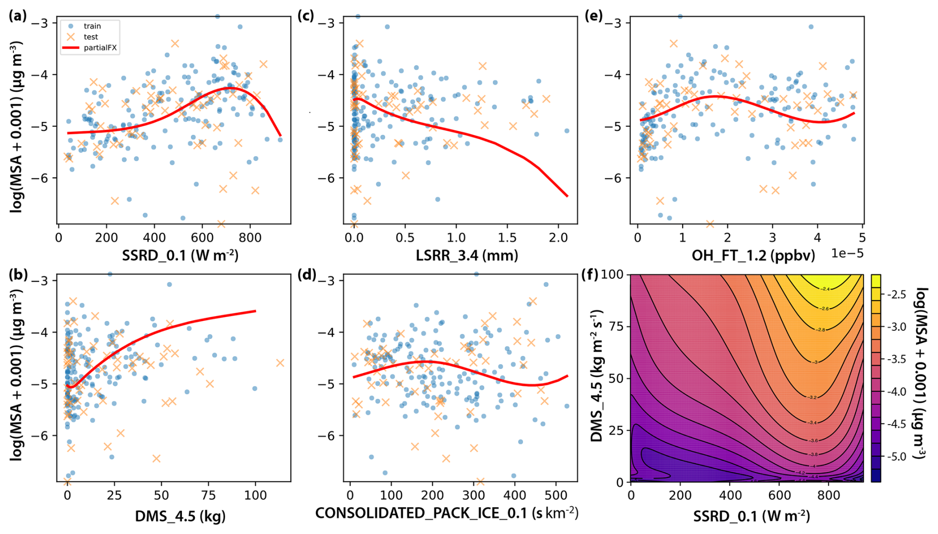
Figure 7AM-St partial effects for the selected features at Alert. (a) SSRD_0.1, (b) DMS_4.5, (c) LSRR_3.4, (d) CONSOLIDATED_PACK_ICE_0.1, (e) OH_FT_1.2, and (f) DMS_4.5 and SSRD_0.1. For all panels except the bottom-right one, the solid red line is the partial effect for a different feature, blue points are the training observations, and orange crosses are the test data. The contour plot in the bottom-right panel shows the interaction effect between SSRD_0.1 and DMS_4.5, where the joint partial effect is represented by the color gradient. Feature abbreviations are defined in Table 2. St refers to models trained and tested on the specified station. Features aggregated as sums over filter time windows (see Table 2) are rescaled here by the average number of 3-hourly samples in each summation to help compare partial effects between stations.
3.5.2 Utqiaġvik (Barrow)
For Utqiaġvik (Barrow), AM selected the following features: Q_BL_0.1, DMS_3.4, BLH_4.5, LSRR_4.5, LWC_BL_2.3, and LWC_FT_0.1.
Specific humidity is the mass of water vapor per mass of moist air and here is used as a proxy of aqueous-phase processing of DMS and its intermediates. For Q_BL_0.1, which represents the specific humidity in the boundary 0–1 d prior to measurement, the lower end of the feature range (< ∼ 0.0025 kg kg−1) shows a small local maximum at ∼ 0.00125 kg kg−1. At the upper end, a linear, positive relationship between Q_BL_0.1 and the model output of MSAp is observed (Fig. 8a). This indicates that at lower values of Q_BL_0.1, the model output is showing a slight increase in MSAp and little variation with low values Q_BL_0.1 levels, and at higher values of Q_BL_0.1 the model output of MSAp responds linearly. This relationship hints that at low values of Q_BL, particles are not deliquesced yet and gas-phase oxidation could be more important, while at higher values of Q_BL, sufficient aerosol liquid water is present for aqueous-phase processes to become dominant. Another explanation for this relationship could be that moist air masses arrived from within the boundary layer and from marine regions, which would carry a higher signal of moisture uptake, although no air mass history features indicating transport from marine regions (e.g., DMS, ChlA, OPEN_WATER, RT_BL) were selected for Utqiaġvik (Barrow), suggesting this is improbable.
The partial effects for DMS_3.4 display a U-shaped relationship for values < ∼ 200 kg and afterward increase linearly (Fig. 8b). The partial effects start to decrease at high values of DMS_3.4, although the few data points in the region add uncertainty to this slope change. The majority of the data for DMS_3.4 are skewed towards lower values, which likely contributes to the U-shaped partial effects below ∼ 200 kg. Overall, the model output of MSAp increases with increasing DMS, again showing physically plausible results.
The BLH 4–5 d prior to observation shows an overall positive, linear relationship with the model output of MSAp, although with some complex structure present (Fig. 8c). In the Arctic, and especially over sea ice, the BLH is largely controlled by wind-shear-induced turbulence and cloud top radiative cooling (Nilsson, 1996; Overland, 1985; Tjernström et al., 2015). Recently, a gridded dataset of in situ-produced biogenic MSA (generated using machine learning) was published (Mansour et al., 2024) for the North Atlantic. An inverse relationship between BLH and in situ MSA was found, indicating that higher BLHs dilute the concentrations of MSA (Mansour et al., 2024). A machine learning study on the drivers of aerosol chemical composition from Svalbard indicated an inverse relationship between BLH and biogenic-type aerosols (Song et al., 2022). These studies indicate that lower BLHs act to increase the concentration of MSA, while higher BLHs dilute MSA in the lower troposphere. Our recent study analyzing the environmental drivers of MSA from a geographic perspective revealed that the relationship between MSA and BLH is complex and displays different patterns in different months (Pernov et al., 2024b), with high values of BLH tending to increase the model output of MSA in all months but low BLHs also increasing modeled MSA during June and July. Our recent study and this work indicate that higher BLHs act to increase the modeled output of MSAp, which could be due to higher wind speeds (and thus higher BLHs) diluting atmospheric DMS levels and therefore increasing the ocean–air flux of DMS. This also highlights the differences of considering air mass history when analyzing the relationships between aerosols and environmental drivers as opposed to considering only local, in situ explanatory variables.
The partial effects for LSRR_4.5 show a somewhat unexpected relationship, with a maximum at ∼ 1 mm and a linearly, negative relationship afterward (Fig. 8d). The minimum at > ∼ 4 mm is likely highly uncertain due to the low number of data points at the end of the feature domain space. A negative relationship is expected (and observed at other stations in this study and the literature) since precipitation acts to remove aerosols. The maximum of the LSRR partial effects at a non-zero value could be related to enhanced cloudiness and thus enhanced aqueous-phase processes although unlikely since AM selected the version of this feature 4–5 d back. Another possible explanation could be that low values of precipitation 4–5 d prior to measurement act to remove particles containing a high fraction of (possibly anthropogenic) sulfate (which are acidic and hygroscopic). Depending on the acidity of the remaining aerosols, this would create conditions that would favor the selective condensation of gas-phase MSA or diminish the evaporation of aqueous-phase produced MSA in less acidic particles since MSA has been shown to selectively condense on alkaline particles (Dada et al., 2022; Yan et al., 2020). The exact cause of the maximum LSRR_4.5 partial effect remains to be seen at this time and requires further investigation.
LWC_BL_2.3 (defined as the boundary layer cloud liquid water content 2–3 d prior to measurement) is the amount of cloud liquid water and thus an excellent proxy for aqueous-phase processing. The partial effects for LWC_BL_2.3 display two local maxima: one at ∼ 0.5 × 10⁻⁵ and another at ∼ 4 kg kg−1 (Fig. 8e) albeit with an overall linearly, positive relationship with the model output of MSAp. The decrease in the partial effects after ∼ 4 kg kg−1 carries added uncertainty due to the few data points but could possibly suggest the effect of precipitation at high values of LWC, thus acting to remove MSA. These two local maxima of LWC_BL_2.3 could indicate that gas-phase oxidation and aqueous-phase oxidation are the dominant mechanisms at lower and higher values of LWC_BL_2.3, respectively. If so, then the overall linearly, positive relationship for LWC_BL_2.3 and model output of MSAp could also indicate that aqueous-phase oxidation produces relatively greater amounts of MSAp compared to gas-phase oxidation, which is in line with the theoretical understanding (Chen et al., 2018; Hoffmann et al., 2016).
The amount of cloud liquid water in the free troposphere 0–1 d prior to measurement (LWC_FT_0.1) shows a similar relationship to model output of MSAp as does LWC_BL_2.3, with two local maxima, an overall positive relationship and a decrease in model output after the second local maxima (Fig. 8f). Noticeable exceptions include the overall response of model output of MSAp being less sensitive to increases in LWC_FT_0.1 compared to LWC_BL_2.3 and the decrease in model output after the second local maxima being more substantial. This relationship likely points towards gas- and aqueous-phase oxidation occurring at differing levels of LWC but also that the model output of MSAp is less sensitive to LWC in the FT than in the boundary layer and that high values of LWC in the FT more strongly remove aerosols than in the BL.
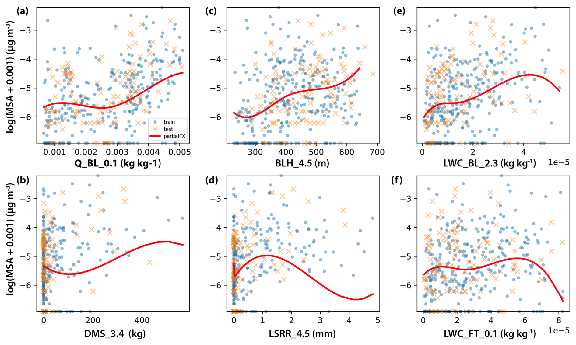
Figure 8AM-St partial effects for the selected features at Utqiaġvik (Barrow). (a) Q_BL_0.1, (b) DMS_3.4, (c) BLH_4.5, (d) LSRR_4.5, (e) LWC_BL_2.3, and (f) LWC_FT_0.1. The solid red line is the partial effect for a different feature in each panel, the blue points are the training observations, and the orange crosses are the test data. Feature abbreviations are defined in Table 2. St refers to models trained and tested on the specified station. Features aggregated as sums over filter time windows (see Table 2) are rescaled here by the average number of 3-hourly time steps to help compare partial effects between stations.
3.5.3 Summary of Gruvebadet, Pituffik (Thule), AS, and ASF
For Gruvebadet, AS, and ASF, a source-, chemical-processing-, and removal-related feature type were selected for AM, except for a removal-related feature being selected at Pituffik (Thule). The partial effects of the selected features for AM are discussed in detail in Sect. 3 of the Supplement. The chemical-processing-related feature type was usually OH for Alert, Gruvebadet, Pituffik (Thule), and ASF, while for Utqiaġvik (Barrow), Q and LWC were selected (Table 4), and interestingly the removal-related feature type (LSRR) showed a maximum at a non-zero value (Fig. 8d). The partial effects of Q and LWC show the presence of two local maxima and an overall positive relationship to model output of MSAp, suggesting that the dual effects of gas- and aqueous-phase chemical processing can be detected. Our previous study showed the importance of both gas- and aqueous-phase oxidation for the geospatial modeling of pan-Arctic MSA, with shortwave surface radiation (SSRD in this study), temperature (T2M), longwave surface radiation (STRD), and low cloud cover (LCC) being the top four important features. Interestingly, neither T2M, STRD, nor LCC was selected for any station–model combination (Table 4). It should be noted that Pernov et al. (2024b) utilized a different feature engineering procedure to account for air mass transport patterns, a different data-driven model (gradient boosted trees vs. RF/AM in this study), and different explainability methods (SHAP (Lundberg and Lee, 2017) vs. partial effects in this study) and focused on geospatial source regions from a pan-Arctic perspective and not time series of time-resolved air mass history features at individual stations; therefore a direct comparison is complicated by these facets. However, for the AS partial effects, the dual mechanisms of gas- and aqueous-phase oxidation are observed (both OH_BL_1.2 and Q_FT_2.3 were selected), indicating that modeling a merged pan-Arctic dataset can detect these dual processes are occurring, similar to our previous research. The ASF features selected by AM and RF did not include an aqueous-phase related oxidation feature (Table 4), which could be due to Gruvebadet contributing the greatest number of samples to the ASF-merged dataset; thus features selected at this station could dominate the selected features for ASF. Overall, the selected features and their partial effects for the individual stations and merged datasets show that our data-driven model produces physically realistic and interpretable results.
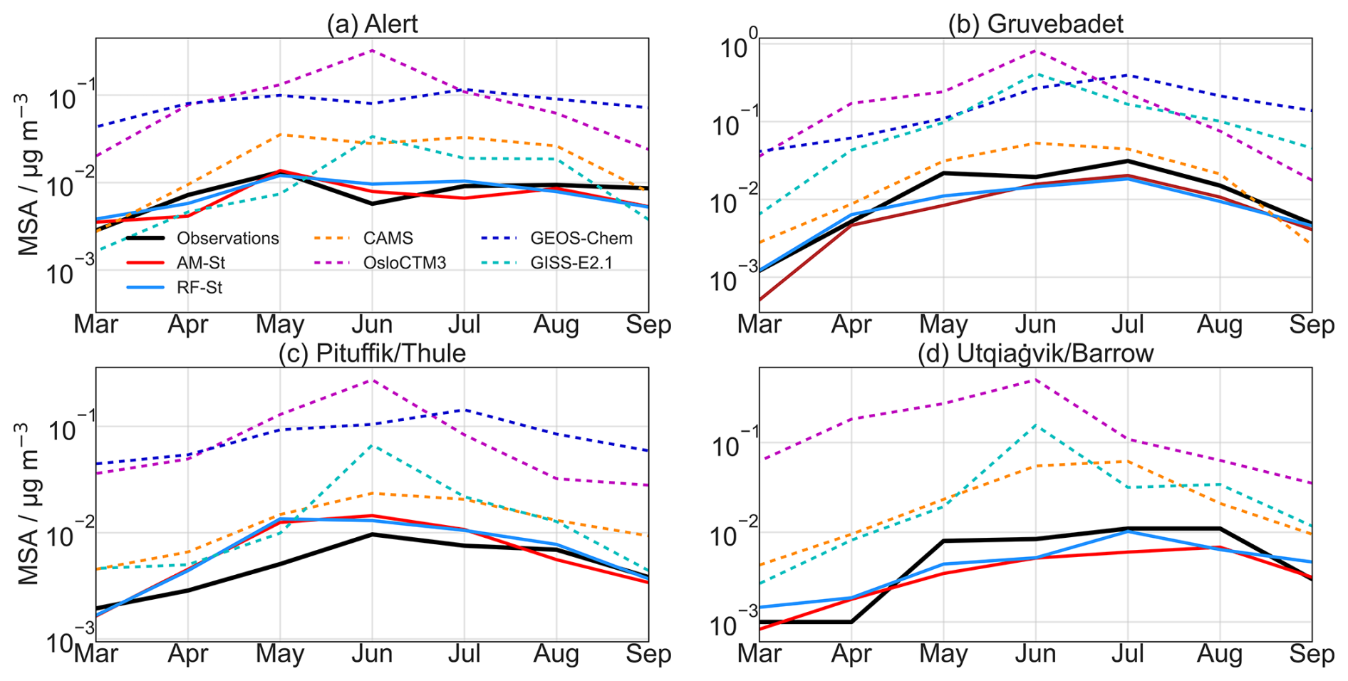
Figure 9Comparison of seasonal cycles for observations, St data-driven model, and numerical models. (a) Alert (b) Gruvebadet, (c) Pituffik (Thule), and (d) Utqiaġvik (Barrow). Monthly medians for observations (solid black), data-driven model (AM-St in solid red and RF-St in solid light blue), CAMS (dashed orange), GEOS-Chem (dashed dark blue), GISS-E2.1 (dashed cyan), and OsloCTM3 (dashed magenta). Only data for the tests were included in this analysis for a fair comparison; see Table 3 for dates. St refers to models trained and tested on the specified station. The evaluation metrics for each data-driven and numerical model against in situ observations are given in Fig. 10.
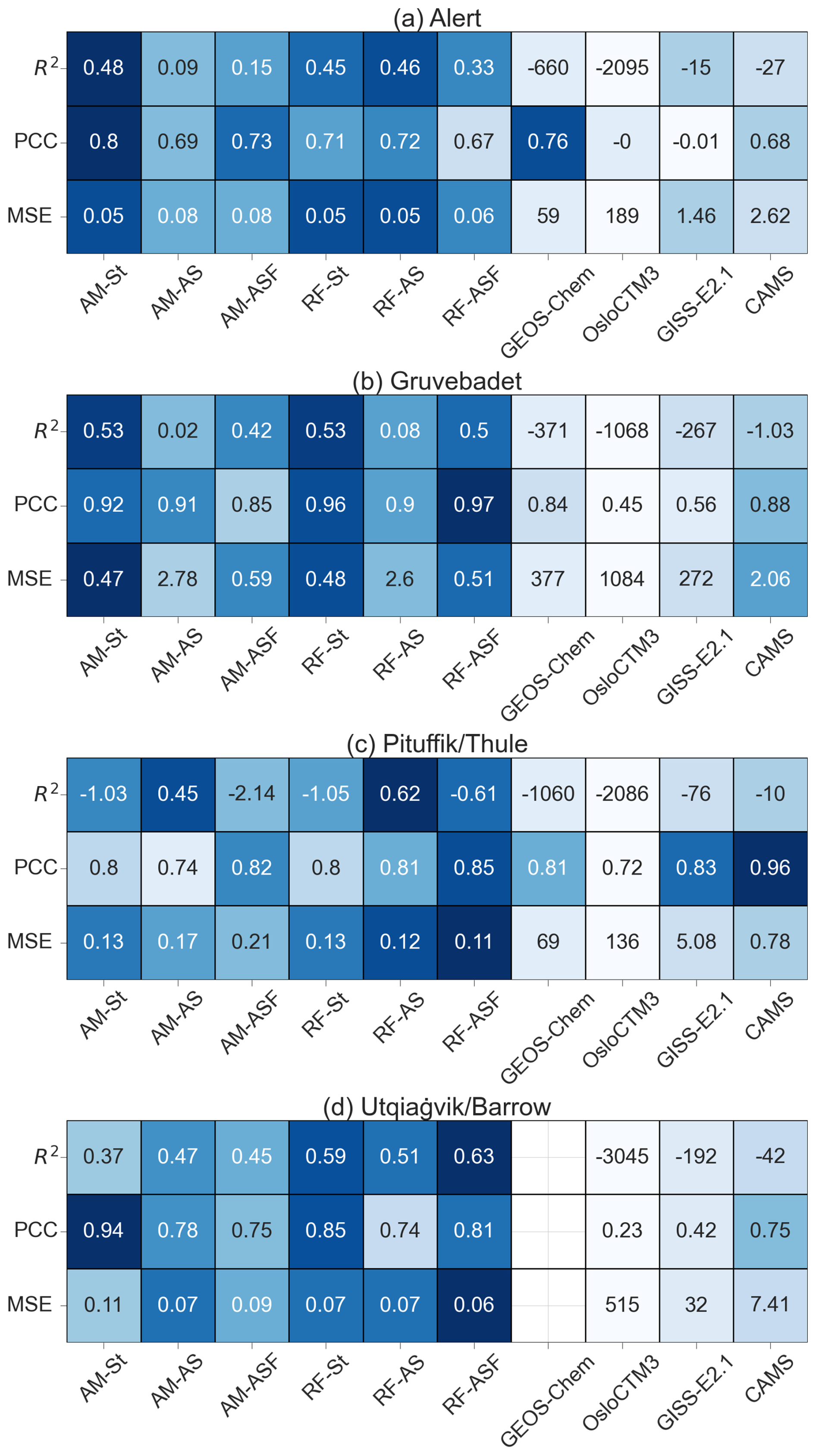
Figure 10Prediction performance for the data-driven and numerical models on the test set for the four stations for the random forest (RF) and additive model (AM). (a) Alert (b) Gruvebadet, (c) Pituffik (Thule), and (d) Utqiaġvik (Barrow). In each panel, R2 is shown in the top sub-panel, the Pearson correlation coefficient (PCC) in the middle sub-panel, and the mean squared error (MSE) at the bottom. St refers to a model trained and tested on the specified station, AS refers to a subset of the data with an equal number of observations from each station, and ASF refers to all data from all four stations and tested only on the specified station. MSE is multiplied by 104 to display three significant digits. The color scale indicates performance, where the darkest blue signifies the best performance (lowest MSE, highest R2, and highest PCC within each row). The MSE, R2, and PCC values are calculated according to Eqs. (1), (2), and (3), respectively.
The Arctic is undergoing drastic environmental changes, inducing alterations in the natural aerosol population, which in turn affect the Arctic climate. Due to complex feedback mechanisms in the Arctic climate system, numerical modeling is vital for understanding and predicting upcoming climate change and the role of natural aerosols therein. However, numerical models are deeply challenged in representing natural aerosols across the Arctic. Data-driven modeling can be a faster and less computationally intensive alternative for simulating Arctic aerosol processes, which can also identify important processes and variables to inform improvement efforts for numerical models. Therefore, we developed an alternative data-driven modeling approach for modeling Arctic MSAp using long-term in situ observations of MSAp from four High Arctic stations.
We developed an AM for the task of predicting MSAp observations. This tailored model allowed for more interpretable estimated relations (partial effects) in a more parsimonious format than the RF model, which served as a baseline, and this with both data-driven models achieves similar out-of-sample prediction performance. We incorporated feature selection procedures into both data-driven models, which selected similar features when not considering the temporal dimension (time step) of the features. However, RF selected more features compared to AM, when considering the time step, which could be attributed to the importance of different time steps being averaged out over the ensemble of decision trees in RF versus AM, which only selected the most important time step for each feature. We utilized two groups of features for data-driven modeling: one with only reliable features and one with all features related to MSA production regardless of data source and degree of reliability. When modeling using only reliable features (which were mainly meteorological), they can act as a proxy for unreliable features (e.g., solar radiation (SSRD) acting as a proxy for OH radical mixing ratios), although no systematic change in model performance was detected when including all features. Indicating that a similar model performance can be achieved by only using meteorological features but incorporating source-, chemical-processing-, and removal-related features (albeit with added feature uncertainty) resulted in fewer features being selected.
We show that existing numerical models struggle to accurately simulate MSAp in terms of the magnitude, seasonality, and peak months of concentrations, which can have consequences for accurate estimations of the surface energy budget and climate projections given the role of MSAp in the climate system (Fung et al., 2022; Mahmood et al., 2019). Our data-driven models outperform current numerical models for reproducing observations of MSAp, which is especially evident for the seasonal cycle. While data-driven models trained on merged datasets (AS and ASF) already outperform numerical models, the accuracy achieved by training on individual stations (St), is even higher (Fig. 4). A comparison of the seasonal cycle from numerical vs. data-driven models for only the test set years (thus a direct comparison of the same periods) is shown in Fig. 9, and evaluation metrics are shown in Fig. 10. Based on the correlation of monthly medians for the test set for each station, both the additive model (AM) and random forest (RF) can generally reproduce the seasonal cycle of MSAp, with greater accuracy than the numerical models based on the evaluation metrics used (Figs. 9, 10, S12, and S13), although there are few exceptions depending on station, dataset, and numerical model.
Both models consistently selected features that were related to the source of MSA precursors (emission of DMS and air mass contact with biologically productive marine areas), chemical processing of DMS (and its intermediates) to MSA (SSRD, OH, specific humidity (Q) and cloud liquid water content (LWC)), and removal of aerosols (large-scale rain rate, LSRR). The time steps selected by both models indicate that they can learn the correct timing of important processes related to MSA production; for instance when DMS and SSRD were selected together, the time steps for DMS emission always preceded those of SSRD. The features also included a vertical dimension (boundary layer vs. free troposphere). Results showed that the two stations located at elevated altitudes (Alert and Pituffik (Thule)) were likely more influenced by processes in the free troposphere than in the boundary layer, while the other stations (Gruvebadet and Utqiaġvik (Barrow)) and merged pan-Arctic datasets showed greater influences from the boundary layer. The relationships between the input features and the model output of MSAp were investigated through the partial effects produced by AM.
For Alert, Gruvebadet, Pituffik (Thule), and ASF, OH was the main chemical-processing-related feature selected, while for Utqiaġvik (Barrow), LWC and Q were selected, and for AS, both OH and Q were selected (Table 4). The selected features for AS suggest that the dual effects of gas- and aqueous-phase processing are occurring on a pan-Arctic scale. The selected features and their partial effects for individual stations reveal site-specific characteristics that are likely contributing to the differing MSAp seasonal cycles for stations located in different sectors of the Arctic.
While our methodology can outperform current numerical models, there is room for improvement. Our in situ observations were based on long-term datasets of low-temporal-resolution aerosol filter samples and were therefore limited in sample size. The input features were aggregated to the same temporal resolution as the collected filters, therefore fully capturing processes occurring on shorter timescales than the filter collection periods can be challenging. This is reflected in the ranking of data-driven model performance for the individual stations (Gruvebadet > Pituffik (Thule) > Utqiaġvik (Barrow) > Alert), which directly mirrors the decreasing temporal resolution of these stations (Table 1). Long-term, high-temporal-resolution MSAp measurements are essential for accurately capturing processes that are short-lived and highly variable. When sufficient long-term high-resolution data become available, leveraging the power of other data-driven approaches (e.g., neural networks) could be an option for advancing data-driven modeling of Arctic aerosols. However, when limited by the sample size, less complex tree-based models and statistical methods can often perform on par or better than neural networks (Grinsztajn et al., 2022). One option would be to combine data-driven modeling with physically constrained loss mechanisms, known as physics-informed neural networks (PINNs) (Cuomo et al., 2022). This avenue could help ensure the proper ingredients (precursors, oxidants, meteorology, etc.) are present at sufficient levels and with the correct temporal occurrence. The multi-input/output functionality of neural networks could also help elucidate the branching ratio of DMS oxidation mechanisms and the partitioning between gaseous and particulate phase MSA. However, satisfactory long-term, high-resolution, concurrent measurements of gas-phase DMS, gas-phase MSA, and particulate phase MSA need to become available at appropriate locations dispersed around the Arctic region, which remains a challenge both logistically and monetarily. Essential sources and sinks related to the burden of MSA, e.g., DMS emission and precipitation, while included in our model, are difficult to accurately represent using climatology-based parameterizations and reanalysis products, respectively, and improved estimations, through either an updated climatology (Hulswar et al., 2022) or data-driven estimations (Wang et al., 2020), could be incorporated in future data-driven model updates. Representation of specific oxidants (e.g., halogen radicals and dissolved oxidants) is missing from our input features due to a lack of adequate datasets. Incorporating accurate representations of these crucial species would help the data-driven models elucidate the relative importance of gas- versus aqueous-phase oxidation of DMS and specific oxidants. Another missing component from our feature list is aerosol chemical and physical properties (e.g., surface area, mixing state, hygroscopicity, and composition), which largely determines the reactive uptake of gaseous MSA (and its intermediates) onto preexisting aerosols (Dada et al., 2022; Yan et al., 2020). Acidic and effloresced aerosols are less likely to uptake gaseous MSA, while alkaline and deliquesced aerosols are more likely; including these parameters in future data-driven approaches could help resolve the equilibrium partitioning between gas and condensed phase MSA, thus representing another sink term for MSAp. One of the main shortcomings of the data-driven models is the inability to capture peak or minimum concentrations, which could be due to the low temporal resolution of the input target data into the models, inadequate representation of sources/sinks, the input data missing important features (such as dissolved oxidants or halogen species), processes occurring on timescales longer than the 5 d utilized in this study, or the daily interval between time steps being too coarse. Future data-driven modeling efforts could focus on capturing the drivers related to these extremes of the MSA distribution.
This data-driven modeling methodology using the time-resolved air mass history can be applied to other atmospheric constituent datasets at these Arctic stations for the study period, allowing researchers to investigate other natural aerosol components or precursor species (e.g., sea salt or dimethyl sulfide) in a consistent and time-efficient manner.
We recommend that numerical models be evaluated for the following processes that we identified as critical with our two data-driven model approaches: DMS emission, chemical processing, and removal.
-
Oceanic emission of DMS is the initial step for MSA formation, and AM identified DMS emission, OPEN_WATER, and ChlA as key features. The numerical models in this study all utilized climatologies of seawater DMS concentrations and parameterizations for estimating the DMS flux. Updating DMS emissions schemes using data-driven modeling can help improve estimates of MSA and sulfate as well as radiative forcing (Mansour et al., 2023; McNabb and Tortell, 2022; Regayre et al., 2020; Wang et al., 2020; Zhao et al., 2022). Current DMS emission parameterizations rely on seawater concentration, sea surface temperature, and wind speed (Johnson, 2010; Lana et al., 2011; Nightingale et al., 2000), although studies show real-world emissions are affected by atmospheric DMS levels, air temperature, pH, and nutrient availability (Hopkins et al., 2023; Kloster et al., 2007; Steiner et al., 2012; Sunda et al., 2007; Zhao et al., 2024; Zindler et al., 2014). Improved DMS emission inventories should be a focus of the modeling community going forward through either updated parameterizations or data-driven estimates (Joge et al., 2024a, b).
-
The data-driven models identified gas- and aqueous-phase oxidation to be affecting peak concentration months at different locations around the Arctic, namely OH, SSRD, LWC, and Q. Numerical models employ a plethora of chemical schemes for the oxidation of DMS and its intermediates, although shortcomings exist regarding aqueous phase oxidation, rate reaction coefficients, and oxidant concentrations (Bhatti et al., 2024; Cala et al., 2023; Chin et al., 1996; Fung et al., 2022; Hoffmann et al., 2021; Revell et al., 2019; Tashmim et al., 2024). This work and our previous work (Pernov et al., 2024b) point towards the dual effects of gas- and aqueous-phase oxidation both being key processes. Improvements to chemical processing schemes, especially aqueous-phase oxidation, as well as the inclusion of oxidants (halogens) and intermediates (DMSO, MSIA, and HPMTF) and their concentration levels, should be a priority of the modeling community going forward (Chen et al., 2018; Hoffmann et al., 2021; Jongebloed et al., 2024; Tashmim et al., 2024).
-
The removal of MSA through wet deposition (LSRR) was found to be a key feature identified via AM at all stations/datasets except for Pituffik (Thule) and Utqiaġvik (Barrow) (Table 4); however wet deposition is the key removal mechanism of MSA (Chen et al., 2018). Although dry deposition was not explicitly represented by our features, wind speed can be used as a proxy and was only selected by AM when considering the AS and ASF datasets and when their relationship with MSAp output was negative (Figs. 10 and 11). Numerical models could benefit from improvements in representations in wet deposition including aerosol activation, below- and in-cloud scavenging, and precipitation efficiency (Stier et al., 2024) as well as improvements in dry depositional processes.
Altogether, this study shows that (1) existing numerical models cannot yet simulate Arctic MSAp accurately, (2) data-driven models can outperform current numerical models although with modest performance, and (3) data-driven models can capture physically meaningful relationships between input features and MSA predictions quite well and reveal specific processes occurring at the different stations. While data-driven modeling can aid in simulating levels of natural Arctic aerosol and provide understanding of its drivers, it struggles with extrapolating beyond the distribution space of its training dataset; therefore numerical modeling is ultimately needed to predict the effects of a future climate on natural Arctic aerosol.
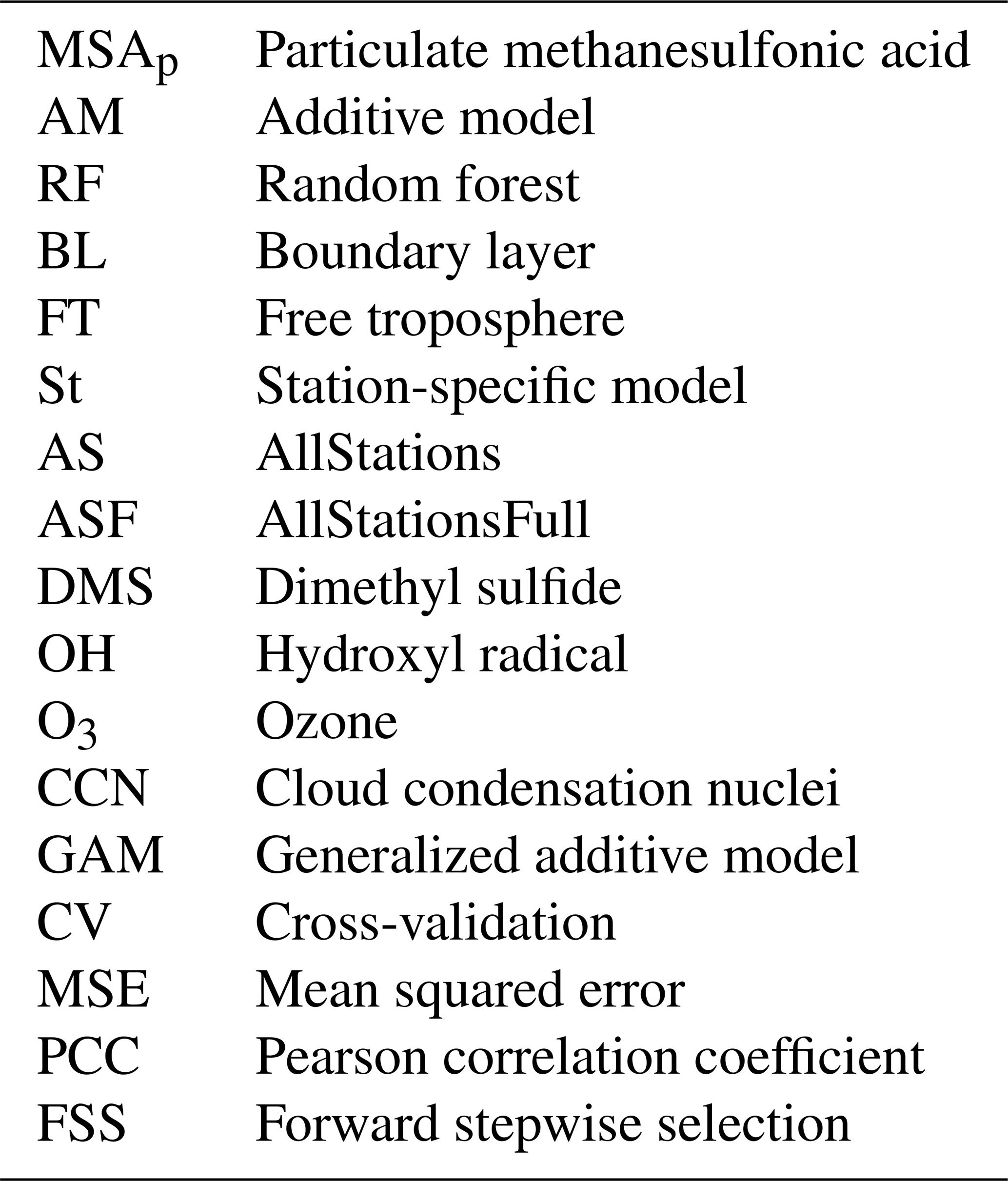
The underlying code for this study is available as a Renkulab project (https://gitlab.renkulab.io/arcticnap/msamodeling, Volpi et al., 2025) and by contacting the corresponding author Jakob Boyd Pernov (jakob.pernov@epfl.ch) or Michele Volpi (michele.volpi@sdsc.ethz.ch). Code for FLEXPART and Python packages (xESMF, cdsapi, and RF) is available online https://github.com/pangeo-data/xESMF, last access: 24 June 2025.
The datasets used and/or analyzed during the current study are available on reasonable request from the corresponding author Jakob Boyd Pernov (jakob.pernov@epfl.ch). ERA5 data are available from the CDS (https://cds.climate.copernicus.eu/#!/home, last access: 8 November 2022, Climate Data Store, 2025). CAMS data are available from the ADS (https://ads.atmosphere.copernicus.eu/cdsapp#!/home, last access: 8 November 2022, Atmosphere Data Store, 2025). DMS emissions are available at https://ads.atmosphere.copernicus.eu/cdsapp#!/dataset/cams-global-emission-inventories?tab=overview (last access: 15 September 2022, Copernicus Atmosphere Monitoring Service, 2020). In situ MSA is available online for Utqiaġvik (Barrow) (https://data.pmel.noaa.gov/pmel/erddap/tabledap/submicron.html, ERDDAP, 2025) and Alert (https://ebas.nilu.no/, EBAS home – ebas homepage, 2025), while Pituffik (Thule) and Gruvebadet are available upon request. FLEXPART is available upon reasonable request to Eliza Harris (eliza.harris@sdsc.ethz.ch). Chlorophyll a is available at https://www.globcolour.info/ (last access: 1 October 2022, GlobColour – Home, 2025).
The supplement related to this article is available online at https://doi.org/10.5194/acp-25-6497-2025-supplement.
JBP: conceptualization, methodology, software, validation, formal analysis, investigation, resources, data curation, writing (original draft), writing (review and editing), visualization, supervision, project administration. WHA: conceptualization, methodology, software, validation, formal analysis, investigation, resources, data curation, writing (original draft and review and editing), visualization, supervision, project administration. MV: conceptualization, methodology, software, validation, formal analysis, investigation, resources, data curation, writing (original draft and review and editing), visualization, supervision, project administration. EH: conceptualization, methodology, software, validation, formal analysis, investigation, resources, data curation, writing (original draft and review and editing), visualization, supervision, project administration. BH: conceptualization, methodology, software, validation, formal analysis, investigation, resources, data curation, writing (original draft and review and editing), visualization. RBS: software, validation, resources, data curation, writing (review and editing). SI: software, validation, resources, data curation, writing (review and editing). SH: software, methodology, software, writing (review and editing). UI: software, validation, resources, data curation, writing (review and editing). PKQ: methodology, validation, resources, data curation, writing (review and editing), funding acquisition. LMU: methodology, validation, resources, data curation, writing (review and editing), funding acquisition. JS: conceptualization, methodology, investigation, resources, writing (review and editing), funding acquisition, supervision, project administration.
At least one of the (co-)authors is a member of the editorial board of Atmospheric Chemistry and Physics. The peer-review process was guided by an independent editor, and the authors also have no other competing interests to declare.
Publisher’s note: Copernicus Publications remains neutral with regard to jurisdictional claims made in the text, published maps, institutional affiliations, or any other geographical representation in this paper. While Copernicus Publications makes every effort to include appropriate place names, the final responsibility lies with the authors.
This research was funded by the Swiss Data Science Center project C20-01 Arctic climate change: exploring the Natural Aerosol baseline for improved model Predictions (ArcticNAP). Julia Schmale holds the Ingvar Kamprad Chair for Extreme Environment Research sponsored by Ferring Pharmaceuticals. This project received funding from the Ingvar Kamprad Chair funded by Ferring Pharmaceuticals. This is a PMEL contribution 5669 and CICOES publication number 2024-1341 and was also funded by the U.S. National Science Foundation (2127733). Ulas Im acknowledges European Union's Horizon Europe project “CleanCloud” (grant agreement no. 101137639). We would like to thank Environment and Climate Change Canada, CCMR, CRD, Sangeeta Sharma, technicians (Joe Kovalik, Armand Gaudenzi, Dave Halpin, Dan Veber, Desiree Toom, and Alina Chivulescu), students, and operators at the Alert station, who assisted in the filter collection, processing, and laboratory analyses of methanesulfonic acid. The Department of National Defense and Canadian Armed Forces staff is acknowledged for providing support at the Canadian Forces Station Alert. We would also like to thank the technicians, support staff, students, and scientists, who helped obtain, analyze, and process the MSA measurements at Pituffik (Thule), Gruvebadet, and Utqiaġvik (Barrow). We would like to specifically thank Silvia Becagli and Rita Traversi from the University of Florence and the Institute of Polar Sciences at the National Research Council of Italy for providing in situ aerosol measurements from Gruvebadet and Pituffik (Thule). This research was partially funded by the Italian Ministry of University and Research (MIUR) within the framework of the following projects: Dirigibile Italia – A platform for a multidisciplinary study on climatic changes in the Arctic region and their influence on temperate latitudes (PRIN-2007), ARCTICA – ARCTic Research on the Interconnections between Climate and Atmosphere (PRIN 2009), Observations of changes in chemical composition and physical properties of Polar Atmospheres from NDACC Stations (PNRA 2010–2012), ARCA-Arctic – present climatic change and past extreme events (MIUR 2014–2016), SVAAP – The study of the water vapour in the polar atmosphere (PNRA 2015–2016), and OASIS-YOPP – Observations of the Arctic Stratosphere In Support of YOPP (PNRA 2016–2018). Michael Sprenger from ETH-Zurich is acknowledged for help with ERA5 data.
This research has been supported by the Swiss Data Science Center (grant no. SDSC C20-01 Arctic climate change: exploring the Natural Aerosol baseline for improved model Predictions), Ferring Pharmaceuticals (grant no. Ingvar Kamprad Chair for Extreme Environment Research), the National Science Foundation, Directorate for Geosciences (grant no. 2127733), and the Ministero dell'Istruzione e del Merito (grant nos. PRIN-2007, PRIN 2009, PNRA 2010–2012, and PNRA 2016–2018).
This paper was edited by Hailong Wang and reviewed by three anonymous referees.
Aalto, J., Pirinen, P., Heikkinen, J., and Venäläinen, A.: Spatial interpolation of monthly climate data for Finland: comparing the performance of kriging and generalized additive models, Theor. Appl. Climatol., 112, 99–111, https://doi.org/10.1007/s00704-012-0716-9, 2013.
Abbatt, J. P. D., Leaitch, W. R., Aliabadi, A. A., Bertram, A. K., Blanchet, J.-P., Boivin-Rioux, A., Bozem, H., Burkart, J., Chang, R. Y. W., Charette, J., Chaubey, J. P., Christensen, R. J., Cirisan, A., Collins, D. B., Croft, B., Dionne, J., Evans, G. J., Fletcher, C. G., Galí, M., Ghahremaninezhad, R., Girard, E., Gong, W., Gosselin, M., Gourdal, M., Hanna, S. J., Hayashida, H., Herber, A. B., Hesaraki, S., Hoor, P., Huang, L., Hussherr, R., Irish, V. E., Keita, S. A., Kodros, J. K., Köllner, F., Kolonjari, F., Kunkel, D., Ladino, L. A., Law, K., Levasseur, M., Libois, Q., Liggio, J., Lizotte, M., Macdonald, K. M., Mahmood, R., Martin, R. V., Mason, R. H., Miller, L. A., Moravek, A., Mortenson, E., Mungall, E. L., Murphy, J. G., Namazi, M., Norman, A.-L., amp, apos, Neill, N. T., Pierce, J. R., Russell, L. M., Schneider, J., Schulz, H., Sharma, S., Si, M., Staebler, R. M., Steiner, N. S., Thomas, J. L., von Salzen, K., Wentzell, J. J. B., Willis, M. D., Wentworth, G. R., Xu, J.-W., and Yakobi-Hancock, J. D.: Overview paper: New insights into aerosol and climate in the Arctic, Atmos. Chem. Phys., 19, 2527–2560, https://doi.org/10.5194/acp-19-2527-2019, 2019.
Amos, H. M., Jacob, D. J., Holmes, C. D., Fisher, J. A., Wang, Q., Yantosca, R. M., Corbitt, E. S., Galarneau, E., Rutter, A. P., Gustin, M. S., Steffen, A., Schauer, J. J., Graydon, J. A., Louis, V. L. S., Talbot, R. W., Edgerton, E. S., Zhang, Y., and Sunderland, E. M.: Gas-particle partitioning of atmospheric Hg(II) and its effect on global mercury deposition, Atmos. Chem. Phys., 12, 591–603, https://doi.org/10.5194/acp-12-591-2012, 2012.
Andreae, M. O.: Ocean-atmosphere interactions in the global biogeochemical sulfur cycle, Mar. Chem., 30, 1–29, https://doi.org/10.1016/0304-4203(90)90059-L, 1990.
Andronache, C.: Estimated variability of below-cloud aerosol removal by rainfall for observed aerosol size distributions, Atmos. Chem. Phys., 3, 131–143, https://doi.org/10.5194/acp-3-131-2003, 2003.
Ardyna, M., Claustre, H., Sallée, J.-B., D'Ovidio, F., Gentili, B., van Dijken, G., D'Ortenzio, F., and Arrigo, K. R.: Delineating environmental control of phytoplankton biomass and phenology in the Southern Ocean, Geophys. Res. Lett., 44, 5016–5024, https://doi.org/10.1002/2016GL072428, 2017.
Arnold, S. R., Spracklen, D. V., Gebhardt, S., Custer, T., Williams, J., Peeken, I., and Alvain, S.: Relationships between atmospheric organic compounds and air-mass exposure to marine biology, Environ. Chem., 7, 232–241, 2010.
Arouf, A., Chepfer, H., Kay, J. E., L'Ecuyer, T. S., and Lac, J.: Surface Cloud Warming Increases as Late Fall Arctic Sea Ice Cover Decreases, Geophys. Res. Lett., 51, e2023GL105805, https://doi.org/10.1029/2023GL105805, 2024.
Atmosphere Data Store: CAMS data, Atmosphere Data Store [data set], https://ads.atmosphere.copernicus.eu/, last access: 24 June 2025.
Baccarini, A., Dommen, J., Lehtipalo, K., Henning, S., Modini, R. L., Gysel-Beer, M., Baltensperger, U., and Schmale, J.: Low-Volatility Vapors and New Particle Formation Over the Southern Ocean During the Antarctic Circumnavigation Expedition, J. Geophys. Res.-Atmos., 126, e2021JD035126, https://doi.org/10.1029/2021JD035126, 2021.
Bandhauer, M., Isotta, F., Lakatos, M., Lussana, C., Båserud, L., Izsák, B., Szentes, O., Tveito, O. E., and Frei, C.: Evaluation of daily precipitation analyses in E-OBS (v19.0e) and ERA5 by comparison to regional high-resolution datasets in European regions, Int. J. Climatol., 42, 727–747, https://doi.org/10.1002/joc.7269, 2022.
Barnes, I., Hjorth, J., and Mihalopoulos, N.: Dimethyl Sulfide and Dimethyl Sulfoxide and Their Oxidation in the Atmosphere, Chem. Rev., 106, 940–975, https://doi.org/10.1021/cr020529, 2006a.
Bauer, S. E., Tsigaridis, K., Faluvegi, G., Kelley, M., Lo, K. K., Miller, R. L., Nazarenko, L., Schmidt, G. A., and Wu, J.: Historical (1850–2014) Aerosol Evolution and Role on Climate Forcing Using the GISS ModelE2.1 Contribution to CMIP6, J. Adv. Model. Earth Sy., 12, e2019MS001978, https://doi.org/10.1029/2019MS001978, 2020.
Becagli, S., Lazzara, L., Marchese, C., Dayan, U., Ascanius, S. E., Cacciani, M., Caiazzo, L., Di Biagio, C., Di Iorio, T., di Sarra, A., Eriksen, P., Fani, F., Giardi, F., Meloni, D., Muscari, G., Pace, G., Severi, M., Traversi, R., and Udisti, R.: Relationships linking primary production, sea ice melting, and biogenic aerosol in the Arctic, Atmos. Environ., 136, 1–15, https://doi.org/10.1016/j.atmosenv.2016.04.002, 2016.
Becagli, S., Amore, A., Caiazzo, L., Iorio, T. D., Sarra, A. di, Lazzara, L., Marchese, C., Meloni, D., Mori, G., Muscari, G., Nuccio, C., Pace, G., Severi, M., and Traversi, R.: Biogenic Aerosol in the Arctic from Eight Years of MSA Data from Ny Ålesund (Svalbard Islands) and Thule (Greenland), Atmosphere, 10, 349, https://doi.org/10.3390/atmos10070349, 2019.
Becagli, S., Barbaro, E., Bonamano, S., Caiazzo, L., di Sarra, A., Feltracco, M., Grigioni, P., Heintzenberg, J., Lazzara, L., Legrand, M., Madonia, A., Marcelli, M., Melillo, C., Meloni, D., Nuccio, C., Pace, G., Park, K.-T., Preunkert, S., Severi, M., Vecchiato, M., Zangrando, R., and Traversi, R.: Factors controlling atmospheric DMS and its oxidation products (MSA and nssSO) in the aerosol at Terra Nova Bay, Antarctica, Atmo. Chem. Phys., 22, 9245–9263, https://doi.org/10.5194/acp-22-9245-2022, 2022.
Beck, H. E., Pan, M., Roy, T., Weedon, G. P., Pappenberger, F., van Dijk, A. I. J. M., Huffman, G. J., Adler, R. F., and Wood, E. F.: Daily evaluation of 26 precipitation datasets using Stage-IV gauge-radar data for the CONUS, Hydrol. Earth Syst. Sci., 23, 207–224, https://doi.org/10.5194/hess-23-207-2019, 2019.
Beck, L. J., Sarnela, N., Junninen, H., Hoppe, C. J. M., Garmash, O., Bianchi, F., Riva, M., Rose, C., Peräkylä, O., Wimmer, D., Kausiala, O., Jokinen, T., Ahonen, L., Mikkilä, J., Hakala, J., He, X.-C., Kontkanen, J., Wolf, K. K. E., Cappelletti, D., Mazzola, M., Traversi, R., Petroselli, C., Viola, A. P., Vitale, V., Lange, R., Massling, A., Nøjgaard, J. K., Krejci, R., Karlsson, L., Zieger, P., Jang, S., Lee, K., Vakkari, V., Lampilahti, J., Thakur, R. C., Leino, K., Kangasluoma, J., Duplissy, E.-M., Siivola, E., Marbouti, M., Tham, Y. J., Saiz-Lopez, A., Petäjä, T., Ehn, M., Worsnop, D. R., Skov, H., Kulmala, M., Kerminen, V.-M., and Sipilä, M.: Differing Mechanisms of New Particle Formation at Two Arctic Sites, Geophys. Res. Lett., 48, e2020GL091334, https://doi.org/10.1029/2020GL091334, 2021.
Berglen, T. F., Berntsen, T. K., Isaksen, I. S. A., and Sundet, J. K.: A global model of the coupled sulfur/oxidant chemistry in the troposphere: The sulfur cycle, J. Geophys. Res.-Atmos., 109, D19310, https://doi.org/10.1029/2003JD003948, 2004.
Berndt, T., Scholz, W., Mentler, B., Fischer, L., Hoffmann, E. H., Tilgner, A., Hyttinen, N., Prisle, N. L., Hansel, A., and Herrmann, H.: Fast Peroxy Radical Isomerization and OH Recycling in the Reaction of OH Radicals with Dimethyl Sulfide, J. Phys. Chem. Lett., 10, 6478–6483, https://doi.org/10.1021/acs.jpclett.9b02567, 2019.
Berndt, T., Hoffmann, E. H., Tilgner, A., Stratmann, F., and Herrmann, H.: Direct sulfuric acid formation from the gas-phase oxidation of reduced-sulfur compounds, Nat. Commun., 14, 4849, https://doi.org/10.1038/s41467-023-40586-2, 2023.
Bertrand, J.-M., Meleux, F., Ung, A., Descombes, G., and Colette, A.: Technical note: Improving the European air quality forecast of the Copernicus Atmosphere Monitoring Service using machine learning techniques, Atmos. Chem. Phys., 23, 5317–5333, https://doi.org/10.5194/acp-23-5317-2023, 2023.
Bey, I., Jacob, D. J., Yantosca, R. M., Logan, J. A., Field, B. D., Fiore, A. M., Li, Q., Liu, H. Y., Mickley, L. J., and Schultz, M. G.: Global modeling of tropospheric chemistry with assimilated meteorology: Model description and evaluation, J. Geophys. Res.-Atmos., 106, 23073–23095, https://doi.org/10.1029/2001JD000807, 2001.
Bhatti, Y. A., Revell, L. E., McDonald, A. J., Archibald, A. T., Schuddeboom, A. J., Williams, J., Hardacre, C., Mulcahy, J., and Lin, D.: Aerosol and Dimethyl Sulfide Sensitivity to Sulfate Chemistry Schemes, J. Geophys. Res.-Atmos., 129, e2023JD040635, https://doi.org/10.1029/2023JD040635, 2024.
Biau, G. and Scornet, E.: A random forest guided tour, TEST, 25, 197–227, https://doi.org/10.1007/s11749-016-0481-7, 2016.
Birch, C. E., Brooks, I. M., Tjernström, M., Shupe, M. D., Mauritsen, T., Sedlar, J., Lock, A. P., Earnshaw, P., Persson, P. O. G., Milton, S. F., and Leck, C.: Modelling atmospheric structure, cloud and their response to CCN in the central Arctic: ASCOS case studies, Atmos. Chem. Phys., 12, 3419–3435, https://doi.org/10.5194/acp-12-3419-2012, 2012.
Bonsoms, J. and Ninyerola, M.: Comparison of linear, generalized additive models and machine learning algorithms for spatial climate interpolation, Theor. Appl. Climatol., 155, 1777–1792, https://doi.org/10.1007/s00704-023-04725-5, 2024.
Boyer, M., Quéléver, L., Beck, I., Laurila, T., Sarnela, N., Schmale, J., and Jokinen, T.: Ambient concentrations of aerosol precursor vapor concentrations (sulfuric acid, methanesulfonic acid, and iodic acid) in 5-minute resolution measured by a nitrate chemical ionization mass spectrometer, PANGAEA, https://doi.org/10.1594/PANGAEA.963321, 2023.
Brajard, J., Carrassi, A., Bocquet, M., and Bertino, L.: Combining data assimilation and machine learning to infer unresolved scale parametrization, Philos. T. R. Soc. A, 379, 20200086, https://doi.org/10.1098/rsta.2020.0086, 2021.
Breider, T. J., Chipperfield, M. P., Richards, N. A. D., Carslaw, K. S., Mann, G. W., and Spracklen, D. V.: Impact of BrO on dimethylsulfide in the remote marine boundary layer, Geophys. Res. Lett., 37, L02807, https://doi.org/10.1029/2009GL040868, 2010.
Breiman, L.: Statistical Modeling: The Two Cultures (with comments and a rejoinder by the author), Stat. Sci., 16, 199–231, https://doi.org/10.1214/ss/1009213726, 2001.
Breiman, L., Friedman, J., Olshen, R. A., and Stone, C. J.: Classification and Regression Trees, Chapman and Hall/CRC, New York, 368 pp., https://doi.org/10.1201/9781315139470, 1984.
Brioude, J., Arnold, D., Stohl, A., Cassiani, M., Morton, D., Seibert, P., Angevine, W., Evan, S., Dingwell, A., Fast, J. D., Easter, R. C., Pisso, I., Burkhart, J., and Wotawa, G.: The Lagrangian particle dispersion model FLEXPART-WRF version 3.1, Geosci. Model Dev., 6, 1889–1904, https://doi.org/10.5194/gmd-6-1889-2013, 2013.
Browse, J., Carslaw, K. S., Mann, G. W., Birch, C. E., Arnold, S. R., and Leck, C.: The complex response of Arctic aerosol to sea-ice retreat, Atmos. Chem. Phys., 14, 7543–7557, https://doi.org/10.5194/acp-14-7543-2014, 2014.
Buja, A., Hastie, T., and Tibshirani, R.: Linear Smoothers and Additive Models, Ann. Stat., 17, 453–510, 1989.
Cala, B. A., Archer-Nicholls, S., Weber, J., Abraham, N. L., Griffiths, P. T., Jacob, L., Shin, Y. M., Revell, L. E., Woodhouse, M., and Archibald, A. T.: Development, intercomparison, and evaluation of an improved mechanism for the oxidation of dimethyl sulfide in the UKCA model, Atmos. Chem. Phys., 23, 14735–14760, https://doi.org/10.5194/acp-23-14735-2023, 2023.
Carslaw, K. S., Lee, L. A., Reddington, C. L., Pringle, K. J., Rap, A., Forster, P. M., Mann, G. W., Spracklen, D. V., Woodhouse, M. T., Regayre, L. A., and Pierce, J. R.: Large contribution of natural aerosols to uncertainty in indirect forcing, Nature, 503, 67–71, https://doi.org/10.1038/nature12674, 2013.
Chalif, J. I., Jongebloed, U. A., Osterberg, E. C., Koffman, B. G., Alexander, B., Winski, D. A., Polashenski, D. J., Stamieszkin, K., Ferris, D. G., Kreutz, K. J., Wake, C. P., and Cole-Dai, J.: Pollution drives multidecadal decline in subarctic methanesulfonic acid, Nat. Geosci., 17, 1016–1021, https://doi.org/10.1038/s41561-024-01543-w, 2024.
Chang, R. Y.-W., Sjostedt, S. J., Pierce, J. R., Papakyriakou, T. N., Scarratt, M. G., Michaud, S., Levasseur, M., Leaitch, W. R., and Abbatt, J. P. D.: Relating atmospheric and oceanic DMS levels to particle nucleation events in the Canadian Arctic, J. Geophys. Res.-Atmos., 116, D00S03, https://doi.org/10.1029/2011JD015926, 2011.
Chen, J., Lane, J. R., Bates, K. H., and Kjaergaard, H. G.: Atmospheric Gas-Phase Formation of Methanesulfonic Acid, Environ. Sci. Technol., 57, 21168–21177, https://doi.org/10.1021/acs.est.3c07120, 2023.
Chen, Q., Sherwen, T., Evans, M., and Alexander, B.: DMS oxidation and sulfur aerosol formation in the marine troposphere: a focus on reactive halogen and multiphase chemistry, Atmos. Chem. Phys., 18, 13617–13637, https://doi.org/10.5194/acp-18-13617-2018, 2018.
Chin, M., Jacob, D. J., Gardner, G. M., Foreman-Fowler, M. S., Spiro, P. A., and Savoie, D. L.: A global three-dimensional model of tropospheric sulfate, J. Geophys. Re.-Atmos., 101, 18667–18690, https://doi.org/10.1029/96JD01221, 1996.
Climate Data Store: ERA5 data, Climate Data Store [data set], https://cds.climate.copernicus.eu/, last access: 24 June 2025.
Cole, H. S., Henson, S., Martin, A. P., and Yool, A.: Basin-wide mechanisms for spring bloom initiation: how typical is the North Atlantic?, ICES J. Mar. Sci., 72, 2029–2040, https://doi.org/10.1093/icesjms/fsu239, 2015.
Collins, D. B., Burkart, J., Chang, R. Y. W., Lizotte, M., Boivin-Rioux, A., Blais, M., Mungall, E. L., Boyer, M., Irish, V. E., Massé, G., Kunkel, D., Tremblay, J.-É., Papakyriakou, T., Bertram, A. K., Bozem, H., Gosselin, M., Levasseur, M., and Abbatt, J. P. D.: Frequent ultrafine particle formation and growth in Canadian Arctic marine and coastal environments, Atmos. Chem. Phys., 17, 13119–13138, https://doi.org/10.5194/acp-17-13119-2017, 2017.
Copernicus Atmosphere Monitoring Service: CAMS global emission inventories, CAMS [data set], https://doi.org/10.24381/1D158BEC, 2020.
Cuomo, S., Di Cola, V. S., Giampaolo, F., Rozza, G., Raissi, M., and Piccialli, F.: Scientific Machine Learning Through Physics–Informed Neural Networks: Where we are and What's Next, J. Sci. Comput., 92, 88, https://doi.org/10.1007/s10915-022-01939-z, 2022.
Dada, L., Angot, H., Beck, I., Baccarini, A., Quéléver, L. L. J., Boyer, M., Laurila, T., Brasseur, Z., Jozef, G., de Boer, G., Shupe, M. D., Henning, S., Bucci, S., Dütsch, M., Stohl, A., Petäjä, T., Daellenbach, K. R., Jokinen, T., and Schmale, J.: A central arctic extreme aerosol event triggered by a warm air-mass intrusion, Nat. Commun., 13, 5290, https://doi.org/10.1038/s41467-022-32872-2, 2022.
Dall'Osto, M., Simo, R., Harrison, R. M., Beddows, D. C. S., Saiz-Lopez, A., Lange, R., Skov, H., Nojgaard, J. K., Nielsen, I. E., and Massling, A.: Abiotic and biotic sources influencing spring new particle formation in North East Greenland, Atmos. Environ., 190, 126–134, https://doi.org/10.1016/j.atmosenv.2018.07.019, 2018.
de Boor, C.: A Practical Guide to Splines, Springer New York, ISBN: 0387953663, 2001.
Deger, Z. T., Taskin, G., and Wallace, J. W.: No more black-boxes: estimate deformation capacity of non-ductile RC shear walls based on generalized additive models, Bull. Earthquake Eng., 1573–1456, https://doi.org/10.1007/s10518-024-01968-z, 2024.
Eckhardt, S., Quennehen, B., Olivié, D. J. L., Berntsen, T. K., Cherian, R., Christensen, J. H., Collins, W., Crepinsek, S., Daskalakis, N., Flanner, M., Herber, A., Heyes, C., Hodnebrog, Ø., Huang, L., Kanakidou, M., Klimont, Z., Langner, J., Law, K. S., Lund, M. T., Mahmood, R., Massling, A., Myriokefalitakis, S., Nielsen, I. E., Nøjgaard, J. K., Quaas, J., Quinn, P. K., Raut, J.-C., Rumbold, S. T., Schulz, M., Sharma, S., Skeie, R. B., Skov, H., Uttal, T., von Salzen, K., and Stohl, A.: Current model capabilities for simulating black carbon and sulfate concentrations in the Arctic atmosphere: a multi-model evaluation using a comprehensive measurement data set, Atmos. Chem. Phys., 15, 9413–9433, https://doi.org/10.5194/acp-15-9413-2015, 2015.
IFS Documentation CY41R2: Part III: Dynamics and Numerical Procedures, https://www.ecmwf.int/en/elibrary/, last access: 19 June 2024.
EBAS home: EBAS data, EBAS home [data set], https://ebas.nilu.no/, last access: 24 June 2025.
Emmons, L. K., Arnold, S. R., Monks, S. A., Huijnen, V., Tilmes, S., Law, K. S., Thomas, J. L., Raut, J.-C., Bouarar, I., Turquety, S., Long, Y., Duncan, B., Steenrod, S., Strode, S., Flemming, J., Mao, J., Langner, J., Thompson, A. M., Tarasick, D., Apel, E. C., Blake, D. R., Cohen, R. C., Dibb, J., Diskin, G. S., Fried, A., Hall, S. R., Huey, L. G., Weinheimer, A. J., Wisthaler, A., Mikoviny, T., Nowak, J., Peischl, J., Roberts, J. M., Ryerson, T., Warneke, C., and Helmig, D.: The POLARCAT Model Intercomparison Project (POLMIP): overview and evaluation with observations, Atmos. Chem. Phys., 15, 6721–6744, https://doi.org/10.5194/acp-15-6721-2015, 2015.
ERDDAP: Long-term Air Chemistry Monitoring Experiment-Submicron, ERDDAP [data set], https://data.pmel.noaa.gov/pmel/erddap/tabledap/station_barrow_submicron_chemistry.html, last access: 24 June 2025.
Farmer, D. K., Boedicker, E. K., and DeBolt, H. M.: Dry Deposition of Atmospheric Aerosols: Approaches, Observations, and Mechanisms, Ann. Rev. Phys. Chem., 72, 375–397, https://doi.org/10.1146/annurev-physchem-090519-034936, 2021.
Flemming, J., Huijnen, V., Arteta, J., Bechtold, P., Beljaars, A., Blechschmidt, A.-M., Diamantakis, M., Engelen, R. J., Gaudel, A., Inness, A., Jones, L., Josse, B., Katragkou, E., Marecal, V., Peuch, V.-H., Richter, A., Schultz, M. G., Stein, O., and Tsikerdekis, A.: Tropospheric chemistry in the Integrated Forecasting System of ECMWF, Geosci. Model Dev., 8, 975–1003, https://doi.org/10.5194/gmd-8-975-2015, 2015.
Fung, K. M., Heald, C. L., Kroll, J. H., Wang, S., Jo, D. S., Gettelman, A., Lu, Z., Liu, X., Zaveri, R. A., Apel, E. C., Blake, D. R., Jimenez, J.-L., Campuzano-Jost, P., Veres, P. R., Bates, T. S., Shilling, J. E., and Zawadowicz, M.: Exploring dimethyl sulfide (DMS) oxidation and implications for global aerosol radiative forcing, Atmos. Chem. Phys., 22, 1549–1573, https://doi.org/10.5194/acp-22-1549-2022, 2022.
Gao, Z., Ivey, C. E., Blanchard, C. L., Do, K., Lee, S.-M., and Russell, A. G.: Emissions, meteorological and climate impacts on PM2.5 levels in Southern California using a generalized additive model: Historic trends and future estimates, Chemosphere, 325, 138385, https://doi.org/10.1016/j.chemosphere.2023.138385, 2023.
Gelaro, R., McCarty, W., Suárez, M. J., Todling, R., Molod, A., Takacs, L., Randles, C. A., Darmenov, A., Bosilovich, M. G., Reichle, R., Wargan, K., Coy, L., Cullather, R., Draper, C., Akella, S., Buchard, V., Conaty, A., Silva, A. M. da, Gu, W., Kim, G.-K., Koster, R., Lucchesi, R., Merkova, D., Nielsen, J. E., Partyka, G., Pawson, S., Putman, W., Rienecker, M., Schubert, S. D., Sienkiewicz, M., and Zhao, B.: The Modern-Era Retrospective Analysis for Research and Applications, Version 2 (MERRA-2), J. Clim., 30, 5419–5454, https://doi.org/10.1175/JCLI-D-16-0758.1, 2017.
Gery, M. W., Whitten, G. Z., Killus, J. P., and Dodge, M. C.: A photochemical kinetics mechanism for urban and regional scale computer modeling, J. Geophys. Res.-Atmos., 94, 12925–12956, https://doi.org/10.1029/JD094iD10p12925, 1989.
Ghahreman, R., Norman, A.-L., Croft, B., Martin, R. V., Pierce, J. R., Burkart, J., Rempillo, O., Bozem, H., Kunkel, D., Thomas, J. L., Aliabadi, A. A., Wentworth, G. R., Levasseur, M., Staebler, R. M., Sharma, S., and Leaitch, W. R.: Boundary layer and free-tropospheric dimethyl sulfide in the Arctic spring and summer, Atmos. Chem. Phys., 17, 8757–8770, https://doi.org/10.5194/acp-17-8757-2017, 2017.
Ghahreman, R., Gong, W., Galí, M., Norman, A.-L., Beagley, S. R., Akingunola, A., Zheng, Q., Lupu, A., Lizotte, M., Levasseur, M., and Leaitch, W. R.: Dimethyl sulfide and its role in aerosol formation and growth in the Arctic summer – a modelling study, Atmos. Chem. Phys., 19, 14455–14476, https://doi.org/10.5194/acp-19-14455-2019, 2019.
Ghahreman, R., Gong, W., Beagley, S. R., Akingunola, A., Makar, P. A., and Leaitch, W. R.: Modeling Aerosol Effects on Liquid Clouds in the Summertime Arctic, J. Geophys. Res.-Atmos., 126, e2021JD034962, https://doi.org/10.1029/2021JD034962, 2021.
Gilardoni, S., Heslin-Rees, D., Mazzola, M., Vitale, V., Sprenger, M., and Krejci, R.: Drivers controlling black carbon temporal variability in the Arctic lower troposphere, EGUsphere [preprint], https://doi.org/10.5194/egusphere-2023-1376, 2023.
Gilgen, A., Huang, W. T. K., Ickes, L., Neubauer, D., and Lohmann, U.: How important are future marine and shipping aerosol emissions in a warming Arctic summer and autumn?, Atmos. Chem. Phys., 18, 10521–10555, https://doi.org/10.5194/acp-18-10521-2018, 2018.
GlobColour: Chlorophyll a data, GlobColour [data set], https://hermes.acri.fr/, last access: 24 June 2025.
Gourdal, M., Lizotte, M., Massé, G., Gosselin, M., Poulin, M., Scarratt, M., Charette, J., and Levasseur, M.: Dimethyl sulfide dynamics in first-year sea ice melt ponds in the Canadian Arctic Archipelago, Biogeosciences, 15, 3169–3188, https://doi.org/10.5194/bg-15-3169-2018, 2018.
Granier, C., Bessagnet, B., Bond, T., D'Angiola, A., Denier van der Gon, H., Frost, G. J., Heil, A., Kaiser, J. W., Kinne, S., Klimont, Z., Kloster, S., Lamarque, J.-F., Liousse, C., Masui, T., Meleux, F., Mieville, A., Ohara, T., Raut, J.-C., Riahi, K., Schultz, M. G., Smith, S. J., Thompson, A., van Aardenne, J., van der Werf, G. R., and van Vuuren, D. P.: Evolution of anthropogenic and biomass burning emissions of air pollutants at global and regional scales during the 1980–2010 period, Climatic Change, 109, 163, https://doi.org/10.1007/s10584-011-0154-1, 2011.
Grinsztajn, L., Oyallon, E., and Varoquaux, G.: Why do tree-based models still outperform deep learning on typical tabular data?, Adv. Neur. In., 37, 507–520, 2022.
Guenther, A., Karl, T., Harley, P., Wiedinmyer, C., Palmer, P. I., and Geron, C.: Estimates of global terrestrial isoprene emissions using MEGAN (Model of Emissions of Gases and Aerosols from Nature), Atmos. Chem. Phys., 6, 3181–3210, https://doi.org/10.5194/acp-6-3181-2006, 2006.
Handong, Y., Tingfeng, D., Shutong, L., Chuanjin, L., Minghu, D., and Cunde, X.: An observational study of precipitation types in the Alaskan Arctic, Adv. Pol. Sci., 32, 327–340, https://doi.org/10.13679/j.advps.2021.0027, 2021.
Hansen, J., Sato, M., and Ruedy, R.: Radiative forcing and climate response, J. Geophys. Res.-Atmos., 102, 6831–6864, https://doi.org/10.1029/96JD03436, 1997.
Hastie, T. J. and Tibshirani, R. J.: Generalized Additive Models, Chapman and Hall, New York, 352 pp., https://doi.org/10.1201/9780203753781, 1990.
Hastie, T., Tibshirani, R., and Friedman, J.: The Elements of Statistical Learning, Springer, New York, NY, https://doi.org/10.1007/978-0-387-84858-7, 2009.
Hastie, T., Tibshirani, R., and Tibshirani, R.: Best Subset, Forward Stepwise or Lasso? Analysis and Recommendations Based on Extensive Comparisons, Stat. Sci., 35, 579–592, https://doi.org/10.1214/19-STS733, 2020.
Hayashida, H., Steiner, N., Monahan, A., Galindo, V., Lizotte, M., and Levasseur, M.: Implications of sea-ice biogeochemistry for oceanic production and emissions of dimethyl sulfide in the Arctic, Biogeosciences, 14, 3129–3155, https://doi.org/10.5194/bg-14-3129-2017, 2017.
Henson, S. A., Dunne, J. P., and Sarmiento, J. L.: Decadal variability in North Atlantic phytoplankton blooms, J. Geophys. Res.-Ocean., 114, https://doi.org/10.1029/2008JC005139, 2009.
Hersbach, H., Bell, B., Berrisford, P., Hirahara, S., Horányi, A., Muñoz-Sabater, J., Nicolas, J., Peubey, C., Radu, R., Schepers, D., Simmons, A., Soci, C., Abdalla, S., Abellan, X., Balsamo, G., Bechtold, P., Biavati, G., Bidlot, J., Bonavita, M., Chiara, G., Dahlgren, P., Dee, D., Diamantakis, M., Dragani, R., Flemming, J., Forbes, R., Fuentes, M., Geer, A., Haimberger, L., Healy, S., Hogan, R. J., Hólm, E., Janisková, M., Keeley, S., Laloyaux, P., Lopez, P., Lupu, C., Radnoti, G., Rosnay, P., Rozum, I., Vamborg, F., Villaume, S., and Thépaut, J.: The ERA5 global reanalysis, Q. J. R. Meteorol. Soc., 146, 1999–2049, https://doi.org/10.1002/qj.3803, 2020.
Heutte, B., Bergner, N., Beck, I., Angot, H., Dada, L., Quéléver, L. L. J., Laurila, T., Boyer, M., Brasseur, Z., Daellenbach, K. R., Henning, S., Kuang, C., Kulmala, M., Lampilahti, J., Lampimäki, M., Petäjä, T., Shupe, M. D., Sipilä, M., Uin, J., Jokinen, T., and Schmale, J.: Measurements of aerosol microphysical and chemical properties in the central Arctic atmosphere during MOSAiC, Sci. Data, 10, 690, https://doi.org/10.1038/s41597-023-02586-1, 2023.
Hoffmann, E. H., Tilgner, A., Schrödner, R., Bräuer, P., Wolke, R., and Herrmann, H.: An advanced modeling study on the impacts and atmospheric implications of multiphase dimethyl sulfide chemistry, P. Natl. Acad. Sci. USA, 113, 11776–11781, https://doi.org/10.1073/pnas.1606320113, 2016.
Hoffmann, E. H., Heinold, B., Kubin, A., Tegen, I., and Herrmann, H.: The Importance of the Representation of DMS Oxidation in Global Chemistry-Climate Simulations, Geophys. Res. Lett., 48, e2021GL094068, https://doi.org/10.1029/2021GL094068, 2021.
Holmes, C. D., Bertram, T. H., Confer, K. L., Graham, K. A., Ronan, A. C., Wirks, C. K., and Shah, V.: The Role of Clouds in the Tropospheric NOx Cycle: A New Modeling Approach for Cloud Chemistry and Its Global Implications, Geophys. Res. Lett., 46, 4980–4990, https://doi.org/10.1029/2019GL081990, 2019.
Hopkins, F. E., Archer, S. D., Bell, T. G., Suntharalingam, P., and Todd, J. D.: The biogeochemistry of marine dimethylsulfide, Nat. Rev. Earth Environ., 4, 361–376, https://doi.org/10.1038/s43017-023-00428-7, 2023.
Hu, C., Wei, Z., Zhan, H., Gu, W., Liu, H., Chen, A., Jiang, B., Yue, F., Zhang, R., Fan, S., He, P., Leung, K. M. Y., Wang, X., and Xie, Z.: Molecular characteristics, sources and influencing factors of isoprene and monoterpenes secondary organic aerosol tracers in the marine atmosphere over the Arctic Ocean, Sci. Total Environ., 853, 158645, https://doi.org/10.1016/j.scitotenv.2022.158645, 2022.
Huebert, B. J., Blomquist, B. W., Yang, M. X., Archer, S. D., Nightingale, P. D., Yelland, M. J., Stephens, J., Pascal, R. W., and Moat, B. I.: Linearity of DMS transfer coefficient with both friction velocity and wind speed in the moderate wind speed range, Geophys. Res. Lett., 37, L01605, https://doi.org/10.1029/2009GL041203, 2010.
Hulswar, S., Simó, R., Galí, M., Bell, T. G., Lana, A., Inamdar, S., Halloran, P. R., Manville, G., and Mahajan, A. S.: Third revision of the global surface seawater dimethyl sulfide climatology (DMS-Rev3), Earth Syst. Sci. Data, 14, 2963–2987, https://doi.org/10.5194/essd-14-2963-2022, 2022.
Huot, Y., Babin, M., Bruyant, F., Grob, C., Twardowski, M. S., and Claustre, H.: Relationship between photosynthetic parameters and different proxies of phytoplankton biomass in the subtropical ocean, Biogeosciences, 4, 853–868, https://doi.org/10.5194/bg-4-853-2007, 2007.
Im, U., Tsigaridis, K., Faluvegi, G., Langen, P. L., French, J. P., Mahmood, R., Thomas, M. A., von Salzen, K., Thomas, D. C., Whaley, C. H., Klimont, Z., Skov, H., and Brandt, J.: Present and future aerosol impacts on Arctic climate change in the GISS-E2.1 Earth system model, Atmos. Chem. Phys., 21, 10413–10438, https://doi.org/10.5194/acp-21-10413-2021, 2021.
Inness, A., Ades, M., Agustí-Panareda, A., Barré, J., Benedictow, A., Blechschmidt, A.-M., Dominguez, J. J., Engelen, R., Eskes, H., Flemming, J., Huijnen, V., Jones, L., Kipling, Z., Massart, S., Parrington, M., Peuch, V.-H., Razinger, M., Remy, S., Schulz, M., and Suttie, M.: The CAMS reanalysis of atmospheric composition, Atmos. Chem. Phys., 19, 3515–3556, https://doi.org/10.5194/acp-19-3515-2019, 2019.
Isokääntä, S., Kim, P., Mikkonen, S., Kühn, T., Kokkola, H., Yli-Juuti, T., Heikkinen, L., Luoma, K., Petäjä, T., Kipling, Z., Partridge, D., and Virtanen, A.: The effect of clouds and precipitation on the aerosol concentrations and composition in a boreal forest environment, Atmos. Chem. Phys., 22, 11823–11843, https://doi.org/10.5194/acp-22-11823-2022, 2022.
Jiang, B., Xie, Z., Qiu, Y., Wang, L., Yue, F., Kang, H., Yu, X., and Wu, X.: Modification of the Conversion of Dimethylsulfide to Methanesulfonic Acid by Anthropogenic Pollution as Revealed by Long-Term Observations, ACS Earth Space Chem., 5, 2839–2845, https://doi.org/10.1021/acsearthspacechem.1c00222, 2021.
Jiang, B., Xie, Z., Chen, A., Yue, F., Yu, X., Wang, L., Gu, W., Wu, X., Chai, Z., and Jin, R.: Importance of Atmospheric Transport on Methanesulfonic Acid (MSA) Concentrations in the Arctic Ocean During Summer Under Global Warming, J. Geophys. Res.-Atmos., 128, e2022JD037271, https://doi.org/10.1029/2022JD037271, 2023.
Joge, S. D., Mahajan, A. S., Hulswar, S., Marandino, C. A., Galí, M., Bell, T. G., and Simó, R.: Dimethyl sulfide (DMS) climatologies, fluxes, and trends – Part 1: Differences between seawater DMS estimations, Biogeosciences, 21, 4439–4452, https://doi.org/10.5194/bg-21-4439-2024, 2024a.
Joge, S. D., Mahajan, A. S., Hulswar, S., Marandino, C. A., Galí, M., Bell, T. G., Yang, M., and Simó, R.: Dimethyl sulfide (DMS) climatologies, fluxes, and trends – Part 2: Sea–air fluxes, Biogeosciences, 21, 4453–4467, https://doi.org/10.5194/bg-21-4453-2024, 2024b.
Johnson, J. S. and Jen, C. N.: Role of Methanesulfonic Acid in Sulfuric Acid–Amine and Ammonia New Particle Formation, ACS Earth Space Chem., 7, 653–660, https://doi.org/10.1021/acsearthspacechem.3c00017, 2023.
Johnson, M. T.: A numerical scheme to calculate temperature and salinity dependent air-water transfer velocities for any gas, Ocean Sci., 6, 913–932, https://doi.org/10.5194/os-6-913-2010, 2010.
Jongebloed, U. A., Schauer, A. J., Cole-Dai, J., Larrick, C. G., Porter, W. C., Tashmim, L., Zhai, S., Salimi, S., Edouard, S. R., Geng, L., and Alexander, B.: Industrial-era decline in Arctic methanesulfonic acid is offset by increased biogenic sulfate aerosol, P. Natl. Acad. Sci. USA, 120, e2307587120, https://doi.org/10.1073/pnas.2307587120, 2023.
Jongebloed, U. A., Chalif, J. I., Tashmim, L., Porter, W. C., Bates, K. H., Chen, Q., Osterberg, E. C., Koffman, B. G., Cole-Dai, J., Winksi, D. A., Ferris, D. G., Kreutz, K. J., Wake, C. P., and Alexander, B.: Dimethyl sulfide chemistry over the industrial era: comparison of key oxidation mechanisms and long-term observations, EGUsphere [preprint], https://doi.org/10.5194/egusphere-2024-3026, 2024.
Kaiser, J. W., Heil, A., Andreae, M. O., Benedetti, A., Chubarova, N., Jones, L., Morcrette, J.-J., Razinger, M., Schultz, M. G., Suttie, M., and van der Werf, G. R.: Biomass burning emissions estimated with a global fire assimilation system based on observed fire radiative power, Biogeosciences, 9, 527–554, https://doi.org/10.5194/bg-9-527-2012, 2012.
Kalnay, E., Kanamitsu, M., Kistler, R., Collins, W., Deaven, D., Gandin, L., Iredell, M., Saha, S., White, G., Woollen, J., Zhu, Y., Chelliah, M., Ebisuzaki, W., Higgins, W., Janowiak, J., Mo, K. C., Ropelewski, C., Wang, J., Leetmaa, A., Reynolds, R., Jenne, R., and Joseph, D.: The NCEP/NCAR 40-Year Reanalysis Project, Bull. Am. Meteorol. Soc., 77, 437–472, 1996.
Kecorius, S., Hoffmann, E. H., Tilgner, A., Barrientos-Velasco, C., van Pinxteren, M., Zeppenfeld, S., Vogl, T., Madueño, L., Lovriæ, M., Wiedensohler, A., Kulmala, M., Paasonen, P., and Herrmann, H.: Rapid growth of Aitken-mode particles during Arctic summer by fog chemical processing and its implication, PNAS Nexus, 2, pgad124, https://doi.org/10.1093/pnasnexus/pgad124, 2023.
Kelley, M., Schmidt, G. A., Nazarenko, L. S., Bauer, S. E., Ruedy, R., Russell, G. L., Ackerman, A. S., Aleinov, I., Bauer, M., Bleck, R., Canuto, V., Cesana, G., Cheng, Y., Clune, T. L., Cook, B. I., Cruz, C. A., Del Genio, A. D., Elsaesser, G. S., Faluvegi, G., Kiang, N. Y., Kim, D., Lacis, A. A., Leboissetier, A., LeGrande, A. N., Lo, K. K., Marshall, J., Matthews, E. E., McDermid, S., Mezuman, K., Miller, R. L., Murray, L. T., Oinas, V., Orbe, C., García-Pando, C. P., Perlwitz, J. P., Puma, M. J., Rind, D., Romanou, A., Shindell, D. T., Sun, S., Tausnev, N., Tsigaridis, K., Tselioudis, G., Weng, E., Wu, J., and Yao, M.-S.: GISS-E2.1: Configurations and Climatology, J. Adv. Model. Earth Sy., 12, e2019MS002025, https://doi.org/10.1029/2019MS002025, 2020.
Kerminen, V.-M., Aurela, M., Hillamo, R. E., and Virkkula, A.: Formation of particulate MSA: deductions from size distribution measurements in the Finnish Arctic, Tellus B, 49, 159–171, https://doi.org/10.3402/tellusb.v49i2.15959, 1997.
Kettle, A. J. and Andreae, M. O.: Flux of dimethylsulfide from the oceans: A comparison of updated data sets and flux models, J. Geophys. Res.-Atmos., 105, 26793–26808, https://doi.org/10.1029/2000JD900252, 2000.
Kettle, A. J., Andreae, M. O., Amouroux, D., Andreae, T. W., Bates, T. S., Berresheim, H., Bingemer, H., Boniforti, R., Curran, M. A. J., DiTullio, G. R., Helas, G., Jones, G. B., Keller, M. D., Kiene, R. P., Leek, C., Levasseur, M., Malin, G., Maspero, M., Matrai, P., McTaggart, A. R., Mihalopoulos, N., Nguyen, B. C., Novo, A., Putaud, J. P., Rapsomanikis, S., Roberts, G., Schebeske, G., Sharma, S., Simó, R., Staubes, R., Turner, S., and Uher, G.: A global database of sea surface dimethylsulfide (DMS) measurements and a procedure to predict sea surface DMS as a function of latitude, longitude, and month, Global Biogeochem. Cy., 13, 399–444, https://doi.org/10.1029/1999GB900004, 1999.
Khadir, T., Riipinen, I., Talvinen, S., Heslin-Rees, D., Pöhlker, C., Rizzo, L., Machado, L. A. T., Franco, M. A., Kremper, L. A., Artaxo, P., Petäjä, T., Kulmala, M., Tunved, P., Ekman, A. M. L., Krejci, R., and Virtanen, A.: Sink, Source or Something In-Between? Net Effects of Precipitation on Aerosol Particle Populations, Geophys. Res. Lett., 50, e2023GL104325, https://doi.org/10.1029/2023GL104325, 2023.
Kloster, S., Six, K. D., Feichter, J., Maier-Reimer, E., Roeckner, E., Wetzel, P., Stier, P., and Esch, M.: Response of dimethylsulfide (DMS) in the ocean and atmosphere to global warming, J. Geophys. Res.-Biogeo., 112, G03005, https://doi.org/10.1029/2006JG000224, 2007.
Kwok, R.: Arctic sea ice thickness, volume, and multiyear ice coverage: losses and coupled variability (1958–2018), Environ. Res. Lett., 13, 105005, https://doi.org/10.1088/1748-9326/aae3ec, 2018.
Lana, A., Bell, T. G., Simó, R., Vallina, S. M., Ballabrera-Poy, J., Kettle, A. J., Dachs, J., Bopp, L., Saltzman, E. S., Stefels, J., Johnson, J. E., and Liss, P. S.: An updated climatology of surface dimethlysulfide concentrations and emission fluxes in the global ocean, Global Biogeochem. Cy., 25, GB1004, https://doi.org/10.1029/2010GB003850, 2011.
Lapere, R., Thomas, J. L., Marelle, L., Ekman, A. M. L., Frey, M. M., Lund, M. T., Makkonen, R., Ranjithkumar, A., Salter, M. E., Samset, B. H., Schulz, M., Sogacheva, L., Yang, X., and Zieger, P.: The Representation of Sea Salt Aerosols and Their Role in Polar Climate Within CMIP6, J. Geophys. Res.-Atmos., 128, e2022JD038235, https://doi.org/10.1029/2022JD038235, 2023.
Lawler, M. J., Saltzman, E. S., Karlsson, L., Zieger, P., Salter, M., Baccarini, A., Schmale, J., and Leck, C.: New Insights Into the Composition and Origins of Ultrafine Aerosol in the Summertime High Arctic, Geophys. Res. Lett., 48, e2021GL094395, https://doi.org/10.1029/2021GL094395, 2021.
Leaitch, W. R., Korolev, A., Aliabadi, A. A., Burkart, J., Willis, M. D., Abbatt, J. P. D., Bozem, H., Hoor, P., Köllner, F., Schneider, J., Herber, A., Konrad, C., and Brauner, R.: Effects of 20–100 nm particles on liquid clouds in the clean summertime Arctic, Atmos. Chem. Phys., 16, 11107–11124, https://doi.org/10.5194/acp-16-11107-2016, 2016.
Lelieveld, J., Gromov, S., Pozzer, A., and Taraborrelli, D.: Global tropospheric hydroxyl distribution, budget and reactivity, Atmos. Chem. Phys., 16, 12477–12493, https://doi.org/10.5194/acp-16-12477-2016, 2016.
Levasseur, M.: Impact of Arctic meltdown on the microbial cycling of sulphur, Nat. Geosci., 6, 691–700, https://doi.org/10.1038/ngeo1910, 2013.
Li, J., Wu, N., Chu, B., Ning, A., and Zhang, X.: Molecular-level study on the role of methanesulfonic acid in iodine oxoacid nucleation, Atmos. Chem. Phys., 24, 3989–4000, https://doi.org/10.5194/acp-24-3989-2024, 2024.
Liu, H., Jacob, D. J., Bey, I., and Yantosca, R. M.: Constraints from 210Pb and 7Be on wet deposition and transport in a global three-dimensional chemical tracer model driven by assimilated meteorological fields, J. Geophys. Res.-Atmos., 106, 12109–12128, https://doi.org/10.1029/2000JD900839, 2001.
Loeb, N. A., Crawford, A., Stroeve, J. C., and Hanesiak, J.: Extreme Precipitation in the Eastern Canadian Arctic and Greenland: An Evaluation of Atmospheric Reanalyses, Front. Environ. Sci., 10, 866929, https://doi.org/10.3389/fenvs.2022.866929, 2022.
Lund, M. T., Myhre, G., Haslerud, A. S., Skeie, R. B., Griesfeller, J., Platt, S. M., Kumar, R., Myhre, C. L., and Schulz, M.: Concentrations and radiative forcing of anthropogenic aerosols from 1750 to 2014 simulated with the Oslo CTM3 and CEDS emission inventory, Geosci. Model Dev., 11, 4909–4931, https://doi.org/10.5194/gmd-11-4909-2018, 2018.
Lundberg, S. M. and Lee, S.-I.: A Unified Approach to Interpreting Model Predictions, Adv. Neural. Inf. Process. Syst., 1705.07874v2, https://doi.org/10.48550/arXiv.1705.07874, 2017.
Lundén, J., Svensson, G., and Leck, C.: Influence of meteorological processes on the spatial and temporal variability of atmospheric dimethyl sulfide in the high Arctic summer, J. Geophys. Res.-Atmos., 112, D13308, https://doi.org/10.1029/2006JD008183, 2007.
Mahmood, R., von Salzen, K., Norman, A.-L., Galí, M., and Levasseur, M.: Sensitivity of Arctic sulfate aerosol and clouds to changes in future surface seawater dimethylsulfide concentrations, Atmos. Chem. Phys., 19, 6419–6435, https://doi.org/10.5194/acp-19-6419-2019, 2019.
Mansour, K., Decesari, S., Facchini, M. C., Belosi, F., Paglione, M., Sandrini, S., Bellacicco, M., Marullo, S., Santoleri, R., Ovadnevaite, J., Ceburnis, D., O'Dowd, C., Roberts, G., Sanchez, K., and Rinaldi, M.: Linking Marine Biological Activity to Aerosol Chemical Composition and Cloud-Relevant Properties Over the North Atlantic Ocean, J. Geophys. Res.-Atmos., 125, e2019JD032246, https://doi.org/10.1029/2019JD032246, 2020.
Mansour, K., Decesari, S., Ceburnis, D., Ovadnevaite, J., and Rinaldi, M.: Machine learning for prediction of daily sea surface dimethylsulfide concentration and emission flux over the North Atlantic Ocean (1998–2021), Sci. Total Environ., 871, 162123, https://doi.org/10.1016/j.scitotenv.2023.162123, 2023.
Mansour, K., Decesari, S., Ceburnis, D., Ovadnevaite, J., Russell, L. M., Paglione, M., Poulain, L., Huang, S., O'Dowd, C., and Rinaldi, M.: IPB-MSA&SO4: a daily 0.25° resolution dataset of in situ-produced biogenic methanesulfonic acid and sulfate over the North Atlantic during 1998–2022 based on machine learning, Earth Syst. Sci. Data, 16, 2717–2740, https://doi.org/10.5194/essd-16-2717-2024, 2024.
Mariraj Mohan, S.: An overview of particulate dry deposition: measuring methods, deposition velocity and controlling factors, Int. J. Environ. Sci. Technol., 13, 387–402, https://doi.org/10.1007/s13762-015-0898-7, 2016.
Mauritsen, T., Sedlar, J., Tjernström, M., Leck, C., Martin, M., Shupe, M., Sjogren, S., Sierau, B., Persson, P. O. G., Brooks, I. M., and Swietlicki, E.: An Arctic CCN-limited cloud-aerosol regime, Atmos. Chem. Phys., 11, 165–173, https://doi.org/10.5194/acp-11-165-2011, 2011.
McNabb, B. J. and Tortell, P. D.: Improved prediction of dimethyl sulfide (DMS) distributions in the northeast subarctic Pacific using machine-learning algorithms, Biogeosciences, 19, 1705–1721, https://doi.org/10.5194/bg-19-1705-2022, 2022.
Menon, S., Genio, A. D. D., Koch, D., and Tselioudis, G.: GCM Simulations of the Aerosol Indirect Effect: Sensitivity to Cloud Parameterization and Aerosol Burden, J. Atmos. Sci., 59, 692–713, 2002.
Moffett, C. E., Barrett, T. E., Liu, J., Gunsch, M. J., Upchurch, L. M., Quinn, P. K., Pratt, K. A., and Sheesley, R. J.: Long-Term Trends for Marine Sulfur Aerosol in the Alaskan Arctic and Relationships With Temperature, J. Geophys. Res.-Atmos., 125, e2020JD033225, https://doi.org/10.1029/2020JD033225, 2020.
Monks, S. A., Arnold, S. R., Emmons, L. K., Law, K. S., Turquety, S., Duncan, B. N., Flemming, J., Huijnen, V., Tilmes, S., Langner, J., Mao, J., Long, Y., Thomas, J. L., Steenrod, S. D., Raut, J. C., Wilson, C., Chipperfield, M. P., Diskin, G. S., Weinheimer, A., Schlager, H., and Ancellet, G.: Multi-model study of chemical and physical controls on transport of anthropogenic and biomass burning pollution to the Arctic, Atmos. Chem. Phys., 15, 3575–3603, https://doi.org/10.5194/acp-15-3575-2015, 2015.
Moritz, S. and Bartz-Beielstein, T.: imputeTS: Time Series Missing Value Imputation in R, R J., 9, 207–218, https://doi.org/10.32614/RJ-2017-009, 2017.
Morrison, H., de Boer, G., Feingold, G., Harrington, J., Shupe, M. D., and Sulia, K.: Resilience of persistent Arctic mixed-phase clouds, Nat. Geosci., 5, 11–17, https://doi.org/10.1038/ngeo1332, 2012.
Moschos, V., Schmale, J., Aas, W., Becagli, S., Calzolai, G., Eleftheriadis, K., Moffett, C. E., Schnelle-Kreis, J., Severi, M., Sharma, S., Skov, H., Vestenius, M., Zhang, W., Hakola, H., Hellén, H., Huang, L., Jaffrezo, J.-L., Massling, A., Nøjgaard, J. K., Petäjä, T., Popovicheva, O., Sheesley, R. J., Traversi, R., Yttri, K. E., Prévôt, A. S. H., Baltensperger, U., and Haddad, I. E.: Elucidating the present-day chemical composition, seasonality and source regions of climate-relevant aerosols across the Arctic land surface, Environ. Res. Lett., 17, 034032, https://doi.org/10.1088/1748-9326/ac444b, 2022.
Motos, G., Freitas, G., Georgakaki, P., Wieder, J., Li, G., Aas, W., Lunder, C., Krejci, R., Pasquier, J. T., Henneberger, J., David, R. O., Ritter, C., Mohr, C., Zieger, P., and Nenes, A.: Aerosol and dynamical contributions to cloud droplet formation in Arctic low-level clouds, Atmos. Chem. Phys., 23, 13941–13956, https://doi.org/10.5194/acp-23-13941-2023, 2023.
Mungall, E. L., Croft, B., Lizotte, M., Thomas, J. L., Murphy, J. G., Levasseur, M., Martin, R. V., Wentzell, J. J. B., Liggio, J., and Abbatt, J. P. D.: Dimethyl sulfide in the summertime Arctic atmosphere: measurements and source sensitivity simulations, Atmos. Chem. Phys., 16, 6665–6680, https://doi.org/10.5194/acp-16-6665-2016, 2016.
Mungall, E. L., Wong, J. P. S., and Abbatt, J. P. D.: Heterogeneous Oxidation of Particulate Methanesulfonic Acid by the Hydroxyl Radical: Kinetics and Atmospheric Implications, ACS Earth Space Chem., 2, 48–55, https://doi.org/10.1021/acsearthspacechem.7b00114, 2018.
Nair, A. A. and Yu, F.: Using machine learning to derive cloud condensation nuclei number concentrations from commonly available measurements, Atmos. Chem. Phys., 20, 12853–12869, https://doi.org/10.5194/acp-20-12853-2020, 2020.
Nielsen, I. E., Skov, H., Massling, A., Eriksson, A. C., Dall'Osto, M., Junninen, H., Sarnela, N., Lange, R., Collier, S., Zhang, Q., Cappa, C. D., and Nøjgaard, J. K.: Biogenic and anthropogenic sources of aerosols at the High Arctic site Villum Research Station, Atmos. Chem. Phys., 19, 10239–10256, https://doi.org/10.5194/acp-19-10239-2019, 2019.
Nightingale, P. D., Malin, G., Law, C. S., Watson, A. J., Liss, P. S., Liddicoat, M. I., Boutin, J., and Upstill-Goddard, R. C.: In situ evaluation of air-sea gas exchange parameterizations using novel conservative and volatile tracers, Global Biogeochem. Cy., 14, 373–387, https://doi.org/10.1029/1999GB900091, 2000.
Nilsson, E.: Planetary boundary layer structure and air mass transport during the International Arctic Ocean Expedition 1991, Tellus B, 48, 178–196, https://doi.org/10.1034/j.1600-0889.1996.t01-1-00004.x, 1996.
Ning, A. and Zhang, X.: The synergistic effects of methanesulfonic acid (MSA) and methanesulfinic acid (MSIA) on marine new particle formation, Atmos. Environ., 269, 118826, https://doi.org/10.1016/j.atmosenv.2021.118826, 2022.
Nøjgaard, J. K., Peker, L., Pernov, J. B., Johnson, M. S., Bossi, R., Massling, A., Lange, R., Nielsen, I. E., Prevot, A. S. H., Eriksson, A. C., Canonaco, F., and Skov, H.: A local marine source of atmospheric particles in the High Arctic, Atmos. Environ., 285, 119241, https://doi.org/10.1016/j.atmosenv.2022.119241, 2022.
Overland, J. E.: Atmospheric boundary layer structure and drag coefficients over sea ice, J. Geophys. Res.-Ocean., 90, 9029–9049, https://doi.org/10.1029/JC090iC05p09029, 1985.
Park, K., Kim, I., Choi, J.-O., Lee, Y., Jung, J., Ha, S.-Y., Kim, J.-H., and Zhang, M.: Unexpectedly high dimethyl sulfide concentration in high-latitude Arctic sea ice melt ponds, Environ. Sci., 21, 1642–1649, https://doi.org/10.1039/C9EM00195F, 2019.
Park, K.-T., Lee, K., Yoon, Y.-J., Lee, H.-W., Kim, H.-C., Lee, B.-Y., Hermansen, O., Kim, T.-W., and Holmén, K.: Linking atmospheric dimethyl sulfide and the Arctic Ocean spring bloom, Geophys. Res. Lett., 40, 155–160, https://doi.org/10.1029/2012GL054560, 2013.
Park, K.-T., Yoon, Y. J., Lee, K., Tunved, P., Krejci, R., Ström, J., Jang, E., Kang, H. J., Jang, S., Park, J., Lee, B. Y., Traversi, R., Becagli, S., and Hermansen, O.: Dimethyl Sulfide-Induced Increase in Cloud Condensation Nuclei in the Arctic Atmosphere, Global Biogeochem. Cy., 35, e2021GB006969, https://doi.org/10.1029/2021GB006969, 2021.
Pearce, J. L., Beringer, J., Nicholls, N., Hyndman, R. J., and Tapper, N. J.: Quantifying the influence of local meteorology on air quality using generalized additive models, Atmos. Environ., 45, 1328–1336, https://doi.org/10.1016/j.atmosenv.2010.11.051, 2011.
Pernov, J. B., Gros-Daillon, J., and Schmale, J.: Comparison of selected surface level ERA5 variables against in situ observations in the continental Arctic, Q. J. R. Meteorol. Soc., 1–24, https://doi.org/10.1002/qj.4700, 2024a.
Pernov, J. B., Harris, E., Volpi, M., Baumgartner, T., Hohermuth, B., Henne, S., Aeberhard, W. H., Becagli, S., Quinn, P. K., Traversi, R., Upchurch, L. M., and Schmale, J.: Pan-Arctic methanesulfonic acid aerosol: source regions, atmospheric drivers, and future projections, npj Clim. Atmos. Sci., 7, 1–18, https://doi.org/10.1038/s41612-024-00712-3, 2024b.
Phinney, L., Richard Leaitch, W., Lohmann, U., Boudries, H., Worsnop, D. R., Jayne, J. T., Toom-Sauntry, D., Wadleigh, M., Sharma, S., and Shantz, N.: Characterization of the aerosol over the sub-arctic north east Pacific Ocean, Deep-Sea Res. Pt. II, 53, 2410–2433, https://doi.org/10.1016/j.dsr2.2006.05.044, 2006.
Pisso, I., Sollum, E., Grythe, H., Kristiansen, N. I., Cassiani, M., Eckhardt, S., Arnold, D., Morton, D., Thompson, R. L., Groot Zwaaftink, C. D., Evangeliou, N., Sodemann, H., Haimberger, L., Henne, S., Brunner, D., Burkhart, J. F., Fouilloux, A., Brioude, J., Philipp, A., Seibert, P., and Stohl, A.: The Lagrangian particle dispersion model FLEXPART version 10.4, Geosci. Model Dev., 12, 4955–4997, https://doi.org/10.5194/gmd-12-4955-2019, 2019.
Pithan, F., Ackerman, A., Angevine, W. M., Hartung, K., Ickes, L., Kelley, M., Medeiros, B., Sandu, I., Steeneveld, G.-J., Sterk, H. A. M., Svensson, G., Vaillancourt, P. A., and Zadra, A.: Select strengths and biases of models in representing the Arctic winter boundary layer over sea ice: the Larcform 1 single column model intercomparison, J. Adv. Model. Earth Sy., 8, 1345–1357, https://doi.org/10.1002/2016MS000630, 2016.
Quinn, P. K., Miller, T. L., Bates, T. S., Ogren, J. A., Andrews, E., and Shaw, G. E.: A 3-year record of simultaneously measured aerosol chemical and optical properties at Barrow, Alaska, J. Geophys. Res.-Atmos., 107, AAC 8-1–AAC 8-15, https://doi.org/10.1029/2001JD001248, 2002.
Ramanathan, V., Crutzen, P. J., Kiehl, J. T., and Rosenfeld, D.: Atmosphere – Aerosols, climate, and the hydrological cycle, Science, 294, 2119–2124, https://doi.org/10.1126/science.1064034, 2001.
Ran, Q., Moore, J., Dong, T., Lee, S.-Y., and Dong, W.: Statistical bias correction for CESM-simulated PM2.5, Environ. Res. Commun., 5, 101001, https://doi.org/10.1088/2515-7620/acf917, 2023.
Regayre, L. A., Schmale, J., Johnson, J. S., Tatzelt, C., Baccarini, A., Henning, S., Yoshioka, M., Stratmann, F., Gysel-Beer, M., Grosvenor, D. P., and Carslaw, K. S.: The value of remote marine aerosol measurements for constraining radiative forcing uncertainty, Atmos. Chem. Phys., 20, 10063–10072, https://doi.org/10.5194/acp-20-10063-2020, 2020.
Revell, L. E., Kremser, S., Hartery, S., Harvey, M., Mulcahy, J. P., Williams, J., Morgenstern, O., McDonald, A. J., Varma, V., Bird, L., and Schuddeboom, A.: The sensitivity of Southern Ocean aerosols and cloud microphysics to sea spray and sulfate aerosol production in the HadGEM3-GA7.1 chemistry–climate model, Atmos. Chem. Phys., 19, 15447–15466, https://doi.org/10.5194/acp-19-15447-2019, 2019.
Rinaldi, M., Fuzzi, S., Decesari, S., Marullo, S., Santoleri, R., Provenzale, A., von Hardenberg, J., Ceburnis, D., Vaishya, A., O'Dowd, C. D., and Facchini, M. C.: Is chlorophyll-a the best surrogate for organic matter enrichment in submicron primary marine aerosol?, J. Geophys. Res.-Atmos., 118, 4964–4973, https://doi.org/10.1002/jgrd.50417, 2013.
Rosati, B., Christiansen, S., Wollesen de Jonge, R., Roldin, P., Jensen, M. M., Wang, K., Moosakutty, S. P., Thomsen, D., Salomonsen, C., Hyttinen, N., Elm, J., Feilberg, A., Glasius, M., and Bilde, M.: New Particle Formation and Growth from Dimethyl Sulfide Oxidation by Hydroxyl Radicals, ACS Earth Space Chem., 5, 801–811, https://doi.org/10.1021/acsearthspacechem.0c00333, 2021.
Rosenfeld, D.: TRMM observed first direct evidence of smoke from forest fires inhibiting rainfall, Geophys. Res. Lett., 26, 3105–3108, https://doi.org/10.1029/1999GL006066, 1999.
Rudin, C., Chen, C., Chen, Z., Huang, H., Semenova, L., and Zhong, C.: Interpretable machine learning: Fundamental principles and 10 grand challenges, Stat. Surv., 16, 1–85, https://doi.org/10.1214/21-SS133, 2022.
Schmale, J., Zieger, P., and Ekman, A. M. L.: Aerosols in current and future Arctic climate, Nat. Clim. Change, 11, 95–105, https://doi.org/10.1038/s41558-020-00969-5, 2021.
Sharma, S., Chan, E., Ishizawa, M., Toom-Sauntry, D., Gong, S. L., Li, S. M., Tarasick, D. W., Leaitch, W. R., Norman, A., Quinn, P. K., Bates, T. S., Levasseur, M., Barrie, L. A., and Maenhaut, W.: Influence of transport and ocean ice extent on biogenic aerosol sulfur in the Arctic atmosphere, J. Geophys. Res.-Atmos., 117, D12209, https://doi.org/10.1029/2011JD017074, 2012.
Sharma, S., Barrie, L. A., Magnusson, E., Brattström, G., Leaitch, W. R., Steffen, A., and Landsberger, S.: A Factor and Trends Analysis of Multidecadal Lower Tropospheric Observations of Arctic Aerosol Composition, Black Carbon, Ozone, and Mercury at Alert, Canada, J. Geophys. Res.-Atmos., 124, 14133–14161, https://doi.org/10.1029/2019JD030844, 2019.
Shen, J., Scholz, W., He, X.-C., Zhou, P., Marie, G., Wang, M., Marten, R., Surdu, M., Rörup, B., Baalbaki, R., Amorim, A., Ataei, F., Bell, D. M., Bertozzi, B., Brasseur, Z., Caudillo, L., Chen, D., Chu, B., Dada, L., Duplissy, J., Finkenzeller, H., Granzin, M., Guida, R., Heinritzi, M., Hofbauer, V., Iyer, S., Kemppainen, D., Kong, W., Krechmer, J. E., Kürten, A., Lamkaddam, H., Lee, C. P., Lopez, B., Mahfouz, N. G. A., Manninen, H. E., Massabò, D., Mauldin, R. L., Mentler, B., Müller, T., Pfeifer, J., Philippov, M., Piedehierro, A. A., Roldin, P., Schobesberger, S., Simon, M., Stolzenburg, D., Tham, Y. J., Tomé, A., Umo, N. S., Wang, D., Wang, Y., Weber, S. K., Welti, A., Wollesen de Jonge, R., Wu, Y., Zauner-Wieczorek, M., Zust, F., Baltensperger, U., Curtius, J., Flagan, R. C., Hansel, A., Möhler, O., Petäjä, T., Volkamer, R., Kulmala, M., Lehtipalo, K., Rissanen, M., Kirkby, J., El-Haddad, I., Bianchi, F., Sipilä, M., Donahue, N. M., and Worsnop, D. R.: High Gas-Phase Methanesulfonic Acid Production in the OH-Initiated Oxidation of Dimethyl Sulfide at Low Temperatures, Environ. Sci. Technol., 56, 13931–13944, https://doi.org/10.1021/acs.est.2c05154, 2022.
Shindell, D. T., Grenfell, J. L., Rind, D., Grewe, V., and Price, C.: Chemistry-climate interactions in the Goddard Institute for Space Studies general circulation model: 1. Tropospheric chemistry model description and evaluation, J. Geophys. Res.-Atmos., 106, 8047–8075, https://doi.org/10.1029/2000JD900704, 2001.
Shindell, D. T., Faluvegi, G., and Bell, N.: Preindustrial-to-present-day radiative forcing by tropospheric ozone from improved simulations with the GISS chemistry-climate GCM, Atmos. Chem. Phys., 3, 1675–1702, https://doi.org/10.5194/acp-3-1675-2003, 2003.
Shupe, M. D., Rex, M., Blomquist, B., Persson, P. O. G., Schmale, J., Uttal, T., Althausen, D., Angot, H., Archer, S., Bariteau, L., Beck, I., Bilberry, J., Bucci, S., Buck, C., Boyer, M., Brasseur, Z., Brooks, I. M., Calmer, R., Cassano, J., Castro, V., Chu, D., Costa, D., Cox, C. J., Creamean, J., Crewell, S., Dahlke, S., Damm, E., de Boer, G., Deckelmann, H., Dethloff, K., Dütsch, M., Ebell, K., Ehrlich, A., Ellis, J., Engelmann, R., Fong, A. A., Frey, M. M., Gallagher, M. R., Ganzeveld, L., Gradinger, R., Graeser, J., Greenamyer, V., Griesche, H., Griffiths, S., Hamilton, J., Heinemann, G., Helmig, D., Herber, A., Heuzé, C., Hofer, J., Houchens, T., Howard, D., Inoue, J., Jacobi, H.-W., Jaiser, R., Jokinen, T., Jourdan, O., Jozef, G., King, W., Kirchgaessner, A., Klingebiel, M., Krassovski, M., Krumpen, T., Lampert, A., Landing, W., Laurila, T., Lawrence, D., Lonardi, M., Loose, B., Lüpkes, C., Maahn, M., Macke, A., Maslowski, W., Marsay, C., Maturilli, M., Mech, M., Morris, S., Moser, M., Nicolaus, M., Ortega, P., Osborn, J., Pätzold, F., Perovich, D. K., Petäjä, T., Pilz, C., Pirazzini, R., Posman, K., Powers, H., Pratt, K. A., Preußer, A., Quéléver, L., Radenz, M., Rabe, B., Rinke, A., Sachs, T., Schulz, A., Siebert, H., Silva, T., Solomon, A., Sommerfeld, A., Spreen, G., Stephens, M., Stohl, A., Svensson, G., Uin, J., Viegas, J., Voigt, C., von der Gathen, P., Wehner, B., Welker, J. M., Wendisch, M., Werner, M., Xie, Z. Q., and Yue, F.: Overview of the MOSAiC expedition: Atmosphere, Elem. Sci. Anth., 10, 00060, https://doi.org/10.1525/elementa.2021.00060, 2022.
Song, C., Becagli, S., Beddows, D. C. S., Brean, J., Browse, J., Dai, Q., Dall'Osto, M., Ferracci, V., Harrison, R. M., Harris, N., Li, W., Jones, A. E., Kirchgäßner, A., Kramawijaya, A. G., Kurganskiy, A., Lupi, A., Mazzola, M., Severi, M., Traversi, R., and Shi, Z.: Understanding Sources and Drivers of Size-Resolved Aerosol in the High Arctic Islands of Svalbard Using a Receptor Model Coupled with Machine Learning, Environ. Sci. Technol., 56, 11189–11198, https://doi.org/10.1021/acs.est.1c07796, 2022.
Sørensen, S., Falbe-Hansen, H., Mangoni, M., Hjorth, J., and Jensen, N. R.: Observation of DMSO and CH3S(O)OH from the gas phase reaction between DMS and OH, J. Atmos. Chem., 24, 299–315, https://doi.org/10.1007/BF00210288, 1996.
Søvde, O. A., Prather, M. J., Isaksen, I. S. A., Berntsen, T. K., Stordal, F., Zhu, X., Holmes, C. D., and Hsu, J.: The chemical transport model Oslo CTM3, Geosci. Model Dev., 5, 1441–1469, https://doi.org/10.5194/gmd-5-1441-2012, 2012.
Steiner, N. S., Robert, M., Arychuk, M., Levasseur, M. L., Merzouk, A., Peña, M. A., Richardson, W. A., and Tortell, P. D.: Evaluating DMS measurements and model results in the Northeast subarctic Pacific from 1996–2010, Biogeochemistry, 110, 269–285, https://doi.org/10.1007/s10533-011-9669-9, 2012.
Stekhoven, D. J. and Bühlmann, P.: MissForest – non-parametric missing value imputation for mixed-type data, Bioinformatics, 28, 112–118, https://doi.org/10.1093/bioinformatics/btr597, 2012.
Stevens, R. G., Loewe, K., Dearden, C., Dimitrelos, A., Possner, A., Eirund, G. K., Raatikainen, T., Hill, A. A., Shipway, B. J., Wilkinson, J., Romakkaniemi, S., Tonttila, J., Laaksonen, A., Korhonen, H., Connolly, P., Lohmann, U., Hoose, C., Ekman, A. M. L., Carslaw, K. S., and Field, P. R.: A model intercomparison of CCN-limited tenuous clouds in the high Arctic, Atmos. Chem. Phys., 18, 11041–11071, https://doi.org/10.5194/acp-18-11041-2018, 2018.
Stier, P., van den Heever, S. C., Christensen, M. W., Gryspeerdt, E., Dagan, G., Saleeby, S. M., Bollasina, M., Donner, L., Emanuel, K., Ekman, A. M. L., Feingold, G., Field, P., Forster, P., Haywood, J., Kahn, R., Koren, I., Kummerow, C., L'Ecuyer, T., Lohmann, U., Ming, Y., Myhre, G., Quaas, J., Rosenfeld, D., Samset, B., Seifert, A., Stephens, G., and Tao, W.-K.: Multifaceted aerosol effects on precipitation, Nat. Geosci., 17, 719–732, https://doi.org/10.1038/s41561-024-01482-6, 2024.
Stone, D., Whalley, L. K., and Heard, D. E.: Tropospheric OH and HO2 radicals: field measurements and model comparisons, Chem. Soc. Rev., 41, 6348–6404, https://doi.org/10.1039/C2CS35140D, 2012.
Stroeve, J. and Notz, D.: Changing state of Arctic sea ice across all seasons, Environ. Res. Lett., 13, 103001, https://doi.org/10.1088/1748-9326/aade56, 2018.
Struthers, H., Ekman, A. M. L., Glantz, P., Iversen, T., Kirkevåg, A., Mårtensson, E. M., Seland, Ø., and Nilsson, E. D.: The effect of sea ice loss on sea salt aerosol concentrations and the radiative balance in the Arctic, Atmos. Chem. Phys., 11, 3459–3477, https://doi.org/10.5194/acp-11-3459-2011, 2011.
Sunda, W. G., Hardison, R., Kiene, R. P., Bucciarelli, E., and Harada, H.: The effect of nitrogen limitation on cellular DMSP and DMS release in marine phytoplankton: climate feedback implications, Aquat. Sci., 69, 341–351, https://doi.org/10.1007/s00027-007-0887-0, 2007.
Tashmim, L., Porter, W. C., Chen, Q., Alexander, B., Fite, C. H., Holmes, C. D., Pierce, J. R., Croft, B., and Ishino, S.: Contribution of expanded marine sulfur chemistry to the seasonal variability of dimethyl sulfide oxidation products and size-resolved sulfate aerosol, Atmos. Chem. Phys., 24, 3379–3403, https://doi.org/10.5194/acp-24-3379-2024, 2024.
Taylor, P. C., Boeke, R. C., Boisvert, L. N., Feldl, N., Henry, M., Huang, Y., Langen, P. L., Liu, W., Pithan, F., Sejas, S. A., and Tan, I.: Process Drivers, Inter-Model Spread, and the Path Forward: A Review of Amplified Arctic Warming, Front. Earth Sci., 9, 758361, https://doi.org/10.3389/feart.2021.758361, 2022.
Tipka, A., Haimberger, L., and Seibert, P.: Flex_extract v7.1.2 – a software package to retrieve and prepare ECMWF data for use in FLEXPART, Geosci. Model Dev., 13, 5277–5310, https://doi.org/10.5194/gmd-13-5277-2020, 2020.
Tjernström, M., Shupe, M. D., Brooks, I. M., Persson, P. O. G., Prytherch, J., Salisbury, D. J., Sedlar, J., Achtert, P., Brooks, B. J., Johnston, P. E., Sotiropoulou, G., and Wolfe, D.: Warm-air advection, air mass transformation and fog causes rapid ice melt, Geophys. Res. Lett., 42, 5594–5602, https://doi.org/10.1002/2015GL064373, 2015.
Tremblay, J.-E., Gratton, Y., Fauchot, J., and Price, N. M.: Climatic and oceanic forcing of new, net, and diatom production in the North Water, Deep-Sea Res. Pt. II, 49, 4927–4946, https://doi.org/10.1016/S0967-0645(02)00171-6, 2002.
Tunved, P., Ström, J., and Krejci, R.: Arctic aerosol life cycle: linking aerosol size distributions observed between 2000 and 2010 with air mass transport and precipitation at Zeppelin station, Ny-Ålesund, Svalbard, Atmos. Chem. Phys., 13, 3643–3660, https://doi.org/10.5194/acp-13-3643-2013, 2013.
Twomey, S. A., Piepgrass, M., and Wolfe, T. L.: An assessment of the impact of pollution on global cloud albedo, Tellus B, 36, 356–366, https://doi.org/10.3402/tellusb.v36i5.14916, 1984.
Veres, P. R., Neuman, J. A., Bertram, T. H., Assaf, E., Wolfe, G. M., Williamson, C. J., Weinzierl, B., Tilmes, S., Thompson, C. R., Thames, A. B., Schroder, J. C., Saiz-Lopez, A., Rollins, A. W., Roberts, J. M., Price, D., Peischl, J., Nault, B. A., Møller, K. H., Miller, D. O., Meinardi, S., Li, Q., Lamarque, J.-F., Kupc, A., Kjaergaard, H. G., Kinnison, D., Jimenez, J. L., Jernigan, C. M., Hornbrook, R. S., Hills, A., Dollner, M., Day, D. A., Cuevas, C. A., Campuzano-Jost, P., Burkholder, J., Bui, T. P., Brune, W. H., Brown, S. S., Brock, C. A., Bourgeois, I., Blake, D. R., Apel, E. C., and Ryerson, T. B.: Global airborne sampling reveals a previously unobserved dimethyl sulfide oxidation mechanism in the marine atmosphere, P. Natl. Acad. Sci. USA, 117, 4505–4510, https://doi.org/10.1073/pnas.1919344117, 2020.
Volpi, M., Aeberhard, W., Harris, E., and Pernov, J.: ArcticNap/MSAmodeling, GitLab [code], https://gitlab.renkulab.io/arcticnap/msamodeling, last access: 24 June 2025.
von Glasow, R. and Crutzen, P. J.: Model study of multiphase DMS oxidation with a focus on halogens, Atmos. Chem. Phys., 4, 589–608, https://doi.org/10.5194/acp-4-589-2004, 2004.
Wang, W.-L., Song, G., Primeau, F., Saltzman, E. S., Bell, T. G., and Moore, J. K.: Global ocean dimethyl sulfide climatology estimated from observations and an artificial neural network, Biogeosciences, 17, 5335–5354, https://doi.org/10.5194/bg-17-5335-2020, 2020.
Wang, X., Jacob, D. J., Eastham, S. D., Sulprizio, M. P., Zhu, L., Chen, Q., Alexander, B., Sherwen, T., Evans, M. J., Lee, B. H., Haskins, J. D., Lopez-Hilfiker, F. D., Thornton, J. A., Huey, G. L., and Liao, H.: The role of chlorine in global tropospheric chemistry, Atmos. Chem. Phys., 19, 3981–4003, https://doi.org/10.5194/acp-19-3981-2019, 2019.
Wendisch, M., Macke, A., Ehrlich, A., L?pkes, C., Mech, M., Chechin, D., Dethloff, K., Velasco, C. B., Bozem, H., Br?ckner, M., Clemen, H.-C., Crewell, S., Donth, T., Dupuy, R., Ebell, K., Egerer, U., Engelmann, R., Engler, C., Eppers, O., Gehrmann, M., Gong, X., Gottschalk, M., Gourbeyre, C., Griesche, H., Hartmann, J., Hartmann, M., Heinold, B., Herber, A., Herrmann, H., Heygster, G., Hoor, P., Jafariserajehlou, S., J?kel, E., J?rvinen, E., Jourdan, O., K?stner, U., Kecorius, S., Knudsen, E. M., K?llner, F., Kretzschmar, J., Lelli, L., Leroy, D., Maturilli, M., Mei, L., Mertes, S., Mioche, G., Neuber, R., Nicolaus, M., Nomokonova, T., Notholt, J., Palm, M., van Pinxteren, M., Quaas, J., Richter, P., Ruiz-Donoso, E., Schäfer, M., Schmieder, K., Schnaiter, M., Schneider, J., Schwarzenböck, A., Seifert, P., Shupe, M. D., Siebert, H., Spreen, G., Stapf, J., Stratmann, F., Vogl, T., Welti, A., Wex, H., Wiedensohler, A., Zanatta, M., and Zeppenfeld, S.: The Arctic Cloud Puzzle: Using ACLOUD/PASCAL Multiplatform Observations to Unravel the Role of Clouds and Aerosol Particles in Arctic Amplification, Bull. Am. Meteorol. Soc., 100, 841–871, https://doi.org/10.1175/bams-d-18-0072.1, 2019.
Wendisch, M., Crewell, S., Ehrlich, A., Herber, A., Kirbus, B., Lüpkes, C., Mech, M., Abel, S. J., Akansu, E. F., Ament, F., Aubry, C., Becker, S., Borrmann, S., Bozem, H., Brückner, M., Clemen, H.-C., Dahlke, S., Dekoutsidis, G., Delanoë, J., De La Torre Castro, E., Dorff, H., Dupuy, R., Eppers, O., Ewald, F., George, G., Gorodetskaya, I. V., Grawe, S., Groß, S., Hartmann, J., Henning, S., Hirsch, L., Jäkel, E., Joppe, P., Jourdan, O., Jurányi, Z., Karalis, M., Kellermann, M., Klingebiel, M., Lonardi, M., Lucke, J., Luebke, A., Maahn, M., Maherndl, N., Maturilli, M., Mayer, B., Mayer, J., Mertes, S., Michaelis, J., Michalkov, M., Mioche, G., Moser, M., Müller, H., Neggers, R., Ori, D., Paul, D., Paulus, F., Pilz, C., Pithan, F., Pöhlker, M., Pörtge, V., Ringel, M., Risse, N., Roberts, G. C., Rosenburg, S., Röttenbacher, J., Rückert, J., Schäfer, M., Schäfer, J., Schemannn, V., Schirmacher, I., Schmidt, J., Schmidt, S., Schneider, J., Schnitt, S., Schwarz, A., Siebert, H., Sodemann, H., Sperzel, T., Spreen, G., Stevens, B., Stratmann, F., Svensson, G., Tatzelt, C., Tuch, T., Vihma, T., Voigt, C., Volkmer, L., Walbröl, A., Weber, A., Wehner, B., Wetzel, B., Wirth, M., and Zinner, T.: Overview: Quasi-Lagrangian observations of Arctic air mass transformations andndash; Introduction and initial results of the HALOandndash;(AC)3 aircraft campaign, EGUsphere, 1–46, https://doi.org/10.5194/egusphere-2024-783, 2024.
Wesely, M. L.: Parameterization of surface resistances to gaseous dry deposition in regional-scale numerical models, Atmos. Environ., 23, 1293–1304, https://doi.org/10.1016/0004-6981(89)90153-4, 1989.
Whaley, C. H., Mahmood, R., von Salzen, K., Winter, B., Eckhardt, S., Arnold, S., Beagley, S., Becagli, S., Chien, R.-Y., Christensen, J., Damani, S. M., Dong, X., Eleftheriadis, K., Evangeliou, N., Faluvegi, G., Flanner, M., Fu, J. S., Gauss, M., Giardi, F., Gong, W., Hjorth, J. L., Huang, L., Im, U., Kanaya, Y., Krishnan, S., Klimont, Z., Kühn, T., Langner, J., Law, K. S., Marelle, L., Massling, A., Olivié, D., Onishi, T., Oshima, N., Peng, Y., Plummer, D. A., Popovicheva, O., Pozzoli, L., Raut, J.-C., Sand, M., Saunders, L. N., Schmale, J., Sharma, S., Skeie, R. B., Skov, H., Taketani, F., Thomas, M. A., Traversi, R., Tsigaridis, K., Tsyro, S., Turnock, S., Vitale, V., Walker, K. A., Wang, M., Watson-Parris, D., and Weiss-Gibbons, T.: Model evaluation of short-lived climate forcers for the Arctic Monitoring and Assessment Programme: a multi-species, multi-model study, Atmos. Chem. Phys., 22, 5775–5828, https://doi.org/10.5194/acp-22-5775-2022, 2022.
Willis, M. D., Lannuzel, D., Else, B., Angot, H., Campbell, K., Crabeck, O., Delille, B., Hayashida, H., Lizotte, M., Loose, B., Meiners, K. M., Miller, L., Moreau, S., Nomura, D., Prytherch, J., Schmale, J., Steiner, N., Tedesco, L., and Thomas, J.: Polar oceans and sea ice in a changing climate, Elementa, 11, 00056, https://doi.org/10.1525/elementa.2023.00056, 2023.
Wollesen de Jonge, R., Elm, J., Rosati, B., Christiansen, S., Hyttinen, N., Lüdemann, D., Bilde, M., and Roldin, P.: Secondary aerosol formation from dimethyl sulfide – improved mechanistic understanding based on smog chamber experiments and modelling, Atmos. Chem. Phys., 21, 9955–9976, https://doi.org/10.5194/acp-21-9955-2021, 2021.
Wood, S. N.: Generalized Additive Models: An Introduction with R, Second Edition, 2nd ed., Chapman and Hall/CRC, New York, 496 pp., https://doi.org/10.1201/9781315370279, 2017.
Xavier, C., Baykara, M., Wollesen de Jonge, R., Altstädter, B., Clusius, P., Vakkari, V., Thakur, R., Beck, L., Becagli, S., Severi, M., Traversi, R., Krejci, R., Tunved, P., Mazzola, M., Wehner, B., Sipilä, M., Kulmala, M., Boy, M., and Roldin, P.: Secondary aerosol formation in marine Arctic environments: a model measurement comparison at Ny-Ålesund, Atmos. Chem. Phys., 22, 10023–10043, https://doi.org/10.5194/acp-22-10023-2022, 2022.
Xi, H., Losa, S. N., Mangin, A., Soppa, M. A., Garnesson, P., Demaria, J., Liu, Y., d'Andon, O. H. F., and Bracher, A.: Global retrieval of phytoplankton functional types based on empirical orthogonal functions using CMEMS GlobColour merged products and further extension to OLCI data, Remote Sens. Environ., 240, 111704, https://doi.org/10.1016/j.rse.2020.111704, 2020.
Xie, Y.-L., Hopke, P. K., Paatero, P., Barrie, L. A., and Li, S.-M.: Locations and preferred pathways of possible sources of Arctic aerosol, Atmos. Environ., 33, 2229–2239, https://doi.org/10.1016/S1352-2310(98)00197-6, 1999.
Xu, J., Song, S., Harrison, R. M., Song, C., Wei, L., Zhang, Q., Sun, Y., Lei, L., Zhang, C., Yao, X., Chen, D., Li, W., Wu, M., Tian, H., Luo, L., Tong, S., Li, W., Wang, J., Shi, G., Huangfu, Y., Tian, Y., Ge, B., Su, S., Peng, C., Chen, Y., Yang, F., Mihajlidi-Zeliæ, A., Ðorðeviæ, D., Swift, S. J., Andrews, I., Hamilton, J. F., Sun, Y., Kramawijaya, A., Han, J., Saksakulkrai, S., Baldo, C., Hou, S., Zheng, F., Daellenbach, K. R., Yan, C., Liu, Y., Kulmala, M., Fu, P., and Shi, Z.: An interlaboratory comparison of aerosol inorganic ion measurements by ion chromatography: implications for aerosol pH estimate, Atmos. Meas. Tech., 13, 6325–6341, https://doi.org/10.5194/amt-13-6325-2020, 2020.
Yan, J., Jung, J., Zhang, M., Bianchi, F., Tham, Y. J., Xu, S., Lin, Q., Zhao, S., Li, L., and Chen, L.: Uptake selectivity of methanesulfonic acid (MSA) on fine particles over polynya regions of the Ross Sea, Antarctica, Atmos. Chem. Phys., 20, 3259–3271, https://doi.org/10.5194/acp-20-3259-2020, 2020.
Yoch, D. C.: Dimethylsulfoniopropionate: Its Sources, Role in the Marine Food Web, and Biological Degradation to Dimethylsulfide, Appl. Environ. Microbiol., 68, 5804–5815, https://doi.org/10.1128/AEM.68.12.5804-5815.2002, 2002.
Yue, F., Angot, H., Blomquist, B., Schmale, J., Hoppe, C. J. M., Lei, R., Shupe, M. D., Zhan, L., Ren, J., Liu, H., Beck, I., Howard, D., Jokinen, T., Laurila, T., Quéléver, L., Boyer, M., Petäjä, T., Archer, S., Bariteau, L., Helmig, D., Hueber, J., Jacobi, H.-W., Posman, K., and Xie, Z.: The Marginal Ice Zone as a dominant source region of atmospheric mercury during central Arctic summertime, Nat. Commun., 14, 4887, https://doi.org/10.1038/s41467-023-40660-9, 2023.
Yuval, J. and O'Gorman, P. A.: Stable machine-learning parameterization of subgrid processes for climate modeling at a range of resolutions, Nat. Commun., 11, 3295, https://doi.org/10.1038/s41467-020-17142-3, 2020.
Zhao, J., Ma, W., Bilsback, K. R., Pierce, J. R., Zhou, S., Chen, Y., Yang, G., and Zhang, Y.: Simulating the radiative forcing of oceanic dimethylsulfide (DMS) in Asia based on machine learning estimates, Atmos. Chem. Phys., 22, 9583–9600, https://doi.org/10.5194/acp-22-9583-2022, 2022.
Zhao, J., Zhang, Y., Bie, S., Bilsback, K. R., Pierce, J. R., and Chen, Y.: Changes in global DMS production driven by increased CO2 levels and its impact on radiative forcing, npj Clim. Atmos. Sci., 7, 1–8, https://doi.org/10.1038/s41612-024-00563-y, 2024.
Zhou, S., Chen, Y., Wang, F., Bao, Y., Ding, X., and Xu, Z.: Assessing the Intensity of Marine Biogenic Influence on the Lower Atmosphere: An Insight into the Distribution of Marine Biogenic Aerosols over the Eastern China Seas, Environ. Sci. Technol., 57, 12741–12751, https://doi.org/10.1021/acs.est.3c04382, 2023.
Zhu, L., Nicovich, J. M., and Wine, P. H.: Temperature-dependent kinetics studies of aqueous phase reactions of hydroxyl radicals with dimethylsulfoxide, dimethylsulfone, and methanesulfonate, Aquat. Sci., 65, 425–435, https://doi.org/10.1007/s00027-003-0673-6, 2003.
Zhuang, J., dussin, raphael, Huard, D., Bourgault, P., Banihirwe, A., Raynaud, S., Malevich, B., Schupfner, M., Filipe, Levang, S., Gauthier, C., Jüling, A., Almansi, M., RichardScottOZ, RondeauG, Rasp, S., Smith, T. J., Stachelek, J., Plough, M., Pierre, Bell, R., Caneill, R., and Li, X.: pangeo-data/xESMF: v0.8.2, Zenodo, https://doi.org/10.5281/zenodo.8356796, 2023.
Zindler, C., Marandino, C. A., Bange, H. W., Schütte, F., and Saltzman, E. S.: Nutrient availability determines dimethyl sulfide and isoprene distribution in the eastern Atlantic Ocean, Geophys. Res. Lett., 41, 3181–3188, https://doi.org/10.1002/2014GL059547, 2014.
Zuur, A. F., Ieno, E. N., Walker, N., Saveliev, A. A., and Smith, G. M.: Mixed effects models and extensions in ecology with R, Springer, New York, NY, https://doi.org/10.1007/978-0-387-87458-6, 2009.