the Creative Commons Attribution 4.0 License.
the Creative Commons Attribution 4.0 License.
 | 12 Jun 2025
Evaluation of O3, H2O, CO, and NOy climatologies simulated by four global models in the upper troposphere–lower stratosphere with IAGOS measurements
Didier Hauglustaine
Nicolas Bellouin
Marianne Tronstad Lund
Sigrun Matthes
Agnieszka Skowron
Robin Thor
Ulrich Bundke
Andreas Petzold
Susanne Rohs
Valérie Thouret
Andreas Zahn
Helmut Ziereis
Assessing global models in the upper troposphere (UT) and in the lowermost stratosphere (LS) is an important step toward a better understanding of the chemical composition near the tropopause. For this purpose, the current study focuses on an evaluation of long-term simulations from four chemistry–climate/transport models, based on In-service Aircraft for a Global Observing System (IAGOS) measurements. Most simulations span the period from 1995 to 2017 and follow a common protocol among models. The assessment focuses on climatological averages of ozone (O3), water vapour (H2O), carbon monoxide (CO), and reactive nitrogen (NOy). In the extra-tropics, the models reproduce the seasonality of O3, H2O, and NOy in both the UT and LS, but none of them reproduce the CO springtime maximum in the UT. Tropospheric tracers (CO and H2O) tend to be underestimated in the UT, consistently with an overestimation of cross-tropopause exchanges. Most models systematically overestimate ozone in the UT, and the background of nitrogen oxides (NOx) appears to be the main contributor to ozone variability across the models. The partitioning between NOy species changes drastically across the models and acts as a source of uncertainty in the NOx mixing ratio and on the impact of these species on atmospheric composition. However, we highlight some well-reproduced geographical variations, such as the Intertropical Convergence Zone (ITCZ) seasonal shifts above Africa and the correlation of extratropical ozone (H2O) in the LS (UT) with the observations. These features are encouraging with respect to the simulated dynamics in both layers. The current study confirms the importance of separating the UT and the LS with a dynamical tracer for the evaluation of model results and for model intercomparisons.
- Article
(5648 KB) - Full-text XML
-
Supplement
(1133 KB) - BibTeX
- EndNote


The upper troposphere–lower stratosphere (UTLS) is a complex transition region between the troposphere and the stratosphere (Gettelman et al., 2011). Its dynamical structure limits the exchanges of air between the two layers, thus playing an important role in their respective quantities of short-lived tracers, such as ozone (O3), water vapour (H2O), carbon monoxide (CO), and nitrogen oxides (NOx), which are classified as essential climate variables (Bojinski et al., 2014). The UTLS is also a key region with respect to radiative forcing, as its colder temperatures maximize the difference between absorbed and emitted long-wave radiation by several radiatively active species (e.g. Lacis et al., 1990). Thus, changes in greenhouse gas concentrations, like ozone and water vapour, have a larger impact on surface temperature when they are located at these altitudes (e.g. Iglesias-Suarez et al., 2018; Riese et al., 2012; de F. Forster and Shine, 1997).
NOx is a necessary ingredient for ozone formation in the troposphere. The emission of these species mostly takes place at the surface, yet the short lifetime of NOx in the boundary layer considerably limits its transport into the upper troposphere (UT). In contrast, NOx species injected directly into these altitudes contribute significantly to NOx mixing ratios; such injection sources include lightning (Allen et al., 2010; Cooper et al., 2009) and aviation (Lee et al., 2021), the latter of which has increased with respect to traffic since the 1950s. Due to a lower NOx background favouring a NOx-limited regime, NOx emitted in the upper troposphere is more efficient with respect to producing ozone compared with that in the boundary layer (see e.g. Nussbaumer et al., 2023, and Hoor et al., 2009, for lightning and aviation, respectively). Combined with the presence of water vapour, ozone production enhances the concentrations of hydroxyl radical (OH), which acts as a sink of methane and CO and converts the background sulfur dioxide (SO2) into sulfate (SO4), thereby enhancing aerosol production in the UTLS (e.g. Joppe et al., 2024).
Modelling the UTLS behaviour accurately is an important step toward a better representation of its sensitivity to free-tropospheric NOx emissions. Its main reservoir species (nitric acid, HNO3) is soluble and can be washed out rapidly under moist conditions, acting as a sink of NOy species. As NOx is converted back and forth into other NOy species (mostly HNO3 at these altitudes, although peroxyacetyl nitrate – PAN – may also be a product provided that peroxyacetyl radicals are present), HNO3 scavenging is also a sink of NOx. Thus, the lifetime of NOy depends not only on the model parameterization of precipitation but also on the OH quantities that convert NOx into HNO3, hence making NOy more vulnerable to scavenging. The tropopause height and cross-tropopause exchange can be critical parameters as well. As each global chemistry–climate model (CCM) and chemistry–transport model (CTM) has its own chemical scheme and its own convection parameterization, the uncertainties in the modelled chemical background partly arise from the inter-model differences. For example, according to the results from the Atmospheric Chemistry and Climate Model Intercomparison Project (ACCMIP; Lamarque et al., 2013) modelling experiment, Finney et al. (2016) found a 6.5±4.7 ratio with respect to the ozone production efficiency between lightning NOx (LNOx) and surface NOx, with the high variability mainly originating from the altitude of LNOx emissions and the treatment of volatile organic compounds (VOCs) in the models.
Assessing the models' ability to reproduce the climatological chemical background in the UTLS provides a degree of confidence in a diversity of model results. Notably, it helps to understand the sensitivity of the models' responses to aircraft and lightning emissions under background conditions. It can also help to identify the modelled physical and chemical processes whose representation needs to be improved. As the UTLS is not a homogeneous layer, assessment of this area can benefit from a separation of the air masses into several categories that are then treated separately. In the extra-tropics, the UTLS can be divided into an upper troposphere (UT), a transition zone enveloping the tropopause, and a lowermost stratosphere (LMS, or LS, as used hereafter). Ozone and NOy are abundant in the LS, whereas CO and water vapour are abundant in the UT (e.g. Cohen et al., 2018; Stratmann et al., 2016; Petzold et al., 2020; Zahn et al., 2014). The comparison of these species with observations in the different layers can, thus, be used to assess stratosphere–troposphere exchange. More precisely, in the LS, ozone and NOy can be used to assess models' ability to reproduce the effects of stratospheric processes, such as the Brewer–Dobson circulation. CO is mostly emitted by combustion processes, such as biomass burning and surface anthropogenic emissions (with aviation being a low CO emitter); thus, it can be used to assess surface emissions, convection, and troposphere-to-stratosphere transport. Finally, NOy is emitted by combustion processes and by lightning; thus, it can also be used to identify aviation emissions, lightning emissions, or surface emissions uplifted by ascending motions.
A wide variety of observational datasets are available and commonly used in model assessments. Satellite measurements regularly cover a large area, but their vertical resolution is too coarse to characterize a region as thin as the UTLS. On the contrary, ozonesonde and lidar (light detection and ranging) instruments provide regular and accurate vertical profiles, but they are limited to the vicinity of ground stations. Airborne campaigns sample the atmospheric composition up to 16 km above sea level, and their merged climatologies (Tilmes et al., 2010) have been used in several multi-model assessments (e.g. Hegglin et al., 2010; Gettelman et al., 2010); however, these data are sparse in space and time, limiting the representativeness of the measurement climatologies. Within the framework of the In-service Aircraft for a Global Observing System (IAGOS; Petzold et al., 2015) research infrastructure, regular in situ measurements taken aboard several commercial aircraft provide accurate information on the extratropical UTLS and the tropical UT, although the very top of the latter is higher than cruise altitudes. The monitoring began in 1994 for ozone and H2O, in 1997 for NOy, and in 2001 for CO, with an abundant sampling in most of the northern extra-tropics (above and below the tropopause) and several tropical transects.
The IAGOS database has already been involved in model assessments, but these assessments have been carried out on a short period of time (Law et al., 2000; Brunner et al., 2003), on a restricted area (Gaudel et al., 2015; Tilmes et al., 2016; Young et al., 2018; David et al., 2019), and/or without an IAGOS mask applied to the model output. For this purpose, the Interpol-IAGOS software (Cohen et al., 2021) projects the whole IAGOS dataset onto the model grid and then applies a mask on the non-sampled grid cells. As a first application, it was used in Cohen et al. (2021) to assess (bi-)decadal climatologies in ozone and CO for the MOCAGE (Josse et al., 2004; Guth et al., 2016) model with monthly output for the Chemistry-Climate Model Initiative (CCMI; Eyring et al., 2013); moreover, it has been used to assess climatologies in ozone, water vapour, CO, and NOy for the LMDZ–INCA model with daily output (Cohen et al., 2023), and it has proven useful to highlight some model skills as well as biases, either in the UT and LS separately or in the whole UTLS without air mass distinction.
The current study aims to extend the former assessment to the climatologies from long-term simulations from four state-of-the-art CCMs/CTMs involved in the Advancing the Science for Aviation and Climate (ACACIA) European Union project, which focuses on the non-CO2 effects of subsonic aviation on climate. For this purpose, a multi-model experiment has been performed using a set of runs from five state-of-the-art CCMs or CTMs. This modelling experiment aims to investigate the present-day and future impact of aircraft NOx and aerosol emissions on the atmospheric composition and, therefore, on climate. It consists of the analysis of runs with and without aircraft emissions, as presented in companion papers (Cohen et al., 2025; Staniaszek et al., 2025; Bellouin et al., 2025). While a companion paper focuses on the present-day sensitivity of the modelled atmospheric composition to aviation emissions (Cohen et al., 2025), the current paper is a preliminary step consisting of assessing (bi-)decadal climatologies derived from the main run of every model against the IAGOS data, in the UT and the LS separately, as done in Cohen et al. (2023) for the LMDZ–INCA model. The IAGOS database fits particularly well with the ACACIA project, as the spatial distribution of the measurements coincides with the aircraft traffic, thus providing essential information on a region where aviation emissions have their strongest impact (Hoor et al., 2009; Hodnebrog et al., 2011, 2012; Søvde et al., 2014; Terrenoire et al., 2022).
In this paper, Sect. 2 describes the participating models and their output, the common simulation set-up, the IAGOS observations, and their use with respect to assessing the model climatologies. The results are shown in Sect. 3, starting with an overview of the models' biases in the whole area covered by IAGOS (Sect. 3.1), followed by an analysis of the models' skill in the extratropical UTLS (Sect. 3.2) and an analysis of the models' skill in the tropical UT (Sect. 3.3). The conclusion of this analysis is provided in Sect. 4.
This section presents the tools involved in this study. The first part is dedicated to a description of the set-up for the standard runs that are compared to the observations. The second part describes the participating models. The third subsection describes the observation dataset and the method used in the assessment of the models.
In this experiment, each model output is projected onto a common grid, with a horizontal resolution of 1.25° N × 1.875° E, combining the most resolved latitude and longitude coordinates separately among the models, and a vertical resolution of 20 hPa at cruise altitudes. Initially, the models' vertical resolution at cruise altitudes ranges between 15–20 hPa (EMAC and UKESM1.1) and 25–40 hPa (LMDZ–INCA). As each model output, the common grid has a daily resolution. Except for MOZART3, each model also provided an Ertel potential vorticity field (PV) to separate the UT and LS.
2.1 Simulation set-up
The historical global anthropogenic emissions are taken from the Community Emissions Data System (CEDS) inventories (Hoesly et al., 2018), and the historical biomass burning emissions are obtained from the biomass burning emissions for CMIP6 (BB4CMIP; here, CMIP6 refers to the Coupled Model Intercomparison Project Phase 6) inventory (van Marle et al., 2017). The emissions after 2014 are taken from the SSP3-7.0 scenario (Gidden et al., 2019). The aircraft emissions are taken from the anthropogenic emission inventories as well (both historical and future scenarios), after applying the corrections presented in Thor et al. (2023). The historical runs generally cover the period from 1994 to 2017 (from 2001 to 2017 for OsloCTM3), providing robust climatologies that are compared with aircraft observations over the same period. In order to assess the model's ability to simulate the mean UTLS composition, it is important to provide simulations with the most realistic transport conditions. This is why the runs from the CCMs are nudged by horizontal winds taken from a reanalysis, as indicated in Table 1. Three models are CCMs and are nudged with ERA-Interim (EMAC and LMDZ–INCA) or ERA5 (UKESM1.1), and one model is a CTM forced by the ECMWF OpenIFS product (OsloCTM3), similar to ERA-Interim. The simulation from another CTM participating in the ACACIA project (MOZART3, forced by ERA-Interim) has been included to present the model behaviour during the period from 1997 to 2007, but the dynamical field is a cyclic repetition of the year 2007, which removes the interannual variability in the atmospheric transport and, thus, cannot be treated as a model assessment, except to comment on the seasonality.
2.2 Participating models
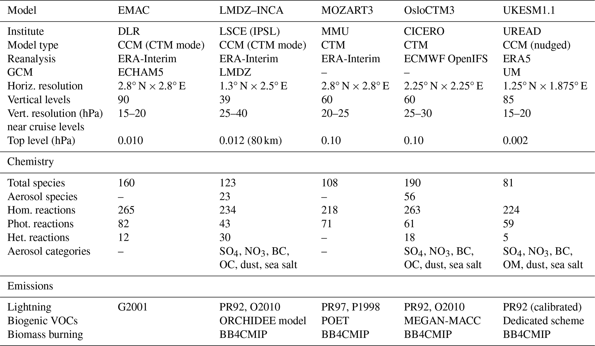
In this section, Table 1 summarizes the key model characteristics. In the next subsections (Sect. 2.2.1–2.2.5), further detail is given for each model, notably the tropospheric and stratospheric chemical schemes implemented in the models are described.
Table 1 Description of the participating models. In the first column, the abbreviations Horiz., Vert., Hom., Phot., and Het. denote horizontal, vertical, homogeneous, photolytic, and heterogeneous, respectively. Among the aerosol categories, SO4, NO3, BC, OC, and OM represent sulfate, nitrate, black carbon, organic carbon, and organic matter, respectively. With respect to the references, G2001 represents Grewe et al. (2001); PR92 and PR97 represent Price and Rind (1992) and Price et al. (1997), respectively; O2010 represents Ott et al. (2010); and P1998 represents Pickering et al. (1998).
2.2.1 EMAC
The ECHAM/MESSy Atmospheric Chemistry (EMAC) model is a numerical chemistry and climate simulation system that includes sub-models describing tropospheric and middle-atmosphere processes and their interaction with oceans, land, and human influences (Jöckel et al., 2010). It uses the second version of the Modular Earth Submodel System (MESSy2) to link multi-institutional computer codes. As described in Jöckel et al. (2016), MESSy is a software package providing a framework for a standardized, bottom-up implementation of Earth system models with flexible complexity (Modular Earth Submodel System). The core atmospheric model is the fifth-generation European Centre Hamburg general circulation model (ECHAM5; Roeckner et al., 2006). The physics subroutines of the original ECHAM code have been modularized and re-implemented as MESSy sub-models and have continuously been further developed. Only the spectral transform core, the flux-form semi-Lagrangian large-scale advection scheme, and the nudging routines for Newtonian relaxation remain from ECHAM. For the present study, we applied EMAC (MESSy version 2.55.2) at the T42L90MA resolution, i.e. with a spherical truncation of T42 (corresponding to a quadratic Gaussian grid of approximately 2.8° × 2.8° in latitude and longitude) with 90 vertical hybrid pressure levels up to 0.01 hPa. In ECHAM5, the nudging applies to vorticity, temperature, the logarithm of the surface pressure, and divergence, with the relaxation time being 6, 24, 24, and 48 h, respectively. The use of a so-called “quasi chemistry–transport mode” (QCTM; Deckert et al., 2011) enables binary identical simulations with respect to atmospheric dynamics and perturbations in chemistry to be detected with a high signal-to-noise ratio. The applied model set-up comprised the Module Efficiently Calculating the Chemistry of the Atmosphere (MECCA), which is used for tropospheric and stratospheric chemistry calculations with the possibility of extension to the mesosphere and oceanic chemistry (Sander et al., 2019). Reaction mechanisms include ozone, methane, HOx, NOx, non-methane hydrocarbons (NMHCs), halogens, and sulfur chemistry. Radiative transfer calculations are performed using the RAD sub-model (Dietmüller et al., 2016).
2.2.2 LMDZ–INCA
The LMDZ–INCA global chemistry–aerosol–climate model (hereafter referred to as INCA) is an online coupling of the LMDZ (Laboratoire de Météorologie Dynamique, version 6) general circulation model (Hourdin et al., 2006) and the INCA (INteraction with Chemistry and Aerosols, version 5) model (Hauglustaine et al., 2004). The interaction between the atmosphere and the land surface is ensured through the coupling of LMDZ with the ORCHIDEE (ORganizing Carbon and Hydrology In Dynamic Ecosystems, version 9) dynamical vegetation model (Krinner et al., 2005). In the present configuration, the model includes 39 hybrid vertical levels extending up to 70 km. The horizontal resolution is 1.25° × 2.5° (latitude × longitude). The primitive equations in the general circulation model (GCM) are solved with a 3 min time step, large-scale transport of tracers is carried out every 15 min, and physical and chemical processes are calculated at a 30 min time interval. For a more detailed description and an extended evaluation of the GCM, we refer to Hourdin et al. (2006).
INCA initially included a state-of-the-art CH4–NOx–CO–NMHC–O3 tropospheric photochemistry (Hauglustaine et al., 2004; Folberth et al., 2006). The tropospheric photochemistry and aerosol scheme used in this model version is described using a total of 123 tracers, including 22 tracers to represent aerosols. The model includes 234 homogeneous chemical reactions, 43 photolytic reactions, and 30 heterogeneous reactions. The gas-phase version of the model has been extensively compared to observations in the lower and upper troposphere. For aerosols, the INCA model simulates the distribution of aerosols with anthropogenic sources such as sulfates, nitrates, black carbon, and particulate organic matter, as well as natural aerosols such as sea salt and dust. Ammonia and nitrate aerosols are considered as described by Hauglustaine et al. (2014). The model has been extended to include an interactive chemistry in the stratosphere and mesosphere. Chemical species and reactions specific to the middle atmosphere were added to the model. A total of 31 species were added to the standard chemical scheme, mostly belonging to the chlorine and bromine chemistry, along with 66 gas-phase reactions and 26 photolytic reactions (Terrenoire et al., 2022; Pletzer et al., 2022).
In this study, meteorological data from the European Centre for Medium-Range Weather Forecasts (ECMWF) ERA-Interim reanalysis have been used to constrain the GCM meteorology and allow a comparison with measurements. The relaxation of the GCM winds toward ECMWF meteorology is performed by applying a correction term to the GCM zonal and meridional wind components at each time step, with a relaxation time of 3.6 h. The ECMWF fields are provided every 6 h and interpolated onto the LMDZ grid.
The ORCHIDEE vegetation model has been used for the offline calculation of the biogenic surface fluxes of isoprene, terpenes, acetone, and methanol as well as NO soil emissions, as described by Messina et al. (2016). The lightning NOx parameterization is described in Jourdain and Hauglustaine (2001). The lightning frequency follows the parameterization from Price and Rind (1992). In this simulation, a rescaling constrains the mean global flash rate at 46.3 flashes per year, consistent with the annual climatologies derived from both Lightning Imaging Sensor and Optical Transient Detector (LIS–OTD) satellite instruments in Cecil et al. (2014), from 1995 until 2010. This rescaling accounts for the different LIS- and OTD-sampled latitude bands and their different sampling periods. The lightning NOx (LNOx) emissions are then redistributed vertically, based on Ott et al. (2010).
2.2.3 MOZART3
Version 3 of the Model for OZone And Related chemical Tracers (MOZART3) is an offline global chemical transport model, extensively evaluated (Kinnison et al., 2007) and used for a range of various applications (Liu et al., 2009; Wuebbles et al., 2011), including studies dealing with the impact of aviation emissions on atmospheric composition (Søvde et al., 2014; Skowron et al., 2015). MOZART3 accounts for advection based on the flux-form semi-Lagrangian scheme (Lin and Rood, 1996), shallow and mid-level convection (Hack, 1994), the deep convective routine (Zhang and McFarlane, 1995), boundary layer exchanges (Holtslag and Boville, 1993), or wet and dry deposition (Brasseur et al., 1998; Müller, 1992).
The model reproduces detailed chemical and physical processes from the troposphere through the stratosphere. The chemical mechanism consists of 108 species, 218 gas-phase reactions, and 71 photolytic reactions (including the photochemical reactions associated with organic halogen compounds). The species included within this mechanism are members of the Ox, NOx, HOx, ClOx, and BrOx chemical families, along with CH4 and its degradation products. A NMHC oxidation scheme is also represented. The kinetic and photochemical data are based on the NASA/JPL Data Evaluation (Sander et al., 2006).
The horizontal resolution used in this study is T42 (2.8° × 2.8°), and the model domain spans 60 vertical layers between the surface and 0.1 hPa. The vertical resolution is 700–900 m at aircraft cruise altitudes (250–200 hPa). The transport of chemical compounds and the hydrological cycle are driven by the meteorological fields from the ERA-Interim 6 h reanalysis.
The surface and aviation emissions represent the years 2014–2018. The anthropogenic and biomass burning emissions are taken from CEDS version 2021 and GFEDv4, respectively, while the biogenic emissions are taken from POET (Granier et al., 2005). The parameterization of NOx emissions from lightning follows the assumption that the lightning frequency depends on the convective cloud-top height and the ratio of cloud-to-cloud versus cloud-to-ground lightning depends on the cold-cloud thickness (Price et al., 1997). The lightning NOx emissions are distributed vertically through the convective column according to observed profiles based on Pickering et al. (1998). The lightning source is scaled to provide a total of 4.7 Tg(N) yr−1, with daily and seasonal fluctuations based on the model meteorology. The patterns of the lighting NOx distribution in MOZART3 show a general agreement with LIS and OTD climatology datasets (Skowron et al., 2021). Simulations were preceded by a 1-year spin-up.
2.2.4 OsloCTM3
OsloCTM3 is an offline global chemical transport model driven by 3 h meteorological forecast data from the European Centre for Medium-Range Weather Forecasts (ECMWF) Integrated Forecast System (IFS) model (Søvde et al., 2012). The default horizontal resolution is 2.25°×2.25°, with an option to run at 1°×1°. In the vertical, the model has 60 levels, with the uppermost centred at 0.1 hPa. The model code is openly available from GitHub: https://github.com/NordicESMhub/OsloCTM3 (last access: 12 May 2022).
The chemistry of OsloCTM3 covers both tropospheric and stratospheric chemistry, treated by separate modules (Berntsen and Isaksen, 1997; Stordal et al., 1985). The tropospheric code is stand-alone, but the stratospheric code needs the tropospheric chemistry module to work. The kinetics are based on JPL 2006 (Sander et al., 2006), while the photodissociation coefficients are calculated online using the Fast-JX scheme (Prather, 2009). The numerical integration of chemical kinetics is done by applying the quasi-steady-state approximation (QSSA; Hesstvedt et al., 1978), using three different integration methods depending on the chemical lifetime of the species. The model also treats the main anthropogenic and natural aerosol species (sulfate, nitrate/ammonium, black carbon, primary and secondary organic aerosol, dust, and sea salt). The aerosol schemes are described in more detail in Lund et al. (2018).
The model transport covers large-scale advection treated by the second-order moment (SOM) scheme (Prather, 1986), convective transport based on Tiedtke (1989), and boundary layer mixing based on Holtslag et al. (1990). Scavenging covers dry deposition, i.e. uptake by soil or vegetation at the surface, and washout by convective and large-scale rain (Søvde et al., 2012).
For ACACIA, the output is made of a succession of 1-year simulations, each one with a 6-month spin-up. Anthropogenic emissions are from CEDS (version 2021) with GFEDv4 biomass burning and MEGAN-MACC year 2010 biogenic emissions. Lightning NOx emissions are calculated online (Søvde et al., 2012), as are dust and sea salt fluxes (Lund et al., 2018, and references therein).
Lightning NOx emissions are calculated from the convective fluxes provided by the meteorological input data using the algorithm based on cloud-top height from Price and Rind (1992), with a scaling that matches lightning flash rates observed by OTD and LIS. The in-cloud flash rate depends on whether the surface is land or ocean. The model distributes LNOx emissions vertically through the convective column according to observed profiles (Ott et al., 2010) for four world regions. These profiles are scaled vertically to match the height of each convective plume in the CTM and already account for the vertical mixing of lightning NOx within the cloud. Geographic region definitions are from Allen et al. (2010) and Murray et al. (2012).
2.2.5 UKESM1.1
The UK Earth System Model version 1 (UKESM1; Sellar et al., 2019) is a global climate model made by coupling atmosphere, ocean, sea ice, and land surface models. In this study, UKESM1 is used in its atmosphere-only configuration, where ocean sea surface temperature and sea ice distributions are prescribed from previous simulations with the fully coupled model. The atmosphere model is built on the Met Office Unified Model (Walters et al., 2019), decomposing the atmosphere in 85 terrain-following hybrid vertical levels up to an altitude of 85 km. The horizontal resolution is 1.25°×1.875°.
Atmospheric chemistry is simulated by the stratosphere–troposphere StratTrop chemistry scheme (Archibald et al., 2020) of the UK Chemistry and Aerosols (UKCA) sub-model. StratTrop unifies two originally separate tropospheric and stratospheric chemistry modules, described by O'Connor et al. (2014) and Morgenstern et al. (2009), respectively. StratTrop simulates Ox, HOx, and NOx chemistry based on 15 emitted species (including NO, CO, and aerosol precursor gases) and 7 long-lived species (including CH4), which are constrained by surface concentrations. Tracer advection, convective transport, and boundary layer mixing are simulated by the Unified Model (Walters et al., 2019). Wet deposition follows Giannakopoulos et al. (1999), while dry deposition depends on the surface types simulated by the land surface model, as described in Archibald et al. (2020). Photolysis rates are computed interactively by the Fast-JX scheme (Neu et al., 2007) depending on three-dimensional radiation. In terms of aerosols, UKCA simulates the mass and number of sulfate, nitrate, black carbon, primary and secondary organic, mineral dust, and sea salt aerosols (Mulcahy et al., 2018). Horizontal winds are nudged with a relaxation time of 6 h.
Lightning NOx emissions are described in Sect. 2.6.3 of Archibald et al. (2020). They are calculated following Price and Rind (1992), where lightning flash density depends on cloud-top height and surface type (land or ocean). The scheme distinguishes the energy discharged by cloud-to-cloud and cloud-to-ground flashes and uses a spatial calibration factor to make the scheme independent of model resolution. The scheme is only applied when the cloud depth reaches at least 5 km according to the convection scheme. NOx emissions are distributed linearly with the logarithm of pressure. They have been calibrated to reach an average global annual emission rate of 5.98 TgN yr−1 over the period from 2005 to 2014.
In this study, UKESM1 simulated the period from 1990 to 2018, using CMIP6 historical and, from 2015 onward, SSP3-7.0 emissions as monthly distributions. The CMIP6 aircraft emission inventories were corrected for the mistake identified by Thor et al. (2023). Emissions of sea salt and mineral dust aerosols and biogenic VOCs are interactive. The model was nudged to 6 h horizontal wind speed distributions from ERA5.
2.3 The IAGOS data
The IAGOS research infrastructure (http://www.iagos.org, last access: 1 November 2022) provides long-term routine in situ observations of chemical species aboard a fleet of several passenger aircraft. Its predecessors – MOZAIC (Measurements of water vapor and OZone by Airbus In-service airCraft; Marenco et al., 1998) and CARIBIC (Civil Aircraft for the Regular Investigation Based on an Instrument Container; Brenninkmeijer et al., 1999, 2007; Stratmann et al., 2016) – relied on the same principle. The MOZAIC measurements began aboard five equipped aircraft measuring ozone and water vapour in August 1994. CO observations began in December 2001, and NOy measurements were operational on one aircraft between April 2001 and May 2005. CARIBIC has sampled a wide variety of atmospheric species since 1997 from one single aircraft, including those measured by MOZAIC. Since the mergence of the two programmes in 2008, their respective databases are referred to as IAGOS-CORE and IAGOS-CARIBIC. In the present study, we consider them as a single database called IAGOS hereafter, an approach validated by Blot et al. (2021) for ozone and CO. The period that we are analysing spreads from August 1994 until December 2017, hence the 1994–2017 (or 2001–2017) period covered by the models' run. The most sampled altitudes are between 180 and 310 hPa, and the vertical distribution of sampling varies geographically. The methodology used for the models' assessment using the IAGOS data is described in Sect. 2.4.
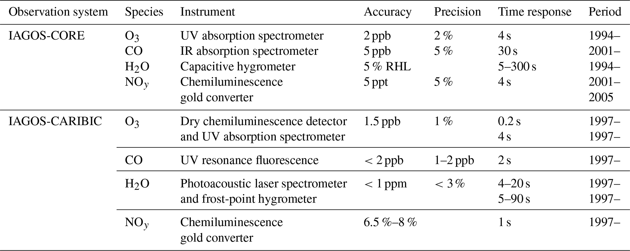
The main characteristics of the IAGOS instruments relevant to this study are indicated in Table 2. Concerning the IAGOS-CORE instruments, further information is available in Thouret et al. (1998) for ozone; in Nédélec et al. (2003) and Nédélec et al. (2015) for CO; in Helten et al. (1998), Neis et al. (2015a), Neis et al. (2015b), and Rolf et al. (2023) for water vapour; and in Volz-Thomas et al. (2005) and Pätz et al. (2006) for NOy. Note that the IAGOS-CORE water vapour measurements have an accuracy of 6 % RHL (relative humidity with respect to liquid water) in the vicinity of the midlatitude thermal tropopause (Smit et al., 2014; Petzold et al., 2020). Due to a moist bias in the IAGOS-CORE H2O observations for the driest air masses (RHL <5 %) which are encountered in the lower stratosphere, this study does not quantify the model H2O biases in regions other than the upper troposphere. Concerning the IAGOS-CARIBIC instruments, further information is available in Zahn et al. (2012) for ozone, in Scharffe et al. (2012) for CO, in Zahn et al. (2014) and Dyroff et al. (2015) for water vapour, and in Ziereis et al. (2000) and Stratmann et al. (2016) for NOy. More precisely, the latter has a total measurement uncertainty of 6.5 % (8 %) for a measured mixing ratio of 1 ppb (0.5 ppb). For both programmes, the time response of the water vapour sensors decreases with the measured water content.
Table 2 Characteristics of the IAGOS instruments measuring ozone, CO, water vapour, and NOy. The last column shows the time period covered by the measurements. The periods ending with an en dash (–) mean that the measurements are still ongoing.
2.4 Methodology for assessing modelled mixing ratios of chemical species in the UTLS
The Interpol-IAGOS software (Cohen et al., 2021) aims to facilitate the assessment of the model output with the IAGOS data by deriving two respective products that are directly comparable. It consists of a projection of the scattered IAGOS data onto the regular model grid, day by day, followed by a monthly average. For a given model, the subsequent gridded IAGOS product is then denoted as the “IAGOS–DM–model”, with the “–DM” suffix referring to the distribution onto the model grid. For further simplicity in this study, we refer to it as “IAGOS–model”, and the IAGOS–DM–model products in their ensemble are called “IAGOS–DM products”. Concerning the model output, a daily mask is applied with respect to the IAGOS sampling (Cohen et al., 2023), excluding the non-sampled daily grid points. This way, the subsequent monthly products are representative of the same grid points and the same days. As in Cohen et al. (2023), their whole name is “model–M” (with the “–M” suffix referring to the IAGOS mask); except in this section where there can be confusion, we refer to them simply using the model name. The monthly average is calculated for each layer separately. This implies that a monthly average is calculated for both layers for each grid cell included in both the UT and LS during a month. Finally, the seasonal and annual climatologies are then derived from the monthly means with the same method and filtering as in Cohen et al. (2023). For each model, the IAGOS–DM–model and model–M product pairs are, thus, representative of the same time period as well.
For each model, the tropopause is defined dynamically as the isosurface of 2 PVU (potential vorticity units) derived from the model output. The UT spreads from 400 hPa up to the tropopause level but excludes the top grid cell in order to avoid the strongest mixing zone, directly impacted by both layers (e.g. Thouret et al., 2006; Cohen et al., 2018). The LS corresponds to all of the sampled grid cells above the 3 PVU isosurface. In order to limit the impact of errors in the modelled PV on the evaluation, we exclude cases in which the modelled PV value and the daily average of the observed ozone mixing ratios are very likely to represent different layers. As in previous studies (Cohen et al., 2021, 2023), a daily grid cell in the UT (LS) is filtered out when the average ozone from IAGOS is more than 140 ppb (less than 60 ppb). Finally, the non-separated UTLS represents all of the measurement points above 400 hPa, and it has been added to this paper in order to include the output from the MOZART3 model without a PV field. In the tropics, the tropopause altitude does not allow the aircraft to sample stratospheric air masses. Consequently, only the UT is represented between 25° S and 25° N, and it includes all of the measurements above 300 hPa, although the uppermost part of the tropical troposphere remains higher than cruise altitudes. In the framework of the CCMI modelling experiment, Orbe et al. (2020) reports that the nudging process tends to enhance the transport variability between the CCMs and can generate artificial transport in regions of strong gradients. This issue might be partly addressed by our methodology, notably the definition of the layers, which enhances the isolation between them, and the exclusion of the grid cells with an inconsistent PV value with respect to the ozone observations. The mean pressure differences between observations and the model 2 PVU tropopause shown in Supplement (Figs. S1–S5) do not exhibit noticeable variations between the models: mostly, they are less than 5 hPa (except in winter and spring for ozone and NOy), and they are always less than 10 hPa. It might still be problematic for water vapour in the LMS, as the vertical gradient from the tropopause is particularly high, including 2 orders of magnitude (Zahn et al., 2014), but, as described above, the model skills do not cover water vapour in the LMS. For each species and layer, the distance between the sampled grid cells and the tropopause does not vary enough across the models to play a significant role in the inter-model discrepancies, as there is no visible correlation with the chemical tracers.
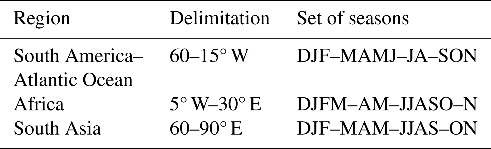
As in Cohen et al. (2023), the chosen metrics are the modified normalized mean bias (MNMB), the fractional gross error (FGE), and Pearson's correlation coefficient, all defined in Supplement (Eqs. S1–S4). As the models have different PV fields and some of them have a different time period, each model is compared to its own IAGOS–model reference product. This study is divided into comparisons in the extra-tropics and in the tropics. The results in the extra-tropics are generally represented with several sets of metrics (quantiles, biases, and linear regression metrics). On the contrary, as the sampling in the tropics is more heterogeneous, three regions have been chosen, as in Cohen et al. (2023), and are represented by the mean zonal cross sections: western Atlantic–South America (called South America hereafter), Africa, and South Asia. As a compromise between an efficient sampling and spatial uniformity for the observed species, their respective zonal cross sections are averaged through the following longitude bands: 60–15° W, 5° W–30° E, and 60–90° E. For each of these regions, the year is divided into seasons that depend on the mean position of the Intertropical Convergence Zone (ITCZ). As in Cohen et al. (2023), the tropical season definitions were based on the months with the northernmost and southernmost position of the ITCZ (located with the observed horizontal winds and water vapour), as an extension of Lannuque et al. (2021), who focused on Africa. They are summarized in Table 3, taken from Cohen et al. (2023).
This section is divided into two approaches. We first present introductory results showing global annual maps of model mean biases. We then more precisely treat the northern extra-tropics in the UT and the LS separately and, to a lesser extent, in the non-separated UTLS. Finally, we move into the (sub-)tropical UT characterization. It is worth again noting that the principal criterion for the UT and LS definition beyond ±25° N is the 2 PVU isosurface from the nudged CCMs/forced CTM and that the tropical UT comprises every sampled grid cell above 300 hPa (as our sampling does not reach the tropical tropopause layer).
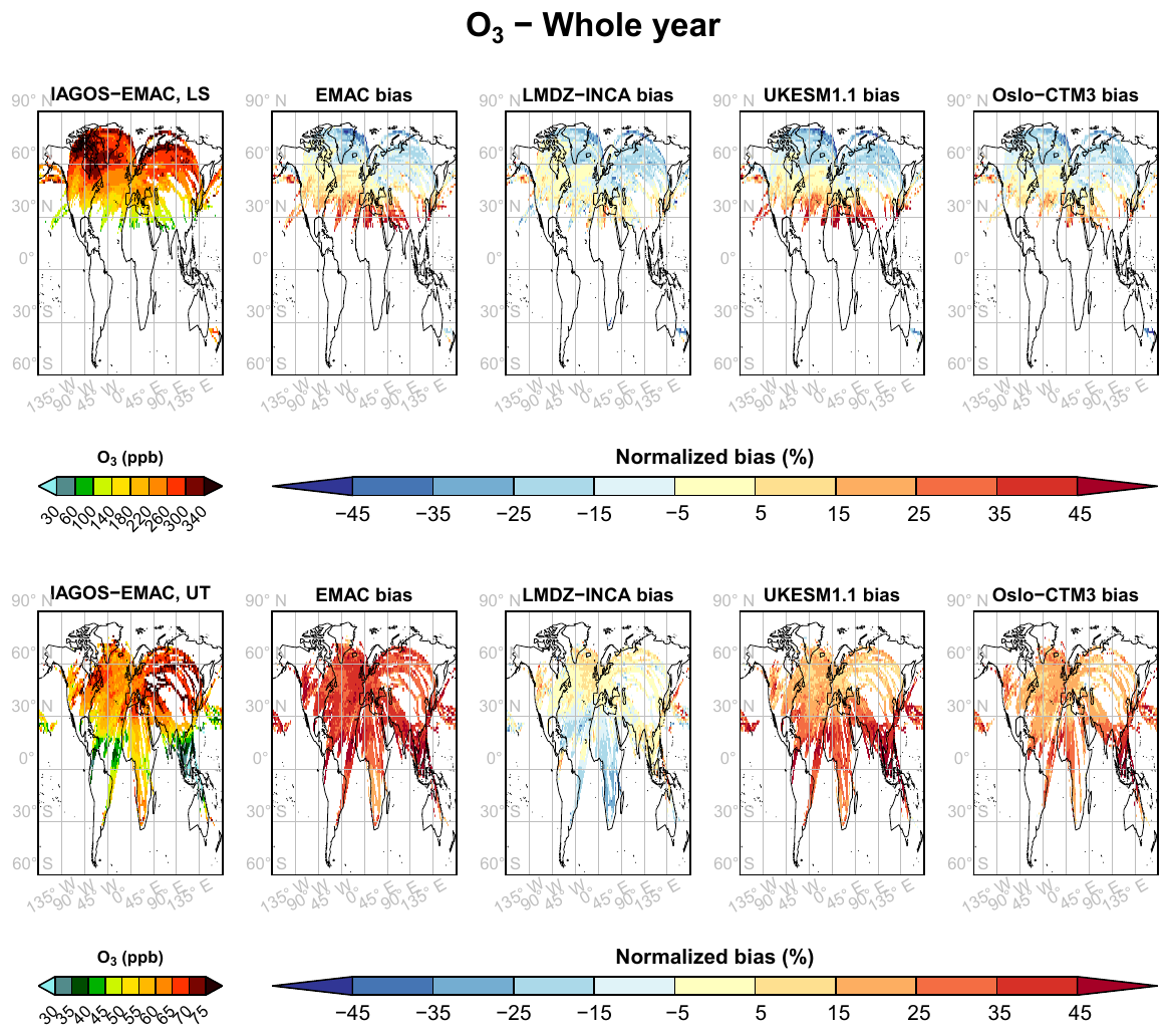
Figure 1The panels in the first column show the ozone mean horizontal distributions of annual averages from December 1994 until November 2017 for the IAGOS–EMAC product, whereas the other panels (the second to fifth columns) present the respective biases for the masked output from EMAC, LMDZ–INCA, UKESM1.1, and OsloCTM3 normalized with respect to the mean values between each model output and their corresponding IAGOS–DM product. The bottom row shows the UT, whereas the top row presents the LS.
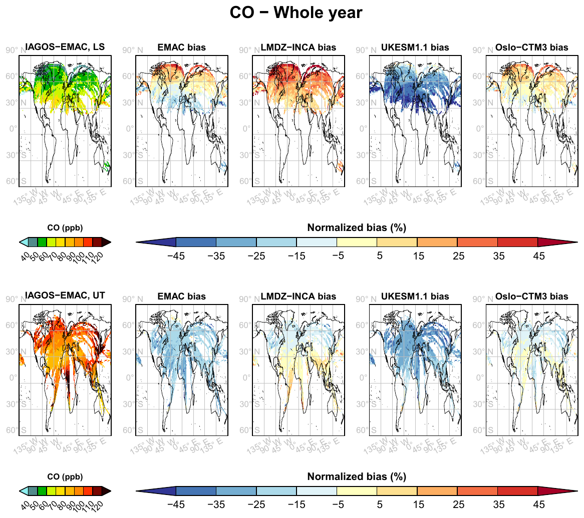
Figure 2Same as Fig. 1 but for carbon monoxide from 2002 to 2017.
3.1 Horizontal distributions
The annual climatologies of the model biases in the UT and the LS are shown in Figs. 1–4 for the four models with an available PV field. A climatology is also shown for one of the gridded IAGOS products (hereafter referred to as “IAGOS–DM products”; see Sect. 2.4) in order to provide a view of the expected features, but each bias remains relative to a different IAGOS–DM product, notably due to the different time periods. As the IAGOS–DM climatologies are relatively similar through the simulations with the same duration (not shown), we chose only one of the IAGOS–DM climatologies with the longest time period (by default IAGOS–EMAC, i.e. the gridded IAGOS product on the EMAC model's grid, as explained in Sect. 2.4). We note the sampling differences between the climatologies from OsloCTM3 (2001–2017) and the other three assessed models (1994–2017). Interannual variability is, therefore, likely to cause moderate differences in the observed climatologies for ozone and water vapour in OsloCTM3, the time period of which is 25 % shorter than for the other models. This does not apply to CO and NOy, as their IAGOS-CORE observations started in 2001.
On a yearly average, we first notice common features between the models. The four models exhibit a geographical anticorrelation between ozone and CO biases in the LS (Figs. 1 and 2). The ratio shown in Fig. A1 summarizes this pattern well, with the MNMB decreasing with latitude. On the other hand, upper-tropospheric ozone is overestimated in the midlatitudes, whereas CO tends to be underestimated. These combined features suggest that the four models tend to overestimate the overall impact of stratosphere–troposphere exchanges across the extratropical tropopause. Most of the models also overestimate ozone in the tropics, which is analysed in detail in Sect. 3.3. We can notice that the models showing a more positive (negative) bias in ozone (CO) in the low-latitude LS have the same tendency in the tropical UT, possibly as an impact of isentropic cross-tropopause exchanges that can extend biases to the adjacent layer. Figure 3 shows that, contrary to the other species, each model NOy climatology is simultaneously characterized by both low and high biases as well as a few grid cells with a weak bias. The map derived from the observations is heterogeneous too, with upper-tropospheric minima over Northwest America, the North Atlantic corridor, and near the Azores anticyclone (less than 400 ppt). A regional-scale maximum is visible over Northeast America (800–1400 ppt) and tropical Africa. The four models generally underestimate the magnitude of these geographical extrema, showing overly small variability. Finally, in Fig. 4, upper-tropospheric water vapour tends to be underestimated in the northern extra-tropics and, at least, in the northern tropics.
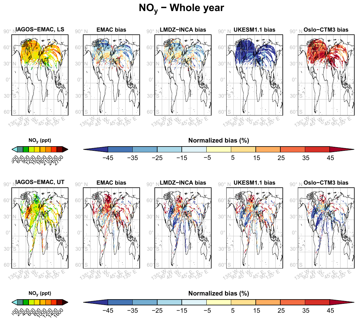
Figure 3Same as Fig. 1 but for nitrogen reactive species over the period from 1997 to 2017, although with more frequent sampling over the period from 2001 to 2005.
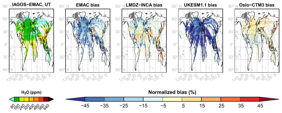
Figure 4Same as Fig. 1 but for water vapour in the upper troposphere.
3.2 Northern extra-tropics
In this subsection, we compare and characterize the observed and modelled seasonal cycles together. We then show synthesizing metrics to assess the model geographical distributions in the extra-tropics. Figures 5–8 provide an overview of the seasonal climatologies in the UT and the LS, and Fig. 9 presents the same information for the non-separated UTLS. Please note that observed lower-stratospheric water vapour in Fig. 5 is displayed as an indication of the seasonality; however, for the reasons explained in Sect. 2.3, some of its values are probably overestimated, and it cannot be used for a bias quantification. The height of the box plots illustrates the geographical variability. Water vapour seasonality in the UT (shown in Fig. 5) is well approximated in the simulations, with a wintertime minimum and a summertime maximum directly linked with convection and temperature, the latter of which governs saturation vapour pressure. The LS shows a similar pattern, although the contrast between the summertime water vapour maximum and the rest of the year is more pronounced than in the UT. This feature is consistent with the increased impact from the troposphere during this season and the extremely steep vertical gradient in water vapour. Based on CARIBIC measurements between 2005 and 2013, Zahn et al. (2014) found that the summertime maximum was primarily due to shallow cross-tropopause mixing in the extra-tropics. This takes place during the whole year; thus, the summertime H2O maximum in the UT increases the upward moisture flux. The other two pathways for moisture transport into the LS, i.e. localized deep convection events and, higher in the LS, quasi-isentropic mixing with the tropical transition layer (TTL), mostly take place during summer (and early autumn for the latter), but they were found to have a lesser contribution to the summertime moisture maximum.
The models have more difficulties in reproducing CO seasonality, according to Fig. 6. The observed springtime peak has been explained by an accumulation of CO in the lower troposphere during winter followed by an increase in the convective transport during spring (Cohen et al., 2018), allowing the lower-tropospheric CO reservoir to impact the UT. This springtime maximum is not visible in the simulations; its magnitude is underestimated as well, and contrary to the observations, the springtime distribution is similar to winter, a feature that extends up to the LS. The comparison with the realistic water vapour cycles in the UT tends to exclude convective transport from the causes of this discrepancy, except pyroconvection. It is possible that CO lifetime or CO emissions are underestimated, which reduces the wintertime accumulation in the lower troposphere and then the upward CO flux during spring. The lower values in the two tropospheric tracers (H2O and CO) in both the UT and LS with UKESM1.1 suggest an underestimation in the upward fluxes from the surface up to the UT, which favours an underestimation in the LS too.
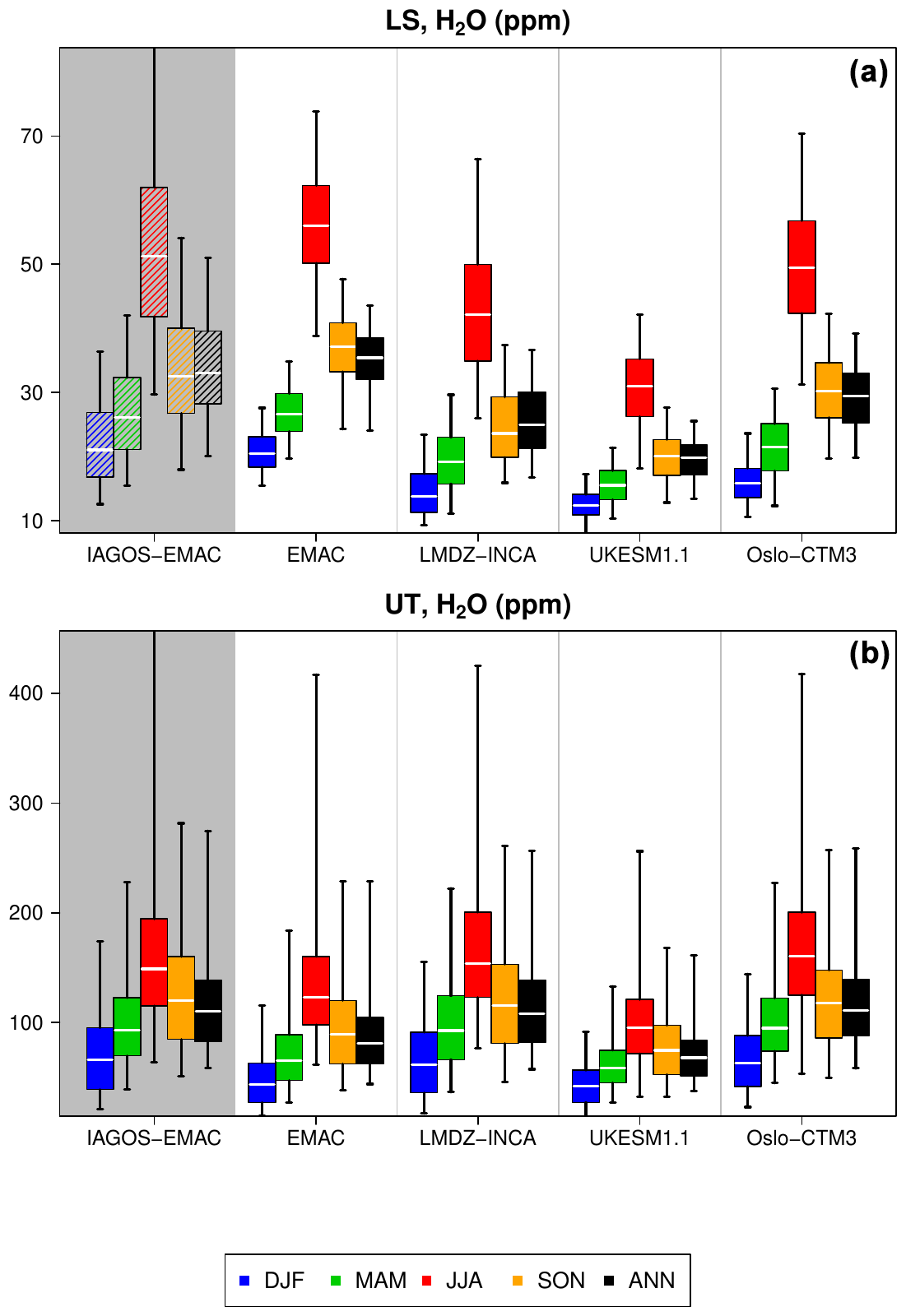
Figure 5Box plots synthesizing the mean geographical distribution of extratropical water vapour in the LS (a) and the UT (b) for the IAGOS–EMAC product and for the model products (from left to right). Each colour corresponds to a season, and the black boxes represent the annual means. For a given box plot, the white line represents the median, the box corresponds to the interquartile interval, and the whiskers represent the values between the 5th and 95th percentiles. Please note that, due to its uncertainty, the observed H2O in the LS shown here cannot be used for accurate quantification; therefore, it is shown using hatched box plots.
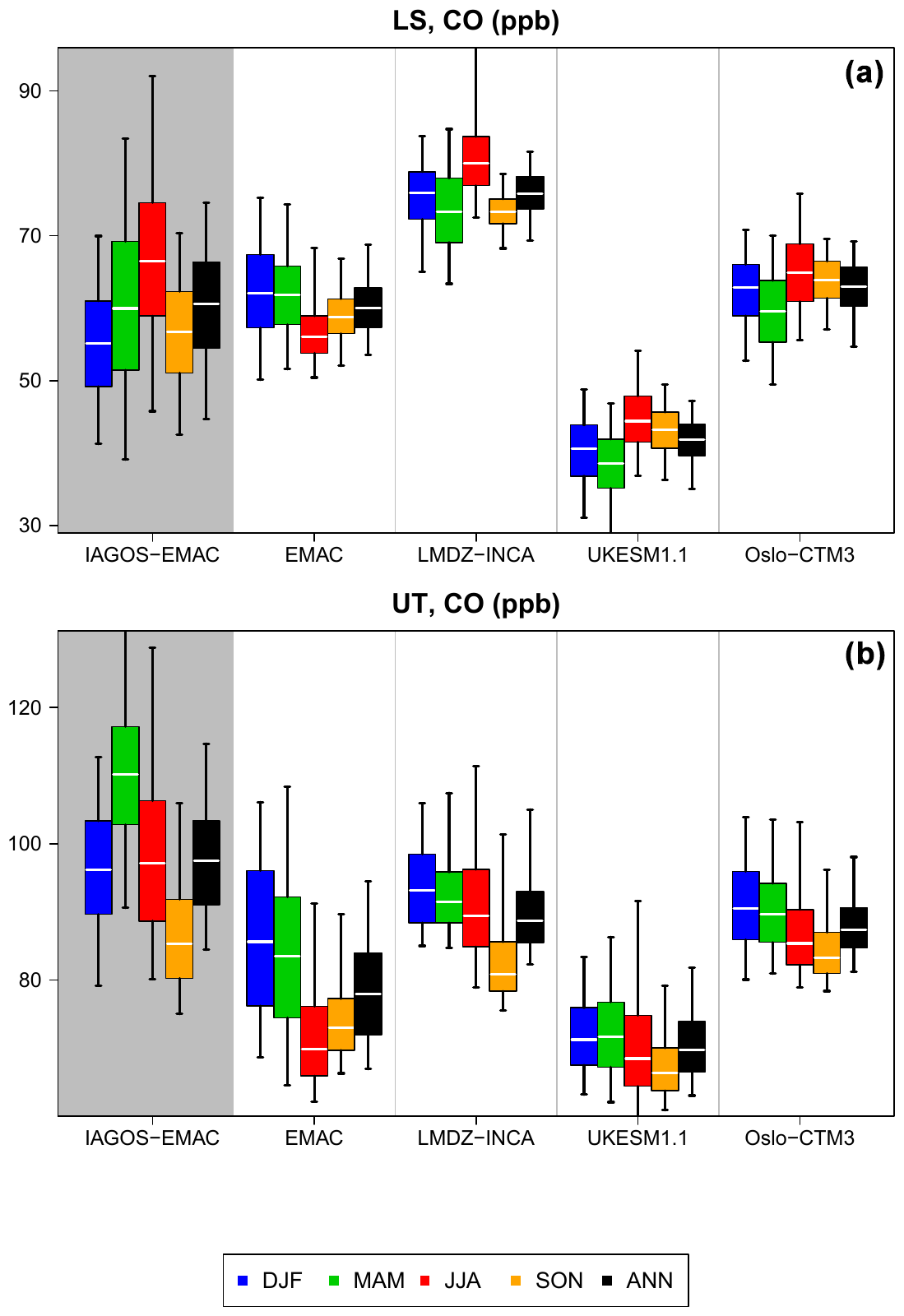
Figure 7 shows that the ozone maximum in the upper troposphere takes place in summer, with a peak in photochemical activity, whereas the minimum occurs during winter. In the lowermost stratosphere, the ozone maximum takes place during spring due to the effects of the descending branch of the Brewer–Dobson circulation, which transports ozone-rich air masses down from the deeper extratropical stratosphere, whereas the minimum takes place during autumn. The models reproduce well these features and the dichotomy in the UT between high-ozone seasons (spring and summer) and low-ozone seasons (winter and autumn). Although most models are positively biased, the magnitude of the seasonal cycle is similar to the observations. In the LS, the ozone distribution is harder to reproduce during summer and autumn, with a geographical variability only spreading over the lower half of the observed distribution. It is characterized by a tendency to overestimate the low-latitude ozone minima and underestimate the high-latitude ozone maxima (e.g. Fig. 1). Similarly to ozone, both observed and modelled NOy mixing ratios show a springtime maximum in the LS and a summertime maximum in the UT. In the UT, the summertime maximum is linked to photochemical activity, enhanced lightning frequency, more intense boreal forest fires, and enhanced convection that uplifts diverse ozone precursors from the lower troposphere. This is consistent with the detailed individual NOy species in Figs. B1–B3, where each of the models generally shows a summertime maximum in NOx, PAN, and (especially) HNO3. The latter is notably affected by the conversion from NOx via photochemical activity (Stratmann et al., 2016). In the LS, the impact of the Brewer–Dobson circulation coupled with HNO3 production from nitrous oxide decomposition in the stratosphere is reproduced, as shown in Fig. B3. The only exception is the UKESM1.1 model, which instead shows an upper-tropospheric seasonality in the LS, although the influence of the Brewer–Dobson circulation remains visible through more elevated springtime mixing ratios compared to the UT seasonal cycle. On the contrary, the OsloCTM3 model shows higher NOy values in the LS. As ozone amounts are within the same range as the other models, it excludes stratospheric circulation from the possible causes of NOy discrepancies. Thus, for UKESM1.1 (OsloCTM3), the lower (higher) HNO3 values in the LS (Fig. B3) might be due to an underestimation (overestimation) of N2O flux into the stratosphere, an overestimated (underestimated) N2O lifetime in the stratosphere, or an underestimated (overestimated) HNO3 lifetime against stratospheric aerosol uptake. The latter is a possible contributor for OsloCTM3, as its mass density of particular sulfate and nitrate is 10 % lower than in the LMDZ–INCA simulation. Lower NOy and HNO3 mixing ratios in UKESM1.1 are unlikely due to the different representation of the Brewer–Dobson circulation in the reanalyses, as the mean age of air in the northern LS is longer in ERA5 than in ERA-Interim (Ploeger et al., 2021; Li et al., 2022), which would tend to convert more N2O into HNO3 in UKESM1.1. In the end, considering both ozone and NOy in the LS, the similarities between observations and models, notably during spring, are encouraging with respect to the stratospheric chemistry and diabatic transport for all of the models.
As shown in Figs. B1–B2 and B4, NOy partitioning changes substantially between the models. In the UT, a higher proportion of NOy is represented by HNO3 with OsloCTM3. As it is affected by wet scavenging, it can explain the lower NOy mixing ratios with this model, combined with very low PAN quantities. On the contrary, the higher levels of NOy in the UT with the EMAC model can be linked to the high proportion of PAN which is not soluble and has a chemical lifetime of several months (e.g. Fadnavis et al., 2015). The higher amount of PAN might inherently be linked to the colder EMAC temperatures ( K), as it increases its lifetime against thermolysis. In the UT, the higher (lower) NOx mixing ratios from the EMAC (LMDZ–INCA) model can also explain the higher (lower) ozone mixing ratios. The inter-model variability with respect to PAN in the UT might also have consequences for the air quality evaluation in the subsidence regions, as the PAN lifetime against thermolysis decreases drastically during descending motion, from months down to minutes when the temperature reaches 20 °C. Regarding this variability, surface ozone production due to PAN subsidence is, thus, likely to vary substantially across the models (at least in remote areas with a NOx-limited regime), with a maximum for EMAC and a minimum for OsloCTM3. In the LS, PAN inter-model variability is the most noticeable of all NOy species, with a factor reaching 12 between the median mixing ratio from EMAC and OsloCTM3 and an important difference in every couple of models. The low (high) amounts of PAN simulated with OsloCTM3 (EMAC) are, at least partially, related to the low (high) amounts in the UT as well.
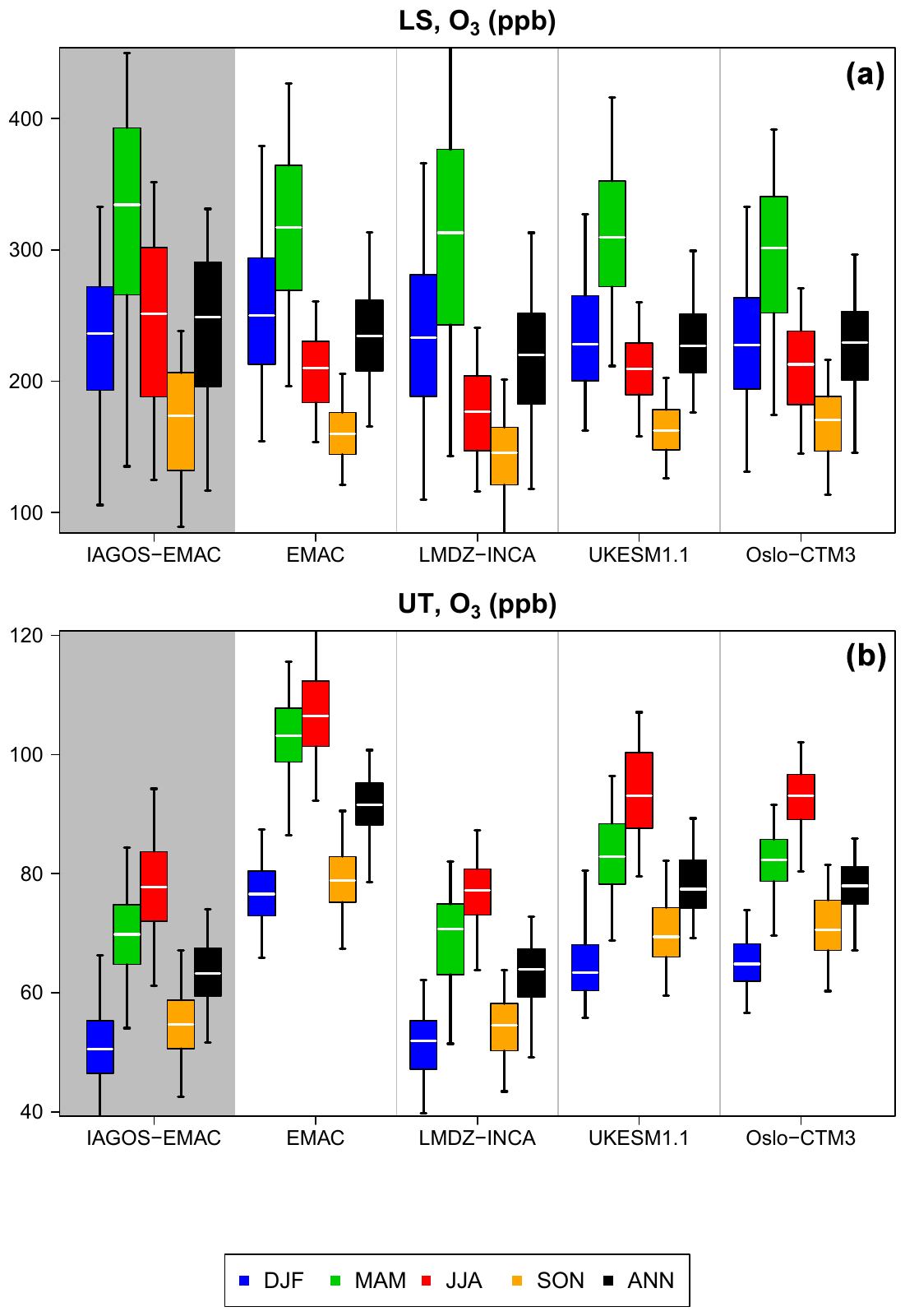
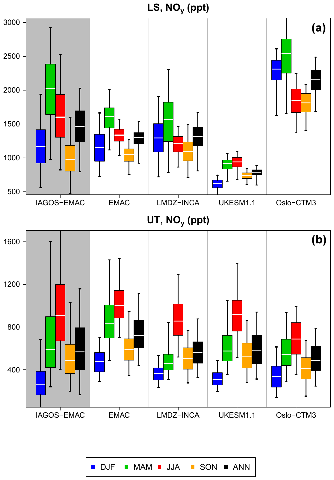
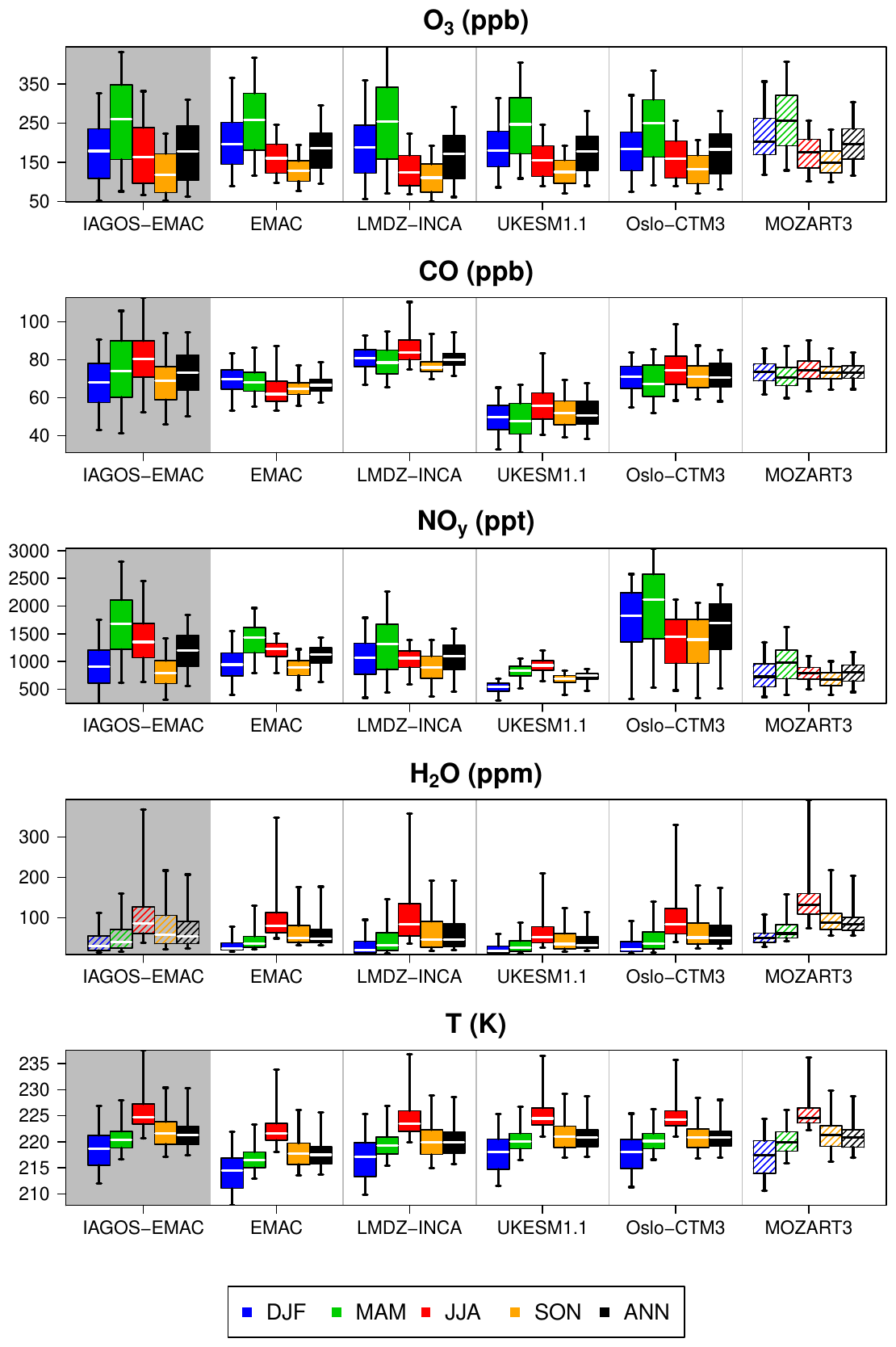
Figure 9Box plots synthesizing the mean geographical distribution of extratropical variables (from top to bottom, ozone, CO, NOy, water vapour, and temperature) in the non-separated UTLS for the IAGOS–EMAC product and for the five model products (from left to right). Due to its uncertainty, observed H2O in the LS shown here cannot be used for accurate quantification, hence the hatched IAGOS–EMAC box plots. Box plots are also hatched for MOZART3 to remind the reader that the corresponding climatologies cannot be compared directly to the IAGOS–EMAC product, as it is based on a different meteorology.
The lower-stratospheric features described above are generally visible in the UTLS as well, as illustrated in Fig. 9, for the species with a strong positive vertical gradient. Notably, the springtime maximum is well represented by every model for ozone and almost all of the models for NOy, including MOZART3, which confirms that all of the models catch the seasonality of the Brewer–Dobson circulation. The water vapour and temperature maxima in summer are also visible in the simulations. For the five models, the NOy seasonal cycle is characterized by a springtime maximum in HNO3, due to the Brewer–Dobson circulation, and by a summertime maximum in both NOx and PAN, due to convection, photochemistry, and lightning emissions.
In Figs. 7–9, we note that, when they are noticeably biased, the sign of the annual mean bias is generally representative of all of the seasons, although its magnitude is not. With this perspective, the annual means shown below still provide relevant information. Figure 10 synthesizes some model skills in terms of annual averages in the extra-tropics, and the inter-model ranges are indicated more precisely in Table 4. The ozone mixing ratio is generally more difficult to model in the UT than in the LS, in terms of the geographical distribution (rUT(O3) =0.45–0.74, compared to rLS(O3) =0.75–90) as well as in terms of the mean biases, with the latter being essentially positive for most models in the UT (MNMB =0.005–0.36 and FGE ∼ MNMB for three models) and weak in the LS (MNMB –0.006, with a maximum FGE at 0.16, which is particularly low). On the contrary, the CO correlation coefficient is higher in the UT (rUT(CO) =0.63–0.78) than in the LS (rLS(CO) =0.11–0.70), probably reflecting the difficulty in mapping the effects of cross-tropopause exchange. In the UT, ozone and CO biases tend to be positive and negative, respectively. This difference can be linked to overestimated cross-tropopause exchange and/or overestimated photochemical activity, thus more ozone production and more CO destruction. In the UT, both surface tracers (CO and H2O) also show good correlations (rUT(H2O) ∼0.95 and, for most models, rUT(CO) ∼0.8). The skill difference between the two species can be explained by either uncertainties in CO emissions in each region or an underestimation of the detrainment altitude from pyroconvection, consistent with the negative biases in CO in the UT. Interestingly, the bias magnitudes for both species are higher for EMAC and UKESM1.1. Concerning EMAC, the systematically negative temperature biases (−3.7 K on average) could be another factor controlling lower water vapour amounts in the UT via saturation, but this would not be consistent with the combination of lower temperatures (−4.0 K on average) with more water vapour in the LS, compared to the other models. A comparable cold bias with EMAC has been diagnosed in Righi et al. (2015) with a similar simulation set-up; this prior study also identified a wet bias compared to the observations from the Halogen Occultation Experiment (HALOE; Grooß and Russell III, 2005) at 200 hPa in the extra-tropics. They concluded that an overestimation of lower-stratospheric water vapour would cause excessive radiative cooling and, thus, a cold bias – a relation that had already been shown in previous studies. This moisture overestimation in the LS is confirmed in Fig. 5, showing higher H2O amounts in EMAC compared to the observations, given that the latter are probably overestimated. Concerning UKESM1.1, it is worth reiterating that the low mixing ratios in H2O and CO in both layers (see Figs. 5 and 6) suggest an underestimation in the upward fluxes from the surface up to the UT. Finally, NOy shows the largest variability in the MNMB in the UT and the lowest correlation coefficient among the four chemical species. This could be due to the important inter-model variability in the spatial distribution of lightning emissions (e.g. Hakim et al., 2019) or to the washout of HNO3, the latter of which depends on the cloudiness representation and NOy partitioning.
Table 4Annual metrics synthesizing the assessment of O3, CO, the O3 CO ratio, NOy, H2O, and temperature climatologies from the model simulations against their respective IAGOS–DM product in the UT and the LS, as shown in Fig. 10 and the Appendix (Figs. A2–A5). From left to right, the Pearson correlation coefficient (r), the modified normalized mean bias (MNMB), the fractional gross error (FGE), and the sample size (Ncells) are shown. For temperature, the absolute bias and its associated error are equivalent to the MNMB and the FGE without the normalizing factors. Each metric is represented with an inter-model range.
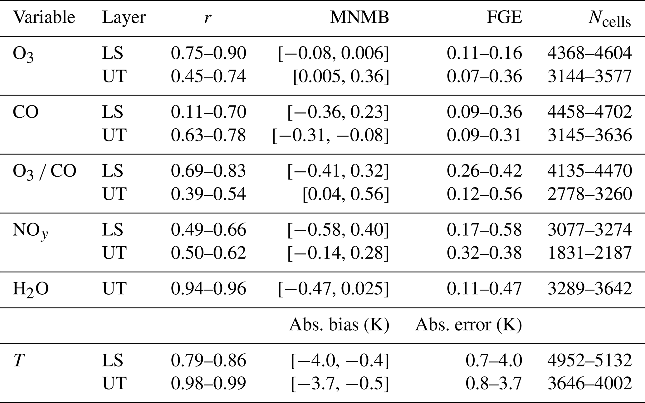
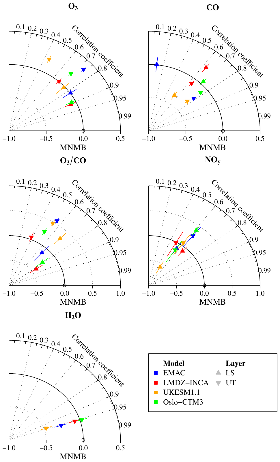
Figure 10Modified Taylor diagrams synthesizing the assessment of the yearly climatologies beyond 25° N derived from the five models' output against their respective IAGOS–DM product for O3, CO, the O3 CO ratio, NOy, and upper-tropospheric H2O. Each model is represented by a colour and each layer by a point shape. The radial axis corresponds to the modified normalized mean bias (MNMB) for the chemical compounds, whereas the orthoradial axis refers to the r correlation coefficient. The error bars are quartiles 1 and 3 of the normalized biases shown in Figs. 1–4.
Figures A2–A5 provide further information on the annual geographical distribution mentioned above for each species, layer, and model in the northern extra-tropics. The particularly high correlation for water vapour (r=0.95) shown in Fig. A2 is characterized by a well-reproduced meridional structure, notably with strong variability in the lowest latitudes (orange and red dots) due to dry subsiding and moist convective regions. This is notably characterized by a linear regression slope close to 1 for EMAC, LMDZ–INCA, and OsloCTM3. All of these features are representative of all of the seasons, with the highest correlation and linear regression slope during summer, when the tropospheric humidity reaches its maximum. These features are encouraging with respect to the modelled impact of meteorological systems on the extratropical UT in terms of geographical variability, despite the negative mean biases present in most models.
In the lowermost stratosphere, Fig. A3 shows that ozone geographical variability is relatively well reproduced by the models with a distinct northward gradient. This gradient tends to be underestimated because of a positive bias in the lowest values (in the subtropics) for most models and a negative bias in the highest values in the subpolar regions. The northward gradient is also visible for NOy (Fig. A5), with an underestimated regression slope and a substantially lower correlation coefficient. Contrary to ozone, this is characterized by poor correlations inside each zonal band. It suggests that the NOy correlation in the LS is mostly due to the northward gradient and that the smaller scales are hardly captured by the models for this variable.
Concerning the UT in Fig. A3, the observed ozone climatology does not show any latitude gradient, with yearly means ranging between ∼50 and 80 ppb, independent of the latitude bin, except for some subtropical locations that are poorer in ozone and can reach ∼35 ppb. The EMAC model reproduces this feature relatively well, although with a systematic overestimation. The other models do not differentiate between the northernmost two bins (45–55 and 55–65° N), but they tend to make a distinction between 25–35, 35–45, and 45–65° N. LMDZ–INCA and OsloCTM3 tend to simulate a northward gradient. As this is a characteristic of the LS, it would be consistent with overestimated stratosphere–troposphere transport. Concerning UKESM1.1, a significant portion of the subtropical ozone values are higher than those in the high latitudes. This might be a consequence of the lower-stratospheric biases in the UT, via cross-tropopause exchange; as in the LS, subtropical ozone in the UT is particularly overestimated and high-latitude ozone is less abundant than in the other models. For NOy in the UT (shown in Fig. A5), we also notice that the models simulate more NOy in the high latitudes and less in the subtropics (as for the LS), which is not consistent with the observations and also suggests overestimated cross-tropopause exchange.
It has to be noticed that these diagrams present average values through the whole sampled extra-tropics in the Northern Hemisphere. An assessment based on region-specific characteristics could provide more information on specific processes, such as tropopause folds during the Middle Eastern summer or isentropic transport from the tropical troposphere into the extratropical lowermost stratosphere (Cohen et al., 2018). Another limitation of this approach is that the tropopause altitude decreases with the latitude, whereas the cruise altitude does not depend on latitude. Consequently, the subtropics are more sampled in the UT than in the LS; conversely, the high latitudes are more sampled in the LS than the UT. Thus, the scores shown for the different layers are not completely representative of the same geographical area.
The comparison with previous model assessment studies provides complementary information. First, most of the CCMVal-2 free-running models assessed in Hegglin et al. (2010) underestimated the vertical stability in the northern midlatitudes (40–60° N), especially for the semi-Lagrangian models and the models with the lowest vertical resolution. As a consequence, they generally underestimated ozone and HNO3, whereas they overestimated water vapour at 200 hPa, which is included in the lowermost stratosphere at these latitudes. Although all of the CCMVal-2 models did not have a specific tropospheric chemical scheme and only the EMAC model is involved in both studies, our results tend to confirm the ability of the models to reproduce (1) the seasonality of the Brewer–Dobson circulation through ozone and HNO3 tracers and (2) the overestimation of cross-tropopause mixing, notably the effect of the tropospheric influence on lower-stratospheric ozone that maximizes during summer and autumn. On this last point, the effect of the vertical resolution is visible on lower-stratospheric ozone with the lower-resolution model (LMDZ–INCA) showing the lowest vertical gradient in ozone. Still, it does not seem to be the most controlling factor for water vapour, as the EMAC model is one of the most highly resolved models but has the weakest water vapour vertical gradient, unless the nudging makes this inter-model hierarchy less evident. Concerning the impact from the Brewer–Dobson circulation on the LS, a better understanding of the simulations' biases could be established by exclusively assessing the dynamical behaviour; hence, adding other variables, like the stratospheric age of air or the zonal momentum, would be relevant for a more complete model evaluation (e.g. Diallo et al., 2021).
In addition to the model assessment, the model intercomparison of background CO, ozone, and NOx in the UT and the LS (Figs. 6, 7, and B1, respectively) can provide a further understanding of each model's ozone sensitivity to aircraft NOx emissions, as the critical NO mixing ratio separating net production and net destruction of ozone depends on these three parameters (Grooß et al., 1998). Although it ignores the behaviour of lots of non-measured VOCs and methane, it still provides a comparison of several factors controlling the sensitivity of the net ozone production to NOx emissions. In the UT, we can expect the most different ozone responses between the EMAC and LMDZ–INCA models, as EMAC shows higher NOx and ozone values and lower CO values, contrary to LMDZ–INCA. In the LS, it can also be expected that the LMDZ–INCA model maximizes the ozone response, as NOx (CO) is relatively low (high), and this difference can be enhanced during summer and autumn with relatively lower ozone values. The two models showing the highest NOx values (EMAC and especially OsloCTM3, with more than twice the median compared to LMDZ–INCA and UKESM1.1) can be expected to have a lower ozone response.
3.3 Tropics
The zonal cross sections shown in Figs. 11 and 12 compare the reference runs with the observations in three tropical regions: South America–Atlantic (called South America hereafter), Africa, and South Asia. First, we present a brief summary of some observed patterns that have been investigated in Cohen et al. (2023), notably based on Livesey et al. (2013), Lannuque et al. (2021), and Gottschaldt et al. (2018) for the three respective regions from west to east. In a second step, we present an overview of model skill. The mean pressure is represented as well, in order to identify the changes in the observed variable that can be associated with changes in the sampling mean altitude. This case occurs at the edge of the sampled regions, notably for NOy during December–February above South America and during June–October above Africa. The IAGOS–OsloCTM3 profiles are represented as well, as their sampling period is shorter than the other three models (2001–2017 instead of 1995–2017), which causes important differences only in the IAGOS–OsloCTM3 ozone transects in July–August in South America and water vapour transects in June–October above Africa.
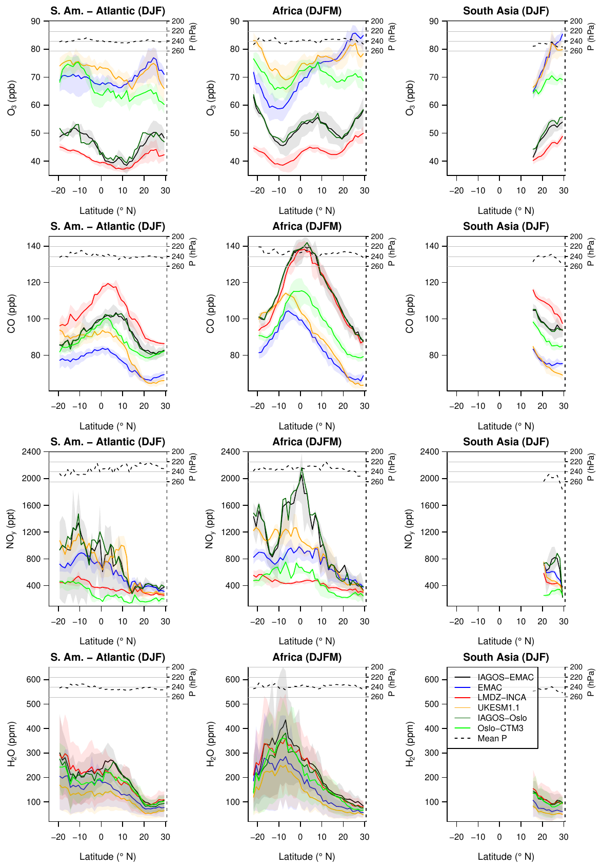
Figure 11Zonal cross sections between 25° S and 30° N from December until February or March. Each row represents a measured variable, and each column (from left to right) represents the corresponding region: South America–Atlantic Ocean, Africa, and South Asia. The uncertainties shown here correspond to the spatial variability, defined as the interval between quartiles 1 and 3. The solid black and dark-green lines correspond to IAGOS–EMAC and IAGOS–Oslo, respectively. For further visibility, the observational variability is shown only for the IAGOS–EMAC profiles. The blue, red, orange, and green lines correspond to the reference simulation from EMAC, LMDZ–INCA, UKESM1.1, and OsloCTM3, respectively. The dashed line at the top of each panel shows the mean pressure derived from IAGOS–EMAC; its values are reported on the right axis.
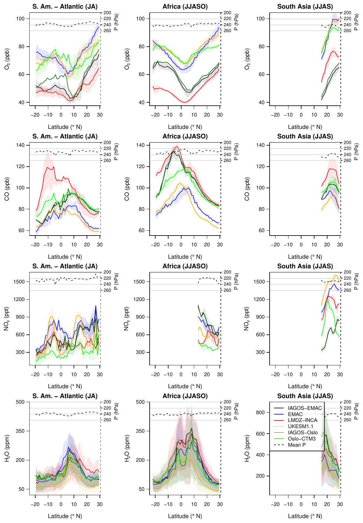
Figure 12Same as Fig. 11 but for July–August, June–October, and June–September (from left to right). Please note the different scale for water vapour in the right column.
Most of the observed features have been investigated in Cohen et al. (2023), such as the impacts of wet and dry seasons, linked to shifts in the ITCZ. In the two western regions (South America and Africa), where the zonal cross sections cover most of the tropical latitudes, the wet season is characterized by a co-located maximum in water vapour and a minimum in ozone, both linked to the intense convection of humid surface air. The latter is rather rich in fresh pollutants and becomes enriched in NOx emitted by lightning during convective uplift. In the upper branch of both Hadley cells, ozone is produced by photochemistry during its poleward transport.
Above Africa, the seasons with the northernmost and the southernmost ITCZ (June–October and December–March, respectively) are particularly visible in the IAGOS observations. During the meridional transport in the upper branch of the strongest Hadley cell, CO accumulates in the areas where zonal wind shear is greater (Sauvage et al., 2007; Lannuque et al., 2021), visible in December–March for NOy, reaching a maximum at approximately 10° from the ITCZ. Using a method based on the FLEXPART Lagrangian dispersion model (SOFT-IO; Sauvage et al., 2017), Lannuque et al. (2021) found that these CO peaks originated from intense biomass burning in the dry season. A sensitivity test regarding biomass burning with the LMDZ–INCA model (Cohen et al., 2023) found similar conclusions. In the monsoon season (June–October), both studies agree on a major biomass burning contribution to the southward shift in the peak of CO. Finally, the Asian summer monsoon (right panels in Fig. 12) is characterized by the warmest and most humid air masses, as expected from the strongest convective system. During this season, the subtropical jet stream and its subsequent stratospheric intrusions are confined to the northern side of the Himalayas (Cristofanelli et al., 2010), thereby ensuring a weak stratospheric influence in this season (Gottschaldt et al., 2018).
The analysis of the modelled local and seasonal features provides interesting information about the representation of the convective systems and their outflows. All of the models capture the location of the peaks in water vapour in the African upper troposphere, irrespective of the season; the maximized water vapour amounts (as well as temperature, not shown) above the Asian summer monsoon (Fig. 12, right column); and the strongest CO peaks above Africa. More precisely, above Africa, in the December–March (June–October) season, the models capture the southward (northward) shift in the ITCZ relatively well, as characterized by an ozone minimum co-located with the water vapour maximum. This agreement among the models and with the observations highlights a realistic representation of the strongest convective systems. It is probably improved by the nudging, by the use of a common surface temperature field based on observations, and by a common (or similar) inventory for biomass burning emissions.
Regarding the effects of convection, the variability between the models can be found in the peaks' intensity of water vapour and CO and in the CO peaks' location. In most cases, water vapour shows a small bias for LMDZ–INCA and OsloCTM3 and a dry bias for EMAC and UKESM1.1. The EMAC dry bias is possibly explained by a cold bias in the UT ( K, not shown) that lowers the saturation vapour pressure and/or the detrainment altitudes. The other models show particularly well-reproduced temperatures, and all of the modelled temperature profiles are well correlated with the observations (not shown).
The location and the width of the CO maximum depend on the model, notably above Africa: it is rather co-located with the ITCZ for the EMAC and UKESM1.1 models, whereas it is shifted 5–10° equatorward for the other models, in agreement with the observations. Concerning June–October, with the same observation dataset, Lannuque et al. (2021) showed a peak in the anthropogenic contribution to upper-tropospheric CO co-located with the ITCZ (as for EMAC and, to a lesser extent, UKESM1.1 and OsloCTM3) and a peak in the biomass burning contribution shifted 10° southward (as for the LMDZ–INCA model). OsloCTM3 seems to show a compromise between the two categories, with a flatter and wider maximum including both the ITCZ position and the observed CO peak. A sensitivity test (Cohen et al., 2023) using the LMDZ–INCA model that reproduces the CO peak during December–March and June–October well (with respect to its location and its magnitude, the latter of which is near 140 ppb) concluded that biomass burning is the main factor influencing the peak intensity, with a contribution reaching 30 and 45 ppb during DJFM and JJASO, respectively, but also with a southward shift in the CO peak during June–October. Thus, the negative CO bias, combined with the absence of the southward shift in the EMAC and UKESM1.1 simulations, is likely to reflect an underestimation of the impact of biomass burning in the tropical UT. As the dry bias in the water vapour peaks in these two models suggests a less intense convection, it implies a weaker Hadley circulation. Consequently, the lower-tropospheric entrainment into convective motions in the ITCZ has a reduced geographical extent and, thus, includes less air from the dry region. This could explain the lack of CO accumulation in the higher tropical latitudes with these two models. Inversely, the LMDZ–INCA model and, to a lesser extent, OsloCTM3 show another peak in CO in July–August above South America at relatively similar latitudes to the peak in Africa, although this is absent from the observation profiles. As it is mainly due to biomass burning for LMDZ–INCA (Cohen et al., 2023) and because LMDZ–INCA and OsloCTM3 show similar behaviours for CO, it suggests that both models overestimate the effects of the intercontinental connection with Africa during this season (with respect to duration and/or intensity) or the impact of local biomass burning emissions.
Contrary to CO, the peaks in NOy observed in December–February (December–March) show an important negative bias in LMDZ–INCA and OsloCTM3, whereas the negative bias is lower with EMAC and UKESM1.1, especially above South America. Concerning the Asian summer monsoon, all of the represented models overestimate ozone and NOy mixing ratios, possibly reflecting an overestimation of the lightning flash rate, as is known for LMDZ–INCA (Hauglustaine et al., 2004); an underestimation of HNO3 uptake; and/or an overestimation of the entrained surface pollutants.
Most of the models tend to overestimate ozone, except for the LMDZ–INCA model that instead shows negative biases. The overestimation of ozone in the tropical UT from UKESM1.1 is consistent with a recent comparison based on ozone partial columns between UM–UKCA and the OMI–MLS satellite observations (Russo et al., 2023) during the 2005–2018 period and in the 450–170 hPa pressure range. The overestimation is representative of the whole tropospheric ozone column in the tropics, and the main factor in the UT is probably an overestimation of the lightning NOx emissions. The LMDZ–INCA model shows particularly low NOx levels, with the lowest (highest) mean values near 18 ppt (195 ppt), whereas the other models have NOx minimum (maximum) levels at 52–91 ppt (278–430 ppt). This first-order statement can be sufficient to explain most of the LMDZ–INCA lower ozone values as well as most of the higher CO values with longer photochemical lifetimes for CO. Each of these two factors favours ozone production efficiency from lightning and aviation. A similar diagnostic applies to HNO3. Although the stronger convection with LMDZ–INCA compared to EMAC theoretically produces more NOx due to a higher lightning activity, it is possible that the LMDZ–INCA model overestimates NOy removal by HNO3 wet scavenging, both with a more efficient conversion of NOx into HNO3 and with further precipitation due to a stronger convection.
Table 5Synthesis of the models' ability to reproduce the main features of their respective IAGOS–DM products, regardless of their mean biases.
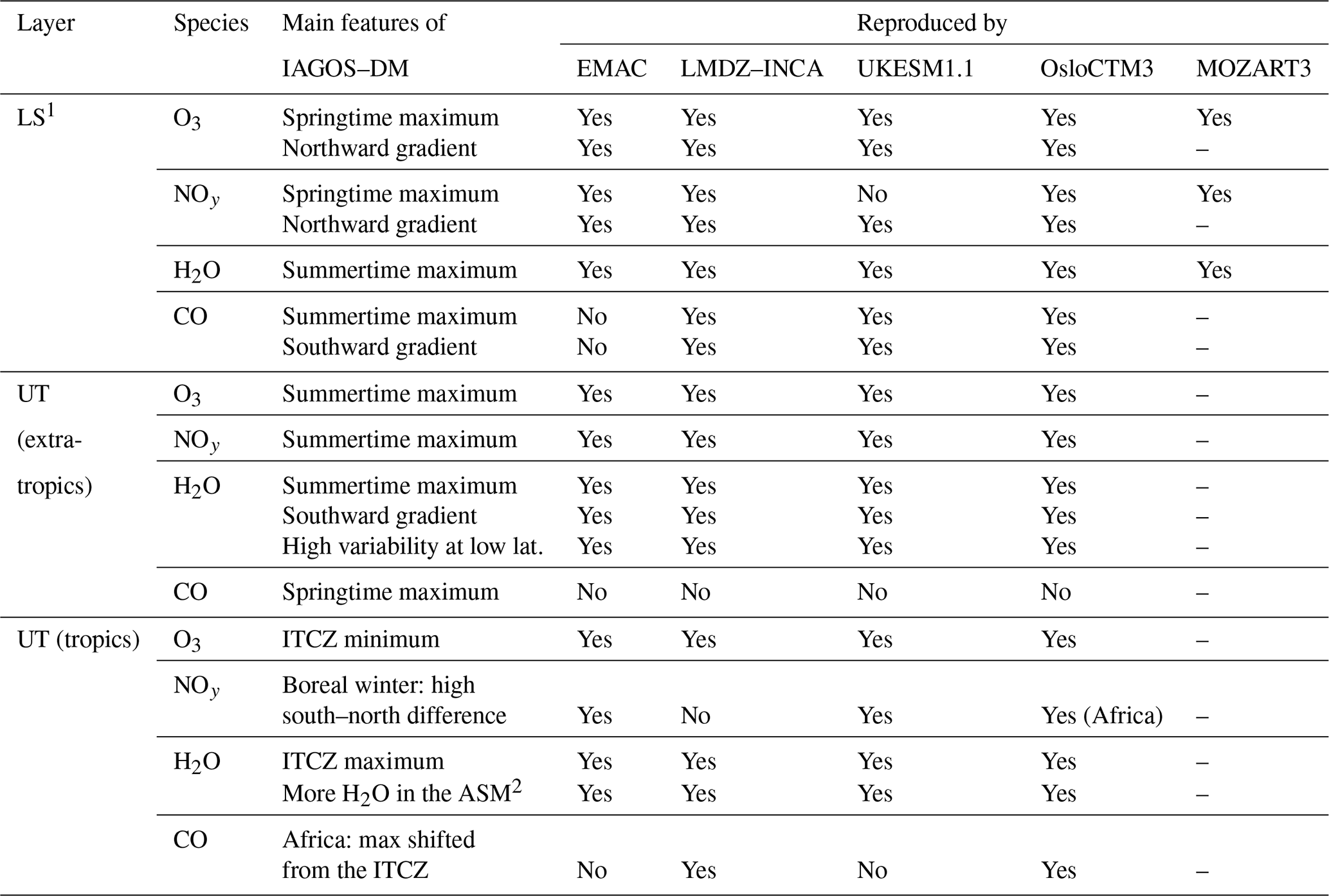
1 Refers to the UTLS for MOZART3 if the feature is also visible in the UTLS with IAGOS–DM. 2 ASM denotes the Asian summer monsoon.
The present study consists of a descriptive evaluation of four global chemistry–climate models (CCMs) and chemistry–transport models (CTMs) against the airborne IAGOS observations. The assessment is based on ozone (O3); carbon monoxide (CO); water vapour (H2O); reactive nitrogen (NOy); and, to a lesser extent, temperature. It relies on airborne measurements during the cruise phases, i.e. in the extratropical upper troposphere–lower stratosphere (UTLS) and in the tropical upper troposphere.
A direct comparison between the model outputs and the IAGOS dataset is made possible via the use of the Interpol-IAGOS software, which projects the IAGOS data onto the model grid with a daily resolution (Cohen et al., 2023). Meanwhile, a daily mask is applied to the model output with respect to the IAGOS sampling. For each grid cell, a weighted monthly average is then derived from both gridded observations and model output. For a given model, the subsequent IAGOS and model products are called the IAGOS–DM–model and model-M, respectively, with the –DM and –M suffixes referring to the distribution onto the model grid and to the IAGOS mask, respectively. This way, each model product is directly comparable to the corresponding IAGOS–DM–model product. In the extra-tropics, the model potential vorticity (PV) is used to treat the upper troposphere (UT) and the lower stratosphere (LS) separately. The assessment is based on the climatologies derived from these products, between 1995 and 2017 for most models. A synthesis of the model skill with respect to reproducing the main observed atmospheric features is proposed in Table 5.
In the northern midlatitudes, the results suggest that most models tend to overestimate the cross-tropopause mixing, which might be linked to an overly diffusive extratropical transition layer. The stratospheric tracers (O3 and, to a lesser extent, NOy) tend to be overestimated in the UT and underestimated in the LS. Concerning the tropospheric tracers (CO and H2O), all of the models systematically underestimate CO in the UT, whereas only two of them systematically underestimate water vapour in this layer. This would be consistent with an underestimation of CO emissions from the CEDS inventory and/or with an overestimation of CO photochemical loss. The geographical distributions are particularly well correlated with observations for ozone in the LS and for water vapour in the UT. The former and the latter suggest a realistic distribution of the impacts from the stratospheric circulation and of the synoptic-scale processes in the troposphere, respectively. The impacts of biomass burning and lightning are harder to reproduce, notably because of the difficulty of parameterizing pyroconvection, lightning, and the washout of soluble species.
The seasonality is generally consistent between models and observations in the UT, the LS, and the non-separated UTLS. Discrepancies are visible with CO in the UT and with ozone in the LS. The former is characterized by a modelled seasonal maximum in winter–spring, contrary to the observed springtime maximum, and an important negative bias in spring, which may suggest an underestimation of CO emissions in winter and spring, as it concerns all of the models. Ozone shows a stronger summertime decrease in the models than in the observations, probably caused by an overestimated influence from the troposphere, particularly during summer and autumn. For each season, the models tend to underestimate the geographical variability in every measured species. One possible consequence of this is an excess in the horizontal homogeneity of the ozone response to aircraft NOx emissions, but it is hard to draw a conclusion on this because the background NOx cannot be compared with the observations in the same way as the other species.
The inter-model variability is particularly noticeable for individual NOy species in both the UT and LS. The median NOx level varies by a factor of up to 3 in the UT and by a factor of up to 7 in the LS. This reflects both different chemical and physical behaviours, such as NOx conversion into HNO3/PAN, HNO3 wet scavenging that removes gaseous NOy from this atmospheric region, or the aerosol uptake of HNO3. This has implications with respect to the model sensitivity to NOx injection in the UTLS from subsonic aviation, as it changes the NOx regime, and with respect to the evaluation of air quality from the models in the subsidence regions, as PAN varies substantially across the models and is rapidly converted into NOx at typical surface temperatures.
The addition of NOx measurements from CARIBIC will allow an evaluation of NOx biases, at least in the most sampled regions. In the longer term, the IAGOS-CORE measurements of NOx will provide the opportunity to also calculate NOx climatologies, with a higher level of sampling. Moreover, particulate matter measurements will provide another variable for the assessment and allow further explanation of the chemical processes related to HNO3. Concerning the models, a more accurate interpretation of the inter-model variability could be provided with additional variables, such as horizontal wind velocities, potential temperature, and inert tropospheric and stratospheric tracers, in order to further isolate the role of dynamics or chemistry in the modelled mixing ratios. In the extra-tropics, the choice of more accurate dynamical coordinates, such as the equivalent latitudes (involving both potential temperature and PV) or the jet-related tropopause (Millán et al., 2024), will probably improve the model assessment, in addition to vertical profiles with tropopause-relative coordinates. Finally, as a complementary part of the current analysis, the models' ability to simulate long-term trends also has to be evaluated.
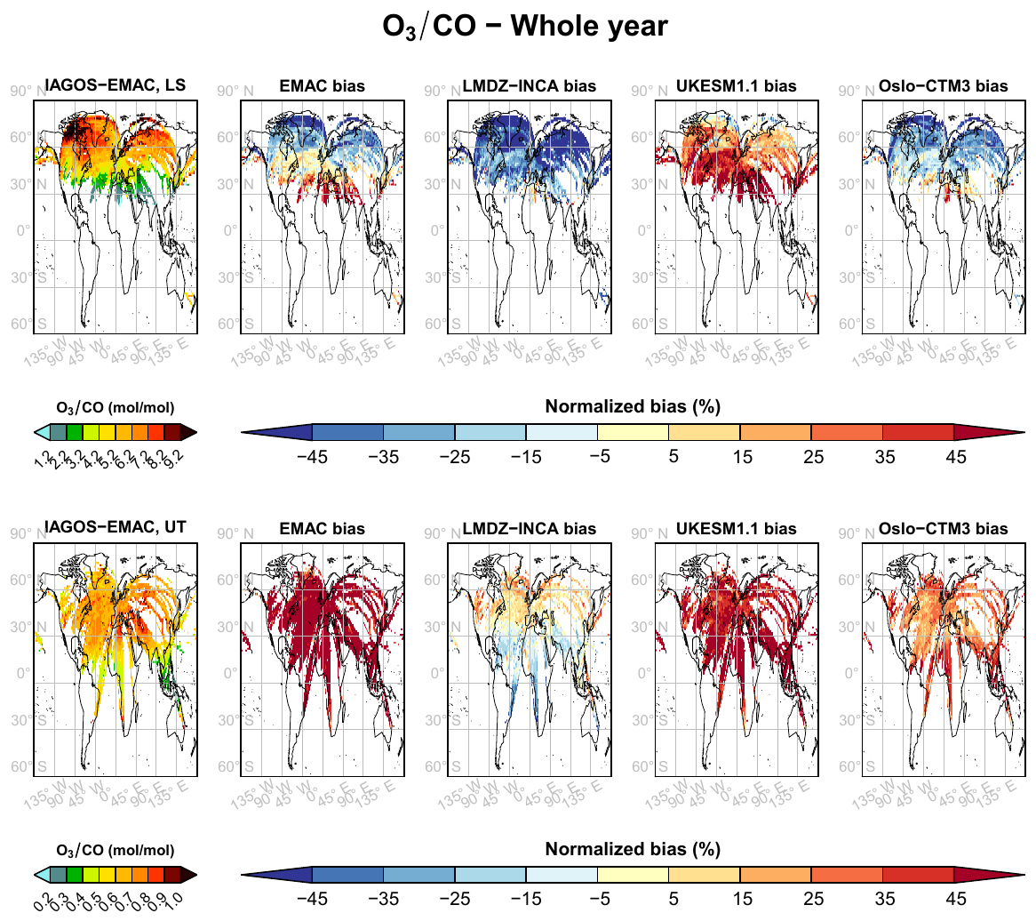
Figure A1Same as Fig. 1 but for the ratio over the period from 2002 to 2017.
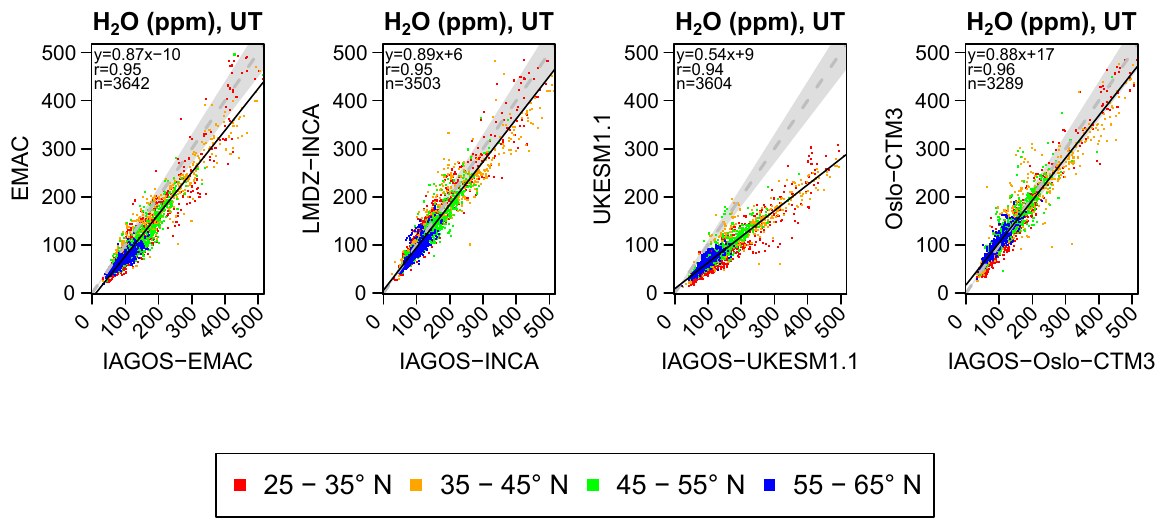
Figure A2Scatterplots comparing the geographical distributions of water vapour in the extratropical UT between the models' output (y axis) and their respective IAGOS products (x axis), in terms of annual means. The colours display a latitude band from subtropical (red) to subpolar (blue) latitudes.
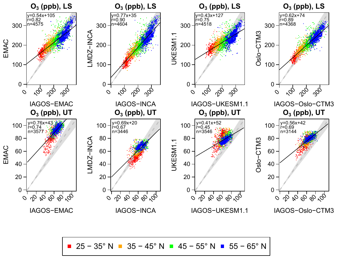
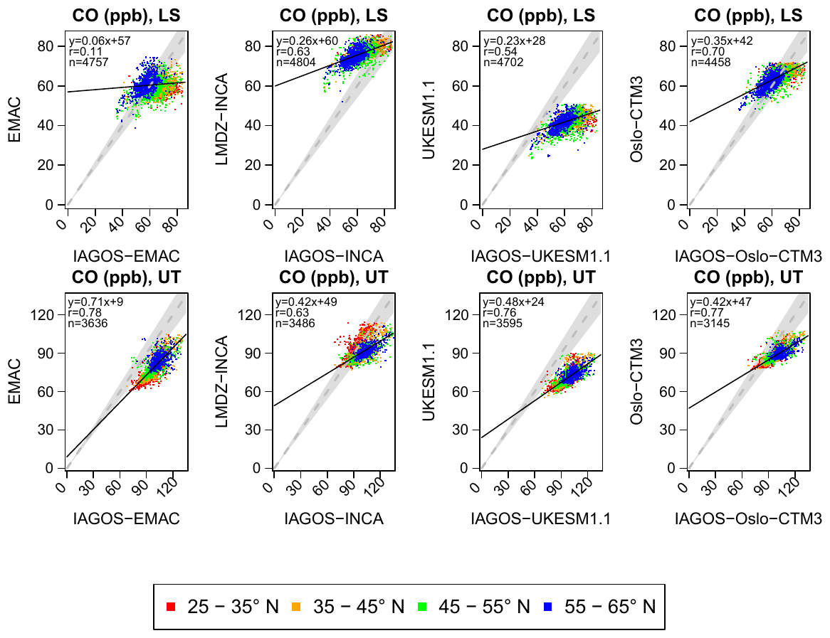
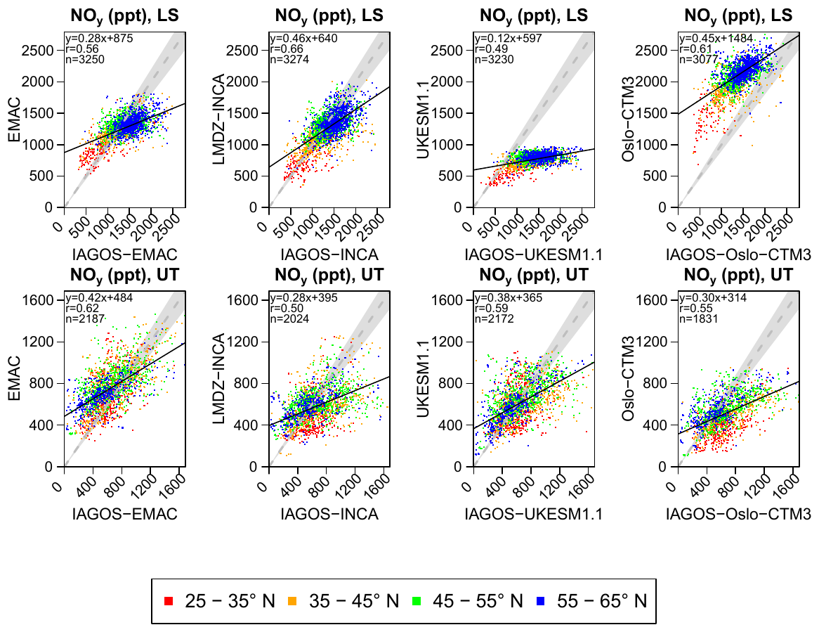
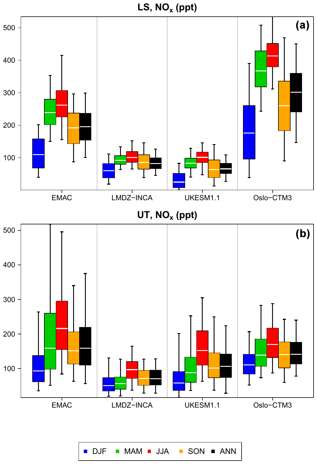
Figure B1Box plots synthesizing the contribution of NOx to the NOy levels shown in Fig. 8 in the LS (a) and the UT (b) for the four model products.
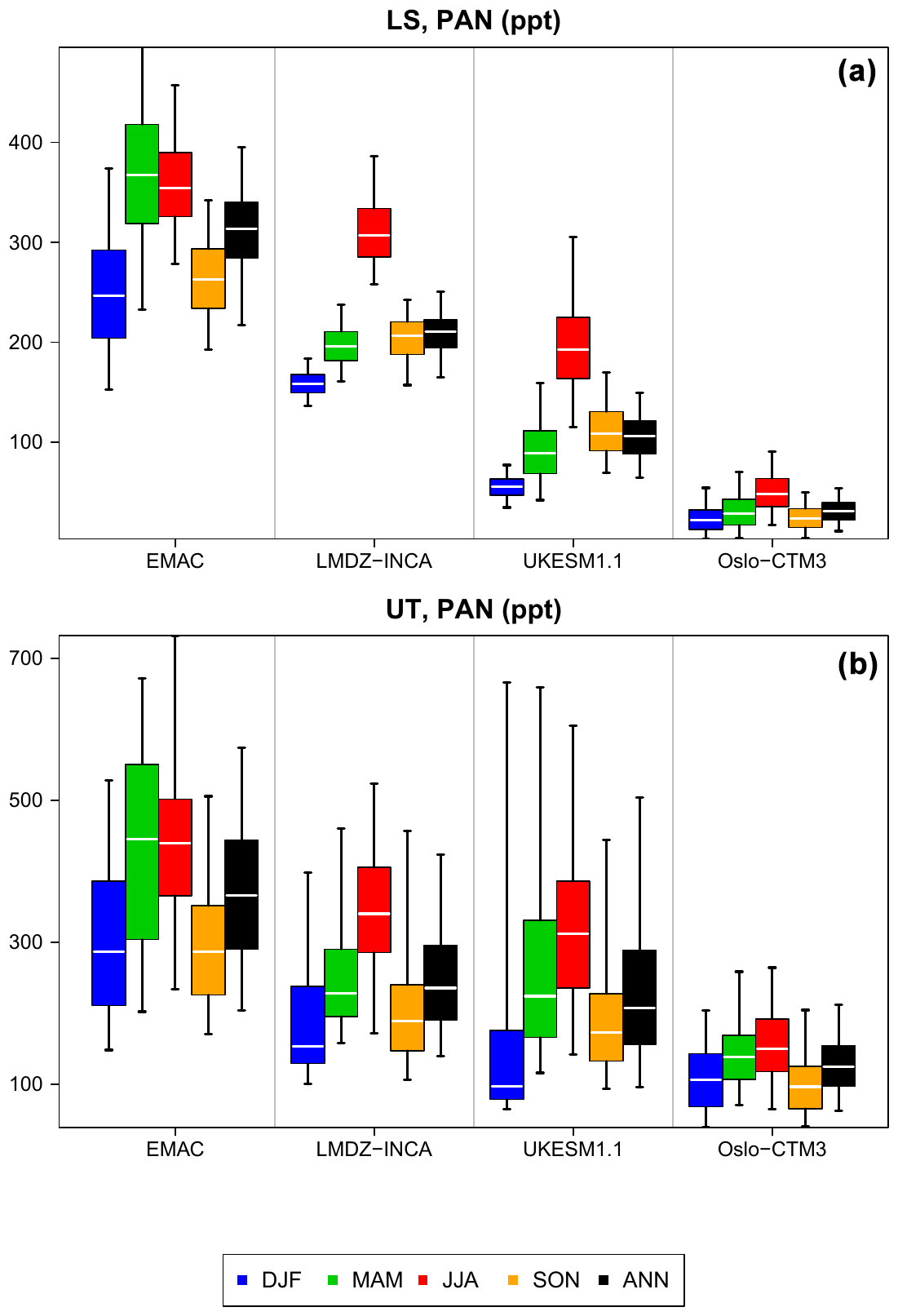
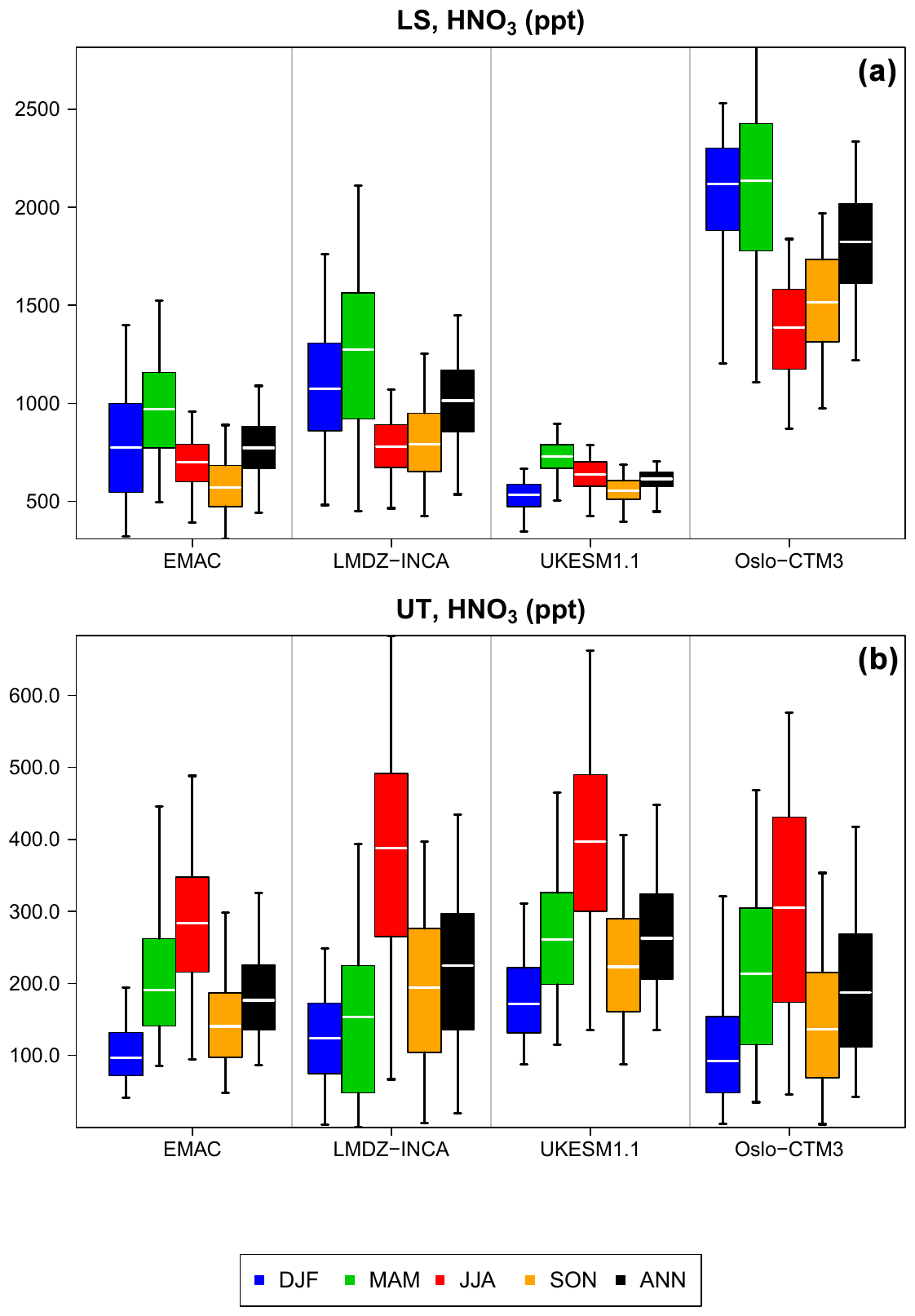
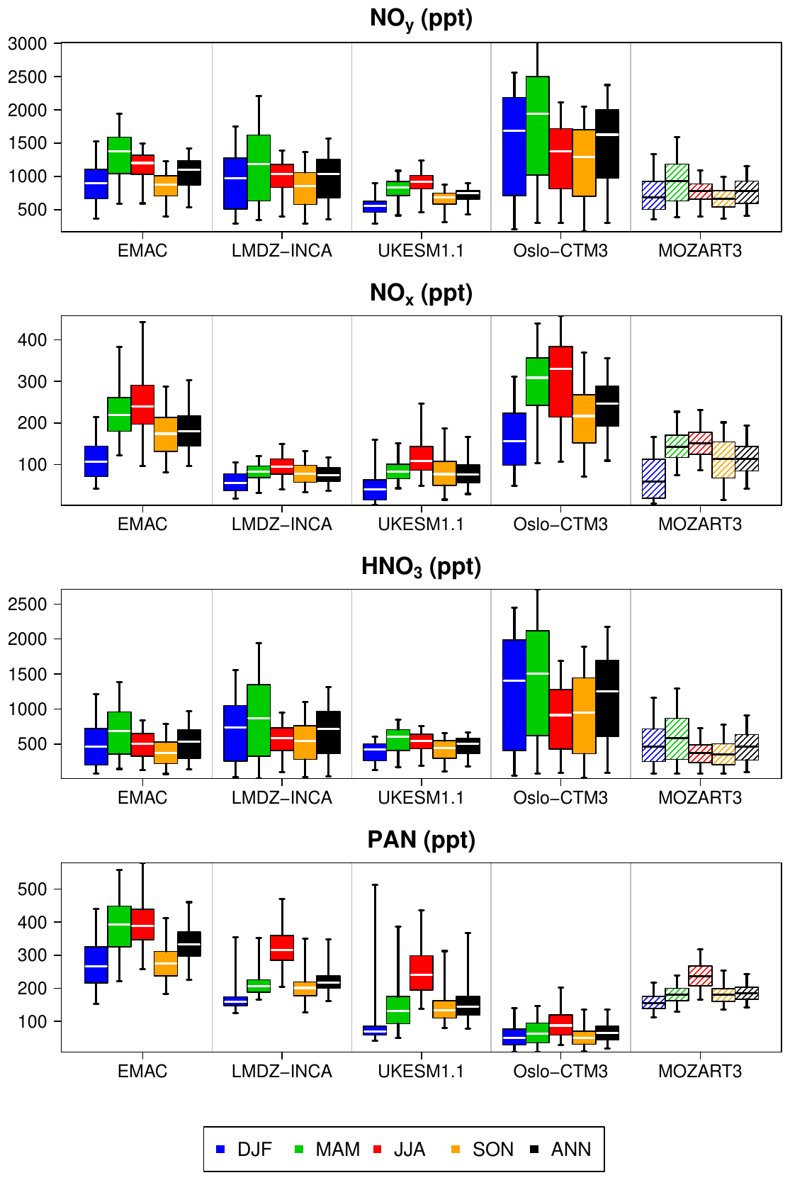
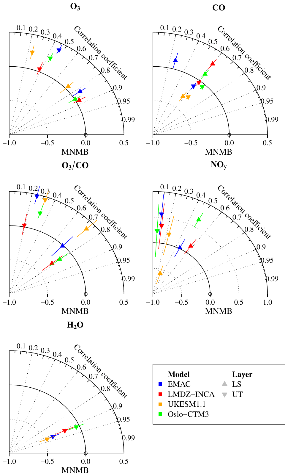
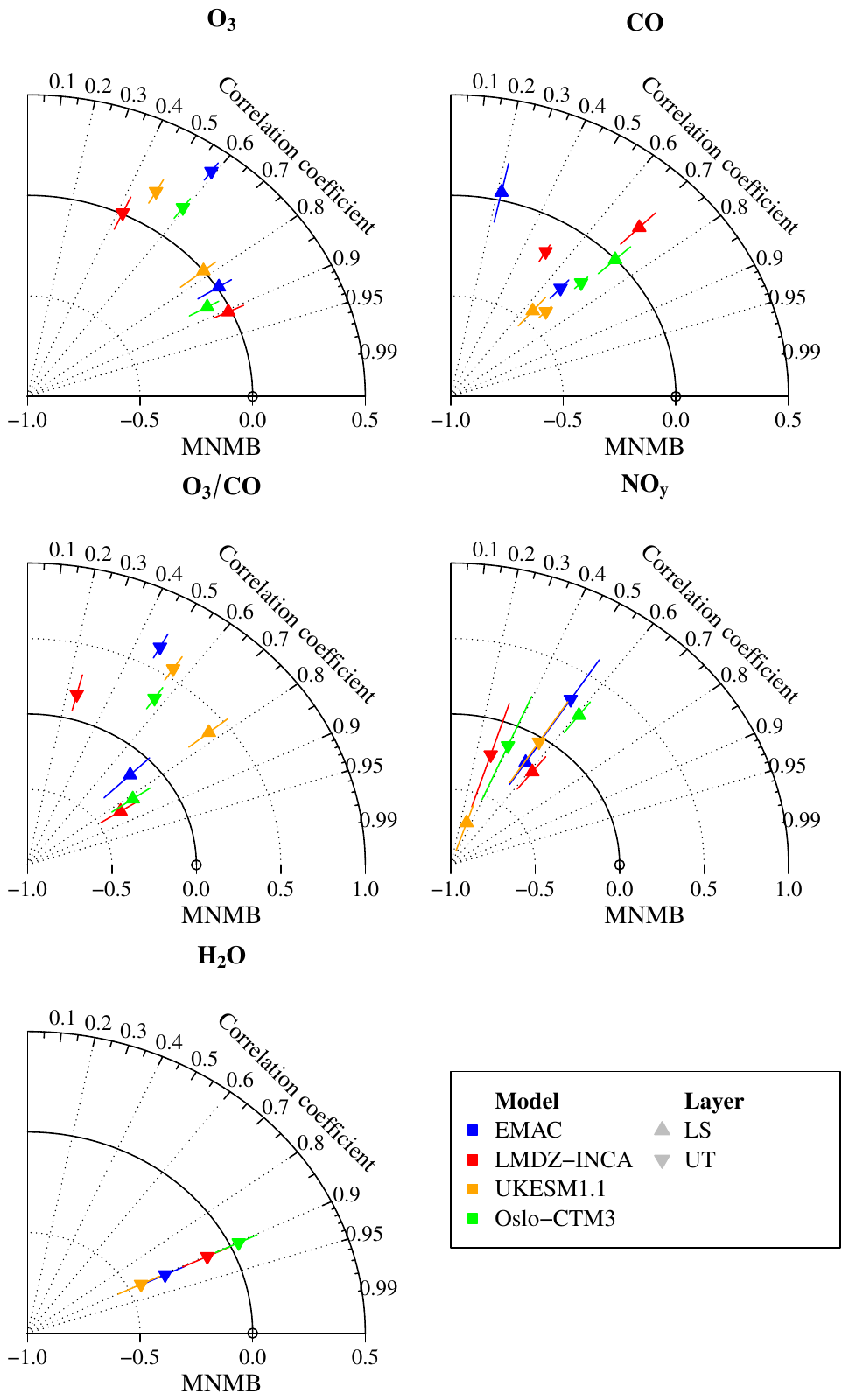
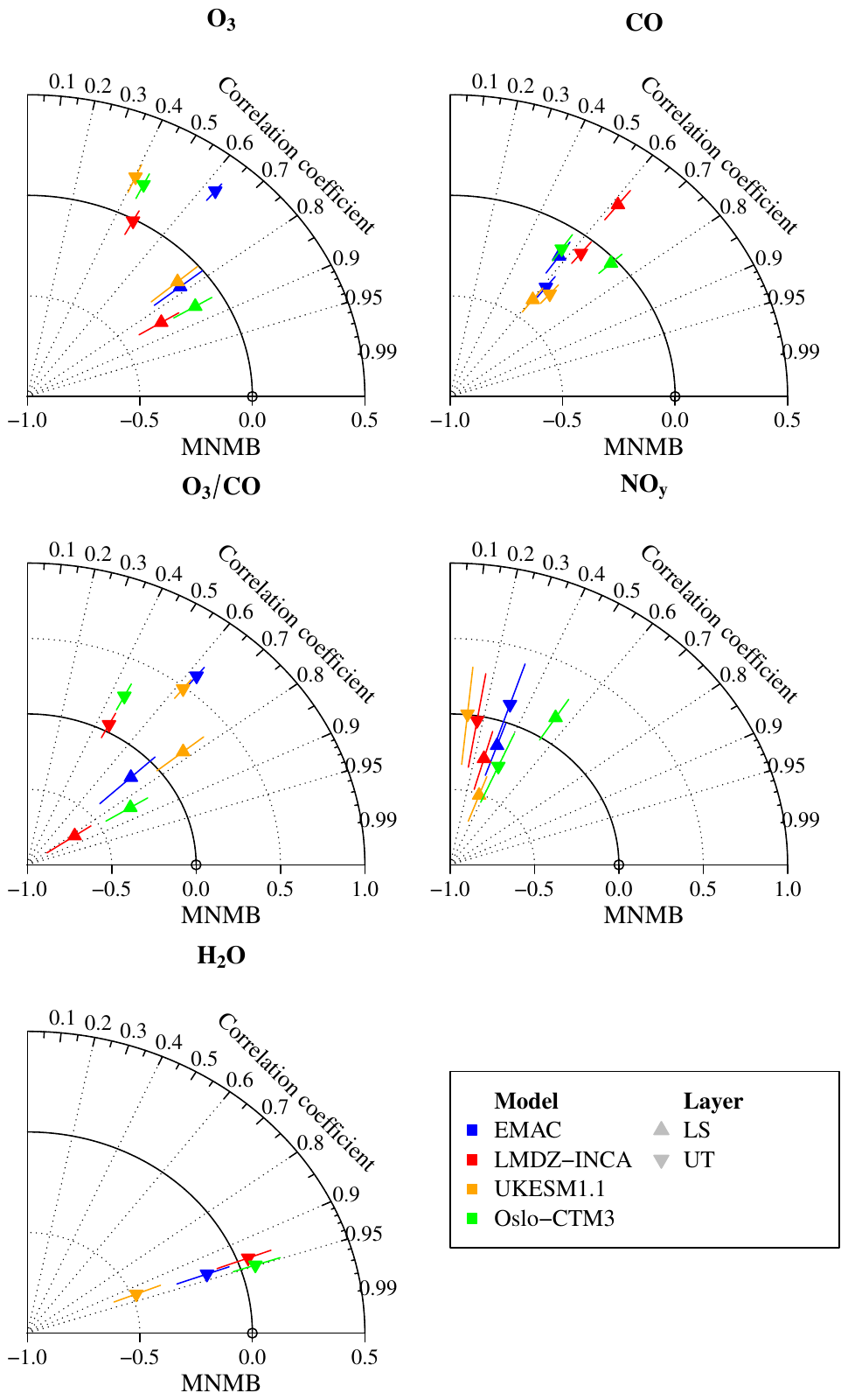
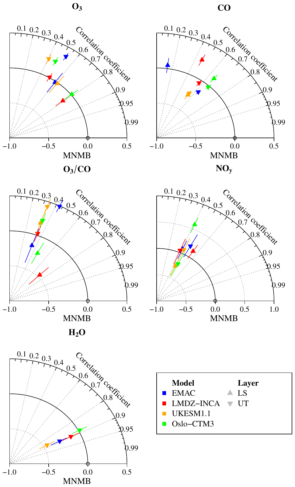
The IAGOS data (IAGOS, 2022) are available from the IAGOS data portal (https://doi.org/10.25326/20); more precisely, the time series data are found at https://doi.org/10.25326/06 (Boulanger et al., 2018). The Interpol-IAGOS software is available at https://doi.org/10.25326/81 (Cohen et al., 2020).
The supplement related to this article is available online at https://doi.org/10.5194/acp-25-5793-2025-supplement.
YC designed the study and further developed the Interpol-IAGOS software. DH designed the modelling protocol shared by the models. The simulation output was provided by SM and RT for EMAC, YC and DH for LMDZ–INCA, AS for MOZART3, MTL for OsloCTM3, and NB for UKESM1.1. The IAGOS data were provided by VT, AP, SR, UB, AZ, and HZ. The paper was written by YC and reviewed, commented upon, edited, and approved by all co-authors.
At least one of the (co-)authors is a member of the editorial board of Atmospheric Chemistry and Physics. The peer-review process was guided by an independent editor, and the authors also have no other competing interests to declare.
Publisher’s note: Copernicus Publications remains neutral with regard to jurisdictional claims made in the text, published maps, institutional affiliations, or any other geographical representation in this paper. While Copernicus Publications makes every effort to include appropriate place names, the final responsibility lies with the authors.
The authors acknowledge strong support from the European Commission; Airbus; and Lufthansa, Air France, Austrian Airlines, Air Namibia, Cathay Pacific, Iberia, and China Airlines, which have carried the IAGOS-CORE equipment and performed maintenance since 1994. In its last 10 years of operation, IAGOS-CORE has been funded by INSU–CNRS (France), Météo-France, Université Paul Sabatier (Toulouse, France), and Research Center Jülich (FZJ, Jülich, Germany). IAGOS has been additionally funded by the EU IAGOS-DS and IAGOS-ERI projects. The IAGOS-CORE database is supported by AERIS. Data are also available on the AERIS website: https://www.aeris-data.fr (last access: 1 November 2022). The simulations were performed using high-performance-computing resources from GENCI (Grand Équipement National de Calcul Intensif) within the framework of the gen2201 project. We also wish to acknowledge our colleagues from the IAGOS teams at FZJ, LAERO, DLR, and KIT for all of the preparation of the IAGOS and CARIBIC data used in this study. Notably, for their contribution to the IAGOS-CORE NOy data, we thank Andreas Volz-Thomas (the former PI) and Karin Thomas (who was involved in the processing of the data).
This research has been funded by the European Union Horizon 2020 Research and Innovation programme, within the framework of the ACACIA (grant agreement no. 875036) project, and by the Direction Générale de l'Aviation Civile (DGAC), under the ClimAviation project. Marianne Tronstad Lund acknowledges funding from the Research Council of Norway (Aviate, grant no. 300718) and resources from the National Infrastructure for High-Performance Computing and Data Storage in Norway (grant no. NN9188K).
This paper was edited by Jianzhong Ma and reviewed by two anonymous referees.
Allen, D., Pickering, K., Duncan, B., and Damon, M.: Impact of lightning NO emissions on North American photochemistry as determined using the Global Modeling Initiative (GMI) model, J. Geophys. Res.-Atmos., 115, https://doi.org/10.1029/2010JD014062, 2010. a, b
Archibald, A. T., O'Connor, F. M., Abraham, N. L., Archer-Nicholls, S., Chipperfield, M. P., Dalvi, M., Folberth, G. A., Dennison, F., Dhomse, S. S., Griffiths, P. T., Hardacre, C., Hewitt, A. J., Hill, R. S., Johnson, C. E., Keeble, J., Köhler, M. O., Morgenstern, O., Mulcahy, J. P., Ordóñez, C., Pope, R. J., Rumbold, S. T., Russo, M. R., Savage, N. H., Sellar, A., Stringer, M., Turnock, S. T., Wild, O., and Zeng, G.: Description and evaluation of the UKCA stratosphere–troposphere chemistry scheme (StratTrop vn 1.0) implemented in UKESM1, Geosci. Model Dev., 13, 1223–1266, https://doi.org/10.5194/gmd-13-1223-2020, 2020. a, b, c
Bellouin, N., Bickel, M., Burkhardt, U., Cohen, Y., Dedoussi, I., Dollner, M., Fuglestvedt, J., Gettelman, A., Gierens, K., Grewe, V., Hahofer, J., Hauglustaine, D., Hendricks, J., Kanji, Z., Kärcher, B., Krämer, M., Lee, D., de Leon, R. R., Li, Y., Lohmann, U., Lund, M. T., Maruhashi, J., Matthes, S., Paoli, R., Penner, J., Petzold, A., Quaas, J., Quadros, F., Righi, M., Samset, B., Skowron, A., Terrenoire, E., Tesche, M., Unterstrasser, S., Voigt, C., and Weinzierl, B.: Assessment of the uncertainty in the effective radiative forcing of aviation: nitrogen oxide emissions, contrail cirrus formation, and aerosol-cloud interactions, in preparation, 2025.
Berntsen, T. K. and Isaksen, I. S. A.: A global three-dimensional chemical transport model for the troposphere: 1. Model description and CO and ozone results, J. Geophys. Res.-Atmos., 102, 21239–21280, https://doi.org/10.1029/97JD01140, 1997. a
Blot, R., Nedelec, P., Boulanger, D., Wolff, P., Sauvage, B., Cousin, J.-M., Athier, G., Zahn, A., Obersteiner, F., Scharffe, D., Petetin, H., Bennouna, Y., Clark, H., and Thouret, V.: Internal consistency of the IAGOS ozone and carbon monoxide measurements for the last 25 years, Atmos. Meas. Tech., 14, 3935–3951, https://doi.org/10.5194/amt-14-3935-2021, 2021. a
Bojinski, S., Verstraete, M., Peterson, T. C., Richter, C., Simmons, A., and Zemp, M.: The Concept of Essential Climate Variables in Support of Climate Research, Applications, and Policy, B. Am. Meteor. Soc., 95, 1431–1443, https://doi.org/10.1175/BAMS-D-13-00047.1, 2014. a
Boulanger, D., Blot, R., Bundke, U., Gerbig, C., Hermann, M., Nédélec, P., Rohs, S., and Ziereis, H.: IAGOS time series, AERIS [data set], https://doi.org/10.25326/06, 2018. a
Brasseur, G. P., Hauglustaine, D. A., Walters, S., Rasch, P. J., Müller, J.-F., Granier, C., and Tie, X.: MOZART, a global chemical transport model for ozone and related tracers, Part 1: model description, J. Geophys. Res.-Atmos., 103, 28265–28289 https://doi.org/10.1029/98JD02397, 1998. a
Brenninkmeijer, C. A. M., Crutzen, P. J., Fischer, H., Güsten, H., Hans, W., Heinrich, G., Heintzenberg, J., Hermann, M., Immelmann, T., Kersting, D., Maiss, M., Nolle, M., Pitscheider, A., Pohlkamp, H., Scharffe, D., Specht, K., and Wiedensohler, A.: CARIBIC–Civil Aircraft for Global Measurement of Trace Gases and Aerosols in the Tropopause Region, J. Atmos. Ocean Tech., 16, 1373–1383, https://doi.org/10.1175/1520-0426(1999)016<1373:CCAFGM>2.0.CO;2, 1999. a
Brenninkmeijer, C. A. M., Crutzen, P., Boumard, F., Dauer, T., Dix, B., Ebinghaus, R., Filippi, D., Fischer, H., Franke, H., Frieβ, U., Heintzenberg, J., Helleis, F., Hermann, M., Kock, H. H., Koeppel, C., Lelieveld, J., Leuenberger, M., Martinsson, B. G., Miemczyk, S., Moret, H. P., Nguyen, H. N., Nyfeler, P., Oram, D., O'Sullivan, D., Penkett, S., Platt, U., Pupek, M., Ramonet, M., Randa, B., Reichelt, M., Rhee, T. S., Rohwer, J., Rosenfeld, K., Scharffe, D., Schlager, H., Schumann, U., Slemr, F., Sprung, D., Stock, P., Thaler, R., Valentino, F., van Velthoven, P., Waibel, A., Wandel, A., Waschitschek, K., Wiedensohler, A., Xueref-Remy, I., Zahn, A., Zech, U., and Ziereis, H.: Civil Aircraft for the regular investigation of the atmosphere based on an instrumented container: The new CARIBIC system, Atmos. Chem. Phys., 7, 4953–4976, https://doi.org/10.5194/acp-7-4953-2007, 2007. a
Brunner, D., Staehelin, J., Rogers, H. L., Köhler, M. O., Pyle, J. A., Hauglustaine, D., Jourdain, L., Berntsen, T. K., Gauss, M., Isaksen, I. S. A., Meijer, E., van Velthoven, P., Pitari, G., Mancini, E., Grewe, G., and Sausen, R.: An evaluation of the performance of chemistry transport models by comparison with research aircraft observations. Part 1: Concepts and overall model performance, Atmos. Chem. Phys., 3, 1609–1631, https://doi.org/10.5194/acp-3-1609-2003, 2003. a
Cecil, D. J., Buechler, D. E., and Blakeslee, R. J.: Gridded lightning climatology from TRMM-LIS and OTD: Dataset description, Atmos. Res., 135-136, 404–414, https://doi.org/10.1016/j.atmosres.2012.06.028, 2014. a
Cohen, Y., Petetin, H., Thouret, V., Marécal, V., Josse, B., Clark, H., Sauvage, B., Fontaine, A., Athier, G., Blot, R., Boulanger, D., Cousin, J.-M., and Nédélec, P.: Climatology and long-term evolution of ozone and carbon monoxide in the upper troposphere–lower stratosphere (UTLS) at northern midlatitudes, as seen by IAGOS from 1995 to 2013, Atmos. Chem. Phys., 18, 5415–5453, https://doi.org/10.5194/acp-18-5415-2018, 2018. a, b, c, d
Cohen, Y., Thouret, V., Marécal, V., and Josse, B.: Interpol-IAGOS software, AERIS [code], https://doi.org/10.25326/81, 2020. a
Cohen, Y., Marécal, V., Josse, B., and Thouret, V.: Interpol-IAGOS: a new method for assessing long-term chemistry–climate simulations in the UTLS based on IAGOS data, and its application to the MOCAGE CCMI REF-C1SD simulation, Geosci. Model Dev., 14, 2659–2689, https://doi.org/10.5194/gmd-14-2659-2021, 2021. a, b, c, d
Cohen, Y., Hauglustaine, D., Sauvage, B., Rohs, S., Konjari, P., Bundke, U., Petzold, A., Thouret, V., Zahn, A., and Ziereis, H.: Evaluation of modelled climatologies of O3, CO, water vapour and NOy in the upper troposphere–lower stratosphere using regular in situ observations by passenger aircraft, Atmos. Chem. Phys., 23, 14973–15009, https://doi.org/10.5194/acp-23-14973-2023, 2023. a, b, c, d, e, f, g, h, i, j, k, l, m, n, o, p
Cohen, Y., Hauglustaine, D., Dedoussi, I., Lund, M., Matthes, S., Righi, M., Quadros, F., Skowron, A., Staniaszek, Z., and Thor, R.: Impact of aviation NOx and aerosol emissions on atmospheric composition and climate: results from a model intercomparison, in preparation, 2025.
Cooper, O. R., Eckhardt, S., Crawford, J. H., Brown, C. C., Cohen, R. C., Bertram, T. H., Wooldridge, P., Perring, A., Brune, W. H., Ren, X., Brunner, D., and Baughcum, S. L.: Summertime buildup and decay of lightning NOx and aged thunderstorm outflow above North America, J. Geophys. Res.-Atmos., 114, D01101, https://doi.org/10.1029/2008JD010293, 2009. a
Cristofanelli, P., Bracci, A., Sprenger, M., Marinoni, A., Bonafè, U., Calzolari, F., Duchi, R., Laj, P., Pichon, J. M., Roccato, F., Venzac, H., Vuillermoz, E., and Bonasoni, P.: Tropospheric ozone variations at the Nepal Climate Observatory-Pyramid (Himalayas, 5079 m a.s.l.) and influence of deep stratospheric intrusion events, Atmos. Chem. Phys., 10, 6537–6549, https://doi.org/10.5194/acp-10-6537-2010, 2010. a
David, L. M., Ravishankara, A., Brewer, J. F., Sauvage, B., Thouret, V., Venkataramani, S., and Sinha, V.: Tropospheric ozone over the Indian subcontinent from 2000 to 2015: Data set and simulation using GEOS-Chem chemical transport model, Atmos. Environ., 219, 117039, https://doi.org/10.1016/j.atmosenv.2019.117039, 2019. a
de F. Forster, P. M. and Shine, K. P.: Radiative forcing and temperature trends from stratospheric ozone changes, J. Geophys. Res.-Atmos., 102, 10841–10855, https://doi.org/10.1029/96JD03510, 1997. a
Deckert, R., Jöckel, P., Grewe, V., Gottschaldt, K.-D., and Hoor, P.: A quasi chemistry-transport model mode for EMAC, Geosci. Model Dev., 4, 195–206, https://doi.org/10.5194/gmd-4-195-2011, 2011. a
Diallo, M., Ern, M., and Ploeger, F.: The advective Brewer–Dobson circulation in the ERA5 reanalysis: climatology, variability, and trends, Atmos. Chem. Phys., 21, 7515–7544, https://doi.org/10.5194/acp-21-7515-2021, 2021. a
Dietmüller, S., Jöckel, P., Tost, H., Kunze, M., Gellhorn, C., Brinkop, S., Frömming, C., Ponater, M., Steil, B., Lauer, A., and Hendricks, J.: A new radiation infrastructure for the Modular Earth Submodel System (MESSy, based on version 2.51), Geosci. Model Dev., 9, 2209–2222, https://doi.org/10.5194/gmd-9-2209-2016, 2016. a
Dyroff, C., Zahn, A., Christner, E., Forbes, R., Tompkins, A. M., and van Velthoven, P. F. J.: Comparison of ECMWF analysis and forecast humidity data with CARIBIC upper troposphere and lower stratosphere observations, Q. J. Roy. Meteor. Soc., 141, 833–844, https://doi.org/10.1002/qj.2400, 2015. a
Eyring, V., Lamarque, J.-F., Hess, P., Arfeuille, F., Bowman, K., Chipperfield, M. P., Duncan, B., Fiore, A., Gettelman, A., Giorgetta, M. A., Granier, C., Hegglin, M., Kinnison, D., Kunze, M., Langematz, U., Luo, B., Martin, R., Matthes, K., Newman, P. A., Peter, T., Robock, A., Ryerson, T., Saiz-Lopez, A., Salawitch, A., Schultz, M., Shepherd, T. G., Shindell, D., Staehelin, J., Tegtmeier, S., Thomason, L., Tilmes, S., Vernier, J.-P., Waugh, D. W., and Young, P. J.: Overview of IGAC/SPARC Chemistry-Climate Model Initiative (CCMI) Community Simulations in Support of Upcoming Ozone and Climate Assessments, SPARC Newsletter, 48–66, 2013. a
Fadnavis, S., Semeniuk, K., Schultz, M. G., Kiefer, M., Mahajan, A., Pozzoli, L., and Sonbawane, S.: Transport pathways of peroxyacetyl nitrate in the upper troposphere and lower stratosphere from different monsoon systems during the summer monsoon season, Atmos. Chem. Phys., 15, 11477–11499, https://doi.org/10.5194/acp-15-11477-2015, 2015. a
Finney, D. L., Doherty, R. M., Wild, O., Young, P. J., and Butler, A.: Response of lightning NOx emissions and ozone production to climate change: Insights from the Atmospheric Chemistry and Climate Model Intercomparison Project, Geophys. Res. Lett., 43, 5492–5500, https://doi.org/10.1002/2016GL068825, 2016. a
Folberth, G. A., Hauglustaine, D. A., Lathière, J., and Brocheton, F.: Interactive chemistry in the Laboratoire de Météorologie Dynamique general circulation model: model description and impact analysis of biogenic hydrocarbons on tropospheric chemistry, Atmos. Chem. Phys., 6, 2273–2319, https://doi.org/10.5194/acp-6-2273-2006, 2006. a
Gaudel, A., Clark, H., Thouret, V., Jones, L., Inness, A., Flemming, J., Stein, O., Huijnen, V., Eskes, H., Nédélec, P., and Boulanger, D.: On the use of MOZAIC-IAGOS data to assess the ability of the MACC reanalysis to reproduce the distribution of ozone and CO in the UTLS over Europe, Tellus B, 67, 27955, https://doi.org/10.3402/tellusb.v67.27955, 2015. a
Gettelman, A., Hegglin, M. I., Son, S.-W., Kim, J., Fujiwara, M., Birner, T., Kremser, S., Rex, M., Añel, J. A., Akiyoshi, H., Austin, J., Bekki, S., Braesike, P., Brühl, C., Butchart, N., Chipperfield, M., Dameris, M., Dhomse, S., Garny, H., Hardiman, S. C., Jöckel, P., Kinnison, D. E., Lamarque, J. F., Mancini, E., Marchand, M., Michou, M., Morgenstern, O., Pawson, S., Pitari, G., Plummer, D., Pyle, J. A., Rozanov, E., Scinocca, J., Shepherd, T. G., Shibata, K., Smale, D., Teyssèdre, H., and Tian, W.: Multimodel assessment of the upper troposphere and lower stratosphere: Tropics and global trends, J. Geophys. Res.-Atmos., 115, D00M08, https://doi.org/10.1029/2009JD013638, 2010. a
Gettelman, A., Hoor, P., Pan, L. L., Randel, W. J., Hegglin, M. I., and Birner, T.: The extratropical upper troposphere and lower stratosphere, Rev. Geophys., 49, RG3003, https://doi.org/10.1029/2011RG000355, 2011. a
Giannakopoulos, C., Chipperfield, T., Law, K., and Pyle, J.: Validation and intercomparison of wet and dry deposition schemes using Pb-210 in a global three-dimensional off-line chemical transport model, J. Geophys. Res., 104, 23761–23784, 1999. a
Gidden, M. J., Riahi, K., Smith, S. J., Fujimori, S., Luderer, G., Kriegler, E., van Vuuren, D. P., van den Berg, M., Feng, L., Klein, D., Calvin, K., Doelman, J. C., Frank, S., Fricko, O., Harmsen, M., Hasegawa, T., Havlik, P., Hilaire, J., Hoesly, R., Horing, J., Popp, A., Stehfest, E., and Takahashi, K.: Global emissions pathways under different socioeconomic scenarios for use in CMIP6: a dataset of harmonized emissions trajectories through the end of the century, Geosci. Model Dev., 12, 1443–1475, https://doi.org/10.5194/gmd-12-1443-2019, 2019. a
Gottschaldt, K.-D., Schlager, H., Baumann, R., Cai, D. S., Eyring, V., Graf, P., Grewe, V., Jöckel, P., Jurkat-Witschas, T., Voigt, C., Zahn, A., and Ziereis, H.: Dynamics and composition of the Asian summer monsoon anticyclone, Atmos. Chem. Phys., 18, 5655–5675, https://doi.org/10.5194/acp-18-5655-2018, 2018. a, b
Granier, C., Lamarque, J.-F., Mieville, A., Muller, J.-F., Olivier, J., Orlando, J., Peters, J., Petron, G., Tyndall, G., and Wallens, S.: POET, a database of surface emissions of ozone precursors, http://www.aero.jussieu.fr/projet/ACCENT/POET.php (last access: 12 May 2022), 2005. a
Grewe, V., Brunner, D., Dameris, M., Grenfell, J., Hein, R., Shindell, D., and Staehelin, J.: Origin and variability of upper tropospheric nitrogen oxides and ozone at northern mid-latitudes, Atmos. Environ., 35, 3421–3433, https://doi.org/10.1016/S1352-2310(01)00134-0, 2001. a
Grooß, J.-U. and Russell III, J. M.: Technical note: A stratospheric climatology for O3, H2O, CH4, NOx, HCl and HF derived from HALOE measurements, Atmos. Chem. Phys., 5, 2797–2807, https://doi.org/10.5194/acp-5-2797-2005, 2005. a
Grooß, J.-U., Brühl, C., and Peter, T.: Impact of aircraft emissions on tropospheric and stratospheric ozone. Part I: chemistry and 2-D model results, Atmos. Environ., 32, 3173–3184, https://doi.org/10.1016/S1352-2310(98)00016-8, 1998. a
Guth, J., Josse, B., Marécal, V., Joly, M., and Hamer, P.: First implementation of secondary inorganic aerosols in the MOCAGE version R2.15.0 chemistry transport model, Geosci. Model Dev., 9, 137–160, https://doi.org/10.5194/gmd-9-137-2016, 2016. a
Hack, J. J.: Parameterization of moist convection in the NCAR community climate model (CCM2), J. Geophys. Res.-Atmos., 99, 5833–5866, https://doi.org/10.1029/93JD03478, 1994. a
Hakim, Z. Q., Archer-Nicholls, S., Beig, G., Folberth, G. A., Sudo, K., Abraham, N. L., Ghude, S., Henze, D. K., and Archibald, A. T.: Evaluation of tropospheric ozone and ozone precursors in simulations from the HTAPII and CCMI model intercomparisons – a focus on the Indian subcontinent, Atmos. Chem. Phys., 19, 6437–6458, https://doi.org/10.5194/acp-19-6437-2019, 2019. a
Hauglustaine, D. A., Hourdin, F., Jourdain, L., Filiberti, M.-A., Walters, S., Lamarque, J.-F., and Holland, E. A.: Interactive chemistry in the Laboratoire de Météorologie Dynamique general circulation model: Description and background tropospheric chemistry evaluation, J. Geophys. Res.-Atmos., 109, https://doi.org/10.1029/2003JD003957, 2004. a, b, c
Hauglustaine, D. A., Balkanski, Y., and Schulz, M.: A global model simulation of present and future nitrate aerosols and their direct radiative forcing of climate, Atmos. Chem. Phys., 14, 11031–11063, https://doi.org/10.5194/acp-14-11031-2014, 2014. a
Hegglin, M. I., Gettelman, A., Hoor, P., Krichevsky, R., Manney, G. L., Pan, L. L., Son, S.-W., Stiller, G., Tilmes, S., Walker, K. A., Eyring, V., Shepherd, T. G., Waugh, D., Akiyoshi, H., Añel, J. A., Austin, J., Baumgaertner, A., Bekki, S., Braesicke, P., Brühl, C., Butchart, N., Chipperfield, M., Dameris, M., Dhomse, S., Frith, S., Garny, H., Hardiman, S. C., Jöckel, P., Kinnison, D. E., Lamarque, J.-F., Mancini, E., Michou, M., Morgenstern, O., Nakamura, T., Olivié, D., Pawson, S., Pitari, G., Plummer, D. A., Pyle, J. A., Rozanov, E., Scinocca, J. F., Shibata, K., Smale, D., Teyssèdre, H., Tian, W., and Yamashita, Y.: Multimodel assessment of the upper troposphere and lower stratosphere: Extratropics, J. Geophys. Res.-Atmos., 115, https://doi.org/10.1029/2010JD013884, 2010. a, b
Helten, M., Smit, H. G. J., Sträter, W., Kley, D., Nédélec, P., Zöger, M., and Busen, R.: Calibration and performance of automatic compact instrumentation for the measurement of relative humidity from passenger aircraft, J. Geophys. Res.-Atmos., 103, 25643–25652, https://doi.org/10.1029/98JD00536, 1998. a
Hesstvedt, E., Hov, O., and Isaksen, I. S. A.: Quasi-steady-state approximations in air pollution modeling: Comparison of two numerical schemes for oxidant prediction, Int. J. Chem. Kinet., 10, 971–994, https://doi.org/10.1002/kin.550100907, 1978. a
Hodnebrog, Ø., Berntsen, T. K., Dessens, O., Gauss, M., Grewe, V., Isaksen, I. S. A., Koffi, B., Myhre, G., Olivié, D., Prather, M. J., Pyle, J. A., Stordal, F., Szopa, S., Tang, Q., van Velthoven, P., Williams, J. E., and Ødemark, K.: Future impact of non-land based traffic emissions on atmospheric ozone and OH – an optimistic scenario and a possible mitigation strategy, Atmos. Chem. Phys., 11, 11293–11317, https://doi.org/10.5194/acp-11-11293-2011, 2011. a
Hodnebrog, Ø., Berntsen, T. K., Dessens, O., Gauss, M., Grewe, V., Isaksen, I. S. A., Koffi, B., Myhre, G., Olivié, D., Prather, M. J., Stordal, F., Szopa, S., Tang, Q., van Velthoven, P., and Williams, J. E.: Future impact of traffic emissions on atmospheric ozone and OH based on two scenarios, Atmos. Chem. Phys., 12, 12211–12225, https://doi.org/10.5194/acp-12-12211-2012, 2012. a
Hoesly, R. M., Smith, S. J., Feng, L., Klimont, Z., Janssens-Maenhout, G., Pitkanen, T., Seibert, J. J., Vu, L., Andres, R. J., Bolt, R. M., Bond, T. C., Dawidowski, L., Kholod, N., Kurokawa, J.-I., Li, M., Liu, L., Lu, Z., Moura, M. C. P., O'Rourke, P. R., and Zhang, Q.: Historical (1750–2014) anthropogenic emissions of reactive gases and aerosols from the Community Emissions Data System (CEDS), Geosci. Model Dev., 11, 369–408, https://doi.org/10.5194/gmd-11-369-2018, 2018. a
Holtslag, A. and Boville, B. A.: Local versus nonlocal boundary-layer diffusion in a global climate model, J. Climate, 6, 1825–1842, https://doi.org/10.1175/1520-0442(1993)006<1825:LVNBLD>2.0.CO;2, 1993. a
Holtslag, A. A. M., De Bruijn, E. I. F., and Pan, H.-L.: A high resolution air mass transformation model for short-range weather forecasting, Mon. Weather Rev., 118, 1561–1575, https://doi.org/10.1175/1520-0493(1990)118<1561:AHRAMT>2.0.CO;2, 1990. a
Hoor, P., Borken-Kleefeld, J., Caro, D., Dessens, O., Endresen, O., Gauss, M., Grewe, V., Hauglustaine, D., Isaksen, I. S. A., Jöckel, P., Lelieveld, J., Myhre, G., Meijer, E., Olivie, D., Prather, M., Schnadt Poberaj, C., Shine, K. P., Staehelin, J., Tang, Q., van Aardenne, J., van Velthoven, P., and Sausen, R.: The impact of traffic emissions on atmospheric ozone and OH: results from QUANTIFY, Atmos. Chem. Phys., 9, 3113–3136, https://doi.org/10.5194/acp-9-3113-2009, 2009. a, b
Hourdin, F., Musat, I., Bony, S., Braconnot, P., Codron, F., Dufresne, J.-L., Fairhead, L., Filiberti, M.-A., Friedlingstein, P., Grandpeix, J.-Y., Krinner, G., LeVan, P., Li, Z.-X., and Lott, F.: The LMDZ4 general circulation model: climate performance and sensitivity to parametrized physics with emphasis on tropical convection, Clim. Dynam., 27, 787–813, https://doi.org/10.1007/s00382-006-0158-0, 2006. a, b
IAGOS: IAGOS-Core and IAGOS-CARIBIC data, https://doi.org/10.25326/20, 2022. a
Iglesias-Suarez, F., Kinnison, D. E., Rap, A., Maycock, A. C., Wild, O., and Young, P. J.: Key drivers of ozone change and its radiative forcing over the 21st century, Atmos. Chem. Phys., 18, 6121–6139, https://doi.org/10.5194/acp-18-6121-2018, 2018. a
Jöckel, P., Kerkweg, A., Pozzer, A., Sander, R., Tost, H., Riede, H., Baumgaertner, A., Gromov, S., and Kern, B.: Development cycle 2 of the Modular Earth Submodel System (MESSy2), Geosci. Model Dev., 3, 717–752, https://doi.org/10.5194/gmd-3-717-2010, 2010. a
Jöckel, P., Tost, H., Pozzer, A., Kunze, M., Kirner, O., Brenninkmeijer, C. A. M., Brinkop, S., Cai, D. S., Dyroff, C., Eckstein, J., Frank, F., Garny, H., Gottschaldt, K.-D., Graf, P., Grewe, V., Kerkweg, A., Kern, B., Matthes, S., Mertens, M., Meul, S., Neumaier, M., Nützel, M., Oberländer-Hayn, S., Ruhnke, R., Runde, T., Sander, R., Scharffe, D., and Zahn, A.: Earth System Chemistry integrated Modelling (ESCiMo) with the Modular Earth Submodel System (MESSy) version 2.51, Geosci. Model Dev., 9, 1153–1200, https://doi.org/10.5194/gmd-9-1153-2016, 2016. a
Joppe, P., Schneider, J., Kaiser, K., Fischer, H., Hoor, P., Kunkel, D., Lachnitt, H.-C., Marsing, A., Röder, L., Schlager, H., Tomsche, L., Voigt, C., Zahn, A., and Borrmann, S.: The influence of extratropical cross-tropopause mixing on the correlation between ozone and sulfate aerosol in the lowermost stratosphere, Atmos. Chem. Phys., 24, 7499–7522, https://doi.org/10.5194/acp-24-7499-2024, 2024. a
Josse, B., Simon, P., and Peuch, V.-H.: Radon global simulations with the multiscale chemistry and transport model MOCAGE, Tellus B, 56, 339–356, https://doi.org/10.3402/tellusb.v56i4.16448, 2004. a
Jourdain, L. and Hauglustaine, D. A.: The global distribution of lightning NOx simulated on-line in a general circulation model, Phys. Chem. Earth Pt. C, 26, 585–591, https://doi.org/10.1016/S1464-1917(01)00051-4, 2001. a
Kinnison, D. E., Brausser, G. P., Walters, S., Garcia, R. R., Marsh, D. R., Sassi, F., Harvey, V. L., Randall, C. E., Emmons, L., Lamarque, J. F., Hess, P., Orlando, J. J., Tie, X. X., Randel, W., Pan, L. L., Gettelman, A., Granier, C., Diehl, T., Niemeier, U., and Simmons, A. J.: Sensitivity of chemical tracers to meteorological parameters in the MOZART-3 chemical transport model, J. Geophys. Res.-Atmos., 112, D20302, https://doi.org/10.1029/2006JD007879, 2007. a
Krinner, G., Viovy, N., de Noblet-Ducoudré, N., Ogée, J., Polcher, J., Friedlingstein, P., Ciais, P., Sitch, S., and Prentice, I. C.: A dynamic global vegetation model for studies of the coupled atmosphere-biosphere system, Global Biogeochem. Cy., 19, https://doi.org/10.1029/2003GB002199, 2005. a
Lacis, A. A., Wuebbles, D. J., and Logan, J. A.: Radiative forcing of climate by changes in the vertical distribution of ozone, J. Geophys. Res.-Atmos., 95, 9971–9981, https://doi.org/10.1029/JD095iD07p09971, 1990. a
Lamarque, J.-F., Shindell, D. T., Josse, B., Young, P. J., Cionni, I., Eyring, V., Bergmann, D., Cameron-Smith, P., Collins, W. J., Doherty, R., Dalsoren, S., Faluvegi, G., Folberth, G., Ghan, S. J., Horowitz, L. W., Lee, Y. H., MacKenzie, I. A., Nagashima, T., Naik, V., Plummer, D., Righi, M., Rumbold, S. T., Schulz, M., Skeie, R. B., Stevenson, D. S., Strode, S., Sudo, K., Szopa, S., Voulgarakis, A., and Zeng, G.: The Atmospheric Chemistry and Climate Model Intercomparison Project (ACCMIP): overview and description of models, simulations and climate diagnostics, Geosci. Model Dev., 6, 179–206, https://doi.org/10.5194/gmd-6-179-2013, 2013. a
Lannuque, V., Sauvage, B., Barret, B., Clark, H., Athier, G., Boulanger, D., Cammas, J.-P., Cousin, J.-M., Fontaine, A., Le Flochmoën, E., Nédélec, P., Petetin, H., Pfaffenzeller, I., Rohs, S., Smit, H. G. J., Wolff, P., and Thouret, V.: Origins and characterization of CO and O3 in the African upper troposphere, Atmos. Chem. Phys., 21, 14535–14555, https://doi.org/10.5194/acp-21-14535-2021, 2021. a, b, c, d, e
Law, K. S., Plantevin, P.-H., Thouret, V., Marenco, A., Asman, W. A. H., Lawrence, M., Crutzen, P. J., Muller, J.-F., Hauglustaine, D. A., and Kanakidou, M.: Comparison between global chemistry transport model results and Measurement of Ozone and Water Vapor by Airbus In-Service Aircraft (MOZAIC) data, J. Geophys. Res.-Atmos., 105, 1503–1525, https://doi.org/10.1029/1999JD900474, 2000. a
Lee, D., Fahey, D., Skowron, A., Allen, M., Burkhardt, U., Chen, Q., Doherty, S., Freeman, S., Forster, P., Fuglestvedt, J., Gettelman, A., De León, R., Lim, L., Lund, M., Millar, R., Owen, B., Penner, J., Pitari, G., Prather, M., Sausen, R., and Wilcox, L.: The contribution of global aviation to anthropogenic climate forcing for 2000 to 2018, Atmos. Environ., 244, 117834, https://doi.org/10.1016/j.atmosenv.2020.117834, 2021. a
Li, Y., Dhomse, S. S., Chipperfield, M. P., Feng, W., Chrysanthou, A., Xia, Y., and Guo, D.: Effects of reanalysis forcing fields on ozone trends and age of air from a chemical transport model, Atmos. Chem. Phys., 22, 10635–10656, https://doi.org/10.5194/acp-22-10635-2022, 2022. a
Lin, S. J. and Rood, R. B.: A fast flux form semi-Lagrangian transport scheme on the sphere, Mon. Weather Rev., 124, 2046–2070, https://doi.org/10.1175/1520-0493(1996)124<2046:MFFSLT>2.0.CO;2, 1996. a
Liu, Y., Liu, C. X., Wang, H. P., Tie, X. X., Gao, S. T., Kinnison, D., and Brasseur, G.: Atmospheric tracers during the 2003–2004 stratospheric warming event and impact of ozone intrusions in the troposphere, Atmos. Chem. Phys., 9, 2157–2170, https://doi.org/10.5194/acp-9-2157-2009, 2009. a
Livesey, N. J., Logan, J. A., Santee, M. L., Waters, J. W., Doherty, R. M., Read, W. G., Froidevaux, L., and Jiang, J. H.: Interrelated variations of O3, CO and deep convection in the tropical/subtropical upper troposphere observed by the Aura Microwave Limb Sounder (MLS) during 2004–2011, Atmos. Chem. Phys., 13, 579–598, https://doi.org/10.5194/acp-13-579-2013, 2013. a
Lund, M. T., Myhre, G., Haslerud, A. S., Skeie, R. B., Griesfeller, J., Platt, S. M., Kumar, R., Myhre, C. L., and Schulz, M.: Concentrations and radiative forcing of anthropogenic aerosols from 1750 to 2014 simulated with the Oslo CTM3 and CEDS emission inventory, Geosci. Model Dev., 11, 4909–4931, https://doi.org/10.5194/gmd-11-4909-2018, 2018. a, b
Marenco, A., Thouret, V., Nédélec, P., Smit, H., Helten, M., Kley, D., Karsher, F., Simon, P., Law, K., Pyle, J., Poschmann, G., Von Wrede, R., Hume, C., and Cook, T.: Measurement of ozone and water vapour by Airbus in-service aircraft : The MOZAIC airborne programme, an overview, J. Geophys. Res., 103, 25631–25642, https://doi.org/10.1029/98JD00977, 1998. a
Messina, P., Lathière, J., Sindelarova, K., Vuichard, N., Granier, C., Ghattas, J., Cozic, A., and Hauglustaine, D. A.: Global biogenic volatile organic compound emissions in the ORCHIDEE and MEGAN models and sensitivity to key parameters, Atmos. Chem. Phys., 16, 14169–14202, https://doi.org/10.5194/acp-16-14169-2016, 2016. a
Millán, L. F., Hoor, P., Hegglin, M. I., Manney, G. L., Boenisch, H., Jeffery, P., Kunkel, D., Petropavlovskikh, I., Ye, H., Leblanc, T., and Walker, K.: Exploring ozone variability in the upper troposphere and lower stratosphere using dynamical coordinates, Atmos. Chem. Phys., 24, 7927–7959, https://doi.org/10.5194/acp-24-7927-2024, 2024. a
Morgenstern, O., Braesicke, P., O'Connor, F. M., Bushell, A. C., Johnson, C. E., Osprey, S. M., and Pyle, J. A.: Evaluation of the new UKCA climate-composition model – Part 1: The stratosphere, Geosci. Model Dev., 2, 43–57, https://doi.org/10.5194/gmd-2-43-2009, 2009. a
Mulcahy, J. P., Jones, C., Sellar, A., Johnson, B., Boutle, I. A., Jones, A., Andrews, T., Rumbold, S. T., Mollard, J., Bellouin, N., Johnson, C. E., Williams, K. D., Grosvenor, D. P., and McCoy, D. T.: Improved aerosol processes and effective radiative forcing in HadGEM3 and UKESM1, J. Adv. Model. Earth Sy., 10, 2786–2805, https://doi.org/10.1029/2018MS001464, 2018. a
Murray, L. T., Jacob, D. J., Logan, J. A., Hudman, R. C., and Koshak, W. J.: Optimized regional and interannual variability of lightning in a global chemical transport model constrained by LIS/OTD satellite data, J. Geophys. Res.-Atmos., 117, https://doi.org/10.1029/2012JD017934, 2012. a
Müller, J.-F.: Geographical distribution and seasonal variation of surface emissions and deposition velocities of atmospheric trace gases, J. Geophys. Res.-Atmos., 97, 3787–3804, https://doi.org/10.1029/91JD02757, 1992. a
Nedelec, P., Cammas, J.-P., Thouret, V., Athier, G., Cousin, J.-M., Legrand, C., Abonnel, C., Lecoeur, F., Cayez, G., and Marizy, C.: An improved infrared carbon monoxide analyser for routine measurements aboard commercial Airbus aircraft: technical validation and first scientific results of the MOZAIC III programme, Atmos. Chem. Phys., 3, 1551–1564, https://doi.org/10.5194/acp-3-1551-2003, 2003. a
Nédélec, P., Blot, R., Boulanger, D., Athier, G., Cousin, J.-M., Gautron, B., Petzold, A., Volz-Thomas, A., and Thouret, V.: Instrumentation on commercial aircraft for monitoring the atmospheric composition on a global scale: the IAGOS system, technical overview of ozone and carbon monoxide measurements, Tellus B, 67, 27791, https://doi.org/10.3402/tellusb.v67.27791, 2015. a
Neis, P., Smit, H. G. J., Krämer, M., Spelten, N., and Petzold, A.: Evaluation of the MOZAIC Capacitive Hygrometer during the airborne field study CIRRUS-III, Atmos. Meas. Tech., 8, 1233–1243, https://doi.org/10.5194/amt-8-1233-2015, 2015a. a
Neis, P., Smit, H. G. J., Rohs, S., Bundke, U., Krämer, M., Spelten, N., Ebert, V., Buchholz, B., Thomas, K., and Petzold, A.: Quality assessment of MOZAIC and IAGOS capacitive hygrometers: insights from airborne field studies, Tellus B, 67, 28320, https://doi.org/10.3402/tellusb.v67.28320, 2015b. a
Neu, J. L., Prather, M. J., and Penner, J. E.: Global atmospheric chemistry: Integrating over fractional cloud cover, J. Geophys. Res.-Atmos., 112, https://doi.org/10.1029/2006JD008007, 2007. a
Nussbaumer, C. M., Fischer, H., Lelieveld, J., and Pozzer, A.: What controls ozone sensitivity in the upper tropical troposphere?, Atmos. Chem. Phys., 23, 12651–12669, https://doi.org/10.5194/acp-23-12651-2023, 2023. a
O'Connor, F. M., Johnson, C. E., Morgenstern, O., Abraham, N. L., Braesicke, P., Dalvi, M., Folberth, G. A., Sanderson, M. G., Telford, P. J., Voulgarakis, A., Young, P. J., Zeng, G., Collins, W. J., and Pyle, J. A.: Evaluation of the new UKCA climate-composition model – Part 2: The Troposphere, Geosci. Model Dev., 7, 41–91, https://doi.org/10.5194/gmd-7-41-2014, 2014. a
Orbe, C., Plummer, D. A., Waugh, D. W., Yang, H., Jöckel, P., Kinnison, D. E., Josse, B., Marecal, V., Deushi, M., Abraham, N. L., Archibald, A. T., Chipperfield, M. P., Dhomse, S., Feng, W., and Bekki, S.: Description and Evaluation of the specified-dynamics experiment in the Chemistry-Climate Model Initiative, Atmos. Chem. Phys., 20, 3809–3840, https://doi.org/10.5194/acp-20-3809-2020, 2020. a
Ott, L. E., Pickering, K. E., Stenchikov, G. L., Allen, D. J., DeCaria, A. J., Ridley, B., Lin, R.-F., Lang, S., and Tao, W.-K.: Production of lightning NOx and its vertical distribution calculated from three-dimensional cloud-scale chemical transport model simulations, J. Geophys. Res.-Atmos., 115, https://doi.org/10.1029/2009JD011880, 2010. a, b, c
Pätz, H.-W., Volz-Thomas, A., Hegglin, M. I., Brunner, D., Fischer, H., and Schmidt, U.: In-situ comparison of the NOy instruments flown in MOZAIC and SPURT, Atmos. Chem. Phys., 6, 2401–2410, https://doi.org/10.5194/acp-6-2401-2006, 2006. a
Petzold, A., Thouret, V., Gerbig, C., Zahn, A., Brenninkmeijer, C., Gallagher, M., Hermann, M., Pontaud, M., Ziereis, H., Boulanger, D., Marshall, J., Nédélec, P., Smit, H., Friess, U., Flaud, J.-M., Wahner, A., Cammas, J.-P., and Volz-Thomas, A.: Global-scale atmosphere monitoring by in-service aircraft – current achievements and future prospects of the European Research Infrastructure IAGOS, Tellus B, 67, 28452, https://doi.org/10.3402/tellusb.v67.28452, 2015. a
Petzold, A., Neis, P., Rütimann, M., Rohs, S., Berkes, F., Smit, H. G. J., Krämer, M., Spelten, N., Spichtinger, P., Nédélec, P., and Wahner, A.: Ice-supersaturated air masses in the northern mid-latitudes from regular in situ observations by passenger aircraft: vertical distribution, seasonality and tropospheric fingerprint, Atmos. Chem. Phys., 20, 8157–8179, https://doi.org/10.5194/acp-20-8157-2020, 2020. a, b
Pickering, K. E., Wang, Y. S., Tao, W. K., Price, C., and Müller, J.: Vertical distributions of lightning NOx for use in regional and global chemical transport models, J. Geophys. Res.-Atmos, 103, 31203–31216, https://doi.org/10.1029/98JD02651, 1998. a, b
Pletzer, J., Hauglustaine, D., Cohen, Y., Jöckel, P., and Grewe, V.: The climate impact of hydrogen-powered hypersonic transport, Atmos. Chem. Phys., 22, 14323–14354, https://doi.org/10.5194/acp-22-14323-2022, 2022. a
Ploeger, F., Diallo, M., Charlesworth, E., Konopka, P., Legras, B., Laube, J. C., Grooß, J.-U., Günther, G., Engel, A., and Riese, M.: The stratospheric Brewer–Dobson circulation inferred from age of air in the ERA5 reanalysis, Atmos. Chem. Phys., 21, 8393–8412, https://doi.org/10.5194/acp-21-8393-2021, 2021. a
Prather, M. J.: Numerical advection by conservation of second-order moments, J. Geophys. Res.-Atmos., 91, 6671–6681, https://doi.org/10.1029/JD091iD06p06671, 1986. a
Prather, M. J.: Fast-JX version 6.5, http://www.ess.uci.edu/~prather/fastJX.html (last access: 1 September 2009), 2009. a
Price, C. and Rind, D.: A simple lightning parameterization for calculating global lightning distributions, J. Geophys. Res.-Atmos., 97, 9919–9933, https://doi.org/10.1029/92JD00719, 1992. a, b, c
Price, C., Penner, J., and Prather, M.: NOx from lightning: 1. Global distribution based on lightning physics, J. Geophys. Res.-Atmos., 102, 5929–5941, https://doi.org/10.1029/96JD03504, 1997. a, b
Riese, M., Ploeger, F., Rap, A., Vogel, B., Konopka, P., Dameris, M., and Forster, P.: Impact of uncertainties in atmospheric mixing on simulated UTLS composition and related radiative effects, J. Geophys. Res., 117, D16305, https://doi.org/10.1029/2012JD017751, 2012. a
Righi, M., Eyring, V., Gottschaldt, K.-D., Klinger, C., Frank, F., Jöckel, P., and Cionni, I.: Quantitative evaluation of ozone and selected climate parameters in a set of EMAC simulations, Geosci. Model Dev., 8, 733–768, https://doi.org/10.5194/gmd-8-733-2015, 2015. a
Roeckner, E., Brokopf, R., Esch, M., Giorgetta, M., Hagemann, S., Kornblueh, L., Manzini, E., Schlese, U., and Schulzweida, U.: Sensitivity of Simulated Climate to Horizontal and Vertical Resolution in the ECHAM5 Atmosphere Model, J. Climate, 19, 3771–3791, https://doi.org/10.1175/JCLI3824.1, 2006. a
Rolf, C., Rohs, S., Smit, H., G. J., Krämer, M., Bozóki, Z., Hofmann, S., Franke, H., Maser, R., Hoor, P., and Petzold, A.: Evaluation of compact hygrometers for continuous airborne measurements, Meteorol. Z., 33, 15–34, https://doi.org/10.1127/metz/2023/1187, 2023. a
Russo, M. R., Kerridge, B. J., Abraham, N. L., Keeble, J., Latter, B. G., Siddans, R., Weber, J., Griffiths, P. T., Pyle, J. A., and Archibald, A. T.: Seasonal, interannual and decadal variability of tropospheric ozone in the North Atlantic: comparison of UM-UKCA and remote sensing observations for 2005–2018, Atmos. Chem. Phys., 23, 6169–6196, https://doi.org/10.5194/acp-23-6169-2023, 2023. a
Sander, R., Baumgaertner, A., Cabrera-Perez, D., Frank, F., Gromov, S., Grooß, J.-U., Harder, H., Huijnen, V., Jöckel, P., Karydis, V. A., Niemeyer, K. E., Pozzer, A., Riede, H., Schultz, M. G., Taraborrelli, D., and Tauer, S.: The community atmospheric chemistry box model CAABA/MECCA-4.0, Geosci. Model Dev., 12, 1365–1385, https://doi.org/10.5194/gmd-12-1365-2019, 2019. a
Sander, S. P., Golden, D. M., Kurylo, M. J., Moortgat, G. K., Wine, P. H., Ravishankara, A. R., Kolb, C. E., Molina, M. J., Finlayson-Pitts, B. J., Huie, R. E., Orkin, V. L., Friedl, R. R., and Keller-Rudek, H.: Chemical kinetics and photochemical data for use in atmospheric studies, Evaluation Number 15, JPL Publication 06-2, Jet Propulsion Laboratory, Pasadena, CA, https://jpldataeval.jpl.nasa.gov (last access: 2 June 2025), 2006. a, b
Sauvage, B., Thouret, V., Cammas, J.-P., Brioude, J., Nédélec, P., and Mari, C.: Meridional ozone gradients in the African upper troposphere, Geophys. Res. Lett., 34, L03817, https://doi.org/10.1029/2006GL028542, 2007. a
Sauvage, B., Fontaine, A., Eckhardt, S., Auby, A., Boulanger, D., Petetin, H., Paugam, R., Athier, G., Cousin, J.-M., Darras, S., Nédélec, P., Stohl, A., Turquety, S., Cammas, J.-P., and Thouret, V.: Source attribution using FLEXPART and carbon monoxide emission inventories: SOFT-IO version 1.0, Atmos. Chem. Phys., 17, 15271–15292, https://doi.org/10.5194/acp-17-15271-2017, 2017. a
Scharffe, D., Slemr, F., Brenninkmeijer, C. A. M., and Zahn, A.: Carbon monoxide measurements onboard the CARIBIC passenger aircraft using UV resonance fluorescence, Atmos. Meas. Tech., 5, 1753–1760, https://doi.org/10.5194/amt-5-1753-2012, 2012. a
Sellar, A. A., Jones, C. G., Mulcahy, J. P., Tang, Y., Yool, A., Wiltshire, A., O'Connor, F. M., Stringer, M., Hill, R., Palmieri, J., Woodward, S., de Mora, L., Kuhlbrodt, T., Rumbold, S. T., Kelley, D. I., Ellis, R., Johnson, C. E., Walton, J., Abraham, N. L., Andrews, M. B., Andrews, T., Archibald, A. T., Berthou, S., Burke, E., Blockley, E., Carslaw, K., Dalvi, M., Edwards, J., Folberth, G. A., Gedney, N., Griffiths, P. T., Harper, A. B., Hendry, M. A., Hewitt, A. J., Johnson, B., Jones, A., Jones, C. D., Keeble, J., Liddicoat, S., Morgenstern, O., Parker, R. J., Predoi, V., Robertson, E., Siahaan, A., Smith, R. S., Swaminathan, R., Woodhouse, M. T., Zeng, G., and Zerroukat, M.: UKESM1: Description and Evaluation of the U.K. Earth System Model, J. Adv. Model. Earth Sy., 11, 4513–4558, https://doi.org/10.1029/2019MS001739, 2019. a
Skowron, A., Lee, D. S., and De León, R. R.: Variation of radiative forcings and global warming potentials from regional aviation NOx/emissions, Atmos. Environ., 104, 69–78, https://doi.org/10.1016/j.atmosenv.2014.12.043, 2015. a
Skowron, A., Lee, D. S., De León, R. R., Lim, L. L., and Owen, B.: Greater fuel efficiency is potentially preferable to reducing NOx/emissions for aviation’s climate impacts, Nat. Commun., 12, 564, https://doi.org/10.1038/s41467-020-20771-3, 2021. a
Smit, H. G. J., Rohs, S., Neis, P., Boulanger, D., Krämer, M., Wahner, A., and Petzold, A.: Technical Note: Reanalysis of upper troposphere humidity data from the MOZAIC programme for the period 1994 to 2009, Atmos. Chem. Phys., 14, 13241–13255, https://doi.org/10.5194/acp-14-13241-2014, 2014. a
Søvde, O. A., Prather, M. J., Isaksen, I. S. A., Berntsen, T. K., Stordal, F., Zhu, X., Holmes, C. D., and Hsu, J.: The chemical transport model Oslo CTM3, Geosci. Model Dev., 5, 1441–1469, https://doi.org/10.5194/gmd-5-1441-2012, 2012. a, b, c
Søvde, O. A., Matthes, S., Skowron, A., Iachetti, D., Lim, L., Owen, B., Hodnebrog, Ø., Di Genova, G., Pitari, G., Lee, D. S., Myhre, G., and Isaksen, I. S.: Aircraft emission mitigation by changing route altitude: A multi-model estimate of aircraft NOx emission impact on O3 photochemistry, Atmos. Environ., 95, 468–479, https://doi.org/10.1016/j.atmosenv.2014.06.049, 2014. a, b
Staniaszek, Z., Hauglustaine, D., Cohen, Y., Matthes, S., Skowron, A., Thor, R., and Lund, M. T.: Dependence of future aviation NOx impacts on background conditions, in preparation, 2025.
Stordal, F., Isaksen, I. S. A., and Horntveth, K.: A diabatic circulation two-dimensional model with photochemistry: Simulations of ozone and long-lived tracers with surface sources, J. Geophys. Res.-Atmos., 90, 5757–5776, https://doi.org/10.1029/JD090iD03p05757, 1985. a
Stratmann, G., Ziereis, H., Stock, P., Brenninkmeijer, C., Zahn, A., Rauthe-Schöch, A., Velthoven, P., Schlager, H., and Volz-Thomas, A.: NO and NOy in the upper troposphere: Nine years of CARIBIC measurements onboard a passenger aircraft, Atmos. Environ., 133, 93–111, https://doi.org/10.1016/j.atmosenv.2016.02.035, 2016. a, b, c, d
Terrenoire, E., Hauglustaine, D. A., Cohen, Y., Cozic, A., Valorso, R., Lefèvre, F., and Matthes, S.: Impact of present and future aircraft NOx and aerosol emissions on atmospheric composition and associated direct radiative forcing of climate, Atmos. Chem. Phys., 22, 11987–12023, https://doi.org/10.5194/acp-22-11987-2022, 2022. a, b
Thor, R. N., Mertens, M., Matthes, S., Righi, M., Hendricks, J., Brinkop, S., Graf, P., Grewe, V., Jöckel, P., and Smith, S.: An inconsistency in aviation emissions between CMIP5 and CMIP6 and the implications for short-lived species and their radiative forcing, Geosci. Model Dev., 16, 1459–1466, https://doi.org/10.5194/gmd-16-1459-2023, 2023. a, b
Thouret, V., Marenco, A., Logan, J. A., Nédélec, P., and Grouhel, C.: Comparisons of ozone measurements from the MOZAIC airborne program and the ozone sounding network at eight locations, J. Geophys. Res., 103, 25695–25720, https://doi.org/10.1029/98JD02243, 1998. a
Thouret, V., Cammas, J.-P., Sauvage, B., Athier, G., Zbinden, R., Nédélec, P., Simon, P., and Karcher, F.: Tropopause referenced ozone climatology and inter-annual variability (1994–2003) from the MOZAIC programme, Atmos. Chem. Phys., 6, 1033–1051, https://doi.org/10.5194/acp-6-1033-2006, 2006. a
Tiedtke, M.: A comprehensive mass flux scheme for cumulus parameterization in large-scale models, Mon. Weather Rev., 117, 1779–1800, https://doi.org/10.1175/1520-0493(1989)117<1779:ACMFSF>2.0.CO;2, 1989. a
Tilmes, S., Pan, L. L., Hoor, P., Atlas, E., Avery, M. A., Campos, T., Christensen, L. E., Diskin, G. S., Gao, R.-S., Herman, R. L., Hintsa, E. J., Loewenstein, M., Lopez, J., Paige, M. E., Pittman, J. V., Podolske, J. R., Proffitt, M. R., Sachse, G. W., Schiller, C., Schlager, H., Smith, J., Spelten, N., Webster, C., Weinheimer, A., and Zondlo, M. A.: An aircraft-based upper troposphere lower stratosphere O3, CO, and H2O climatology for the Northern Hemisphere, J. Geophys. Res.-Atmos., 115, D14303, https://doi.org/10.1029/2009JD012731, 2010. a
Tilmes, S., Lamarque, J.-F., Emmons, L. K., Kinnison, D. E., Marsh, D., Garcia, R. R., Smith, A. K., Neely, R. R., Conley, A., Vitt, F., Val Martin, M., Tanimoto, H., Simpson, I., Blake, D. R., and Blake, N.: Representation of the Community Earth System Model (CESM1) CAM4-chem within the Chemistry-Climate Model Initiative (CCMI), Geosci. Model Dev., 9, 1853–1890, https://doi.org/10.5194/gmd-9-1853-2016, 2016. a
van Marle, M. J. E., Kloster, S., Magi, B. I., Marlon, J. R., Daniau, A.-L., Field, R. D., Arneth, A., Forrest, M., Hantson, S., Kehrwald, N. M., Knorr, W., Lasslop, G., Li, F., Mangeon, S., Yue, C., Kaiser, J. W., and van der Werf, G. R.: Historic global biomass burning emissions for CMIP6 (BB4CMIP) based on merging satellite observations with proxies and fire models (1750–2015), Geosci. Model Dev., 10, 3329–3357, https://doi.org/10.5194/gmd-10-3329-2017, 2017. a
Volz-Thomas, A., Berg, M., Heil, T., Houben, N., Lerner, A., Petrick, W., Raak, D., and Pätz, H.-W.: Measurements of total odd nitrogen (NOy) aboard MOZAIC in-service aircraft: instrument design, operation and performance, Atmos. Chem. Phys., 5, 583–595, https://doi.org/10.5194/acp-5-583-2005, 2005. a
Walters, D., Baran, A. J., Boutle, I., Brooks, M., Earnshaw, P., Edwards, J., Furtado, K., Hill, P., Lock, A., Manners, J., Morcrette, C., Mulcahy, J., Sanchez, C., Smith, C., Stratton, R., Tennant, W., Tomassini, L., Van Weverberg, K., Vosper, S., Willett, M., Browse, J., Bushell, A., Carslaw, K., Dalvi, M., Essery, R., Gedney, N., Hardiman, S., Johnson, B., Johnson, C., Jones, A., Jones, C., Mann, G., Milton, S., Rumbold, H., Sellar, A., Ujiie, M., Whitall, M., Williams, K., and Zerroukat, M.: The Met Office Unified Model Global Atmosphere 7.0/7.1 and JULES Global Land 7.0 configurations, Geosci. Model Dev., 12, 1909–1963, https://doi.org/10.5194/gmd-12-1909-2019, 2019. a, b
Wuebbles, D. J., Patten, K. O., Wang, D., Youn, D., Martínez-Avilés, M., and Francisco, J. S.: Three-dimensional model evaluation of the Ozone Depletion Potentials for n-propyl bromide, trichloroethylene and perchloroethylene, Atmos. Chem. Phys., 11, 2371–2380, https://doi.org/10.5194/acp-11-2371-2011, 2011. a
Young, P. J., Naik, V., Fiore, A. M., Gaudel, A., Guo, J., Lin, M. Y., Neu, J. L., Parrish, D. D., Rieder, H. E., Schnell, J. L., Tilmes, S., Wild, O., Zhang, L., Ziemke, J. R., Brandt, J., Delcloo, A., Doherty, R. M., Geels, C., Hegglin, M. I., Hu, L., Im, U., Kumar, R., Luhar, A., Murray, L., Plummer, D., Rodriguez, J., Saiz-Lopez, A., Schultz, M. G., Woodhouse, M. T., and Zeng, G.: Tropospheric Ozone Assessment Report: Assessment of global-scale model performance for global and regional ozone distributions, variability, and trends, Elem. Sci. Anth., 6, https://doi.org/10.1525/elementa.265, 2018. a
Zahn, A., Weppner, J., Widmann, H., Schlote-Holubek, K., Burger, B., Kühner, T., and Franke, H.: A fast and precise chemiluminescence ozone detector for eddy flux and airborne application, Atmos. Meas. Tech., 5, 363–375, https://doi.org/10.5194/amt-5-363-2012, 2012. a
Zahn, A., Christner, E., van Velthoven, P. F. J., Rauthe-Schöch, A., and Brenninkmeijer, C. A. M.: Processes controlling water vapor in the upper troposphere/lowermost stratosphere: An analysis of 8 years of monthly measurements by the IAGOS-CARIBIC observatory, J. Geophys. Res.-Atmos., 119, 11505–11525, https://doi.org/10.1002/2014JD021687, 2014. a, b, c, d
Zhang, G. J. and McFarlane, N. A.: Sensitivity of climate simulations to the parameterization of cumulus convection in the Canadian climate centre general circulation model, Atmos.-Ocean, 33, 407–446, https://doi.org/10.1080/07055900.1995.9649539, 1995. a
Ziereis, H., Schlager, H., Schulte, P., van Velthoven, P. F. J., and Slemr, F.: Distributions of NO, NOx, and NOy in the upper troposphere and lower stratosphere between 28° and 61° N during POLINAT 2, J. Geophys. Res.-Atmos., 105, 3653–3664, https://doi.org/10.1029/1999JD900870, 2000. a
- Abstract
- Introduction
- Materials and methodology
- Modelled reactive species compared to IAGOS observational data
- Conclusions
- Appendix A: Geographical distributions
- Appendix B: Individual NOy species
- Appendix C: Seasonal assessment of modelled reactive species in the northern extra-tropics
- Code and data availability
- Author contributions
- Competing interests
- Disclaimer
- Acknowledgements
- Financial support
- Review statement
- References
- Supplement