Sensitivity of climate–chemistry model simulated atmospheric composition to the application of an inverse relationship between NO_x emission and lightning flash frequency

Lightning-produced nitrogen oxides (LNO_x = LNO + LNO₂) are an important source of upper-tropospheric ozone. Typical parameterizations of LNO_x in climate–chemistry models introduce a constant amount of NO_x per flash or per flash type. However, recent satellite-based NO₂ measurements suggest that the production of LNO_x per flash depends on the lightning flash frequency. In this study, we implement a new parameterization of LNO_x production per flash based on the lightning flash frequency in a climate–chemistry model to investigate the upper-limit implications for the chemical composition of the atmosphere. We find that a larger production of LNO_x in weak thunderstorms leads to a larger mixing ratio of NO_x in the lower and middle troposphere, as well as to a lower mixing ratio of NO_x in the upper troposphere. The mixing ratios of O₃, CO, HO_x, HNO₃, and HNO₄ in the troposphere are influenced by the simulated changes in LNO_x. Our findings indicate a larger release of nitrogen oxides from lightning in the lower and middle atmosphere, producing a slightly better agreement with the measurements of tropospheric ozone at a global scale. In turn, we obtain a small decrease in the lifetime of methane and carbon monoxide, ranging between 0.7 % and 3.4 %.

1 Introduction

Nitrogen oxides (NO_x = NO + NO₂) produced by lightning in the upper troposphere (Zeldovich et al., 1947) are about 6 times more efficient in driving ozone production than anthropogenic NO_x emissions, producing about 100 molecules of ozone per molecule of lightning-produced NO_x (LNO_x) (Schumann and Huntrieser, 2007). Thus, LNO_x affects the oxidizing capacity of the atmosphere and the tropospheric budget of carbon monoxide and methane (Wu et al., 2007; Murray et al., 2012; Gordillo-Vázquez et al., 2019).

The global production of LNO_x is between 2 and 8 Tg (N) yr⁻¹, which accounts for approximately 10 % of the global NO_x sources. In the tropics, LNO_x is responsible for around 20 % of the total NO_x production (Schumann and Huntrieser, 2007, and references therein). Moreover, the LNO_x production efficiency (PE) per lightning flash shows a large variability between different regions and thunderstorms (e.g., Pickering et al., 2016; Bucsela et al., 2019; Allen et al., 2019, 2021; Zhang et al., 2022; Pérez-Invernón et al., 2022a). In particular, systematic retrievals of LNO_x from the Ozone Monitoring Instrument (OMI) by Bucsela et al. (2019) and Allen et al. (2019) and from the Sentinel-5P TROPOspheric Monitoring Instrument (TROPOMI) by Allen et al. (2021) reported an inverse relationship between flash rates and LNO_x PE per flash. Bucsela et al. (2021) reported a new evaluation of TROPOMI-based LNO_x PE estimations by using Geostationary Lightning Mapper (GLM) lightning measurements and a new set of atmospheric chemistry simulations to estimate the effect of the background NO_x in the computations. According to Bucsela et al. (2021), the relationship between the production of LNO_x PE and the lightning flash frequency could be weaker than the relationship previously reported by Bucsela et al. (2019) for weak and medium-activity thunderstorms (thunderstorms with less than 3000 flashes per hour and degree). Studies based on airborne measurements found a proportional relationship between flash length and LNO_x PE per flash (Wang et al., 1998; Stith et al., 1999; Schumann and Huntrieser, 2007; Huntrieser et al., 2008). The inverse relationship between the length of lightning channels and the frequency of lightning occurrence in storms can reconcile these measurements (Bruning and MacGorman, 2013). Recently, Pérez-Invernón et al. (2023b) and Pickering et al. (2024) estimated LNO_x PE per flash by combining Lightning Mapping Array (LMA) data with satellite- and aircraft-based NO_x measurements, respectively. They found that thunderstorms with larger lightning rates produce shorter flash channel lengths and lower LNO_x PE per flash, confirming previous results.

Lightning parameterizations in climate–chemistry models define the emissions of LNO_x by lightning as a total number of NO_x molecules per flash, sometimes distinguishing between CG (cloud-to-ground) and IC (intra-cloud) lightning strikes by a factor of 10 (Price et al., 1997; Allen and Pickering, 2002; Tost et al., 2007; Murray et al., 2012; Jöckel et al., 2016; Gordillo-Vázquez et al., 2019; Luhar et al., 2021; Pérez-Invernón et al., 2023a) or between tropical and extratropical regions (Murray et al., 2012). The parameterization of lightning and LNO_x production has a substantial impact on the global ozone burden. Specifically, these parameterizations can simultaneously lead to significant overestimates and underestimates of tropospheric ozone mixing ratios in different regions. For instance, Grewe et al. (2001) and Allen and Pickering (2002) noted that commonly used lightning parameterizations based on cloud top height (CTH) can result in an underestimation of tropospheric ozone mixing ratios in the Southern Hemisphere and, conversely, an overestimation in the Northern Hemisphere. Therefore, they developed a new lightning parameterizations that produce a higher lightning flash frequency over the ocean (Tost et al., 2007). More recently, Luhar et al. (2021) proposed a modification of the lightning parameterization based on the CTH by Price et al. (1997) to partially address this disagreement. The new lightning parameterization by Luhar et al. (2021) led to a larger production of LNO_x over the ocean, producing more tropospheric ozone in the Southern Hemisphere, which agrees better with observations. However, their new lightning parameterization produced an enhancement of tropospheric ozone in the Northern Hemisphere, in disagreement with ozone measurements.

Previous studies have proposed various parameterizations for LNO_x production to introduce a certain level of variability and investigate the sensitivity of tropospheric chemical composition (Koshak et al., 2014; Kang et al., 2019; Wu et al., 2023). However, so far there have been no sensitivity studies of climate–chemistry models to lightning NO_x production parameterizations based on lightning frequency. In this study, we explore the differences in the chemical composition of the atmosphere by using a parameterization of LNO_x production based on lightning frequency (Bucsela et al., 2019, Fig. 11c) compared to imposing a constant amount of NO_x molecules emitted per CG lightning strike and 1 order of magnitude lower for the emissions from IC lightning flashes. Bucsela et al. (2019) reported that LNO_x PE decreases by 1 order of magnitude if the flash frequency increases by 2 orders of magnitude.

2 Models

2.1 Lightning NO_x production parameterization

Firstly, the relationship between the LNO_x production efficiency (PE) and the flash rate, as shown in Bucsela et al. (2019, Fig. 11c), is fitted to the following equation:

$$\begin{array}{}\text{(1)}& \text{PE}=\exp (-a\times \log (f)+b),\end{array}$$

where PE is the production efficiency in moles of NO_x per flash, f is the flash rate in kilo-flashes per hour, and a and b are dimensionless fitting coefficients with values of 0.503 and 8.01, respectively. The goodness of fit for this relationship is characterized by R² = 0.995.

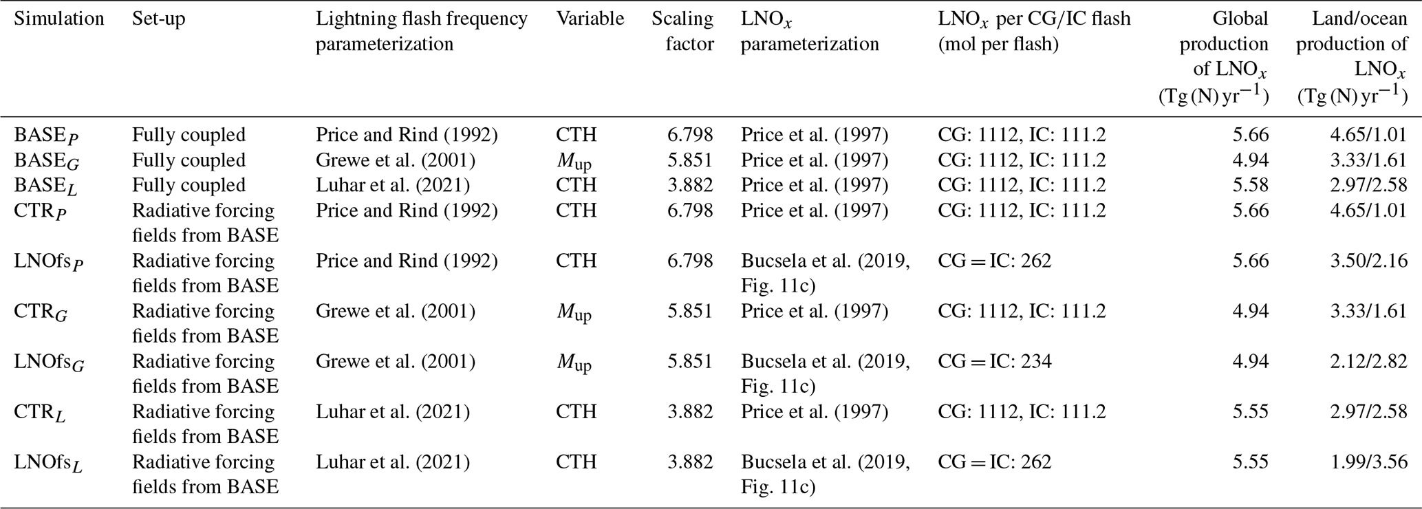
Price and Rind (1992)Price et al. (1997)Grewe et al. (2001)Price et al. (1997)Luhar et al. (2021)Price et al. (1997)Price and Rind (1992)Price et al. (1997)Price and Rind (1992)Bucsela et al. (2019, Fig. 11c)Grewe et al. (2001)Price et al. (1997)Grewe et al. (2001)Bucsela et al. (2019, Fig. 11c)Luhar et al. (2021)Price et al. (1997)Luhar et al. (2021)Bucsela et al. (2019, Fig. 11c)

Table 1 Overview of the performed simulations from 1 January 2000 to 1 January 2008. The subscript indicates the lightning parameterization: P represents Price and Rind (1992), G represents Grewe et al. (2001), and L represents Luhar et al. (2021). The variables that serve as a proxy for the lightning flash frequency are the cloud top height (CTH) and the upward flux of mass (M_up). The scaling factors to get ∼ 48 flashes per second during 2000 are included.

2.2 Climate–chemistry model and simulation set-ups

We employ the ECMWF–Hamburg (ECHAM)/Modular Earth Submodel System (MESSy version 2.55) Atmospheric Chemistry (EMAC) model (Jöckel et al., 2016) to perform three pairs of 8-year simulations using three different flash frequency parameterizations, with two different LNO_x schemes each. The simulations are conducted at a T42L90MA resolution, utilizing a quadratic Gaussian grid with box dimensions of approximately 2.8° × 2.8° in latitude and longitude. The model set-up covers 90 vertical levels that extend up to the 0.01 hPa pressure level, and a time step length of 720 s is employed (Jöckel et al., 2016). The lightning frequency is calculated at every time step and box by using the lightning parameterizations proposed by Price and Rind (1992), Grewe et al. (2001), or Luhar et al. (2021), being the latest modifications of the parameterization based on the CTH by Price and Rind (1992). In turn, we use scaling factors that ensure a global lightning occurrence rate of ∼ 48 flashes per second (Christian et al., 2003; Cecil et al., 2014). We refer to Pérez-Invernón et al. (2022b) for a detailed description of the performance of the parameterizations used in EMAC. In turn, we show the simulated annual spatial distributions of lightning flash density in Fig. S1 in the Supplement. LNO_x is calculated by using a modified version of the LNOX submodel of MESSy (Tost et al., 2007). Originally, the LNOX submodel imposes a constant amount of NO_x molecules emitted per flash that can be different or equal for CG and IC lightning based on Price et al. (1997). As a second step, the LNO_x molecules are vertically distributed by following a prescribed vertical profile that can vary latitudinally or between land and ocean, following the C-shaped vertical profiles reported by Pickering et al. (1998). We modify the LNOX submodel to include the LNO_x parameterization reported by Bucsela et al. (2019, Fig. 11c) and derived in Eq. (1).

We conduct the simulations using the quasi chemistry–transport model (QCTM) approach (Deckert et al., 2011). The QCTM mode allows for the separation of dynamics and chemistry in order to operate the model as a chemistry–transport model. This means that minor chemical changes do not introduce noise by affecting the simulated meteorology. The overview of the performed simulations are listed in Table 1, including the meteorological variables that serve as a proxy for lightning flash frequency, the scaling factors to get ∼ 48 flashes per second during 2000, and the production of LNO_x per flash and per year.

First, we perform three fully coupled free-running 8-year simulations (denoted BASE, where the subindex indicates the lightning flash frequency parameterization) from 1 January 2000 to 1 January 2008 to derive the forcings for the subsequent simulations. There is no consensus about the similarity or difference in the production of NO_x per flash depending on the type of lightning (Schumann and Huntrieser, 2007; Gordillo-Vázquez et al., 2019). However, climate–chemistry simulations usually set different LNO_x PE values for CG and IC lightning (Tost et al., 2007; Jöckel et al., 2016; Gordillo-Vázquez et al., 2019). In BASE simulations, we impose a production of 1112 mol per CG flash and 111.2 mol per IC flash, obtaining annual global emissions for LNO_x of 5.66, 4.94, and 5.58 Tg (N) yr⁻¹ for the lightning parameterizations by Price and Rind (1992) (subscript P), Grewe et al. (2001) (subscript G), and Luhar et al. (2021) (subscript L), respectively. These produced amounts per flash are based on the estimation of 6.7 × 10⁹ J per CG flash, 0.67 × 10⁹ J per IC flash, and 10 × 10¹⁶ $\mathrm{molec}.\left(\mathrm{NO}\right){\mathrm{J}}^{-\mathrm{1}}$ reported by Price et al. (1997). We employ the same chemical set-up and chemical mechanism as detailed by Jöckel et al. (2016) for the RC1-base-07 simulations.

The second set of simulations, here referred to as control (or CTR) simulations, are similar to the BASE simulations in terms of lightning and LNO_x parameterizations but using the radiative forcing fields from the BASE simulations, following the QCTM approach.

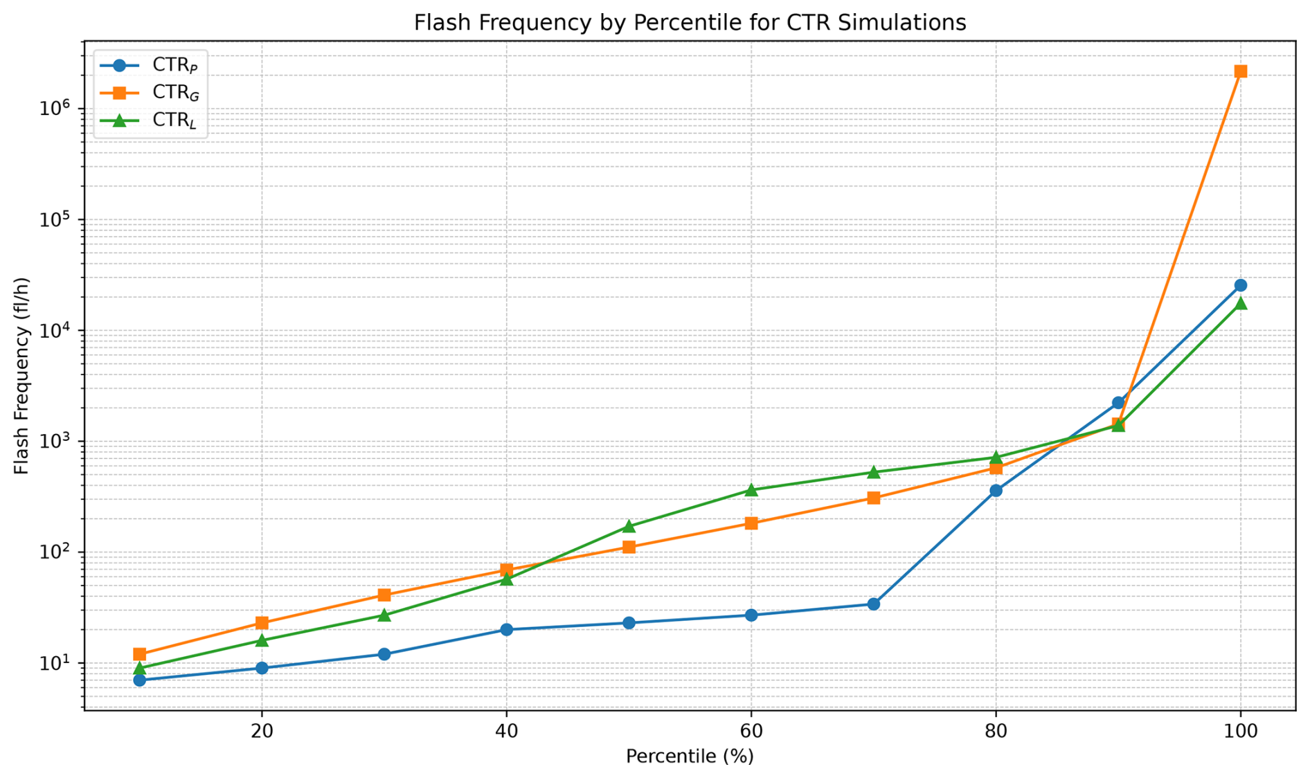
Figure 1 Fraction of 2.8° × 2.8° in latitude and longitude boxes (in percentile) containing less than a given instantaneous flash frequency in flashes per hour (“fl/h”) from the CTR simulations.

At this point, we explore the applicability of Eq. (1) within our model. Equation (1) is derived from data aggregated over 1° × 1° latitude–longitude grid boxes, whereas the simulations will be conducted using a coarser resolution of 2.8° × 2.8° grid boxes. We check that the percentage of boxes that contain a flash frequency lower than a specified value in the simulation and in the gridded data of Bucsela et al. (2019, Fig. 11c) are comparable. The data in Fig. 1 show the total number of flashes per hour in the 2.8° × 2.8° latitude and longitude boxes from EMAC. These values were estimated by selecting all the boxes at every output time step of 720 s (13 566 603 total samples) from the CTR simulations for the year 2000. These data allow us to ensure that the use of the LNO_x by Bucsela et al. (2019, Fig. 11c) is applicable in the LNOX submodel of MESSy. According to Bucsela et al. (2019), who used the World Wide Lightning Location Network (WWLLN) midlatitude lightning measurements corrected by the network's detection efficiency, nearly 90 % of the 1° × 1° boxes in latitude and longitude have flash rates lower than 2 kfl h⁻¹ (where kfl represents 1000 flashes), while we find that 90 % of the 2.8° × 2.8° boxes in latitude and longitude have flash rates lower than 2225, 1432, and 1386 kfl h⁻¹ (Fig. 1). In addition, comparison between the results of Bucsela et al. (2019, Fig. 11a) and Fig. 1 shows that the histogram of flashes per hour are roughly in agreement. This comparison of the instantaneous lightning frequency ensures the applicability of the LNO_x parameterization by Bucsela et al. (2019, Fig. 11c) in the LNOX submodel.

The third set of simulations, here referred to as “LNOfs” simulations, is similar to the set of CTR simulations but using the LNO_x parameterization reported by Bucsela et al. (2019, Fig. 11c) and scaling the total emissions of NO_x from Eq. (1) to obtain the same total emissions of LNO_x as in the CTR simulations.

We use three lightning flash frequency parameterizations and the same LNO_x vertical profile (Pickering et al., 1998) in all the simulations to isolate the effect of the LNO_x production parameterization on the chemical composition of the atmosphere. However, other lightning parameterizations (Tost et al., 2007) and vertical profiles of LNO_x (Ott et al., 2010) can also be used, possibly producing slight variations in the results.

3 Results and discussion

3.1 Total emissions of LNO_x

We extract the global total (CG + IC) flash frequency and the total amount of LNO_x at every output time step of 720 s during 2000 to estimate the global distribution of the produced LNO_x per year from the CTR and LNOfs simulations. Figure 2 shows the mean daily data for June–July–August (JJA) of LNO_x obtained from the CTR and LNOfs simulations, as well as the difference between them. We select the season JJA to facilitate the comparison with OMI-WWLLN-based measurements by Bucsela et al. (2019, Fig. 3). The LNOfs simulations predict a larger amount of LNO_x over the tropical ocean, where thunderstorms have a lower lightning frequency than over land. In turn, the decrease in the production of LNO_x is larger over land in tropical regions than in midlatitudes, as tropical thunderstorms are more active. The LNOfs_P and LNOfs_G simulations present a smoother distribution of the LNO_x distribution over land than the CTR_P and the CTR_G simulations, with a significant decrease in the peak production of LNO_x in North America. The difference of the land/ocean contrast of the production of LNO_x between the CTR_L and LNOfs_L simulations is lower, because the parameterization by Luhar et al. (2021) detects more active thunderstorms over the oceans. In terms of the spatial distribution of LNO_x production, the parameterizations based on lightning flash frequency rates reduces differences between the three employed lightning parameterizations. The differences between the LNOfs and CTR simulations can also be seen in the difference between the annual-averaged mixing ratios of NO_x at the 800 hPa pressure level (Fig. 3). The new parameterization of the production of LNO_x produces larger emissions of LNO_x over oceans, except for the high-latitude oceanic regions in the LNOfs_G simulation, where we obtain a smaller production of LNO_x than in the CTR_G simulation. The reason of this difference is that the lightning parameterization by Grewe et al. (2001) detects more active and sparse thunderstorms in these oceanic regions than the parameterizations based on the CTH (Tost et al., 2007, Fig. 2). The spatial distribution of the mean monthly LNO_x obtained from the LNOfs simulations during 2000 is shown in Fig. S2. During 1 complete year, the parameterizations based on the CTH (LNOfs_P and LNOfs_L simulations) produce a smoother spatial distribution of LNO_x, while the parameterization by Luhar et al. (2021) (LNOfs_L simulation) produced relatively more LNO_x over the oceans.

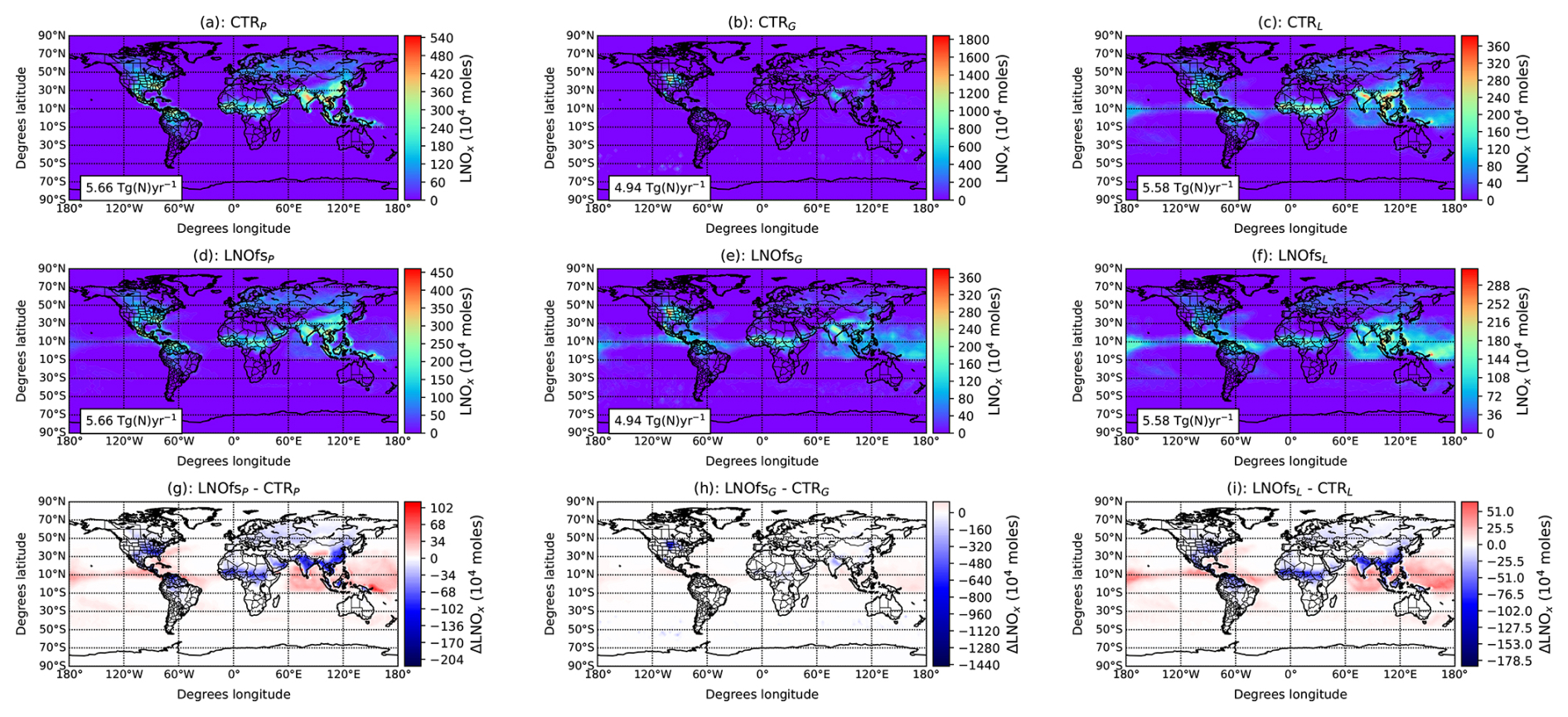
Figure 2 Daily mean LNO_x production (× 10⁴ moles) in June–July–August (JJA) per 2.8° latitude × 2.8° longitude box obtained from the CTR (a–c) and the LNOfs (d–f) simulations. Panels (g–i) show the difference between CTR and LNOfs simulations. Note that the colour scales are different in each panel.

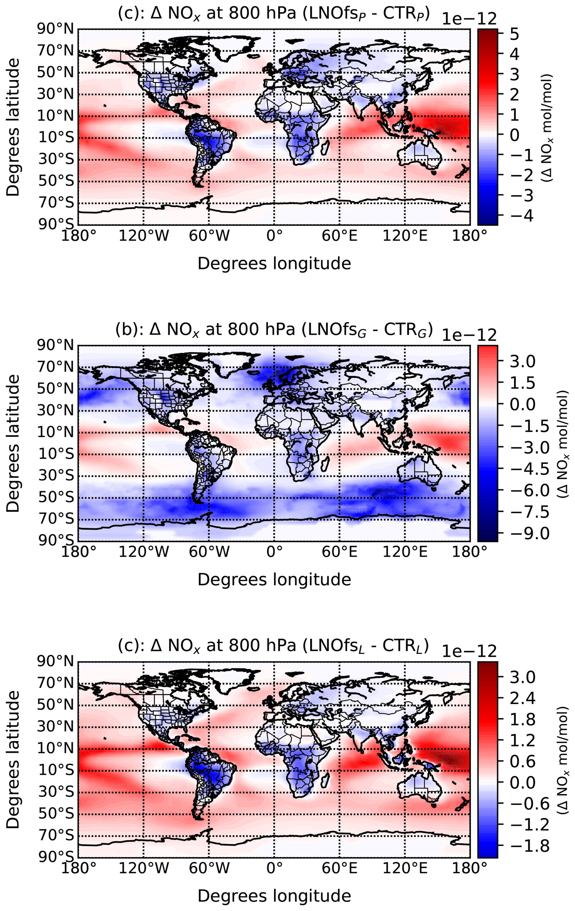
Figure 3 Annually (2002–2007) and globally averaged differences in the mixing ratio of NO_x between the simulations with the LNO_x production based on the flash frequency (LNOfs) and the simulation with a constant quantity of LNO_x production per flash (CTR) at the 800 hPa pressure level. The subscript indicates the lightning parameterization: P represents Price and Rind (1992), G represents Grewe et al. (2001), and L represents Luhar et al. (2021).

When comparing Fig. 2 to the mean daily LNO_x emissions during JJA as reported by Bucsela et al. (2019, Fig. 3c), it becomes apparent that the LNO_x parameterization based on the lightning frequency in the LNOfs simulations produces a spatial distribution of LNO_x that aligns with space-based measurements more accurately (Bucsela et al., 2019, Fig. 3c) than the parameterization used in the CTR simulations. In particular, LNO_x emissions over the ocean in the CTR_P and CTR_G simulations are too low to be noticeable compared to those over land, whereas they are larger in Bucsela et al. (2019, Fig. 3c). However, the LNOf_P and LNOfs_G simulations produce significant LNO_x emissions over the oceans. Apart from that, the LNOfs simulations yield a spatial distribution of LNO_x that exhibits a more homogeneous distribution in the tropics and midlatitudes compared to the CTR simulations.

3.2 Implications for the chemical composition of the troposphere

We compare the effect of LNO_x on the chemistry of the troposphere between the CTR and LNOfs simulations. The spatial distributions of the annual global difference in the mixing ratio of the analysed chemical species at the 600, 400, and 200 hPa pressure levels between the LNOfs and CTR simulations are shown in the Supplement (Figs. S3–S11 in the Supplement). Figures 4 and 5 show the implications of using an LNO_x parameterization based on the flash frequency in the annually and zonally averaged vertical profiles of NO_x = NO + NO₂, O₃, CO, HO_x = OH + HO₂, HNO₃, and HNO₄. The vertical profile of N₂O is not shown because the variations are negligible, as expected (absolute value lower than −0.005 %). We exclude plots of LNOf_L from Figs. 4 and 5, because the influence of the new parameterization of LNO_x production is spatially similar to that in the LNOf_P simulations but reduced in absolute value (see Figs. S3–S11). The first column of Figs. 4 and 5 shows the annually and zonally averaged vertical profiles of the mixing ratios of these species from the CTR_P simulation, the second column shows the differences in the profiles between the LNOfs_P and the CTR_P simulations, and the third column shows the differences in the profiles between the LNOfs_G and the CTR_G simulations.

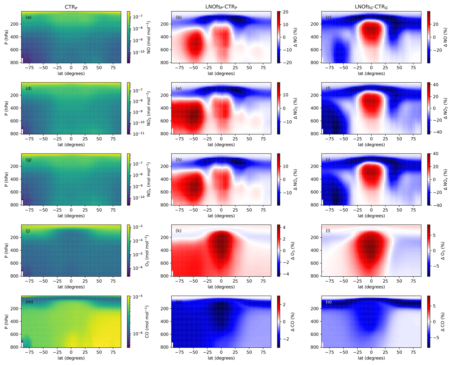
Figure 4 First column: annually (2002–2007) and zonally averaged vertical profiles of the NO, NO₂, NO_x, O₃, and CO mixing ratios for a simulation with a constant amount of LNO_x production per flash (CTR_P). Second column: differences (in %) between the annually and globally averaged mixing ratio of the chemical species from the simulation with the LNO_x production based on the flash frequency (LNOfs_P) and from the CTR_P simulation. Third column: same as the first column but showing differences between the LNOfs_G and CTR_G simulations. The differences have been calculated as $\mathrm{100}\times (\mathrm{LNOfs}-\mathrm{CTR})/\mathrm{CTR}$. The subscript indicates the lightning parameterization: P represents Price and Rind (1992) and G represents Grewe et al. (2001).

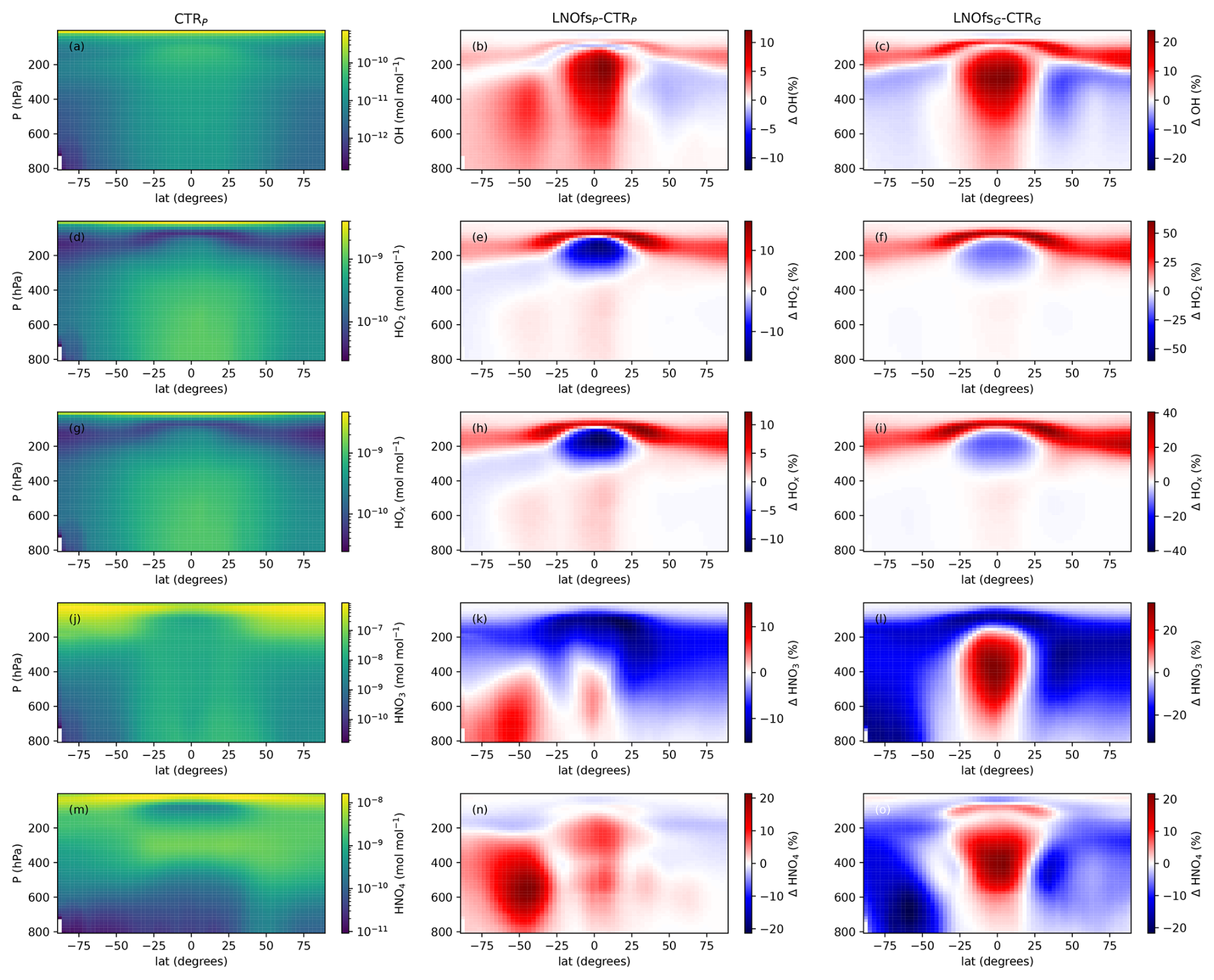
Figure 5 First column: annually (2002–2007) and zonally averaged vertical profiles of the OH, HO₂, HO_x, HNO₃, and HNO₄ mixing ratios for a simulation with a constant amount of LNO_x production per flash (CTR_P). Second column: differences (in %) between the annually and globally averaged mixing ratio of the chemical species from the simulation with the LNO_x production based on the flash frequency (LNOfs_P) and from the CTR_P simulation. Third column: same as the first column but showing differences between the LNOfs_G and CTR_G simulations. The differences have been calculated as $\mathrm{100}\times (\mathrm{LNOfs}-\mathrm{CTR})/\mathrm{CTR}$. The subscript indicates the lightning parameterization: P represents Price and Rind (1992) and G represents Grewe et al. (2001).

The LNOfs simulations produce a larger mixing ratio of NO, NO₂, and NO_x in the middle level of the tropical troposphere (around 350 hPa in Fig. 4a–i) than the corresponding CTR simulations. However, the mixing ratio of NO_x at altitudes above the 300 hPa pressure level is larger in the CTR simulations. In addition, Fig. 3 indicates that the difference at the 800 hPa pressure level is larger (more positive) over the ocean, where the flash frequency for thunderstorms is lower. In turn, the differences are lower (more negative) in the lightning chimneys over land in Africa, North America, and South America, where the flash frequency is notably higher. At the 200 hPa level (Figs. S9–S11a), the differences in NO_x mixing ratio between the LNOfs and CTR simulations are negative in more areas. The spatial distributions of the NO_x mixing ratios in Figs. S9–S11a indicate that the mixing ratio of NO_x in the upper troposphere is lower in the LNOfs simulations, because more LNO_x is emitted in weak thunderstorms (thunderstorms with a lower flash frequency) that are less efficient in elevating the LNO_x to the upper troposphere. Therefore, the parameterization of LNO_x production based on the flash frequency (LNOfs simulations) leads to a lower contribution of lightning to the sources of NO_x of the upper troposphere compared to the CTR simulations. There are differences in the vertical profile of the variation of NO_x between the LNOfs_P and LNOfs_G simulations, as can be seen by comparing Fig. 4h and Fig. 4i. Below the 500 hPa pressure level, the difference of the mixing ratio of NO_x between the LNOfs_P and CTR_P simulations is positive, while the opposite is found when comparing the LNOfs_G with the CTR_G simulations. Nevertheless, these differences are small, both in absolute and in relative terms. We consider that these small differences are due to the fact that in the CTR simulations the LNO_x depends on the $\mathrm{CG}/\mathrm{IC}$ ratio, while in LNOfs simulations both CG and IC produce the same amount of LNO_x.

Differences in the NO_x mixing ratio between the LNOfs and CTR simulations cause differences in other chemical species. The obtained differences in the mixing ratios of O₃ between the LNOfs and CTR simulations are connected to the different spatial distributions of LNO_x production. LNO_x can produce or deplete O₃ depending on the background mixing ratio of NO_x caused by photochemistry (Crutzen, 1979; Schumann and Huntrieser, 2007; Liu, 1977; Verma et al., 2021). The NO directly produced by lightning can destroy O₃ by chemical reaction (Levine et al., 1984)

$$\begin{array}{}\text{(2)}& \mathrm{NO}+{\mathrm{O}}_{\mathrm{3}}\to {\mathrm{NO}}_{\mathrm{2}}+{\mathrm{O}}_{\mathrm{2}},\end{array}$$

and the resulting NO₂ can produce atomic oxygen by photolysis following the reaction (Levine et al., 1984):

$$\begin{array}{}\text{(3)}& {\mathrm{NO}}_{\mathrm{2}}+h\mathit{\nu }\to \mathrm{NO}+\mathrm{O}.\end{array}$$

Finally, the produced atomic oxygen can increase the mixing ratio of O₃ by interacting with a third body M (Levine et al., 1984) as

$$\begin{array}{}\text{(4)}& \mathrm{O}+{\mathrm{O}}_{\mathrm{2}}+M\to {\mathrm{O}}_{\mathrm{3}}+M.\end{array}$$

Overall, LNO_x contributes to ozone depletion in regions with low background mixing ratio of NO_x, such as over the tropical marine boundary layer. In turn, LNO_x produces ozone in regions where the background mixing ratio of NO_x is high, such as over the continents. Figure 4j–l illustrate that the LNOfs simulations lead to a larger mixing ratio of ozone in the lower and middle troposphere caused by a larger production of LNO_x at these vertical levels, especially in the tropics. Additionally, the larger production of LNO_x results in very low changes in the ozone mixing ratio in the upper troposphere, due to the presence of a high NO_x background. At these higher altitudes, the efficiency of ozone production by NO_x is larger, but the emitted LNO_x is lower. Figures S6–S8b indicate that the larger positive change in the mixing ratio of O₃ at the 400 hPa level is located at oceanic regions, where the LNOfs simulation produces more LNO_x than the CTR simulation. In turn, the LNOfs simulations produce a lower mixing ratio of O₃ in the tropical Atlantic Ocean, where the background O₃ is not produced by local oceanic thunderstorms but by LNO_x transported from land. Figures 6–9 show the seasonal total column-integrated O₃ between the ground and the top of the troposphere. During December–January–February (DJF), winter thunderstorms in the Northern Hemisphere are less intense than in other seasons. On the contrary, summer thunderstorms in South America and Australia are more active. This is visible in Fig. 6, showing that the tropospheric column of ozone is larger over the continents in the Northern Hemisphere in the LNOfs simulations and smaller or similar over land in South America, Australia, and southern Africa. During JJA (Fig. 8), the opposite situation occurs. Winter thunderstorms over the continents of the Southern Hemisphere lead to an increase in tropospheric ozone in the LNOfs simulations, while continental summer thunderstorms in the Northern Hemisphere produce less ozone. During the MAM and SON seasons (Figs. 7 and 9), lightning activity is more homogeneously distributed across the globe, resulting in the major changes in the tropospheric ozone column in the LNOfs simulations being primarily confined to land/ocean contrasts. More ozone is produced over the oceans, where less-active thunderstorms produce more LNO_x than in the CTR simulations. The main difference between the LNOfs_P and the LNOfs_G simulations can be seen during the DJF season. During DJF, more tropospheric ozone is produced in the LNOfs_P simulations compared to CTR_P, while less tropospheric ozone is produced in the LNOfs_G simulations than in CTR_G.

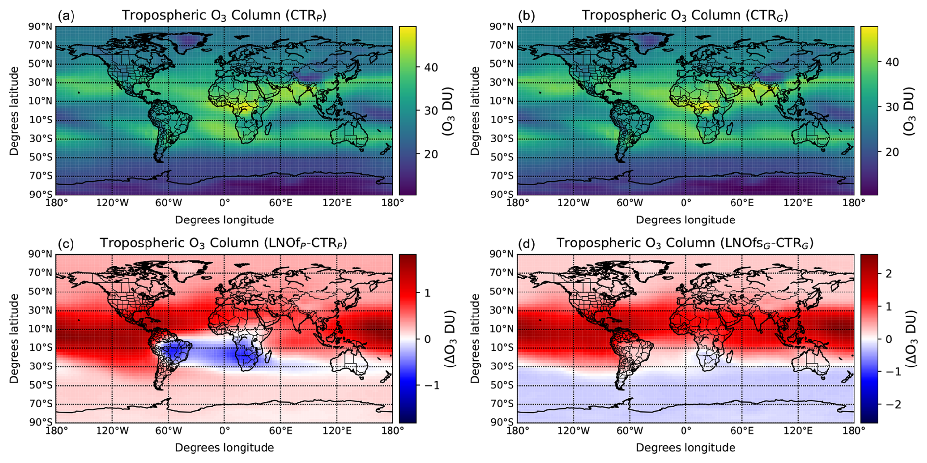
Figure 6 Global tropospheric column of O₃ in the CTR simulations (a, b) and differences in the O₃ total column (integrated between the ground and the top of the troposphere) between the LNOfs and CTR simulations (c, d) averaged during DJF (2002–2007). The values are given in Dobson Units (DU). The subscript indicates the lightning parameterization: P represents Price and Rind (1992) and G represents Grewe et al. (2001). The monthly total O₃ column from the CTR_L simulation can be seen in Figs. S3–S14.

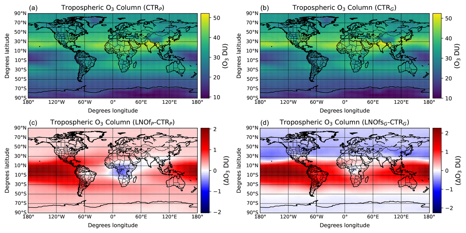
Figure 7 Global tropospheric column of O₃ in the CTR simulations (a, b) and differences in the O₃ total column (integrated between the ground and the top of the troposphere) between the LNOfs and CTR simulations (c, d) averaged during MAM (2002–2007). The values are given in Dobson Units (DU). The subscript indicates the lightning parameterization: P represents Price and Rind (1992) and G represents Grewe et al. (2001). The monthly total O₃ column from the CTR_L simulation can be seen in Figs. S3–S14.

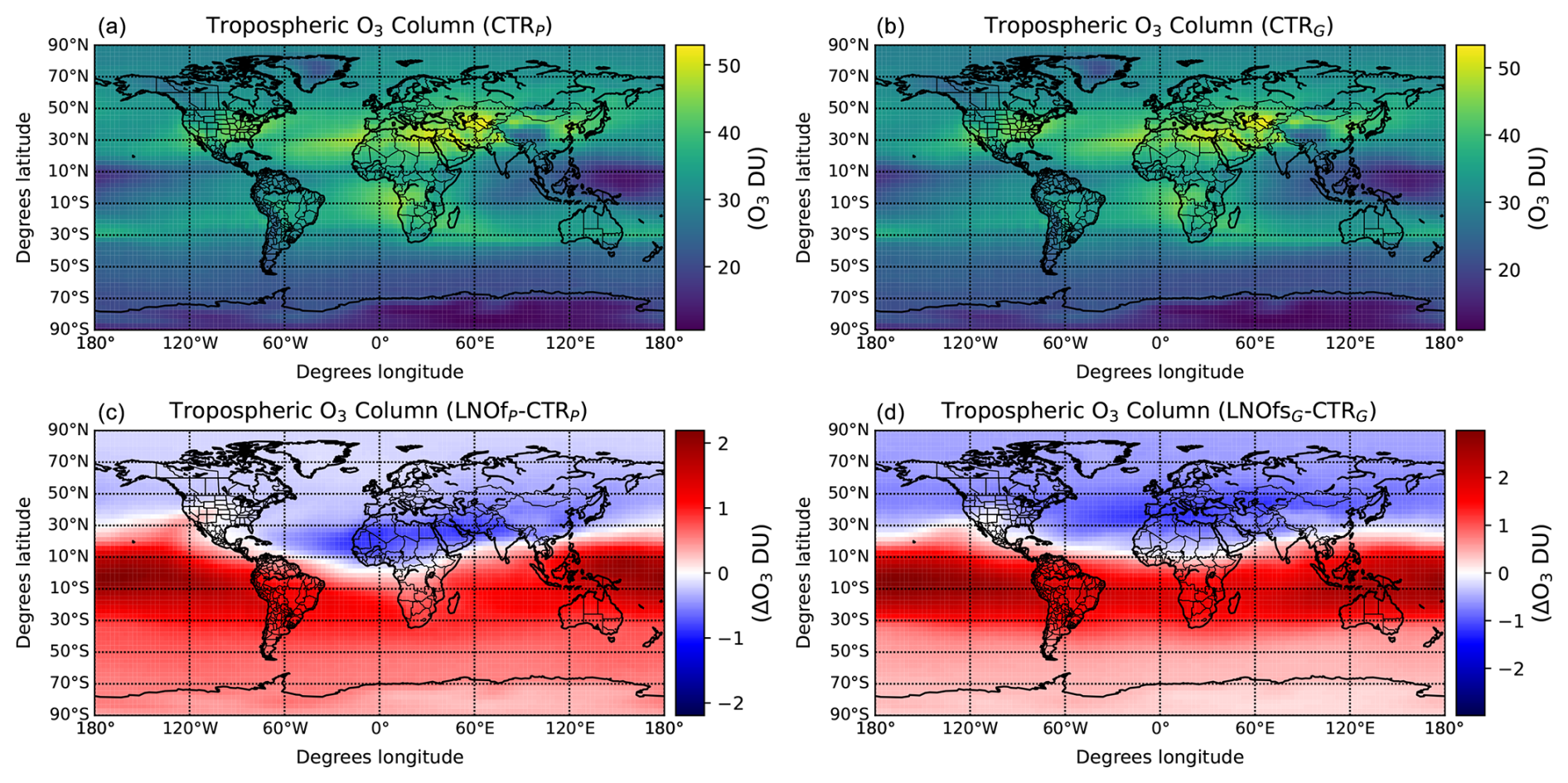
Figure 8 Global tropospheric column of O₃ in the CTR simulations (a, b) and differences in the O₃ total column (integrated between the ground and the top of the troposphere) between the LNOfs and CTR simulations (c, d) averaged during JJA (2002–2007). The values are given in Dobson Units (DU). The subscript indicates the lightning parameterization: P represents Price and Rind (1992) and G represents Grewe et al. (2001). The monthly total O₃ column from the CTR_L simulation can be seen in Figs. S3–S14.

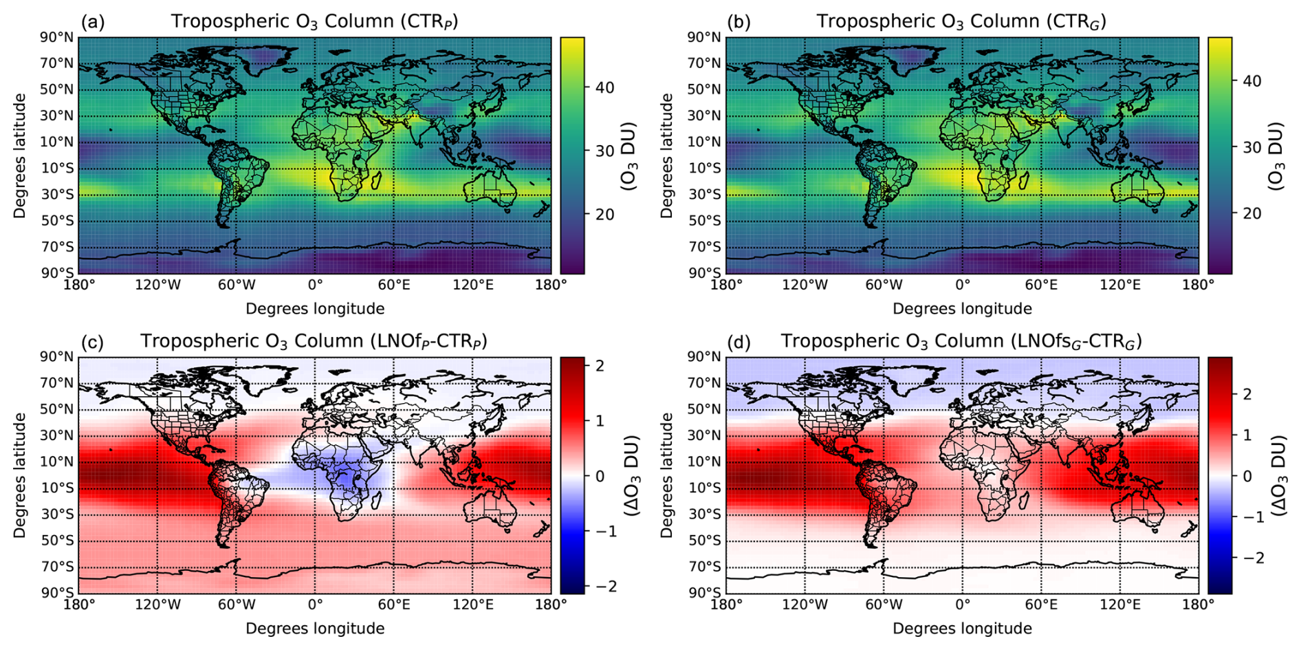
Figure 9 Global tropospheric column of O₃ in the CTR simulations (a, b) and differences in the O₃ total column (integrated between the ground and the top of the troposphere) between the LNOfs and CTR simulations (c, d) averaged during SON (2002–2007). The values are given in Dobson Units (DU). The subscript indicates the lightning parameterization: P represents Price and Rind (1992) and G represents Grewe et al. (2001). The monthly total O₃ column from the CTR_L simulation can be seen in Figs. S3–S14.

The relationship between HO_x and LNO_x is not linear (Schumann and Huntrieser, 2007). Under clean-air conditions and in medium-polluted regions, OH is produced as a consequence of LNO_x by O₃ and NO₂ photolysis. However, in regions with large amounts of NO_x, LNO_x contributes to a depletion of the HO₂ mixing ratio by reactions between NO₂ and HO₂, contributing to a decrease in the HO_x mixing ratio. At the 600 hPa level (Figs. S3–S5), where in general the background NO_x is low, increases of NO_x lead to increases of HO_x (Figs 5d–i and S3–S5). We obtain the opposite situation at the 200 hPa level, where the background NO_x is large (Figs 5d-i and S9–S11). At the 400 hPa pressure level, where the background NO_x is medium in comparison with other vertical levels (Fig. 4)g, the relationship between NO_x and HO_x is more complex (Figs. 5d-i and S6–S8).

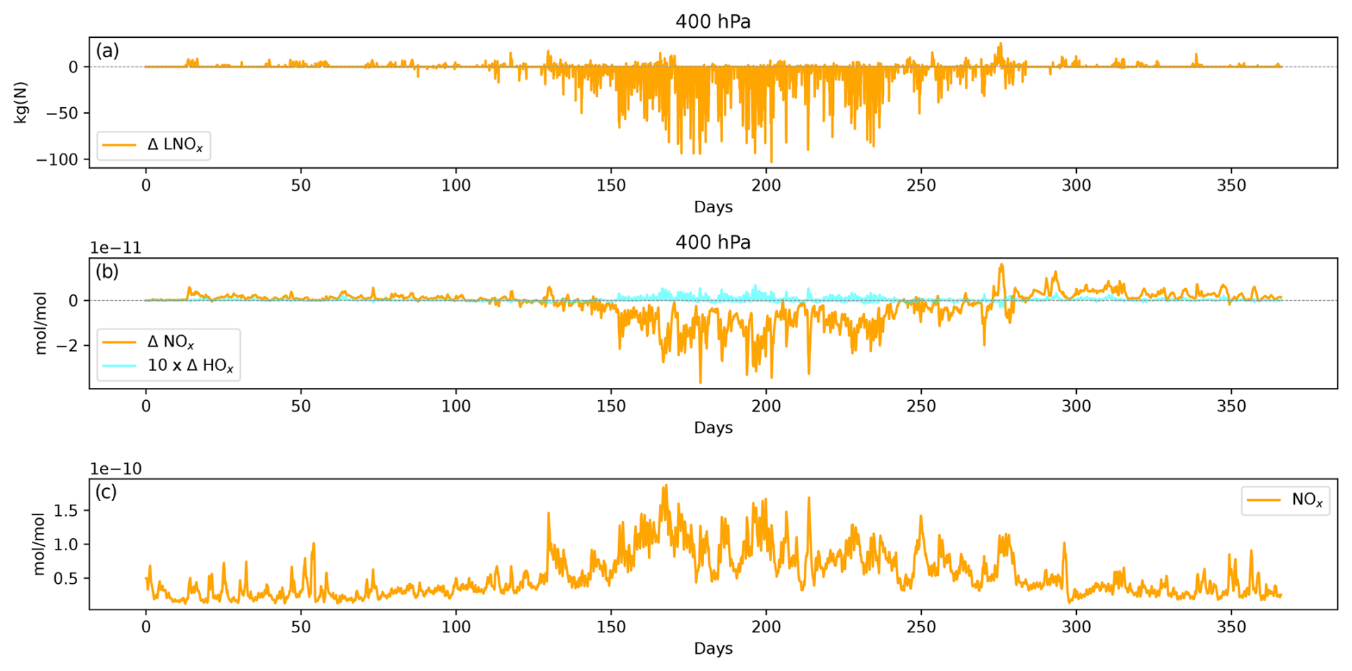
Figure 10 (a) Difference in the hourly total column production of LNO_x between the LNOfs_L and CTR_L simulations over a 1-year period (day 1 corresponds to 1 January 2000). (b) Hourly differences in the mixing ratios of NO_x and HO_x at the 400 hPa. (c) Hourly background mixing ratio of NO_x at the 400 hPa level in the LNOfs_L simulation. The three panels correspond to a spatial average over Europe (bounded by 42 to 52° N latitude and by 0 to 24° E longitude). The subscript P indicates the lightning parameterization: Price and Rind (1992).

To exemplify the influence of LNO_x on the mixing ratio of HO_x, we show the impact of LNO_x on the HO_x mixing ratio in the geographical region of Europe (bounded by 42 to 52° N latitude and by 0 to 24° E longitude) in Fig. 10. The first panel illustrates the disparity in the hourly total column emissions of LNO_x between the LNOfs_L and CTR_L simulations over a 1-year period, where negative values represent a reduced LNO_x production in the LNOfs_L simulation. In the second panel, the hourly differences in the NO_x and HO_x mixing ratios at the 400 hPa level are shown. Lastly, the third panel shows the hourly background mixing ratio of NO_x at the 400 hPa level. Before day 140, when the background mixing ratio of NO_x is low, changes in NO_x and HO_x follow the same trend. Conversely, during the summer when the background mixing ratio of NO_x is large, the changes in NO_x and HO_x are of opposite signs, implying that increased NO_x leads to a decrease in the mixing ratio of HO_x.

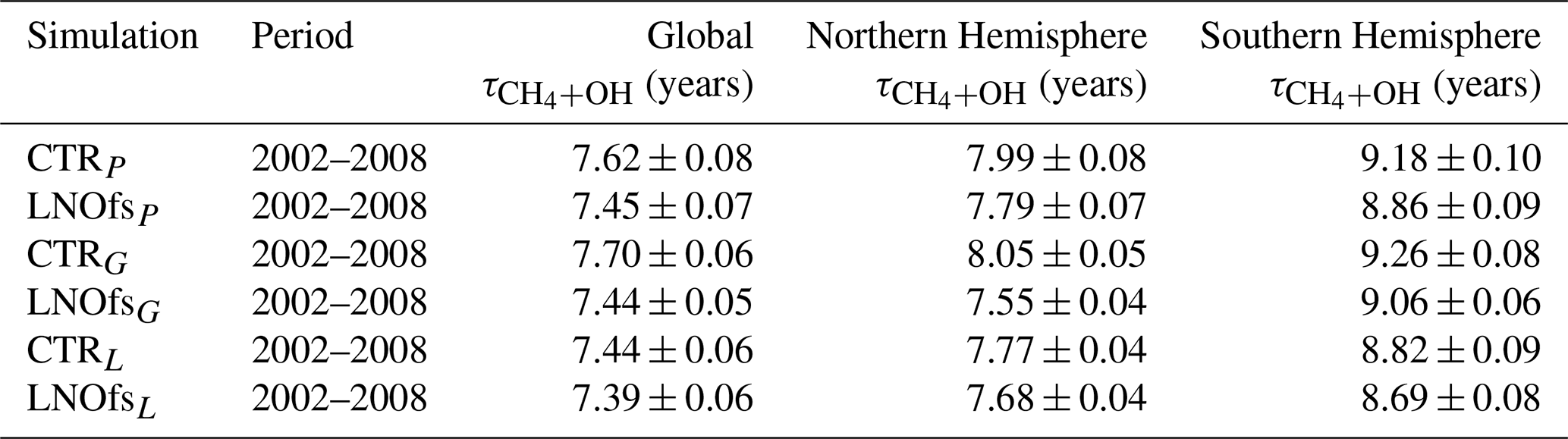
Table 2 Annually averaged tropospheric methane lifetime with respect to OH (${\mathit{\tau }}_{{\mathrm{CH}}_{\mathrm{4}}+\mathrm{OH}}$) in years and standard deviation resulting from different simulation results.

In Figs. S12 and S13, we show analogous plots to Fig. 10 but at different pressure levels (200 and 600 hPa, respectively). At the 200 hPa level, characterized by a large background mixing ratio of NO_x (see Fig. 4g), the changes in NO_x and HO_x exhibit opposing behaviours. Conversely, at the 600 hPa level, where the background mixing ratio of NO_x is low (see Fig. 4g), the changes in NO_x and HO_x follow the same trend. In turn, we gather the background mixing ratio of NO_x across each cell domain at 200, 400, and 600 hPa pressure levels during hours when the changes in NO_x and HO_x share the same sign, resulting in an average mixing ratio of NO_x at 7.2 × 10⁻¹¹ mol mol⁻¹. Conversely, when the changes in NO_x and HO_x are of opposite signs, the averaged mixing ratio of NO_x is 1.8 × 10⁻¹⁰ mol mol⁻¹. The observed disparity of the NO_x background mixing ratio under conditions of opposite sign changes confirms that the influence of LNO_x on the mixing ratio of HO_x is largely dependent on the background mixing ratio of NO_x. Additional details regarding the distribution of the background mixing ratio of NO_x under similar or opposite sign variations are shown in the Supplement.

Figures 4m–o and 5a–c show a clear inverse correlation between the variation of OH and CO, given that the CO in the troposphere is removed by OH through

$$\begin{array}{}\text{(5)}& \mathrm{CO}+\mathrm{OH}\to {\mathrm{CO}}_{\mathrm{2}}+\mathrm{H}.\end{array}$$

The differences between the mixing ratios of HNO₃ and HNO₄ between the simulations can all be explained by the differences in NO_x. In the troposphere, LNO_x contributes to the production of HNO₃ and HNO₄. Therefore, in the LNOfs simulations, smaller mixing ratios of NO_x in the upper troposphere lead to lower mixing ratios of these species (Fig. 5j–o). The global annual means shown in Figs. S3–S11e and f indicate that the reduction of HNO₃ and HNO₄ in the LNOfs simulations is larger in the upper troposphere over land, while increased mixing ratios are located over ocean.

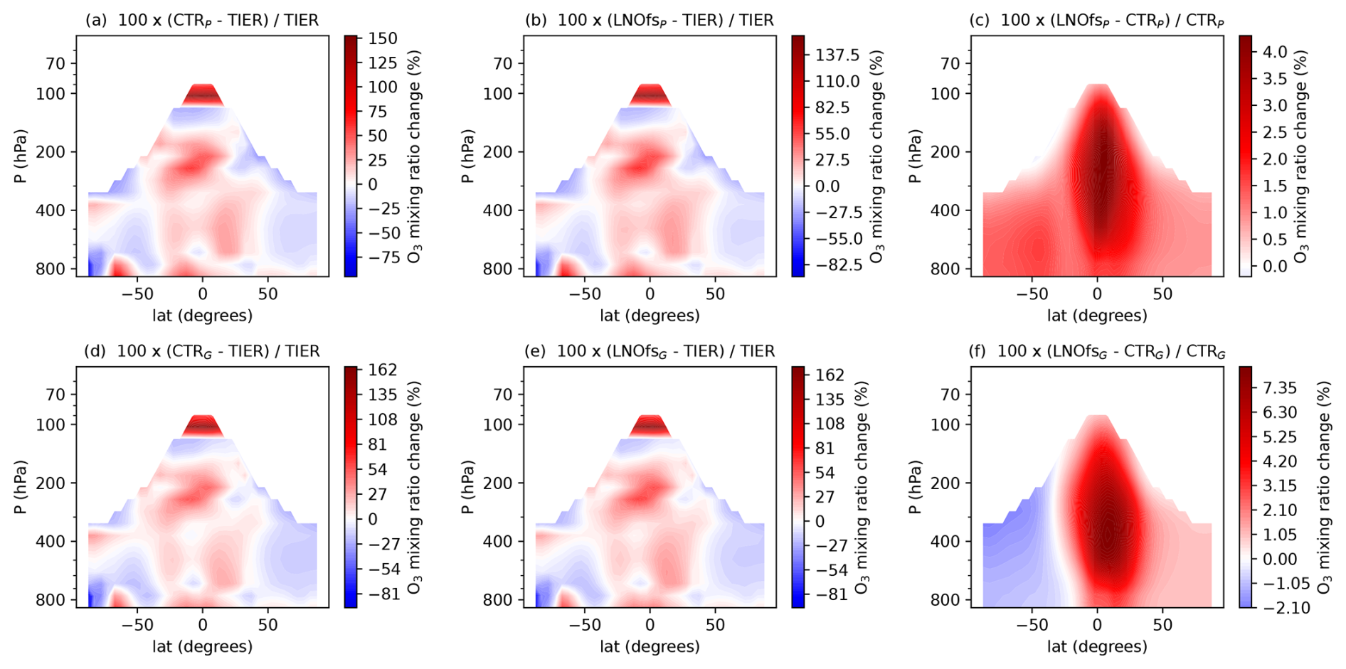
Figure 11 Seasonally (DJF) and zonally averaged differences (in %) in the vertical O₃ mixing ratio between the simulations and the Bodeker Scientific global vertically resolved ozone database Tier 1.4 vn1.0 product Hassler et al. (2009). The border with the white region represents the zonally averaged mean altitude of the climatological tropopause. The subscript indicates the lightning parameterization: P represents Price and Rind (1992) and G represents Grewe et al. (2001).

The OH radical is a significant oxidant that reacts with methane (CH₄), influencing its atmospheric lifetime. Therefore, variations in the mixing ratio of OH caused by different parameterizations of LNO_x production can potentially affect the lifetime of CH₄. We calculate the tropospheric lifetime of CH₄ with respect to OH (${\mathit{\tau }}_{{\mathrm{CH}}_{\mathrm{4}}+\mathrm{OH}}$) on a monthly basis using Jöckel et al. (2016, Eq. 1). Table 2 shows the annually averaged tropospheric methane lifetime with respect to OH resulting from different simulations, together with the standard deviation. To calculate the means shown in Table2, we first compute the mean for each simulated year based on the monthly means of the 12 months. Then, we calculate the overall mean and standard deviation as the average and the standard deviation of the yearly means. At a global scale, the annually averaged lifetime of methane with respect to OH in the LNOfs simulations is reduced by 2.2 %, 3.4 %, and 0.7 % for the lightning parameterizations P, G, and L, respectively. We use the mean and standard deviation to compute the p value of a two-sample t test to assess the significance of differences in methane lifetime. A p value threshold of 0.05 is used to determine statistical significance. The results indicate that the differences between CTR and LNOfs are significant in the P and G simulations, with p values of 3 × 10⁻³ and 10⁻⁵, respectively. In contrast, no significant differences are observed in the L simulations, as the obtained p value is 0.2. In the Northern Hemisphere, the corresponding decreases are 2.5 %, 6.2 %, and 1.2 %, respectively. In turn, we obtain decreases of 3.5 %, 2.2 %, and 1.5 % in the Southern Hemisphere. The decreases are larger in the Southern Hemisphere, where more LNO_x is emitted due to the larger oceanic area than in the Northern Hemisphere. The new parameterization of the LNO_x production affects the lifetime of methane in the P and the G simulations more than in the L simulations. The reduction of the global methane lifetime with respect to OH deviates from that obtained by the multimodel mean of 9.7 ± 1.5 years (Naik et al., 2013).

3.3 Comparison with data of zonal ozone distribution

The simulated zonal ozone distribution from the CTR and LNOfs simulations can be compared with ozone profile data from Hassler et al. (2009) and Bodeker (2014), as previously carried out by Luhar et al. (2021), to assess the impact of different lightning parameterizations on global ozone mixing ratios. The Bodeker Scientific global vertically resolved ozone database includes monthly mean vertical ozone profiles spanning from 1979 to 2016 across 70 vertical levels. In this study, we utilize the Tier 1.4 vn1.0 product, specifically the version containing the mean annual cycle derived from anthropogenic, natural, and volcanic emissions. We regrid the data to match the resolution of the model. The comparison between the simulated seasonal zonal ozone distribution and the Bodeker Scientific global vertically resolved ozone database Tier 1.4 vn1.0 product between 2002 and 2007 is shown in Figs. 11–14. During all the seasons, the LNOfs simulations produce more tropospheric ozone than the corresponding CTR simulations in the tropics, causing more disagreement with measurements than the CTR simulations. The effect of the LNOfs simulations in the midlatitude tropospheric ozone varies with the lightning parameterization and with the seasons. For DJF, the new parameterization of the production of LNO_x produces a larger content of tropospheric ozone in the Northern Hemisphere, contributing to a better agreement with measurements. In the Southern Hemisphere, the LNOfs simulations produce more tropospheric ozone in the P simulations but less ozone in the G simulations, producing a better agreement with the measurements only in the case of the P simulations. For MAM, the LNOfs_P simulation shows more ozone in both hemispheres, while the LNOfs_G simulations result in more ozone in the tropics but less ozone in the midlatitudes in both hemispheres. In this case, only the LNOfs_P simulations show a better agreement with the measurements and only in the Northern Hemisphere. For JJA, the LNOfs simulations result in a better agreement with observations in the Southern Hemisphere, and less agreement in the Northern Hemisphere. For SON, the LNOfs simulations show a better agreement with the measured tropospheric ozone in the Southern Hemisphere and a worse agreement in the Northern Hemisphere.

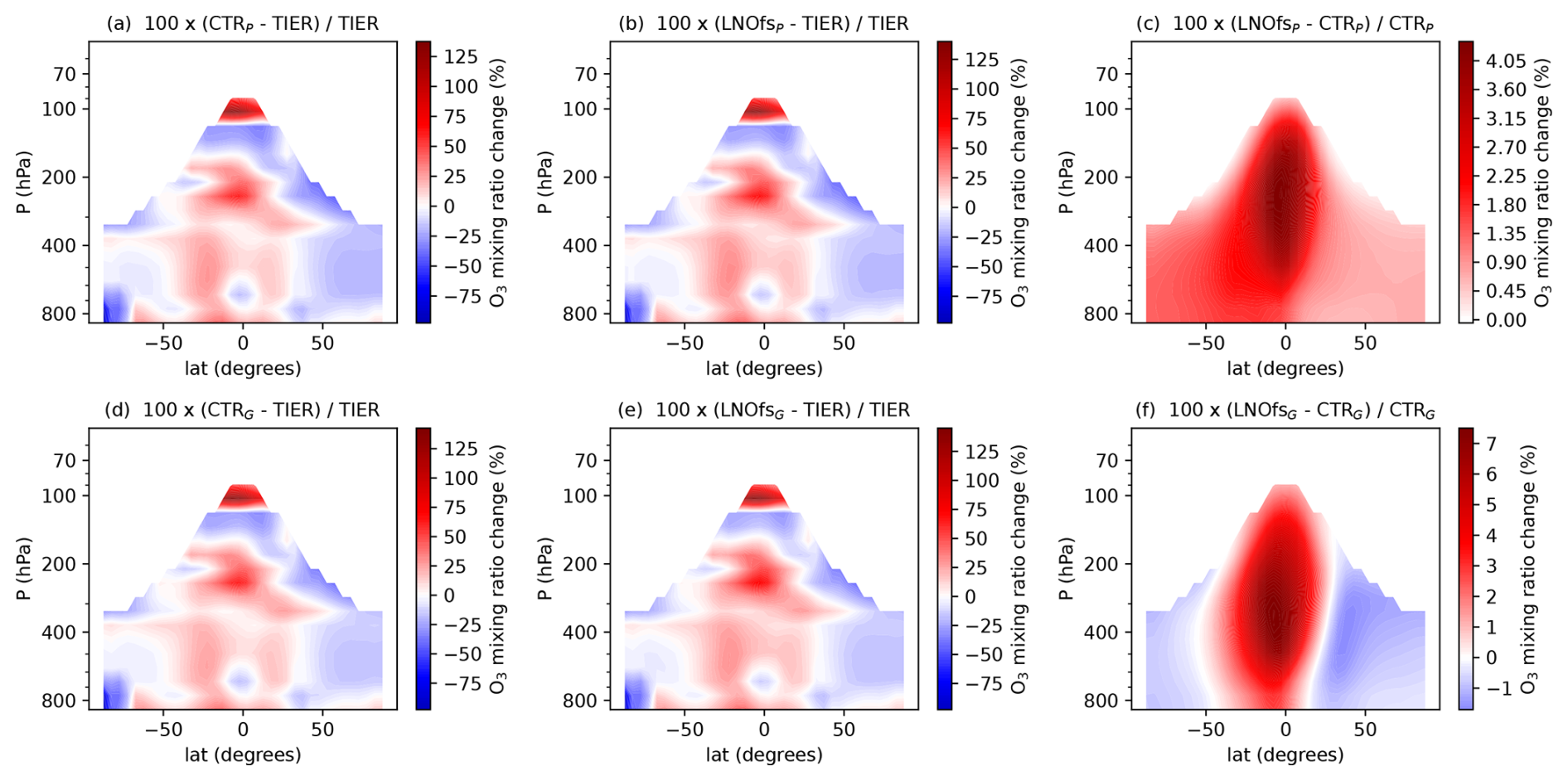
Figure 12 Seasonally (March–April–May, MAM) and zonally averaged differences (in %) in the vertical O₃ mixing ratio between the simulations and the Bodeker Scientific global vertically resolved ozone database Tier 1.4 vn1.0 product Hassler et al. (2009). The border with the white region represents the zonally averaged mean altitude of the climatological tropopause. The subscript indicates the lightning parameterization: P represents Price and Rind (1992) and G represents Grewe et al. (2001).

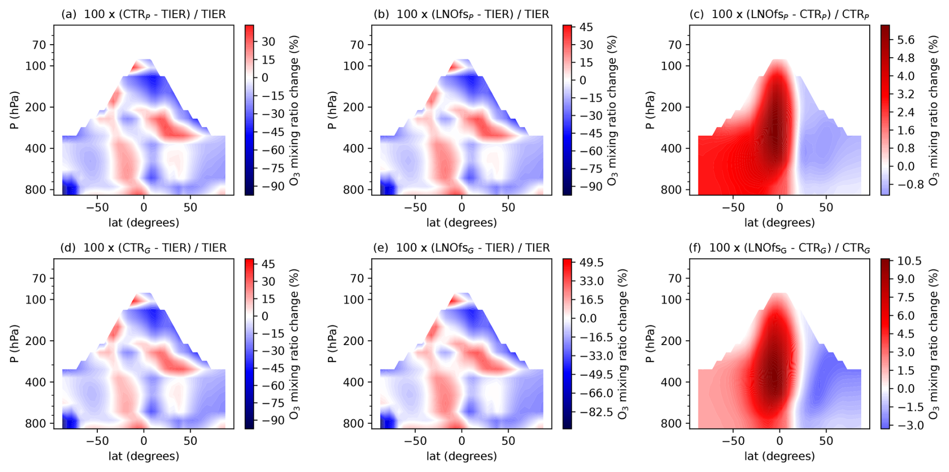
Figure 13 Seasonally (JJA) and zonally averaged differences (in %) in the vertical O₃ mixing ratio between the simulations and the Bodeker Scientific global vertically resolved ozone database Tier 1.4 vn1.0 product Hassler et al. (2009). The border with the white region represents the zonally averaged mean altitude of the climatological tropopause. The subscript indicates the lightning parameterization: P represents Price and Rind (1992) and G represents Grewe et al. (2001).

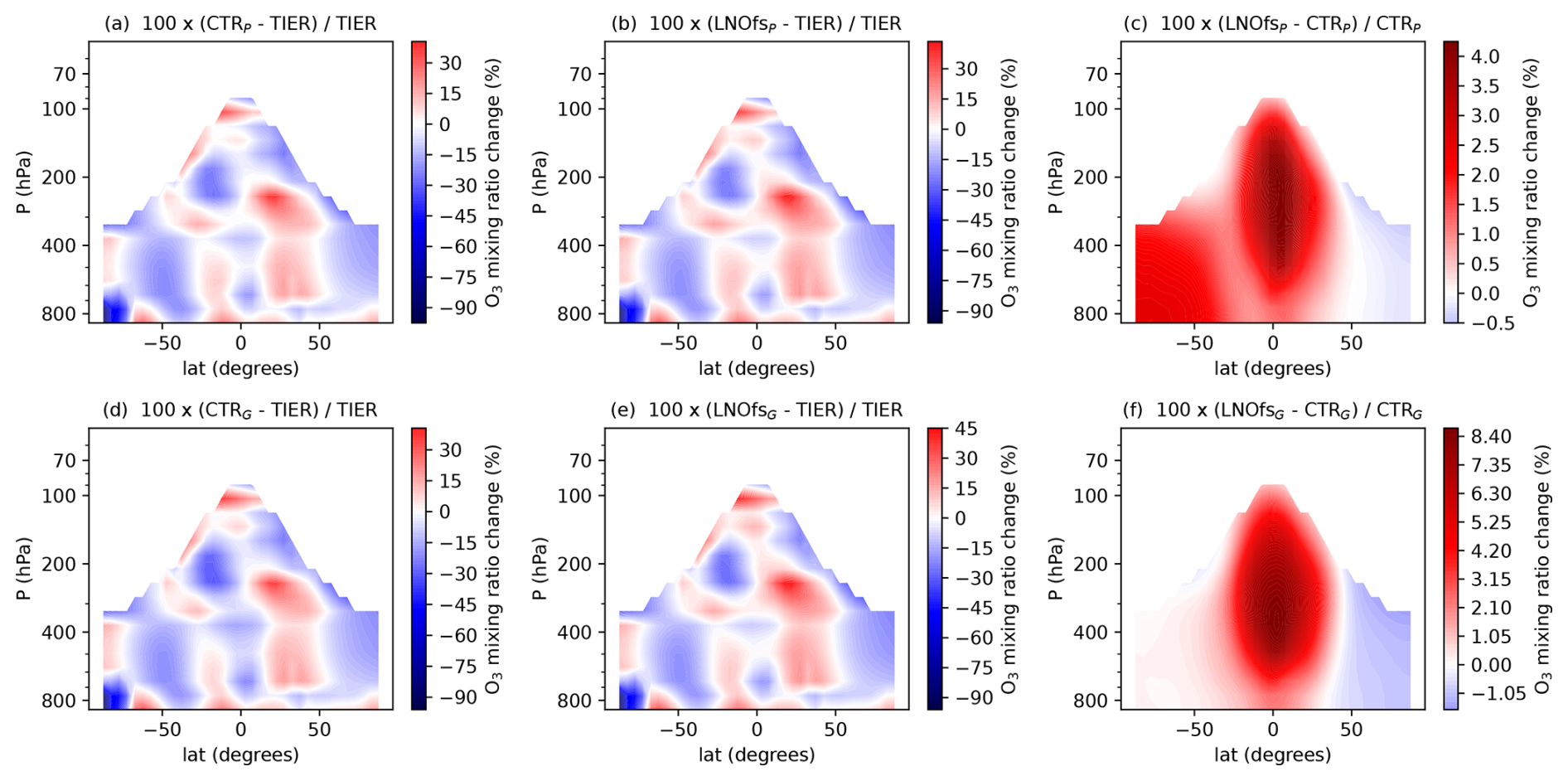
Figure 14 Seasonally (September–October–November, SON) and zonally averaged differences (in %) in the vertical O₃ mixing ratio between the simulations and the Bodeker Scientific global vertically resolved ozone database Tier 1.4 vn1.0 product Hassler et al. (2009). The border with the white region represents the zonally averaged mean altitude of the climatological tropopause. The subscript indicates the lightning parameterization: P represents Price and Rind (1992) and G represents Grewe et al. (2001).

The seasonal variations in the simulated zonal ozone distribution between 2002 and 2007 (Figs. 11–14) can be compared with the corresponding interannual zonally averaged differences in the vertical O₃ mixing ratio provided by the Bodeker Scientific global vertically resolved ozone database (Tier 1.4, version 1.0) (Hassler et al., 2009). These differences, calculated relative to the seasonal mean for 2002–2007, are shown in Figs. S26–S29. This comparison aims to evaluate the significance of the observed variations. The seasonal variations between the simulated tropospheric O₃ and the Tier 1.4 product are most pronounced in the tropics and the middle troposphere (Figs. 11–14), whereas the interannual variations in the Tier 1.4 product peak in the extratropics and the upper troposphere (Figs. S26–S29). Consequently, we conclude that the differences in tropospheric O₃ between the simulation and the Tier 1.4 product are relevant, since they exceed the interannual variability of tropospheric O₃.

The interannual zonally averaged differences during each season of the vertical O₃ mixing ratio between the annual Bodeker Scientific global vertically resolved ozone database Tier 1.4 vn1.0 product (Hassler et al., 2009) and the annual mean during the period 2002–2007 for each season are shown in Figs. S26–S29.

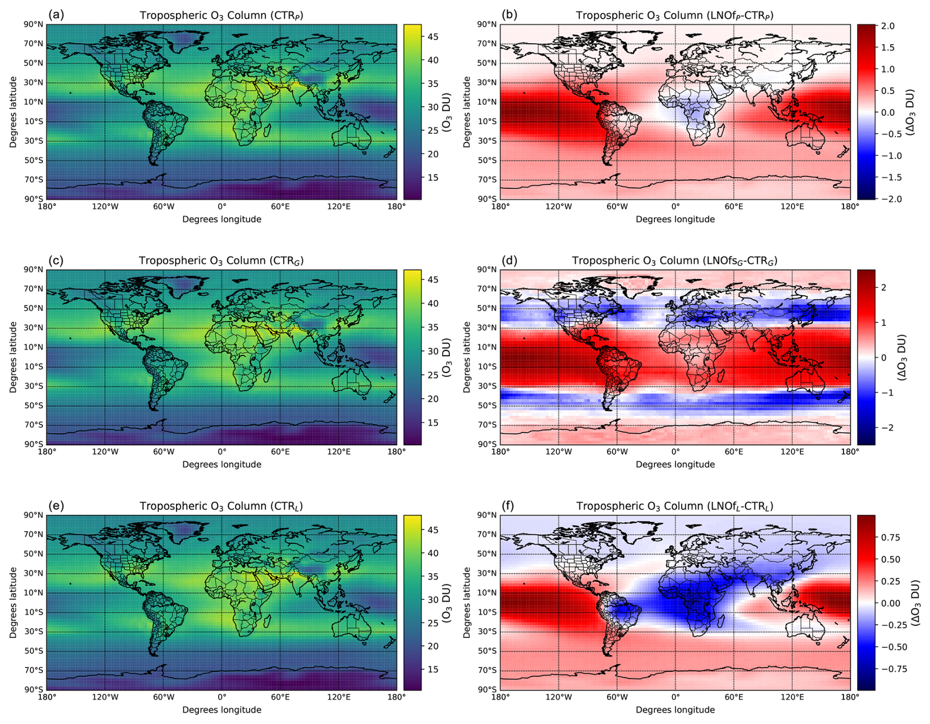
Figure 15 Annually (2002–2007) and globally averaged tropospheric column of O₃ in the CTR simulations (a, c, and e) and differences in the O₃ total column (integrated between the ground and the top of the troposphere) between the LNOfs and CTR simulations (b, d, and f). The values are given in Dobson Units (DU). The subscript indicates the lightning parameterization: P represents Price and Rind (1992), G represents Grewe et al. (2001), and L represents Luhar et al. (2021) (see Table 1). The monthly total O₃ column from the CTR_G simulation can be seen in Figs. S14–S25.

Jöckel et al. (2016, Fig. 29) compared the annual tropospheric partial column of ozone from the RC1-base-07 simulation with AURA Microwave Limb Sounder/Ozone Monitoring Instrument (MLS/OMI; Ziemke et al., 2011) measurements (reproduced in Fig. S30), obtaining an overestimation of ozone in the tropics, especially over Africa, Indonesia, and the Indian Ocean. In turn, the RC1-base-07 simulation produced an underestimation of the tropospheric partial column of ozone below about 50° S latitude. We show in Fig. 15 a comparison of the annual-averaged tropospheric partial column of ozone between the CTR and LNOfs simulations. The LNOfs simulations with the parameterizations based on the CTH (LNOfs_P and LNOfs_L) produce a smaller tropospheric column of ozone in tropical Africa compared to the CTR parameterizations, resulting in a better agreement with measurements (Jöckel et al., 2016, Fig. 29). In turn, LNOfs_P and LNOfs_L produce a larger column of tropospheric ozone below 50° S latitude than the CTR simulations, leading to a better agreement with measurements. The LNOfs_L simulation results in a smaller column of tropospheric ozone above 50° N latitude, showing again a better agreement with observations. However, the obtained overestimation of tropospheric ozone over the tropical oceans disagrees more with the measurements. In the case of the G simulations, the LNOfs_G simulation produces a better agreement with measurements above 30° N latitude than the CTR_G simulation but less agreement over the rest of the globe.

3.4 Limitations and uncertainties

In this study, we examine the impact on atmospheric chemistry of parameterizing LNO_x production based on lightning frequency. In particular, we use the global relationship between LNO_x production and flash frequency as derived by Bucsela et al. (2019, Fig. 11c). While substantial evidence exists, suggesting possible relationships between LNO_x production per flash and flash frequency (Bucsela et al., 2019; Allen et al., 2019, 2021; Zhang et al., 2022; Pérez-Invernón et al., 2023b; Pickering et al., 2024), quantifying this relationship on a global scale using satellite-based data and global lightning measurements remains challenging and uncertain, as discussed by Bucsela et al. (2019). Firstly, it is important to emphasize that the relationship provided by Bucsela et al. (2019) was derived over midlatitude land regions, but it is applied globally in this study. However, Allen et al. (2019) used a similar method to derive LNO_x PE within the tropics (including oceans), finding that tropical PE is only 10 % lower than the midlatitude PE derived by Bucsela et al. (2019). In addition, Allen et al. (2019) reported evidence for a decrease in LNO_x PE with increasing flash rate on a regional basis within the tropics.

The low detection efficiency of WWLLN in some regions (Holzworth et al., 2009) together with the uncertainty in satellite-based vertical column density of NO_x introduce a large uncertainty in the estimated LNO_x production. Bucsela et al. (2021) used TROPOMI NO₂ and cloud measurements together with GLM lightning data to improve the estimation of LNO_x production. They reported that the relationship between the production of LNO_x per flash and the flash frequency for thunderstorms producing less than 3000 flashes per hour and degree in America (98 % of all the analysed cases) could be weaker than the relationship reported by Bucsela et al. (2019). Therefore, the results obtained in this study should be regarded as the upper limit of the impact that an LNO_x production parameterization based on lightning flash frequency may have on the chemical composition of the atmosphere.

4 Conclusions

For the first time, a parameterization of LNO_x production, based on the flash frequency, is introduced in the climate–chemistry model EMAC. This LNO_x parameterization is based on OMI NO₂ measurements provided by Bucsela et al. (2019), who reported an inverse relationship between the lightning flash frequency in thunderstorms and the production of LNO_x per flash. Although more recent studies have reported a weaker relationship between the production of LNO_x per flash and the flash frequency in America (Bucsela et al., 2021), there are no new estimates of this relationship on a global scale. Therefore, the results obtained in this study should be considered the upper limit of the impact that an LNO_x production parameterization based on lightning flash frequency could have on atmospheric chemical composition. Three pairs of 8-year simulations by using three different lightning parameterizations (Price and Rind, 1992; Grewe et al., 2001; Luhar et al., 2021) enable us to investigate the influence of this LNO_x production parameterization for the mixing ratios of NO_x = NO + NO₂, O₃, CO, HO_x = H + OH + HO₂, N₂O, HNO₃, and HNO₄ in the troposphere.

Based on our findings, the LNO_x production parameterization based on the lightning flash frequency leads to an enhanced production of LNO_x in thunderstorms with lower flash rates compared to those that impose a constant LNO_x production rate per flash. This increase in LNO_x production in weaker thunderstorms results in less LNO_x over land and more over the oceans. In turn, more LNO_x is emitted in winter thunderstorms than in summer thunderstorms. In general, the simulations with the new parameterization of the LNO_x production lead to a spatial distribution of LNO_x that is more homogeneously distributed over the globe than the simulations with a constant LNO_x production per flash (Fig. 3). As a result, we obtain a larger tropospheric column of ozone over the tropical ocean (Figs. 6–9). The influence of the new LNO_x production parameterization on tropospheric ozone in other regions of the globe depends on the employed lightning flash frequency parameterization. For the lightning flash frequency parameterizations based on the CTH (Price and Rind, 1992; Luhar et al., 2021), we obtain a smaller tropospheric column of ozone over tropical Africa. In the case of the lightning parameterization based on the upward flux of mass (Grewe et al., 2001), we obtain a smaller column of tropospheric ozone at midlatitudes in the Northern Hemisphere. The maximum change of the tropospheric ozone mixing ratio when using the new scheme is of the order of ∼ 3 %, with the lowest variations in the case of the lightning parameterization by Luhar et al. (2021), which already included a modification of lightning frequency over oceans.

The oxidation capacity of the atmosphere is influenced by the new LNO_x production parameterization, as tropospheric NO_x plays an important role in the chemical budget of tropospheric HO_x. In particular, we obtain a global decrease in the tropospheric lifetime of methane with respect to OH ranging between 0.7 % and 3.4 %, especially over the Southern Hemisphere.

The new parameterization of the production of LNO_x leads to a decrease in tropospheric CO by about 2 % worldwide, reaching its maximum over the tropical oceans. The mixing ratio of tropospheric HNO₃ is reduced up to 8 % globally, especially over land. Finally, we obtain an increase in the tropospheric HNO₄ mixing ratio of about 4 %, with significant increases over ocean and decreases over land.

These findings highlight the importance of understanding the variability of LNO_x production to enhance the chemical budget of key trace gas species in climate–chemistry models. Geostationary satellite measurements of NO₂ have the potential to significantly contribute to more accurate LNO_x production parameterizations. Examples of such satellites include the Geostationary Environment Monitoring Spectrometer (GEMS, launched in February 2020; Kim et al., 2020), the Tropospheric Emissions: Monitoring of Pollution (TEMPO, launched in April 2023; Zoogman et al., 2017), and the Meteosat Third Generation (MTG) imaging and sounding satellites (Holmlund et al., 2021). In particular, continuous (1 hourly) measurements of NO₂ provided by geostationary satellites over an area can offer unprecedented insight into the temporal evolution of LNO_x in thunderstorms at a quasi-global scale, revealing the relationships between LNO_x production per flash and thunderstorm evolution.