Surface temperature effects of recent reductions in shipping SO₂ emissions are within internal variability

In 2020, the International Maritime Organization (IMO) implemented strict new regulations on the emissions of sulfate aerosol from the world's shipping fleet. This can be expected to lead to a reduction in aerosol-driven cooling, unmasking a portion of greenhouse gas warming. The magnitude of the effect is uncertain, however, due to the large remaining uncertainties in the climate response to aerosols. Here, we investigate this question using an 18-member ensemble of fully coupled climate simulations evenly sampling key modes of climate variability with the NCAR model, the Community Earth System Model version 2 (CESM2). We show that, while there is a clear physical response of the climate system to the IMO regulations, including a surface temperature increase, we do not find global mean temperature influence that is significantly different from zero. The 20-year average global mean warming for 2020–2040 is +0.03 °C, with a 5 %–95 % confidence range of [$-\mathrm{0.09},\mathrm{0.19}$], reflecting the weakness of the perturbation relative to internal variability. We do, however, find a robust, non-zero regional temperature response in part of the North Atlantic. We also find that the maximum annual mean and ensemble mean warming occurs around 1 decade after the perturbation in 2029, which means that the IMO regulations have likely had very limited influence on observed global warming to date. We further discuss our results in light of other, recent publications that have reached different conclusions. Overall, while the IMO regulations may contribute up to 0.16 °C [$-\mathrm{0.17},\mathrm{0.52}$] to the global mean surface temperature in individual years during this decade, consistent with some early studies, such a response is unlikely to have been discernible above internal variability by the end of 2023 and is in fact consistent with zero throughout the 2020–2040 period.

1 Introduction

Anthropogenic aerosols play a complex and dual role in Earth's climate system. On the one hand, they contribute to atmospheric pollution, adversely affecting air quality and public health. On the other hand, they mostly exert a net cooling effect on the climate by increasing the albedo, or reflectivity, of the atmosphere, thereby reducing the amount of solar radiation that reaches the Earth's surface (Bellouin et al., 2020). Sulfate aerosols, for instance, scatter sunlight directly and enhance cloud brightness by increasing the number of water droplets in clouds, further reflecting sunlight away from the Earth (e.g. Albrecht, 1989; Twomey, 1974). Anthropogenic aerosol emissions thereby currently induce a global average cooling which (partially) offsets greenhouse-gas-driven warming by around 0.5 [0.22–0.96] °C compared to pre-industrial times (Forster et al., 2021). The magnitude of aerosol cooling is a key uncertainty in climate science and hinders our ability to accurately predict the magnitude and timing of future warming (Watson-Parris and Smith, 2022).

Environmental and health concerns associated with anthropogenic aerosols have led to international efforts to reduce their emission, with potentially significant consequences for the climate (Wall et al., 2022). In January 2020, the International Maritime Organization (IMO) took a significant step in this direction by implementing stringent regulations to curb sulfur dioxide (SO₂; a precursor for sulfate aerosol) emissions from the global shipping fleet (IMO 2019), which at the time contributed around 14 % of all anthropogenic sources of these pollutants (Christensen et al., 2022). Given the substantial share of global trade transported by sea, and the corresponding volume of emissions from shipping, the impact of these regulations on the global climate system was anticipated to be notable and to provide a useful experiment to quantify broader aerosol impacts (Christensen et al., 2022). Similar regulatory efforts in other sectors, and national efforts in major industrial nations such as China (Li et al., 2017; Samset et al., 2019; van der A et al., 2017), also aim to improve air quality by reducing emissions of SO₂ and other aerosol precursors or species, thereby posing a challenge to climate scientists: to quantify and predict how these reductions will influence Earth's energy balance and the ongoing rate and pattern of warming.

While focused studies have found evidence of the effect of the change in shipping emissions on cloud brightness (Diamond, 2023; Watson-Parris et al., 2022), it is challenging to discern any signal in large-scale cloud properties because the observed covariability does not always flow causally from the observed microphysical properties (Glassmeier et al., 2021; Stevens and Feingold, 2009). The instantaneous radiative forcing due to aerosol–cloud interactions from the 2020 change in shipping emissions is estimated to be 0.5 W m⁻² in the annual mean within shipping corridors (Diamond, 2023). Best estimates of the global mean effective radiative forcing (ERF) resulting from an 80 % drop in shipping emissions range from 0.035 to 0.15 W m⁻² across multiple models and methodologies (Gettelman et al., 2024; Skeie et al., 2024; Yoshioka et al., 2024). Yuan et al. (2024) report a forcing of 0.2 W m⁻² averaged over the global ocean only, which is consistent with these global estimates.

A possible discernible climate influence of the IMO regulations became a topic for discussion in 2023, when observed global mean surface temperatures (GMSTs) set a record. The 2023 GMST anomaly exceeded predictions based on long-term climate change trends and internal variability, including the El Niño–Southern Oscillation (ENSO), by more than 0.2 °C, causing speculation that the reduction in SO₂ emissions from shipping could be one of the driving factors (Schmidt, 2024). Based on the estimates of ERF given above, however, calculations with simple energy balance models (EBMs) suggest that the warming associated with shipping changes since 2020 is unlikely to exceed 0.05 °C by 2023, with a long-term response of 0.07 °C (Gettelman et al., 2024). A weakness of the EBMs in this case, however, is that they generally assume a spatially homogeneous forcing and thus cannot account for the spatial heterogeneity in ocean feedbacks or climate responses to aerosol forcing, which is known to be substantial (Persad and Caldeira, 2018; Shindell et al., 2009; Westervelt et al., 2020).

To provide a quantitative estimate of the magnitude and pattern of the climate response to the IMO shipping regulations, and the role it may have played in recent record surface temperatures, it is therefore crucial to also have estimates using fully coupled Earth system models (ESMs) that take into account a broad range of aerosol–climate interactions and their spatial heterogeneity, along with internal variability and its potential feedback on transient climate forcing. The latter means that it is necessary to use an ensemble of model simulations that is sufficiently large to discern a statistically significant temperature response to a weak perturbation. Even with ESMs, structural uncertainty and ensemble size create disagreement, as evidenced by recent studies of surface warming estimates due to shipping emission reductions. For instance, Yoshioka et al. (2024) found a global mean temperature increase of 0.04 °C, averaged over 2020 to 2049, in response to a 0.13 W m⁻² ERF in HadGEM3-GC3.1, while Quaglia and Visioni (2024) found a global temperature increase of 0.2 °C by 2030 in response to an approximately 0.2 W m⁻² radiative perturbation in the Community Earth System Model version 2 (CESM2; for a 90 % reduction in shipping emissions).

Here, we present estimates of the transient surface temperature implications of the recent IMO regulations, using a large (18-member) ensemble of fully coupled transient simulations with CESM2. We show the ensemble mean response over time and discuss the implications of the sample size for the ability to quantify any forced warming. Also, as it is conceivable that the current specific phases of ENSO and the Atlantic Multi-decadal Oscillation (AMO) could be particularly (in)sensitive to radiative perturbations in the shipping corridors (e.g. Wang et al., 2022), we have designed the ensemble to sample different modes of climate variability. Finally, as there have already been a range of studies quantifying the temperature response to the IMO regulations leading to differing, if not opposite, conclusions, we provide a broader discussion on the challenges and limitations of disentangling the effect of shipping emissions using currently available climate modelling methodologies.

2 Methods

CESM2 (Danabasoglu et al., 2020) consists of the Community Atmosphere Model version 6 (CAM6; Bogenschutz et al., 2018), the Parallel Ocean Program version 2 (POP2; Danabasoglu et al., 2012), the Community Land Model version 5 (CLM5; Lawrence et al., 2019), and the Community Ice Code version 5 (CICE; Hunke et al., 2013). Aerosols in CAM6 are represented by the four-mode version of the Modal Aerosol Module (MAM4; Liu et al., 2016). We note that 2.5 % of SO₂ emissions from the international shipping sector are emitted as sulfate aerosol at the surface level and into the accumulation mode (Emmons et al., 2020). The cloud microphysics scheme is version 2 of the Morrison–Gettelman scheme (Gettelman and Morrison, 2015). Simulations are performed at approximately 1° horizontal resolution.

Our baseline experiments come from archived simulations performed as part of the CESM2 Large Ensemble (CESM2-LE) project (Rodgers et al., 2021). From 2015 onwards, CESM2-LE uses aerosol/precursor gas emissions (including ${\mathrm{SO}}_{\mathrm{2}}/{\mathrm{SO}}_{\mathrm{4}}$ from international shipping), land use changes, and greenhouse gas concentrations from the Shared Socioeconomic Pathway 3-7.0 (SSP3-7.0; O'Neill et al., 2016). Our perturbation experiments are initialised from the CESM2-LE baseline experiments beginning in 2015 and integrated through 2040. The perturbation simulations are identical to the baseline simulations, except for a uniform 80 % reduction in ${\mathrm{SO}}_{\mathrm{2}}/{\mathrm{SO}}_{\mathrm{4}}$ emissions from international shipping starting in 2020 (consistent with the IMO regulations) and extending through 2040. Thus, taking a difference (perturbation minus baseline) isolates the effects of the decrease in SO₂ emissions from international shipping.

CESM2 has a relatively strong anthropogenic aerosol forcing when quantified in isolation and a high climate sensitivity compared to other ESMs (see Fig. 1; Schlund et al., 2020; Zelinka et al., 2023). Its oceanic response has also been shown to be particularly sensitive to aerosol emissions (Fasullo et al., 2023; Hassan et al., 2021). For this particular perturbation, however, CESM2 shows a similar radiative forcing to other ESMs (Skeie et al., 2024). Our model setup is the same as the one used for CESM2 in Gettelman et al., 2024, who report an ERF of 0.11 W m⁻² for a 100 %±25 % reduction in shipping SO₂ emissions. This places CESM2 near the mean of the ERF estimates recently provided (Skeie et al., 2024; Gettelman et al., 2024).

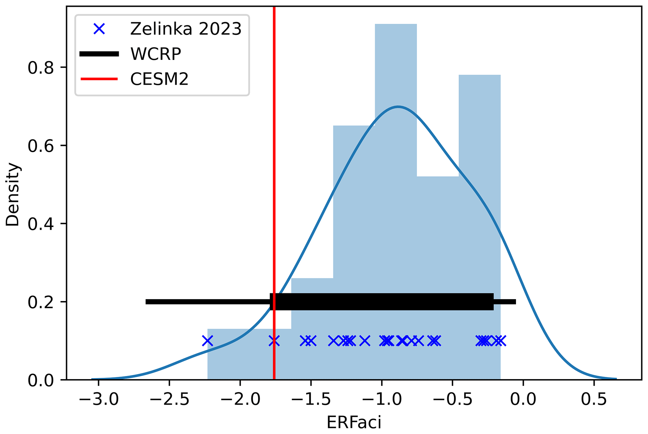
Figure 1 Distribution of the effective radiative forcing due to aerosol–cloud interactions (ERFaci) in CMIP6 models as assessed by Zelinka et al. (2023) in blue and Bellouin et al. (2020) in black, with CESM2 highlighted in red.

To help understand the possible importance of the imposed shipping emission perturbation relative to internal climate variability, we perform 18 ensemble simulations. These ensemble members all use CESM2-LE realisations that feature 11-year running mean smoothed CMIP6 biomass burning emissions, including members 1011-001, 1031-002, 1051-003, 1091-005, 1111-006, 1131-007, 1151-008, 1171-009, 1191-010, 1231-011, 1231-012, 1231-016, 1231-018, 1251-012, 1281-017, 1281-020, 1301-015, and 1301-017. All comparisons and differences are calculated with respect to the 18 corresponding unperturbed ensemble members. Recent satellite data introduce more interannual variability into the biomass burning dataset than data sources used before 1997 and after 2014, so smoothing reduces the variability in biomass burning fluxes over 1990–2020 (Fasullo et al., 2022). Furthermore, to help understand the possible importance of dominant modes of climate variability (e.g. ENSO and AMV) to the climate impacts associated with the shipping perturbation, 8 of the above ensemble members feature ENSO-neutral conditions, 5 feature ENSO-positive conditions, and 5 feature ENSO-negative conditions. The AMV index is also evenly sampled in the ensemble, for each ENSO state, and spans −0.15 to 0.15.

The simulated responses are compared to observed SST changes, diagnosed from the HadCRUT v5.0.2 analysis (Morice et al., 2021). We fit a locally weighted regression (LOESS) model over time to each 5°×5° grid cell to model the long-term SST trends (2020–2040) and then subtract this to discern the anomaly in 2023.

In the following, unless otherwise specified, estimates for surface temperature change are for the period 2020–2040. All significance tests are performed using a two-sided Student's t-test for the null hypothesis that two independent samples (drawn from two distributions with equal variance) have identical average (expected) values.

3 Results

Figure 2a shows the relative change in near-surface SO₂ concentration in the reduction scenario compared to baseline and demonstrates that the majority of the changes in near-surface SO₂ occur over the Northern Hemisphere oceans and in particular over the North Atlantic and northeastern Pacific – clearly aligned with the main international shipping routes. Figure 2b shows the change in near-surface SO₂ concentrations over the simulation period both globally and over the North Atlantic. The gradual reduction in the change over the period is due to the underlying shipping emission reductions in the baseline SSP3-7.0 scenario.

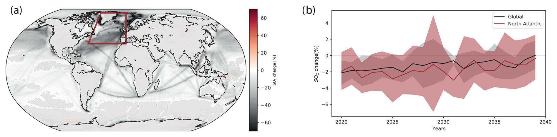
Figure 2 (a) Relative change in SO₂ near the surface due to the shipping emission perturbation, averaged over the whole 2020–2040 period, where stippling represents locations where the null hypothesis of “no change” cannot be rejected at P<0.05. (b) Annual mean evolution of SO₂, averaged over the entire globe (black line; shading shows ±1 standard deviation in ensemble member spread) and over the North Atlantic region (red line), as indicated on the map. All changes are relative to the baseline Shared Socioeconomic Pathway 3-7.0 (SSP3-7.0).

Despite these widespread and regionally significant changes in SO₂ concentrations (and corresponding SO₄ concentrations, not shown), the temperature response in these simulations is negligible. Based on our sample of 18 simulations, we calculate a global 20-year mean surface temperature change from the IMO regulations of +0.03 °C, with a 5 %–95 % confidence range of [$-\mathrm{0.09},\mathrm{0.19}$]. Figure 3a shows the temperature change with respect to the baseline simulations as a global mean and over the North Atlantic, neither of which show significant spatial mean warming over the 20-year study period. In fact, over the first 5 years, there is no statistically robust change in temperature found anywhere on the globe (see Fig. 3b), demonstrating the low strength of the perturbation with respect to the model's simulated internal variability in the Earth system. Averaging over 20 years, a robust localised signal starts to appear during 2020–2040 in a small region of the North Atlantic (see Fig. 3c) where there is a statistically significant local warming of around 0.2 °C. Figure 3d shows that the anomalous warming observed in the region in 2023 (see Methods) does broadly correspond with the pattern of simulated warming in response to the IMO regulations but only as discerned after 20 years, visualised in Fig. 3e (which is a close-up of Fig. 3c).

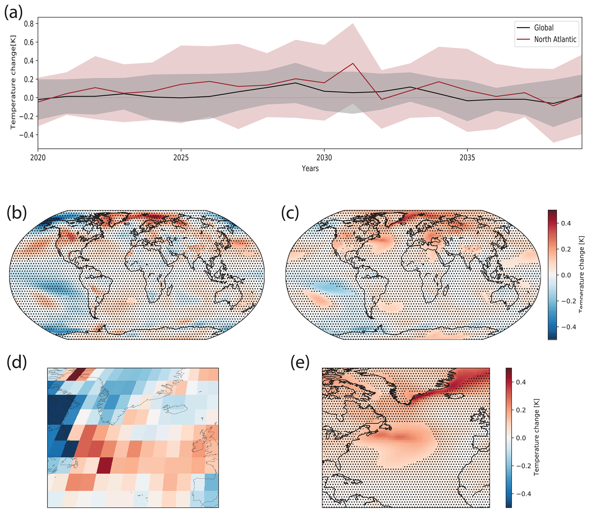
Figure 3 (a) Global and North Atlantic annual mean evolution in temperature change (shading shows ±1 standard deviation in ensemble member spread). (b) Annual mean temperature change for 2020–2025. (c) Annual mean temperature change for 2020–2040. (d) Observed anomalous warming in North Atlantic sea-surface temperature in 2023. (e) A close-up of panel (c) showing the corresponding region of the North Atlantic. Stippling in panels (b), (c), and (e) represents locations where the null hypothesis of “no change” cannot be rejected at P<0.05. All changes are relative to the corresponding baseline CESM2 LENS simulations of SSP3-7.0.

Despite some degree of similarity between the recent observed anomalous warming and the simulated temperatures shown in Fig. 3e, the timescales do not match. The observed anomalies occurred 3 years after the emissions changes, while the average model response over the first 5 years (2020–2025) shows no significant warming in the region (Fig. 3b). As noted above, it is possible that the particular phase of ENSO or AMO could have made the North Atlantic particularly susceptible to such a perturbation in this short period of time in observations, but, by sub-sampling our ensemble based on these characteristic modes, we still find no evidence that the shipping emission changes could have contributed significantly to the observed global temperature changes (see Fig. 4).

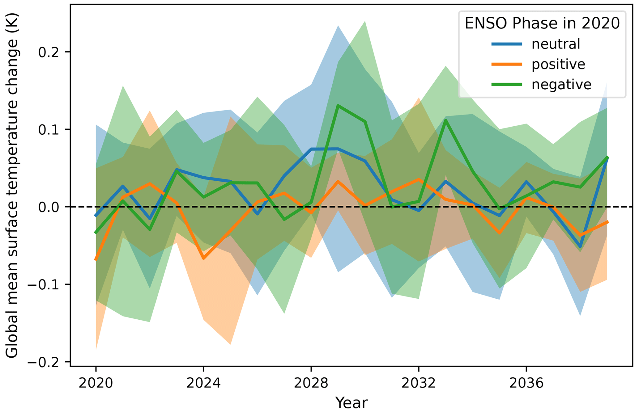
Figure 4 Global mean change in surface temperature due to shipping emission changes with respect to the baseline SSP3-7.0 simulations, subdivided into three ENSO phases in 2020: neutral (blue; 8 members), positive (orange; 5 members), and negative (green; 5 members). Shading shows the inter-member spread, represented by ±1 standard deviation.

As mentioned above, detecting the climate impacts of a relatively small externally forced perturbation, such as the estimated global top-of-atmosphere radiative forcing associated with the IMO shipping regulations (e.g. $+\mathrm{0.12}\pm \mathrm{0.03}\mathrm{W}{\mathrm{m}}^{-\mathrm{2}}$; Gettelman et al., 2024), is complicated by the influence of internal climate variability (Deser et al., 2012, 2020). Figure 5 shows the actual evolution of our 18 ensemble members, with and without the IMO regulations, compared to the HadCRUT5 global surface temperature anomaly data series. The observed evolution is clearly within the range sampled by CESM2, in both emission scenarios. This difficulty is compounded over smaller (e.g. regional) spatial scales and shorter (e.g. decadal) timescales. The ability to robustly separate and quantify a forced signal in the climate system is the goal and motivation of large ensembles (e.g. Kay et al., 2015; Kirchmeier-Young et al., 2016; Maher et al., 2019; Rodgers et al., 2021; Simpson et al., 2023), whereby dozens or more independent climate model ensemble members are generated using identical external forcing but different initial climate states. Since ensemble members will in general feature different timing of internal climate variability, which essentially represents noise (i.e. the component of the signal that is not externally forced), averaging over a larger number of ensemble members reduces such noise, allowing a more robust quantification of the externally forced signal.

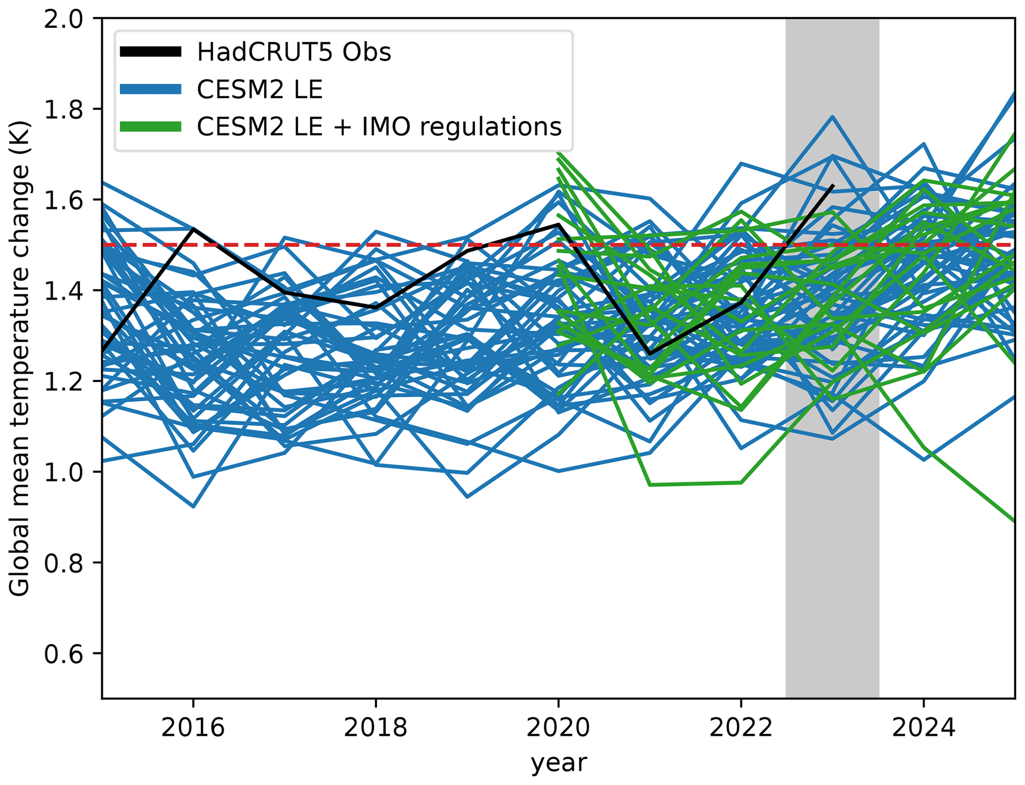
Figure 5 Global mean surface temperature change with respect to piControl for the baseline historical + SSP3-7.0 CESM2 LENS ensemble (blue) and the perturbed shipping emission ensemble performed in this study (green), overlaid on the HadCRUT SST observational estimate (with respect to the 1850–1900 average; black). The year 2023 is highlighted. The dashed red line represents the 1.5 °C Paris Agreement warming threshold.

Figure 6 shows the important influence of internal climate variability on the global mean temperature response (dT) in our CESM2 shipping perturbation experiments and the importance of having a sufficient ensemble size to robustly detect a forced response. Figure 6a shows the impact of randomly selecting N of our 18 ensemble members with replacement (i.e. a bootstrapping analysis). For each combination, we calculate the corresponding ensemble global mean temperature response. The figure shows the results for N=1000 samples. For small N, the spread in the ensemble mean ΔT is quite large (approximately −0.09 to 0.125 °C for N=5). For N=10, the spread is reduced, but it still exceeds ±0.05 °C. As N continues to increase, however, the spread converges to our 18-ensemble-member ΔT.

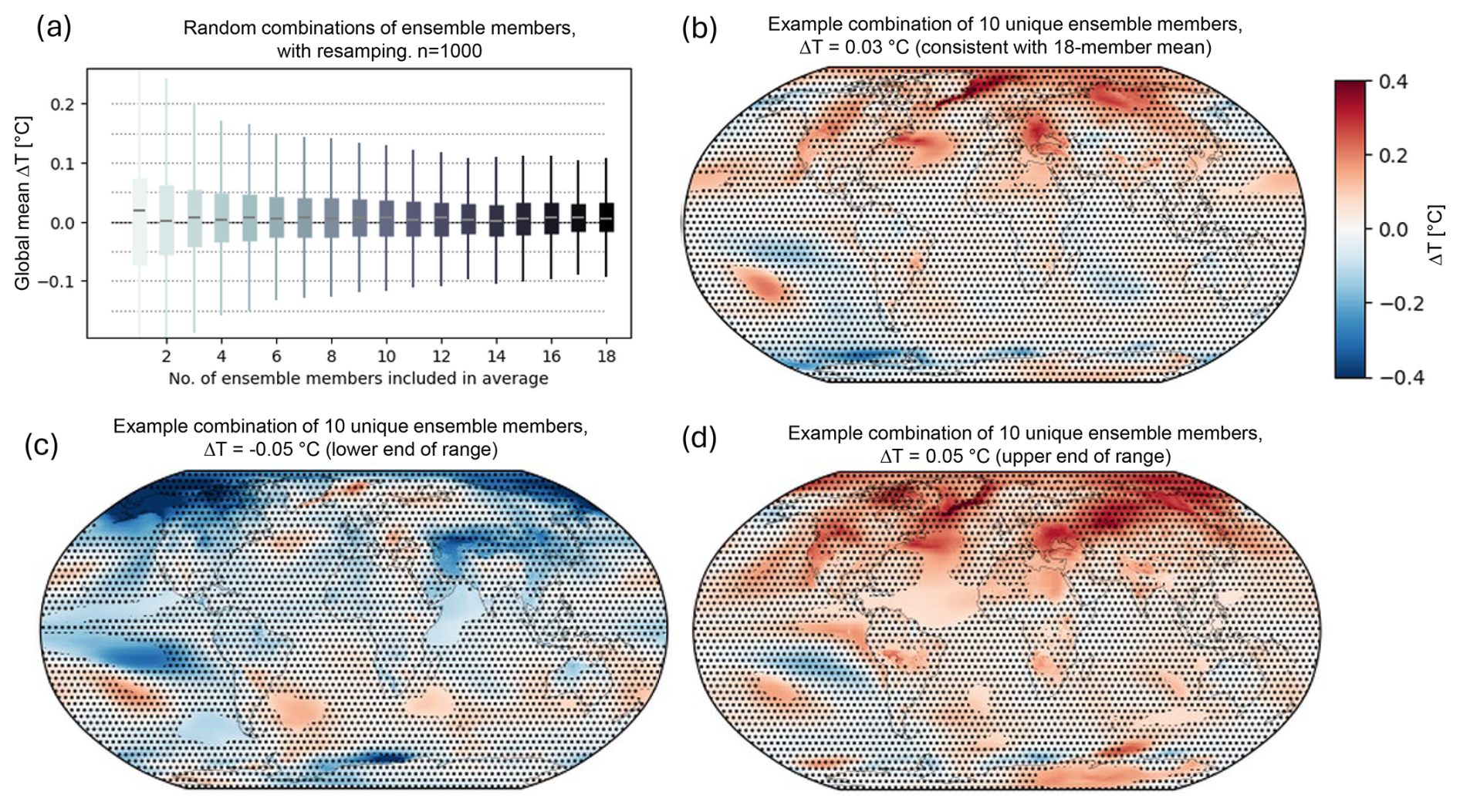
Figure 6 Ensemble size is crucial for quantifying a forced signal for weak perturbations. (a) Spread in the 2020–2040 global annual mean surface temperature change (ΔT) when randomly sampling and averaging N (given on the x axis) ensemble members out of a total of 18 available members 1000 times, with resampling. Each spread includes 1000 combinations, illustrating an increasing robustness of ΔT with the number of ensemble members. Boxes show the median and 5 %–95 % range, and whiskers show the maximum and minimum values. (b) Example combination of 10 ensemble members, where the global annual mean ΔT is consistent with the 18-member mean (ΔT=0.03 °C). Hatching shows grid points not significant at the 95 % confidence level, as for Fig. 2. (c) Same as panel (b) but for an example combination consistent with ΔT at the lower end of the 10-member mean range. ($\mathrm{\Delta }T=-\mathrm{0.05}\mathrm{°}\mathrm{C}$). (d) Same as panel (b) but for an example combination consistent with ΔT at the upper end of the 10-member mean range. (ΔT=0.05 °C).

To further illustrate the importance of ensemble size when dealing with perturbations that have weak responses relative to internal variability, Fig. 6b–d show example combinations of 10 unique ensemble members (as used, for example, by Quaglia and Visioni, 2024). Statistical testing and hatching is done as for our Fig. 3 (see Methods). Figure 6b shows a 10-member combination consistent with our 18-member mean response (ΔT=0.03 °C). Figure 6c and d show 10-member combinations with ΔT at the edges of, but still within, the 9 %–95 % confidence interval ($\mathrm{\Delta }T=\pm \mathrm{0.05}\mathrm{°}\mathrm{C}$).

While panels b–d of Fig. 6 all represent deliberate picking of ensemble members, the analysis illustrates how, even with a decently sized ensemble of 10 members, one could conclude that the IMO shipping regulations may lead to substantial global mean warming or global mean cooling. This illustrates the importance of internal climate variability in detecting a global mean temperature response associated with the IMO shipping regulations and the importance of a sufficiently large ensemble size to reduce the risk of spurious conclusions. We note that our choice of 18 ensemble members, as with most experimental designs, also represents a trade-off between additional information gained versus increased computational expense. Clearly, however, a moderately large ensemble size of 10, which has been shown to be sufficient in some contexts (e.g. Monerie et al., 2022), is not sufficient to make robust claims regarding the impact of shipping SO₂ reductions on global mean temperature, in particular during its early transient evolution.

4 Discussion and conclusions

The strict new fuel regulations introduced by the IMO provided a valuable experiment to better understand the role of changing anthropogenic aerosol in the climate system, particularly as an analogue to other, current and future, efforts to improve air quality globally. Using an 18-member ensemble of simulations from CESM2, we find that the global temperature response to the IMO regulations that came into force in 2020 is +0.03 °C, with a 5 %–95 % confidence range of [$-\mathrm{0.09},\mathrm{0.19}$] for the period 2020–2040. This result, which is consistent with a null hypothesis of no discernible global mean temperature response, is at the low end of other estimates of this warming effect, from simple energy balance models (Gettelman et al., 2024; Yuan et al., 2024) and global climate models (Quaglia and Visioni, 2024; Yoshioka et al., 2024), which suggested global warming between 0.04 °C (Yoshioka et al., 2024) and 0.2 °C (Quaglia and Visioni, 2024) associated with the shipping regulations over decadal timescales. To understand the differences between these conclusions and to explain why our analysis provides an important bound on the role of shipping emission changes in recently observed temperature extremes, it is necessary to discuss in some detail the methodologies and framings behind the other results.

Some recent studies of the climate impact of the IMO regulations used EBMs to calculate the global temperature response from the effective radiative forcing (Gettelman et al., 2024; Yuan et al., 2024). These simple models are useful in many situations, notably for comparing the climate implications of known emissions from industrial sectors, regions, or scenarios. However, for absolute climate impacts, they require substantial assumptions to be made about the sensitivity and timescale of the responses, and critically do not account for regional heterogeneity of responses or climate feedbacks, such as influences on ocean circulation or sea ice, or of internal variability. Ocean feedbacks may be particularly important in the case of shipping emission changes which are focused over the Northern Hemisphere oceans, where it is conceivable that the ocean mixed layers may warm more efficiently than, for example, the Southern Ocean (e.g. Ma et al., 2020). Region-specific cloud responses and teleconnections to aerosol changes over Northern Hemisphere oceans may also differ from those to, for example, sulfur emission changes in Asia (Burney et al., 2022; Persad and Caldeira, 2018), which tend to dominate the total global response to recent sulfur emission changes used to calibrate simple EBMs. Coupled climate models provide estimates of the temperature response to the IMO regulations that take such feedbacks and pattern dependencies into account.

Despite the differences in the approach, our estimate of the global warming due to the IMO regulations is similar to the estimate by Gettelman et al. (2024) of 0.07 °C by 2030, which is based on the FaIR EBM. The EBM approach taken by Yuan et al. (2024), however, which diagnoses a global temperature anomaly of 0.17 °C at equilibrium, overstates the response to their forcing by a factor of 1.4. This is because Yuan et al. (2024) calculate a global temperature response using a global climate feedback parameter but also using an ocean area mean ERF. A global feedback parameter should be used with a global forcing in this context, which would reduce their forcing and temperature estimates by a factor of 0.7, the fraction of global area that is ocean, from 0.2 to 0.14 W m⁻² and 0.17 to 0.12 °C in equilibrium, respectively. Uncertainty in the climate feedback parameter should also be considered in this estimate. Using a feedback parameter equivalent to that of CO₂, the AR6 likely range for ECS of 2.5–4.0 °C (which may both be overly simplistic assumptions) and 2×CO₂ forcing of $\mathrm{3.9}\pm \mathrm{0.5}\mathrm{W}{\mathrm{m}}^{-\mathrm{2}}$ (90 % range) would produce an equilibrium warming due to a forcing of 0.14 W m⁻² of 0.09–0.14 °C (90 % range). Altogether, 7 years, the timescale used by Yuan et al. (2024) in their calculation, is approximately the time taken for the upper ocean to reach equilibrium, so, based on Gregory et al. (2024), one would expect to see around two-thirds of the equilibrium response (i.e. 0.06–0.10 °C) in that time. With these factors taken into account, the estimates presented by Yuan et al. (2024) would have been consistent with those of Gettelman et al. (2024) and those presented in this work.

ESM estimates of the temperature response to the IMO regulations initially appear to show similar diversity to those based on EBMs. However, this can be seen to largely be due to a difference in the framing of the experiments and reporting of the results, rather than a substantive difference in the main conclusions. Using HadGEM3-GC3.1-LL, Yoshioka et al. (2024) estimated a global mean warming of 0.04 °C (averaged over 2020–2049), which is in agreement with our estimate of 0.03 [$-\mathrm{0.09},\mathrm{0.19}$] °C (averaged over 2020–2040). Their model has a similar ERF of 0.13 W m⁻², and they use coupled transient simulations with 12 ensemble members per experiment. Their global mean warming estimate is similar to that presented in this study, but the pattern of warming is markedly different, with most of the significant warming over SE Asia and the eastern Pacific. Conversely, Quaglia and Visioni (2024) estimate a temperature increase of 0.2 °C by 2030 due to the introduction of the IMO regulations. They use the same model that we have used in this study and a similar experiment design, with transient simulations initialised from the CESM2 Large Ensemble. Although their temperature response is 1 order of magnitude larger than our stated response, it is not inconsistent with our results. We show in Fig. 3a that the global temperature response to the reduction in shipping emissions peaks in 2029 at 0.16 [$-\mathrm{0.17},\mathrm{0.52}$] °C. Our best estimate of the warming by 2030 is 0.07 [$-\mathrm{0.14},\mathrm{0.28}$] °C, where the range is ±1 standard deviation and encompasses a warming of 0.2 °C. However, our 18-member ensemble shows that the global ensemble mean warming over 2020–2040 is not statistically significantly different from zero (p=0.18), even in 2030 (p=0.054).

The apparently large discrepancy between our CESM2 numbers and those from Quaglia and Visioni (2024) also demonstrates the importance of framing. We report a 2020–2040 mean value, and they report the value for 2030. Both our Fig. 3a and Fig. 6 in Yoshioka et al. (2024) show that the maximum global temperature response to the 2020 emission change occurs around 2030, and the estimate of the temperature response by 2030 is consistent across all three studies. Yoshioka et al. (2024) also find a long-term mean response of 0.04 °C, averaged over 2020–2049, which is more consistent with our estimate of 0.03 °C. However, while we show in Fig. 3a that the global warming in response to the IMO regulations is not significant, Yoshioka et al. (2024) present significant decadal mean warming in their Fig. 6. However, this is based on ±1 standard error (SE), while we show ±1 standard deviation. Yoshioka et al. (2024) use 12 members, so their standard deviation of $\sqrt{\mathrm{12}}\cdot \text{SE}$ would also indicate that these decadal mean values were always within 1 standard deviation of 0, consistent with our results.

Using large ensembles of simulations differing only by the initial conditions is an important technique for distinguishing forced responses from internal variability, particularly when looking for regional responses, or considering small forcings. Here, our large ensemble confirms that the global response to IMO regulations in CESM2 cannot be distinguished from internal variability, at least in terms of global mean surface temperature. Our best estimate is not significantly different from zero, and subsampling our 18-member ensemble to produce estimates of the global temperature response based on different ensemble sizes always returns a mean estimate that is not significantly different from 0 at the 5 % level. In fact, given the ensemble variance and the number of simulations available, the minimum detectable effect size over the full 20 years at a significance level of 0.05 is approximately 0.048 °C. The warming due to the ship emission changes in CESM2 is therefore very likely less than 0.05 °C. A 10-member ensemble, as used by Quaglia and Visioni (2024), can only significantly detect an effect larger than 0.07 °C. To demonstrate this, 10 members subsampled from within our 18-member ensemble can give a global warming estimate of 0.05 °C or a global cooling of 0.05 °C, averaged over 2020–2040.

Large ensembles also make it possible to characterise the spatial pattern of the response and identify physically robust responses that are consistent across ensemble members. North Atlantic; Greenland, Iceland, and Norway (GIN); South Atlantic; and eastern Pacific warming are common features of all our subsampled ensembles. However, only the North Atlantic and GIN sea warming are physically robust in addition to being significant at the 5 % level. The difference between the pattern of warming shown in this work and in Yoshioka et al. (2024) likely has a large component of internal variability, in addition to the effects of structural differences between the models used.

Our results highlight the challenge in rapidly attributing observed extreme events to evolving or temporary anthropogenic changes, particularly given the large internal climate variability on annual to decadal timescales. By crowd-sourcing computing resources, we were able to rapidly generate an ensemble of fully coupled Earth system model simulations of sufficient size to quantify the forced response and its confidence interval. However, this highlights a deficiency in current medium-term climate attribution tasks. As climate change is broadly acknowledged to be increasingly contributing to the extreme events experienced by millions of people around the world, climate scientists are increasingly tasked with understanding and accurately attributing them, but the resources to conduct this at scale are limited and ad hoc. An operational climate body that was specifically tasked with running decadal-scale attribution studies (Stevens, 2024), or the development of trusted methods for separating forced signals from variability (Samset et al., 2022), would provide a valuable resource as the demand for such information accelerates. The IMO shipping regulations do lead to a relatively small forced global mean surface warming in our results, consistent with its moderate aerosol ERF and also with a zero response when internal variability is taken into account. However, we note that other, future and ongoing, broader aerosol emission reductions, although uncertain (Persad et al., 2023), are expected to lead to a much larger aerosol ERF (e.g. Wilcox et al., 2023) and may thus still drive significant global warming and regional climate change impacts (e.g. Allen et al., 2020, 2021).