Modulation of the northern polar vortex by the Hunga Tonga–Hunga Ha'apai eruption and the associated surface response

The January 2022 Hunga Tonga–Hunga Ha’apai (HT) eruption injected sulfur dioxide and unprecedented amounts of water vapour (WV) into the stratosphere. Given the manifold impacts of previous volcanic eruptions, the full implications of these emissions are a topic of active research. This study explores the dynamical implications of the perturbed upper-atmospheric composition using an ensemble simulation with the Earth system model SOCOLv4. The simulations replicate the observed anomalies in the stratospheric and lower-mesospheric chemical composition and reveal a novel pathway linking water-rich volcanic eruptions to surface climate anomalies. We show that in early 2023 the excess WV caused significant negative anomalies in tropical upper-stratospheric and mesospheric ozone and temperature, forcing an atmospheric circulation response that particularly affected the Northern Hemisphere polar vortex (PV). The decreased temperature gradient leads to a weakening of the PV, which propagates downward similarly to sudden stratospheric warmings (SSWs) and drives surface anomalies via stratosphere–troposphere coupling. These results underscore the potential of HT to create favorable conditions for SSWs in subsequent winters as long as the near-stratopause cooling effect of excess WV persists. Our findings highlight the complex interactions between volcanic activity and climate dynamics and offer crucial insights for future climate modelling and attribution.

1 Introduction

The 15 January 2022 eruption of the Hunga Tonga–Hunga Ha’apai (HT) volcano was a unique and unprecedented event in the observational era. It released massive amounts of water vapour (WV), far exceeding previous records, and modest amounts of sulfur dioxide (SO₂) into the stratosphere. This eruption injected between 140 and 150 Tg of WV and 0.4 Tg of SO₂ into the stratosphere, reaching mesosphere levels (Millán et al., 2022; Coy et al., 2022; Xu et al., 2022; Randel et al., 2023). The immediate and subsequent effects of the aerosol and WV plumes have been causing significant anomalies in atmospheric circulation, composition, and temperature (Coy et al., 2022; Yu et al., 2023; Wilmouth et al., 2023).

The radiative impacts of volcanic eruptions, particularly those associated with sulfate aerosols emerging following the SO₂ emissions, are well-known and have been widely studied (Robock, 2000; Marshall et al., 2022). The modulation of dynamical processes by volcanic eruptions and the potential surface impacts, however, are incompletely understood. Typically, volcanic eruptions cause lower-stratospheric warming, which strengthens the polar vortex (PV) and may cause changes in stratosphere–troposphere coupling, resulting in surface warming over Eurasia and altered weather patterns across the Northern Hemisphere (NH) (Stenchikov et al., 2002), although this connection has been questioned recently (Polvani et al., 2019; DallaSanta and Polvani, 2022). However, in the case of the HT eruption, this pronounced and canonical tropical lower-stratospheric warming has not been observed, and its absence is most likely attributable to lower emissions of SO₂.

Instead, the HT eruption has led to significant anomalies in the stratospheric and lower-mesospheric ozone and temperature that affected the atmospheric circulation, particularly in the Southern Hemisphere (SH; Coy et al., 2022; Wang et al., 2023; Yu et al., 2023; Zhang et al., 2024a). The increased OH concentrations induced by the excess WV from the HT eruption led to ozone depletion and temperature anomalies in the upper stratosphere and lower mesosphere (Santee et al., 2023; Fleming et al., 2024).

The excess WV due to the HT eruption exerts a forcing around the tropical stratopause. Studies on the influence of solar variability (Gray et al., 2010; Kuchar et al., 2015; Mitchell et al., 2015) suggest that such forcing at the stratopause level can also act as a significant modulator of atmospheric dynamics. This raises two main questions: (1) Do similar modulation effects emerge for the HT eruption? (2) If so, do changes in the tropospheric circulation emerge in response to the increase in WV, similarly to those emerging from uniformly doubling WV in the lower stratosphere (Joshi et al., 2006; Maycock et al., 2013)?

This study explores a novel pathway by which the HT eruption may have modulated stratospheric and mesospheric conditions and consequently impacted the surface climate. Here we use a set of ensemble sensitivity simulations performed with the Earth system model (ESM) SOCOLv4 with and without the HT forcing to analyse the effects of the HT eruption, validate these simulations with observational data for H₂O and aerosol, and discuss other variables using available studies (see Sect. A1 in the Appendix). We then assess the statistical significance of the detected effects and examine the mechanisms by which the HT eruption could influence the stratospheric PV in 2023 or 2024, creating more favorable conditions for the onset of sudden stratospheric warming (SSW). Both winter seasons have been accompanied by record amounts of Rossby waves propagating upward from the troposphere (Vargin et al., 2024; Newman et al., 2024). Finally, we conclude with a summary of the results, a discussion of the general forcing mechanism in the following winters when the HT forcing would persist, and an outlook of how these dynamically induced events could be explored further.

2 Results

We set the scene by illustrating the evolution of the monthly and zonal-mean structures of water vapour, ozone, OH, and temperature for the extended winter of 2022/2023 in Fig. 1. About 10 months after the eruption, the WV inputs of HT were distributed across the middle and upper stratosphere and the mesosphere. In December 2022, the WV plume (panel a) was mostly localized around 20 hPa and 45° S but already started to disperse into the NH and beyond the stratopause. This distributed HT WV anomaly affects ozone globally, as evidenced by the negative anomalies in the lower mesosphere and positive anomalies in the middle stratosphere (panel f). The positive O₃ anomaly can be attributed to increased conversion of NO_x into the HNO₃ reservoir (see Fig. A5) due to the higher abundance of OH (Fleming et al., 2024) as shown in Fig. 1 and hydrolysis of N₂O₅ on aerosol surfaces (Kinnison et al., 1994). Under elevated aerosol loading (see Fig. A2), the heterogeneous reactions serve as a significant source of chlorine activation and ozone loss in the lower stratosphere, which may include reaction of HCl with HOBr (Zhang et al., 2024b; Evan et al., 2023), with HOBr being the product of BrONO₂ hydrolysis (see Fig. A6). In the lower mesosphere, the negative ozone anomaly is a direct consequence of the chemical pathway initiated by the excess OH. Note that the significant OH anomalies, similar to those of O₃ and H₂O, at that time do not reach the northern polar cap. Radiatively induced anomalies in temperature emerge in our simulations around and above the stratopause, mainly as a consequence of the reduced absorption of ultraviolet radiation by ozone (see Fig. 4.24 in Brasseur and Solomon, 2005) as also reported by recent modelling studies (Fleming et al., 2024; Randel et al., 2024).

The negative mesospheric temperature anomaly emerges at the beginning of the boreal winter and extends up to 20° N (see Fig. 1p–t). We discuss further below the subsequent temporal evolution and propagation towards high latitudes. To illustrate the latitudinal variations, anomalies, and impacts in detail, we plot in Fig. 2 the evolution of daily temperature profiles during the months January to May in 2023 for northern equatorial latitudes (0–20° N; a) and the northern polar cap (60–90° N; b). Here it becomes obvious that the negative mesospheric temperature anomaly persisted at lower latitudes through the whole winter of 2022/2023 (see Fig. 2a). This is in agreement with the observational estimates from satellites (Fleming et al., 2024) and GPS radio occultation (Veenus and Das, 2023; Stocker et al., 2024). In contrast, at higher latitudes, no significant persistent mesospheric temperature anomaly is found (see Fig. 2b). This difference between the low and high latitudes results in a reduced meridional temperature gradient in the upper stratosphere and the lower mesosphere, which via the thermal wind relation weakens the polar-night jet.

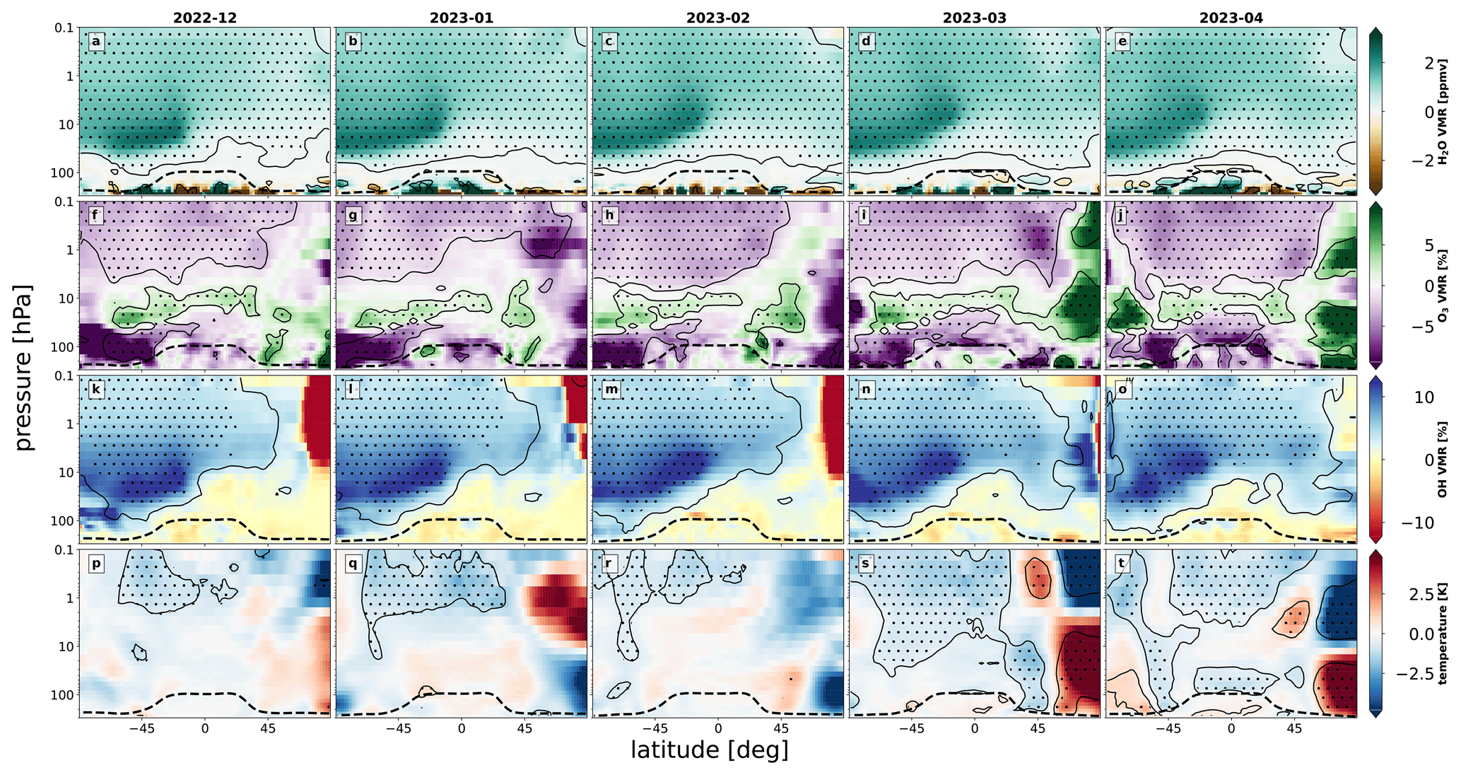
Figure 1 Monthly zonal-mean structure of the water vapour volume mixing ratio (VMR; first row of panels a–e; ppmv), ozone (second row of panels f–j; %), OH (third row of panels k–o; %), and temperature (fourth row of panels p–t; K) anomalies, respectively, for the extended boreal winter of 2022/2023. Anomalies are expressed as the difference between the SOCOLv4 simulations with and without the HT forcing. The 2σ statistical significance from the t test is indicated by the dots. The 1σ false detection rate (FDR) correction (see Sect. A2) is indicated by the black solid contour lines. The tropopause pressure level is indicated by the black dashed line.

As a consequence, the weakened winds allow more planetary waves (PWs) to propagate upward into the stratosphere (Charney and Drazin, 1961), where they break and dissipate and thereby further weaken the already disturbed stratospheric PV. The slowdown of the winds and the associated increase in polar temperature (see Fig. 2b) emerges in our simulations as early as February but is fully evident in March 2023. The stratospheric polar warming connected with the enhanced Brewer–Dobson circulation is directly coupled to the cooling aloft and the associated weaker meridional circulation. Furthermore, along with the temperature change, we detected (subsequently) increasing concentrations of ozone over the polar cap in March and April (see Figs. 1i–j or 13 in Fleming et al., 2024). The temperature structure across the upper atmosphere displayed in Fig. 2 resembles the transition from a more positive phase to a more negative phase of the Northern Annular Mode (NAM; see Sect. A3) in the stratosphere and lower mesosphere, respectively. Figure 2c illustrates how the HT forcing projects onto NAM (shading). Along with NAM we provide the eddy heat flux (EHF; green line) at 100 hPa as a proxy for upward propagation of planetary waves (e.g. Newman et al., 2001). The downward phase propagation of negative NAM anomalies illustrates the role of wave–mean flow interactions (Baldwin and Dunkerton, 2001), as also indicated by Eliassen–Palm flux diagnostics (see Fig. A7). Since the EHF response lags slightly behind NAM, the triggering mechanism appears to be similar to SSWs and how dynamically forced anomalies in the upper stratosphere and lower mesosphere may be communicated downward and thus control PWs (Hitchcock and Haynes, 2016).

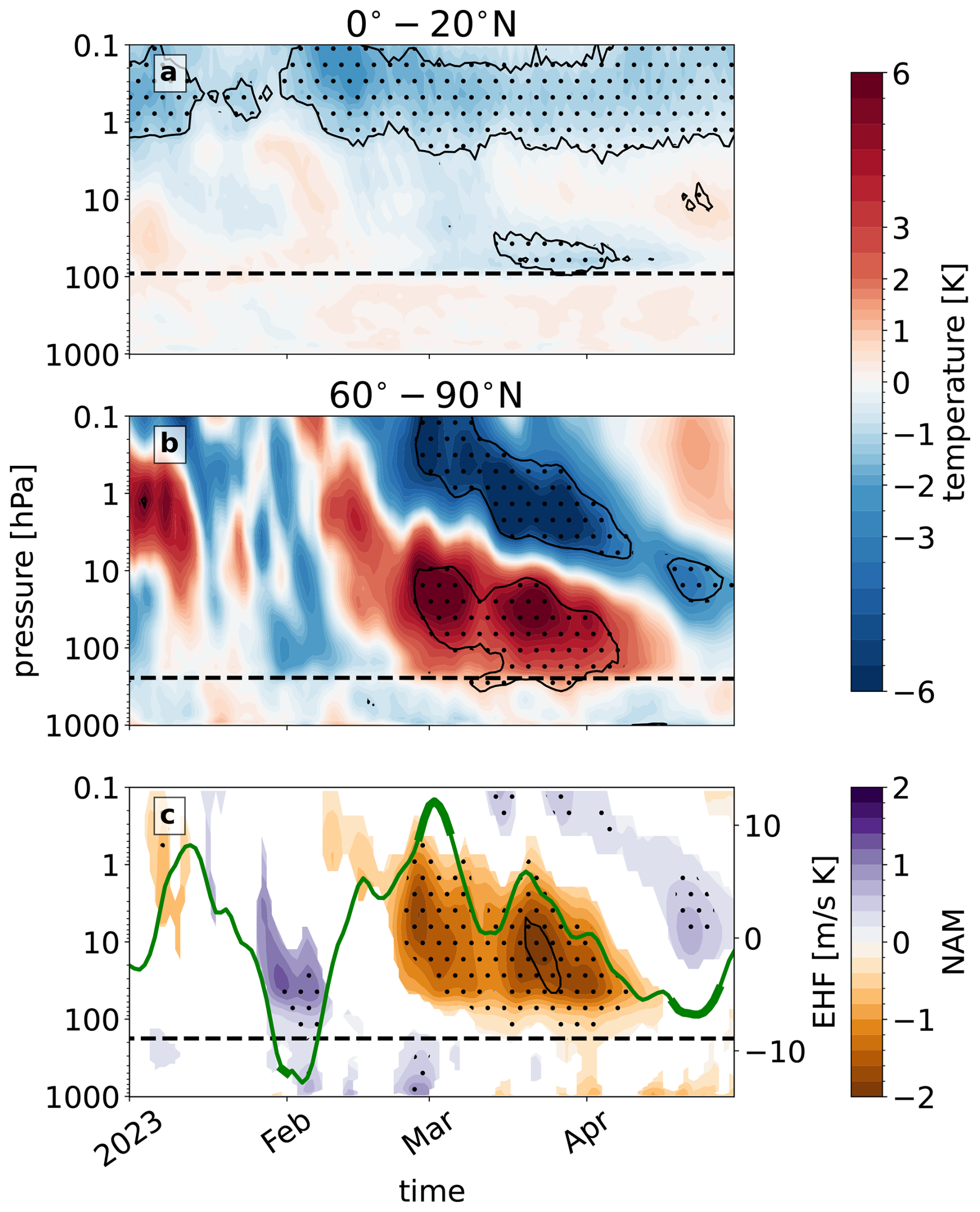
Figure 2 Weighted zonally averaged temperature averaged over 0–20° N (a) and 60–90° N (b) together with the Northern Annular Mode (NAM; shading in panel c) and eddy heat flux at 100 hPa averaged over 45–75° N (EHF in m s⁻¹ K; green line in c) daily anomalies for the months January to April in 2023. The anomalies are expressed as the differences between the SOCOLv4 simulations with and without HT forcing. The 2σ statistical significance from a t test is indicated by the dots. The 1σ FDR correction (see Sect. A2) is indicated by the black solid contour lines. To highlight the signal propagation, we mask out insignificant NAM values at 1σ.

Turning the focus to the lower levels, it becomes apparent that negative NAM anomalies emerge close to the surface (∼ 1000 hPa) in April and follow the significant negative NAM anomalies in the stratosphere in the preceding months. This time lag suggests that stratospheric anomalies are triggering some of the changes observed in the troposphere (Thompson et al., 2005). Geopotential height anomalies (see Fig. A8) again support a downward propagation of the signal from the stratosphere all the way to the surface. To explore these conditions further, we turn the focus to the analysis of the monthly sea level pressure (SLP; hPa) anomaly in April 2023, which is shown in Fig. 3. Here we identify a positive SLP anomaly at the poles and a negative SLP anomaly at the mid-latitudes. This pattern is characteristic of a weaker stratospheric PV and is associated with an equatorward shift of the tropospheric jet stream. The canonical temperature pattern with a pronounced cold anomaly in northern Europe (see Fig. 3b) clearly arises for this weak vortex event (Domeisen and Butler, 2020; Kolstad et al., 2022). Generally, the coupling is independent of the forcing mechanism causing these changes in PV and is present across all the timescales (Kidston et al., 2015).

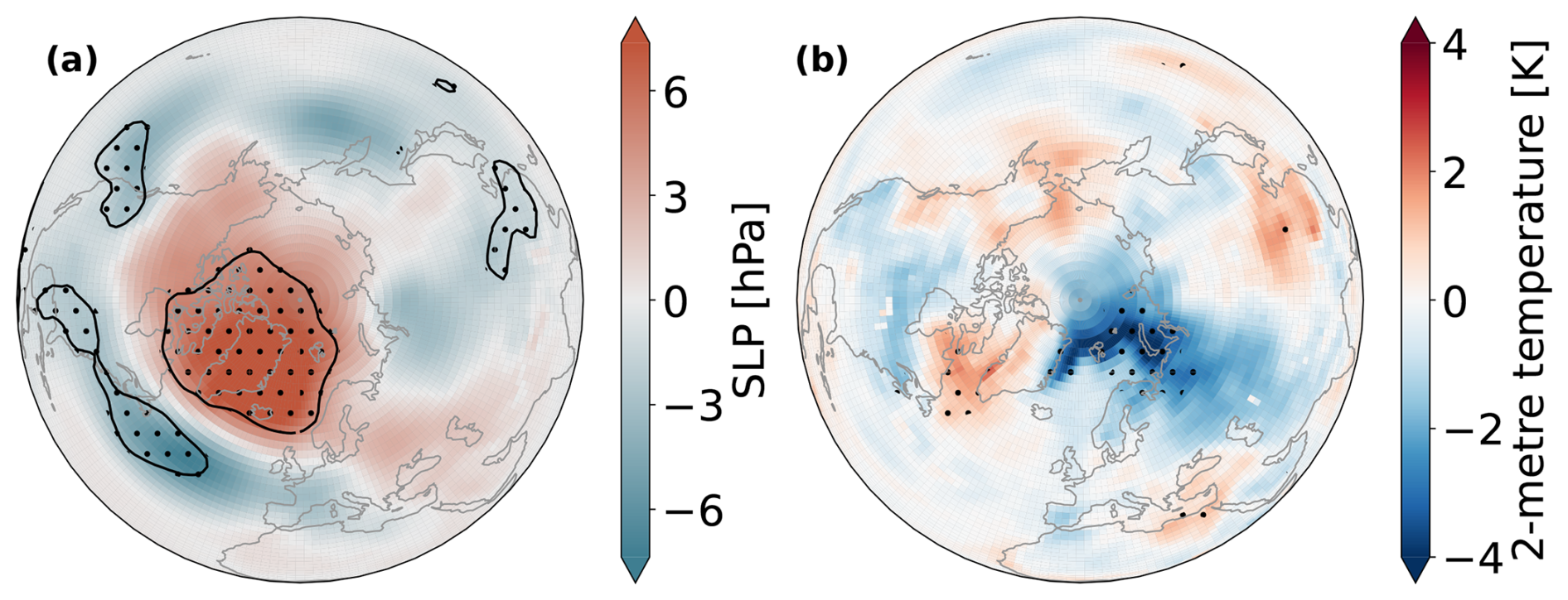
Figure 3 Monthly anomaly of sea level pressure (a; SLP; hPa) and surface air temperature (b; K) in April 2023. Anomalies are expressed as the differences between the SOCOLv4 simulation with and without the HT forcing. The 2σ statistical significance from the t test is indicated by the dots. The 1σ FDR correction (see Sect. A2) is indicated by the black solid contour lines.

3 Discussion and summary

The January 2022 Hunga Tonga–Hunga Ha'apai volcanic eruption significantly modified the radiative balance, photochemistry, and dynamics of the stratosphere and lower mesosphere, as has been extensively documented (Coy et al., 2022; Sellitto et al., 2022; Jenkins et al., 2023; Santee et al., 2023). Here we add to the discussion of HT effects by illustrating for the first time the dynamical stratosphere–troposphere–surface coupling in the NH following the eruption. We show in a series of ESM sensitivity simulations how the WV input propagated upward and poleward, thereby impacted the stratospheric PV, and contributed to the emergence of SSW in the boreal winter of 2022/2023 and subsequent surface SLP anomalies. Similarly, the HT eruption induced a marked warming anomaly in the Arctic region, with temperatures rising by up to 2 K near the North Pole in early 2022 (Bao et al., 2023).

Our results thereby illustrate how anomalies in OH, nitrogen species, and O₃, induced in the stratosphere and lower mesosphere due to excess WV after the HT eruption, influence upper-atmospheric dynamics via alteration of temperature gradients and thereby lead to the emergence of a negative NAM anomaly at upper levels during the winter–spring transition that manifests by April 2023 in SLP. We begin our attribution in the upper stratosphere and lower mesosphere, where increased OH concentrations induce a negative ozone anomaly. As a consequence, our set of sensitivity simulations illustrates a radiatively induced negative temperature response in equatorial latitudes up to 20° N, which leads to a reduced horizontal hemispheric temperature gradient. This alteration of the temperature gradient is associated with weaker winds via the thermal wind relation. As weaker winds emerge in the stratosphere (negative NAM anomaly), we find that the anomaly propagates downward with time, illustrating the role of wave–mean flow interactions, similarly to during SSWs. This mechanism provides a summary of a chain of processes which could have contributed to the observed SSW during the winter of 2022/2023. We note that the causal link in observations cannot be entirely established on the one hand due to internal stratospheric variability driving SSWs (Baldwin et al., 2021) and on the other hand the free-running ocean setup of our simulations. However, all other things being equal, our results clearly show that HT has provided favorable conditions for the emergence of late-winter NH SSWs in 2023.

Two major SSWs were detected during the extended winter of 2023/2024 (see Fig. A9). Our model-projected forcing during that winter was weaker due to a quicker WV dissipation from the stratosphere (see Fig. A4). Thus, we do not detect any significant dynamical responses. While Randel et al. (2024) observed strong (∼ −2 K) lower-mesospheric cooling after mid-2023, the mechanism suggested and simulated by SOCOLv4 above should be valid for the winter of 2024 and the following winters if the lower-mesospheric cooling is persistent and strong enough due to the excess WV. This mechanism establishes a novel pathway by which water-rich volcanic eruptions can indirectly impact the surface climate via downward propagation of the dynamical perturbation from the stratosphere and lower mesosphere. Thereby it adds to the manifestations of stratosphere–troposphere coupling on various timescales.

Future work should vet the proposed mechanism, ideally within multimodel intercomparison projects (Zhu et al., 2024), and explore whether the HT forcing also contributed to the disruption of the stratospheric PV during the following winters. Given the interhemispheric extent of cooling in the upper stratosphere and lower mesosphere, which could similarly affect the persistence of PV in the SH, future studies could explore the PV response in the SH and its coupling with the troposphere. Furthermore, the stratospheric response could be impacted by the phase of the Quasi‐Biennial Oscillation, as recently suggested by Jucker et al. (2024).

Appendix A: Methods

A1 SOCOLv4 simulations

We use a set of ensemble sensitivity simulations performed with the Earth system model SOCOLv4 (Sukhodolov et al., 2021), which comprises comprehensive stratospheric chemistry and sulfate aerosol microphysics, to assess the impacts of the HT eruption on stratospheric composition and dynamics. SOCOLv4 is used at a T63 horizontal resolution (1.9°×1.9°) and a vertical resolution of 47 vertical levels (up to ∼ 0.01 hPa), with the boundary conditions following the recommendations of the Coupled Model Intercomparison Project Phase 6 (CMIP6; Eyring et al., 2016). The Quasi‐Biennial Oscillation (QBO) is not self-generated with the employed vertical resolution, and therefore it is nudged in the model. Since the simulations expand into the future, instead of the actual QBO observational data, we used the same data but shifted back by 16 years, allowing us to keep a QBO phase during the eruption that is consistent with observations. The SOCOLv4 model is widely used for process analyses in stratospheric research and has contributed to the recent Chemistry-Climate Model Initiative (CCMI; Morgenstern et al., 2022; Friedel et al., 2023) and the Interactive Stratospheric Aerosol Model Intercomparison (ISA-MIP: Quaglia et al., 2023; Brodowsky et al., 2024).

Our set of simulations comprises an ensemble of transient simulations with and without HT forcing. We perform a 5-year spinup prior to the HT eruption, so that by the date of the event each ensemble member has a different ocean state contributing to the internal variability in the ensemble. In January 2022 we then branch out to two ensembles, one with and one without the HT forcing. Both ensembles comprise 10 ensemble members. Note that the WV freezing around the emission region (22–14° S, 182–186° E; 25–30 km within 15 January) was turned off for several days to avoid artifacts and mimic the estimated magnitude (∼ 150 Tg) of the WV forcing by Millán et al. (2022) and M2-SCREAM (see Fig. A1a; Wargan et al., 2023). Another way of avoiding freezing artifacts would be to broaden the emission region vertically. The M2-SCREAM WV anomaly is within the ensemble spread; however, this spread is quite wide, suggesting that the WV plume evolution could have been strongly modulated by the background dynamical conditions. In addition, the modelled WV anomaly shows a more pronounced seasonal cycle.

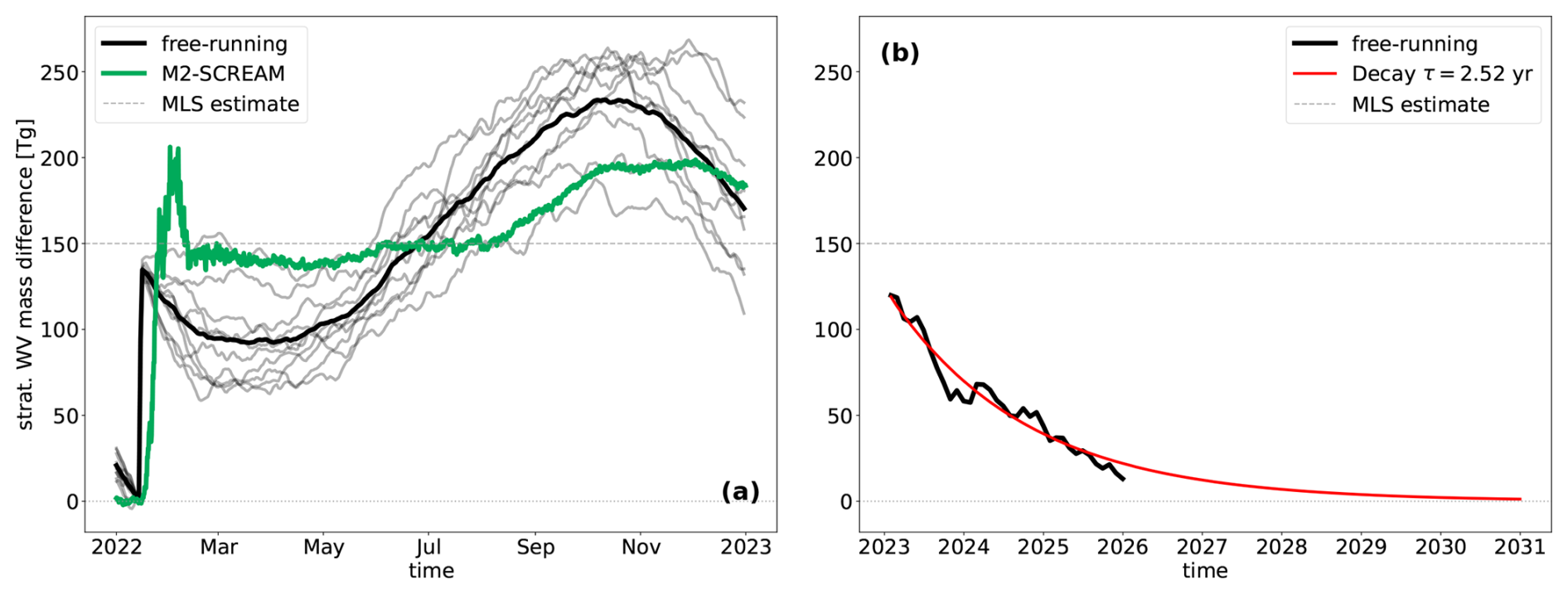
Figure A1 (a) Globally averaged daily anomaly of integrated stratospheric water vapour during January 2022 for the free-running (black line) SOCOLv4 simulations and M2-SCREAM (green line) with respect to 14 January 2022. (b) Monthly anomaly of integrated stratospheric water vapour for the free-running SOCOLv4 simulations (black line) for the period 2023–2025 and the corresponding fitted decay (red line) with an e-folding time τ of 2.52 years. The horizontal dotted line represents the magnitude after the HT eruption estimated by Millán et al. (2022).

According to the fitted decay, we project the stratospheric WV burden to represent an enhanced forcing over the next few years and only return to pre-HT background values by 2031. The excess stratospheric WV returns to the troposphere by sedimentation of PSCs within the SH PV and is transported to the higher latitudes of both hemispheres via the Brewer–Dobson circulation (BDC). The combination of these processes leads to an exponential decay of the WV burden with an estimated e-folding time of ∼ 2.5 years based on the fitted period of 2023–2025 (see Fig. A1b). Our decay estimate is in agreement with Fleming et al. (2024), who used a free-running 2D model, but it is about half of the estimate provided by Zhou et al. (2024), who estimated an e-folding timescale of 4 years using a chemical transport model with the perpetual ERA5 meteorology.

Furthermore, we use data from SWOOSH for the daily H₂O (Davis et al., 2016) and from GloSSAC for the monthly mean surface area density (SAD; NASA/LARC/SD/ASDC, 2023) to validate the SOCOLv4 anomalies (see Figs. A2 and A3). Note that we retrieve SAD fields using aerosol extinction coefficients on all four GloSSAC wavelengths according to the REMAP method (Jörimann, 2025). The SAD background in GloSSAC is a bit higher at higher latitudes compared to SOCOLv4 since for GloSSAC we used the 1999–2004 climatology representative of volcanically quiescent conditions, while for SOCOLv4 we used the difference between experiments with and without HT. The aerosol plume evolves in a similar spatiotemporal manner, i.e. towards the SH and lower pressure levels. The WV plume extends horizontally, firstly towards the SH PV and then across the Equator according to the climatology of the residual circulation. During the boreal winter of 2023, the WV anomaly is spread across all latitudes from the middle stratosphere upward in both SWOOSH and SOCOLv4. The reduction in water in SOCOLv4 starts to be apparent at the end of 2023, in contrast to SWOOSH, where the WV anomaly maintains its values. The globally averaged stratospheric and lower-mesospheric water vapour in Fig. A4 indicates a slight deficiency of SOCOLv4 as the anomalous water dissipates more quickly, as seen in the observations (e.g. the Microwave Limb Sounder – MLS) or the other models (see WACCM in Figs. 1, 2, and 3 in Randel et al., 2024). Note that our experiment protocol differs from WACCM and the other models (Zhu et al., 2024), which were either nudged to reanalysis or initialized from the observed sea surface temperatures.

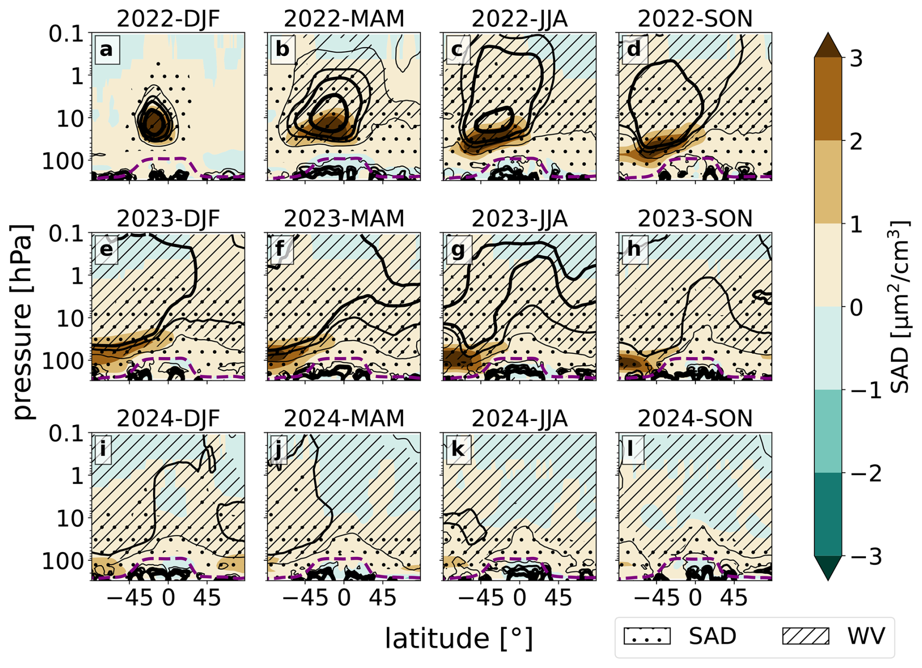
Figure A2 Seasonal zonal-mean structure of surface area density (SAD; shading; µm² cm⁻³) and water vapour (WV; solid contour lines: $\mathrm{0.1},\mathrm{0.5},\mathrm{1}$, and 3 ppmv) volume mixing ratios. Anomalies are expressed as differences between the SOCOLv4 simulations with and without the HT forcing. The 2σ statistical significance from the t test is indicated by the dots and hatching in the cases of SAD and WV, respectively. The tropopause pressure level is visualized by the purple dashed lines.

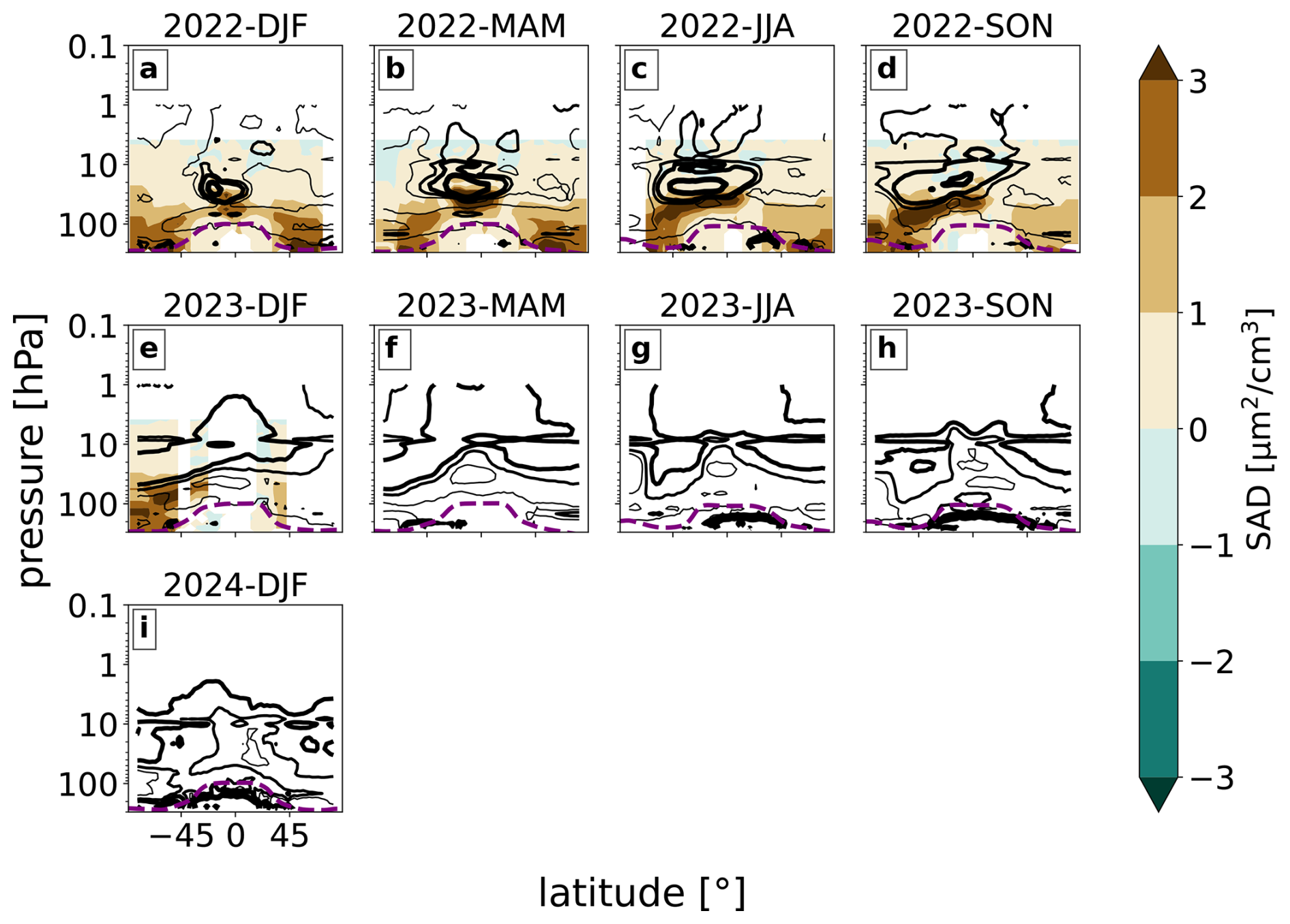
Figure A3 Seasonal zonal-mean structure of the SAD (shading; µm² cm⁻³) and WV (solid contour lines: 0.1, 0.5, 1, and 3 ppmv) volume mixing ratios. The SAD and WV anomalies in GloSSAC and SWOOSH are expressed as differences with respect to the climatology for the periods 1999–2004 and 1984–2023, respectively. The tropopause pressure level is visualized by the purple dashed line.

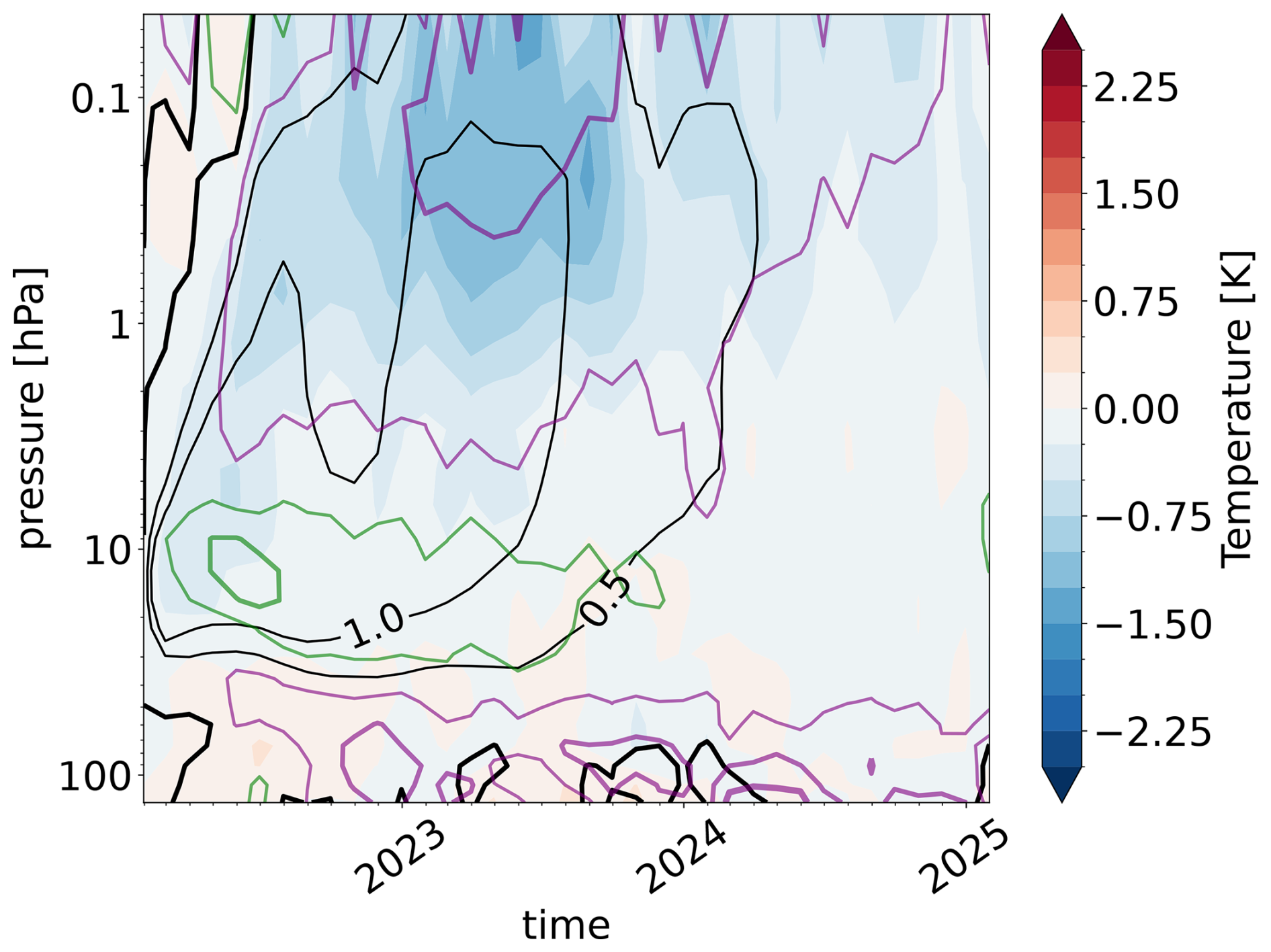
Figure A4 Monthly global-mean evolution of the temperature (shading; K), water vapour volume mixing ratio (black solid contour lines: $\mathrm{0},\mathrm{0.5},\mathrm{1}$, and 3 ppmv), and ozone volume mixing ratio (%; purple solid contour lines −5, −3, and −1; green solid contour lines 1,3, and 5) between 100 and 0.01 hPa. The anomalies are expressed as differences between the SOCOLv4 simulations with and without the HT forcing.

The overly strong tropical-to-midlatitude mixing and the overly fast tropical ascent are common peculiarities for chemistry-climate models (Dietmüller et al., 2018). As has already been reported (Sukhodolov et al., 2021), this could be addressed in future simulations with higher vertical resolution (Brodowsky et al., 2021). Nevertheless, during late 2022 and early 2023 the model is in good agreement with observations in terms of the WV and aerosol forcing.

A2 Calculation of anomalies

Throughout our analysis we evaluate significance fields using the minimum local p values from a Student's t test with global test statistics and the FDR methodology (Wilks, 2006) first described by Benjamini and Hochberg (1995) and later promoted by Wilks (2016) in the atmospheric sciences. All the illustrations in Sect. 2 show differences between simulations with and without HT forcing. For the significance regions we show, in addition to the dots indicating local p values <0.05, boundaries of p values <0.32 corrected for FDR.

A3 Calculation of the Northern Annular Mode

NAM was calculated at each pressure level as the first empirical orthogonal function (EOF) of the daily, latitude-weighted, and zonal-mean zonal wind poleward of the NH (Gerber et al., 2008). The NAM index was defined as the principal component time series associated with the first EOF and was standardized. Positive and negative NAM values correspond to strong and weak PV events, respectively, with different thresholds used for the SSW identification (Baldwin and Dunkerton, 2001; Gerber and Polvani, 2009; Jucker, 2016).

A4 Eliassen–Palm flux diagnostics

The response of resolved waves is investigated using the EPF diagnostics (Andrews and McIntyre, 1987). EPFs are computed and scaled following Jucker (2021). The EPF convergence serves as an indicator of wave dissipation, and the EPF divergence (EPFD) indicates sourcing.

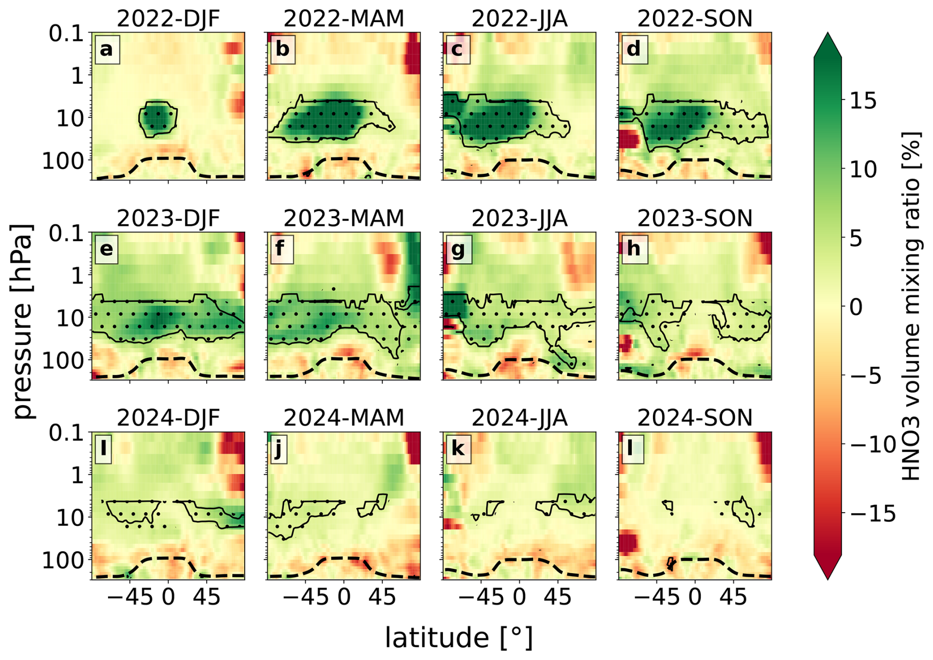
Figure A5 Seasonal zonal-mean structure of the HNO₃ volume mixing ratio (a–l; %). Anomalies are expressed as differences in the SOCOLv4 simulation with and without the HT forcing. The 2σ statistical significance from the t test is indicated by the dots. The 1σ FDR correction (see Sect. A2) is indicated by the black solid contour lines. The tropopause pressure level is visualized by the black dashed line.

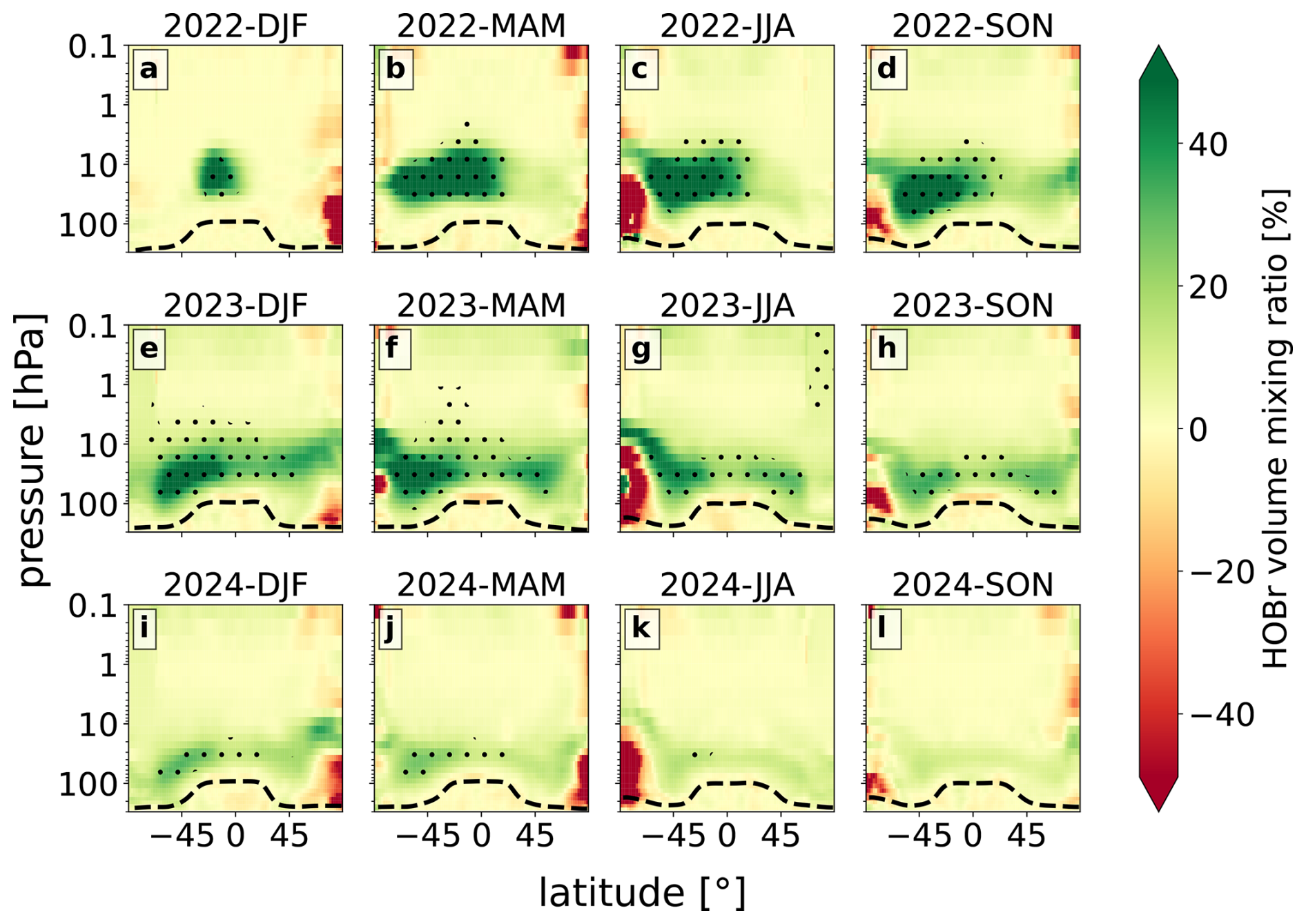
Figure A6 Seasonal zonal-mean structure of the HOBr volume mixing ratio (a–l; %). Anomalies are expressed as differences in the SOCOLv4 simulation with and without the HT forcing. The 2σ statistical significance from the t test is indicated by the dots. The 1σ FDR correction (see Sect. A2) is indicated by the black solid contour lines. The tropopause pressure level is visualized by the black dashed line.

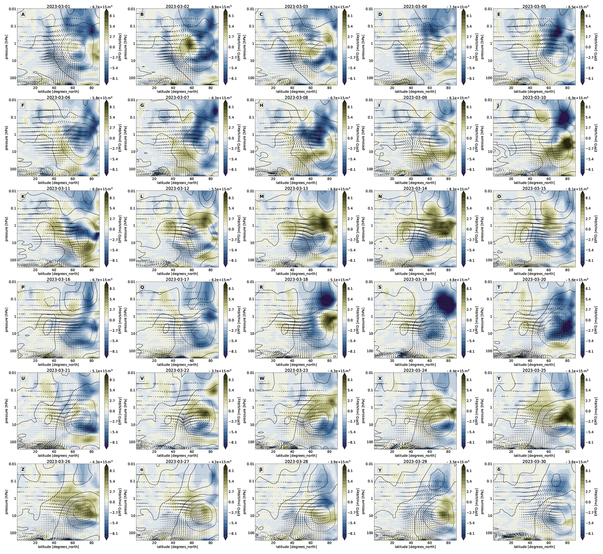
Figure A7 Daily anomalies of the EPF (arrows; m² s⁻² and hPa m s⁻²), its divergence (EPFD; shading; m s⁻¹ d⁻¹), and its zonal-mean zonal wind (solid (positive) and dashed (negative) contours; m s⁻¹) in March 2023.

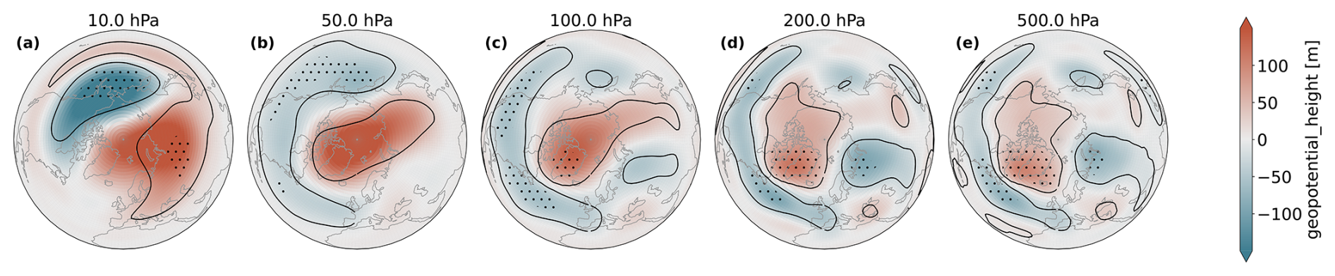
Figure A8 Monthly geopotential height anomalies (shading; m) at 10, 50, 100, 200, and 500 hPa in April 2023. The 2σ statistical significance from the t test is indicated by the dots. The 1σ FDR correction (see Sect. A2) is indicated by the black solid contour lines.

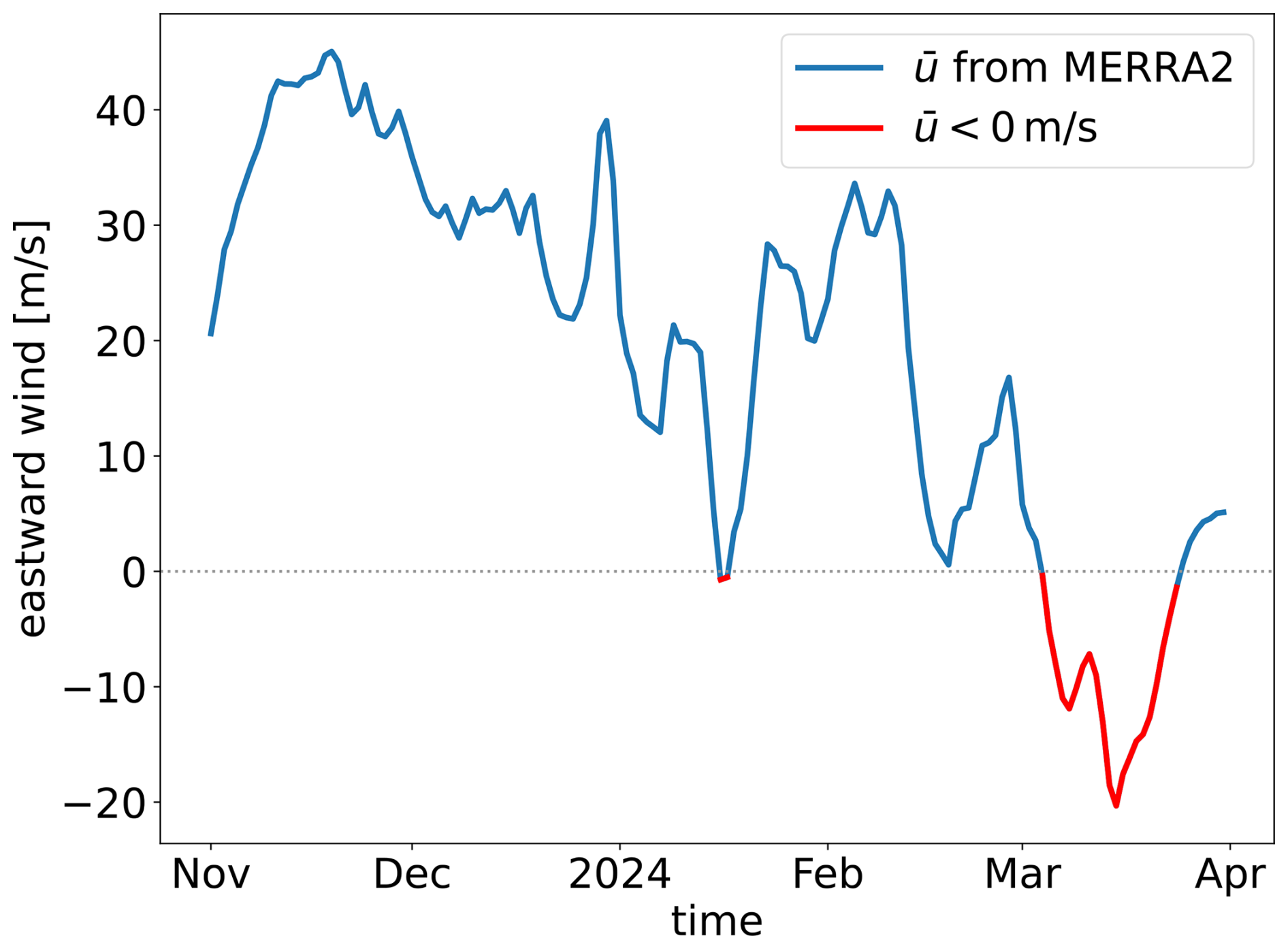
Figure A9 Daily zonal-mean zonal wind at 10 hPa and 60° N based on the MERRA2 dataset (Gelaro et al., 2017). It documents two major SSWs in the 2023/2024 winter.