The ZiCOS-M CO₂ sensor network: measurement performance and CO₂ variability across Zurich

As a component of the ICOS Cities project, a “mid-cost” NDIR (nondispersive infrared) CO₂ sensor network was deployed across the city of Zurich (Switzerland), known as ZiCOS-M. The network was operational between July 2022 and July 2024 and consisted of 26 monitoring sites, 21 of which were located in or around the city of Zurich, with 5 sites outside the urban area. Daily calibrations using two reference gas cylinders and corrections of the sensors' spectroscopic response to water vapour were performed to reach a high level of measurement accuracy. The hourly mean root mean squared error (RMSE) was 0.98 ppm (range of 0.46 and 1.5 ppm) and the mean bias ranged between −0.72 and 0.66 ppm when undergoing parallel measurements with a high-precision reference gas analyser for a period of 2 weeks or more. CO₂ concentrations (technically, dry-air mole fractions) were highly variable with site means in Zurich ranging from 434 to 460 ppm, and Zurich's mean urban CO₂ dome was 15.4 ppm above the regional background. Some of the highest CO₂ levels were found at two sites exposed to strong plant respiration in a very confined nocturnal boundary layer. High-CO₂ episodes were detected outside Zurich's urban area, demonstrating that processes acting on a variety of scales drove CO₂ levels. The ZiCOS-M network offered significant insights at a cost an order of magnitude lower compared to reference instruments, and the observations generated by ZiCOS-M will be used in additional ICOS Cities activities to conduct CO₂ emission inventory validation with inversion modelling systems.

1 Introduction

1.1 Background

Urban areas are very significant sources of atmospheric pollutants and greenhouse gases (GHGs), including carbon dioxide (CO₂). In 2020, it was estimated that urban areas were responsible for approximately 70 % of global CO₂ emissions (Lwasa et al., 2022). Increased population densities and intensive energy consumption can result in CO₂ urban domes, where CO₂ is enhanced by a few parts per million (ppm) to tens of ppm in and around the urban extent (Xueref-Remy et al., 2023). Reducing CO₂ emissions and the decoupling of carbon emissions from economic growth are priorities for most national and subnational governments in order to avoid some of the worst negative consequences of anthropogenic climate change (IPCC, 2023). The importance of CO₂ emissions from urban areas has driven top-down analysis methods, where observations of CO₂ are combined with atmospheric inversion modelling systems to validate bottom-up emission inventory-based estimates. These two approaches (top-down and bottom-up) are complementary, and their reconciliation is expected to yield the most reliable emission estimates to allow for potential management.

The monitoring of CO₂ in urban areas has been a lesser priority when compared to the monitoring of traditional air pollutants because of the lack of legal standards for CO₂. Therefore, high-quality CO₂ time series are generally confined to isolated or remote locations where immediate emission sources are absent. These sites are suitable for capturing long-term and large-scale processes, but they are unable to resolve the dynamics of CO₂ sources and sinks within urban areas (Hernández-Paniagua et al., 2015). In addition, the technology used for high-accuracy monitoring of CO₂ measurement remains expensive (Mao et al., 2012; Martin et al., 2017), and, therefore, the deployment of several CO₂ analysers in a city is usually considered cost-prohibitive. An alternative approach is to deploy lower-cost CO₂ sensors, and several research groups have deployed monitoring networks in this context (Maag et al., 2018). Although such sensors have lower measurement performance, their poorer accuracy can be offset by being deployed in larger numbers, and thus, they offer the possibility of resolving spatial and temporal patterns at a smaller scale (Peltier et al., 2021). Therefore, the utility of lower-cost sensors can still be high (Bart et al., 2014; Casey and Hannigan, 2018).

Prominent urban CO₂ monitoring networks include the Berkeley Environmental Air-quality and CO₂ Network (BEACO₂N) located across the San Francisco Bay area (Shusterman et al., 2016; Turner et al., 2016; Kim et al., 2018; Delaria et al., 2021), the Indianapolis (INFLUX) Urban Test Bed (Turnbull et al., 2015; Davis et al., 2017), the Los Angeles Megacity Carbon Project (Verhulst et al., 2017), the Northeast Corridor tower network (Karion et al., 2020), networks in Paris (Arzoumanian et al., 2019; Lian et al., 2024), and the Carbosense network across Switzerland (Müller et al., 2020). The nomenclature regarding the cost points for these networks is inconsistent because the definition of what a lower-cost sensor is varies among operators. Here, we discuss a CO₂ sensor network that has been defined as “mid-cost” and is in a price range that is comparable to the BEACO₂N and Paris networks. The Carbosense network, in contrast, used sensors at a significantly lower price point and, therefore, would be defined as a low-cost CO₂ sensor network.

1.2 Switzerland and Zurich

Switzerland is a small country located in western Europe with a population of approximately 9 million. It is highly developed, with GDP per capita among the highest in the world (International Monetary Fund, 2023). Switzerland has been successful at decreasing its production-based CO₂ emissions, especially since 2010 (Ritchie et al., 2020; Federal Office for the Environment (FOEN), 2023). Consumption-based per capita CO₂ emissions have not decreased in the same way and remain high, reflecting the wealth of the country's residents.

Zurich is Switzerland's largest city and has a population of 430 000 inhabitants in the city proper and another 1 million in the surrounding agglomerations (Stadt Zürich, 2023a). Zurich is located on the Swiss plateau at about 410 m above sea level in an area of complex terrain. Zurich's city centre is situated around Lake Zurich's main northern outflow – the Limmat River – flowing in a north-west direction, which has formed the Limmat Valley, where much of the urban area is located. The Limmat Valley is bound to the west by the Albis range and to the east by the discontinuous Pfannenstiel–Altberg hill chain. Zurich's urban area extends beyond the Limmat Valley in all directions, but notably, districts 11 and 12 are located north of the eastern hill range and form a continuous urban area over a saddle between Zürichberg and Käferberg. These topographic features of the urban area are relevant to pollutant transport and dispersion processes (Berchet et al., 2017).

The city of Zurich's local government has legal obligations to reach net zero by 2040 regarding direct CO₂ emissions and has targets for the reduction in per capita emissions (Stadt Zürich, 2023b). These net-zero laws were a result of a Canton of Zurich referendum in September 2022. The latest emission inventory compiled for 2022 indicates that half of the city's CO₂ emissions (51 %) are sourced from stationary combustion, mostly residential and commercial heating emissions with a small contribution from waste incineration (Stadt Zürich, 2024). Public power generation and road transportation are the two other large emission sources (32 % and 12 %, respectively), and all other sources make up the outstanding 5 %.

1.3 ICOS Cities

ICOS Cities (https://www.icos-cp.eu/projects/icos-cities, last access: 24 February 2025) is a European Horizon 2020 project that acts as a pilot to test and evaluate different CO₂ measurement approaches that provide value for the scientific, policy, and citizen communities within urban areas. Three European cities ranging from large to small – Paris (France), Munich (Germany), and Zurich (Switzerland) – are included in the pilot project, and all three cities have CO₂ sensor networks that form one component of the urban observatories that have been or are deployed in the cities. By design, the three different sensor networks in the three cities differ in their monitoring focus, hardware, and software but not in their primary objectives. In the Zurich case, the ZiCOS-M network greatly benefited from the experiences gained from the earlier Swiss-wide Carbosense CO₂ network (Klose, 2017; Empa, 2019; Müller et al., 2020), but the Carbosense and ICOS Cities activities were separate.

The ZiCOS-M network was designed to supply observations for atmospheric inversion modelling systems in order to allow for comparisons between top-down estimates of CO₂ emissions (natural and anthropogenic) and bottom-up estimates. However, once the sensor network was deployed, it was clear that the network was providing observations at a sufficiently high data quality to be of use in observational analyses of CO₂ across the region of Zurich and its urban area.

1.4 Objectives

This work has two overarching objectives. The first is to describe the ZiCOS-M CO₂ sensor network's design, deployment, and data processing strategies and to document what measurement performance was achieved with the sensors. The second is to present the spatial and temporal patterns of CO₂ across the network's monitoring domain. The first objective will satisfy two communities: the inversion modelling groups that use the observations generated by the sensor network to evaluate and verify the city's emission inventory and those who are operating or designing environmental gas sensing networks because many of the data processing approaches are generic and are portable to other networks in other areas and/or networks that target other quantities, such as other greenhouse gases or air pollutants.

The CO₂ sensor network deployed across the city of Zurich for the ICOS Cities project contained two sensor tiers – so-called low-cost and mid-cost. Here, only the mid-cost sensors' activities and results will be discussed, while the low-cost sensor network (called ZiCOS-L) will be discussed in a future companion paper because the differing data quality gives rise to challenges when making direct comparisons across the different sensor types due to their different measurement performances.

At the time of writing, the ZiCOS-M network is still in operation, but imminently, the network will be reconfigured, whereby half of the monitoring sites will be decommissioned. Therefore, we refer to the ZiCOS-M's operations, sites, and data set in the past tense, except for with respect to the more distant background sites that are run by other monitoring activities because these sites can be considered permanent features.

2 Methods

2.1 Sensors

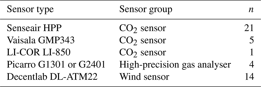
The ZiCOS-M network used three different models of NDIR (nondispersive infrared) CO₂ sensors from three different manufacturers. Most of the sensors (21) were an integration based on the Senseair HPP (high-performance platform) (Senseair, 2016, 2018) sensor (Table 1). The Senseair HPP sensor is a prototype sensor and is no longer in production. These sensors have seen use in similar past ambient monitoring activities in Switzerland (Müller et al., 2020), and related sensors have been characterised elsewhere (Kunz et al., 2018; Arzoumanian et al., 2019; Lian et al., 2024). In addition to the Senseair HPPs, five Vaisala GMP343 (Vaisala, 2013) sensor units were also used, and finally, one LI-COR LI-850 sensor (LI-COR Environmental, 2025) was operated in the network. The cost of the sensor units themselves was between CHF/EUR/USD 3000 and 5000, but after integration into a measurement system, the price point was approximately CHF/EUR/USD 5000–10 000. The counts of sensors in Table 1 do not include the replacement of the actual CO₂ sensors themselves within the sensor packages (which were referred to as sensing elements). Additionally, more sensors were operated than the number of monitoring sites because some sensors failed and were replaced during the monitoring period.

Table 1 The number (n) of different sensors or monitors used in the ZiCOS-M sensor network.

All three sensor models were integrated into a very similar monitoring package by Decentlab GmbH (Decentlab GmbH, 2022), a commercial project partner. Figure 1 shows the main components and configuration of the measurement system. The sensor package included three-way valves for the switching between ambient sampling and two gas cylinders with demand-flow regulators, filters, a sample pump, boards for data acquisition and transmission, temperature and relative humidity sensors installed in the sample gas stream, and for some integrations ambient air pressure sensors. Table A1 contains the make and models of the principal parts or components of the sensor packages. All hardware, except for the gas cylinders and demand-flow regulators, was contained in a weatherproof housing (Figs. 1 and A1). In the case of the Vaisala GMP343 and LI-COR LI-850 sensors, the ancillary sensors in the gas stream and the ambient pressure sensors were connected to the sensor and onboard compensations for sample temperature, humidity, and ambient pressure were enabled. Originally, it was planned that a consistent data processing approach could be used for the three sensor types, but due to their differing measurement performance (especially concerning water vapour), different logic was required. Full details of these processes are available in Sect. 2.3.

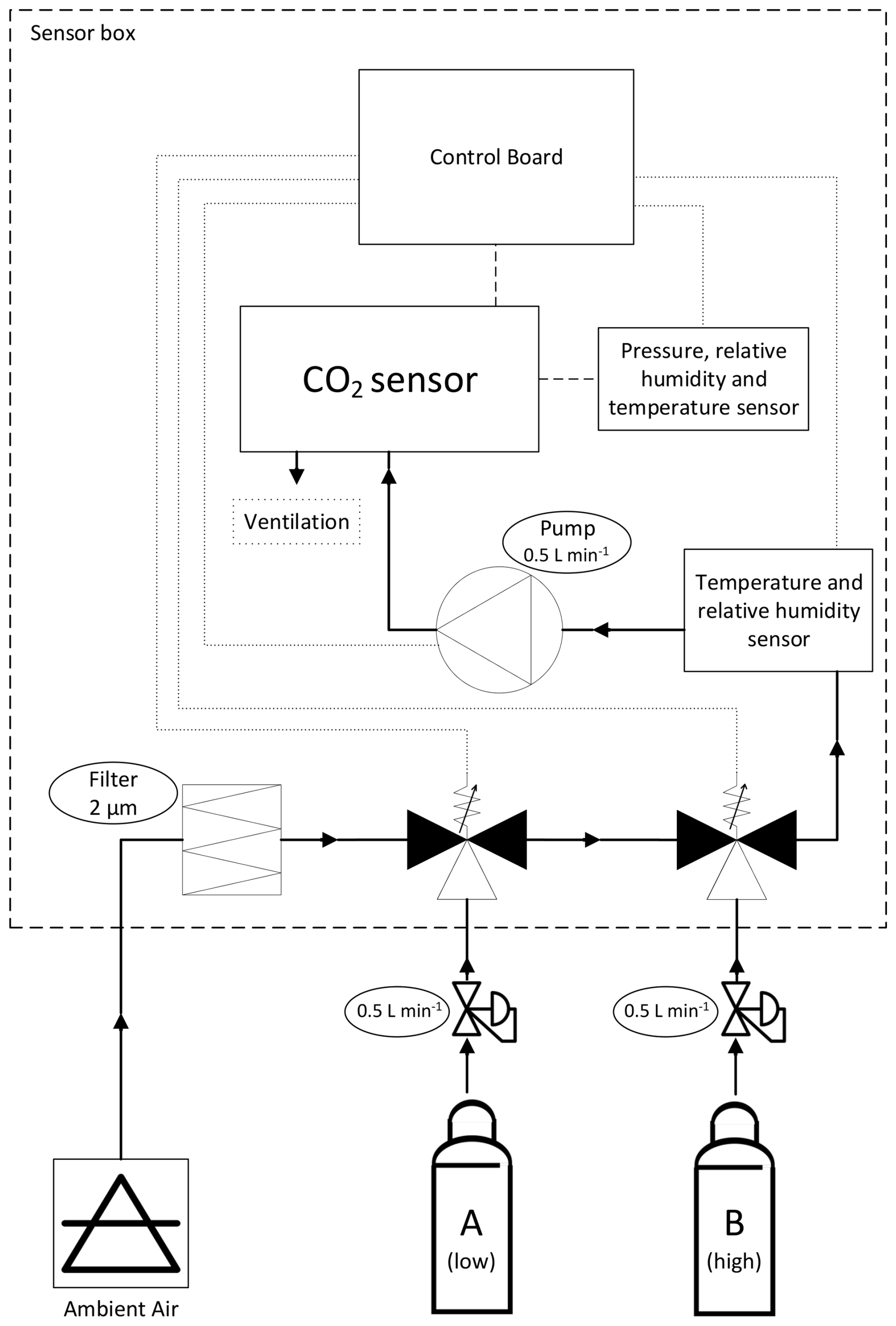
Figure 1 Schematic of the sensor measurement system showing the major components of the system and their configuration. Table A1 contains the make and models of the principal parts or components.

In addition to the CO₂ sensors, 14 sonic wind sensors (Decentlab DL-ATM22) were installed at rooftop sites to provide auxiliary information on airflow and temperatures in the city (Table 1). The sensors' data were transmitted via Swisscom's LoRaWAN network which is a wide-area network (WAN) designed for low-power applications and small data volumes (LoRa® Aliance, 2015). The four high-precision gas analysers included in the network's data set were cavity ring-down spectrometers of different generations manufactured by Picarro (Rella, 2010; Rella et al., 2013; Zellweger et al., 2016) that were operated by following routine calibration and data quality control processes.

2.2 CO₂ monitoring sites

The ZiCOS-M sensor network was composed of a total of 26 monitoring sites, with 21 sites in or around the immediate area of the city of Zurich and 5 sites in more distant locations. Three of these more distant sites were included in the data set as they provide critical information on CO₂ levels surrounding the city (Fig. 2; Table 2), while the other two sites provided CO₂ observations from other locations that could be contrasted with CO₂ measurements across the Zurich region.

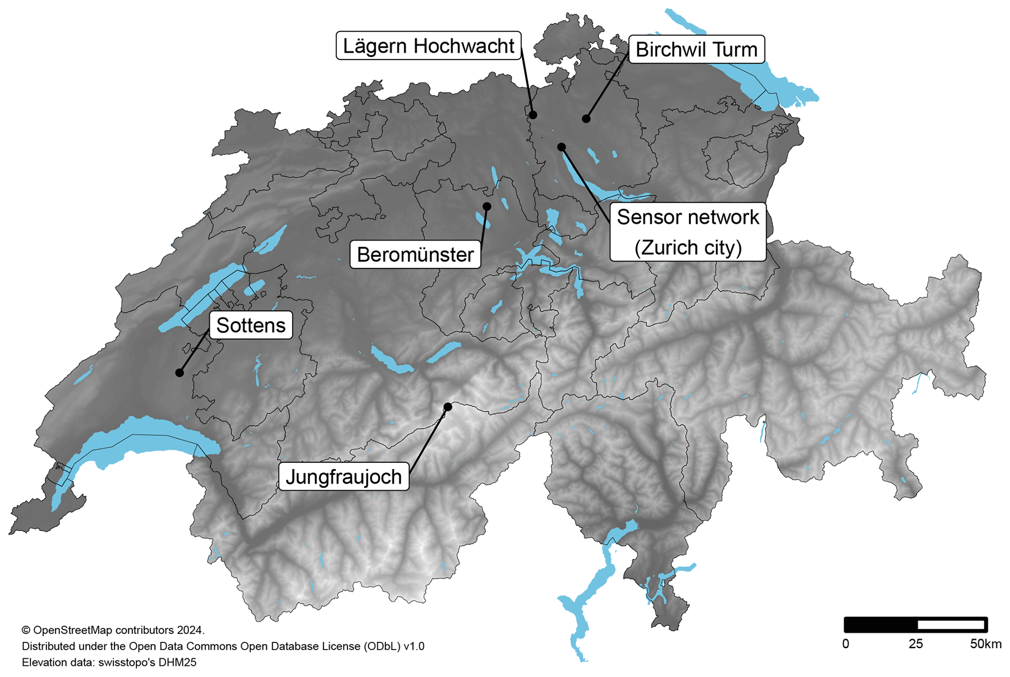
Figure 2 Location of the ZiCOS-M sensor network and the more distant locations where CO₂ observations were available and used as part of the study's data set in Switzerland. The internal lines indicate Switzerland's cantonal boundaries, and substantial waterbodies are also shown.

Table 2 Basic monitoring site information for the ZiCOS-M sensor network. The elevation represents the elevation above sea level of the monitoring site and the measurement height is the height above ground level. The five more distant and background sites outside Zurich are at the bottom of the table.

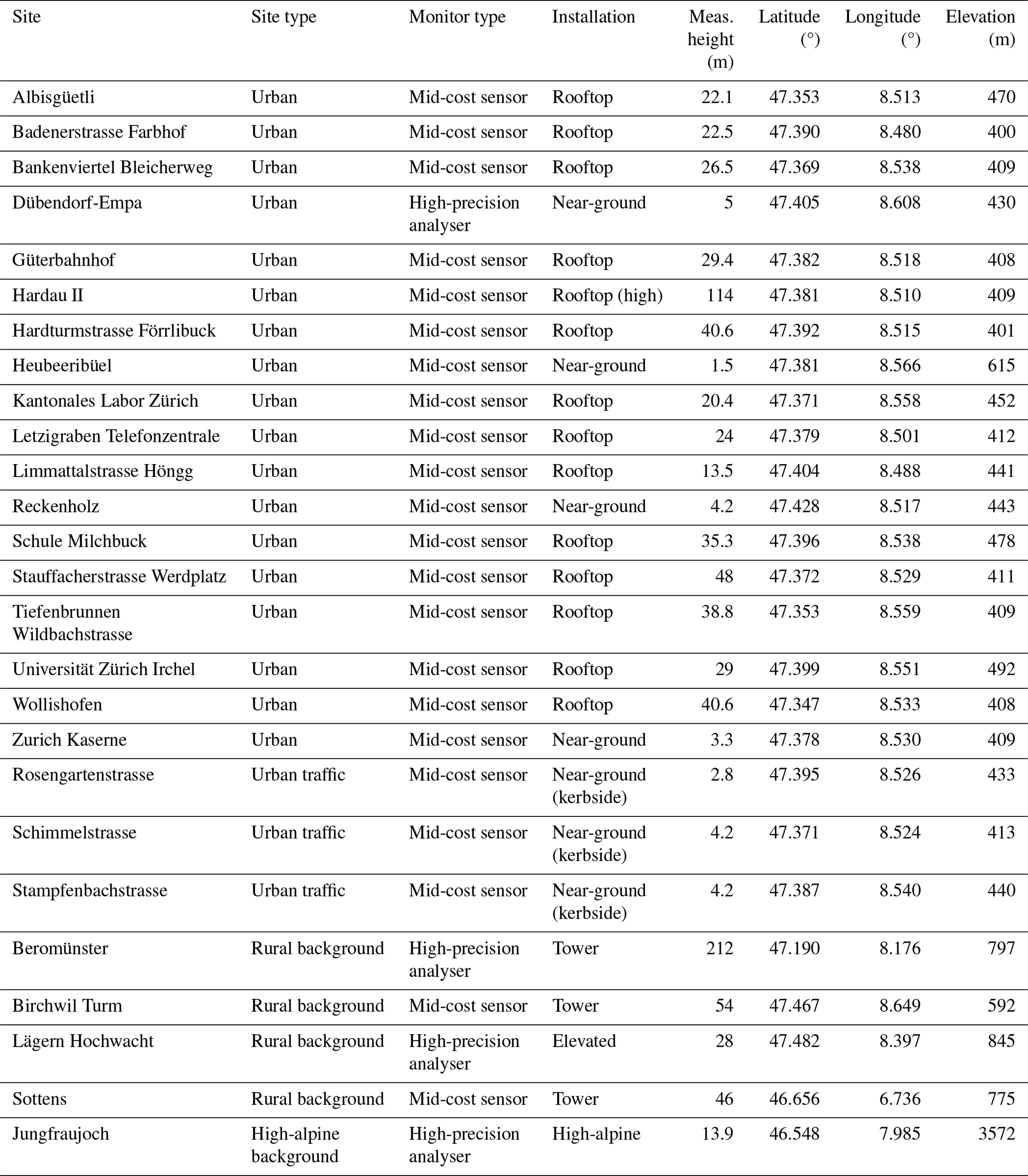
The network's testing site, Dübendorf-Empa, is also an air quality morning site that is part of the National Air Pollution Monitoring Network (NABEL) (Empa, 2024). Dübendorf-Empa was used for intercomparison exercises and model training using the reference CO₂ time series provided at this site. The intercomparisons conducted at Dübendorf-Empa allowed for the CO₂ sensors to be run in parallel with a high-precision gas analyser in ambient conditions for at least 2 weeks for a representative and robust testing procedure. Therefore, the measurement performance presented in Sect. 3.1 is highly representative of what was achieved during operational monitoring. Three of the four more distant sites were equipped with high-precision gas analysers, while the fourth site, Sottens (160 km to the south-west of the city of Zurich), had a sensor that was operated identically to those sensors in the city of Zurich. The predominant wind directions across the Zurich region are west-south-west and east-north-east, reflecting the orientation of the Swiss plateau. The three background monitoring sites surrounding the city of Zurich (Fig. 2) were positioned in locations that, depending on the wind behaviour, were down- or upwind of the city.

The Beromünster background monitoring site is located south-west of the city of Zurich (Fig. 2). It is a tall tower where the sampling system cycles between five different measurement heights. For the data set presented here, only observations from the highest sampling point at 212 m were used. Lägern Hochwacht is north-west of the city of Zurich and is located on the forested Lägern Hill that is orientated in an east–west direction. Lägern Hochwacht is on the hill's ridge or crest. The sampling height is 32 m above ground level (a.g.l.) which is above the forest's canopy height. For additional details about these two monitoring sites, see Oney et al. (2015). Birchwil Turm (a telecommunications tower) is another background site, located 12.8 km from Zurich's city centre in a north-east direction next to an electrical substation in the Zürcher Unterland (Table 2; Fig. 3). Birchwil Turm is approximately halfway between the city of Zurich and Winterthur, the Canton of Zurich's second largest city. Jungfraujoch in the Bernese Alps, 102 km from Zurich at an altitude of 3572 m, was used as the study's European or hemispheric background site (Fig. 2). Jungfraujoch is an observatory that includes NABEL and ICOS activities. The CO₂ time series from this location serves as a reference to represent background European CO₂ with an absence of any immediate significant emission sources (Pieber et al., 2022).

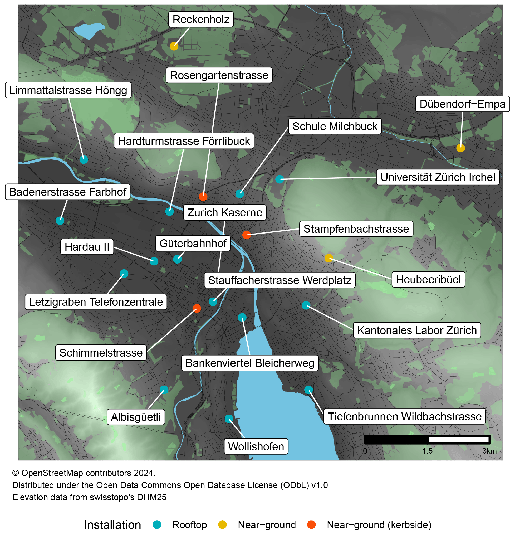
Figure 3 The ZiCOS-M CO₂ sensor sites (additional details can be found in Table 2) in and around the vicinity of the city of Zurich. Vegetated areas, terrain, and substantial waterbodies are also shown.

The monitoring sites within and around the city of Zurich were classified further by their installation or siting types. The majority of sensors (14 of the 22 sensor sites) were deployed with inlets sampling at rooftop level (Table 2; Figs. 3 and A1). The sensors were generally installed in maintenance rooms reserved for mobile phone infrastructure, and for most installations, these rooms were temperature-controlled. Rooftop installations were focused on to represent CO₂ emission sources in the city without being primarily forced by immediate emission sources as would occur with sampling points at ground level in street canyon environments. The rooftop sites offer spatial representativeness across the city at a resolution that was optimised to the mesoscale model systems' spatial resolution. The sites were carefully selected out of a large number of potential locations by requiring minimal impact from nearby ventilation or heating stacks that were present on many roofs.

Hardau II is a central monitoring site of the network, which features not only a mid-cost sensor but also an eddy covariance system to directly measure the CO₂ fluxes in a central part of the city. Measurements are conducted at 114 $\mathrm{m}\mathrm{a}.\mathrm{g}.\mathrm{l}.$ on a 95.3 m tall building, which is much higher than other rooftop sites. Several extra monitoring activities were conducted at this site during an intensive campaign between September 2022 and March 2023 within the ICOS Cities project. Details on the other monitoring activities at Hardau II are available in Stagakis et al. (2023).

2.3 Data

The principal steps of the extensive data processing for the ZiCOS-M network are outlined and explained below. The data processing logic was dependent on the sensor type (Sect. 2.1) because of the sensors' variable performances relating to what onboard correction algorithms were activated. A schematic of data processing steps is shown in Fig. A2, and the main equations are presented in the Appendix. The final set of observations was classified as Level-2A following the processing levels proposed by Schneider et al. (2019).

At a high level, the data processing steps can be grouped into three operations: (i) the collection and formatting of data from different sources to conform to a formal data model and framework for convenient access and interaction; (ii) the application of various adjustment strategies to improve the measurement quality without moving to outright model predictions (Schneider et al., 2019); and (iii) the handling and integration of metadata units such as when and where sensors were located, calibration gas information, and which observations have been invalidated and why. All data processing was conducted with the R programming language (R Core Team, 2023). The database technology used was PostgreSQL (PostgreSQL Global Development Group, 2024), and the formal time series relational data model was an extended smonitor data model previously developed for air quality applications that overlaps with greenhouse gas monitoring almost completely (Grange et al., 2017; Grange, 2018, 2019a, b).

2.3.1 Transmission and storage

All sensor data were transmitted through the LoRaWAN network to Decentlab's cloud storage infrastructure (Decentlab GmbH, 2022), where the data packets were decoded and made accessible via a simple application programming interface (API) (Grange, 2024b). Depending on the sensor type, diagnostic variables along with raw measurement values (the IR signal in the specific case of NDIR sensors); ancillary data such as temperature, relative humidity, and pressure from other sensors integrated into the sensor product; and onboard calculated CO₂ concentration were transmitted and stored. In the smonitor nomenclature, the CO₂ calculated by onboard algorithms (that are generally proprietary) and coefficients determined by factory calibration was called reported CO₂. The sensors reported observations approximately every 60 s; however, because of limitations of the LoRaWAN protocol, usually 57–58 measurements were successfully transferred and stored per hour.

Several other data sources were accessed in an automated or semi-automated fashion. These data sources include observations from a CO₂ analyser installed at the Dübendorf-Empa NABEL monitoring site (Fig. 3), which was the facility used for field testing and parallel measurements; observations for two additional high-precision CO₂ analysers in Switzerland but outside the city of Zurich (Lägern Hochwacht and Beromünster; Fig. 2); observations for three NABEL monitoring sites that hosted meteorological instrumentation; two MeteoSwiss data sources – the VQEA33 data product that contains MeteoSwiss's “core” sites or stations that host a full suite of meteorological sensors (five sites in and around Zurich were available) and observations sourced from the IDAweb portal (MeteoSwiss, 2009) for five additional meteorological sites in and around the city of Zurich; and finally Jungfraujoch's high-alpine (at 3572 m altitude; Fig. 2) validated and near-real-time CO₂ observations from the ICOS Carbon Portal (Emmenegger et al., 2023, 2024). All of these data sources were integrated into the common data model and stored for uniform access and interaction.

2.3.2 Water dilution effect correction and dry-air mole fractions

Atmospheric CO₂ is usually reported as the dry-air mole fraction (in units of µmol mol⁻¹ or parts per million, ppm) because this quantity is preserved, not only during atmospheric transport, but also under processes changing the moisture content of the air (Tans and Thoning, 2020). Here, we often use the more generic term “concentration” interchangeably, but in all cases beyond reported CO₂, the more accurate definition of the dry-air mole fraction is correct.

All NDIR CO₂ sensors used in the network reported CO₂ in moist air. To convert this to dry-air mole fractions, an estimate of the water vapour in the gas sample was required, which was obtained from the ancillary temperature and relative humidity sensors installed in the gas stream and the ambient pressure sensors installed within the sensors' waterproof box. The vapour pressure of water was calculated from the relative humidity and the saturation vapour pressure according to the August–Roche–Magnus equation (Alduchov and Eskridge, 1996; Lawrence, 2005). This conversion to dry-air mole fractions is referred to as water dilution correction in the following text.

The Senseair HPP sensors also required their reported CO₂ to be explicitly normalised to standard atmospheric pressure (1013.25 hPa) before the dilution correction. This was necessary because a clear CO₂ dependence on ambient pressure was observed during testing, which indicated that the integrated pressure sensor was not properly used for onboard pressure normalisation. This extra transformation was not required for the two other sensor types as they did not show a dependence on air pressure during the same tests.

2.3.3 Reference gas cylinder calibrations

The sensors were integrated with three inlets, an inlet for ambient air sampling and two inlets for the connection of two reference gas cylinders containing known CO₂ traceable to the WMO CO₂ X2019 calibration scale (Hall et al., 2021). Across the network, the sensors were deployed with 5 or 10 L “high” and “low” reference gas cylinders (≈ 400 and ≈ 600 ppm, respectively; Fig. 1). The inlets were switched from ambient to low and high inlets (in that order) every 25 h for 10 min. The first preceding and 4 subsequent minutes before and after the gas tests were handled as a non-ambient sample to ensure the sample system was flushed of cylinder-sourced gases and did not contaminate the ambient samples.

For each gas test, the period was isolated, the first and final 3 min were discarded, and the median was taken to represent the sensor's CO₂ for the cylinder test. This trimming and summary logic robustly captured the CO₂ concentration in the gas stream from the cylinder after the sensor had reached stability and the gas stream's flow, pressure, and humidity had the opportunity to equilibrate during the test period. Because the calibration gases were nearly dry, a gas sample humidity criterion of less than 10 % relative humidity was applied to determine whether the test was valid. A moist sample indicated a leak or an empty cylinder. All test summaries were stored for later use.

The high and low test summaries were used to compute a slope and offset with simple linear regression – albeit (usually) with only two points. The final calibrated dry-air mole fraction was then computed from the reported dilution-corrected dry-air mole fraction (Fig. A2).

Infrequently, a gas test summary was correctly calculated, but the result was a clear outlier. This was usually driven by poor data capture or bad valve articulation during the gas test. Therefore, the gas test summaries were passed through an interquartile range filter to remove these outliers. The 3 d rolling means of the slope and offset coefficients were calculated to slightly smooth the coefficients and to avoid a relatively large change in a coefficient occurring when traversing the midnight boundary during the movement from one calendar day to the next (Fig. A3). If a daily test was missing due to operational issues, the application of a last observation carried forward process was applied to the coefficients.

All sensors were able to be successfully corrected for their relatively constant change in baseline and sensitivity over the monitoring period with the daily reference gas tests (an example is shown in Fig. A3). The remaining variability may be partly explained by spectroscopic effects driven by various changes in environmental conditions, such as temperature and pressure. When there is access to two-cylinder gas tests for such an adjustment, other strategies are also possible, for example, using the low gas for an offset adjustment and the high gas as a target gas for quality control purposes. However, since the sensors revealed not only a drift in offset but also gradual changes in sensitivity, it was necessary to calibrate both the offset and the slope to meet the performance objectives of an uncertainty of about 1 ppm.

2.3.4 Correction of the water-induced response

During intercomparison exercises, a measurement performance issue was uncovered with some of the sensors, specifically the Senseair HPP sensors, i.e. the sensor model that was most frequently used in the network (Table 1). The issue was identified as a response to water vapour that was not related to the dilution effect. For NDIR measurement technologies and especially for the measurement of CO₂, this feature is known and can be potentially corrected for by the sensor-internal data processing (LI-COR Biosciences, 2023). We labelled the effect a generic water-induced response because the exact mechanism was not confirmed but most likely included a combination of spectroscopic features including band broadening, crosstalk, and/or interference. This issue manifested not only in suboptimal performance in ambient monitoring but also as a positive bias of a few ppm, despite the reference gas calibrations. A bias of this magnitude was problematic and was caused by the reference gases in use being dry. The reference gases were thus completely absent of the interferent that was present during ambient monitoring.

The water-induced response was quantified for each sensor using the following laboratory setup. A spiral sampling line with a length of 1 m was used, complete with fittings to allow for connections with cylinders containing known CO₂ and water injections. The gas cylinder was connected to the sampling line, and after a settling period, 0.5 mL of Milli-Q water was injected into the sampling line and sealed. The gas was sampled at a flow rate of 0.5 L min⁻¹. The experiment lasted for about 90 min, during which the humidity decreased from approximate saturation to nearly zero. This test was repeated with three reference gases containing 418, 492, and 614 ppm CO₂. The obtained data were used to train a multiple linear regression model with two terms, absolute humidity and CO₂, which was later used to correct for the water-induced response. The humidity tests showed that the factory correction for the water-induced response was adequate in the case of the Vaisala GMP343 sensor type (Fig. A4); hence, this correction was not implemented for the five sensors that were used in the network. The water-induced response is not necessarily a linear function of humidity and CO₂ (Wu et al., 2023). However, our tests showed that a linear fit was sufficient and consistent with the overall performance of the sensors (presented and discussed in Sect. 3.1).

2.3.5 Flagging observations for possible local contamination

A challenging issue was the handling of possible contamination from sources in the immediate vicinity of the sensors' sample inlets. This is a general difficulty for monitoring in urban areas with their numerous sources, and it was especially clear for some rooftop monitoring locations where the inlets were located in close proximity to stacks for heating and/or hot-water gas-fired boilers and ventilation shafts. Although an observation taken in such a situation is valid in an operational sense, for some analyses, such measurements need to be removed or handled in another way. Therefore, an algorithm was implemented to detect potential local contamination. The Hampel identifier was used, which is a windowed median absolute deviation (MAD) filter where a value's distance from the median is evaluated (Pearson et al., 2016), and if that value is outside a threshold, then it is identified as an outlier. The Hampel identifier works in the same manner as other windowed filters, such as those documented and defined as “despiking” algorithms by El Yazidi et al. (2018), and it was very effective at identifying local contamination events in the rooftop-sampled CO₂ time series as in, for example, Fig. A5.

The flagging was applied to all 14 sites that were classed as rooftop sites (Table 2). The median potential local contamination fraction among these sites was 0.9 %, but one site, Limmattalstrasse Höngg, had a much greater fraction of 5.1 % (Table A2). For the analyses presented here, all observations that were classed as potentially contaminated were removed. All time series were also manually inspected as part of the network operations. Erroneous measurement spikes and observations taken during maintenance activities were also flagged to ensure that downstream data users had information on the validity of any given observation.

3 Results and discussion

3.1 Sensor CO₂ measurement performance

The measurement performance of all sensors was assessed during ambient measurements carried out at the Dübendorf-Empa air quality monitoring site (Table 2; Fig. 3), which was equipped with a calibrated high-precision CO₂ analyser (a Picarro G1301) and produced the reference CO₂ time series that was considered ground truth. The objective of the intercomparisons was to independently test the sensor system in conditions that were very similar to what the sensors experienced in field deployment. In our case, this was with an inlet that sampled ambient air and the sensor installed inside, usually in an air-conditioned room. The analyser and sensors were run independently of one another, and their observations were only compared after the monitoring period. Therefore, the intercomparisons were classed as independent, parallel measurements.

The targeted minimum duration of the parallel measurements was 2 weeks (336 h), but generally, this period was longer. The data processing was undertaken in the way it would be conducted in the field, with the same logic being applied for dry-air mole fraction transformation, the subtraction of water-induced response if required, and the calibration of observations based on the daily cylinder tests (Sect. 2.3). The facility did not have the physical space to test all sensors at the same time, so the sensors were tested sequentially or in pairs over a period of 12 months. Therefore, the sensors experienced different environmental conditions from one another during testing, which could explain some of the inter-sensor variation observed. Standard pairwise performance statistics were computed. The equations and descriptions of these statistics can be found in Peters et al. (2022).

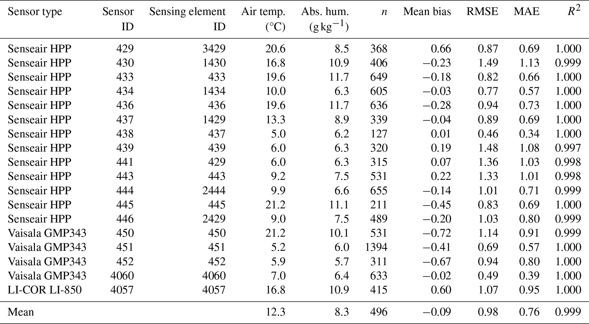
The sensors' average hourly mean root mean squared error (RMSE) was 0.98 ppm and ranged between 0.46 and 1.5 ppm, depending on which sensor was being tested (Fig. 4; Table A3). The average mean bias was −0.09 ppm, but the average mean bias also demonstrated values between −0.72 and 0.66 ppm due to sensor variation. The calculation of the RMSE error statistic, which covers both systematic (bias) and random components, can be interpreted as the average uncertainty in the estimators' (the sensors') predictions. The measurement uncertainty of approximately 1 ppm, as determined during testing, can be confidently translated to field conditions because of the design of the testing procedure.

Figure 4 Hourly CO₂ error statistics of the sensors that were exposed to parallel measurements with a high-precision reference gas analyser at the Dübendorf-Empa monitoring site.

The discontinued Senseair HPP sensor often performed more poorly than the commercially available Vaisala GMP343 and LI-COR LI-850 sensors. The inter-sensor variability in the Senseair HPP sensors was also higher, with some sensors displaying more measurement uncertainty than others (Table A3). This variation may have been partially caused by the variability in age or uptime because some of these sensors had been used previously for monitoring in other studies (see Müller et al., 2020) or differing environmental conditions during the testing period. Furthermore, the Senseair HPP sensor was a prototype, possibly resulting in larger variations in the product. However, because of the irregular number of each sensor type, additional sensor units would need to be used to confirm these apparent patterns and not over interpret the rather small differences observed among the different sensor models.

Scatterplots of hourly means (Fig. 5) demonstrated that all three sensor types displayed excellent CO₂ measurement quality and linearity across the detected ambient CO₂ range. The scatterplots also show the importance of data processing and the improvements in measurement performance in both bias and dispersion dimensions that were achieved due to the application of correction and calibration processes (moving sequentially from the top to bottom panels in Fig. 5). In general, the Senseair HPP sensors displayed more dispersion around the reference observations and, therefore, a larger measurement error than the other two sensor models. A somewhat surprising observation was that, despite the LI-COR LI-850 measuring and reporting water vapour directly, a small water-induced response was still experimentally confirmed. Achieving the measurement performance shown in Fig. 4, Table A3, and Fig. 5 was only possible with these NDIR sensors with the utilisation and careful handling of reference gases, which is not feasible for many other atmospheric gases – including the family of reactive gases (and particulates) that are important for air quality.

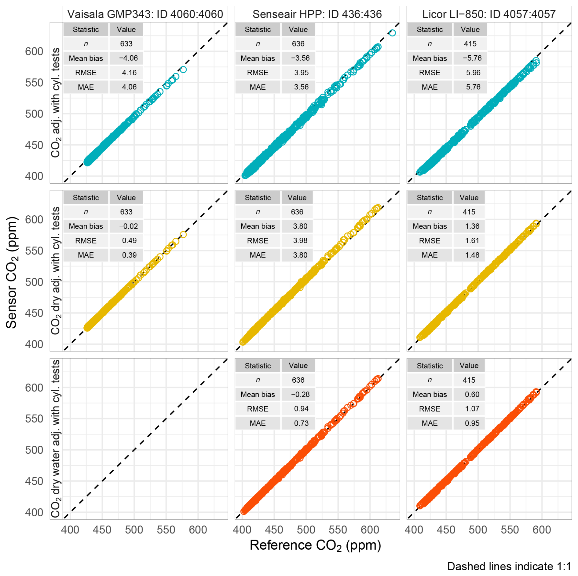
Figure 5 Hourly CO₂ means for selected sensors for the three sensor models used in the ZiCOS-M network during intercomparison at the Dübendorf-Empa monitoring site. The improvements in measurement performance can be seen when moving from top to bottom as the data processing adjustments are applied. The Vaisala GMP343 sensors did not require a water-induced adjustment; therefore, this was not calculated and is not shown. The term “cyl.” denotes “cylinder”.

The use of reference gases increased the complexity of the measurement system and the maintenance required for the operation of the network. However, the gases were critical for achieving the reported measurement performance (Fig. 5). An alternative strategy would be to use a single gas and apply only an offset correction. A sensitivity analysis exploring this approach was conducted by withholding the high gas tests and only using the low CO₂ cylinder (≈ 400 ppm) for an offset correction. The mean RMSE and bias penalties of this approach were 1.7 and 0.8 ppm, and the corresponding medians were 0.17 and 0.12 ppm (compared to the two-gas calibration discussed above). The median penalties of using a single reference gas were rather low and may be acceptable for some monitoring applications, but the larger means demonstrate that for some of the sensors (three in this case), the sensitivities altered during the testing procedure, and thus, the second gas test was required to address this robustly. This sensitivity analysis showed that an offset correction strategy could be used in some scenarios, but the sensors' sensitivity stability should be regularly tested to ensure that large measurement performance penalties do not arise.

The intercomparison periods were also used to evaluate the effectiveness of the water vapour correction that was determined in laboratory tests under real conditions. Figure 6 shows the response of the three CO₂ sensor types to absolute humidity during their intercomparison periods. Without correcting for the water dilution effect, the values were biased low in comparison to the reference because the sensors reported CO₂ in moist air. In the case of the Senseair HPP, converting from moist to dry mole fractions (i.e. correcting for the water dilution) led to an overestimation of CO₂. Additionally, correcting for the water-induced response brought the residuals close to zero, demonstrating the importance of this additional correction.

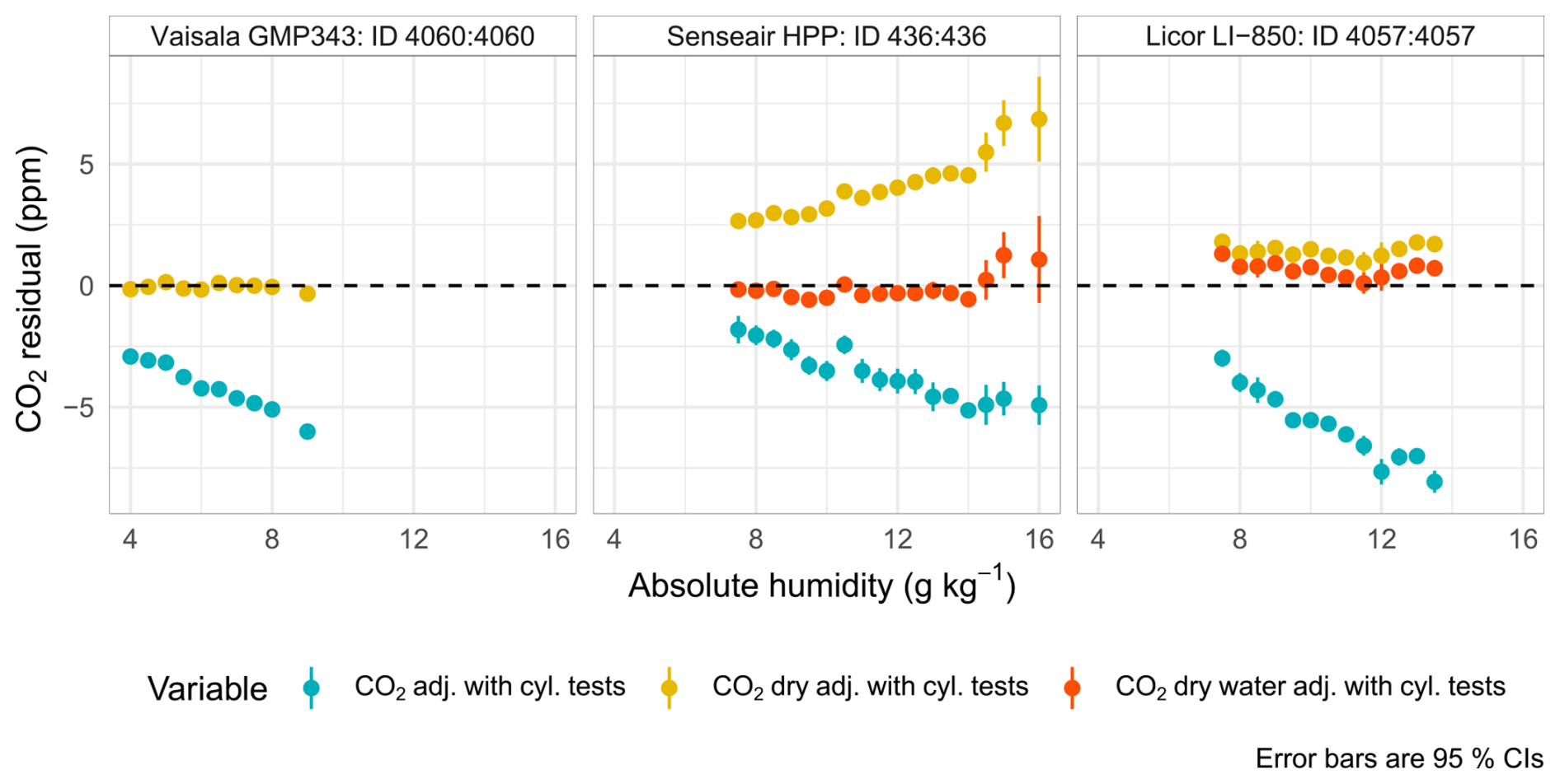
Figure 6 CO₂ residuals by sample absolute humidity (in 0.5 g kg⁻¹ bins) during parallel measurements with a high-precision reference gas analyser at the Dübendorf-Empa monitoring site. The clear influence of dilution (negative) and the water-induced response (positive) can be observed in the Senseair HPP example as can the efficacy of the post-measurement adjustments or corrections.

An hourly CO₂ measurement uncertainty of 1 ppm is comparable to other studies that report such results for CO₂ NDIR sensors (Shusterman et al., 2016; Martin et al., 2017; Kunz et al., 2018; Arzoumanian et al., 2019; Müller et al., 2020; Delaria et al., 2021; Lian et al., 2024). Direct comparisons among the various studies are difficult due to the different endpoints that were defined, variable testing or intercomparison designs, and whether the stated uncertainty or error truly represents field conditions. However, because many studies have reported rather similar results, it is likely that measurement uncertainties of ≈ 1 ppm can be expected with the current generation of CO₂ NDIR sensor products. In contrast, the World Meteorological Organization has set compatibility goals of 0.1 and 0.05 ppm for background monitoring sites in the Northern Hemisphere and Southern Hemisphere, respectively, when using state-of-the-art monitors (World Meteorological Organization, 2014). Clearly, these types of sensors are unsuitable for background monitoring sites at this time.

3.2 CO₂ variation in and around the city of Zurich

3.2.1 Site means

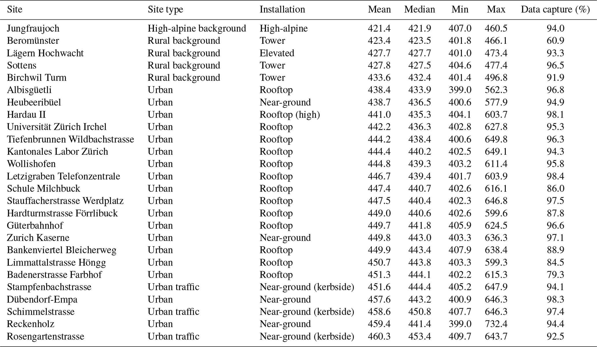
The ZiCOS-M sensor network that included 26 monitoring sites demonstrated that CO₂ was highly variable across time and the Zurich area during the monitoring period between July 2022 and July 2024. The sensor network's urban background site for the Zurich region, Birchwil Turm (Fig. 3), experienced a mean CO₂ of 434 ppm, while the highest mean CO₂ concentration of 460 ppm was found at Rosengartenstrasse (Table 3; Fig. 7). Reckenholz observed the second-highest mean CO₂ and notably was a rural, near-ground monitoring site with an inlet height of 4.2 m (Table 3). The high levels of CO₂ were driven not by anthropogenic emission activities but by strong biogenic respiration in the early hours of the morning. Dübendorf-Empa, the network's testing site was also exposed to strong biogenic forcing, with peak CO₂ occurring in the early morning during the growing seasons including spring, summer, and autumn. The processes governing these features are further explored in Sect. 3.2.2. Beromünster suffered an observation gap between late August 2023 and early February 2024 due to instrument failure and, therefore, had a lower data capture rate compared to the other sites.

Table 3 Summary statistics for the CO₂ monitoring sites between July 2022 and July 2024. The CO₂ unit is ppm, representing dry-air mole fractions, and the sites are ordered by their mean CO₂.

Figure 7 Mean CO₂ for ZiCOS-M's 26 monitoring sites between July 2022 and July 2024.

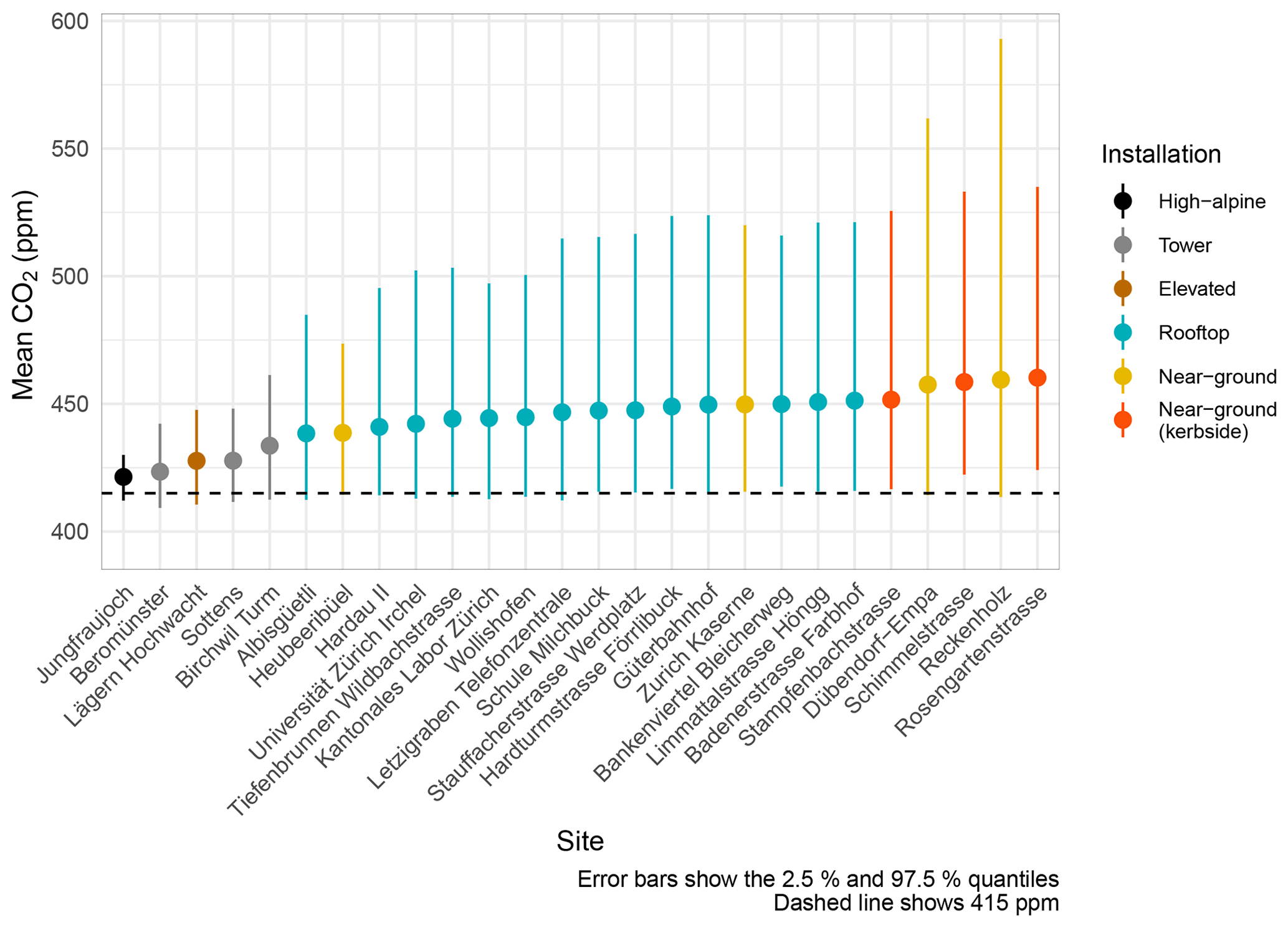
Rosengartenstrasse was the most enhanced monitoring site with respect to CO₂. Rosengartenstrasse is in the city of Zurich proper and is located in a kerbside environment next to an uphill and northbound section of an arterial road. It displayed a clear traffic-forced diurnal cycle of CO₂ during the day, as observed in other cities (Shusterman et al., 2018). The two other traffic sites located in kerbside environments – Schimmelstrasse and Stampfenbachstrasse – also experienced some of the highest CO₂ of the network (Table 3; Fig. 7).

Site means for the daytime hours (local time (LT) between 10:00 and 16:00) are also provided in Fig. A6. The gradient between background and rooftop sites was, on average, about 25 ppm for daily means but only 15 ppm for daytime means. For the kerbside locations Rosengartenstrasse and Schimmelstrasse, the gradient was about 30 ppm in both cases, suggesting that their concentrations are primarily determined by their proximity to traffic and less so by atmospheric dispersion dynamics.

When considering only the rooftop sites with measurement heights between 13.5 and 114 m (Table 2), the daily means ranged from 438 ppm at Albisgüetli to 451 ppm at Badenerstrasse Farbhof (Table 3), a mean gradient within the city of 13 ppm. For daytime means, the gradients were only about half this magnitude, but they were still sufficiently large to be reliably captured by the sensors, given their measurement uncertainty of 1 ppm (Sect. 3.1). Jungfraujoch, the high-alpine monitoring site located in the distant Bernese Alps at an elevation of 3572 m, experienced a daily mean of 421 ppm, which represented European background CO₂ during the period of monitoring. Another interesting observation is that the distant sensor site in Sottens in Vaud (western Switzerland; Fig. 2) had lower mean and median CO₂ than Zurich's regional background site Birchwil Turm, despite their comparable installation and sampling height, which suggests the source–sink dynamics across the Swiss Plateau were variable during the monitoring period.

3.2.2 Diurnal cycles and ranges

The diurnal cycle of CO₂ at the 26 sites in the ZiCOS-M network formed three broad groups reflecting different source and sink dynamics that can be classified as background, anthropogenically influenced, and biogenically forced. Background sites demonstrated minor changes in mean hourly CO₂ throughout the year, but, except for at Jungfraujoch, small amounts of morning CO₂ enhancement and afternoon reduction were present in all seasons (Fig. 8). The magnitudes of the morning CO₂ peaks were higher than those experienced in the afternoon or evening; 3-monthly definitions of seasons were used, where summer refers to the months of June, July, and August.

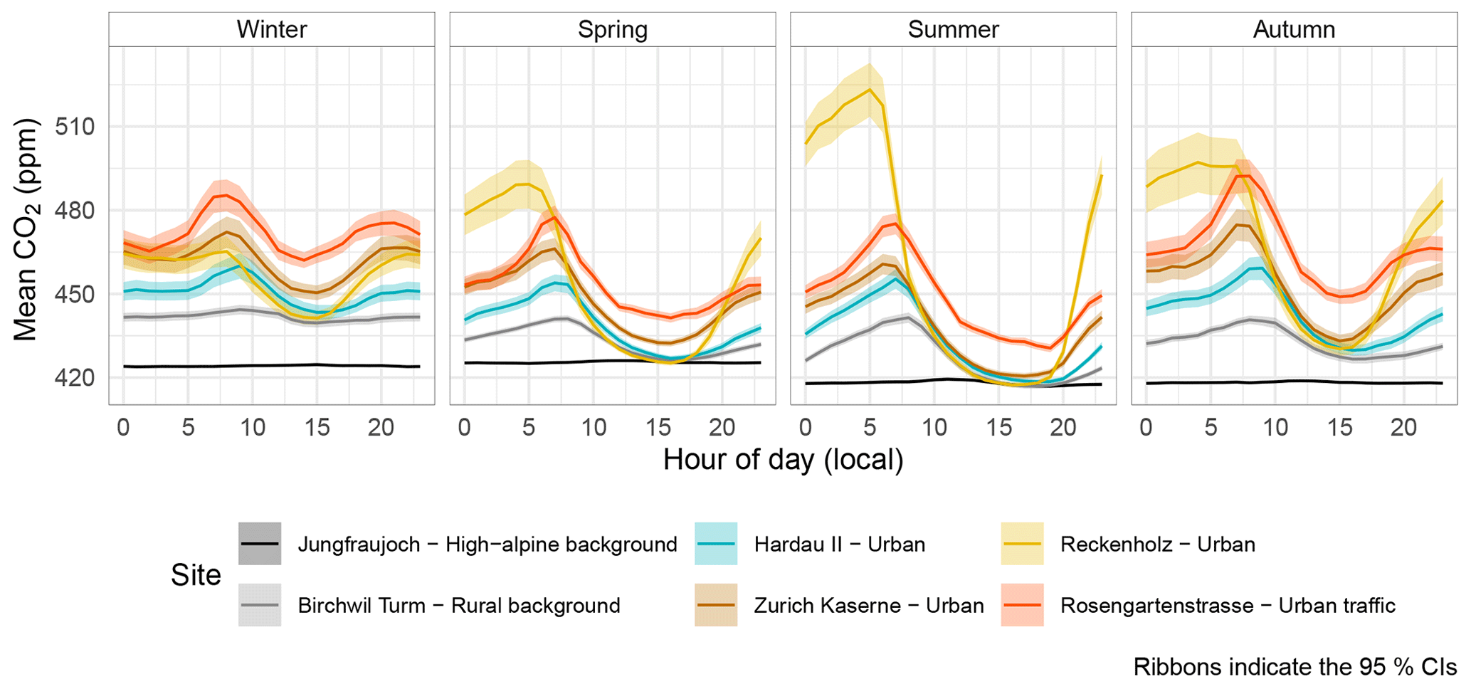
Figure 8 Seasonal CO₂ diurnal cycles for selected monitoring sites with different site type classifications between July 2022 and July 2024.

Most sensor sites were located in or around Zurich's urban area, and they showed an anthropogenically influenced diurnal cycle. These anthropogenically influenced sites were distinguished by CO₂ levels peaking in the morning (usually between 06:00 and 10:00 local time, LT), driven by traffic and other anthropogenic emission processes at these times. A combination of increased atmospheric dispersion and biogenic uptake in the early afternoon and mid-afternoon reduced CO₂ to the daily minima (Fig. 8). During summer afternoons, many of the anthropogenically influenced sites' mean CO₂ levels were below the European background at Jungfraujoch due to uptake by the local and regional biosphere, reflecting the ground level acting as a net sink in this season (Stephens et al., 2007). Outside the growing season, i.e. winter, the anthropogenically influenced sites showed a clear second peak in the afternoon or evening due to traffic and heating emissions. This was reminiscent of the diurnal cycles observed for primary air pollutants because they are co-emitted from the same sources (West et al., 2013; Fiore et al., 2015; The Royal Society, 2021) and due to the lack of strong active CO₂ sinks at this time of the year.

The Reckenholz and Dübendorf-Empa sites formed the third, biogenically forced, diurnal cycle group. This group was strikingly distinct from the other groups and was identified by peak CO₂ being reached in the early hours of the morning (04:00–06:00 LT) during the growing seasons (Fig. 8). These early-morning CO₂ peaks could exceed 730 ppm, which was higher than the peak CO₂ observed at the three kerbside monitoring sites. A combination of CO₂ emissions from ecosystem respiration processes and an extremely confined nocturnal boundary layer with no or very little advection caused these rather extreme CO₂ levels. These observations were clear demonstrations of what is known as the rectifier effect, where boundary layer dynamics and CO₂ fluxes are temporally correlated, which amplifies the diurnal variability in CO₂ beyond the magnitude expected from source–sink dynamics alone (Denning et al., 1999; Shi et al., 2020). Similar observations, such as those captured by ZiCOS-M, have been made previously, albeit to a somewhat less pronounced extent, in Switzerland (Gimmiz) (Oney et al., 2015) and Canada (Vancouver) (Crawford and Christen, 2014). Both Reckenholz and Dübendorf-Empa have significant areas of forest and crop fields in the surrounding area, and furthermore, Reckenholz is located in a shallow depression. For all three diurnal cycle groups, the daily CO₂ minima were always reached in the afternoon (between 14:00 and 16:00 LT) and showed little temporal variation among the different seasons.

To further characterise the diurnal variability across the network, the amplitudes of the mean differences between daily minimum and maximum hourly means were calculated for each season and all sites. The two biogenically forced Reckenholz and Dübendorf-Empa sites showed large diurnal ranges in all seasons, apart from winter, with diurnal ranges peaking at 106 and 81 ppm in the summer months (Fig. 9). Diurnal ranges of this magnitude were greater than those reported in previous studies, for example, Vogt et al. (2006). The extremely high values in the early-morning hours are responsible for these two sites' high mean CO₂ values, presented in Fig. 7 and Table 3. The high-alpine Jungfraujoch site is largely isolated from localised CO₂ sources and sinks and thus showed almost no diurnal range throughout all four seasons. This contrasted with all other sites in the network, which experienced their most pronounced diurnal cycle in summer, followed by spring or autumn due to the correlated diurnal variation in boundary layer depth and natural and anthropogenic sources and sinks during these seasons. The low diurnal ranges observed in winter can be mostly explained by only anthropogenic sources being active because the climate of Zurich is such (Köppen–Geiger climate classification: Cfb; Beck et al., 2018) that plant respiration and photosynthesis drop to near zero for much of this period (Zubler et al., 2014).

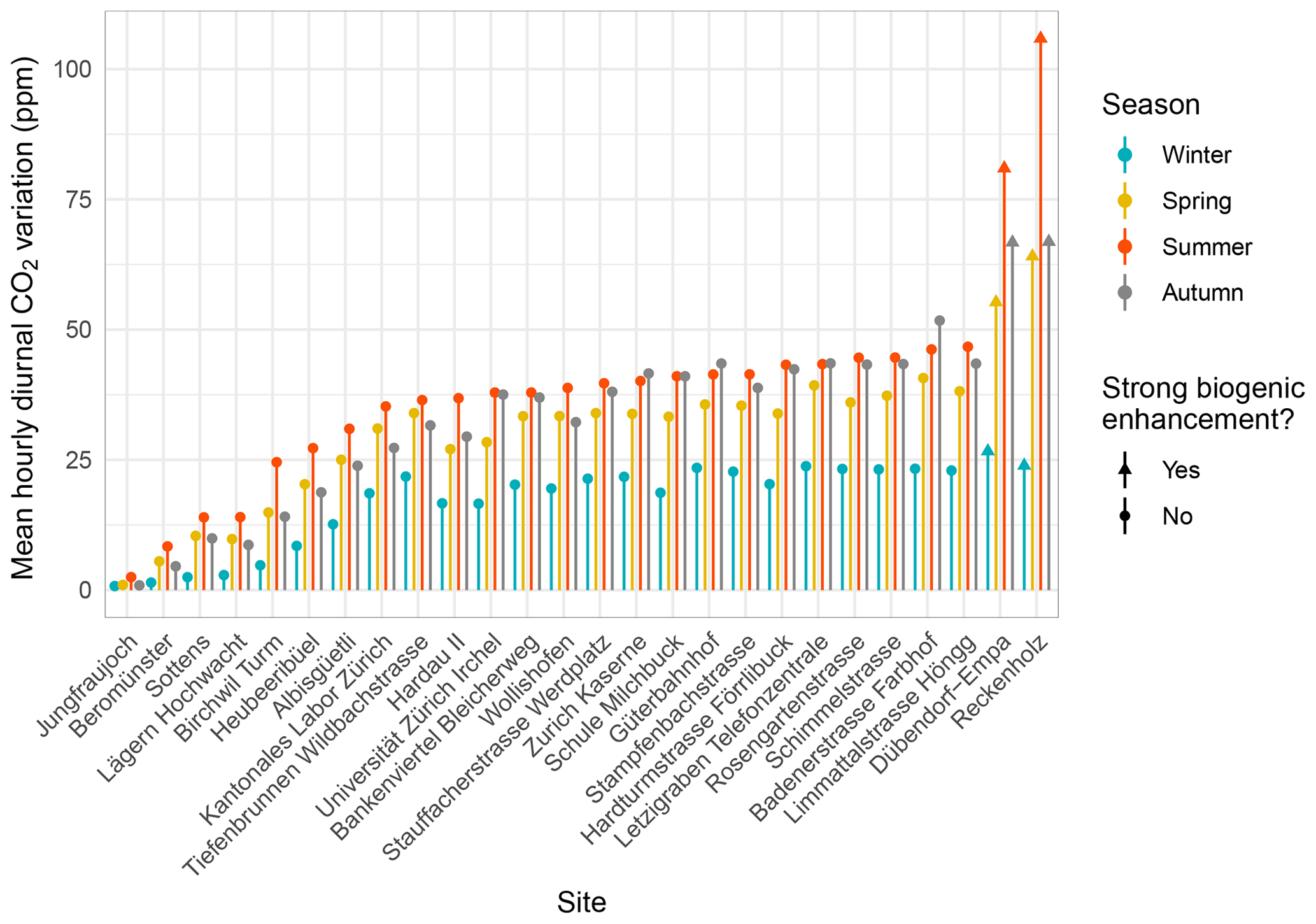
Figure 9 Mean diurnal ranges of CO₂ of minimum and maximum hourly means for four seasons for ZiCOS-M monitoring sites between July 2022 and July 2024.

3.2.3 Quantification of Zurich's urban CO₂ dome

The ZiCOS-M network was used to calculate overall and seasonal environmental increments, notably the regional CO₂ enhancement of the Swiss Plateau compared to European background mole fractions represented by Jungfraujoch and the magnitude of the city of Zurich's urban CO₂ dome, with respect to the regional background. Between July 2022 and July 2024, Zurich's regional background was on average 9.3 ppm larger than the European background and Zurich's urban CO₂ dome was enhanced by an additional 15.4 ppm above its regional background (Fig. 10). There was, however, a 12.1 ppm inter-site gradient among the rooftop monitoring sites (Fig. 7; Table 3), and this resulted in CO₂ enhancements ranging from 7.9 to 20 ppm depending on what site was considered in isolation. Urban CO₂ enhancements of such magnitudes are comparable to other urban areas where similar analyses have been conducted and reported, for example, Briber et al. (2013) and Xueref-Remy et al. (2023).

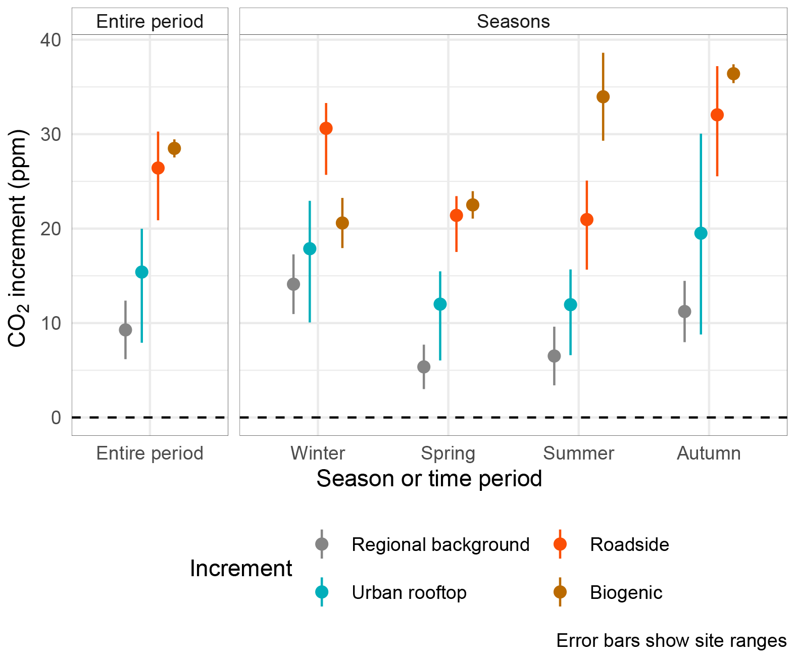
Figure 10 Daily CO₂ increments for different environments in Zurich between July 2022 and July 2024. The points indicate the groups' mean, while the error bars show the minimum and maximum of the sites within the groups.

In Zurich's roadside environments, the proximity to the principal CO₂ emission source of traffic elevated CO₂ levels by an additional 26.4 ppm enhancement above Zurich's urban dome (Fig. 10). This roadside enhancement, relative to other urban environments, remained relatively constant during winter, spring, and summer, but it did increase in autumn. This suggests that the extra roadside loading of CO₂ remained mostly unchanged throughout the year and the regional background CO₂ was generally a more important driver of observed CO₂ in Zurich and, in turn, indicates that larger-scale (European-scale) source–sink processes drive much of the variability in CO₂ observed in Zurich's urban area. On average, the biogenically forced environments experienced higher CO₂ increments (28.5 ppm) than all other environments, including those located next to the roadside (Fig. 10). However, the large increments were only present in Zurich's growing seasons, especially in summer and autumn (34 and 36.4 ppm, respectively), but only in daily means and not in daytime means, as previously discussed.

3.2.4 Zurich's regional CO₂ background

A striking feature of the network behaviour was that Zurich's regional background CO₂ was highly variable. Figure 11 shows daily means of CO₂ for the Birchwil Turm and Lägern Hochwacht regional background monitoring sites and the high-alpine site of Jungfraujoch. The figure shows the large dynamic range and pronounced temporal variability in the regional background enhancement relative to Jungfraujoch. Enhanced CO₂ was generally experienced in episodes with durations between 4 and 25 d, the longest of which was experienced in November and December 2022 (episode 6 in Fig. 11). Here, an episode was defined as CO₂ being at least 14 ppm higher than at Jungfraujoch for at least 4 sequential days. In total, 20 such episodes were identified during the monitoring period. CO₂ depletion events also occurred where Zurich's daily mean background CO₂ dropped below Jungfraujoch's, but this was rather rare and did not persist for longer than 2 d.

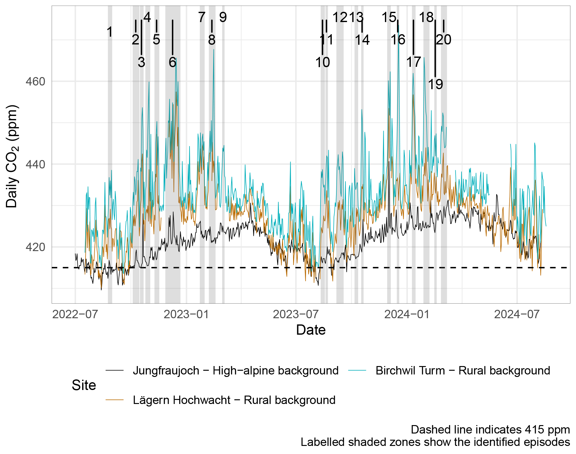
Figure 11 Daily CO₂ for two of ZiCOS-M's regional background sites and a high-alpine monitoring site between July 2022 and July 2024. Regional high-CO₂ episodes are indicated and labelled. The date format is year-month.

The 20 high-CO₂ episodes, which were objectively classified, were explored, and these episodes were not clearly related to wind speeds or wind conditions that would result in Zurich's or Winterthur's urban plumes or to emissions from Zurich's international airport being transported to the monitoring site. This suggests that Zurich's episodic high CO₂ background was driven by larger synoptic-scale processes when sink- and source-laden air masses pass over the region, as has been observed elsewhere (Hurwitz et al., 2004; Pal et al., 2020; Davis et al., 2021). Furthermore, a key observation from this analysis is that Zurich's CO₂ is not driven by a simple anthropogenic loading on top of the hemispheric (or European) background, but rather it is a function of processes acting on different scales, all of which interact to produce ambient concentrations.

To investigate these 20 episodes further, FLEXible PARTicle dispersion model (FLEXPART) (Pisso et al., 2019) footprints for a European domain were calculated using Birchwil Turm as the receptor site for the time when the sensor network was operational. This was done to determine where air masses were sourced from during the high-CO₂ episodes. To clearly visualise the origin of the air masses experienced for each episode, each episode's surface was normalised by the entire period's mean in the same way as described in Sturm et al. (2013).

The FLEXPART footprints indicated that episodes occurred in most circulation regimes, with the exception of strong flows sourced from the Atlantic Ocean (six example episodes shown in Fig. 12). Examples of northerly, southerly, westerly, and easterly flows are present, as are conditions that are consistent with extended calm conditions. These footprints and the lack of clear correlation in wind behaviour demonstrate that high background CO₂ was influenced by larger-scale processes, but high-CO₂ episodes can occur in almost any circulation regime in Zurich.

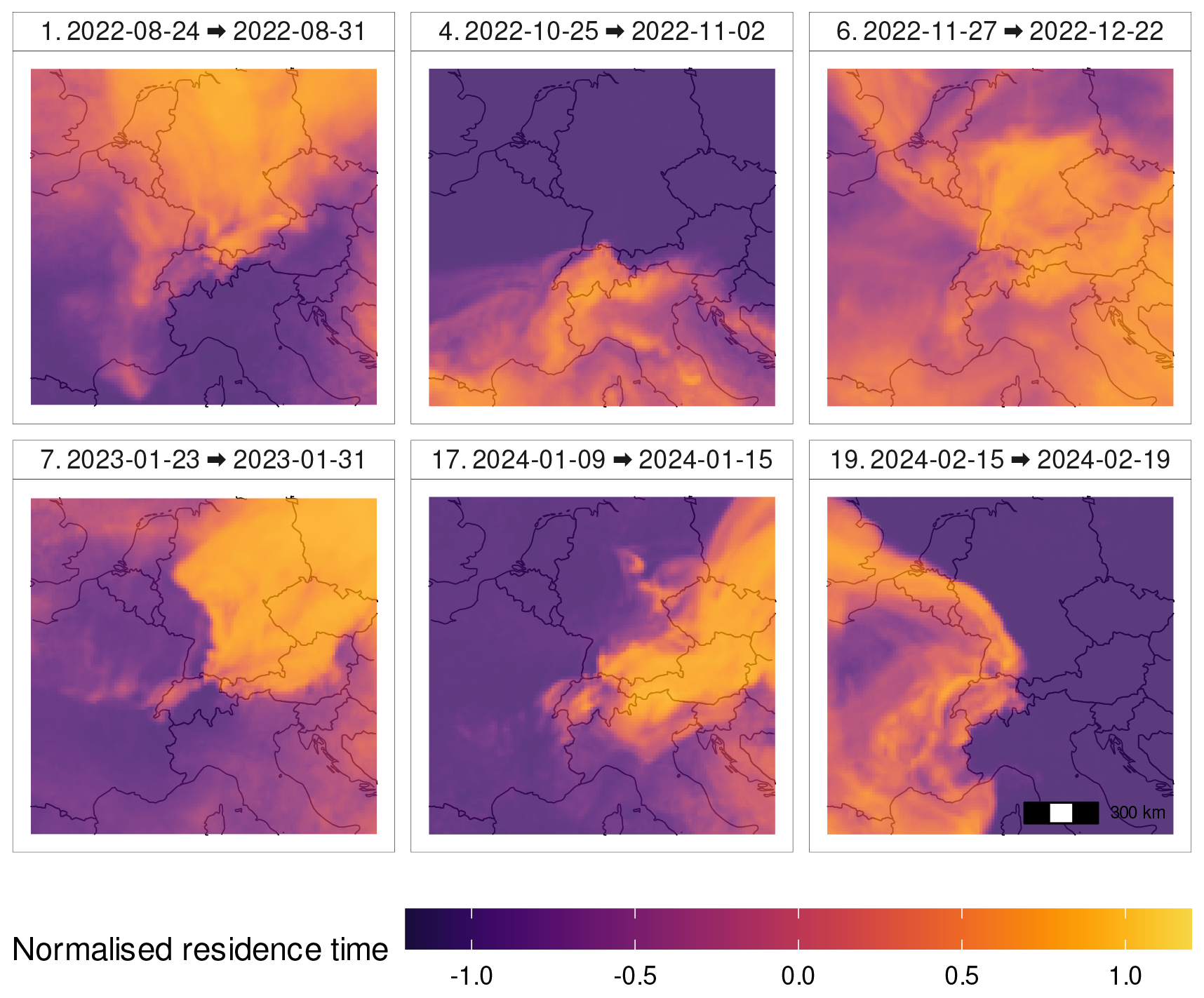
Figure 12 Normalised FLEXPART footprints (as described in Sturm et al., 2013) for Birchwil Turm for six selected high-CO₂ episodes experienced at the sensor network's regional background sites during the network's monitoring period. The date format is year-month-day.

3.2.5 A low-CO₂ urban event case study

The measurement performance of the sensors in the ZiCOS-M network was high enough to resolve local CO₂ source–sink processes. An example of this was when CO₂ dropped below regional background concentrations across the city on 3 March 2024. In Zurich on 3 March, the highest temperatures of the year to that date were experienced, peaking at 18 °C. It represented one of the first days, if not the first day, of 2024 when the biogenic uptake of CO₂ was strong due to photosynthesis. In the early afternoon, most sensor sites in the urban area experienced CO₂ levels well below those that were reported at the network's regional background monitoring sites, especially for 5 h between 13:00 and 19:00 LT (Fig. 13). The site that demonstrated this plunge in CO₂ levels the most clearly, with a difference of 17 ppm, was Universität Zürich Irchel, a rooftop monitoring site located in the north-east corner of the city (Table 3) and on the western border of the Zürichberg forest and hill (Fig. 3).

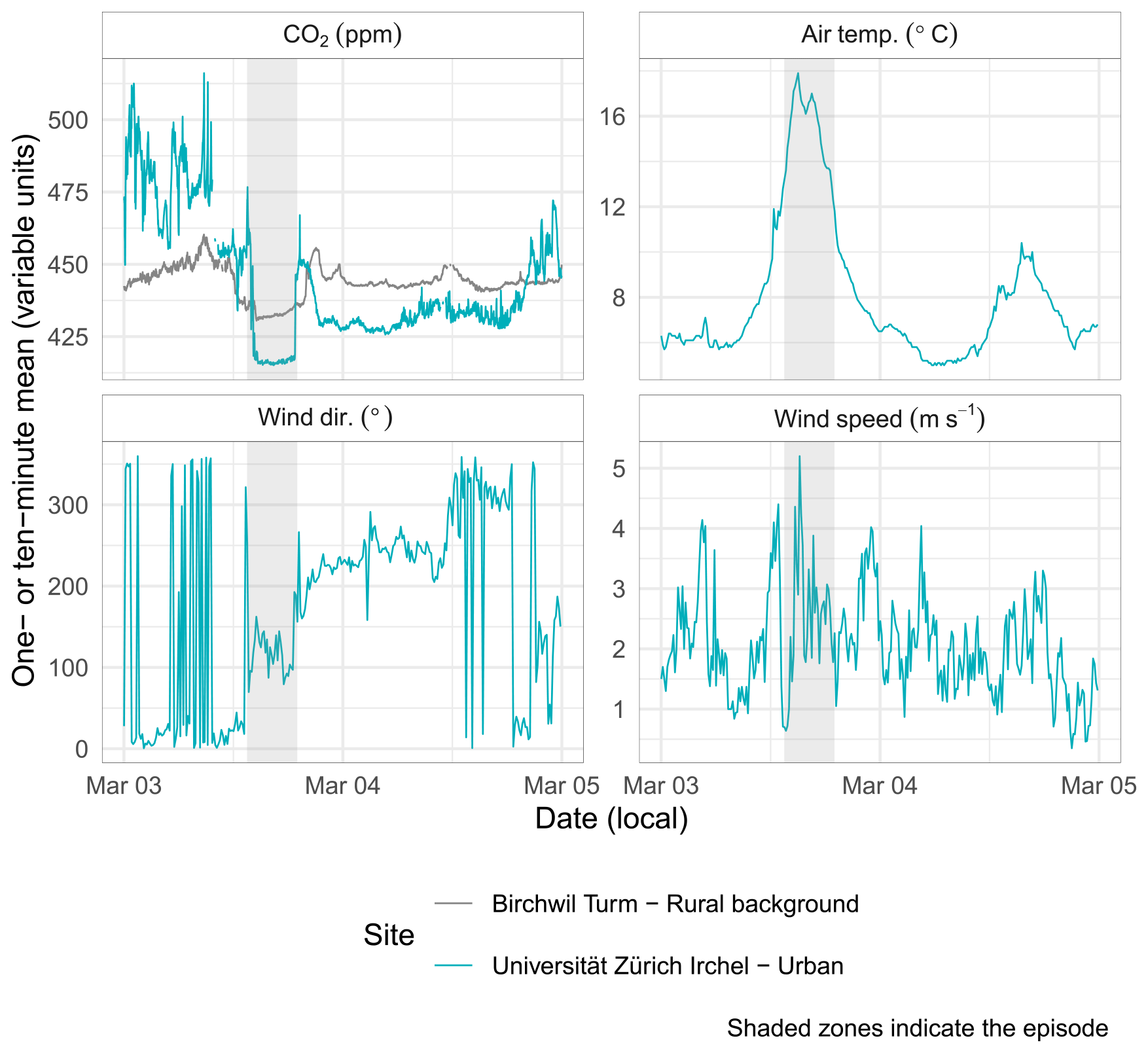
Figure 13 Time series of CO₂ and meteorological variables on 3 and 4 March 2024, demonstrating an episode where CO₂ at Universität Zürich Irchel dropped well below regional background levels due to forest air depleted of CO₂ passing over the monitoring site.

An analysis of the wind behaviour at the time of low CO₂ concentrations revealed that the episode coincided with a wind direction shift to an east-south-east direction with wind speeds above 2 m s⁻¹ (Fig. 13). This strongly suggests that air from the Zürichberg forest that was depleted of CO₂ on the first growing day of the year was being transported over the Universität Zürich Irchel site and the city in general. The depleted CO₂ air over the city took another 24 h to revert to the normal situation where CO₂ in the urban area was higher than the regional background location. The Birchwil Turm monitoring site experienced CO₂ reduction too during the afternoon of 3 March because of biogenic uptake, but the specific and local process identified around Zurich's urban area did not affect this more distant location in the same way. This case study shows that the sensor network could provide insight into very specific and local-scale processes.

4 Conclusions

The ZiCOS-M CO₂ network's sensor performance and the insights gained into atmospheric processes influencing CO₂ while the network was operational have been presented and discussed. The measurement performance of the sensors was assessed through parallel measurements with a high-precision instrument under representative field conditions. After addressing ambient pressure, water vapour, and reference gas tests, the mean uncertainty was quantified at 0.98 ppm of RMSE for hourly mean values. This level of measurement performance was high enough to confidently disentangle CO₂ gradients across Zurich's regional and urban areas.

During the monitoring period between July 2022 and July 2024, the sites' CO₂ means ranged from 433 to 460 ppm, reflecting their different surrounding environments. The sites that experienced some of the highest CO₂ were strongly influenced by biogenic respiration, with peak hourly CO₂ exceeding 730 ppm in the early hours of the morning. These levels were higher than those found in Zurich's roadside environments but only reflected biogenic respiration in certain conditions and did not reflect the full CO₂ source–sink dynamics at these biogenic sites. Zurich's urban CO₂ dome was quantified, on average, as 15.4 ppm above the regional background and ranged between 7.9 and 20 ppm when considering the individual monitoring sites. Furthermore, the sensor network showed that the processes which drove CO₂ levels acted on multiple scales, with synoptic-scale transport of CO₂-depleted or CO₂-enhanced air masses being especially important, and resulted in a very dynamic regional background that experienced several high-CO₂ episodes during the monitoring period. This illustrates that the observed CO₂ across the Zurich region was not a simple anthropogenic loading on top of a stable regional background and emphasises the importance of measurement sites placed in the surroundings of the city to characterise this background. These observations support previous studies, such as Turnbull et al. (2015).

The ZiCOS-M network provided important insights in its own right, but the observations will be used further in downstream activities utilising atmospheric inversion modelling systems, including the ICON-ART (Schröter et al., 2018; Steiner et al., 2024) and GRAMM/GRAL models (Berchet et al., 2017), to determine the city's CO₂ emissions and compare them to the established approach based on the emission inventory (Stadt Zürich, 2023b, 2024). The sensor network also contained low-cost sensors that have not been presented here. However, details and the results gleaned from the low-cost sensors are in preparation. The ZiCOS-M network acts as a good example of an environmental gas sensing monitoring network in which the measurement performance was adequate for answering a number of scientific research questions at a cost an order of magnitude lower than would be possible with contemporary state-of-the-art CO₂ reference instruments.

Appendix A: Additional figures, tables, and equations

A1 Figures

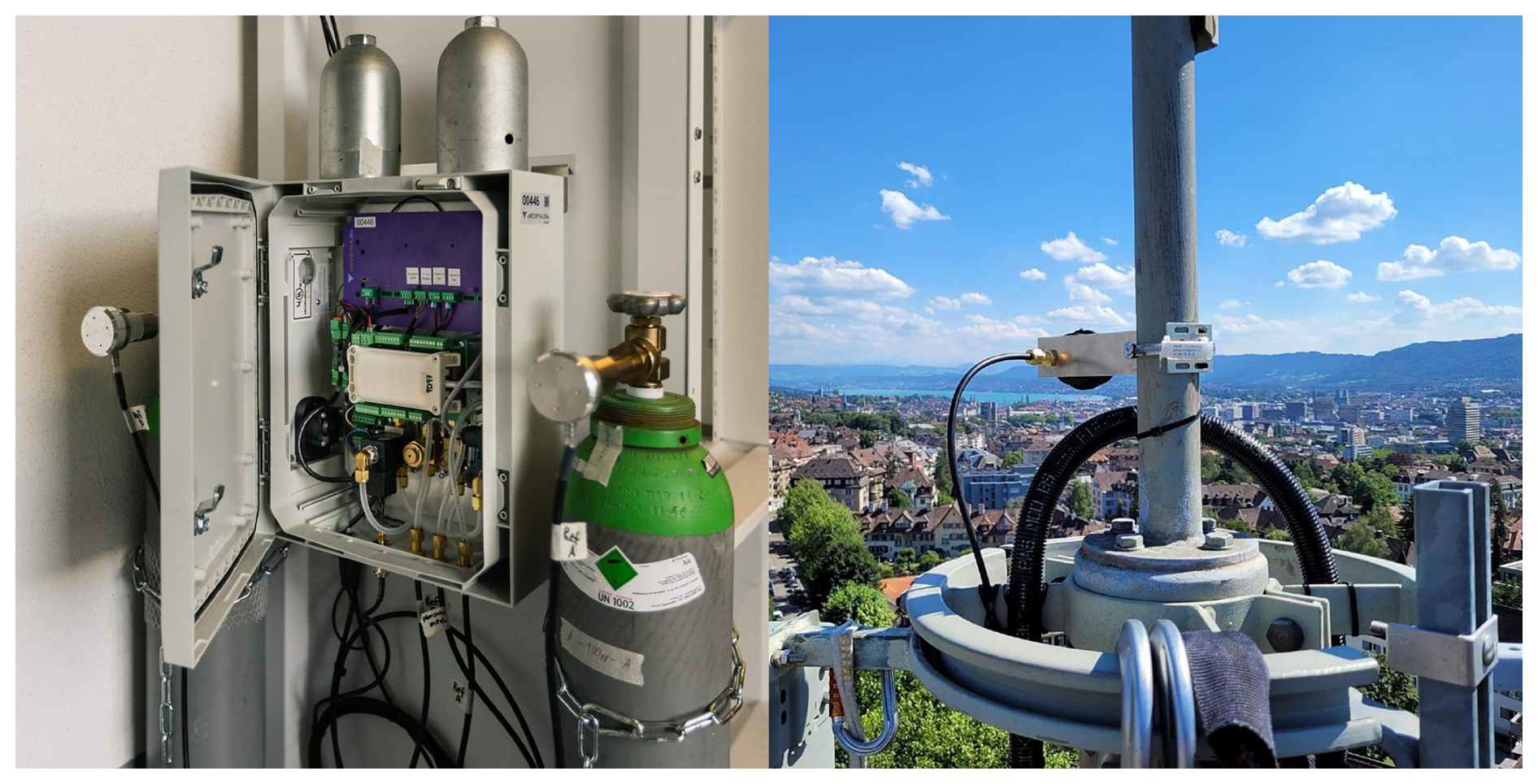
Figure A1 Examples of the CO₂ sensor's typical installation in the ZiCOS-M sensor network in the city of Zurich. The photograph on the left was taken by Pekka Pelkonen from ICOS RI.

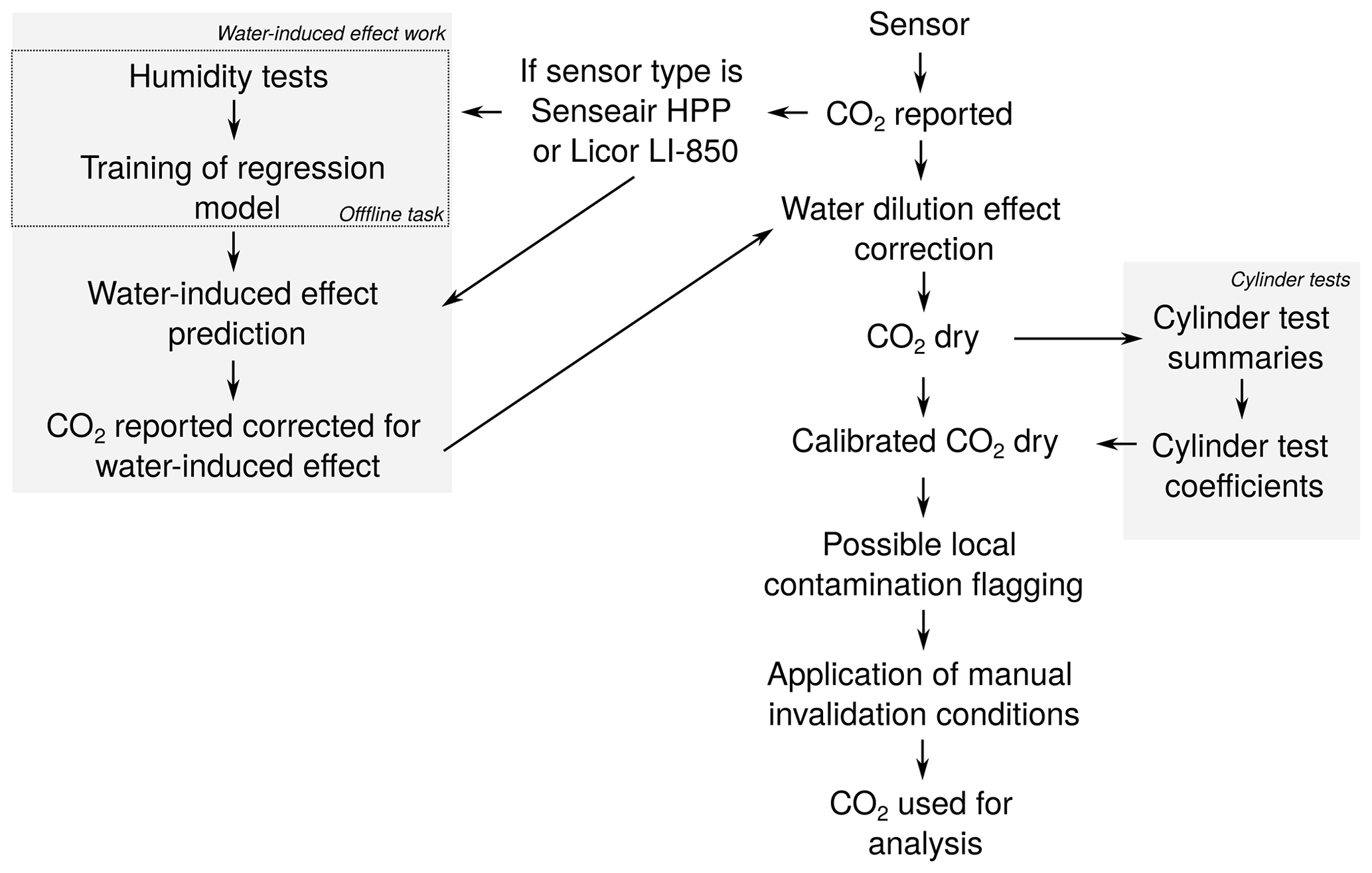
Figure A2 Schematic of the data handling steps for the sensors' CO₂ observations in the ZiCOS-M sensor network.

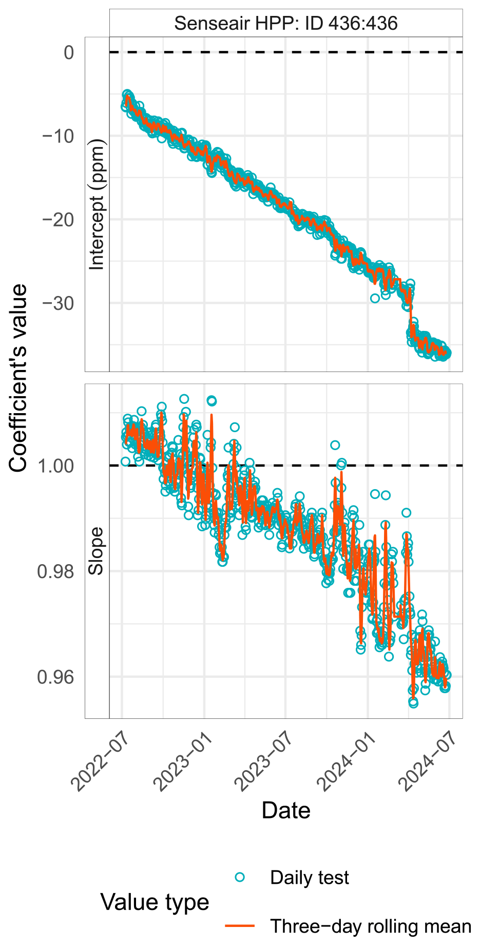
Figure A3 Slope and offset coefficients calculated from daily reference gas cylinder tests for an example sensor between July 2022 and July 2024. When applying the adjustment calculations, the 3 d rolling mean coefficients were used. This particular sensor demonstrated a decline in baseline and sensitivity during the monitoring period. The date format is year-month.

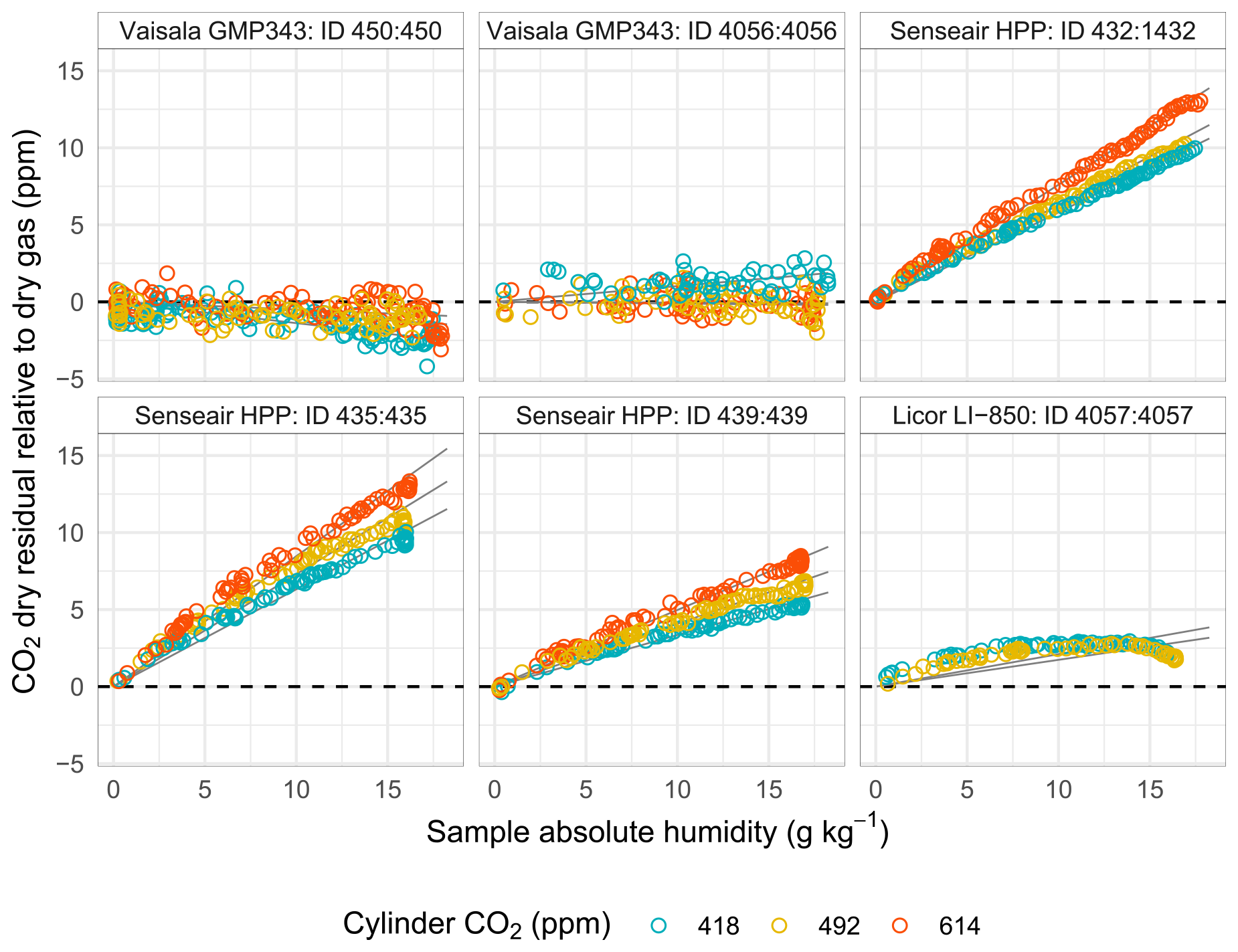
Figure A4 Examples of the water-induced response for three different types of CO₂ sensors during the decaying humidity tests. The Senseair HPP sensors strongly demonstrated the effect.

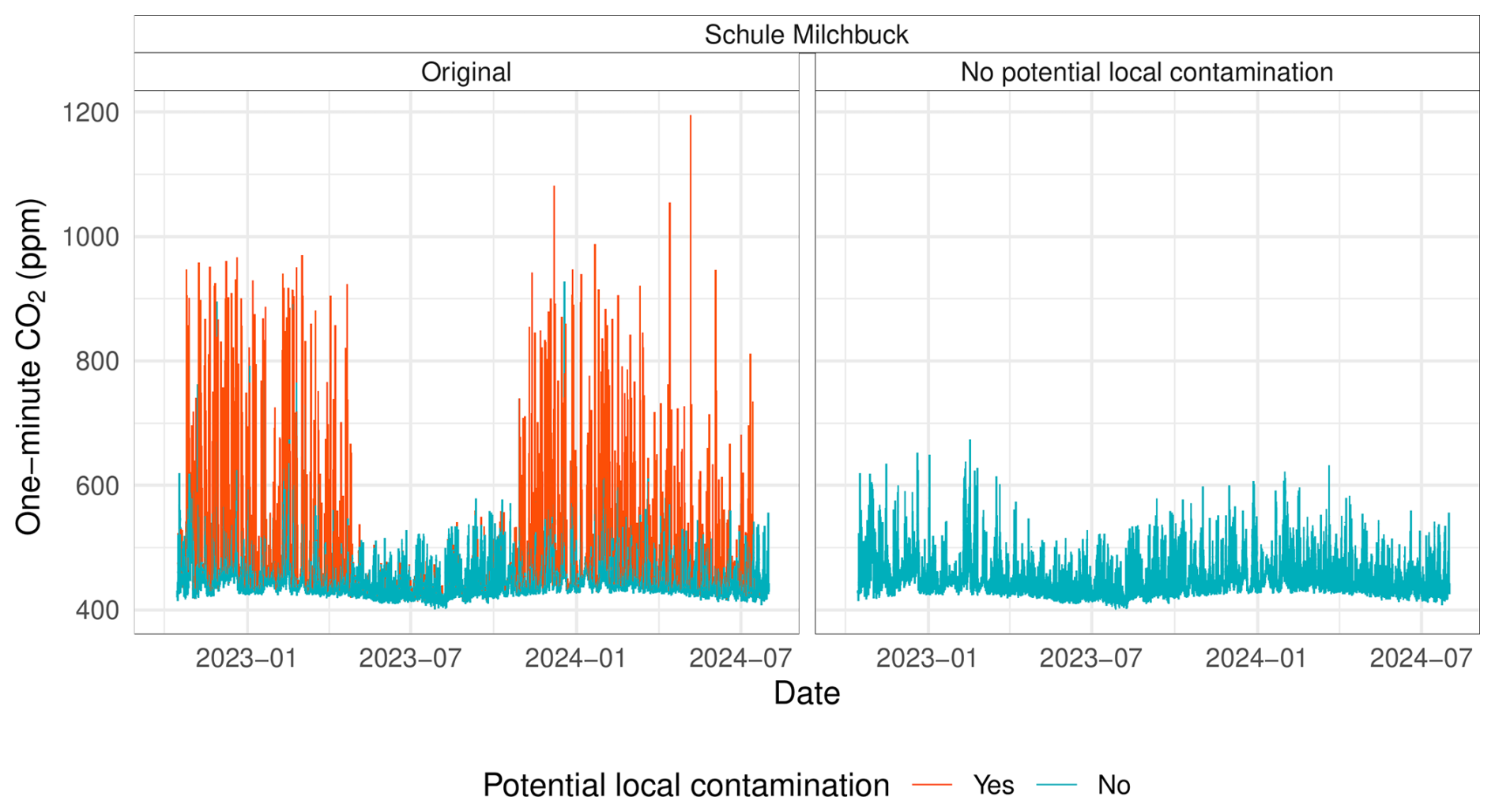
Figure A5 An example of the potential local contamination identification for a CO₂ sensor rooftop monitoring site between October 2022 and July 2024 where heating periods can be visually identified (this site is a school). The observations that were identified as contaminated by local contamination were flagged for optional handling by downstream data users. The date format is year-month.

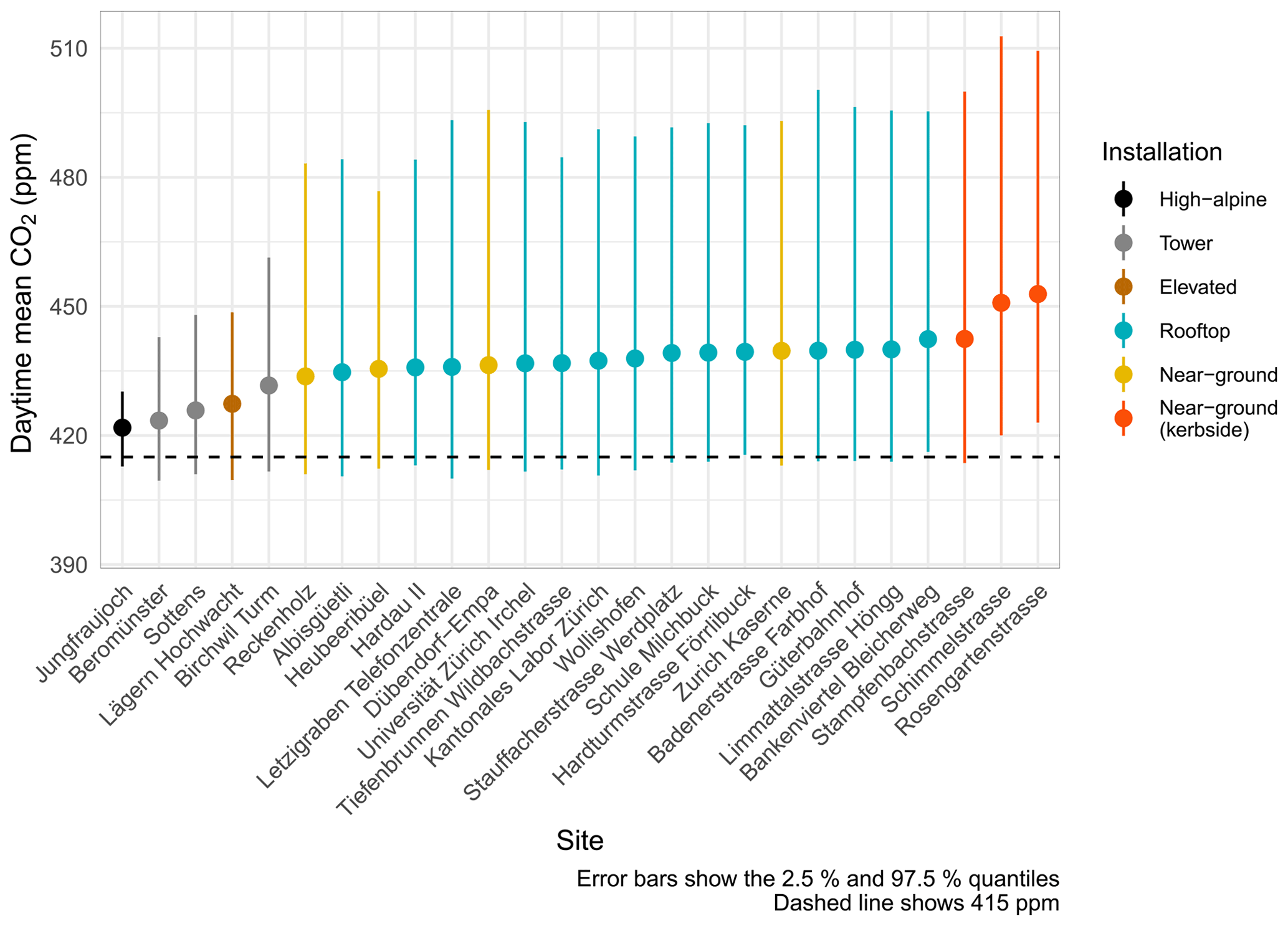
Figure A6 Mean daytime (between 10:00 and 16:00 LT) CO₂ for ZiCOS-M's 26 monitoring sites between July 2022 and July 2024.

A2 Tables

Table A1 Mid-cost sensors' parts or component makes and models.

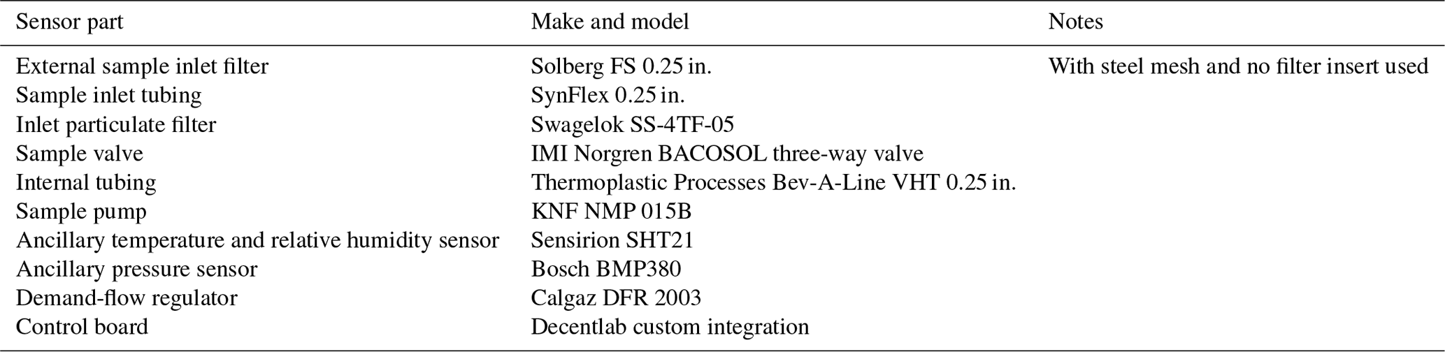
Table A2 Fraction of observations that were identified as potentially locally contaminated with an outlier detector for 14 rooftop monitoring sites.

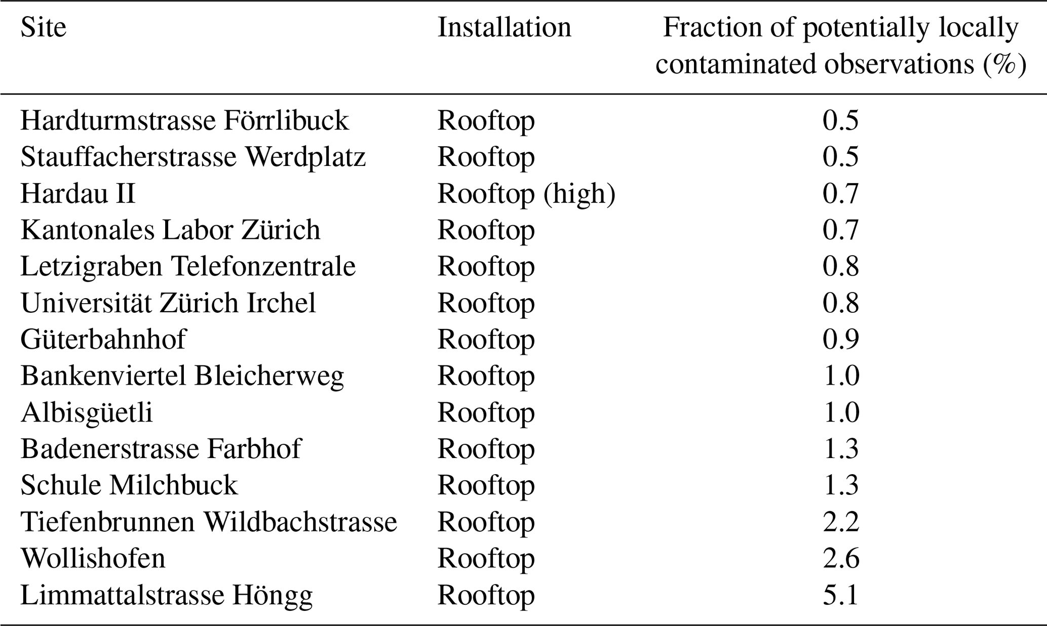
Table A3 Hourly CO₂ dry-air mole fraction error statistics of the CO₂ sensors when undergoing parallel measurements in field conditions with a high-precision gas analyser acting as ground truth. The three error statistic units are ppm. The air temperature and absolute humidity are the means for the testing duration. Sensors 438 and 445 suffered from poor data transmission during testing, so their n values are significantly lower than the target of 336 h (2 weeks). The last row shows the means of the statistics.

A3 Equations

The spectroscopic correction to address the sensors' water-induced response was conditionally applied to some sensor types in the following way:

$$\begin{array}{}\text{(A1)}& \begin{array}{rl}& {\mathrm{CO}}_{{\mathrm{2}}_{\mathrm{w}}}=\\ & \left\{\begin{array}{ll}\begin{array}{c}{\mathrm{CO}}_{{\mathrm{2}}_{\mathrm{reported}}}-({\mathrm{CO}}_{{\mathrm{2}}_{\mathrm{reported}}}\\ \cdot {\mathit{\beta }}_{{\mathrm{CO}}_{\mathrm{2}}}+w\cdot {\mathit{\beta }}_{\mathrm{w}})\end{array}& \begin{array}{c}\text{if sensor type was}\\ \text{Senseair HPP}\\ \text{or LI-COR LI-850},\end{array}\\ {\mathrm{CO}}_{{\mathrm{2}}_{\mathrm{reported}}}& \text{else},\end{array}\right.\end{array}\end{array}$$

where ${\mathit{\beta }}_{{\mathrm{CO}}_{\mathrm{2}}}$ and β_w represent slopes of multiple linear regression models that were trained on observations during humidity tests (Sect. 2.3.4). The Senseair HPP sensors' reported CO₂ required transformation to standard pressure and was done using standard atmospheric pressure (atm):

$$\begin{array}{}\text{(A2)}& \begin{array}{rl}& {\mathrm{CO}}_{{\mathrm{2}}_{\mathrm{p}}}=\\ & \left\{\begin{array}{ll}{\mathrm{CO}}_{{\mathrm{2}}_{\mathrm{w}}}\cdot \left(\frac{\mathrm{1013.25}}{P_{\mathrm{o}}}\right)& \text{if sensor type was Senseair HPP},\\ {\mathrm{CO}}_{{\mathrm{2}}_{\mathrm{w}}}& \text{if sensor type was LI-COR LI-850},\\ {\mathrm{CO}}_{{\mathrm{2}}_{\mathrm{reported}}}& \text{else}.\end{array}\right.\end{array}\end{array}$$

To compute CO₂ dry-air mole fractions, water partial pressure (P) was calculated with the August–Roche–Magnus equation (Alduchov and Eskridge, 1996; Lawrence, 2005) using temperature (T) and relative humidity (RH) observations from the sensors' sample stream, and, in turn, the water vapour mixing ratio was calculated, and the sensors' CO₂ moist air mole fractions were transformed using observed air pressure (P_o):

$$\begin{array}{}\text{(A3)}& {\displaystyle }& {\displaystyle }P={\displaystyle \frac{\mathrm{RH}}{\mathrm{100}}}\cdot \mathrm{6.1078}\cdot \exp \left({\displaystyle \frac{\mathrm{17.08085}\cdot T}{\mathrm{234.175}+T}}\right),\text{(A4)}& {\displaystyle }& {\displaystyle }{\mathrm{CO}}_{{\mathrm{2}}_{\mathrm{dry}}}={\displaystyle \frac{{\mathrm{CO}}_{{\mathrm{2}}_{\mathrm{p}}}}{(\mathrm{1}-\frac{P}{P_{\mathrm{o}}})}}.\end{array}$$

Finally, CO₂ dry-air mole fractions were calibrated with slopes (β_cylinder) and offsets (α_cylinder) calculated from reference gas tests conducted every 25 h:

$$\begin{array}{}\text{(A5)}& {\mathrm{CO}}_{{\mathrm{2}}_{\mathrm{dry}\mathrm{cal}}}={\mathrm{CO}}_{{\mathrm{2}}_{\mathrm{dry}}}\cdot {\mathit{\beta }}_{\text{cylinder}}+{\mathit{\alpha }}_{\text{cylinder}}.\end{array}$$

The product of these transformations was CO₂ dry-air mole fractions calibrated to the WMO X2019 calibration scale (Hall et al., 2021).