Insights into ozone pollution control in urban areas by decoupling meteorological factors based on machine learning

Ozone (O₃) pollution is posing significant challenges to urban air quality improvement in China. The formation of surface O₃ is intricately linked to chemical reactions which are influenced by both meteorological conditions and local emissions of precursors (i.e., NO_x and volatile organic compounds, VOCs). When meteorological conditions deteriorate, the atmosphere's capacity to cleanse pollutants decreases, leading to the accumulation of air pollutants. Although a series of emission reduction measures have been implemented in urban areas, the effectiveness of O₃ pollution control proves inadequate. Primarily due to adverse changes in meteorological conditions, the effects of emission reduction are masked. In this study, we integrated a machine learning model, an observation-based model, and a positive matrix factorization model based on 4 years of continuous observation data from a typical urban site. We found that transport and dispersion impact the distribution of O₃ concentration. During the warm season, positive contributions of dispersion and transport to O₃ concentration ranged from 12.9 % to 24.0 %. After meteorological normalization, the sensitivity of O₃ formation and the source apportionment of VOCs changed. The sensitivity of O₃ formation shifted towards the transition regime between VOC- and NO_x-limited regimes during the O₃ pollution event. Vehicle exhaust became the primary source of VOC emissions after “removing” the effect of dispersion, contributing 41.8 % to VOCs during the pollution periods. On the contrary, the contribution of combustion to VOCs decreased from 33.7 % to 25.1 %. Our results provided new recommendations and insights for implementing O₃ pollution control measures and evaluating the effectiveness of emission reduction in urban areas.

1 Introduction

Ozone (O₃) plays a significant role in atmospheric oxidation and global climate. It is also considered one of the major atmospheric pollutants. A high concentration of surface O₃ is harmful to human health, such as causing respiratory diseases and even cancer (Cohen et al., 2017; Monks et al., 2015). In recent years, China has been in a stage of rapid economic development, accompanied by the emergence of various air pollution problems due to industrialization and urbanization (Zhang et al., 2012). In order to deal with the air pollution, the Chinese government has issued some control policies, such as the Clean Air Action Plan in 2013 (Chinese State Council, 2013) and the Blue Sky Protection Campaign in 2018 (Chinese State Council, 2018). These policies have resulted in reductions in the concentrations of particulate matter (PM), nitrogen dioxide (NO₂), and sulfur dioxide (SO₂) (Zheng et al., 2018). However, O₃ pollution has become increasingly serious, especially in typical urban clusters such as Beijing–Tianjin–Hebei (BTH), the Yangtze River Delta (YRD), and the Fenwei Plain (FWP). In 2022, the 90th percentile of maximum daily 8 h average (MDA8) O₃ was 179 µg m⁻³ in the BTH, 162 µg m⁻³ in the YRD, and 167 µg m⁻³ in the FWP, 4.7 %, 7.3 %, and 1.2 % higher than that in 2021, respectively (Ministry of Ecology and Environment of China, https://www.mee.gov.cn/hjzl/dqhj/qgkqzlzk/, last access: 31 January 2025). Frequent O₃ pollution events have attracted the attention of the public and the government. Surface O₃ is mainly formed by the photochemical reactions of volatile organic compounds (VOCs) and nitrogen oxides (NO_x = NO + NO₂) (Atkinson, 2000). The emissions of precursors effectively affect the change in O₃ concentration (Tan et al., 2018). The sources of VOCs are complex and widespread, making it challenging to control emissions (Miller et al., 2002; Borbon et al., 2013). Meteorological conditions can directly or indirectly affect O₃ concentration (Liu and Wang, 2020; Zhang et al., 2015; Gao et al., 2021; Han et al., 2020). Wind and boundary layer height influence the diffusion of the concentrations of O₃ and its precursor. Poor dispersion can result in a decrease in atmospheric environmental capacity, making O₃ pollution events more likely to occur even with low precursor emissions. High ultraviolet radiation and temperature promote photochemical reactions of O₃ formation (Yang et al., 2019). In addition, O₃ can be transported over long distances due to its the long atmospheric lifetime, which can cause regional O₃ problems (Han et al., 2019). In short, the O₃ concentration is nonlinearly affected by meteorological conditions, emissions of precursors, and chemical reactions (Fu et al., 2019; Hu et al., 2021; Zhang et al., 2022, 2024).

Li et al. (2020) discovered that approximately one-third of the growth of O₃ concentration in summer in China was attributed to meteorological conditions. This indicated that the reduction of air pollutant concentrations due to the control policies may be offset by the deterioration of meteorological conditions. Therefore, decoupling meteorological factors from temporal concentration series of atmospheric pollutants is helpful to assess the impact of clean air actions. At present, many mathematical statistical methods have been developed to “remove” the influences of meteorological factors. The technique for predicting air pollutant concentrations under randomly selected meteorological parameters was first introduced by Grange et al. (2018). Weng et al. (2022) found that the temperature near the surface 2 m, the downward radiation flux of the surface and the relative humidity were the most important meteorological factors to affect O₃ concentration in China by applying two machine learning algorithms (ridge regression and random forest regression). Mousavinezhad et al. (2021) employed the Kolmogorov–Zurbenko (KZ) filter method and found that meteorological factors played the dominant role in O₃ formation in four typical urban agglomerations in China. Guo et al. (2022) used the random forest method to obtain the characteristics of air pollution in 12 megacities in China from 2013 to 2020 and carried out a comprehensive assessment of the actual impact of the national clean air action. Compared to traditional statistical methods, machine learning models perform better at removing meteorological effects from concentration data.

In response to severe O₃ pollution, a series of emission reduction measures targeting O₃ precursors were implemented in urban areas. However, the effectiveness of controlling O₃ pollution fell short of expectations. According to previous studies, O₃ formation in urban areas was more sensitive to VOCs (Feng et al., 2019; Wang et al., 2023), with anthropogenic emissions of VOCs playing a dominant role (Ahmad et al., 2017). Understanding the sensitivity of O₃ formation and the source characteristics of VOCs is helpful to design effective strategies to control O₃ pollution. The observation-based model (OBM), positive matrix factorization model (PMF), and air quality model are commonly used to analyze the causes of O₃ pollution and provide theoretical support for reducing O₃ precursors. However, the results of the OBM and PMF, which rely on observed data, may be influenced by fluctuations in meteorological conditions, potentially introducing bias. Wu et al. (2023) developed initial concentration-dispersion normalized PMF (ICDN-PMF) to reflect the changes in source emissions of VOCs in Qingdao. The results proved that the contribution of solvent use was overestimated due to air dispersion during O₃ pollution. Additionally, the actual effectiveness of emission reduction measures can also be obscured by unfavorable meteorological conditions. In this study, we applied the random forest (RF) method proposed by Grange et al. (2018) to remove the dispersion and transport effects on O₃ concentration, as well as the dispersion effect on precursors in Hangzhou from 2019 to 2022. After meteorological normalization, the concentrations of VOCs were imported into the OBM and PMF to obtain the sensitivity of O₃ formation and the contributions of emission sources, providing more accurate results. The interplay of meteorological and local factors on O₃ pollution can be evaluated effectively and comprehensively using this method. Our results emphasized the importance of decoupling the meteorological effects of transport and dispersion for understanding the mechanisms of local O₃ formation and devising appropriate emission reduction measures.

2 Methods

2.1 Observation data

The online hourly observation data from 2019 to 2022 were measured by the Zhejiang Ecological and Environmental Monitoring Center (30.29° N, 120.13° E). This station was located in the urban area of Hangzhou, Zhejiang Province, surrounded by residential and commercial areas. The dataset of air pollutants included O₃; NO₂; and 98 different kinds of VOCs detected by the gas chromatography system, including 29 alkanes, 11 alkenes, 1 alkyne, 16 aromatics, 28 halohydrocarbons, 12 oxygenated VOCs (OVOCs), and 1 acetonitrile. The online gas chromatography system was equipped with a mass spectrometer and flame ionization detector (GC-MS/FID) (ZF-PKU-VOC1007, Beijing Pengyu Changya Environmental Technology Co. Ltd., China), which used a dual gas path separation method. VOCs with low carbon numbers (C₂–C₅) were measured by a FID, while VOCs with high carbon numbers (C₅–C₁₀) were detected by a MS. NO₂ and O₃ were measured by a commercial instrument (Model 42i/42iTL and Model 49i, Thermo Scientific, USA). The meteorological parameters measured included temperature (T), relative humidity (RH), atmospheric pressure (P), wind speed (WS), and wind direction (WD), which were measured by the WS500-UMB instrument manufactured by Lufft Corporation. In addition, we used the meteorological data from the ERA5 reanalysis product (Hersbach et al., 2020), such as boundary layer height (BLH) and ultraviolet radiation B (UVB). The EAR5 meteorological data are spatial grid data with a resolution of 0.25° × 0.25°, available at https://cds.climate.copernicus.eu/datasets (last access: 31 January 2025). The back trajectories were calculated backwards in time for 24 h and started 500 m above ground level using the Hybrid Single Particle Lagrangian Integrated Trajectory (HYSPLIT) model (Stein et al., 2015). The meteorological data from the Global Data Assimilation System (GDAS) with a horizontal resolution of 1° longitude × 1° latitude were adopted in the trajectory model. The back trajectories were then clustered into five clusters using the Euclidian distance. Clusters of backward trajectories have been widely employed to represent the main directions of air masses at monitoring sites (Song et al., 2021).

2.2 Meteorological normalization method

Random forest is a versatile classifier that comprises multiple decision trees, applicable to classification, regression, and dimension reduction problems. When constructing each tree in the RF model, a dataset of the same size is selected for training, potentially containing duplicates. This sampling method, which involves putting instances back into the dataset, is referred to as bootstrap. At each node, the optimal segmentation is calculated by randomly selecting a subset of features from the entire set. The RF model describes the relationship between the time series of atmospheric pollutant concentrations and their corresponding feature. We constructed the RF model based on original datasets, which contained air pollutant variables (O₃, NO₂, total non-methane hydrocarbon compounds (NMHCs), and 98 VOC species), time variables (trend, hour, weekday, month, and day of year), and meteorological variables (T, RH, P, WS, WD, UVB, BLH, and cluster). In the RF model, the air pollutants were the response variables, while the explanatory variables included time variables representing source emissions and meteorological variables representing physical and chemical processes. Time variables such as day of year, month, weekday, and hour are used to indicate the seasonal, weekly, and daily cycles of emission intensity (Dai et al., 2023a, b; Vu et al., 2019). The parameter “trend” can indicate the long-term changes in air pollutant concentrations resulting from the implementation of policy measures (Vu et al., 2019). Environmental regulations and policies aimed at reducing pollutant emissions were implemented during specific periods, and their effects became apparent in the long-term trends. Therefore, the trend not only reflected changes in emission sources closely related to activity levels but also represented the long-term variations in air pollutants caused by the enforcement of policies and regulations. The parameter trend was calculated using Eq. (1):

$$\begin{array}{}\text{(1)}& \mathrm{trend}={\mathrm{year}}_i+{\displaystyle \frac{t_{\mathrm{JD}}-\mathrm{1}}{N_i}}+{\displaystyle \frac{t_{\mathrm{H}}}{\mathrm{24}{N}_i}},\end{array}$$

where N_i is the number of days in the year_i (year_i is from 2019 to 2022), t_H is hour time (0–23, referring to 00:00–23:00), and t_JD is the day of the year (1–365) (Carslaw and Taylor, 2009).

Temperature was a key factor influencing the rate of chemical reactions, with higher temperatures typically promoting the photochemical reactions that generate O₃. UVB served as the driving force for the photochemical reactions, directly impacting O₃ formation. Additionally, humidity played an important role in the chemical processes involved in O₃ formation. Therefore, T, RH, and UVB were identified as the key features associated with atmospheric photochemical reactions. WS influences the dispersion of atmospheric pollutants. At high wind speeds, air pollutants tended to be dispersed, while low wind speeds resulted in local pollutant accumulation, leading to increased concentrations. WD determined the dispersion path of atmospheric pollutants. BLH was a critical factor affecting the vertical dispersion of pollutants. A higher boundary layer allowed pollutants to disperse more effectively into the upper atmosphere, reducing surface concentrations, whereas a lower boundary layer resulted in pollutant accumulation near the ground. Thus, WS, WD, and BLH were regarded as the features of atmospheric physical dispersion on a local scale. The cluster can serve as a feature of transport from remote regions.

There are approximately 32 856 valid data with a time resolution of 1 h. The RF model was trained using a forest of 1000 trees. Training the datasets of the RF model was conducted using 80 % of the original datasets, and the remaining 20 % were selected for testing. Correlation coefficients (r²), root-mean-square error (RMSE), FAC2 (fraction of predictions with a factor of 2), mean bias (MB), mean gross error (MGE), normalized mean bias (NMB), normalized mean gross error (NMGE), coefficient of efficiency (COE), and index of agreement (IOA) were used to evaluate model performance (Table S2 in the Supplement). Based on previous related research, these statistical measures indicated that the model performed well (Emery et al., 2017; Henneman et al., 2017; Vu et al., 2019).

The process of meteorological normalization involved replacing the original meteorological variables with those randomly resampled from the observation dataset and using the established RF model to predict atmospheric pollutant concentrations under different meteorological conditions. The resampling of meteorological variables was conducted over the 2-week period before and after the selected date, with the resampled hours remaining constant. This approach effectively preserved the seasonal and diurnal variations in the response variables (Vu et al., 2019). The resampling and prediction process was repeated 1000 times to generate 1000 predicted pollutant concentrations. The average values were taken as the final meteorologically normalized concentrations. In the meteorologically normalization process of O₃ concentration, meteorological variables such as WS, WD, BLH, and the cluster, which signify dispersion and transport, were randomly sampled. In the case of O₃ precursors, namely NO₂ and NMHCs, resampling was exclusively applied to WS, WD, and BLH. NO₂ and NMHCs have short atmospheric lifetimes, making them less susceptible to the influence of regional transport over large scales (Wang et al., 2023). To take into consideration that some NMHCs have relatively long lifetimes (such as acetylene), the cluster was incorporated as an explanatory variable in the RF model. For NMHCs with different lifetimes, the feature importance of the cluster was relatively low (around 1 %). Therefore, it can be approximated that NMHCs were primarily influenced by dispersion effects within the uncertainty. Feature importance was used to reflect the overall significance of explanatory variables in the RF model (Yang et al., 2023). The importance was typically represented as an array, where each value corresponded to the importance score of a specific feature. These scores usually range from 0 to 1. The higher importance score indicated that the feature had a stronger predictive capability for the response variable. The RF model was constructed using R “deweather” packages developed by Carslaw (https://github.com/openair-project/deweather, last access: 1 February 2025).

2.3 Observation-based model

An observation-based model is used in this study to simulate the formation of O₃. The model is based on Regional Atmospheric Chemical Mechanisms version 2 (RACM2) updated with a detailed isoprene oxidation mechanism (Goliff et al., 2013). As a 0-D model, this model incorporates dilution mixing within the boundary layer. However, vertical or horizontal transport of the air mass is not considered in this model. Detail of the observation-based box model can be found in Tan et al. (2017). The photolysis frequencies (J values) were calculated using the Tropospheric Ultraviolet and Visible (TUV) model (Wolfe et al., 2016). Model calculations were constrained to measured trace gases, including inorganic species (NO₂ and O₃) and organic species (VOCs). In addition, physical parameters like J values, temperature, pressure, and relative humidity were also constrained to measured values. The empirical kinetic modeling approach (EKMA) serves as a sensitivity test for the OBM. The EKMA curve offers a means to quantify intricate nonlinear relationships among O₃, NO_x, and VOCs, which can be used as a theoretical basis for designing O₃ pollution reduction strategies (Tan et al., 2018). In this study, a total of 30 emission scenarios were established for both NO_x and anthropogenic VOCs. Subsequently, O₃ concentrations resulting from changes in these precursor emissions were simulated across 900 scenarios. The EKMA curve was plotted according to the O₃ formation rate under different VOCs and NO_x conditions.

2.4 Positive matrix factorization

The positive matrix factorization model is based on a large number of data to estimate the compositions and contributions of emission sources (Paatero and Tapper, 1994). The PMF model is widely used for VOC source apportionment (Song et al., 2021; Yuan et al., 2010). In the PMF model, it is assumed that the pollutant concentrations measured at the receptor point can be represented as a linear sum of components emitted by different sources. Indeed, the temporal variation in atmospheric pollutants is influenced not only by emissions but also by dispersion (Dai et al., 2020). Direct PMF analysis based on observed data may lead to the loss of real information regarding emission sources. In this study, the observed and meteorologically normalized VOC concentrations were fed into US EPA PMF v5.0 to identify and quantify major emission sources of VOCs. In contrast to the PMF results based on observation, examining the alterations in contributions of emission sources after meteorological normalization can reveal the impact of dispersion on VOC sources. The RF model for meteorological normalization was a nonlinear machine learning algorithm. To satisfy the fundamental mathematical requirement of the PMF model, which stated that the total concentration was a linear combination of contributions from individual sources, the RF model was applied for meteorological normalization of individual VOC species and total VOCs in this study. This ensured that the sum of the meteorologically normalized VOC species remained linearly correlated with total VOCs (Fig. S4), indicating that the nonlinear processing did not significantly alter the overall structure of total VOC concentrations. With this approach, the results obtained by inputting the meteorologically normalized data into the PMF model were reasonable.

3 Results and discussion

3.1 Temporal variations of O₃ and its precursors

3.1.1 Long-term variations

Figure 1 displayed the time series of air pollutant concentrations based on observation and meteorological normalization from 2019 to 2022. After meteorological normalization, the concentrations of O₃ and its precursors were primarily affected by local factors, including precursor emission and chemical reactions. From a long-term perspective, the trends of air pollutant concentrations after meteorological normalization were consistent with those based on observation. After meteorological normalization, MDA8 O₃ significantly decreased in 2020, followed by a slight increase in 2021 and 2022. The observed annual variation in MDA8 O₃ exhibited a similar trend. The meteorologically normalized annual mean MDA8 O₃ in 2020 decreased by 10 % compared to 2019, which aligned with the observed change of −8.7 %. Based on both meteorologically normalized and observed results, the concentrations of NO₂ and NMHCs showed declining trends, with a significant decrease in 2022. Compared to 2019, the meteorologically normalized concentrations of NO₂ and NMHCs in 2022 decreased by 46.1 % and 24 %, respectively, while the observed concentrations of NO₂ and NMHCs decreased by 45.7 % and 16 %, respectively. This indicated that the variation in O₃ concentration in Hangzhou was mainly driven by precursor emissions and chemical formation in the long term.

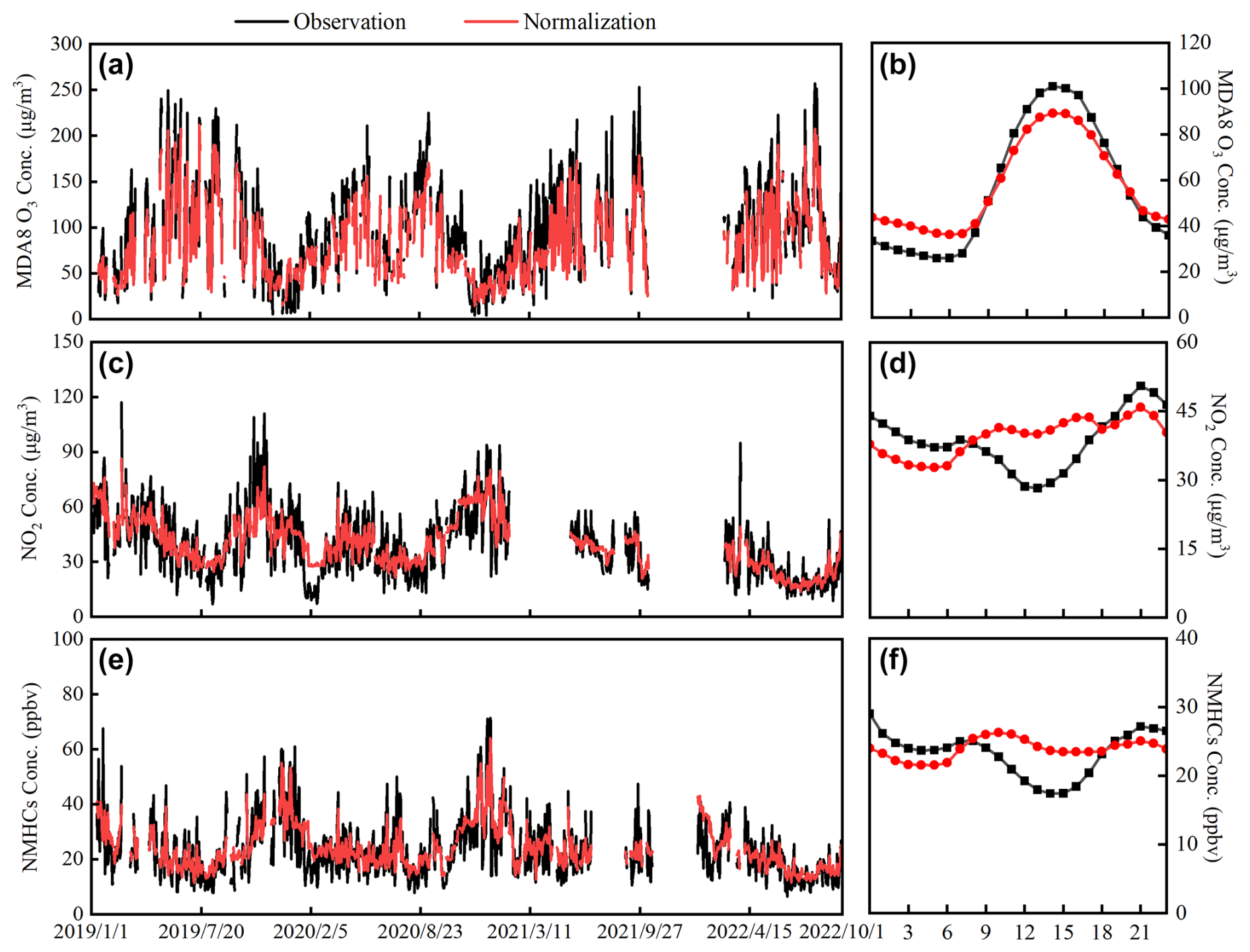
Figure 1 Long-term trends of daily average concentrations of air pollutants (a, c, e) and mean diurnal variations of air pollutant concentrations (b, d, f) based on observation and meteorological normalization from 2019 to 2022.

From the diurnal variation in NO₂ and NMHC concentrations, it is shown that the observed concentrations were lower during the day and higher at night, which was contrary to the daily trends of WS and BLH (Fig. S1). Stable WS and low BLH at night were not conducive to the diffusion of air pollutants, resulting in the accumulation of pollutant concentrations, while the situation was opposite during the day (Song et al., 2018). After the dispersion effect was removed, the precursor concentrations decreased at night and increased significantly during the day. The diurnal variation in the MDA8 O₃ concentration showed a typical single-peak structure before and after meteorological normalization. Different from the change in the concentrations of precursors, the MDA8 O₃ concentration increased at night and decreased during the day after meteorological normalization. At night, the titration reaction of NO_x and the horizontal transport reduced the O₃ concentration (Li et al., 2022). The NO_x concentration decreased after meteorological normalization, and the weakening of titration resulted in the increase in O₃ concentration at night. In addition, the decrease in horizontal transport at night also resulted in the increase in O₃ concentration after normalization. During the day, the destruction of the stable boundary layer strengthened the vertical mixing effect of the atmosphere, so that the O₃ in the upper atmosphere mixed with the O₃ generated near the surface, increasing the O₃ concentration (Lei et al., 2023). When the effect of transport was removed, the daytime MDA8 O₃ concentration decreased. It can be seen from the diurnal variations that meteorological factors directly affected the concentrations of precursors through dispersion. Meteorological factors not only directly affected the O₃ concentration through horizontal and vertical transport but also indirectly changed O₃ concentration by influencing precursor concentration and titration reaction.

Figure 2 The importance of each feature to O₃, NO₂, and NMHCs in the RF model.

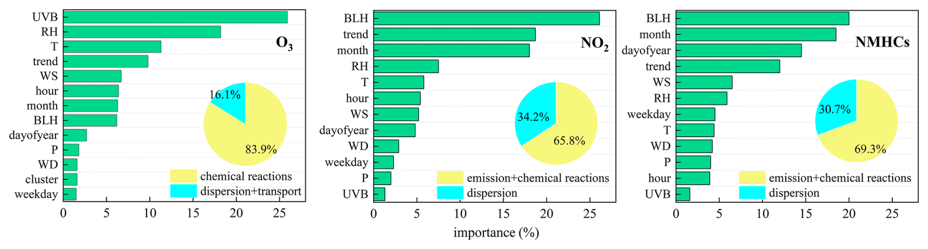
Figure 2 showed the importance of the different features in the RF model. The time variables can represent anthropogenic emissions to some extent. Time variables were closely related to the periodic changes in human activities. For example, weekdays versus weekends and peak versus non-peak hours corresponded to different levels of anthropogenic emissions. Anthropogenic emissions influenced the seasonal variations of atmospheric pollutants, as seen in winter heating effects. Previous studies also used time variables to represent anthropogenic emissions (Dai et al., 2023a, b; Song et al., 2023; Vu et al., 2019). The chemical reaction of O₃ formation was affected by meteorological factors such as UVB, T, and RH. Local dispersion of O₃ and its precursors was mainly affected by WS, WD and BLH, and long-distance transport of O₃ was characterized by the cluster. The importance of local chemical reactions to O₃ was 83.9 %. UVB, influencing photochemical reactions, emerged as the most crucial factor for O₃ concentration, with an importance of 25.9 %. This is consistent with the findings by Weng et al. (2022) in the same region. Additionally, the importance of RH and T to O₃ was also evident, with the importance of 18.2 % and 11.3 % respectively. Higher relative humidity was usually associated with a higher cloud cover, and relative humidity was generally negatively correlated with O₃ (Liu et al., 2023).

High temperatures increased the rate of most chemical reactions in the atmosphere, especially photochemical reactions that lead to O₃ formation (Li et al., 2020). In addition, elevated temperature enhanced the emission of biogenic VOCs (Lu et al., 2019). Hence, some O₃ pollution events were associated with high temperature (Dang et al., 2021). Ding et al. (2023) found that temperature was the dominant factor affecting O₃ concentration in Tianjin. Wind and BLH also played significant roles in O₃ concentration (16.1 %), mainly through vertical diffusion, vertical convection, and horizontal convection (Li et al., 2012).

Different from O₃, BLH exerted the most significant impact on NO₂ and NMHC variation, with importance values of 26.1 % and 20 %, respectively. Turbulent mixing in the active boundary layer facilitated the dispersion of air pollutants, whereas the stable boundary layer attenuated vertical diffusion, thereby intensifying the accumulation of air pollutants near the ground (Huang et al., 2020). The importance of dispersion to NO₂ and NMHCs was 34.2 % and 30.7, respectively. Consequently, unfavorable meteorological dispersion conditions can result in the accumulation of precursors, causing O₃ pollution even in scenarios with low emissions. Temporal variables representing emissions, such as month and day of year, also occupied important positions. The importance of month to NO₂ and NMHCs exceeded 18 %, which represented the significant influences of seasonal anthropogenic emissions on the concentrations of precursors. The importance of local emission, production, and consumption to NO₂ and NMHCs was 65.8 % and 69.3 %, respectively (Fig. 2).

3.1.2 Comparison between pollution and non-pollution periods

O₃ pollution occurs frequently between May and September each year. In order to evaluate the influences of meteorological conditions on the concentrations of O₃ and its precursors, the relative change in air pollutant concentrations caused by meteorological factors during O₃ pollution and non-pollution periods in the warm season (From May to September) from 2019 to 2022 was analyzed (Fig. 3). In the non-pollution periods, the negative effect of dispersion on the concentrations of NO₂ and NMHCs was apparent, with average relative changes ranging from −9.3 % to −27.98 % for NO₂ and −10.5 % to −22.8 % for NMHCs. Dispersion and transport have less influence on the MDA8 O₃ concentrations, with the average relative change ranging from −0.1 % to 8.1 %. During the pollution periods, the positive effects of dispersion and transport on O₃ became evident (from 12.9 % to 24.0 %). Simultaneously, the negative effect of dispersion on the concentrations of precursors decreased and even transformed into a positive effect. In 2021 in particular, dispersion had a significant positive effect on NO₂ and NMHCs, with an average relative change of 7.8 % and 11.8 %, respectively. O₃ concentration was affected by the long-distance transport as well as the deterioration of diffusion conditions in the pollution periods. Therefore, the influence of meteorological factors on O₃ was more obvious than that of its precursors during pollution periods in the warm season.

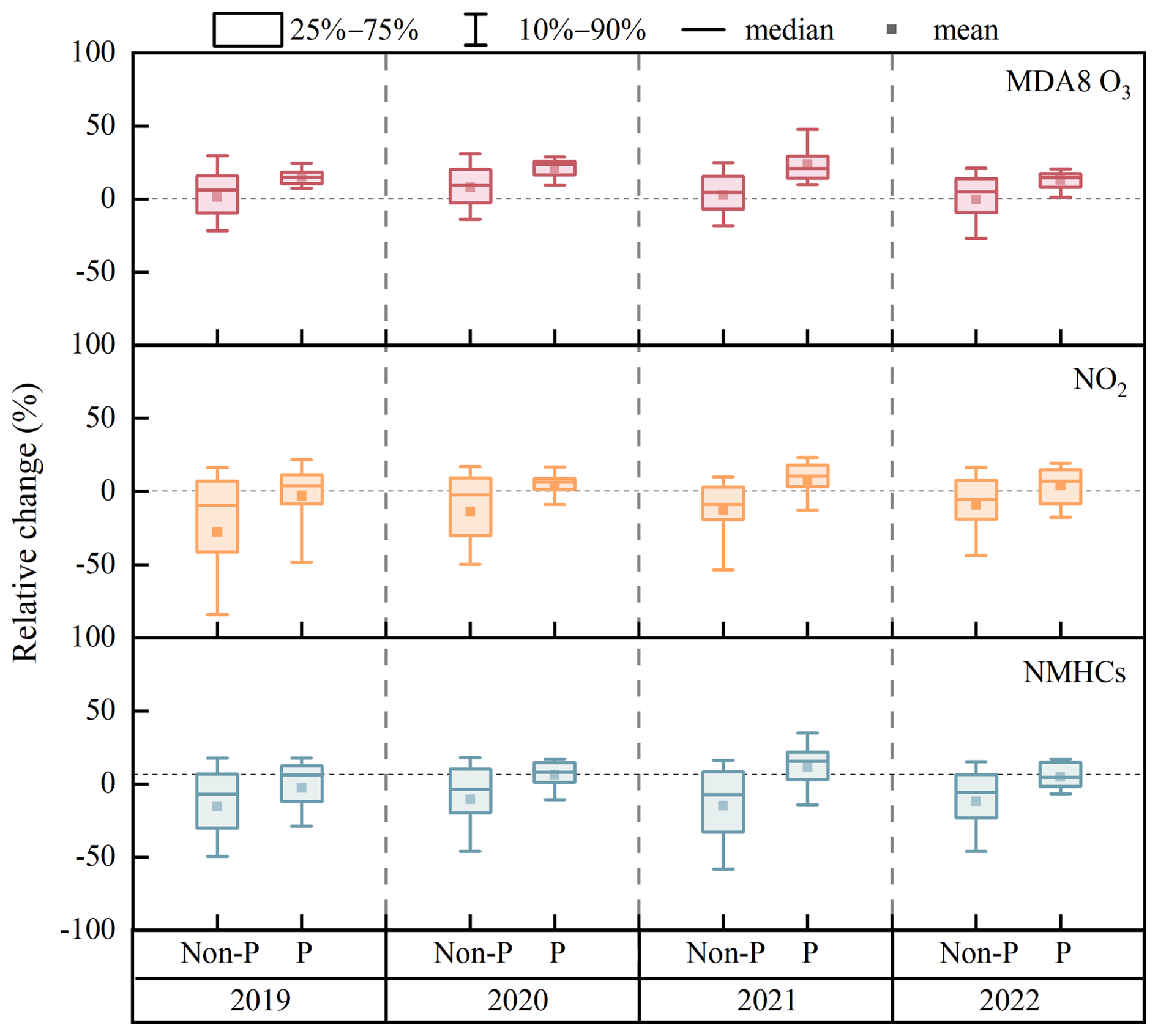
Figure 3 Relative change caused by meteorological factors during O₃ pollution (P) and non-pollution (Non-P) periods in the warm season from 2019 to 2022. Relative change = the observed concentrations − the meteorologically normalized concentrations / the observed concentrations.​​​​​​​

3.1.3 Variations during short-term pollution events

In order to explore the effects of meteorological dispersion and transport on O₃ concentration in the short term, we selected two typical pollution periods from 2019 to 2022 (Fig. 4). During Period 1 (31 August to 13 September in 2020), the average MDA8 O₃ in Hangzhou was 193 µg m⁻³ in the pollution period, exceeding the national air quality standard (> 160 µg m⁻³; GB 3095-2012, MEE, 2018​​​​​​​). At the same time, other cities in the YRD regions such as Shanghai, Nanjing, Wuxi, Changzhou, Suzhou, and Jiaxing also experienced O₃ pollution (Fig. S2). Period 1 represented a large-scale regional pollution event. During the pre-pollution period (31 August to 2 September in 2020), dispersion and transport had negative effects on MDA8 O₃. In the pollution period (3 to 10 September in 2020), the concentration of locally generated O₃ (depicted by the red line) remained below the limit, with an average concentration of 157 µg m⁻³, with only slight exceedances recorded on 6 and 9 September. Locally generated O₃ was produced in the atmosphere through photochemical reactions involving VOCs and nitrogen oxides (NO_x; Song et al., 2021). However, the actual observed O₃ concentration was much higher than the standard, and the O₃ concentration was about 200 µg m⁻³ from 6 to 10 September. The positive contribution of dispersion and transport was significant (depicted by the red area) in the pollution periods, resulting in an 18.7 % increase in the MDA8 O₃ concentration. During the post-pollution period, contributions of dispersion and transport decreased significantly.

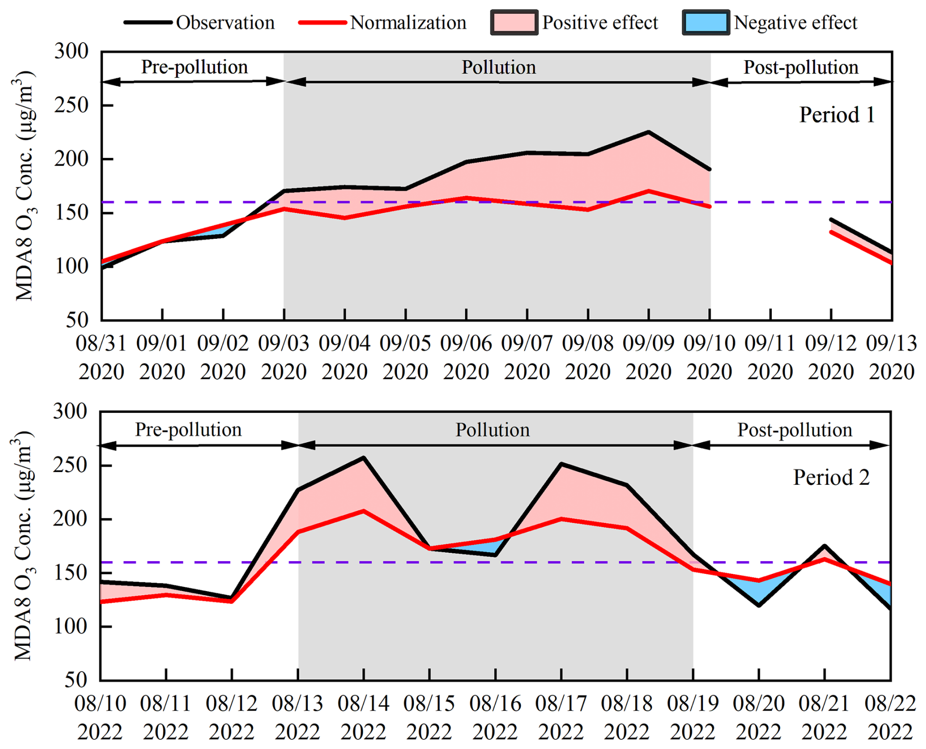
Figure 4 The MDA8 O₃ concentration based on observation and meteorological normalization and the contributions of dispersion and transport to the MDA8 O₃ during pre-pollution, pollution, and post-pollution periods in Period 1 and Period 2 (red: positive contribution, blue: negative contribution).

In Period 2 (10 to 22 August in 2022), the average MDA8 O₃ concentration in Hangzhou was as high as 211 µg m⁻³ during the pollution period, while the concentration of MDA8 O₃ in most surrounding cities was less than 160 µg m⁻³. Thus the O₃ pollution in Period 2 was influenced by both local formation and transport. During the pollution period (13 to 19 August in 2022), locally generated O₃ basically exceeded the standard, and the MDA8 O₃ concentration was greater than 180 µg m⁻³ on most days, with an average concentration of 185 µg m⁻³. On 16 August, the meteorological negative contribution (−14.4 %) appeared, exerting dilution effects on the O₃ concentration, but the MDA8 O₃ on that day still exceeded 160 µg m⁻³, indicating intense local O₃ production. The positive contributions of dispersion and transport to O₃ were significant during the pollution periods; the contributions ranged from 8.5 % to 20.4 %. For precursors, the concentration of NMHCs increased between 17 and 19 August (Fig. S3). The positive contribution of dispersion to NO₂ and NMHCs ranged from 4.4 % to 13.7 % and from 0.6 % to 8.5 % during pollution. During the post-pollution period (20 to 22 August in 2022), the contributions of dispersion and transport turned negative, indicating that meteorological diffusion conditions favored the elimination of O₃ pollution.

3.2 VOC–NO_x–O₃ sensitivity

Unfavorable meteorological conditions can cause the accumulation of O₃, making it essential to have a clear understanding of local O₃ formation pathways for effective control of O₃ pollution. The relationship between O₃ and NO₂ under long-term trends was analyzed based on the observed (left) and meteorologically normalized (right) data (Fig. 5). The dotted red line shows the turning point of the relationship between O₃ and NO₂ concentrations. The blue triangle represented the average value of the MDA8 O₃ during the warm season each year. On the left side of the dotted red line, O₃ concentration elevated with the increase in NO₂ concentration. At this point, controlling the emission of NO₂ was conducive to limiting the formation of O₃, suggesting that the sensitivity of O₃ formation was limited by NO_x. On the right side of the dotted red line, O₃ concentration decreased with the increase in NO₂ concentration. At this point, the inhibition effect of NO_x emission reduction on O₃ formation was not significant, and it is necessary to control the emission of VOCs, indicating that the sensitivity of O₃ formation was limited by VOCs (Kong et al., 2024). After meteorological normalization, the NO₂ concentration in the turning point increased from 9 to 19 µg m⁻³, suggesting that when NO₂ concentration was at a higher level, O₃ concentration decreased with the increase in NO₂ concentration. In other words, a higher NO₂ value at the turning point suggested a greater likelihood that the actual NO_x concentration was below that value, indicating a higher probability of being in a NO_x-limited regime. In addition, based on average results in warm season each year, the sensitivity of O₃ formation before and after meteorological normalization was also shown in Fig. 5. Whether based on observed or meteorologically normalized data, the O₃ formation from 2019 to 2021 was located in the VOC-limited regime, while O₃ production entered the transition regime between VOC- and NO_x-limited regimes in 2022. The transition regime referred to the region near the turning point, where O₃ formation was sensitive to changes in both VOCs and NO_x.

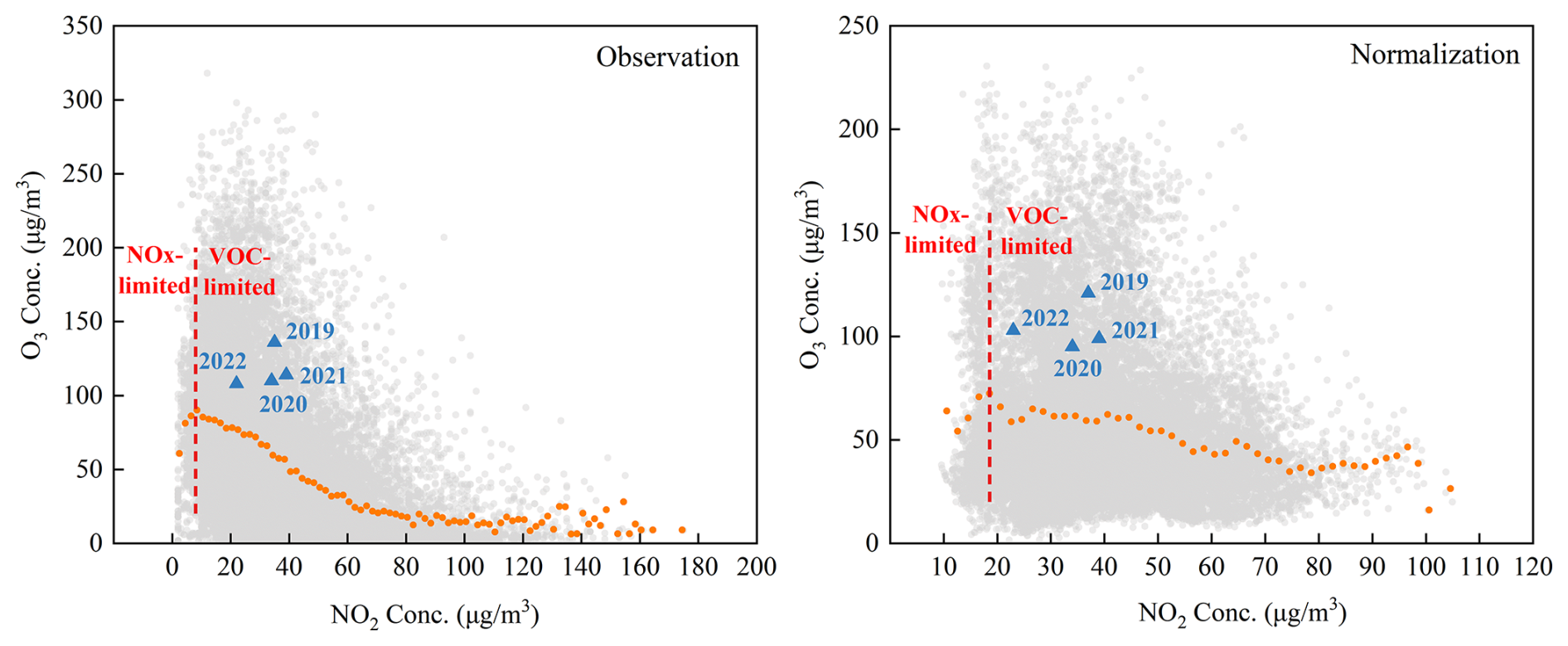
Figure 5 The changes in O₃ concentration and NO₂ concentration from 2019 to 2022. The light-gray circles represent the hourly O₃ concentration. The orange circles represent the average value of O₃ concentration in each interval (2 µg m⁻³) of NO₂. The blue triangle represents the average value of the MDA8 O₃ during the warm season each year.

The OBM was used to analyze the sensitivity of O₃ formation. The OBM is zero-dimensional, meaning it excludes the processes of atmospheric transport and dispersion. Therefore, it is reasonable to remove the influences of transport and dispersion when using the OBM. The VOC–NO_x–O₃ sensitivity and the net ozone production rate (P(O₃)) exhibited significant differences before and after meteorological normalization in the short-term pollution events (Fig. 6). The O₃ concentration in Period 2 was affected by both transport and local formation. The concentration of local precursors increased after removing the effect of dispersion, resulting in the change in the sensitivity of O₃ formation. Based on the observation results, the O₃ formation in pollution was located in the strict NO_x-limited regime. After meteorological normalization, O₃ formation shifted towards the transition regime between VOC- and NO_x-limited regimes. The limitation of O₃ formation by NO_x concentration was weakened. After removing the influence of dispersion and transport on O₃ concentrations, the value of P(O₃) increased, indicating that the P(O₃) calculated based on observation was likely underestimated. Therefore, when the OBM was used to analyze the VOC–NO_x–O₃ sensitivity, removing the influences of dispersion and transport was beneficial to accurately identify the limited regime of O₃ formation.

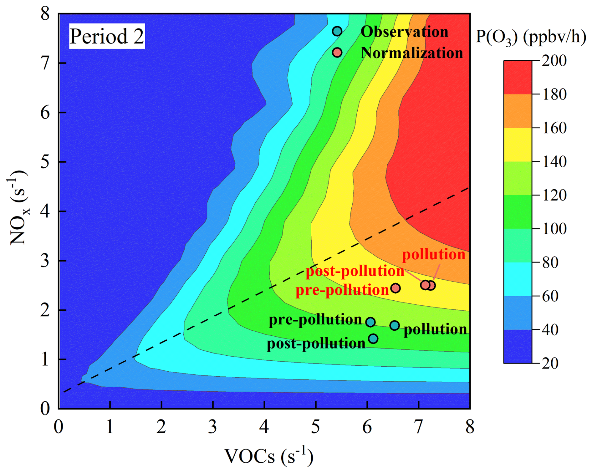
Figure 6 The O₃ isopleth diagram versus NO_x and anthropogenic VOCs using the EKMA. The circles represent the average concentrations of NO_x and VOC during pre-pollution, pollution, and post-pollution periods in Period 2.

3.3 VOC source apportionment

The PMF method was further used for VOC source analysis. The optimal solution was selected by examining the interpretability of factors and the distribution of scale residuals. Based on observed and meteorologically normalized concentrations, seven possible emission sources of VOC from May to September in 2022 were extracted using the US EPA PMF v5.0. The possible emission sources of VOC included combustion, industrial source, vehicle exhaust, fuel evaporation, secondary and aging source, biogenic source, and solvent use. The differences in the source profiles resolved from the observed and normalized concentrations are illustrated in Fig. S5.

The combustion source was characterized by high concentrations of ethane, propane, and acetylene. Low carbon alkanes and alkenes were likely to be the products of incomplete combustion (Wang et al., 2015). Acetylene was a typical tracer of combustion. Toluene and some halohydrocarbons, such as chloromethane, were also released from combustion (Liu et al., 2008). Additionally, the proportion of acetonitrile was also high, which was an important product of biomass combustion (de Gouw et al., 2003). Biomass combustion emission was relatively intense in the YRD. The industrial source was characterized by halohydrocarbons (Sun et al., 2016), and 1,2-dichloroethane accounted for nearly 80 % of this factor in both PMF results. Vehicle exhaust was featured by high concentrations of ethane, propane, isobutane, n-butane, isopentane, ethylene, and toluene(Cai et al., 2010; Liu et al., 2008). Fuel evaporation was characterized by the high concentration and proportion of isopentane, isobutane, n-butane, and n-pentane, while the concentration of acetylene was minimal in this factor. The secondary and aging source was characterized by halohydrocarbons and oxygenated VOCs (OVOCs). Methacrolein (MACR) and methyl vinyl ketone (MVK) were products of the oxidation of isoprene (Mo et al., 2018). OVOCs and halohydrocarbons have long lifetimes in the atmosphere and can serve as important tracers for aging sources (Yang et al., 2021b). The biogenic source was featured by highest concentration of isoprene, primarily emitted by plants (Gong et al., 2018). Additionally, the oxidation products of isoprene (MACR and MVK) also contributed to this factor. The solvent source was characterized by high concentrations of aromatics. Toluene, ethylbenzene, m-xylene, and o-xylene are commonly used as materials in solvents (Song et al., 2021).

After smoothing out the effect of dispersion, the absolute contribution of emission sources to VOCs changed. The mean absolute contribution of vehicle exhaust to VOCs increased most significantly, from 3.97 to 6.72 ppbv during the non-pollution periods and from 6.84 to 9.76 ppbv during the pollution periods. The mean absolute contribution of combustion decreased by 1.55 and 2.09 to 2.86 and 5.85 ppbv during the non-pollution and pollution periods, respectively. Dispersion caused overestimation of the contribution of combustion to VOCs, which indicates that the reduction in VOC concentration by abatement measures can be offset by the effect of dispersion. Therefore, the impact of dispersion should be taken into account when evaluating the effectiveness of emission reduction measures on VOC emission sources. The normalized contributions of solvent use and industrial source in the pollution were comparable, with an average absolute contribution of 2.78 and 2.57 ppbv. In comparison to the results based on the observations, the absolute contribution of fuel evaporation decreased from 1.94 to 1.33 ppbv after meteorological normalization during the pollution periods. After meteorological normalization, the contributions of biogenic source and secondary and aging source to VOCs during the pollution period were relatively low, with absolute contributions of 0.54 ppbv.

Figure 8 showed the proportion of VOC sources before and after meteorological normalization during the non-pollution periods and pollution periods. The pie charts for normalized source contributions illustrate the relative contribution of each source to the total VOC concentration after removing the effects of dispersion. According to the results of the observations, combustion and vehicle exhaust were the largest contributors to VOCs, accounting for 27.1 % and 24.3 % in the non-pollution periods. And the proportion of combustion and vehicle exhaust increased to 33.7 % and 29 % in the pollution periods. During the pollution periods, the proportion of solvent use and fuel evaporation also increased, accounting for 15.9 % and 8.2 %, respectively. After the normalization of dispersion, vehicle exhaust became the predominant emission source of VOCs (37 % in the non-pollution periods and 41.8 % in the pollution periods), much higher than the proportion of other emission sources. According to the motor vehicle data released by the Zhejiang Public Security Department in 2022, the number of motor vehicles reached 23.29 million. During the non-pollution periods, the contributions of solvent use, industrial source, and combustion were comparable, accounting for the proportions ranging from 15.6 % to 16.2 %. Compared to the non-pollution periods, the influence of combustion on VOCs increased (25.1 %), while the proportions of industrial source and solvent use decreased during the pollution periods (11 % and 11.9 %). Straw burning occurs frequently in Zhejiang Province. According to the remote sensing monitoring of straw burning announced by the Ecological Environment Monitoring Center of Zhejiang Province, a total of 135 straw-burning points in the province were monitored by satellite remote sensing from January to October 2022. The proportion of industrial emission and solvent use decreased during the pollution periods, and the VOC concentrations from these two sources also declined (Fig. 7), indicating that the implementation of shutdown or off-peak production measures at the time of pollution warning was effective.

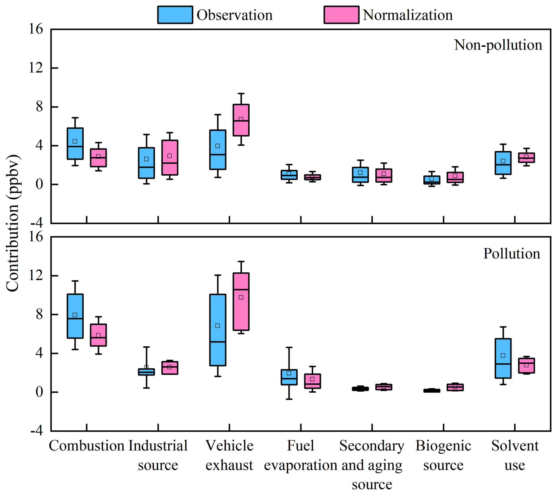
Figure 7 The absolute contributions of emission sources to VOCs based on observation and meteorological normalization during the non-pollution periods and pollution periods in the warm season in 2022.

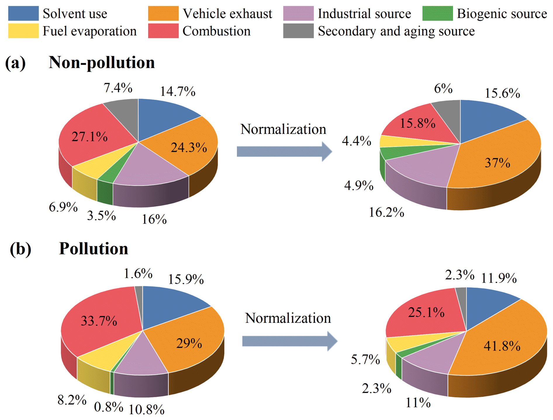
Figure 8 Comparison of VOC source proportions before and after meteorological normalization during the non-pollution periods and pollution periods in the warm season in 2022.

The O₃ formation potential (OFP) is used to assess VOC photochemical activity (Carter, 2010), and it can be calculated using Eq. (2):

$$\begin{array}{}\text{(2)}& {\mathrm{OFP}}_i={\mathrm{MIR}}_i\times \left[{\mathrm{VOC}}_i\right],\end{array}$$

where MIR_i represents the maximum incremental reactivity for VOC species i, and [VOC]_i represents the concentration of VOC species i (µg m⁻³). MIR values for each VOC species were taken from the updated Carter research results (https://intra.engr.ucr.edu/~carter/SAPRC/​​​​​​​, last access:​​​​​​​ 1 February 2025). The contributions of emission sources to OFP were further analyzed and are shown in Fig. 9. Based on the results of the observations, the emission sources that contribute the most to OFP were solvent use (67.79 µg m⁻³), vehicle exhaust (33.16 µg m⁻³), and combustion (29.16 µg m⁻³) during the pollution periods in the warm season in 2022. After removing the effect of dispersion, the contribution of vehicle exhaust to OPF increased to 47.25 µg m⁻³, while the contribution of solvent use and combustion to OFP decreased to 54.77 and 22.58 µg m⁻³, respectively. The actual contributions of combustion and solvent use to O₃ formation were larger under the dispersion effect. Thus, it was necessary to consider the cumulative effect of dispersion and enhance emission reduction measures for specific emission sources. For Period 2 mentioned in Sect. 3.1.3, we also found that the contributions of VOC emission sources changed after meteorological normalization (Figs. S6 and S7). After removing the dispersion effect, the contributions of solvent use and vehicle exhaust to OFP increased during the pollution periods, while the contribution of combustion and secondary and aging source decreased. From 17 to 19 August, the normalized contribution of solvent source to OFP was significant, with an average OFP of 105.81 µg m⁻³, indicating that the emission of solvent source was enhanced on these days. The dispersion effect of meteorological conditions on precursors can conceal the real information of emission sources and misjudge the formation process of O₃.

Figure 9 The contributions of emission sources to OFP based on observation and meteorological normalization during the pollution periods in the warm season in 2022.

4 Conclusion

In this paper, a RF model was established based on the hourly data of 4 years of continuous observation, and some meteorological effects on the concentration time series of air pollutants were “removed”. Transport and dispersion effects were removed for O₃, and the dispersion effect was removed for its precursors. In the process of building the RF model, UVB, RH, and T were found to be the most important factors affecting O₃ concentration, with the importance of 25.9 %, 18.2 %, and 11.3 %, respectively. Local influences, including precursor emissions and secondary photochemical reactions, occupied 83.9 % of the importance to O₃ concentration. To understand the mechanisms of local O₃ formation, the meteorological effects were analyzed in long-term trends, pollution and non-pollution periods in the warm season, as well as short-term pollution events. After decoupling meteorological effects, the concentration trends of O₃ were consistent with those observed in the long term, indicating that O₃ concentration was mainly driven by precursor emissions and local chemical reactions. During the pollution periods in the warm season from 2019 to 2022, the positive contributions of dispersion and transport to the MDA8 O₃ ranged from 12.9 % to 24.0 %. The effects of dispersion and transport were further analyzed for different types of O₃ pollution events. For transmission-type O₃ pollution (Period 1), dispersion and transport contributed 18.7 % to the MDA8 O₃ concentration, increasing the mean MDA8 O₃ concentration from 157 to 193 µg m⁻³. For local and transmission-type O₃ pollution (Period 2), the average locally generated MDA8 O₃ concentration was 185 µg m⁻³. Under the influences of dispersion and transport, the average MDA8 O₃ concentration increased to 211 µg m⁻³, and the positive contributions of dispersion and transport ranged from 8.5 % to 20.4 %. BLH, as a parameter of dispersion, was of the highest importance for NO₂ and NMHCs, accounting for 34.2 % to NO₂ and 30.7 % to NMHCs. Therefore, precursor concentrations were accumulated even in the case of low emissions when the dispersion condition was poor, promoting the photochemical production of O₃. This also corresponds to the fact that even with the implementation of precursor emission reduction policies, O₃ concentrations in urban areas remain persistently high.

By decoupling the influences of meteorological conditions, it was observed that the sensitivity of local O₃ formation and the apportionment of VOC emission sources have changed. From the EKMA of short-term pollution events, the sensitivity of O₃ formation in Period 2 shifted towards the transition regime between VOC- and NO_x-limited regimes after meteorological normalization. Based on the PMF model, the changes in VOC emission sources after removing the dispersion effect during the warm season in 2022 were further analyzed. After removing the effect of dispersion, the absolute contribution of vehicle exhaust to VOCs during the pollution was 9.76 ppbv, accounting for 41.8 %, and the contribution of vehicle exhaust to OFP was 47.25 µg m⁻³. The contribution of vehicle exhaust to VOCs was underestimated due the dispersion effect. After meteorological normalization, combustion remained an important source of VOCs, contributing 25.1 % during the pollution period, which was overestimated by 8.6 %. The normalized contribution of solvent use to VOCs decreased to 11.9 %, but it is undeniable that solvent use was still a crucial contributor to OFP, contributing 54.77 µg m⁻³. Neglecting the influences of meteorology can lead to a deviation in emission reduction priorities, and the effectiveness of emission reduction may be masked by unfavorable meteorological conditions. The conclusion of this research suggested that meteorological fluctuations can interfere with the results of the OBM and PMF. Decoupling meteorological effects before using traditional models was beneficial for deepening the understanding of local O₃ formation and improving the rationality of precursor emission reduction measures.