The frosty frontier: redefining the mid-latitude tropopause using the relative humidity over ice

The tropopause represents a central feature of the atmospheric vertical structure, marking the transition between the troposphere and stratosphere. While common definitions rely on quantities conserved under adiabatic changes, diabatic effects, resulting from radiation, cloud processes or turbulence are also decisive for the tropopause structure. Therefore, we propose a new definition based on the vertical gradient of the relative humidity with respect to ice (RHi). RHi is the key variable for ice cloud formation and incorporates both diabatic and adiabatic processes. Based on high-resolution radiosonde data, we can show that our RHi-GT-based definition is generally consistent with, and often provides a clearer characterization than the thermal tropopause. This is not only evident in individual vertical profiles, but also when looking at statistics of many profiles with a tropopause-relative height axis. Last but not least, the robust and simple calculation of our definition makes it an ideal tool for studies involving the tropopause.

1 Introduction

The Earth's atmosphere extends from the ground to several hundred kilometers above the surface. It is characterized by several layers that are distinguished by thermal, chemical, and dynamic properties. The transition from one layer to another is usually abrupt and is noticeable through strong gradients in the respective variables. The active weather layer that determines our lives is the troposphere and extends from the ground to an altitude of about 8 to 12 km in the mid-latitudes, depending on the seasons and current weather situation. In extreme cases, there are also strong upward and downward deviations from this altitude range. The layer above is the stratosphere, which is characterized by very dry conditions and a general increase in temperature with altitude. The troposphere and stratosphere are separated by the tropopause and the transfer between these two spheres, the so-called stratosphere-troposphere exchange (STE), affects key properties of the different layers (Gettelman et al., 2011). For instance, transport of water vapor from the troposphere into the stratosphere affects radiative properties of the stratosphere (Krebsbach et al., 2006), while the transport in the opposite direction can enhance the tropospheric ozone concentration (Stevenson et al., 2006). Thus, the determination of the tropopause is of high relevance for our understanding of the upper troposphere/lower stratosphere (UTLS) region. However, it should be noted that there are still uncertainties in the description of exchange processes in large-scale models (Charlesworth et al., 2023; Hoffmann and Spang, 2022).

There are many different ways to define the tropopause, mostly based on threshold values or gradient changes of different variables such as (potential) temperature, potential vorticity, or even concentrations of chemical substances (e.g. ozone). One of the most widely used definitions is the so-called thermal tropopause (TTP), as defined by the WMO (WMO, 1957), which has a somewhat cumbersome wording:

The first tropopause is defined as the lowest level at which the lapse rate decreases to 2 K per kilometer or less, provided also the average lapse rate between this level and all higher levels within 2 kilometers does not exceed 2 K (WMO, 1957).

This definition is frequently used for studies of the extratropical UTLS and is often referred to as the lapse rate tropopause. In the following, we refer to this tropopause definition as a thermal tropopause.

Instead of the physical temperature, sometimes the potential temperature as a quantity conserved under adiabatic processes is used for the determination of the tropopause. For instance, the vertical gradient of potential temperature is utilized for the determination of the tropopause (Mullendore et al., 2005; Kohma and Sato, 2019). An advantage of these temperature-based tropopause definitions is its ease of use, as a single temperature profile, e.g. from a radio sonde ascent or extracted from model data, is sufficient to determine the tropopause height (Reichler et al., 2003). While these definitions were originally formulated with synoptic-scale flows in mind, assuming pronounced vertical gradients, they explicitly allow for the identification of multiple tropopauses within a single profile, for example in regions influenced by the jet stream (Pan et al., 2004; Randel et al., 2007; Castanheira and Gimeno, 2011). It should be noted, however, that very high vertical resolution can pose challenges for this approach, as discussed by Tinney et al. (2022).

A determination of the tropopause based on dynamic properties goes back to Reed (1955), who used the potential vorticity, a quantity conserved under adiabatic processes, as the basis for determining the tropopause. This dynamic tropopause is the interface between the troposphere based on the potential vorticity (PV) with low values in the troposphere and high values in the stratosphere. For dynamic processes in the mid-latitude tropopause region different PVU values are used in the literature, which are generally between 2 and 3.5 PVU (Kunz et al., 2011; Hoerling et al., 1991), leading to a kind of indeterminacy in the use of this definition. An advancement based on this is the PV gradient method, which avoids picking a particular value of PV (Kunz et al., 2011; Turhal et al., 2024).

Finally, it is also possible to define a tropopause on the basis of concentrations of individual chemical substances. In Bethan et al. (1996), for example, an ozone (O₃) concentration of 100 ppb is used to define the ozonopause, which is generally close to the thermal tropopause. In a recent publication by Bauchinger et al. (2025) the authors used several tropopause definitions, including one based on nitrous oxide (N₂O), where the tropopause was determined using a statistical baseline approach. Tracer-tracer correlations are also sometimes used for the determination of a tropopause (Pan et al., 2004).

The reader is referred to Köhler et al. (2024), Bauchinger et al. (2025), and Hoinka (1997) for detailed reviews of different tropopause definitions, including some, such as the cold-point tropopause, that are not applied in the present study because they are primarily relevant for tropical regions.

From a more physical perspective, the tropopause structure is determined by the interplay of various different processes on many scales, i.e. adiabatic and diabatic contributions. In the UTLS, synoptic-scale vertical motions are relatively weak, but larger-scale mean circulations such as the Brewer–Dobson circulation play a central role: they are characterized by rising air in the tropics, poleward transport in the stratosphere, and descending motion in the mid- and high latitudes (Butchart, 2014; Seviour et al., 2012). This results in adiabatic cooling in the tropical ascent region and adiabatic warming at mid- to high-latitudes.

On the other hand, diabatic processes play a role. Water vapor (and also solid water particles, i.e. ice crystals) is absorbing and re-emitting infrared radiation as an almost ideal black body, leading to a local cooling on top of moist layers situated close to the tropopause. At this level, strong vertical gradients in temperature and humidity make moist layers particularly effective in modifying the local radiative balance (Fusina and Spichtinger, 2010). In addition, ice particles play an important role for the interaction with shortwave radiation, further contributing to the radiative impact of tropopause-near moist layers. Radiative heating rate estimates (Fusina and Spichtinger, 2010) suggest characteristic time scales of several hours 𝒪(10 h), which are relevant compared to the lifetimes of upper-tropospheric moist layers (e.g. Irvine et al., 2014; Spichtinger et al., 2005). Recent results (Emig et al., 2025) also indicate that long-lived cirrus clouds can modify the tropopause structure, confirming the key role of radiation on these time scales. Finally, friction and irreversible mixing, as e.g. driven by turbulence, contribute to the change in variables as diabatic processes.

Usual definitions of the tropopause, as mentioned above, rely mostly on adiabatic processes, which can be determined by investigating e.g. the physical or even potential temperature or potential vorticity (which both are conserved under adiabatic processes by definition). Yet diabatic processes – including radiative cooling, latent heating, and small-scale mixing – also shape the tropopause structures, as exemplified by the tropopause inversion layer (TIL) (e.g., Birner et al., 2002; Randel et al., 2007; Fusina and Spichtinger, 2010; Spichtinger, 2014; Köhler et al., 2024; Kunkel et al., 2016). Relative humidity over ice (RHi) captures both adiabatic and diabatic contributions to TIL formation, motivating a tropopause definition based on RHi gradients.

Section 2 will introduce the used data as well the description of the new tropopause definition. In Sect. 3 the performance of the tropopause definition is presented for three cases as well as for a statistical analysis over 10 year. The influence of the threshold values for determining the RHi-GT is then analysed in Sect. 4. Finally, some conclusions are drawn in the summary section.

2 Data and Methods

Here we describe the used data and introduce the newly derived tropopause definition based on the vertical gradient of the relative humidity over ice.

2.1 Radiosonde data

In this study, we use high-resolution radiosonde data from the German Weather Service (DWD) from Meiningen in Central Germany (50.56173° N, 10.37693° E, altitude of 450 m above sea level), where operational radiosonde ascents are carried out twice a day (00:00 and 12:00 UTC). We use the data from 7565 radiosonde ascents between 1 January 2015 to 31 December 2024 (i.e. full 10 years of data). Until 6 September 2017 the measurements were conducted using the Vaisala RS92-SGP sonde. After that the Vaisala RS41-SGP sondes were in operation. Both types are of similar quality and were used before for investigations of the tropopause region (Köhler et al., 2024). For the RS92-SGP, the temperature sensor has a response time <2.5 s with an uncertainty of 0.5 °C, while the humidity sensor responds within 0.5–20 s with an uncertainty of 5 % RH. In the RS41-SGP, the temperature sensor is faster (≈0.5 s) and more accurate (0.2 °C), and the humidity sensor responds within 0.3–10 s with an uncertainty of 5 % RH. The RS92-SGP measurement uncertainties are specified by the manufacturer (https://www.bodc.ac.uk/data/documents/nodb/pdf/RS92SGP-Datasheet-B210358EN-F-LOW.pdf, last access: 24 September 2025). The RS41-SGP measurement uncertainties are specified by the manufacturer (https://docs.vaisala.com/v/u/B211444EN-J/en-US, last access: 24 September 2025).

The data has been converted to a regular vertical grid with a resolution of 50 m. All further examinations were carried out on this grid. The relative humidity over ice is calculated by following equation

$$\begin{array}{}\text{(1)}& \mathrm{RHi}=\mathrm{RH}\cdot {\displaystyle \frac{p_{\mathrm{s},\mathrm{liq}}\left(T\right)}{p_{\mathrm{s},\mathrm{ice}}\left(T\right)}}\end{array}$$

where RH is the relative humidity with respect to liquid (directly measured by the radiosonde), p_s,liq(T) is the saturation vapor pressure with respect to liquid water calculated using the Magnus formula (Alduchov and Eskridge, 1996), and p_s,ice(T) is the saturation vapor pressure with respect to ice obtained by the formula from Murphy and Koop (2005). Radiosondes typically ascend with a vertical velocity of about 5 m s⁻¹ (≈ 300 m min⁻¹), such that they reach 16 km altitude within roughly 45–55 min (World Meteorological Organization, 2025). The time indicated marks the launch of the radiosonde.

2.2 Tropopause definition

Two different tropopause definitions are used in this study. The previously widely used WMO definition based on absolute temperature (thermal or lapse rate tropopause) and a newly developed definition based on the gradient of relative humidity with respect to ice. The latter is described first.

2.2.1 RHi Gradient Tropopause – RHi-GT

The aim of this definition is to realize a tropopause definition based on the relative humidity over ice. As a final result, it should indicate a troposphere that is significantly more humid than the stratosphere. On the one hand, this could be achieved by applying a simple threshold, for example setting RHi to 10 %. However, it is very difficult to measure (absolute) humidity at very cold temperatures (implying low water vapor concentrations), such as those prevailing in the tropopause region. In order not to be dependent on error-prone absolute values, a gradient method is chosen here. The calculation of the relative humidity over ice gradient tropopause (RHi-GT) is explained in the following:

Top-down Search: The algorithm starts at the highest point of the radiosonde ascent and defines the tropopause height according to the following scheme:

1. RHi Threshold: The relative humidity with respect to ice must exceed 10 %.

2. Vertical Relative Humidity Gradient: The derivative of RHi with height ($\partial \mathrm{RHi}/\partial z$) must be smaller than −0.15 % m⁻¹. This gradient threshold is based on empirical analyses and ensures that the tropopause height is detected in regions with a strong RHi gradient.

3. Tropopause Height Assignment: As soon as both criteria are met, the corresponding height is stored as the tropopause height RHi-GT.

4. Break Criterion: To avoid unrealistically low tropopause heights, any detected height below 3000 m is discarded and no value is assigned for that profile.

In a total of 7565 radiosondes, no RHi-GT was found in 42 cases (0.56 %). Additionally, it is important to note that the choice of the threshold may differ for other geographic regions.

2.2.2 Thermal tropopause TTP

For the detection of the thermal tropopause the WMO criterion (WMO, 1957) is used, while we only search for the first tropopause. With this definition of a tropopause, it is also possible that no tropopause height is found. This is the case for 18 radiosonde ascents (0.24 %). The results of both tropopause definitions (red-dotted: thermal tropopause; blue-dashed: RHi-GT) can be seen in Figs. 1 to 3.

Note that the high resolution data of temperature raise issues in terms of determining the lapse rate; a smoothing of the profiles is applied for extracting the large scale feature of thermal profiles. For this we use the identical algorithm as in Köhler et al. (2024).

3 Results

For our investigations, we define the tropopause via the gradients of relative humidity, as described in Sect. 2, termed relative humidity over ice gradient tropopause (RHi-GT) in the following. Here we present the results of the new RHi-GT definition for the estimation of the tropopause height, based on high-resolution radiosonde data. First, three different real-life situations are shown to demonstrate the capabilities of the RHi-GT definition, also in contrast to the commonly used WMO definition. The first situation shows a good agreement with the thermal tropopause, while the other two situations show a higher and lower RHi-GT height, respectively. Furthermore, the distances between the two tropopause definitions during the 10-year observation period are shown (Fig. 4). Finally, we present the results relative to the RHi-GT and thermal tropopause, and consider mean profiles.

3.1 Comparison of tropopause definitions

To evaluate the performance of the new tropopause definition, we first examine three representative cases that are intended to cover different relative positions of the RHi-GT with respect to the thermal tropopause, namely situations where the RHi-GT is located above, approximately at, or below the thermal tropopause. The first example in Fig. 1 shows a case in which the thermal tropopause and the RHi-GT are close to each other. We see a distinct thermal tropopause with a sharp inversion at the tropopause level. The RHi-GT is likewise directly visible in the profile of the potential temperature, as a strong positive vertical gradient develops with the tropopause height. Additionally, there is a sharp drop in RHi from very high values above 100 % RHi to values below RHi≤15 %. The sharp transition is also visible in the specific humidity profile.

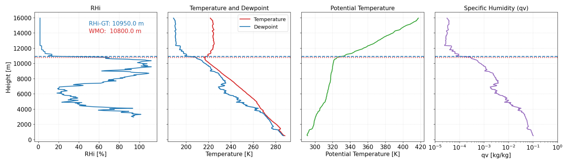
Figure 1 Vertical profile of RHi, temperature (red), dew point (blue), potential temperature and specific humidity of the radiosonde ascent from Meiningen, 2 June 2024, 12:00 UTC. RHi values are shown for temperatures below 273.15 K. The RHi-GT level (blue-dashed) and thermal tropopause level (red-dotted) are shown in every subplot.

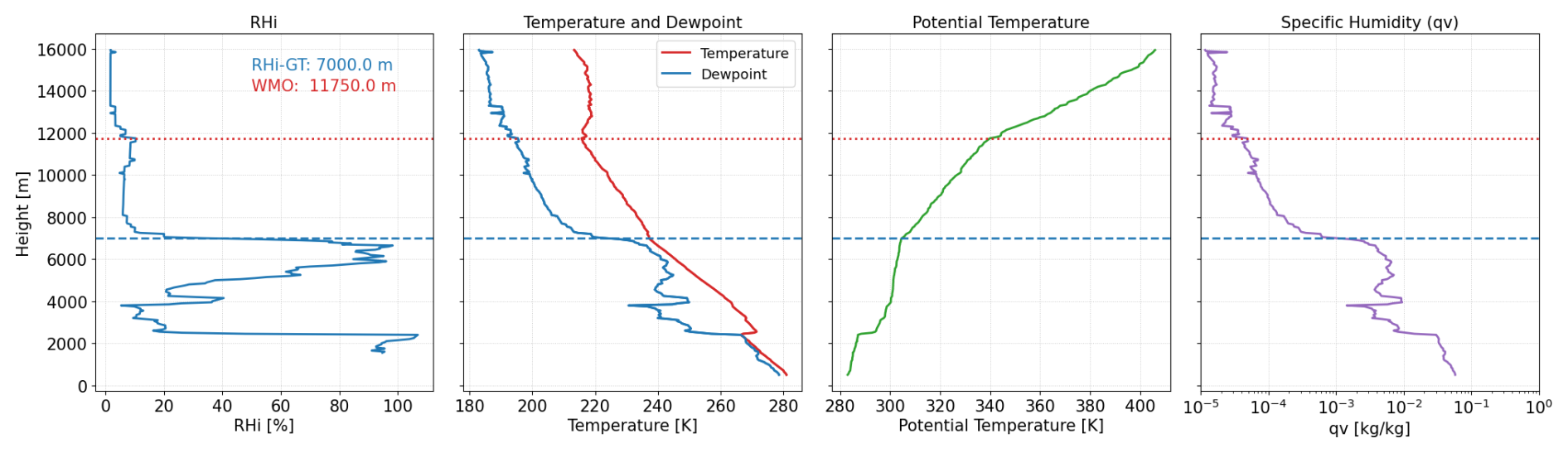
The second example displays a situation where the RHi-GT is significantly lower than the thermal tropopause. Figure 2 shows a case from 18 February 2024 where the thermal tropopause is calculated at a height of 11.75 km in contrast to the height corresponding to the RHi-GT definition of 7.0 km. In contrast to the case above (Fig. 1) the signature of the thermal tropopause is not as distinct. In the potential temperature profile a first significant increase of the vertical gradient coincides with the RHi-GT level at 7.0 km. This means the high RHi values just below the RHi-GT and an increase in stability fall together, while the absolute temperature still decreases for almost 5 km until the thermal tropopause is reached. At this point the vertical gradient of θ is increasing once more. From the RHi-GT point of view, however, we are already deep in the stratosphere, which makes sense with respect to the values of absolute humidity; we see the strong change in absolute humidity occurring at the RHi-GT level, too. In summary, this indicates a strong confinement of water vapor at the RHi-GT level, whereas the conventional thermal tropopause definition fails completely to detect this feature.

Figure 2 Same as Fig. 1, but for 18 February 2024, 00:00 UTC.

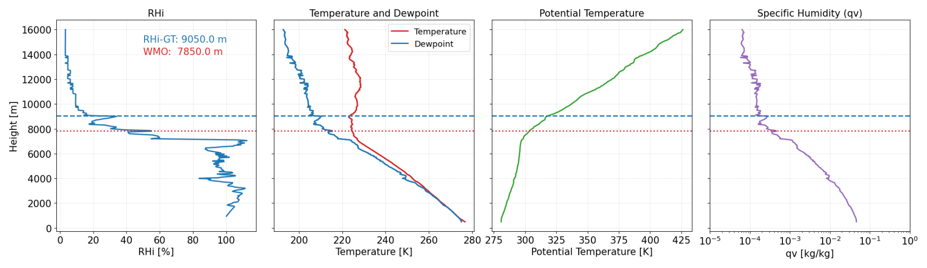
The last example in Fig. 3 exhibits a higher RHi-GT (9.1 km) compared to the thermal tropopause (7.9 km). A purely visual determination of the thermal tropopause is difficult here, as the absolute temperature changes only slightly over a deep layer. The WMO thermal tropopause therefore appears somewhat arbitrary at this point. Based on the potential temperature, the tropopause could possibly be placed even lower. However, it is noticeable that a locally strong gradient in the potential temperature is present at the height of the RHi-GT. This again shows that the RHi-GT definition is also meaningful in terms of stability. These cases, together with a substantially larger number of additional profiles that were analyzed, make us confident to use RHi-GT as a new definition of the extra-tropical tropopause in terms of water vapor distribution, preferred over the conventional thermal tropopause.

Figure 3 Same as Fig. 1, but for 20 April 2024, 00:00 UTC.

3.2 Difference in tropopause height

After considering some individual cases, the differences in the tropopause heights in the period under consideration are now discussed. The histogram in Fig. 4 is designed in a way that negative values indicate a RHi-GT higher than the thermal tropopause. Positive values, on the other hand, indicate a RHi-GT lower than the thermal tropopause, respectively.

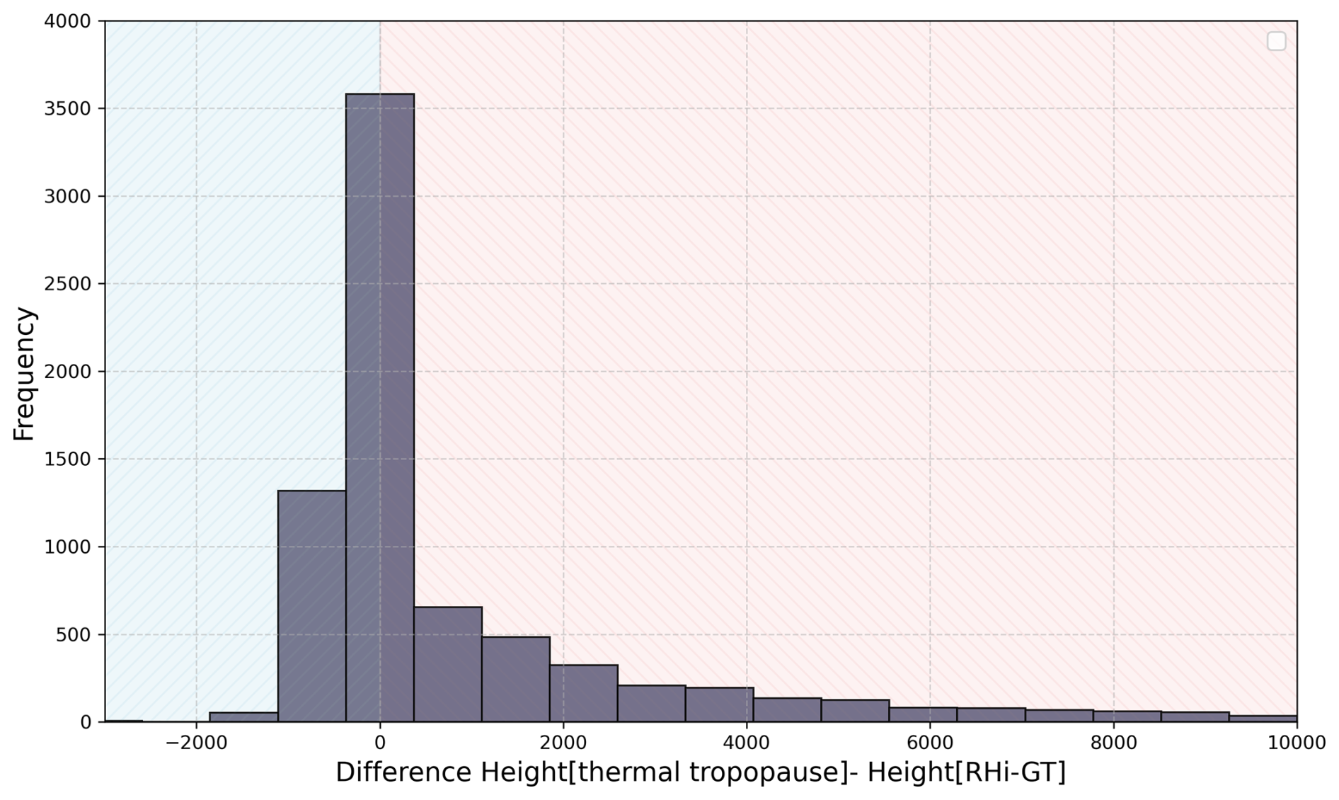
Figure 4 Histogram of the height difference in [m] between the thermal tropopause and RHi-GT. Negative values (blue shaded) denote cases, where the RHi-GT altitude is higher than the thermal tropopause. Positive differences (red shaded) denotes cases, where the RHi-GT altitude is below the thermal tropopause.

The results clearly show that most tropopause heights based on RHi-GT are in a similar range than the heights obtained by the WMO criterion. The deviation towards negative height differences, i.e. RHi-GT height is larger than the thermal tropopause, is limited by the dry stratosphere, as in this layer the relative humidity over ice falls below the threshold required for the RHi-GT definition. Therefore, the RHi-GT is not expected to be much higher than the thermal tropopause. On the other hand, the histogram shows for positive difference values an elongated tail, i.e. for cases of RHi-GT heights lower than the thermal tropopause. Especially when the thermal tropopause is quite high, the heights of the two types of tropopause can differ largely, as for example in Fig. 2, where a high thermal tropopause is found, while the RHi-GT, showing a more physically consistent picture, is about 5 km lower.

3.3 Thermodynamic variables relative to the tropopause

We now investigate some general features of the RHi-GT in comparison to the general definition of the thermal tropopause (TTP). In the following we investigate the variables RHi, absolute temperature, potential temperature and static stability (i.e. the Brunt-Vaisala frequency), respectively. We investigate the full data set of 10 years radiosonde data from Meiningen, Germany. The radiosonde data show great variability between individual ascents and thus reflect the variability of the weather. Therefore, observations of the tropopause are often carried out by means of the transformation to a tropopause-relative height grid (as, e.g., introduced by Birner et al., 2002). This means that the tropopause level is defined as zero, negative altitude values describe the troposphere, and positive values denote the stratosphere; we evaluate the profiles normalized relative to the RHi-GT and the TTP, respectively.

Figure 5 presents the mean RHi profiles relative to the two tropopause definitions. The left panel shows the results with respect to the RHi gradient tropopause (RHi-GT). First, by design, we clearly see a distinct vertical gradient in RHi that captures the abrupt shift between the moist troposphere and the dry stratosphere. There is a strong contrast between the moist troposphere (mean values RHi ∼ 60 %–80 %) and the very dry stratosphere (values below RHi ∼ 10 %), leading to a clear separation of the two spheres. Second, we find enhanced (mean) values of RHi in the troposphere, however close to the RHi-GT; the mean value has its maximum value at RHi ∼ 75 % just below the tropopause. This is in clear agreement with former investigations of ice supersaturation in the troposphere; the highest values of RHi (and thus ice supersaturation) are often found just below the tropopause, within about 0.5–1 km (Spichtinger et al., 2003; Peter et al., 2006; Reutter et al., 2020; Krämer et al., 2020). The large spread of the standard deviation in the troposphere reflects the meteorological variability during the course of 10 years.

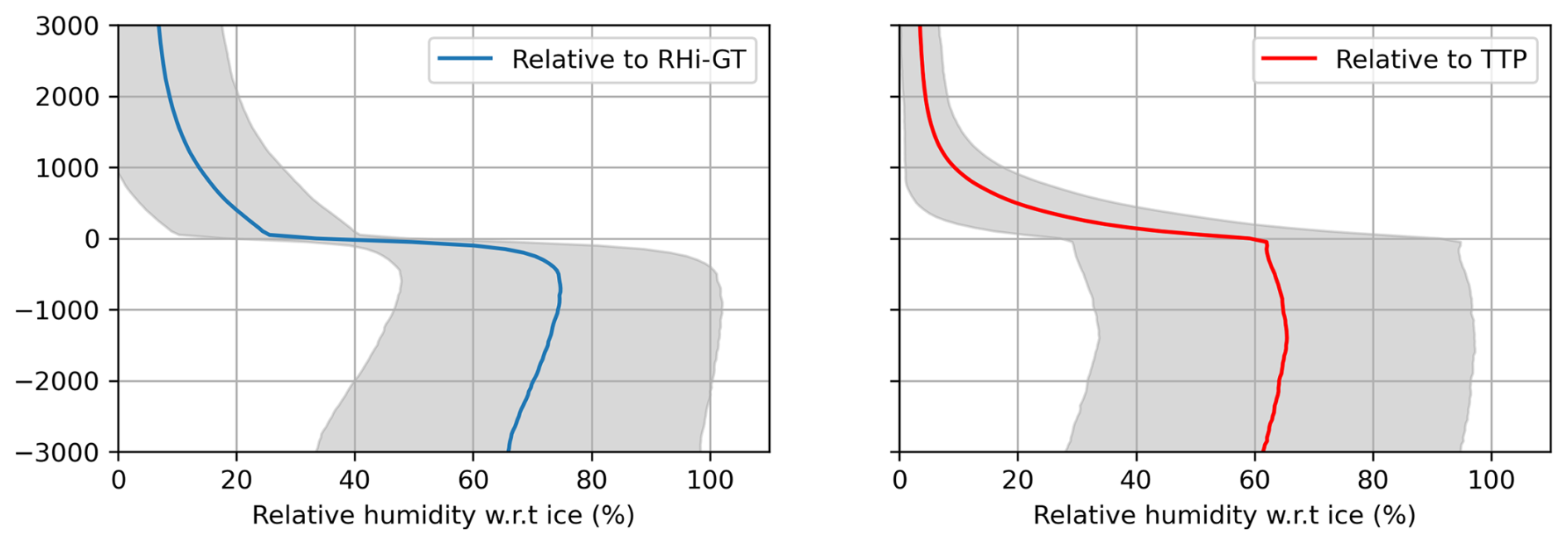
Figure 5 Mean of relative humidity over ice for (left) relative to the RHi-GT and (right) relative to the thermal tropopause. Shading denotes the range of the standard deviation.

The right panel of Fig. 5 shows the result for the widely used thermal tropopause. While the overall picture is similar to the RHi-GT evaluation, significant differences due to the different coordinate system, i.e. sampling, to the RHi-GT coordinate system are obvious. First, the transition from troposphere to stratosphere is less pronounced with a broader transition layer. The mean profile shows also a distinctive kink in the RHi curve for the thermal tropopause, while the transition in the RHi-GT case is somewhat smoother. Second, the mean values of RHi in the troposphere stay at lower values (maximum at RHi = 62 %) and the signature of highest values of RHi close to the tropopause is not visible.

Finally, it is also noteworthy, that in the RHi-GT case the stratosphere is immediately drier compared to the TTP case. This is also showing the applicability of RHi-GT as a useful measure for questions concerning water vapor, clouds and, their radiative impact on climate, since for radiation effects strong vertical gradients lead to the strongest signals in radiative heating (see, e.g., Fusina and Spichtinger, 2010).

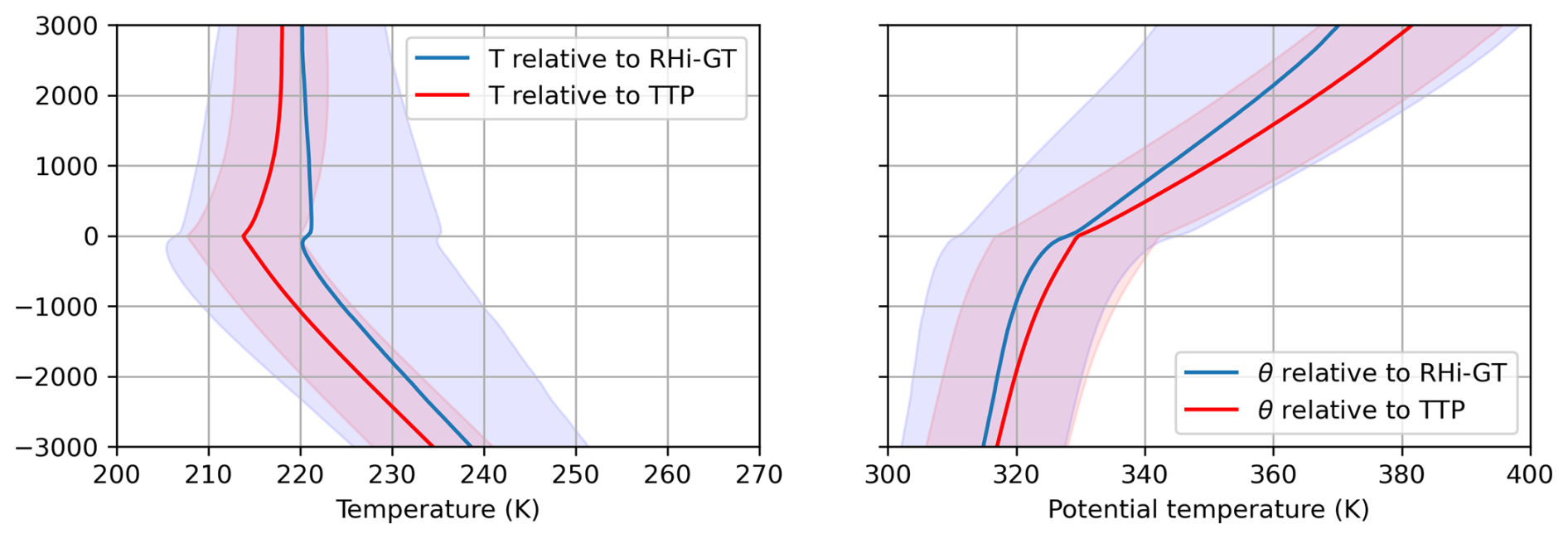
Figure 6 Mean of the (left) absolute temperature and (right) potential temperature relative to the tropopause. Blue color denote the results for the RHi-GT, while red colors denote the results relative to the TTP. Shading denotes the range of the standard deviation.

In a next step we investigate the (physical) temperature profiles. The absolute temperature profiles are displayed in the left panel of Fig. 6. The profiles for both tropopause types looks quite similar in the troposphere. Just below the height of the RHi-GT a small increase in the absolute temperature is visible, while above the temperature stays more or less constant. In contrast, by design, the results for the thermal tropopause shows the typical minimum of the absolute temperature at tropopause level. Above the thermal tropopause an increase of the temperature can be observed. We clearly see again two features for the RHi-GT in comparison to the classical TTP. First, the mean profile is shifted toward higher temperatures, with the mean RHi-GT temperature about 5 K higher than that of the thermal tropopause. While RHi-GT generally occurs at similar heights as the thermal tropopause (3580 cases, see Fig. 4), more cases are found below (2496) than above (1382) the thermal tropopause. Since temperatures increase with decreasing altitude, RHi-GT tropopauses located below the thermal tropopause naturally exhibit higher temperatures, explaining the observed mean temperature increase. Second, the spread of the temperature is significantly larger for the RHi-GT definition compared to the thermal tropopause definition. This is in accordance with the generally higher variation of RHi-GT tropopause heights, as indicated in Fig. 4.

The right panel of Fig. 6 shows the potential temperature for both tropopause definitions. Complementary to the shift in the absolute temperature profile, we see a shift to lower values for the transformed potential temperature profile of RHi-GT compared to TTP; this is consistent with the generally lower levels of RHi-GT tropopause. Similarly, the spread is also higher in the RHi-GT case. However, the potential temperature shows at the tropopause level almost the same values in both averaged profiles. In the qualitative comparison of the profiles in terms of lapse rates we find similar lapse rates in the troposphere; however, for the stratosphere the RHi-GT lapse rate is smaller. Since in case of RHi-GT the distinction between layers is related to the humidity rather than to the thermal structure as for the TTP, this is consistent and meaningful. Finally, the transition between troposphere and stratosphere for the RHi-GT definition is smoother and does not show a bend as it is the case for the TTP definition.

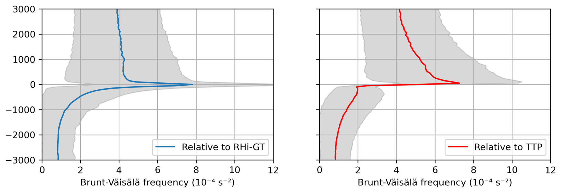
Figure 7 Mean of Brunt-Väisälä frequency squared N² for (left) relative to the RHi-GT and (right) relative to the thermal tropopause. Shading denotes the range of the standard deviation.

Finally, we investigate the static stability of the tropopause region, measured by the squared Brunt-Väisälä frequency $N^{\mathrm{2}}:=\frac{g}{\mathit{\theta }}\frac{\partial \mathit{\theta }}{\partial z}$. A general feature of stability, and thus a transport obstacle, is the so-called tropopause inversion layer (TIL, first defined by Birner et al., 2002), which appears for TTP right on top of the tropopause level. The static stability shows a strong increase over a short vertical distance. In contrast to former investigations (Birner et al., 2002; Birner, 2006) we use the newly defined RHi-GT as the reference point for the coordinate system; both versions (normalized to RHi-GT and TTP) are shown in Fig. 7 (left: RHi-GT, right: TTP).

The difference of the N² profile shows clear differences between the tropopause definitions. The N² profile relative to the RHi-GT displays a smooth increase from tropospheric values of $N^{\mathrm{2}}\approx \mathrm{1}\times {\mathrm{10}}^{-\mathrm{4}}$ s⁻². However, the vertical gradient of N² is increasing strongly up to the maximum of $N^{\mathrm{2}}\approx \mathrm{8}\times {\mathrm{10}}^{-\mathrm{4}}$ s⁻² right on the RHi-GT tropopause level. From this point upwards there is a strong and fast decrease to mean values of $N^{\mathrm{2}}\approx \mathrm{4}\times {\mathrm{10}}^{-\mathrm{4}}$ s⁻². Thus, we see a clear separation of the two spheres, with a strong increase in the stability (i.e. the TIL) right at the RHi-GT tropopause level.

The original definition of the TIL using the thermal tropopause shows a structurally more complex pattern directly below the thermal tropopause. While the tropospheric values of the Brunt-Väisälä frequency are similar for both tropopause definitions and thus normalized profiles, a noticeable kink is visible at the local minimum of $N^{\mathrm{2}}\approx \mathrm{2}\times {\mathrm{10}}^{-\mathrm{4}}$ s⁻². This kink can be seen in many studies regarding the TIL (Birner et al., 2002; Gettelman et al., 2011; Köhler et al., 2024). Starting from this kink, N² rises sharply and then reaches its maximum 50 m above the thermal tropopause with $N^{\mathrm{2}}\approx \mathrm{7}\times {\mathrm{10}}^{-\mathrm{4}}$ s⁻². In contrast, for the RHi-GT definition, the N² maximum coincides with the tropopause level itself. Above this level, N² decreases more gradually for the thermal tropopause definition than for RHi-GT, leading to similar values only about about 3000 m higher.

These differences suggest that the RHi-GT and thermal tropopause definitions emphasize different structural aspects of the TIL. While the RHi-GT-based profiles appear smoother and more vertically confined, the thermal tropopause definition highlights a more extended transition region.

Overall, we see that the separation between tropospheric and stratospheric N² values is better represented by the new RHi-GT definition than by the thermal tropopause definition, which constitutes an additional benefit for studies of the tropopause region. At the same time, interesting differences between the profiles remain, which merit further investigation beyond the scope of this study.

4 Sensitivity of RHi-GT to threshold selection

The characteristics of the RHi-GT obviously depend on the choice of the two specified threshold values. On the one hand, an RHi threshold value must be exceeded before the vertical RHi gradient is searched for. On the other hand, the determination of the RHi-GT tropopause depends strongly on the choice of the gradient itself.

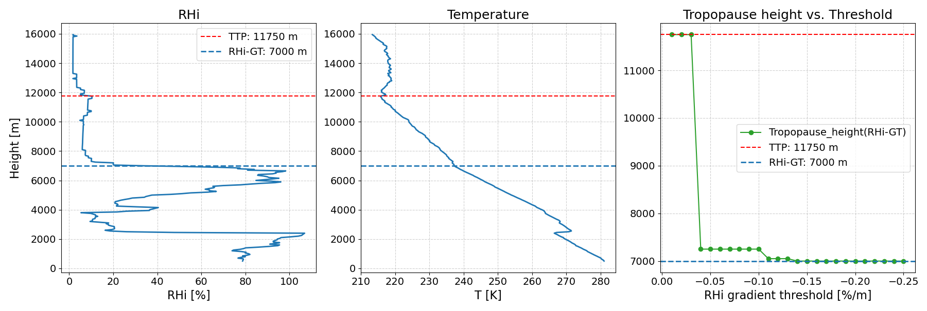
Figure 8 Dependence of the tropopause height on the choice of the vertical RHi gradient for the same case as in Fig. 2. The left panel shows the RHi profile, the absolute temperature is shown in the middle and the tropopause dependence on the RHi gradient is shown in the right panel (note the different vertical axis in this panel). For comparison, the thermal tropopause (red) and the RHi-GT with a RHi gradient of −0.15 % m⁻¹ used in this study for the previous evaluation is marked in blue.

Figure 8 shows the influence of the vertical RHi gradient on the determination of the RHi-GT height using the case from Fig. 2. The red dotted line marks the thermal tropopause, while in blue the RHi-GT with a RHi gradient of −0.15 % m⁻¹, as used in this study for the previous evaluation, is presented. In this example, the same tropopause height is obtained for a very low RHi gradient (less than −0.04 % m⁻¹) as for the WMO criterion. However, the tropopause height based on the RHi-GT decreases with a gradient between −0.04 % m⁻¹ to −0.10 % m⁻¹ by 4500 m; thus, this small feature in RHi is enough to act as a significant gradient. From an RHi gradient of more than −0.10 % m⁻¹, the tropopause height decreases slightly by another 200 m, and from −0.14 % m⁻¹ by another 50 to 7000 m. The last-mentioned tropopause altitude then remains constant over the remaining variation of the RHi gradients.

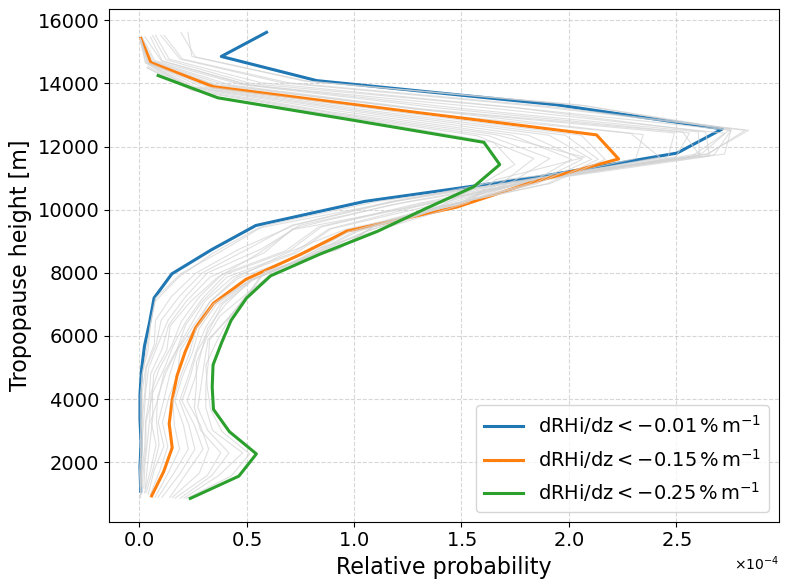
Figure 9 Tropopause height histogram depending on the choice of the vertical RHi gradient for the 10 year time period. The weakest vertical RHi gradient threshold of −0.01 % m⁻¹ is shown in blue, the RHi gradient used for the previous evaluation in this study of −0.15 % m⁻¹ is shown in orange. In green the strongest RHi gradient of −0.25 % m⁻¹ used in this sensitivity evaluation is shwon. The values in between are displayed in grey in increments of 0.01 % m⁻¹.

After considering the influence of the choice of RHi gradient on a case study, we consider now the differences for the tropopause height for the entire 10-year period of this study.

Figure 9 shows a histogram of the tropopause height for different vertical RHi gradients from −0.01 % m⁻¹ to −0.25 % m⁻¹ in steps of −0.01 % m⁻¹. The weakest (blue) and strongest gradients (green) are highlighted as well as the value of −0.15 % m⁻¹ used for the previous investigations in this study.

This clearly demonstrates the influence of the threshold value for the vertical RHi gradient on the determination of tropopause height. When the tropopause is identified using a very weak RHi gradient (blue in Fig. 9), an increased occurrence of high tropopause levels is observed in the uppermost height intervals, with the distribution maximum being the highest among all cases considered. Conversely, when the criterion is tightened to very strong RHi gradients (green in Fig. 9), the threshold is sometimes only exceeded further down in the profile when searching from above, which explains the increased frequency of very low tropopause heights in the histogram. Taken together, these observations highlight the importance of selecting an appropriate threshold for the analysis. For the present study, which focuses on the radiosonde measurements from Meiningen (Figs. 1–7), a value of −0.15 % m⁻¹ (orange in in Fig. 9) was adopted. This threshold represents a well-balanced choice for these data, avoiding extreme high or low tropopause levels and ensuring a physically consistent representation of tropopause heights, and is therefore considered a suitable reference threshold for this specific dataset.

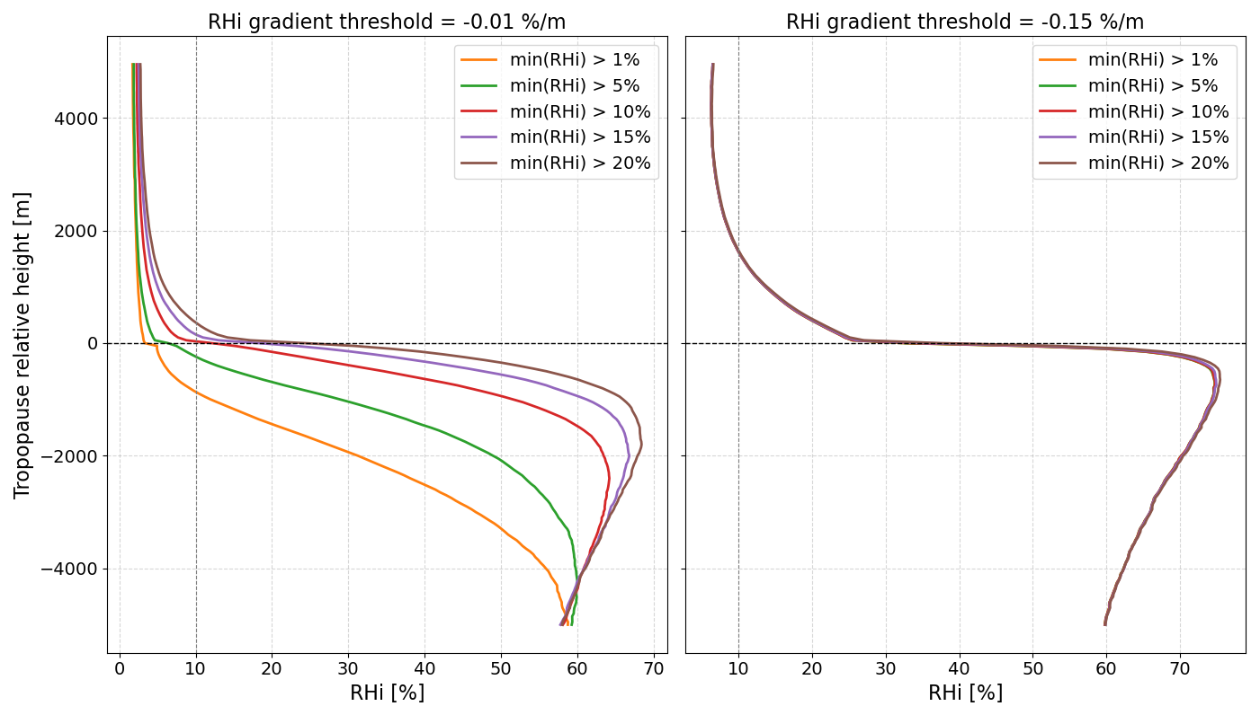
Figure 10 Influence of the minimum RHi threshold on the mean RHi profile for a weak RHi gradient threshold of −0.01 % m⁻¹ (left) and RHi gradient threshold used throughout the study of −0.15 % m⁻¹ (right). Different colours denote different minimum RHi thresholds ranging from 0 % to 20 %. The vertical axis is relative to the respective RHi-GT.

The other criterion for determining the tropopause height was the condition that RHi is above a threshold value of RHi = 10 %. Here, the results were also analyzed to determine how robust they were in relation to the choice of this threshold value. Figure 10 shows the vertical profiles of RHi. The left panel shows the results for a very weak vertical RHi gradient, while the right panel shows the results for the RHi gradient that was also used for the results in this study. It is clear to see that in the case of the very weak RHi gradient, the results, here the RHi profiles, depend very much on the choice of the minimum RHi value. In contrast, the results for a vertical RHi gradient threshold of −0.15 % m⁻¹ indicate that the choice of a minimum RHi value has a negligible impact. Nevertheless, applying a minimum RHi value can be useful in practice to account for variations in measurement quality or other data sources. The appropriate value, if any, should be determined in future studies using additional radiosonde and model datasets.

5 Summary

We present a novel approach for a tropopause definition based on the gradient of relative humidity with respect to ice (RHi). Based on high-resolution radio sonde data from Meiningen, Germany (from 2015 to 2024), we can show that the so-called RHi-GT (RHi Gradient Tropopause) definition provides a physically consistent representation of tropopause heights compared to the conventional WMO thermal tropopause. Determining the tropopause height with the help of RHi-GT is very simple. Starting at the highest available level of a radiosonde, the first gradient in RHi that exceeds a value of 0.15 % m⁻¹ is sought downwards, while the RHi itself must be at least above 10 %. In individual profiles from three different situations, the RHi-GT tropopause coincides more closely with regions that mark a clear transition in the atmosphere structure, such as sharp gradients in absolute humidity or increases in static stability. When analyzing thermodynamic variables over 10 years relative to the RHi-GT tropopause height, RHi and static stability (N²) show a more coherent transition between tropospheric and stratospheric conditions than when referenced to the thermal tropopause.

The RHi Gradient Tropopause (RHi-GT) is sensitive to the choice of threshold values, particularly the vertical RHi gradient. Very weak gradients tend to produce high tropopause levels, while very strong gradients can lead to unusually low altitudes. For the Meiningen radiosonde dataset, a gradient of −0.15 % m⁻¹ provides a balanced and physically consistent representation of tropopause heights. The choice of a minimum RHi value has little impact for this gradient, though specifying a small threshold may help account for variations in measurement quality or other datasets. Optimal values for the minimum RHi should be explored in future studies using additional radiosonde and model data.

In conclusion, we can state that the new definition of a tropopause determined from gradients of relative humidity over ice, i.e. the RHi-GT, emphasizes the boundary between layers with distinctly different water vapor characteristics. In this respect it outperforms the usual definitions relying on the thermal structure of profiles only, and is very well suited for qualitative and quantitative investigations of the tropopause region, especially including the relevant diabatic processes, as e.g. radiation and phase changes, respectively.