the Creative Commons Attribution 4.0 License.
the Creative Commons Attribution 4.0 License.
 | 30 Aug 2024
Evaluation of total column water vapour products from satellite observations and reanalyses within the GEWEX Water Vapor Assessment
Marc Schröder
Shu-Peng Ho
Steffen Beirle
Ralf Bennartz
Eva Borbas
Christian Borger
Helene Brogniez
Xavier Calbet
Elisa Castelli
Gilbert P. Compo
Wesley Ebisuzaki
Ulrike Falk
Frank Fell
John Forsythe
Hans Hersbach
Misako Kachi
Shinya Kobayashi
Robert E. Kursinski
Diego Loyola
Zhengzao Luo
Johannes K. Nielsen
Enzo Papandrea
Laurence Picon
Rene Preusker
Anthony Reale
Lei Shi
Laura Slivinski
Joao Teixeira
Tom Vonder Haar
Thomas Wagner
Since 2011, the Global Energy and Water cycle Exchanges (GEWEX) Water Vapor Assessment (G-VAP) has provided performance analyses for state-of-the-art reanalysis and satellite water vapour products to the GEWEX Data and Analysis Panel (GDAP) and the user community in general. A significant component of the work undertaken by G-VAP is to characterise the quality and uncertainty of these water vapour records to (i) ensure full exploitation and (ii) avoid incorrect use or interpretation of results. This study presents results from the second phase of G-VAP, where we have extended and expanded our analysis of total column water vapour (TCWV) from phase 1, in conjunction with updating the G-VAP archive. For version 2 of the archive, we consider 28 freely available and mature satellite and reanalysis data products, remapped to a regular longitude–latitude grid of 2° × 2° and on monthly time steps between January 1979 and December 2019. We first analysed all records for a “common” short period of 5 years (2005–2009), focusing on variability (spatial and seasonal) and deviation from the ensemble mean. We observed that clear-sky daytime-only satellite products were generally drier than the ensemble mean, and seasonal variability/disparity in several regions up to 12 kg m−2 related to original spatial resolution and temporal sampling. For 11 of the 28 data records, further analysis was undertaken between 1988–2014. Within this “long period”, key results show (i) trends between −1.18 ± 0.68 to 3.82 ± 3.94 kg m−2 per decade and −0.39 ± 0.27 to 1.24 ± 0.85 kg m−2 per decade were found over ice-free global oceans and land surfaces, respectively, and (ii) regression coefficients of TCWV against surface temperatures of 6.17 ± 0.24 to 27.02 ± 0.51 % K−1 over oceans (using sea surface temperature) and 3.00 ± 0.17 to 7.77 ± 0.16 % K−1 over land (using surface air temperature). It is important to note that trends estimated within G-VAP are used to identify issues in the data records rather than analyse climate change. Additionally, breakpoints have been identified and characterised for both land and ocean surfaces within this period. Finally, we present a spatial analysis of correlations to six climate indices within the long period, highlighting regional areas of significant positive and negative correlation and the level of agreement among records.
- Article
(14504 KB) - Full-text XML
-
Supplement
(15643 KB) - BibTeX
- EndNote


Water vapour is the most important greenhouse gas in the Earth's climate system, acting as the predominant source of infrared opacity for the clear-sky atmosphere (Douville et al., 2021). While directly and indirectly influencing radiative balance (Colman and Soden, 2021; Forster et al., 2021), surface fluxes and soil moisture, it is sufficiently abundant and short-lived that it is considered under natural control (Sherwood et al., 2010). With prevalent positive feedback on the Earth's climate system (1.2–1.4 W m−2 °C−1; Forster et al., 2021), water vapour exerts the largest amplification mechanism for anthropogenic climate change (Held and Soden, 2000; Chung et al., 2014). While water vapour in the free troposphere plays a more important role in feedback strength than lower tropospheric moisture, the link between total column water vapour (TCWV), precipitation, downward longwave radiation and atmospheric absorption of sunlight plays a key role in energy–water cycle coupling (Douville et al., 2021; Fowler et al., 2021). Therefore, water vapour is a key parameter for the Earth's energy budget and climate analysis.
In 2011 the Global Energy and Water cycle Exchanges (GEWEX) Water Vapor Assessment (G-VAP) was initiated by the GEWEX Data and Analysis Panel (GDAP) with a remit to characterise the performance of state-of-the-art water vapour products to support these type of analyses. Therefore, the scope of G-VAP activities is to highlight the strengths, differences and limitations of water vapour climate data records through consistent evaluation and intercomparison studies. The stability of long-term datasets is a key focus of the assessment. Through these activities, G-VAP supports the selection process of suitable water vapour data records by GDAP and the general climate analysis community (further details are available from http://www.gewex-vap.org, last access: 29 September 2023). Phase 1 of G-VAP concluded in 2017 with the publication of a World Climate Research Programme (WCRP) report (Schröder et al., 2017a) and an archive of TCWV, specific humidity and temperature profiles used within the analysis (Schröder et al., 2018).
In 2018, the assessment entered its second phase, focusing on the following objectives:
-
The characterisation of water vapour data records,
-
Informing users of issues within water vapour data products,
-
Climate and process-oriented analysis,
-
Continuing to link to key scientific questions and focusing on process evaluation studies (denoted PROES),
-
Enhancing regional analyses.
These objectives are similar to the objectives from the first phase by only enhancing efforts directed towards process evaluation studies and regional analysis. In particular, as in phase 1 of G-VAP, the assessment effort focuses on characterising the fitness of the various data records for climate analysis. In this study, we present the evaluation of satellite and reanalysis of TCWV records collected for the second release of the G-VAP data archive. Section 2 briefly introduces the water vapour records that make the new archive. The methods used for evaluating the archive of TCWV records are outlined in Sect. 3, with the results shown in Sect. 4. Finally, we discuss our findings within the context of the assessment (Sect. 5) and present our conclusions with recommendations in Sect. 6.
To support efforts within the second phase of the assessment, the G-VAP data archive has been updated to include new versions and products. It has been extended to cover the period from January 1979 to December 2019. The year 1979 was chosen as a starting point as it coincided with the launch of the NOAA-6 satellite, which carried a multispectral atmospheric sounding package that continues to the present day with various instrument modifications. Monthly mean fields for individual products have been processed onto a common spatial grid of 2° × 2° and values are left undefined where the archive temporal range exceeds the original coverage. Including a new flag within the archive files allows the user to select valid data. Further details on the archive preparation are given in Sect. 3.1. Within the time range covered by the archive, we define two main analysis periods:
-
The 5-year “common period” between 2005–2009 captures all products.
-
The “long period” runs from 1988–2014 and is designed to represent the Atmospheric Model Intercomparison Project (AMIP) period from the latest Sixth Assessment Report (AR6).
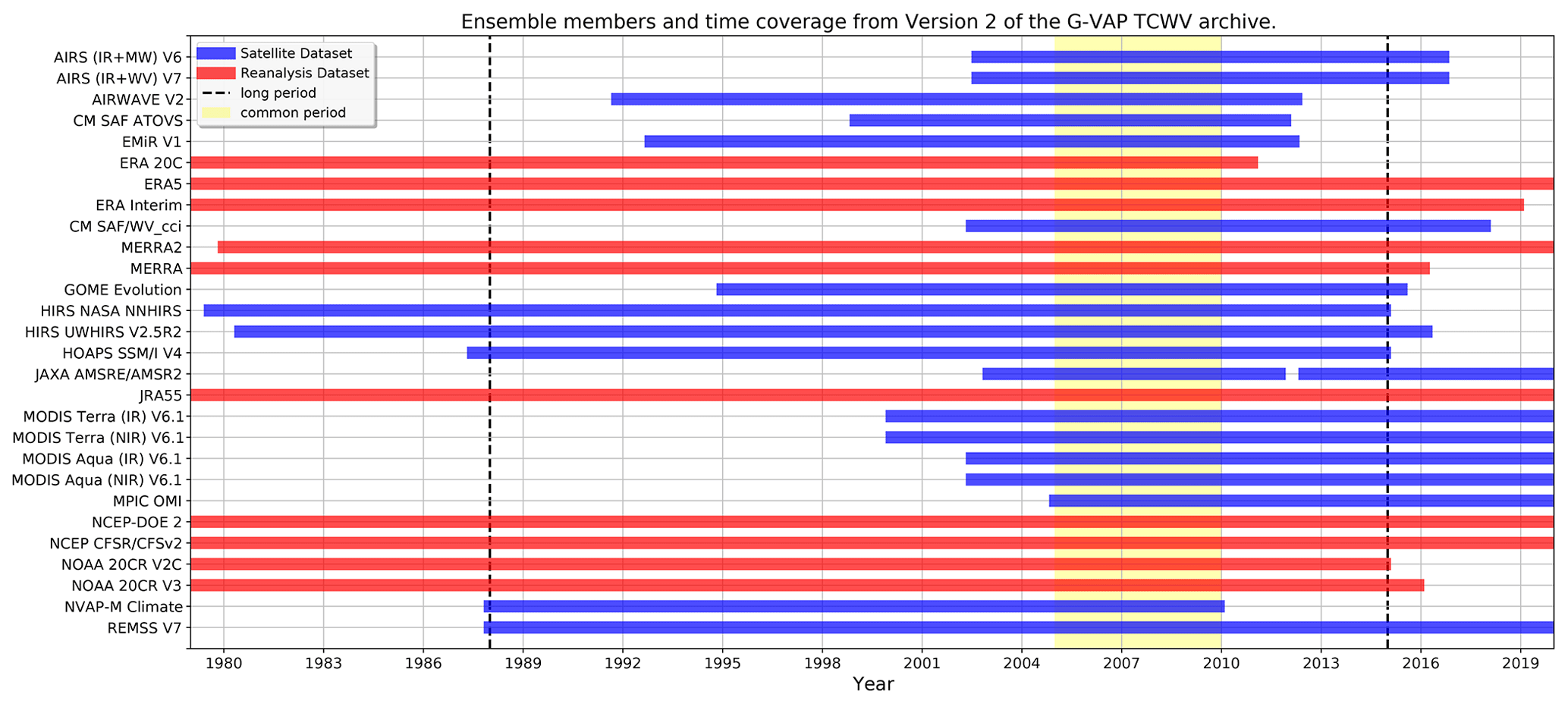
Figure 1Coverage of TCWV records included in version 2 of the G-VAP archive from 1 January 1979 to 31 December 2019. Satellite records are shown in blue, whilst reanalyses are indicated in red. The two analysis periods, long (1 January 1988 to 31 December 2014) and common (1 January 2005 to 31 December 2009), are represented by black dashed lines and the yellow shaded region, respectively.
In the rest of this section, we detail which records are newly added products and which have been updated/extended. An overview of included products within version 2 of the G-VAP archive and analysis periods is shown in Fig. 1. The archive is expected to be released with the second G-VAP report in 2025. It should be noted that all water vapour records will have limitations based on their underlying assumptions or operational frameworks. For example, satellite sensors can experience degradation (often corrected through recalibration efforts, e.g. Tabata et al., 2019) from the reduction of the sensitivity of an instrument over time, while reanalysis records can experience shifts in the time series due to changes in observing systems assimilated (Schröder et al., 2017a; Allan et al., 2022). Individual data record performance assessments are usually detailed in publications or via technical documents such as the “Product User Guide” (PUG) or “Validation Report” (VR) and are not provided here. Through the assessment, we can highlight performance issues (e.g. breakpoints) and attempt to map them to known issues. Where we cannot identify the cause, our results can be used by the data record teams in future product updates.
2.1 Updated and new records within version 2
The starting point for this study was the previous version of the G-VAP data archive (Schröder et al., 2018) with 22 satellite and reanalysis TCWV records. These records were initially split into three categories: (i) records with no version update but extended time series, (ii) records with a newer version (superseded), or (iii) records with no updates in version or temporal coverage. From the initial set of records, 18 datasets fell into the first two categories, with 14 being retained and extended and 4 being updated to newer versions. In the case of the Moderate Resolution Imaging Spectroradiometer (MODIS) products, we now include the Terra and Aqua versions, i.e. MOD08_M3 (new) and MYD08_M3 (as in the previous archive), respectively. Short abstracts for these datasets are given in Schröder et al. (2018) and are not repeated here; however, details of these datasets are given in Table 1. Finally, 10 further satellite and reanalysis records are added to the archive, with some including different versions of the same product if they were both available at the time of this study (e.g. AIRS v6 and v7). The following Sect. 2.1.1 to 2.1.8 provide abstracts for each new product in the archive.
(Castelli et al., 2019)Table 1Details of data records from version 1 of the G-VAP archive and their status within the version 2 release. Version 1 of the archive is available from https://doi.org/10.5676/EUM_SAF_CM/GVAP/V001 (Schröder et al., 2017b).
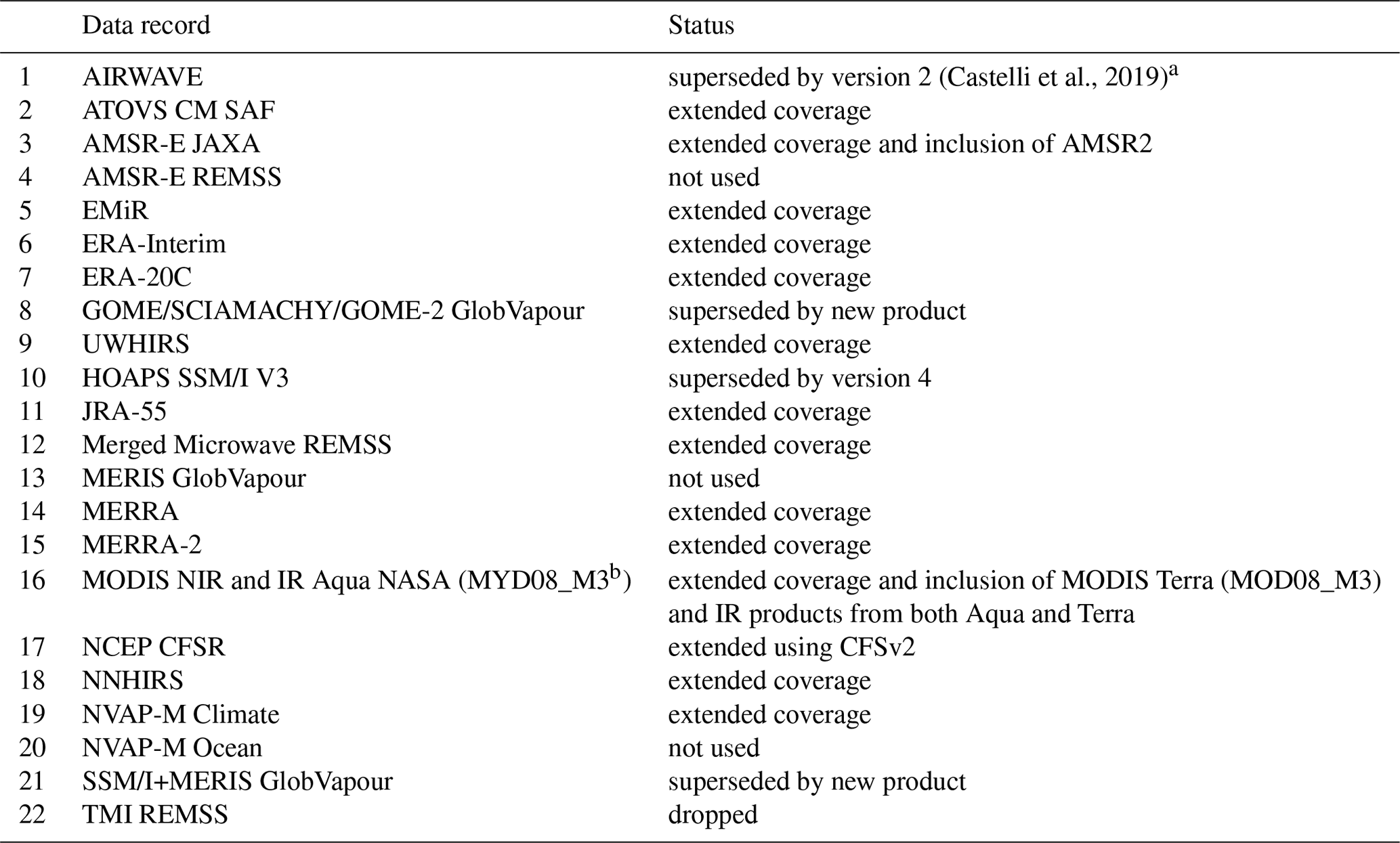
a The AIRWAVEv2 data are available on request from Elisa Castelli (e.castelli@isac.cnr.it) and Enzo Papandrea (e.papandrea@isac.cnr.it). b Only NIR TCWV data used in version 1 of the archive.
2.1.1 AIRS
On board the National Aeronautics and Space Administration's (NASA) Aqua platform (13:30 local time, LT; 01:30 h local overpass time), the Atmospheric Infrared Sounder (AIRS) produces a range of geophysical products, including cloud-cleared radiances, temperature and water vapour profiles, cloud properties, methane, carbon monoxide, ozone, and surface temperature. While retrievals can be done with AIRS infrared (IR) radiances alone, this study utilises output from combined AIRS IR and microwave (MW) observations from the Advanced Microwave Sounding Unit (AMSU). This configuration, known as the “golf ball”, collocates nine AIRS footprints (3 × 3) within an AMSU field of regard (FOR) and assumes the scene to be homogeneous except for cloud amount. The algorithm compensates for the cloud effects on the IR radiances within the scene before being passed to the final retrieval stages. Further details can be found in Susskind et al. (2003) and Susskind et al. (2020). In this study, we use the AIRX3STM monthly mean TCWV record (AIRS Science Team and Teixeira, 2013; AIRS project, 2019), which integrates the AIRS L2 water vapour profile to create a column measurement before being averaged over the month on a 1° × 1° grid for both the ascending (South Pole to North Pole) and descending (North Pole to South Pole) nodes of the orbit (day and night, respectively). We have averaged both ascending and descending monthly data for the monthly mean used in this study. While the Aqua platform has been in orbit for 20 years, this data record only runs between 30 August 2002 through to 24 September 2016 due to the failure of the AMSU-A2 module.
2.1.2 CM SAF/WV_cci
The global TCWV data record combines microwave (MW) and near-infrared (NIR) imager-based TCWV data over the ice-free ocean and over land and coastal ocean and sea ice, respectively. The data record relies on MW observations from the Special Sensor Microwave Imager and Sounder (SSM/I, SSMIS), Advanced Microwave Scanning Radiometer for EOS (AMSR-E) and Tropical Rainfall Measuring Mission's Microwave Imager (TMI). The level 1b (L1b) MW product used over global ice-free oceans is partly based on a fundamental climate data record (Fennig et al., 2020), generated within the European Organisation for the Exploitation of Meteorological Satellites' (EUMETSAT) Satellite Application Facility on Climate Monitoring (CM SAF). Equator crossing times of microwave imagers are shown at https://www.remss.com/support/crossing-times/ (last access: 22 September 2023). While over land surfaces, NIR L1b measurements from the MEdium Resolution Imaging Spectrometer (MERIS, third reprocessing), MODIS-Terra (collection 6.1), and Ocean and Land Colour Instrument (OLCI, first reprocessing) are used, each with an approximate Equator crossing time at 10:30 LT. The NIR and MW TCWV observations are combined within the Water Vapour project of the European Space Agency's (ESA) Climate Change Initiative (WV_cci). Details of the retrievals are described in Andersson et al. (2010) and Andersson et al. (2017) for the MW imagers as well as in Lindstrot et al. (2012), Diedrich et al. (2015) and Fischer et al. (2021) for the NIR imagers. The atmosphere's water vapour is vertically integrated over the full column and given in units of kg m−2. The MW and NIR data streams are processed independently and combined afterwards by not changing the individual TCWV values and their uncertainties. The data record has a spatial resolution of 0.5° × 0.5° (and 0.05° × 0.05°), with the NIR-based data being averaged and the microwave-based data being oversampled to match the 0.5°, (respectively 0.05°) spatial resolution. The product is available as daily and monthly means and covers the period from July 2002–December 2017. The data are subsequently referred to as the CM SAF/WV_cci data record and is referenced and accessible via the following DOI: https://doi.org/10.5676/EUM_SAF_CM/COMBI/V001 (Schröder et al., 2023).
2.1.3 GOME EVOL
The “GOME evolution climate” product was generated within the GOME Evolution project funded by ESA, and the retrieval is described in detail in Beirle et al. (2018a). It is based on measurements from the satellite instruments Global Ozone Monitoring Experiment (GOME), SCanning Imaging Absorption spectroMeter for Atmospheric CHartographY (SCIAMACHY) and GOME-2 in the red part of the visible spectral range, using the retrieval proposed in Wagner et al. (2003, 2006), with all satellite measurements (daytime only) occurring around 10:00 LT. As stated in Beirle et al. (2018a), a particular focus of the climate product is the consistency amongst the different sensors to avoid jumps from one instrument to another. This is reached by applying robust and simple retrieval settings consistently. Potentially systematic effects due to differences in ground pixel size are avoided by merging SCIAMACHY and GOME-2 observations to the GOME spatial resolution, allowing for a consistent treatment of cloud effects. In addition, the GOME-2 swath is reduced to that of GOME and SCIAMACHY to have consistent viewing geometries. The remaining systematic differences between the sensors are investigated during overlap periods and corrected in the homogenised time series. The GOME evolution climate product contains monthly mean TCWV from July 1995 to December 2015 on a 1° spatial resolution. It is available at https://doi.org/10.1594/WDCC/GOME-EVL_water_vapor_clim_v2.2 (Beirle et al., 2018b).
2.1.4 ERA5
The European Centre for Medium-Range Weather Forecasts (ECMWF) Reanalysis v5 (ERA5) atmospheric general circulation model and 4D-Var assimilation system are based on the IFS Cycle 41r2 and IFS Cycle 41r2 4D-Var versions of the ECMWF Integrated Forecast System (IFS). It is conducted at a resolution of about 31 km in the horizontal and 137 levels in the vertical from the surface to 0.01 hPa, and the analysis is available at a 1 h temporal resolution. ERA5 is the successor of the ERA-Interim reanalysis. Among others, ERA5 exhibits significant improvements in resolution, including a 10-member ensemble of data assimilation and various additional parameters, and it incorporates an improved 4D-Var and variational bias correction scheme through the utilisation of (newly reprocessed) datasets and recent instruments. ERA5 exploits a vast number of datasets, including in situ measurements from land stations as well as measurements from ships and drifting buoys, radiosondes, pilot balloons, aircraft, and wind profilers. The largest amount of data comes from satellite observations, focusing on polar-orbiting and geostationary satellites and improvements in all-sky assimilation. In fact, ERA5 assimilates most of the satellite measurements considered in this study (see Hersbach et al., 2020, Table 4 and Fig. 5). ERA5 provides complete atmospheric products globally from 1940 onwards at a mixed hourly/3-hourly output frequency and is continued with updates in near real-time. ERA5 and its quality are described in Hersbach et al. (2020). Monthly means of TCWV with a spatial resolution of 2° × 2° were downloaded from https://doi.org/10.24381/cds.f17050d7 (Hersbach et al., 2023) in November 2020.
2.1.5 MODIS TIR NASA (Aqua and Terra)
In addition to the MODIS NIR TCWV data, the second TCWV record based on NASA's Moderate Resolution Imaging Spectroradiometer (MODIS) used in this study is the atmospheric profile product MYD07_L2/MOD07_L2 (Aqua/Terra, respectively). This product uses the thermal infrared (TIR) bands 25 and 27 through 36 to retrieve temperature and moisture profiles, total-ozone burden, atmospheric stability, and atmospheric water vapour for daytime (10:30, 13:30 LT) and night-time (22:30, 01:30 LT) overpasses (Terra/Aqua, respectively). The level 2 (L2) product contains the geophysical parameters at a resolution of 5 × 5 km for both clear-sky day and night scenes. A scene is considered clear if at least nine 1 × 1 km pixels are cloud free, for which the MODIS cloud mask (MOD35_L2) is used for screening. The retrieval algorithm uses a modified version of the International TOVS Processing Package (ITPP) (where TOVS is the TIROS Operational Vertical Sounder, where TIROS is the Television and InfraRed Observation Satellite) for which the initial state vector uses a linear regression first-guess approach (Seemann et al., 2003; Borbas et al., 2011). Monthly mean fields gridded at 1° × 1° are available within collection 6.1 of the MOD08_M3/MYD08_M3 L3 product, which is also used for the source of the MODIS NIR TCWV product from version 1 of the archive. The level-3 MODIS MYD08 and MOD08 products can be obtained from the NASA Level-1 and Atmosphere Archive and Distribution System (LAADS) Distributed Active Archive Center (DAAC), Goddard Space Flight Center, Greenbelt, MD, USA (https://doi.org/10.5067/MODIS/MYD08_M3.061, Platnick et al., 2015a; https://doi.org/10.5067/MODIS/MOD08_M3.061, Platnick et al., 2015b).
2.1.6 MPIC OMI
The TCWV dataset provided by the Max Planck Institute for Chemistry (MPIC) is based on hyperspectral satellite measurements in the visible blue spectral range from the Ozone Monitoring Instrument (OMI) on board NASA's Aura satellite with an Equator crossing time of about 13:30 LT (daytime only observations). For this dataset, the retrieval algorithm of Borger et al. (2020) has been modified to account for the specific instrumental issues of OMI (e.g. the “row anomaly”) and the inferior quality of solar reference spectra. The TCWV dataset only includes measurements for which the effective cloud fraction < 20 %, the AMF (air mass factor) > 0.1, the ground pixel is snow and ice free, and the OMI row is not affected by the row anomaly over the complete time range of the dataset. The remaining satellite measurements are then binned to a regular latitude–longitude lattice via an area-weighted gridding algorithm, covering both land and ocean surfaces globally. In-depth details about the dataset generation, sampling errors and clear-sky bias are available in Borger et al. (2023a). Moreover, the dataset has been validated with respect to reanalysis data, satellite measurements and radiosonde observations. Furthermore, a temporal stability analysis demonstrated that the MPIC OMI TCWV dataset shows no significant deviation trends and aligns with the Global Climate Observing System (GCOS) stability requirements. The water vapour of the atmosphere is vertically integrated over the full column and given in units of kg m−2. The dataset has a spatial resolution of 1° × 1° and is available as monthly means for the time range January 2005 to December 2020. The dataset is referred to as the MPIC OMI TCWV climate data record and is available via the following DOI: https://doi.org/10.5281/zenodo.7973889 (Borger et al., 2023b).
2.1.7 NCEP-DOE 2
The National Centers for Environmental Prediction (NCEP), US Department of Energy (DOE) Reanalysis 2 (NCEP-DOE 2) was originally created to support the second Atmospheric Model Intercomparison Project (AMIP). The NCEP-DOE 2 uses a global spectral model with a spatial resolution of T62 (≈ 210 km) and 28 vertical levels for both forecasts and analyses. The data assimilation uses spectral statistical interpolation (or 3D-Var) with a one-way coupled ocean model 4D assimilation (Kalnay et al., 1996). Outputs are available daily on 6 hourly time steps or as daily or monthly averages. In addition to the spectral T62 grid, geophysical parameters are also available on a regular 2.5° latitude × 2.5° longitude global grid. NCEP-DOE 2 has a number of improvements over its predecessor, with corrections for the Southern Hemisphere bogus data (PAOBS) problem between 1979–1992, snow cover and snowmelt, humidity diffusion and discontinuities, and oceanic albedo. Further details on the improvements and updates made to NCEP-DOE 2 can be found in Kanamitsu et al. (2002). One important point regarding NCEP-DOE 2 is that it does not assimilate either SSM/I, SSMIS data or TOVS/ATOVS water vapour profiles to constrain atmospheric moisture, in contrast to, for example, ERA5 which assimilates radiances from these sensors. NCEP-DOE 2 data are provided by NOAA PSL and were last accessed via https://psl.noaa.gov/data/gridded/data.ncep.reanalysis2.html (last access: 12 May 2021; Physical Sciences Laboratory, 2021; Kanamitsu et al., 2002).
2.1.8 NOAA 20CR V2C and V3
The NOAA-CIRES-DOE (National Oceanic and Atmospheric Administration, Cooperative Institute for Research in Environmental Sciences) Twentieth Century Reanalysis (20CR) project provides a comprehensive dataset of reconstructed global weather spanning over 150 years at sub-daily resolution (Compo et al., 2011). The analysis is generated by assimilating only surface pressure observations into the NCEP Global Forecast System (GFS) model with prescribed sea surface temperatures and sea-ice concentrations. Currently, two versions of 20CR are available: (i) version 2c (V2c), which runs from 1851 to 2014 on 6 hourly time steps on a 2° × 2° resolution grid, and (ii) version 3 (V3), which has an extended coverage spanning from 1806 to 2015 and a high temporal and spatial grid of 3 h and 1° × 1°, respectively (Slivinski et al., 2019, 2021). Both product versions use a deterministic ensemble Kalman filter (EnKF) for the data assimilation (Whitaker et al., 2004; Compo et al., 2011); however, V3 also includes an additional 4-dimensional incremental analysis update (Lei and Whitaker, 2016). NOAA PSL provided the NOAA 20CR data, and they were last accessed via https://www.psl.noaa.gov/data/gridded/data.20thC_ReanV3.html (last access: 3 November 2020, Physical Sciences Laboratory, 2020b).
This section describes the preparation and analysis methodologies used in this study.
3.1 Preparation of TCWV records for inclusion in the archive
For each data record used in this study, monthly mean TCWV fields were first processed onto a common grid format of 2° × 2° between January 1979 and December 2019. The datasets were downloaded at their native resolutions and processed in one of two ways. For the reanalysis records, each monthly gridded TCWV global field was first shifted in longitude space to run between −180 to 180° before being interpolated onto the centres of the archive common grid using a linear spline function. The monthly mean level 3 (L3) satellite products were regridded if the native resolution was less than that of the common grid and averaged if separated into day/night means. All data were then written in netCDF format, with a new time flag added to indicate monthly time steps where valid data exist.
3.2 Calculation of trends
As with the first phase of G-VAP (Schröder et al., 2019), a main metric used to characterise the performance of records in the archive is the TCWV trend over the 27-year long period. It is important to note that trends estimated within G-VAP are used to identify issues in the data records rather than analysis of climate change. Before trends are calculated, global TCWV time series of ice-free oceans and land surfaces are created. For this step, a conservative mask (Fig. 2) is applied to select either ice-free ocean or land grid cells between ±60° at each monthly time step. The weighted mean TCWV at time step t () is then calculated from all valid data points (P):
where the weights w are the cosine of the latitude. Next, a level shift linear regression model (Weatherhead et al., 1998) is used to calculate the trend:
where μ is the intercept, ω is the trend, Xt is the time index, δ is the magnitude of any shift, Ut is the step function and ηt is the fit residual. For the purposes of performance analysis, the step function is assumed to be zero. However, breakpoints in the TCWV times are characterised later on. For the residuals, the same approach is used from Schröder et al. (2019) where the El Niño–Southern Oscillation (ENSO) strength and annual cycle are fitted simultaneously. The Japan Meteorological Agency (JMA) index (Bove et al., 1998), which is calculated from sea surface temperature (SST) anomalies, is used as a consistent source for the ENSO strength across all records. Figure 3a illustrates the median contribution of ENSO to TCWV variability across the 13 records spanning the long period. Positive values represent regions which see positive/negative TCWV changes for the El Niño and La Niña phases of ENSO, respectively, while the negative regions experience opposite behaviour with increases in TCWV during La Niña and a decrease during El Niño. The spread in the ENSO contribution is shown in Fig. 3b, represented by the median absolute deviation (MAD):
where E is the ENSO weight strength as a function of longitude (λ) and latitude (ϕ), and is the median ENSO strength. The largest variability is seen in the tropics, with ENSO regions seeing 10 % to 20 % variability between data records.
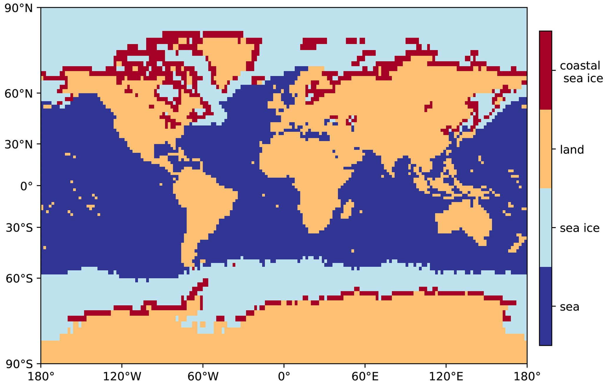
Figure 2Conservative sea-ice mask produced from a combination of the ESA CCI land cover classification and EUMETSAT OSI SAF (Ocean and Sea Ice Satellite Application Facility) sea-ice concentration products. Sea ice or coastal sea ice is flagged if any common grid cell contains detected sea ice between 1988–2014.
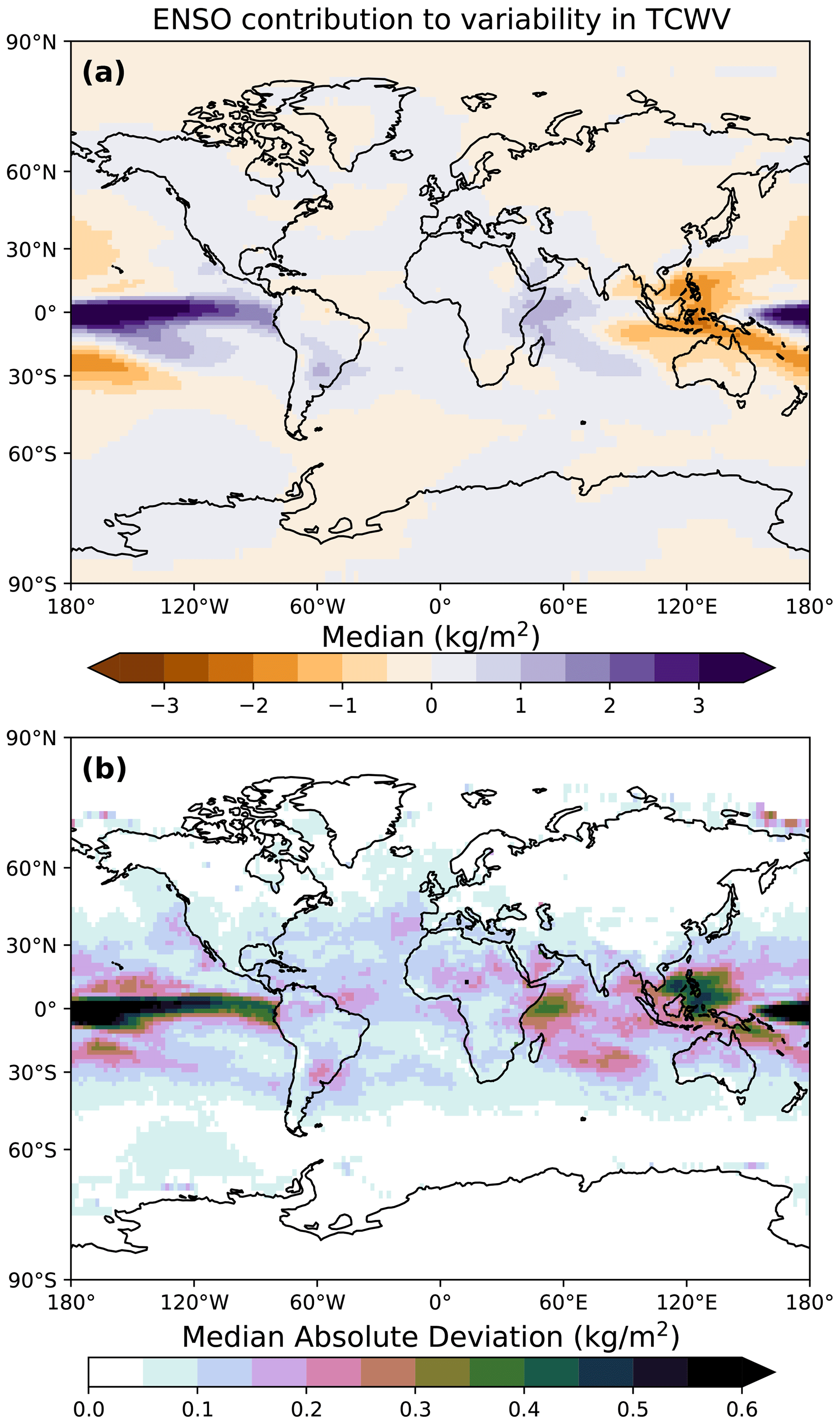
Figure 3(a) Median ENSO contribution to the variability in TCWV for all archive ensemble members that cover the common long period between 1988–2014. The median absolute deviation (MAD) for the ensemble median ENSO contribution is shown in panel (b).
3.3 Regression against surface temperatures
In addition to calculating trends, and to be consistent with phase 1 of G-VAP, a regression of each TCWV record against the surface temperature dataset(s) is performed following the approaches outlined in Dessler and Davis (2010) and Mears et al. (2007). If we assume that relative humidity (RH) is constant, then the Clausius–Clapeyron relationship produces a ratio between changes in water vapour and temperature that is only dependent on temperature. Therefore, under constant RH and pressure assumptions, changes in water vapour mixing ratios can be transferred to saturation vapour pressure values. For a temperature change of 1 K, the expected change in mixing ratio is between 6 % at 300 K and 7.5 % at 275 K. These values then provide the limits of the range of expected regression coefficients against the chosen surface temperature data records used in this study:
-
Over ocean, sea surface temperature (SST) data from the European Space Agency (ESA) Climate Change Initiative (CCI) (Merchant et al., 2019; Merchant and Embury, 2020).
-
For both land and ocean surfaces, surface air temperature (T2m) from the European Centre for Medium-Range Weather Forecasts (ECMWF) ERA5 reanalysis (Hersbach et al., 2020) is used.
Both temperature datasets were processed on the same grid as the TCWV records in the G-VAP archive for consistency.
3.4 Detection of breakpoints
The detection of breakpoints is carried out as described in Schröder et al. (2019). Here, a summary of the approaches is provided, and a few newly implemented changes are also mentioned. Two breakpoint analyses are applied: the penalised maximal F (PMF) test (Wang, 2008a, b) and a variant of the standard normal homogeneity (SNH) test (Hawkins, 1977; Alexandersson, 1986), as proposed in Reeves et al. (2007). The breakpoint analyses detect abrupt changes in the time series of TCWV, and the output of this analysis is the time and the strength associated with the breakpoint. Here, breakpoints are provided when the level of significance is 0.05. Two tests are applied to increase confidence in the case that both tests observe the same breakpoint. Input to the PMF and SNH tests are anomaly differences, i.e. after removal of the mean annual cycles, the difference between the anomalies from a data record and a reference are computed. Over the ocean, the Hamburg Ocean Atmosphere Parameters and Fluxes from Satellite data record (HOAPS) V4 was used as a reference; elsewhere, ERA5 was used. As ERA5 was already introduced in Sect. 2.1.4, we briefly recall here key characteristics of HOAPS. HOAPS is a product suite of satellite-based climate data records, including TCWV, over the global ice-free oceans. TCWV is derived from quality controlled, recalibrated, and intercalibrated measurements from SSM/I and SSMIS passive microwave radiometers (Fennig et al., 2020), except for the SST, which is taken from Advanced Very High Resolution Radiometer (AVHRR) measurements. TCWV is retrieved with a 1D-Var scheme. The data record covers the time period from July 1987 to December 2014 and has global coverage, i.e. within ±180° longitude and ±80° latitude. The product is available as monthly averages and 6-hourly composites on a regular latitude–longitude grid with a spatial resolution of 0.5° × 0.5° degrees. Using HOAPS V4 and ERA5 as references is not meant to be a sign of superior quality. Further details and comments are given in Schröder et al. (2019, 2016). The UWHIRS v2.52 data record contains undefined values in the period October–December 1990. This gap has been linearly interpolated to allow for the application of the homogeneity analysis. The interpolated data are not included in any other analysis nor in the time series plots.
3.5 Correlation to climate indices
The final test applied to archive records covering the long period is to calculate their correlation to various climate indices. With TCWV records now spanning multiple decades, it provides new opportunities to go beyond trends and study global climate signals and phenomena, e.g. teleconnections (Wagner et al., 2021). Therefore, it is vital to understand the representativeness and correlations of climate signals between different data records. The indices chosen for this study are the following:
-
Atlantic Meridional Mode (AMM). AMM is the dominant source of coupled ocean–atmosphere variability in the Atlantic.
-
Arctic Oscillation (AO). AO is the shifting atmospheric pressure back and forth between the Arctic and mid-latitude areas of the North Atlantic and Pacific oceans.
-
North Atlantic Oscillation (NAO). NAO is based on the surface sea-level pressure difference between the subtropical (Azores) high and the subpolar low.
-
El Niño–Southern Oscillation Index 3.4 (NINO3.4). NINO3.4 is one of several El Niño–Southern Oscillation (ENSO) indicators based on sea surface temperatures. NINO3.4 is the average sea surface temperature anomaly in the region bounded by 5° N to 5° S, from 170° W to 120° W.
-
Pacific Decadal Oscillation (PDO). PDO is characterised by a change in sea surface temperature in the North Pacific (north of 20° N). The change usually occurs abruptly. PDO has a higher frequency than ENSO.
-
Pacific Meridional Mode (PMM). PMM is defined as the leading mode of non-ENSO coupled ocean–atmosphere variability in the Pacific basin.
These indices are the same as those used in phase 1 of the G-VAP assessment with the addition of the PMM. Further details on each index are described in Table B1 and in the time series plotted in Fig. S1 in the Supplement. For each record, the Pearson correlation (r) is calculated between the TCWV anomalies (ΔWV) and the specific climate index (CI) for each common grid cell:
where CIt and ΔWVt are the climate index and TCWV anomaly at time step t, and μCI and μΔWV are the mean climate index and TCWV anomaly, respectively. A spatial analysis is then performed between the different records to assess the level of agreement in correlation results for each climate index. Finally, it is important to note that correlations also exist between the different climate indices; this is illustrated in Fig. 4.
Figure 4(a) Correlation coefficients between the different climate indices used in this study for the period spanning 1988 to 2014. Calculated P values for each correlation value are shown in (b), with the colour bar range set between 0 and 0.05 representing the range of α threshold values used within science. Values outside this range are set to grey and deemed not statistically significant.
Results from the analysis of TCWV records are presented here and have been split into two distinct sections: the first covers the shorter common period, and the second is a broader analysis of the longer-term records.
4.1 Evaluation of records within the common period
Figure 5 presents seasonal TCWV maps of the archive ensemble mean (μ), standard deviation (σ), coefficient of variation () and range (TCWVmax–TCWVmin) for the whole common period (2005–2009) for all 28 records. The seasons are defined as DJF (Northern Hemisphere (NH) winter), MAM (NH spring), JJA (NH summer) and SON (NH autumn) where the capitalised letter of each month (e.g. December, January, February) makes up the season acronym.
Figure 5Seasonal maps of the mean archive ensemble total column water vapour (TCWV) over the common period (2005–2009). Also included is the standard deviation of the seasonal mean (σ), the respective coefficient of variation (CV), and the difference between the seasonal maximum and minimum TCWV values (TCWVmax–TCWVmin). While the largest (absolute) variability is seen in the Tropics, the greater relative difference (> 50 %) is found in polar regions.
The column of maps presents the seasonal ensemble means, where we can observe a clear seasonal cycle with no anomalous regions immediately apparent. However, when we examine the standard deviation for each season (second column), four regions stand out with high absolute values:
-
The first is the Sahel, where we observe standard deviations ≥ 10 kg m−2 between MAM and SON.
-
The second region is the Indo-Gangetic Plain (IGP), where JJA and SON values are well above 10 kg m−2, exceeding 15 kg m−2 in some regions.
-
The northeast of China and Japan is the third region, where σ values are approximately 12 kg m−2 for NH summer and autumn months.
-
The fourth and final region is observed off the Pacific coast of Mexico. In this narrow region, variability amongst the data records is between 11–12 kg m−2 for JJA and SON.
Over the tropics and mid-latitudes, we see variability from cloud cover, which results in standard deviation values between 5–7 kg m−2. In polar regions, these drop to σ values of ≤ 1 kg m−2. However, we get a slightly different perspective on the TCWV variability by normalising the standard deviation with the seasonal mean to compute CV. The third column of Fig. 5 shows CV, where now three different areas are highlighted (where CV values > 70 %). These regions are (i) the Tibetan Plateau, (ii) the Andes, and (iii) high latitudes/polar regions. The common theme between these three is that all have dry atmospheres and variable topography, especially for the Tibetan Plateau and the Andes. The CV has a distinct intra-seasonal signal for polar regions, with the hemispherical winter exhibiting the greatest variability among the data records.
Examining the seasonal range of the archive records (Fig. 5, fourth column) reveals that areas with high standard deviations, in general, have a range of ≥ 50 kg m−2, while regions with high CV see seasonal ranges of 10–20 kg m−2. For very dry regions, 10–20 kg m−2 can be 3–10 times the season mean TCWV, whilst for tropical regions high standard deviations are associated with high monthly mean TCWV values. Therefore, this highlights a significant disagreement between the archive records for dry atmospheres, especially at high latitudes. This disagreement can be driven by either low sensitivity in observational satellite records or a lack of in situ measurements to constrain reanalyses.
The variability of TCWV observed within the archive is investigated further by comparing each record to the ensemble mean for the common period. For each dataset, the monthly difference to the ensemble mean has been calculated before being averaged over the time period. Next, these differences were summed to calculate each dataset's global value. Finally, all results were sorted from driest to wettest and shown in Fig. 6. It should be noted that here the ranking of datasets is not a statement of climate performance (i.e. bias to characterise reference/truth) but rather highlights characteristics related to differences in the observational/assimilation systems. From these global mean differences, the initial inferences we can make are the following:
-
11 datasets are drier than the ensemble mean, while the remaining 17 are wetter, with the EMiR record exhibiting the smallest global ΔTCWV (bias relative to the ensemble mean).
-
All IR and NIR TCWV records have the driest global ΔTCWV, while other MW, MW+IR and MW+NIR records sit between −2.8 % and 4.3 %.
-
The GOME Evolution and MPIC OMI products, which use the visible (blue or red) spectral region to retrieve TCWV, show very different results. Both being daytime-only products (morning vs. afternoon overpass, respectively), GOME Evolution has a ΔTCWV of 0.74 %, while MPIC OMI is much larger at 9.2 %.
-
Overall, reanalyses are wetter than the global ensemble mean TCWV except for JRA55 and ERA 20C.
Figure 6Global TCWV differences of each archive member to the ensemble mean (ΔTCWV) for the common period (2005–2009), with the dashed line indicating ±2σ. Average global differences have been summed and then normalised by the ensemble mean TCWV. For records that have missing data over land or polar regions, the ensemble mean is recalculated to account for differences, excluding these areas with missing data.
Figure 7Ensemble member total column water vapour (TCWV) biases relative to the ensemble mean (ΔTCWV) for the common period of all records (see Fig. 1).
We also analysed ΔTCWV as global distributions relative to the ensemble mean over the whole common period to expand upon these singular global values. Shown in Fig. 7, global maps of ΔTCWV reveal that the Intertropical Convergence Zone (ITCZ), polar, storm track, and low stratiform cloud (as defined in Klein and Hartmann, 1993) regions are all key regions in the observed differences. Relating to the singular global values, these results also show the following:
-
IR satellite records show general dryness relative to the ensemble mean, except over regions with low stratiform clouds where wetter differences are observed (see also discussions in Fetzer et al., 2006).
-
MODIS NIR TCWV, like the IR products, are drier over oceans. However, over land regions, especially South America and northern Africa, they are wetter than the ensemble mean. The Tropical Warm Pool is a key region, where ΔTCWV values can go as low as −14 %.
-
The visible records show very different patterns, especially in the tropics. While the GOME Evolution product shows a general dry difference to the ensemble mean TCWV in the tropics to mid-latitudes, the MPIC OMI dataset is much wetter. This observed wet bias aligns with the findings from Borger et al. (2023a), who provide a comprehensive analysis of the potential causes behind these systematic deviations. These differences can be attributed to (i) spectral range (GOME Evolution uses the strong absorption band in the red part of the spectrum, while MPIC OMI uses the blue spectral range with much weaker absorption bands), (ii) overpass times between GOME/SCIAMACHY and OMI being different (differing cloud amounts), and (iii) MPIC OMI being less sensitive to surface albedo changes across different surfaces, while for GOME Evolution the surface albedo differs strongly between ocean and land.
-
ERA 20C and JRA55 reanalyses are drier between ±30° (especially land surfaces) compared to other reanalysis datasets. One exception to this is the NCEP-DOE 2 reanalysis which has a drier ITCZ region over ocean surfaces.
4.2 Evaluation of records within the long period
For this second set of analyses, we now concentrate on 13 data records within the archive which cover the long period (1988–2014). From this set of products, nine are from reanalyses, and the final four are satellite records. This analysis focuses on trends (including regression against surface temperatures), breakpoints within the global ocean and land time series, and correlations to climate indices. For trends, the values reported by G-VAP are not a statement of climate change but rather an indicator of comparative performance relative to other records in the archive.
4.2.1 Analysis of trends
We begin by examining global ice-free ocean and land surface trends between ±60°. TCWV anomaly time series were calculated for both regions by applying the conservative sea-ice mask (Fig. 2) and filtering data, respectively. Weighted means were calculated for each monthly time step before the trend was calculated using Eq. (2). Trend values have been ordered from minimum to maximum based on ice-free ocean results and are shown in Fig. 8. The 1σ uncertainty is also calculated and shown as an error bar for each trend. From the spread of results, we see the following:
-
Over oceans, trends range from −1.18 ± 0.68 to 3.82 ± 3.94 kg m−2 per decade (NNHIRS, UWHIRS, respectively) and between −0.39 ± 0.27 to 1.24 ± 0.85 kg m−2 per decade over land (NNHIRS, UWHIRS).
-
Excluding the HIRS records, trend ranges become 0.12 ± 0.17 to 0.94 ± 0.92 kg m−2 per decade (ERA-Interim, NCEP CFSR/CFSv2) and 0.11 ± 0.15 to 0.53 ± 0.32 kg m−2 per decade (ERA5, NCEP CFSR/CFSv2) for ocean and land, respectively.
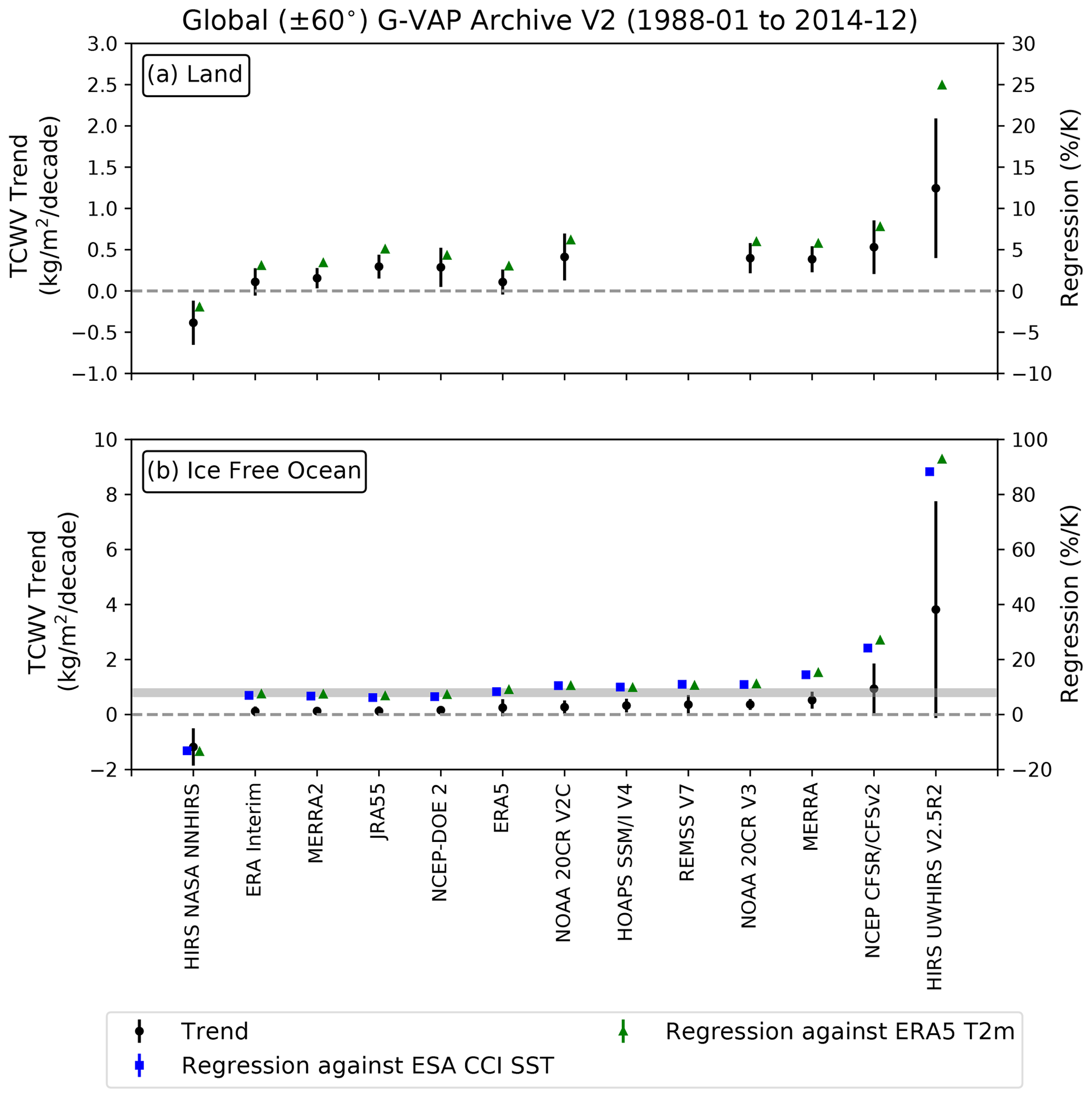
Figure 8Trend estimates in total column water vapour (TCWV) (in kg m−2 per decade) for data records that span the common long period (1988–2014) for global land (a) and ice-free oceans (b) between ±60°. Trends are represented as black dots with the estimated uncertainty of the trend shown in vertical bars. Also shown on the right-hand y axes are the regression coefficient (% K−1) for each data record. Regression has been carried out against sea surface temperature (SST) from the ESA Climate Change Initiative (CCI) and 2 m air temperature from ERA5 (ERA5 T2m). These are shown as blue squares and green triangles, respectively, with the regression error as vertical bars. The grey-shaded region on the bottom panel denotes the expected range of regression values and actual expectation based on the mean change in SST (Wentz and Schabel, 2000).
In addition to these trends, Fig. 8 provides the regression of each TCWV dataset against SST and T2m surface temperature records. We also include the expected theoretical range (as described in Wentz and Schabel, 2000) for ice-free ocean regression coefficients. As with the first phase of G-VAP (Schröder et al., 2019), we see significant differences between the records within the archive. The first noticeable result is that the HIRS records exhibit more extreme behaviours than the other datasets. For NNHIRS, regression against ERA5 T2m yields values of −13.46 ± 1.19 % K−1 over the ocean and −1.96 ± 0.43 % K−1 over land surfaces. Regression against ESA CCI SST over the ocean shows a similar result to ERA5 with a value of −13.17 ± 1.17 % K−1. The UWHIRS product displays the largest regression coefficients with values of 92.81 ± 1.02 and 88.28 ± 1.04 % K−1 over ice-free ocean surfaces (ERA5 T2m, ESA CCI SST, respectively) and 24.94 ± 0.23 % K−1 over land (ERA5 T2m).
For the other products, the main results we observe are the following:
-
For regression coefficients over ice-free oceans, we found ranges of 6.77 ± 0.24 to 27.02 ± 0.51 % K−1 for ERA5 T2m and 6.17 ± 0.24 to 24.17 ± 0.45 % K−1 against ESA CCI SST.
-
Over land surfaces, the range of regression coefficients is between 3.00 ± 0.17 and 7.77 ± 0.16 % K−1 against ERA5.
-
Accounting for the uncertainty in the regression coefficients against ERA5 T2m and ESA CCI SST, we find that ERA-Interim, MERRA2, NCEP-DOE 2 and ERA5 fall within the theoretical range following Clausius–Clapeyron for both temperature datasets. When only taking into account ERA5 T2m, the JRA55 product also falls within this range.
Examination of the spatial distributions of TCWV trends is used to investigate the inter-variability of these global trends further. Figure 9a presents the median absolute deviation (MAD) of long-period trends between the respective archive datasets. From looking at all records in this way, we can see three key features:
-
Sea-ice boundaries show up as large MAD values with high spatial variability at high latitudes.
-
Tropical oceans exhibit high levels of variability.
-
Regions of high variability are observed over South America and central Africa.
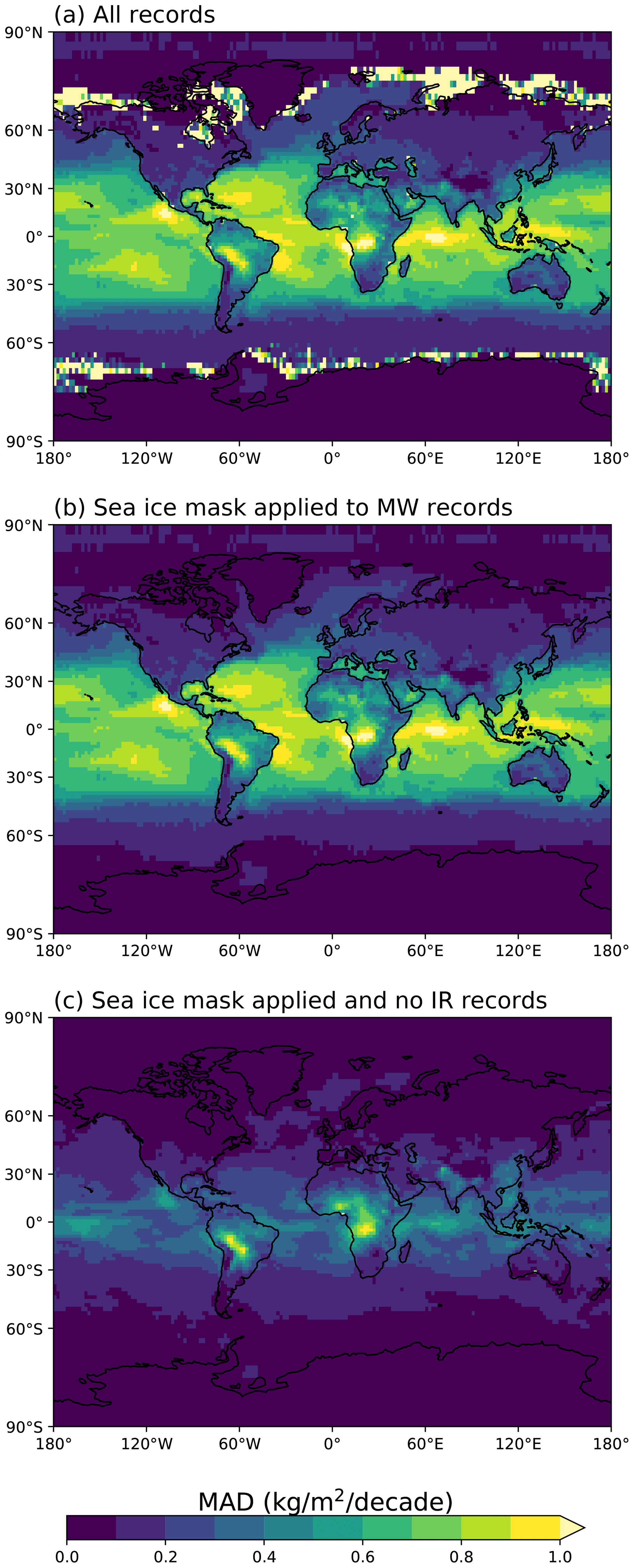
Figure 9Mean absolute deviation (MAD) of archive total column water vapour (TCWV) trend estimates for the period between 1988–2014 (a). High MAD values observed in the tropics are on the order of 25 % of observed trends, while the highest MAD values (> 1.0 kg m−2 per decade) are observed at high latitudes and are related to sea ice. Application of the sea-ice mask (see Fig. 2) to the microwave (MW) records removes these effects seen at high latitudes (b), while the high variability seen in the tropics is related to the infrared-only products (c).
The first feature is easily accounted for by applying the sea-ice mask to the satellite records impacted by sea ice. From Fig. 9b, we can observe that the mask successfully removes the previous noise.
Figure C1 presents the spatial distribution of TCWV trends for the 13 long-term records. The outlier behaviour observed in IR HIRS records is clearly driven by strong positive/negative trends over low stratiform cloud regions between ±40°.
4.2.2 Analysis of breakpoints
A high level of stability is a key requirement in the case that long-term data records are utilised in climate change analysis. Different approaches can be applied to assess stability. Here, the analysis of breakpoints (in kg m−2) at a specific time is carried out. As a first step, as with the trends, the TCWV anomaly time series are computed. Input to the breakpoint analysis is then the anomaly difference to HOAPS v4 over ocean and ERA5 over land (see Sect. 3.4 for details).
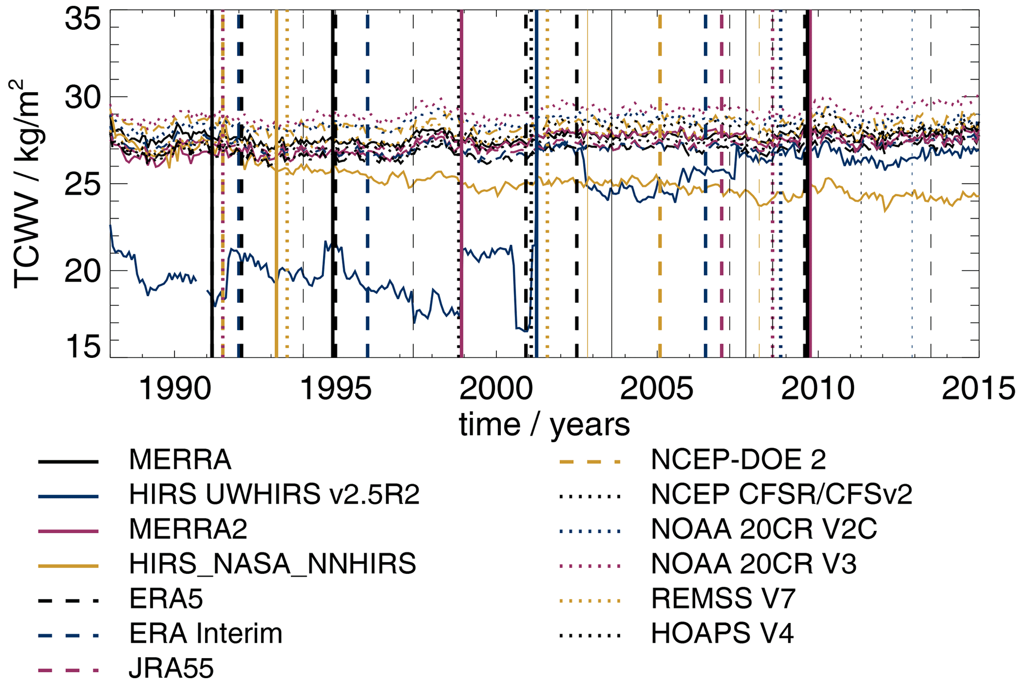
Figure 10Anomaly time series of TCWV, averaged over the global ice-free ocean within 60° N/S, from members of the G-VAP data archive that cover the period 1988–2014. Each average of the TCWV time series was added to each anomaly time series in order to visualise biases between the data records. Vertical lines denote observed breakpoints using the same colour bar as for the anomaly time series. The vertical line is plotted in bold in the case that the PMF and SNH tests both detected the breakpoint.
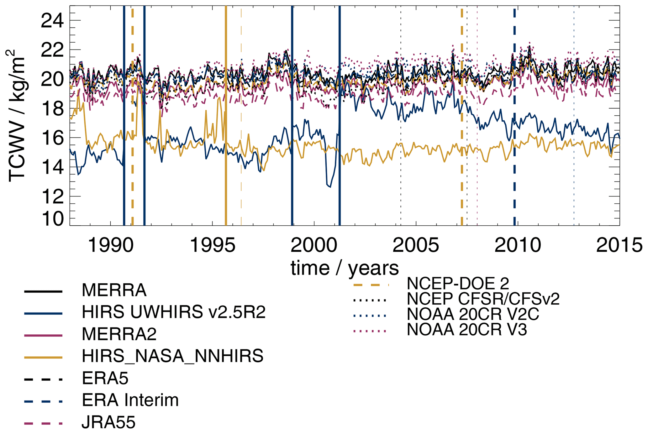
Figures 10 and 11 show the anomaly time series, shifted by the data record's mean value, and breakpoints observed over the ocean and land, respectively. The spread among the data records is approximately 3 kg m−2, with the exception of the two HIRS-based data records. The breakpoint analysis identified 38 breakpoints over the ocean, 21 of which were identified by both homogeneity tests. Over land, we found 13 breakpoints, 9 of which were observed by both tests. Only two out of nine breakpoints observed over land are also present over the ocean when applying a match criterion of ±3 months. It is recalled that the homogeneity analysis is applied unsupervised and consistently to all data records such that the results for the different data records are comparable. The breakpoint analysis might not necessarily identify breakpoints correctly, in terms of their presence and strength, and it might also miss breakpoints. An example of the latter is a seemingly undetected breakpoint in the NNHIRS record over land in late 1989. A possible reason is that breakpoints close to the start and stop times of the data records are difficult to detect. When looking at the anomaly time series, the NNHIRS data record exhibits a decrease in TCWV over ocean until approximately 1998, while TCWV from UWHIRS decreases over land after 2001; both features are in contrast to the other data records. Both seem to be affected by a stability issue, that is, by a change in bias over time. Also noteworthy are anomaly features in the time series of NNHIRS over land in the period 1990–1995.
Table 2Breakpoints detected by the PMF and SNH tests and coincident events. Results are shown for the global ocean. The breakpoints are characterised by the time of the event (yyyy-mm) and their strength (in kg m−2). The strength of the breakpoint is printed in bold if both tests agree on the date within ±3 months. Break events marked with “∗” are taken from Schröder et al. (2019). Information on satellite status was taken from https://www.ospo.noaa.gov/Operations/POES/status.html (last access: 3 March 2022).
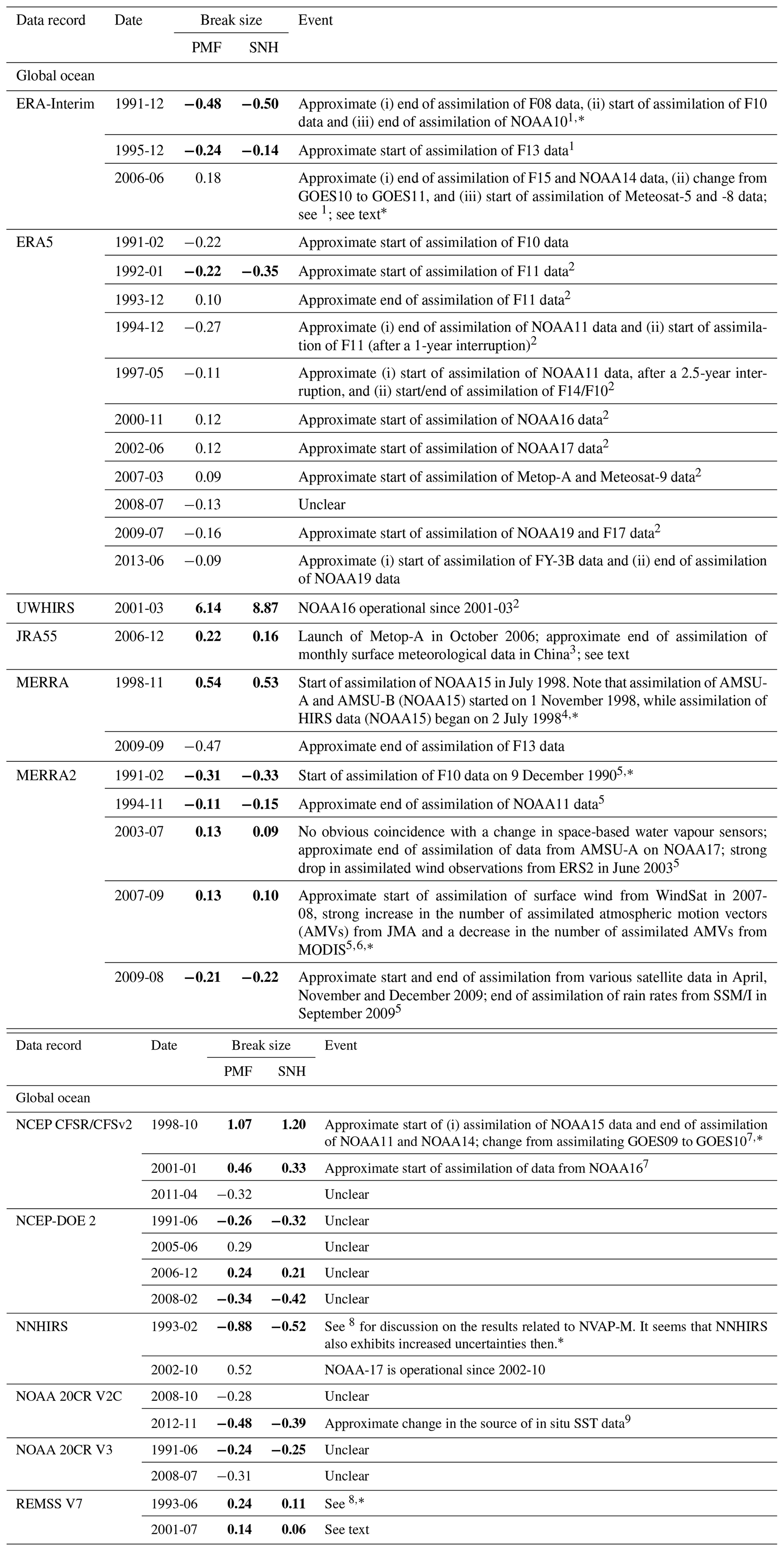
References: 1 Dee et al. (2011); 2 Hersbach et al. (2020); 3 Kobayashi et al. (2015); 4 Rienecker et al. (2011); 5 McCarty et al. (2016); 6 Gelaro et al. (2017); 7 Saha et al. (2010); 8 Schröder et al. (2016); 9 Slivinski et al. (2019).
The time and strength of detected breakpoints are given in Tables 2 and 3, together with a potential explanation for the presence of such breakpoints. It is noted that the given explanations are actually temporally coincident between observed breakpoints and changes in the observing system. However, a physical explanation has not been explored and is thus not provided here. In the majority of cases, the observed breakpoint coincides with a change in the observing system. In 20 % of the cases with confirmed breakpoints, a potential reason for the breakpoint is unknown. The observed breakpoints are generally small, except for the breakpoints observed in UWHIRS. Most breakpoints are observed in ERA5 over the ocean. It is emphasised that the anomaly difference time series between HOAPS v4 and ERA5 exhibits a very low noise level, and only then can the breakpoint analysis detect small breakpoints. However, only one breakpoint of ERA5 was confirmed with the second homogeneity test. In contrast, the strong breakpoints in UWHIRS reduce the ability of the applied methodology to detect additional small breaks, for example, in 2002 over the ocean (see Fig. 10). If a break is caused by the utilised references (HOAPS v4 over ocean and ERA5 over land), such a break would need to be present in most data records. This seems not to be the case. The breakpoint over the ocean between REMSS V7 and HOAPS V4 in July 2001 does not coincide with a change in the observing system. The break coincides with a small increase and anomaly present in most data records. It can be a topic of future G-VAP efforts to analyse this feature further, e.g. by comparing the full SSM/I and SSMIS climatology to a climatology of near-constant Equator crossing times (similarly as in Allan et al., 2022).
Table 3Same as Table 2 but for global land surfaces. For the following data records, no breakpoints were detected over land: JRA55, MERRA, and MERRA2.
References: 1 Dee et al. (2011); 2 Saha et al. (2010).
Finally, the largest and smallest mean trend estimates shown in Fig. 8 are observed for NNHIRS and ERA-Interim (smallest, i.e. negative trends) and UWHIRS and NCEP CFSR/CFSv2. In these cases, the observed breakpoints are either predominantly strongly positive or negative and explain the unexpectedly large and small trend estimates discussed earlier.
4.2.3 Correlation to climate indices
For the final analysis, TCWV anomalies for each long-term record were compared to the seven climate indices detailed in Table B1. An example of NAO, NINO3.4 and PDO correlation maps is shown in Fig. 12, with statistically significant correlations indicated with hatching. Figures for each data record with all seven climate indices can be found in the Supplement. Next, these correlations were inter-compared between the datasets for each climate index. Notably, we identified two region types where at least 50 % and 100 % of the records agreed on either positive or negative correlations. The absolute values differ over land and ocean surfaces as the MW satellite records only provide data over ice-free global oceans. The results from this test are shown in Fig. 13, with negatively correlated regions shown on the left-hand side in orange, while regions of positive correlation are presented on the right-hand side in purple. The key results from these comparisons show the following:
-
Generally, positive correlations between all datasets occur in expected regions (as outlined in Table B1) related to the specific index.
-
We also observe positive correlations between all water vapour records off the coast of Antarctica related to ENSO3.4 and the Southern Ocean and Tropical Warm Pool regions with AMM.
-
Ambiguity in the agreement among data records is also found over Africa for PDO, the Pacific Ocean for NAO, and over the African and Antarctic continents for PMM.
-
Consistent negative correlations with PDO within the archive are observed over northwest America and eastern Europe.
-
Over Greenland and North America, all water vapour records agree on a negative correlation to NAO and AO.
-
However, we observe an ambiguity in negative correlations above 80° N for PMM; the broader Pacific regions for NINO3.4 and PDO; and over Africa, South America, and ocean regions for tropical latitudes for AO and NAO.
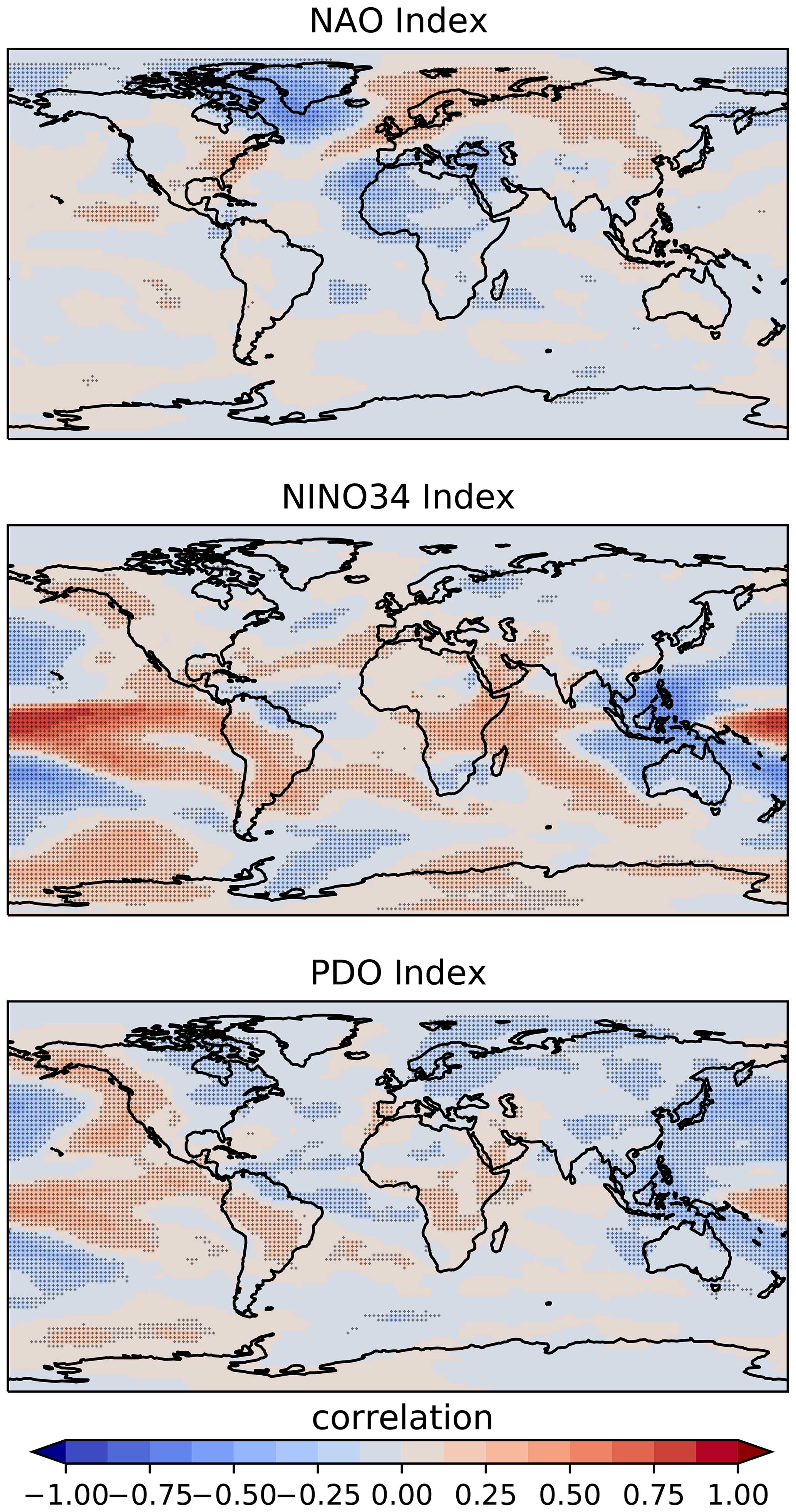
Figure 12Global maps of the correlation between ERA5 total column water vapour (TCWV) and the North Atlantic Oscillation (NAO), El Niño–Southern Oscillation Index 3.4 (NINO3.4), and Pacific Decadal Oscillation (PDO) climate indices. The stippling indicates areas where the correlation is within the 95 % confidence level.
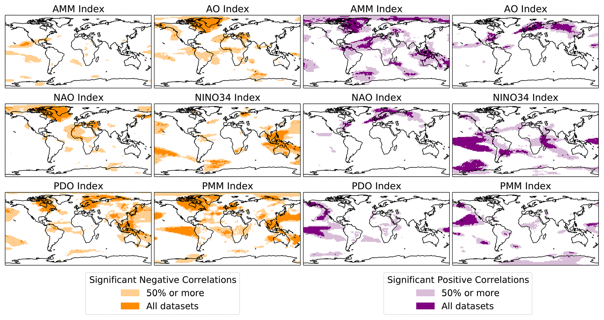
Figure 13Summary of global regions where the water vapour records that cover the long period (1988–2014) significantly correlate with the different climate indices. Negative correlations are shown in orange on the left, and positive correlations are shown in purple on the right. Areas coloured in the lighter shade of colour indicate where at least 50 % of all water vapour datasets show significant correlations, while darker-coloured areas indicate where 100 % of records show significant correlations to the climate indices.
This study continues the G-VAP activities carried out within its first phase. Approaches used here differ from approaches used in the first phase of G-VAP. The archive contains more members, particularly from reanalysis and HIRS; different periods were considered for the common period and long-term analysis; and a new land/sea and sea-ice mask was used. Also, new versions of HOAPS (here: HOAPS V4; in archive version 1: HOAPS V3.2) and ERA (here: ERA5; in archive version 1: ERA-Interim) served as references for breakpoint detection, and different SST (here: SST from ESA CCI, corrected v2; in phase 1: Optimum Interpolation Sea Surface Temperature (OISST) from NOAA, v2) and T2m data records (not at all in phase 1) were employed for regression analysis. All this might provide a reason for differences to results from G-VAP's first phase. Nonetheless, this study generally confirms the results from the first G-VAP phase (Schröder et al., 2016, 2019):
-
The data records exhibit distinct spatial features in terms of biases, standard deviation and mean absolute trend differences. Again, South America and central Africa stick out as well as additional regions: the Sahel, IGP, and parts of China and Japan.
-
Large differences in trend and regression estimates occur over the ocean.
-
Most data records are affected by breakpoints, where some of the physical causes can be identified.
-
The occurrence of breakpoints seems to have a regional dependency (here, ocean versus land), and in most cases, the breakpoints coincide with changes in the observing system.
Exclusion of IR-based products from the ensemble removes these differences and variability significantly, particularly over tropical oceans. This is interpreted to be dominated by the instability of the underlying HIRS data records.
The number of data records that exhibit regression values within the expected range over ocean is larger among data records from the G-VAP data archive version 2 than from the G-VAP data archive version 1. This can likely be explained by the archive version 2 containing mainly additional reanalysis data records. It is recalled that the relationship between TCWV and surface temperature is affected by advection, precipitation, and other small-scale and regional events, which impact equilibrium between surface and atmosphere. Also, surface temperature and TCWV instead of near-surface air temperature and mixing ratio are considered here (e.g. Mieruch et al., 2014). Violations of these assumptions can give reasons for larger-than-expected regression values (Trenberth et al., 2005). Additionally, Shi et al. (2018) observed an ocean-basin-dependent time lag between SST and TCWV. Results shown in Wentz and Schabel (2000) indicate that the lag can also be a function of event. Even more so, the local response to ENSO also exhibits variability, as observed by Stephens et al. (2018) for precipitation. The presence of time lags between SST and TCWV during El Niño events was not considered during computation of regressions. Following discussions in Falk et al. (2022) on land areas, the relation between air temperature and surface temperature is complex, and locally the difference between air and surface temperature reaches a few kelvin. This depends on various factors, such as local time, cloudiness and surface type (e.g. Good, 2016; Rayner et al., 2020). Additionally, the expectation over land is affected by the potential limitation of water vapour fluxes into the atmosphere (Byrne and O'Gorman, 2016). The input flux depends on various processes and parameters, e.g. advection from ocean to land, presence of surface water, soil moisture and other factors. Byrne and O'Gorman (2016) conclude that the moisture transport from the ocean is the dominating process for changes in specific humidity over land, and evapotranspiration processes cause changes in RH over land. The presence of increased SST and TCWV over the ocean during El Niño events might lead to a larger transport of moisture from ocean to land. At the same time, increased surface temperature might not be present over land and can thus lead to a reduced correlation between land surface temperature and TCWV.
Looking at the differences between individual data records to the ensemble mean reveals that the data records that rely on retrievals predominantly applicable to clear-sky conditions exhibit biases to the ensemble mean over the ITCZ and storm tracks; that is, the bias coincides with predominantly cloudy regions.
The retrievals of TCWV are based on measurements obtained in different parts of the electromagnetic spectrum: among others, the visible, the near-infrared (NIR), infrared (IR) and microwave frequencies. Except for microwave observations, all related retrievals are predominantly applied under clear-sky conditions. Though instantaneous water vapour products can show high quality and low uncertainty, this is not necessarily true for the gridded and temporally averaged products: conditions in clouds are typically more humid than the surrounding clear-sky areas (e.g. Fetzer et al., 2006) and are not taken into account by the retrieval's clear-sky observations. This causes a so-called clear-sky bias (CSB) that is on the order of 10 % (Sohn and Bennartz, 2008). Also, TCWV retrieved from observations in the visible and NIR rely on reflected solar radiation and, thus, is only available during daytime (affected products are CM SAF/WV_cci over land, GOME Evolution, MODIS (NIR) and MPIC OMI). Additionally, most satellite-based TCWV CDRs (climate data records) rely on measurements from polar-orbiting satellites. Thus, observations of TCWV are only available at specific times of the day, and the full day is not covered with samples. The following data records rely on single sensor observations only, with the Equator crossing time given in brackets: AIRS v6/V7 (10:30 + 13:30), AIRWAVE v2 (10, 10:30), CM SAF/WV_cci (10:30, over land), EMiR (10, 10:30), GOME Evolution (10, 10:30), MODIS Terra (10:30), MODIS Aqua (13:30) and MPIC OMI (13:40). All other satellite-based data records sample more frequently but at different times and frequencies, partly affected by orbital drift and partly varying in time. Details on satellite Equator crossing times can be found at https://space.oscar.wmo.int/satellites (last access: 8 November 2023). Examples of Equator crossing times affected by orbital drift can be found at https://www.star.nesdis.noaa.gov/smcd/emb/vci/VH/vh_avhrr_ect.php (last access: 8 November 2023) and https://www.remss.com/support/crossing-times/ (last access: 8 November 2023). This specific sampling might cause a diurnal cycle sampling bias.
Falk et al. (2022) utilised ERA5 data to assess the joint bias caused by the clear-sky nature of retrievals and the lack of full-day coverage. The basic approach was to compare full-day, all-sky averages with clear-sky averages at specific time slots using ERA5 output. Here their results are briefly summarised as follows: the overall average CSB is approximately −0.9 kg m−2. The CSB is generally negative, with the largest negative values in the ITCZ and storm track regions. Regions with positive areas were observed over stratocumulus regions and Antarctica. Given the dependency on clouds and, among others, the movement of the ITCZ, the spatial distribution of the CSB is a function of season. An example comparison of the CSB at 10:00 LT and the CSB using the full diurnal information from ERA5 exhibits fairly similar results and mainly a noisier appearance. However, as shown for South America and over the full course of the day by Falk et al. (2022), a dependency on local time can be present at a regional scale. It is noted that the effect of orbital drift, of potential changes in diurnal cycles of TCWV and clouds, and of potential changes in spatial cloud distributions with climate change have not been considered here. To some extent, the sign and the spatial features observed in Fig. 7 for AIRWAVE, NNHIRS, UWHIRS and MODIS Terra IR agree with the features from Falk et al. (2022). This is also valid over the ocean for the other MODIS products. Thus, the predominant clear-sky sampling nature of these products might at least partly explain the observed features. However, the overall bias for AIRS (except over tropical South America) and CM SAF/WV_cci (except over central eastern China, though potentially related to uncertainties arising from the treatment of aerosols) is fairly small, while GOME Evolution (land and ocean), MPIC OMI (land and ocean), MODIS TERRA+AQUA NIR (land) and MODIS AQUA IR (land) exhibit positive biases, in contrast to the expectation. It is noted that the ensemble is dominated by all-sky data records from reanalysis and microwave observations. Nonetheless, the ensemble mean has members from visible, NIR and IR observations as well and, even more so, contains a mixture of information and uncertainty.
We introduce a new version of the G-VAP data archive. It features new versions and newly added data records, while some are superseded or removed from the archive. The main change to the previous version is the extended temporal coverage from 1979–2019 and that the individual temporal coverage of the data records is kept. A flag was added to easily identify periods in which no data are available. Based on the updated G-VAP data archive, various analyses were carried out to characterise the individual data records, with a focus on their fitness to allow for climate analysis. These include the analysis of trends, breakpoints and climate variability. Overall results confirm previously achieved results in G-VAP (see Schröder et al., 2016, 2019), though with differences in the details that can be expected given changes in the methodology. New results include the following: the intercomparison effort has been extended by analysing standard deviation, coefficient of variation, and range between ensemble minimum and maximum. Associated results emphasise the large variability between data records over the poles, South East Asia and dry atmospheres in general. This suggests that despite the efforts of, for example, Crewell et al. (2021), dedicated regional quality analyses of water vapour records are still needed. In the area of climate variability, the ENSO contribution to the TCWV variability is largely consistent in terms of spatial patterns between the data records. However, it exhibits considerable variability in strength. The analysis for large-scale regions and phase shifts per event indicates the presence of teleconnections. These results warrant further investigation, and the scope would fit within a dedicated GEWEX process evaluation study (PROES). In the assessment of biases, analysis of the clear-sky bias and to some extent of the diurnal sampling bias confirms previous conclusions that such biases significantly impact predominantly sampled clear-sky TCWV products if aggregated in space or time. Nonetheless, associated uncertainty estimation, additional analysis on potential all-sky versus cloudy-sky observations, sampling impacts from orbital drift, and climate change impacts on dependent variables such as clouds and their diurnal cycle are still broad fields for additional scientific analysis. Finally, a careful improvement of the temporal stability of HIRS TCWV data records would be highly beneficial, given that HIRS offers a unique opportunity to retrieve TCWV over land and ocean beginning in the late 1970s.
| Abbreviation | Definition |
| AIRS | Atmospheric Infrared Sounder |
| AIRWAVE | Advanced InfraRed WAter Vapour Estimator |
| AMSR2 | Advanced Microwave Scanning Radiometer 2 |
| AMSR-E | Advanced Microwave Scanning Radiometer for EOS |
| AMIP | Atmospheric Model Intercomparison Project |
| AR6 | Sixth Assessment Report |
| ATOVS | Advanced TIROS Operational Vertical Sounder |
| CFSR | Climate Forecast System Reanalysis |
| CFSv2 | Coupled Forecast System model Version 2 |
| CM SAF | Satellite Application Facility on Climate Monitoring |
| ECMWF | European Centre for Medium-Range Weather Forecasts |
| ENSO | El Niño–Southern Oscillation |
| EMiR | ERS/Envisat MWR Recalibration and Water Vapour TDR Generation |
| ERA-Interim | ECMWF interim reanalysis |
| ERA-20C | ECMWF Reanalysis of the 20th Century |
| ERA5 | ECMWF Reanalysis v5 |
| ESA | European Space Agency |
| EUMETSAT | European Organisation for the Exploitation of Meteorological Satellites |
| GDAP | GEWEX Data and Assessments Panel |
| GEWEX | Global Energy and Water cycle Exchanges |
| GOME/GOME-2 | Global Ozone Monitoring Experiment |
| GOME EVOL | GOME Evolution |
| G-VAP | GEWEX Water Vapor Assessment |
| HIRS | High-resolution Infrared Radiation Sounder |
| HOAPS | Hamburg Ocean Atmosphere Parameters and Fluxes from Satellite data |
| JAXA | Japan Aerospace Exploration Agency |
| JMA | Japan Meteorological Agency |
| JRA-55 | Japanese 55-year Reanalysis |
| MAD | Median absolute deviation |
| MERIS | MEdium Resolution Imaging Spectrometer |
| MERRA | Modern-Era Retrospective analysis for Research and Applications |
| MERRA-2 | MERRA Version 2 |
| MODIS | Moderate Resolution Imaging Spectroradiometer |
| MPIC | Max Planck Institute for Chemistry |
| MW | Microwave |
| NASA | National Aeronautics and Space Administration |
| NCEP | National Centers for Environmental Prediction |
| NIR | Near-infrared |
| NNHIRS | Neural Network High-resolution Infrared Radiation Sounder |
| Abbreviation | Definition |
| NOAA | National Oceanic and Atmospheric Administration |
| NVAP | NASA Water Vapor Project |
| NVAP-M | NVAP – Making Earth Science Data Records for Research Environments |
| OLCI | Ocean and Land Colour Instrument |
| OMI | Ozone Monitoring Instrument |
| PAOBS | paid observations |
| PROES | GEWEX process evaluation studies |
| REMSS | Remote Sensing Systems |
| SCIAMACHY | SCanning Imaging Absorption spectroMeter for Atmospheric CHartographY |
| SSM/I | Special Sensor Microwave Imager |
| SSMIS | Special Sensor Microwave Imager/Sounder |
| TCWV | total column water vapour |
| TIROS | Television Infrared Observation Satellite |
| TMI | TRMM Microwave Imager (Tropical Rainfall Measuring Mission) |
| UWHIRS | University of Wisconsin High-resolution Infrared Radiation Sounder (V2.5R2) |
| WCRP | World Climate Research Programme |
| WV_cci | Water Vapour Climate Change Initiative |
Further details on climate indices used in this study are presented here in Table B1.
Chiang and Vimont (2004)Thompson and Wallace (1998)Walker (1924)Rogers (1984)Barnston and Livezey (1987)Hurrell (1995)Walker (1924)Rasmusson and Carpenter (1982)Mantua et al. (1997)Zhang et al. (1997)Chiang and Vimont (2004)
The spatial patterns of global trends calculated for each record that covers the long analysis period are shown here in Fig. C1.
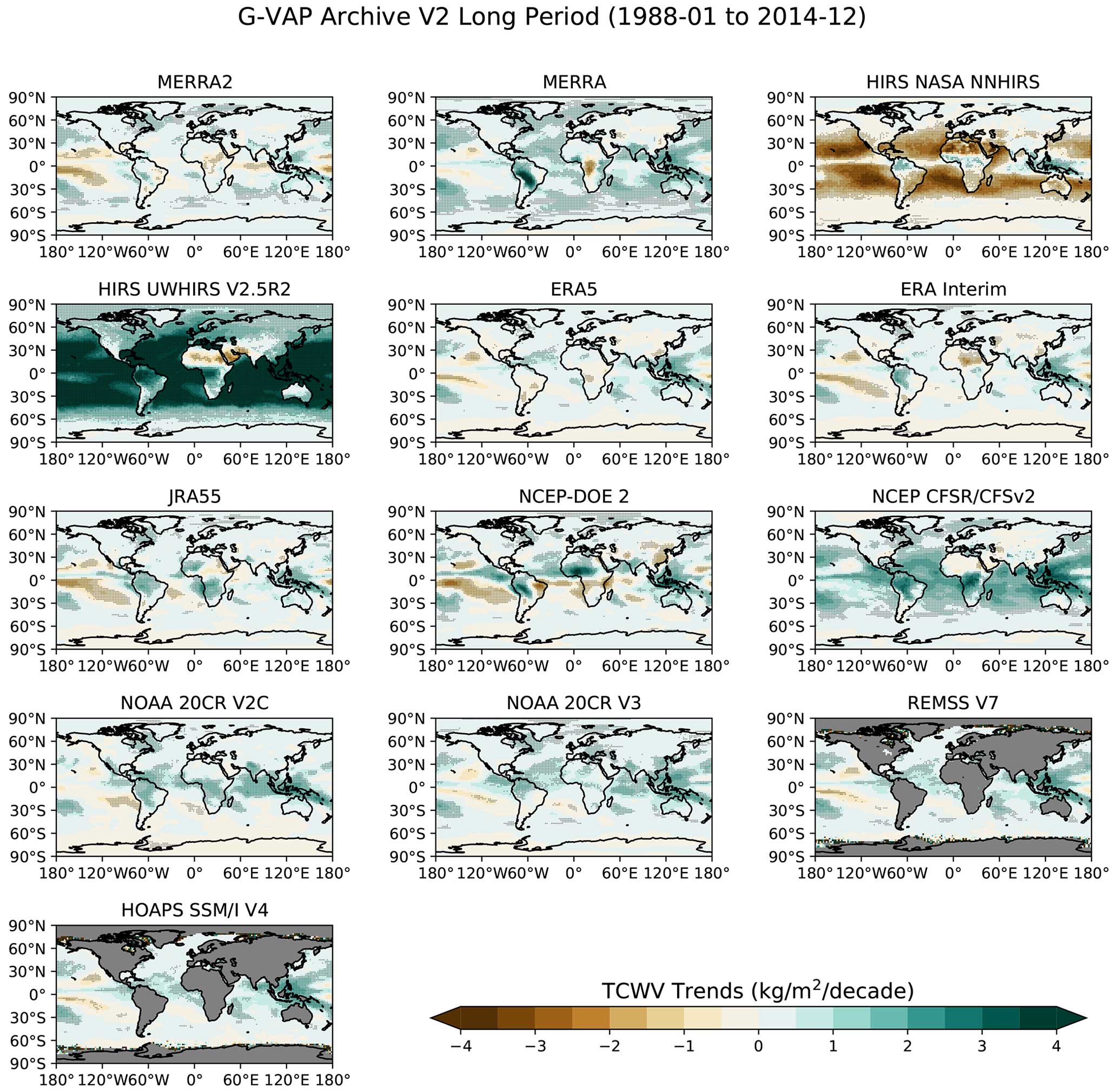
Figure C1Global maps of total column water vapour (TCWV) trend estimates from all records between 1988 and 2014. Regions where trends were not statistically significant are highlighted with stippling. These regions tend to coincide with stronger trends; however, it should be noted that the reported trends by G-VAP are used to identify issues rather than an analysis of climate change. Therefore, it is more likely these areas experience higher ranges of variability, which introduces noise into the calculation (Weatherhead et al., 1998) Thus, longer time series are required to improve confidence in reported trends.
Version 1 of the G-VAP data archive was generated in April 2017. The data are available in netCDF format and can be accessed via https://doi.org/10.5676/EUM_SAF_CM/GVAP/V001 (Schröder et al., 2017b). The AIRWAVEv2 data (Castelli et al., 2019) are available on request from Elisa Castelli (e.castelli@isac.cnr.it) and Enzo Papandrea (e.papandrea@isac.cnr.it). Aqua/AIRS L3 Monthly Standard Physical Retrieval (AIRS+AMSU) 1 degree x 1 degree V6.0 and V7.0 can be freely accessed via the Goddard Earth Sciences Data and Information Services Center (GES DISC, https://doi.org/10.5067/KUC55JEVO1SR, AIRS project, 2019). The CM SAF/WV_cci COMBI product can be freely accessed from https://doi.org/10.5676/EUM_SAF_CM/COMBI/V001 (Schröder et al., 2023). The GOME EVOL product can be accessed from https://doi.org/10.1594/WDCC/GOME-EVL_water_vapor_clim_v2.2 in netCDF format (Beirle et al., 2018b). ERA5 data can be freely accessed from the Copernicus Climate Data Store (https://doi.org/10.24381/cds.f17050d7, Hersbach et al., 2023). MODIS MOD08_M3 (https://doi.org/10.5067/MODIS/MOD08_M3.061, Platnick et al., 2015b) and MYD08_M3 (https://doi.org/10.5067/MODIS/MYD08_M3.061, Platnick et al., 2015a) products can be freely accessed from NASA's level-1 and Atmospheric Archive & Distribution System (LAADS). The MPICOMI TCWV climate data record is available from https://doi.org/10.5281/zenodo.7973889 (Borger et al., 2023b). The NCEP-DOE 2 reanalysis is freely available from https://psl.noaa.gov/data/gridded/data.ncep.reanalysis2.html (Physical Sciences Laboratory, 2021; Kanamitsu et al., 2002). Version 2c of NOAA's 20th century reanalysis (NOAA 20CR V2c) is freely available from https://psl.noaa.gov/data/gridded/data.20thC_ReanV2c.html (Physical Sciences Laboratory, 2020a; Compo et al., 2011), version 3 of NOAA20 CR is also freely available from https://www.psl.noaa.gov/data/gridded/data.20thC_ReanV3.html (Physical Sciences Laboratory, 2020b; Slivinski et al., 2019).
The supplement related to this article is available online at: https://doi.org/10.5194/acp-24-9667-2024-supplement.
TT and MS collected the original TCWV data records used in version 2 of the G-VAP archive. TT processed all records as per the common grid format described in this study. TT and MS analysed all the records within the archive and generated results. TT and MS wrote the first draft of the paper, with all authors contributing to the discussion and interpretations of results as well as manuscript revisions. Data record principal investigators provided expert advice on interpretation of breakpoint analysis.
The contact author has declared that none of the authors has any competing interests.
Publisher's note: Copernicus Publications remains neutral with regard to jurisdictional claims made in the text, published maps, institutional affiliations, or any other geographical representation in this paper. While Copernicus Publications makes every effort to include appropriate place names, the final responsibility lies with the authors.
This article is part of the special issue “Analysis of atmospheric water vapour observations and their uncertainties for climate applications (ACP/AMT/ESSD/HESS inter-journal SI)”. It is not associated with a conference.
Tim Trent acknowledges the support of ESA (contract no. 4000131292) via the Living Planet Fellowship programme. Marc Schröder acknowledges the support of the EUMETSAT member states through the Satellite Application Facility on Climate Monitoring (CM SAF). Ulrike Falk acknowledges the support of ESA (contract no. 4000123554) via the Water_Vapour_cci project of ESA's Climate Change Initiative (CCI). The AIRWAVEv2 work has been performed under the ESA-ESRIN (contract no. 4000108531/13/I-NB). Support for the Twentieth Century Reanalysis project is provided by the US Department of Energy, Office of Science Biological and Environmental Research (BER), by the National Oceanic and Atmospheric Administration Climate Program Office, and by the NOAA Physical Sciences Laboratory. Gilbert P. Compo acknowledges the support of the NOAA Physical Sciences Laboratory through the NOAA Cooperative Agreement with CIRES (NA17OAR4320101). The AIRS project work was carried out at the Jet Propulsion Laboratory, California Institute of Technology, under a contract with the National Aeronautics and Space Administration (80NM0018D0004). Johannes K. Nielsen acknowledges the support of the EUMETSAT member states through the Radio Occultation Meteorology Satellite Application Facility. The EMiR data record was created under ESA (contract no. 4000109537/13/I-AM). The NVAP-M data record was supported by NASA MEaSUREs (contract MEAS-06-0023). The MODIS IR TPW products have been developed at the Space Science and Engineering Center, University of Wisconsin–Madison, funded by NASA (grant number NNX14AN48G). The UWHIRS data record was created under NOAA (contract no. NA15NES4320001). All authors would like to thank Eric Fetzer, Richard Allan and the anonymous reviewer whose comments and suggestions helped improve the final paper. This research used the ALICE high-performance computing facility at the University of Leicester.
This research has been supported by the Natural Environment Research Council (grant no. PR140015) and the European Space Agency (grant no. 4000131292).
This paper was edited by Matthew Lebsock and reviewed by Eric Fetzer and one anonymous referee.
AIRS project: Aqua/AIRS L3 Monthly Standard Physical Retrieval (AIRS+AMSU) 1 degree x 1 degree V7.0, Goddard Earth Sciences Data and Information Services Center (GES DISC), Greenbelt, MD, USA [data set], https://doi.org/10.5067/KUC55JEVO1SR, 2019. a, b
AIRS Science Team and Teixeira, J.: AIRS/Aqua L3 Monthly Standard Physical Retrieval (AIRS+AMSU) 1 degree x 1 degree V006, Greenbelt, MD, USA, Goddard Earth Sciences Data and Information Services Center (GES DISC) [data set], https://doi.org/10.5067/Aqua/AIRS/DATA319, 2013. a
Alexandersson, H.: A homogeneity test applied to precipitation data, J. Climatol., 6, 661–675, 1986. a
Allan, R. P., Willett, K. M., John, V. O., and Trent, T.: Global changes in water vapor 1979–2020, J. Geophys. Res.-Atmos., 127, e2022JD036728, https://doi.org/10.1029/2022JD036728, 2022. a, b
Andersson, A., Fennig, K., Klepp, C., Bakan, S., Graßl, H., and Schulz, J.: The Hamburg Ocean Atmosphere Parameters and Fluxes from Satellite Data – HOAPS-3, Earth Syst. Sci. Data, 2, 215–234, https://doi.org/10.5194/essd-2-215-2010, 2010. a
Andersson, A., Graw, K., Schröder, M., Fennig, K., Liman, J., Bakan, S., Hollmann, R., and Klepp, C.: Hamburg Ocean Atmosphere Parameters and Fluxes from Satellite Data – HOAPS 4.0, Satellite Application Facility on Climate Monitoring (CM SAF), https://doi.org/10.5676/EUM_SAF_CM/HOAPS/V002, 2017. a
Barnston, A. G. and Livezey, R. E.: Classification, seasonality and persistence of low-frequency atmospheric circulation patterns, Mon. Weather Rev., 115, 1083–1126, 1987. a
Beirle, S., Lampel, J., Wang, Y., Mies, K., Dörner, S., Grossi, M., Loyola, D., Dehn, A., Danielczok, A., Schröder, M., and Wagner, T.: The ESA GOME-Evolution “Climate” water vapor product: a homogenized time series of H2O columns from GOME, SCIAMACHY, and GOME-2, Earth Syst. Sci. Data, 10, 449–468, https://doi.org/10.5194/essd-10-449-2018, 2018a. a, b
Beirle, S., Lampel, J., Wang, Y., Wagner, T., Grossi, M., and Loyola, D.: The GOME-Evolution total column water vapor “climate” product (Version 2.2), World Data Center for Climate (WDCC) at DKRZ [data set], https://doi.org/10.1594/WDCC/GOME-EVL_water_vapor_clim_v2.2, 2018b. a, b
Borbas, E. E., Seeman, S. W., Kern, A., Moy, A., Li, L., Gumley, L., and Menzel, W. P.: MODIS atmospheric profile retrieval algorithm theoretical basis document, Version 6, Cooperative Institute for Meteorological Satellite Studies, University of Wisconsin-Madison, Madison, WI, https://modis-images.gsfc.nasa.gov/_docs/MOD07_atbd_v7_April2011.pdf (last access: 23 November 2023), 2011. a
Borger, C., Beirle, S., Dörner, S., Sihler, H., and Wagner, T.: Total column water vapour retrieval from S-5P/TROPOMI in the visible blue spectral range, Atmos. Meas. Tech., 13, 2751–2783, https://doi.org/10.5194/amt-13-2751-2020, 2020. a
Borger, C., Beirle, S., and Wagner, T.: A 16-year global climate data record of total column water vapour generated from OMI observations in the visible blue spectral range, Earth Syst. Sci. Data, 15, 3023–3049, https://doi.org/10.5194/essd-15-3023-2023, 2023a. a, b
Borger, C., Beirle, S., and Wagner, T.: MPIC OMI Total Column Water Vapour (TCWV) Climate Data Record, Zenodo [data set], https://doi.org/10.5281/zenodo.7973889, 2023b. a, b
Bove, M. C., Elsner, J. B., Landsea, C. W., Niu, X., and O'Brien, J. J.: Effect of El Niño on US landfalling hurricanes, revisited, B. Am. Meteorol. Soc., 79, 2477–2482, 1998. a
Byrne, M. P. and O'Gorman, P. A.: Understanding decreases in land relative humidity with global warming: Conceptual model and GCM simulations, J. Climate, 29, 9045–9061, 2016. a, b
Castelli, E., Papandrea, E., Di Roma, A., Dinelli, B. M., Casadio, S., and Bojkov, B.: The Advanced Infra-Red WAter Vapour Estimator (AIRWAVE) version 2: algorithm evolution, dataset description and performance improvements, Atmos. Meas. Tech., 12, 371–388, https://doi.org/10.5194/amt-12-371-2019, 2019. a, b
Chiang, J. C. and Vimont, D. J.: Analogous Pacific and Atlantic meridional modes of tropical atmosphere–ocean variability, J. Climate, 17, 4143–4158, 2004. a, b
Chung, E.-S., Soden, B., Sohn, B., and Shi, L.: Upper-tropospheric moistening in response to anthropogenic warming, P. Natl. Acad. Sci. USA, 111, 11636–11641, 2014. a
Colman, R. and Soden, B. J.: Water vapor and lapse rate feedbacks in the climate system, Rev. Mod. Phys., 93, 045002, https://doi.org/10.1103/RevModPhys.93.045002, 2021. a
Compo, G. P., Whitaker, J. S., Sardeshmukh, P. D., Matsui, N., Allan, R. J., Yin, X., Gleason, B. E., Vose, R. S., Rutledge, G., Bessemoulin, P., Brönnimann, S., Brunet, M., Crouthamel, R. I., Grant, A. N., Groisman, P. Y., Jones, P. D., Kruk, M. C., Kruger, A. C., Marshall, G. J., Maugeri, M., Mok, H. Y., Nordli, Ø., Ross, T. F., Trigo, R. M., Wang, X. L., Woodruff, S. D., and Worle, S. J.: The twentieth century reanalysis project, Q. J. Roy. Meteor. Soc., 137, 1–28, 2011. a, b, c
Crewell, S., Ebell, K., Konjari, P., Mech, M., Nomokonova, T., Radovan, A., Strack, D., Triana-Gómez, A. M., Noël, S., Scarlat, R., Spreen, G., Maturilli, M., Rinke, A., Gorodetskaya, I., Viceto, C., August, T., and Schröder, M.: A systematic assessment of water vapor products in the Arctic: from instantaneous measurements to monthly means, Atmos. Meas. Tech., 14, 4829–4856, https://doi.org/10.5194/amt-14-4829-2021, 2021. a
Dee, D. P., Uppala, S. M., Simmons, A. J., Berrisford, P., Poli, P., Kobayashi, S., Andrae, U., Balmaseda, M. A., Balsamo, G., Bauer, P., Bechtold, P., Bechtold, P., Bechtold, P., Bidlot, J., Bormann, N., Delsol, C., Dragani, R., Fuentes, M., Geer, A. J., Haimberger, L., Healy, S. B., Hersbach, H., Hólm, E. V., Isaksen, L., Kållberg, P., Köhler, M., Matricardi, M., McNally, A. P., Monge-Sanz, B. M., Morcrette, J., Park, B., Peubey, C., de Rosnay, P., Tavolato, C., Thépau, J., and Vitart, F.: The ERA-Interim reanalysis: Configuration and performance of the data assimilation system, Q. J. Roy. Meteor. Soc., 137, 553–597, 2011. a, b
Dessler, A. E. and Davis, S.: Trends in tropospheric humidity from reanalysis systems, J. Geophys. Res.-Atmos., 115, D19127, https://doi.org/10.1029/2010JD014192, 2010. a
Diedrich, H., Preusker, R., Lindstrot, R., and Fischer, J.: Retrieval of daytime total columnar water vapour from MODIS measurements over land surfaces, Atmos. Meas. Tech., 8, 823–836, https://doi.org/10.5194/amt-8-823-2015, 2015. a
Douville, H., Raghavan, K., Renwick, J., Allan, R. P., Arias, P. A., Barlow, M., Cerezo-Mota, R., Cherchi, A., Gan, T. Y., Gergis, J., Jiang, D., Khan, A., Pokam Mba, W., Rosenfeld, D., Tierney, J., and Zolina, O.: Water Cycle Changes, in: Climate Change 2021: The Physical Science Basis. Contribution of Working Group I to the Sixth Assessment Report of the Intergovernmental Panel on Climate Change, edited by: Masson-Delmotte, V., Zhai, P., Pirani, A., Connors, S. L., Péan, C., Berger, S., Caud, N., Chen, Y., Goldfarb, L., Gomis, M. I., Huang, M., Leitzell, K., Lonnoy, E., Matthews, J. B. R., Maycock, T. K., Waterfield, T., Yelekçi, O., Yu, R., and Zhou, B., Cambridge University Press, Cambridge, United Kingdom and New York, NY, USA, 1055–1210, https://doi.org/10.1017/9781009157896.010, 2021. a, b
Falk, U., Schröder, M., Brogniez, H., Eiras-Barca, J., Gimeno, L., He, J., Hubert, D., Lambert, J.-C., Preusker, R., Trent, T., and Hegglin, M.: Climate Assessment Report (CAR), Tech. rep., European Space Agency, https://climate.esa.int/documents/1860/Water_Vapour_cci_D5.1_CAR_v3.1.pdf (last access: 24 November 2023), 2022. a, b, c, d
Fennig, K., Schröder, M., Andersson, A., and Hollmann, R.: A Fundamental Climate Data Record of SMMR, SSM/I, and SSMIS brightness temperatures, Earth Syst. Sci. Data, 12, 647–681, https://doi.org/10.5194/essd-12-647-2020, 2020. a, b
Fetzer, E. J., Lambrigtsen, B. H., Eldering, A., Aumann, H. H., and Chahine, M. T.: Biases in total precipitable water vapor climatologies from Atmospheric Infrared Sounder and Advanced Microwave Scanning Radiometer, J. Geophys. Res.-Atmos., 111, D09S16, https://doi.org/10.1029/2005JD006598, 2006. a, b
Fischer, J., Preusker, R., Schröder, M., and Danne, O.: Algorithm Theoretical Baseline Document – Part 1 (ATBD), Tech. rep., European Space Agency, https://climate.esa.int/documents/1336/Water_Vapour_cci_D2.2_ATBD_Part_1_-_MERIS-MODIS-OLCI_L2_products_v2.1.pdf (last access: 24 November 2023), 2021. a
Forster, P., Storelvmo, T., Armour, K., Collins, W., Dufresne, J.-L., Frame, D., Lunt, D. J., Mauritsen, T., Palmer, M. D., Watanabe, M., Wild, M., and Zhang, H.: Chapter 7: the earth's energy budget, climate feedbacks, and climate sensitivity Climate Change 2021: The Physical Science Basis, Contribution of Working Group I to the Sixth Assessment Report of the Intergovernmental Panel on Climate Change, edited by: editors: Masson-Delmotte, V., Zhai, P., Pirani, A., Connors, S. L., Péan, C., Berger, S., Caud, N., Chen, Y., Goldfarb, L., Gomis, M. I., Huang, M., Leitzell, K., Lonnoy, E., Matthews, J. B. R., Maycock, T. K., Waterfield, T., Yelekçi, O., Yu, R., and Zhou, B., Cambridge University Press, https://doi.org/10.1017/9781009157896.009, 2021. a, b
Fowler, H. J., Ali, H., Allan, R. P., Ban, N., Barbero, R., Berg, P., Blenkinsop, S., Senol Cabi, N., Chan, S., Dale, M., Ekström, M., Evans, J. P., Fosser, G., Golding, B., Guerreiro, S. B., Hegerl, G. C., Kahraman, A., Kendon, E. J., Lenderink, G., Lewis, E., Li, X., O'Gorman, P. A., Peat, K. L., Prein, A. F., Pritchard, D., Schär, C., Sharma, A., Stott, P. A., Villalobos-Herrera, R., Villarini, G., Wasko, C., Wehner, M. F., Westra, S., and Whitford, A.: Towards advancing scientific knowledge of climate change impacts on short-duration rainfall extremes, Philos. T. Roy. Soc. A, 379, 20190542, https://doi.org/10.1098/rsta.2019.0542, 2021. a
Gelaro, R., McCarty, W., Suárez, M. J., Todling, R., Molod, A., Takacs, L., Randles, C. A., Darmenov, A., Bosilovich, M. G., Reichle, R., Wargan, K., Coy, L., Cullather, R., Draper, C., Akella, S., Buchard, V., Conaty, A., Conaty, A., Gu, W., Kim, G., Koster, R., Lucchesi, R., Merkova, D., Eric Nielsen, J., Partyka, G., Pawson, S., Putman, W., Rienecker, M., Schubert, S. D., Sienkiewicz, M., and Zhao, B.: The modern-era retrospective analysis for research and applications, version 2 (MERRA-2), J. Climate, 30, 5419–5454, 2017. a
Good, E. J.: An in situ-based analysis of the relationship between land surface “skin” and screen-level air temperatures, J. Geophys. Res.-Atmos., 121, 8801–8819, 2016. a
Hawkins, D. M.: Testing a sequence of observations for a shift in location, J. Am. Stat. Assoc., 72, 180—-186, 1977. a
Held, I. M. and Soden, B. J.: Water vapor feedback and global warming, Annu. Rev. Energ. Env., 25, 441–475, 2000. a
Hersbach, H., Bell, B., Berrisford, P., Hirahara, S., Horányi, A., Muñoz-Sabater, J., Nicolas, J., Peubey, C., Radu, R., Schepers, D., Simmons, A., Soci, C., Abdalla, S., Abellan, X., Balsamo, G., Bechtold, P., Biavati, G., Bidlot, J., Bonavita, M., De Chiara, G., Dahlgren, P., Dee, D., Diamantakis, M., Dragani, R., Flemming, J., Forbes, R., Fuentes, M., Geer, A., Haimberger, L., Healy, S., Hogan, R. J., Hólm, E., Janisková, M., Keeley, S., Laloyaux, P., Lopez, P., Lupu, C., Radnoti, G., de Rosnay, P., Rozum, I., Vamborg, F., Villaume, S., and Thépaut, J.: The ERA5 global reanalysis, Q. J. Roy. Meteor. Soc., 146, 1999–2049, 2020. a, b, c, d
Hersbach, H., Bell, B., Berrisford, P., Biavati, G., Horányi, A., Muñoz Sabater, J., Nicolas, J., Peubey, C., Radu, R., Rozum, I., Schepers, D., Simmons, A., Soci, C., Dee, D., and Thépaut, J.-N.: ERA5 monthly averaged data on single levels from 1940 to present, Copernicus Climate Change Service (C3S) Climate Data Store (CDS) [data set], https://doi.org/10.24381/cds.f17050d7, 2023. a, b
Hurrell, J. W.: Decadal trends in the North Atlantic Oscillation: Regional temperatures and precipitation, Science, 269, 676–679, 1995. a
Kalnay, E., Kanamitsu, M., Kistler, R., Collins, W., Deaven, D., Gandin, L., Iredell, M., Saha, S., White, G., Woollen, J., Zhu, Y., Leetmaa, A., Reynolds, B., Chelliah, M., Ebisuzaki, W., Higgins, W., Janowiak, J., Mo, K. C., Ropelewski, C., Wang, J., Jenne, R., and Joseph, D.: The NCEP/NCAR 40-year reanalysis project, B. Am. Meteorol. Soc., 77, 437–472, 1996. a
Kanamitsu, M., Ebisuzaki, W., Woollen, J., Yang, S.-K., Hnilo, J., Fiorino, M., and Potter, G.: NCEP-DOE AMIP-II Reanalysis (R-2), B. Am. Meteorol. Soc., 83, 1631–1644, 2002. a, b, c
Klein, S. A. and Hartmann, D. L.: The seasonal cycle of low stratiform clouds, J. Climate, 6, 1587–1606, 1993. a
Kobayashi, S., Ota, Y., Harada, Y., Ebita, A., Moriya, M., Onoda, H., Onogi, K., Kamahori, H., Kobayashi, C., Endo, H., Miyaoka, K., and Takahashi, K.: The JRA-55 Reanalysis: General Specifications and Basic Characteristics, J. Meteorol. Soc. Jpn., 93, 5–48, 2015. a
Lei, L. and Whitaker, J. S.: A four-dimensional incremental analysis update for the ensemble Kalman filter, Mon. Weather Rev., 144, 2605–2621, 2016. a
Lindstrot, R., Preusker, R., Diedrich, H., Doppler, L., Bennartz, R., and Fischer, J.: 1D-Var retrieval of daytime total columnar water vapour from MERIS measurements, Atmos. Meas. Tech., 5, 631–646, https://doi.org/10.5194/amt-5-631-2012, 2012. a
Mantua, N. J., Hare, S. R., Zhang, Y., Wallace, J. M., and Francis, R. C.: A Pacific interdecadal climate oscillation with impacts on salmon production, B. Am. Meteorol. Soc., 78, 1069–1080, 1997. a
McCarty, W., Coy, L., Gelaro, R., Huang, A., Merkova, D., Smith, E., Sienkiewicz, M., and Wargan, K.: MERRA-2: input observations: Summary and initial assessment. Technical Report Series on Global Modeling and Data Assimilation, NASA Tech. Rep., 46, https://ntrs.nasa.gov/api/citations/20160014544/downloads/20160014544.pdf (last access: 24 November 2023), 2016. a
Mears, C. A., Santer, B. D., Wentz, F. J., Taylor, K. E., and Wehner, M. F.: Relationship between temperature and precipitable water changes over tropical oceans, Geophys. Res. Lett., 34, L24709, https://doi.org/10.1029/2007GL031936, 2007. a
Merchant, C. J. and Embury, O.: Adjusting for desert-dust-related biases in a climate data record of sea surface temperature, Remote Sens., 12, 2554, https://doi.org/10.3390/rs12162554, 2020. a
Merchant, C. J., Embury, O., Block, T., Corlett, G. K., Fiedler, E., Good, S. A., Mittaz, J., Rayner, N. A., Berry, D., Eastwood, S., Taylor, M., Tsushima, Y., Waterfall, A., Wilson, R., and Donlon, C.: Satellite-based time-series of sea-surface temperature since 1981 for climate applications, Scientific Data, 6, 1–18, 2019. a
Mieruch, S., Schröder, M., Noël, S., and Schulz, J.: Comparison of decadal global water vapor changes derived from independent satellite time series, J. Geophys. Res.-Atmos., 119, 12489–12499, 2014. a
Physical Sciences Laboratory: NOAA-CIRES 20th Century Reanalysis (V2c), NOAA PSL [data set], https://psl.noaa.gov/data/gridded/data.20thC_ReanV2c.html, last access: 3 November 2020a. a
Physical Sciences Laboratory: NOAA/CIRES/DOE 20th Century Reanalysis (V3), NOAA PSL [data set], https://www.psl.noaa.gov/data/gridded/data.20thC_ReanV3.html, last access: 3 November 2020b. a, b
Physical Sciences Laboratory: NCEP/DOE Reanalysis II, NOAA PSL [data set], https://psl.noaa.gov/data/gridded/data.ncep.reanalysis2.html, last access: 12 May 2021. a, b
Platnick, S., et al.: MODIS Atmosphere L3 Monthly Product, NASA MODIS Adaptive Processing System, Goddard Space Flight Center, USA [data set], https://doi.org/10.5067/MODIS/MYD08_M3.061, 2015a. a, b
Platnick, S., et al.: MODIS Atmosphere L3 Monthly Product, NASA MODIS Adaptive Processing System, Goddard Space Flight Center, USA [data set], https://doi.org/10.5067/MODIS/MOD08_M3.061, 2015b. a, b
Rasmusson, E. M. and Carpenter, T. H.: Variations in tropical sea surface temperature and surface wind fields associated with the Southern Oscillation/El Niño, Mon. Weather Rev., 110, 354–384, 1982. a
Rayner, N. A., Auchmann, R., Bessembinder, J., Brönnimann, S., Brugnara, Y., Capponi, F., Carrea, L., Ghent, D., Good, E., Høyer, J. L., Kennedy, J. J., Kent, E. C., Killick, R. E., Lindgren, F., Madsen, K. S., Merchant, C. J., Mitchelson, J. R., Morice, C. P., Nielsen-Englyst, P., Ortiz, P. F., Remedios, J. J., Remedios, J. J., Squintu, A. A., Stephens, A., Thorne, P. W., Tonboe, R. T., Trent, T., Veal, K. L., Waterfall, A. M., Winfield, K., Winn, J., and Woolway, R. I.: The EUSTACE project: delivering global, daily information on surface air temperature, B. Am. Meteorol. Soc., 101, E1924–E1947, 2020. a
Reeves, J., Chen, J., Wang, X. L., Lund, R., and Lu, Q. Q.: A review and comparison of changepoint detection techniques for climate data, J. Appl. Meteorol. Clim., 46, 900–915, 2007. a
Rienecker, M. M., Suarez, M. J., Gelaro, R., Todling, R., Bacmeister, J., Liu, E., Bosilovich, M. G., Schubert, S. D., Takacs, L., Kim, G.-K., Bloom, S., Chen, J., Collins, D., Conaty, A., da Silva, A., Gu, W., Joiner, J., Koster, R. D., Lucchesi, R., Molod, A., Owens, T., Pawson, S., Pegion, P., Redder, C. R., Reichle, R., Robertson, F. R., Ruddick, A. G., Sienkiewicz, M., and Woollen, J.: MERRA: NASA's Modern-Era Retrospective Analysis for Research and Applications, J. Climate, 24, 624–3648, 2011. a
Rogers, J. C.: The association between the North Atlantic Oscillation and the Southern Oscillation in the northern hemisphere, Mon. Weather Rev., 112, 1999–2015, 1984. a
Saha, S., Moorthi, S., Pan, H.-L., Wu, X., Wang, J., Nadiga, S., Tripp, P., Kistler, R., Woollen, J., Behringer, D., Liu, H., Stokes, D., Grumbine, R., Gayno, G., Wang, J., Hou, Y.-T., Chuang, H., Juang, H.-M. H., Sela, J., Iredell, M., Treadon, R., Kleist, D., Van Delst, P., Keyser, D., Derber, J., Ek, M., Meng, J., Wei, H., Yang, R., Lord, S., van den Dool, H., Kumar, A., Wang, W., Long, C., Chelliah, M., Xue, Y., Huang, B., Schemm, J.-K., Ebisuzaki, W., Lin, R., Xie, P., Chen, M., Zhou, S., Higgins, W., Zou, C.-Z., Liu, Q., Chen, Y., Han, Y., Cucurull, L., Reynolds, R. W., Rutledge, G., and Goldberg, M.: The NCEP Climate Forecast System Reanalysis, B. Am. Meteorol. Soc., 91, 1015–1057, 2010. a, b
Schröder, M., Lockhoff, M., Forsythe, J., Cronk, H., Vonder Haar, T. H., and Bennartz, R.: The GEWEX water vapor assessment: Overview and introduction to results and recommendations, Remote Sens., 11, 1–28, 2016. a, b, c, d
Schröder, M., Lockhoff, M., Shi, L., August, T., Bennartz, R., Borbas, E., Brogniez, H., Calbet, X., Crewell, S., Eikenberg, S., Fell, F., Forsythe, J., Gambacorta, A., Graw, K., Ho, S.-P., Höschen, H., Kinzel, J., Kursinski, E., Reale, A., Roman, J., Scott, N., Steinke, S., Sun, B., Trent, T., Walther, A., Willen, U., and Yang, Q.: GEWEX water vapor assessment (G-VAP), World Climate Research Panel, https://www.wcrp-climate.org/resources/wcrp-publications (last access: 30 October 2022), 2017a. a, b
Schröder, M., Lockhoff, M., Fell, F., Forsythe, J., Trent, T., Bennartz, R., Borbas, E., Bosilovich, M. G., Castelli, E., Hersbach, H., Kachi, M., Kobayashi, S., Loyola, D., Mears, C., Preusker, R., Rossow, W. B., and Saha, S.: The GEWEX Water Vapor Assessment archive of water vapour products from satellite observations and reanalyses, Satellite Application Facility on Climate Monitoring (CM SAF) [data set], https://doi.org/10.5676/EUM_SAF_CM/GVAP/V001, 2017b. a, b
Schröder, M., Lockhoff, M., Fell, F., Forsythe, J., Trent, T., Bennartz, R., Borbas, E., Bosilovich, M. G., Castelli, E., Hersbach, H., Kachi, M., Kobayashi, S., Kursinski, E. R., Loyola, D., Mears, C., Preusker, R., Rossow, W. B., and Saha, S.: The GEWEX Water Vapor Assessment archive of water vapour products from satellite observations and reanalyses, Earth Syst. Sci. Data, 10, 1093–1117, https://doi.org/10.5194/essd-10-1093-2018, 2018. a, b, c
Schröder, M., Lockhoff, M., Shi, L., August, T., Bennartz, R., Brogniez, H., Calbet, X., Fell, F., Forsythe, J., Gambacorta, A., Ho, S., Kursinski, E. R., Reale, A., Trent, T., and Yang, Q.: The GEWEX water vapor assessment: Overview and introduction to results and recommendations, Remote Sens., 11, 251, https://doi.org/10.3390/rs11030251, 2019. a, b, c, d, e, f, g, h
Schröder, M., Danne, O., Falk, U., Niedorf, A., Preusker, R., Trent, T., Brockmann, C., Fischer, J., Hegglin, M., Hollmann, R., and Pinnock, S.: A combined high resolution global TCWV product from microwave and near infrared imagers – COMBI, Satellite Application Facility on Climate Monitoring (CM SAF) [data set], https://doi.org/10.5676/EUM_SAF_CM/COMBI/V001, 2023. a, b
Seemann, S. W., Li, J., Menzel, W. P., and Gumley, L. E.: Operational retrieval of atmospheric temperature, moisture, and ozone from MODIS infrared radiances, J. Appl. Meteorol. Clim., 42, 1072–1091, 2003. a
Sherwood, S., Roca, R., Weckwerth, T., and Andronova, N.: Tropospheric water vapor, convection, and climate, Rev. Geophys., 48, RG2001, https://doi.org/10.1029/2009RG000301, 2010. a
Shi, L., Schreck, C. I., and Schröder, M.: Assessing the pattern differences between satellite-observed upper tropospheric humidity and total column water vapor during major El Niño events, Remote Sens., 10, 1188, https://doi.org/10.3390/rs10081188, 2018. a
Slivinski, L. C., Compo, G. P., Whitaker, J. S., Sardeshmukh, P. D., Giese, B. S., McColl, C., Allan, R., Yin, X., Vose, R., Titchner, H., Kennedy, J., Spencer, L. J., Ashcroft, L., Brönnimann, S., Brunet, M., Camuffo, D., Cornes, R., Cram, T. A., Crouthamel, R., Domínguez-Castro, F., Freeman, J. E., Gergis, J., Hawkins, E., Jones, P., Jourdain, S., Kaplan, A., Kubota, H., Blancq, F. L., Lee, T., Lorrey, A., Luterbacher, J., Maugeri, M., Mock, C. J., Moore, G. W. K., Przybylak, R., Pudmenzky, C., Reason, C., Slonosky, V. C., Smith, C. A., Tinz, B., Trewin, B., Valente, M. A., Wang, X. L., Wilkinson, C., Wood, K., and Wyszyński, P.: Towards a more reliable historical reanalysis: Improvements for version 3 of the Twentieth Century Reanalysis system, Q. J. Roy. Meteor. Soc., 145, 2876–2908, 2019. a, b, c
Slivinski, L. C., Compo, G. P., Sardeshmukh, P. D., Whitaker, J. S., McColl, C., Allan, R. J., Brohan, P., Yin, X., Smith, C. A., Spencer, L. J., Vose, R. S., Rohrer, M., Conroy, R. P., Schuster, D. C., Kennedy, J. J., Ashcroft, L., Brönnimann, S., Brunet, M., Camuffo, D., Cornes, R., Cram, T. A., Domínguez-Castro, F., Freeman, J. E., Gergis, J., Hawkins, E., Jones, P. D., Kubota, H., Lee, T. C., Lorrey, A. M., Luterbacher, J., Mock, C. J., Przybylak, R. K., Pudmenzky, C., Slonosky, V. C., Tinz, B., Trewin, B., Wang, X. L., Wilkinson, C., Wood, K., and Wyszyński, P.: An evaluation of the performance of the twentieth century reanalysis version 3, J. Climate, 34, 1417–1438, 2021. a
Sohn, B.-J. and Bennartz, R.: Contribution of water vapor to observational estimates of longwave cloud radiative forcing, J. Geophys. Res.-Atmos., 113, D20107, https://doi.org/10.1029/2008JD010053, 2008. a
Stephens, G. L., Hakuba, M. Z., Webb, M. J., Lebsock, M., Yue, Q., Kahn, B. H., Hristova-Veleva, S., Rapp, A. D., Stubenrauch, C. J., Elsaesser, G. S., and Slingo, J.: Regional intensification of the tropical hydrological cycle during ENSO, Geophys. Res. Lett., 45, 4361–4370, 2018. a
Susskind, J., Barnet, C. D., and Blaisdell, J. M.: Retrieval of atmospheric and surface parameters from AIRS/AMSU/HSB data in the presence of clouds, IEEE T. Geosci. Remote, 41, 390–409, 2003. a
Susskind, J., Blaisdell, J., Iredell, L., Lee, J., Milstein, A., Barnet, C., Fishbein, E., Manning, E., Strow, L., Teixeira, J., Fetzer, E. J., Yue, Q., and Thrastarson, H. T.: AIRS-Team Retrieval For Core Products and Geophysical Parameters: Versions 6 and 7 Level 2, Jet Propulsion, https://eospso.gsfc.nasa.gov/sites/default/files/atbd/20070301_L2_ATBD_signed.pdf (last access: 31 October 2022), 2020. a
Tabata, T., John, V. O., Roebeling, R. A., Hewison, T., and Schulz, J.: Recalibration of over 35 years of infrared and water vapor channel radiances of the JMA geostationary satellites, Remote Sens., 11, 1189, https://doi.org/10.3390/rs11101189, 2019. a
Thompson, D. W. and Wallace, J. M.: The Arctic Oscillation signature in the wintertime geopotential height and temperature fields, Geophys. Res. Lett., 25, 1297–1300, 1998. a
Trenberth, K. E., Fasullo, J., and Smith, L.: Trends and variability in column-integrated atmospheric water vapour, Clim. Dynam., 24, 741–758, 2005. a
Wagner, T., Heland, J., Zöger, M., and Platt, U.: A fast H2O total column density product from GOME – Validation with in-situ aircraft measurements, Atmos. Chem. Phys., 3, 651–663, https://doi.org/10.5194/acp-3-651-2003, 2003. a
Wagner, T., Beirle, S., Grzegorski, M., and Platt, U.: Global trends (1996–2003) of total column precipitable water observed by Global Ozone Monitoring Experiment (GOME) on ERS-2 and their relation to near-surface temperature, J. Geophys. Res.-Atmos., 111, D12102, https://doi.org/10.1029/2005JD006523, 2006. a
Wagner, T., Beirle, S., Dörner, S., Borger, C., and Van Malderen, R.: Identification of atmospheric and oceanic teleconnection patterns in a 20-year global data set of the atmospheric water vapour column measured from satellites in the visible spectral range, Atmos. Chem. Phys., 21, 5315–5353, https://doi.org/10.5194/acp-21-5315-2021, 2021. a
Walker, G. T.: Correlations in seasonal variations of weather. I. A further study of world weather, Mem. Indian Meteorol. Dep., 24, 275–332, 1924. a, b
Wang, X. L.: Penalized maximal F test for detecting undocumented mean shift without trend change, J. Atmos. Ocean. Tech., 25, 368–384, 2008a. a
Wang, X. L.: Accounting for autocorrelation in detecting mean shifts in climate data series using the penalized maximal t or F test., J. App. Meteorol. Clim., 47, 2423–2444, 2008b. a
Weatherhead, E. C., Reinsel, G. C., Tiao, G. C., Meng, X., Choi, D., Cheang, W., Keller, T., DeLuisi, J., Wuebbles, D. J., Kerr, J. B., Miller, A. J., Oltmans, S. J., and Frederick, J. E.: Factors affecting the detection of trends: Statistical considerations and applications to environmental data, J. Geophys. Res.-Atmos., 103, 17149–17161, 1998. a, b
Wentz, F. J. and Schabel, M.: Precise climate monitoring using complementary satellite data sets, Nature, 403, 414–416, 2000. a, b, c
Whitaker, J. S., Compo, G. P., Wei, X., and Hamill, T. M.: Reanalysis without radiosondes using ensemble data assimilation, Mon. Weather Rev., 132, 1190–1200, 2004. a
Zhang, Y., Wallace, J. M., and Battisti, D. S.: ENSO-like interdecadal variability: 1900–93, J. Climate, 10, 1004–1020, 1997. a
- Abstract
- Introduction
- Overview of version 2 of the G-VAP data archive
- Methods
- Results
- Discussion
- Conclusions
- Appendix A: List of Acronyms
- Appendix B: Climate indices
- Appendix C: Global trends for the long period
- Data availability
- Author contributions
- Competing interests
- Disclaimer
- Special issue statement
- Acknowledgements
- Financial support
- Review statement
- References
- Supplement