the Creative Commons Attribution 4.0 License.
the Creative Commons Attribution 4.0 License.
 | 19 Jul 2024
NOx emissions in France in 2019–2021 as estimated by the high-spatial-resolution assimilation of TROPOMI NO2 observations
Audrey Fortems-Cheiney
Grégoire Broquet
Isabelle Pison
Antoine Berchet
Elise Potier
Gaëlle Dufour
Adriana Coman
Dilek Savas
Guillaume Siour
Henk Eskes
Since 2018, the TROPOspheric Monitoring Instrument (TROPOMI) on board the Sentinel-5 Precursor (S5P) has provided unprecedented images of nitrogen dioxide (NO2) tropospheric columns at a relatively high spatial resolution with a daily revisit. This study aims at assessing the potential of TROPOMI–PAL data to estimate the national to urban NOx emissions in France from 2019 to 2021, using the variational mode of the recent Community Inversion Framework (CIF) coupled to the CHIMERE regional transport model at a spatial resolution of 10 km × 10 km. The seasonal to inter-annual variations in the French NOx emissions are analyzed. Special attention is paid to the current capability to quantify strong anomalies in the NOx emissions at intra-annual scales, such as the ones due to the COVID-19 pandemic, by using TROPOMI NO2 observations.
At the annual scale, the inversions suggest a decrease in the average emissions over 2019–2021 of −3 % compared to the national budget from the Copernicus Atmosphere Monitoring Service regional inventory (CAMS-REG) for the year 2016, which is used as a prior estimate of the national-scale emissions for each year by the Bayesian inversion framework. This is lower than the decrease of −14 % from 2016 to the average over 2019–2021 in the estimates of the French Technical Reference Center for Air Pollution and Climate Change (CITEPA). The lower decrease in the inversion results may be linked in large part to the limited level of constraint brought by the TROPOMI data, due to the observation coverage and the ratio between the current level of errors in the observation and the chemistry-transport model, and to the NO2 signal from the French anthropogenic sources.
Focusing on local analysis and selecting the days during which the TROPOMI coverage is good over a specific local source, we compute the reductions in the anthropogenic NOx emission estimates by the inversions from spring 2019 to spring 2020. These reductions are particularly pronounced for the largest French urban areas with high emission levels (e.g., −26 % from April 2019 to April 2020 in the Paris urban area), reflecting reductions in the intensity of vehicle traffic reported during the lockdown period. However, the system does not show large emission decreases for some of the largest cities in France (such as Bordeaux, Nice and Toulouse), even though they were also impacted by the lockdown measures.
Despite the current limitations for the monitoring of emissions at the national scale, or for some of the largest cities in France, these results open positive perspectives regarding the ability to support the validation or improvement of inventories with satellite observations, at least at the local level. This leads to discussions on the need for a stepwise improvement of the inversion configuration for a better extraction and extrapolation in space and time of the information from the satellite observations.
- Article
(7899 KB) - Full-text XML
- BibTeX
- EndNote


In Europe, nitrogen dioxide (NO2) is emitted mainly by road traffic, thermal power plants and industrial activities and is produced in the atmosphere by the oxidation of nitric oxide (NO), which is emitted by the same activities. NO2 is of great interest due to its important role in many atmospheric processes with strong implications for air quality, health, climate change and ecosystems. It is one of the major air pollutants with adverse impact on health (Costa et al., 2014; EEA, 2020). Deposition of nitrogen compounds like nitrates, for which NO2 is a precursor, leads to eutrophication of ecosystems (Stevens et al., 2018). NO2 also indirectly affects the radiative forcing as a precursor of tropospheric ozone and particulate matter. NO2 is therefore one of the regulated air quality pollutants. Nevertheless, despite ongoing improvements in the overall air quality, levels of air pollutants above the standards of the European Union (EU) are still measured across Europe, and air pollution remains a major health concern for European citizens (EEA, 2023). For example, France was condemned in 2019 by the Court of Justice of the EU (CJEU) for non-compliance with Directive 2008/50/EC relating to ambient air quality and more specifically for systematically and persistently exceeding concentration limit values (CLVs; 40 on an annual average) for NO2, particularly in the Île-de-France area, close to traffic. According to Airparif (2022), the planned reductions in the emissions of nitrogen oxides (NOx = NO + NO2) will still be insufficient by 2025 to respect the NO2 CLV, which should have been reached by January 2010.
Society is thus faced with a major environmental challenge: the need to rapidly reduce NO2 concentrations to levels that comply with the law (EU Directive 2016/2284) and do not impact human health or ecosystems and therefore to reduce anthropogenic NOx emissions. An accurate account of NOx emissions in space and time is needed to assess the effectiveness of policies aimed at reducing NOx emissions. However, the quantification of anthropogenic NOx emissions following a bottom-up (BU) approach, based on the statistics of activity sectors and fuel consumption and relying on emission factors per activity type, suffers from relatively large uncertainties. For example, at national and annual scales, these uncertainties reach 50 %–200 % depending on the activity sector in the European Monitoring and Evaluation Programme (EMEP) inventory (Kuenen and Dore, 2019), and these emission factors can be biased (e.g., with Dieselgate; Brand, 2016). Schindlbacher et al. (2021) reported uncertainty estimates for total national NOx emissions ranging from 5 % for Norway to 45 % for Ireland. In addition, the use of proxies and typical temporal profiles inevitably introduces errors in the quantification of the spatiotemporal variability at high resolutions. In situ information could be used to analyze local emissions and their variations due to specific events or measures (Guevara et al., 2023). Finally, the BU inventories are often delivered with a 2-year lag. The assessment of air quality (AQ) policies (as mentioned above) would benefit from accurate emission inventories spatialized at a high resolution with a fast update capability, and integrating independent information could play a critical role in AQ analysis and policies. The use of atmospheric measurements to complement current BU approaches may then support the development of such inventories.
Since the 2000s, NO2 atmospheric mixing ratios have been monitored around the world by space-borne instruments, such as the Global Ozone Monitoring Experiment (GOME; Burrows et al., 1999) and GOME-2 (Munro et al., 2016), the SCanning Imaging Absorption spectroMeter for Atmospheric CHartographY (SCIAMACHY; Burrows et al., 1995; Bovensmann et al., 1999) and the Ozone Monitoring Instrument (OMI; Levelt et al., 2018).
In this context, attempts have been made to develop so-called top-down (TD) methods, complementary to BU inventories, to deduce NOx emissions from NO2 satellite data. These methods are based on the principle that atmospheric levels and variations in NO2 reflect the convolution of the amplitude and variations in NOx emissions with atmospheric chemistry and physics. Through the statistical inverse modeling of the atmospheric chemistry and transport, one can derive estimates of the emissions based on the concentration fields. However, strong non-linear relationships exist between NOx emissions and satellite NO2 tropospheric vertical column densities (TVCDs) (Lamsal et al., 2011; Vinken et al., 2014; Miyazaki et al., 2017; Elguindi et al., 2020) due to the complex chemistry affecting NOx in the atmosphere.
This complex atmospheric chemistry has been taken into account in various ways in more or less complex TD methods. Mass–balance approaches have been performed at the global (Lamsal et al., 2011; Vinken et al., 2014) and regional (Visser et al., 2019) scales, accounting for non-linear relationships between NOx emission changes and NO2 TVCDs via reactions with hydroxyl (OH) radicals but with simple scaling factors. However, Stavrakou et al. (2013) have shown that other direct or indirect NOx sinks associated with other species (such as ozone (O3) or the HO2 radical) could significantly influence NO2 concentrations in the atmosphere and therefore TD estimates. A more detailed account of the complex NOx chemistry should thus support more accurate derivations of NOx emissions from NO2 satellite data. Therefore, more elaborate approaches using chemistry-transport models (CTMs) with ensemble Kalman filter inverse modeling techniques or variational approaches have been used to infer NOx emissions at the global (Müller and Stavrakou, 2005; Miyazaki et al., 2017) or regional scale (van der A et al., 2008; Mijling and van der A, 2012; Mijling et al., 2013; Lin, 2012; Ding et al., 2017; Savas et al., 2023). However, NOx inversions from satellite NO2 observations have resolution-dependent biases: coarse-resolution models are known to bear negative biases in NO2 over large sources (Valin et al., 2011). It would therefore be essential to operate at finer spatial resolutions. In addition, monitoring NOx emissions implies monitoring hotspots of emissions (large urban and industrial areas or strong point sources), where much of the global emissions are concentrated (57 % of the global population lives in urban areas as of 2022; Ritchie and Roser, 2018). Individual monitoring of emission hotspots is required to assess the emission reduction policies, since the scales they target range from the regional scale (e.g., that of the EU) to the country scale or even to that of smaller territory units, e.g., cities. This in turn requires the mapping of NO2 concentrations at high spatial and temporal resolutions.
Since 2017, the TROPOspheric Monitoring Instrument (TROPOMI; Veefkind et al., 2012) on board the Copernicus Sentinel-5 Precursor (S5P) has monitored atmospheric NO2 with high-resolution imaging (pixel size of about 5.6 km × 3.6 km since August 2019), which should support the quantification of anthropogenic emissions at national to local scales. With a swath as wide as approximately 2600 km on ground, TROPOMI also provides an unprecedented daily coverage. It theoretically covers any point of the Earth 1 to 2 times a day. The need for surface solar irradiance, the cloud cover and the quality filtering limit the number of pixels in numerous images locally (e.g., at high latitudes), but the possibility of having a follow-up week by week (even day by day) remains for large portions of the globe.
To fully exploit these TROPOMI satellite images, variational inversion systems seem particularly well adapted, since they allow high-dimensional problems to be solved (Elbern et al., 2000; Quélo et al., 2005; Pison et al., 2009; Henze et al., 2009; Cao et al., 2022), typically addressing the emission fluxes at high spatial and temporal resolutions and assimilating a large number of data, such as those provided in TROPOMI images. The non-linearities of the chemistry of NOx can be dealt with in a variational inversion framework which drives a regional CTM using a manageable chemistry scheme to simulate NO2 concentrations and whose adjoint code is available.
In this context, this study assesses the potential of the TROPOMI observations to inform us about NOx emissions in France from 2019 to 2021 at national to urban scales. The primary target of the inversions and analysis is the anthropogenic emissions, i.e., mainly those due to the combustion of fossil- and biofuels. The soil emissions (including the impact of agricultural practices), which represent a much smaller share of the total national emissions and which are more diffuse, are assumed to be more difficult to diagnose and are kept as a secondary target of the inversions.
We use the high-dimensional variational inversion drivers of the recent Community Inversion Framework (CIF; Berchet et al., 2021). The CIF drives a configuration of the CHIMERE regional CTM (Menut et al., 2013; Mailler et al., 2017) covering France at 10 km × 10 km spatial resolution, including a chemistry module taking into account the complex NOx chemistry in gas phase, its non-linearities, and its adjoint (Fortems-Cheiney et al., 2021). This relatively fine spatial resolution makes it possible to focus on the largest French urban areas. The period 2019–2021 covers the phase of the COVID-19 crisis in spring 2020 during which NO2 concentrations and anthropogenic NOx emissions were expected to have significantly dropped over Europe (Bauwens et al., 2020; Menut et al., 2020; Diamond and Wood, 2020; Ordóñez et al., 2020; Petetin et al., 2020; Barré et al., 2021; Gaubert et al., 2021; Deroubaix et al., 2021; Lee et al., 2021; Souri et al., 2021; Levelt et al., 2022; Guevara et al., 2021, 2022, 2023). In France, the population was confined from 17 March to 10 May, and all public spaces deemed non-essential to daily life in the country were shut down. Then, from 11 May to 1 June, lockdown restrictions were progressively lifted. The population was confined again from 30 October to 15 December. The analysis of the emissions from 2019–2021 should thus provide insights on the current capability to quantify strong anomalies in the NOx emissions at intra-annual scales by using satellite NO2 observations.
Our configuration of the CHIMERE CTM, the NO2 TROPOMI satellite observations, and the variational inversion framework and set up are described in Sect. 2. Section 3 presents the results of our study, including comparisons between TROPOMI–PAL NO2 TVCDs and their CHIMERE-simulated equivalents and the analysis of the spatiotemporal variability in the French NOx emissions. Our conclusions are given in Sect. 4.
2.1 Prior estimates of the emission maps
The principle of the inversion is to correct a priori emission maps, referred to later on as “prior emissions”. In this study, the inversion controls NO and NO2 emissions based on the Bayesian update of a prior estimate of these emissions. Therefore, there is a need for independent maps of the NOx emissions to derive this prior estimate. There is also a need for estimates of the anthropogenic emissions of 15 species, including non-methane volatile organic compounds (NMVOCs) and carbon monoxide (CO), that are used in the chemistry scheme of the atmospheric chemistry-transport model, even though they are not controlled by the inversions (these emissions remain fixed during the inversion process; see Sect. 2.5).
Here, the prior estimates of anthropogenic NOx emissions are based on a combination of the Copernicus Atmosphere Monitoring Service regional inventory (CAMS-REG) (Kuenen et al., 2022) for the year 2016 and the Inventaire National Spatialisé (INS; Ministère de la Transition écologique et solidaire, 2012) for the year 2012. Hereafter, the term “anthropogenic emissions” mainly corresponds to emissions due to the combustion of fossil and biofuels, and it excludes the emissions due to soil fertilization by agriculture, such as CAMS-REG and INS.
CAMS-REG is an inventory of the anthropogenic emissions of pollutants in Europe which is spatialized at a 0.05° longitude × 0.1° latitude resolution. Annual and national budgets in this inventory are based on the officially reported emission data by European countries to the Convention on Long-Range Transboundary Air Pollution and the EU National Emission Ceilings Directive. These budgets are then disaggregated based on proxies of the different sectors, separating point sources and area sources, described in Kuenen et al. (2022). Default profiles for typical emission height by source type (Kuenen et al., 2022), which account for the average effective emission height (including plume rise), are based on Bieser et al. (2011). Temporal disaggregation is based on temporal profiles provided per sector with typical month-to-month, weekday-to-weekend and diurnal variations (Ebel et al., 1997; Menut et al., 2012).
The prior estimates of the anthropogenic emissions are completely derived from CAMS-REG outside France. In France, they are derived from the annual budgets and the temporal and vertical profiles of CAMS-REG, but the horizontal spatialization is based on the INS, i.e., using proxies at municipal scale from this inventory. The inventory product used for the prior estimate of the emissions is therefore called “CAMS-REG/INS” in the following.
Following the GENEMIS recommendations (Kurtenbach et al., 2001; Aumont et al., 2003), the anthropogenic NOx emissions have been speciated as 90 % of NO, 9.2 % of NO2 and 0.8 % of nitrous acid (HONO) emissions.
The NO biogenic soil emissions are prescribed using simulations from the Model of Emissions of Gases and Aerosols from Nature (MEGAN) model (Guenther et al., 2006), with an ∼ 1 km × 1 km spatial resolution, which, in principle, does not take the impact of agricultural practices into account, even though it covers both natural and agricultural areas. Recent studies have indeed shown that MEGAN significantly underestimates soil emissions in agricultural areas (Oikawa et al., 2015; Almaraz et al., 2018; Sha et al., 2021; Zhu et al., 2023). However, there are large uncertainties in the NOx emissions due to agriculture, and, in principle, there could be some overlapping between the agricultural and purely natural soil NOx emission estimates. This explains why these emissions are not provided by CAMS-REG (Kuenen et al., 2022). Therefore, we do not include a specific agricultural soil NOx emissions component in our prior estimation of the NOx emissions.
Lightning NOx fluxes, whose impact on NO2 concentrations is very small in Europe even in summer (Menut et al., 2020), are not accounted for. Fire emissions are also ignored, as we assume that they only slightly contribute to the total NOx emissions.
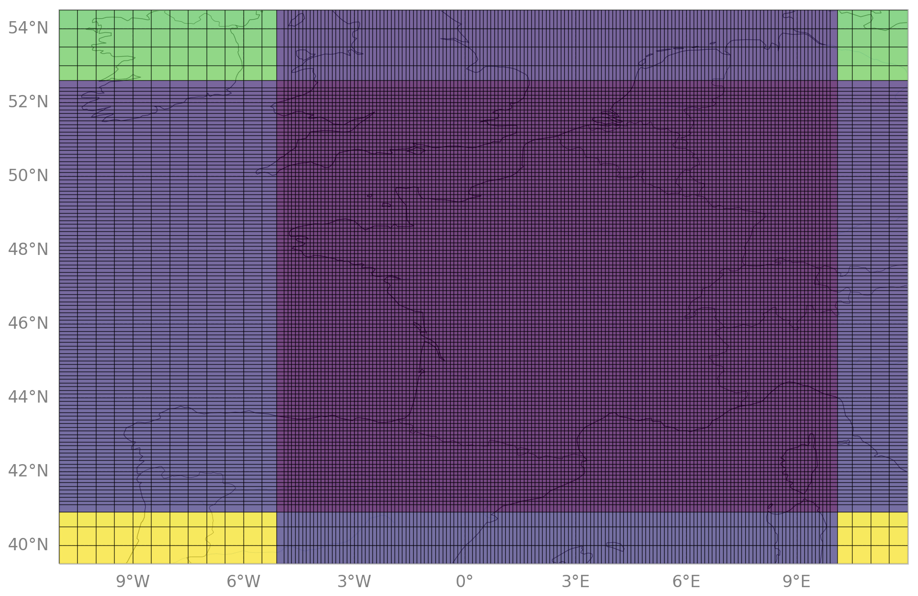
Figure 1Domain of our CHIMERE configuration: 10 km resolution regular sub-grid in purple, 50 km resolution in green and yellow, and 10 km × 50 km resolution in blue.
These emission maps have been aggregated to the grid of CHIMERE for the years 2019 to 2021 (Sect. 2.2 and Fig. 1).
2.2 Configuration of the CHIMERE CTM
We use the CHIMERE v2013 model to simulate fields of concentrations of gaseous chemical species in a domain that covers France and its vicinity (39.5–54.5° N, 11° W–12° E; see Fig. 1). The model horizontal grid is zoomed (Siour et al., 2013), with a 10 km resolution regular sub-grid in the center of the domain covering the whole of France and a 50 km resolution in the corners of the domain (Fig. 1). It corresponds to 166 (longitude) × 122 (latitude) horizontal grid cells. The model has 20 vertical layers from the surface to 200 hPa, with 8 layers within the first 2km.
The model is driven by the European Centre for Medium-Range Weather Forecasts (ECMWF) global meteorological fields (Owens and Hewson, 2018). Both CHIMERE (Menut et al., 2013) and its adjoint code operate the MELCHIOR-2 chemical scheme with more than 100 reactions (Lattuati, 1997; Derognat et al., 2003), including 24 for inorganic chemistry. Considering the short lifetime of NO2, we do not consider its import from outside the domain: its boundary conditions are set to zero. Nevertheless, the lateral and top boundaries for other species, such as ozone (O3), nitric acid (HNO3), peroxyacetyl nitrate (PAN) and formaldehyde (HCHO), participating in the NOx chemistry are considered. Initial and boundary conditions when relevant are specified using a nested run of CHIMERE (Siour et al., 2013) over a European domain (31.75–74.25° N, 15.25° W–35.75° E) with a spatial resolution of 0.5°, which itself uses boundary and initial conditions from climatological values from the LMDz-INCA global model (Szopa et al., 2009).
The aerosol module of CHIMERE is not considered in the simulations and inversions, as the adjoint of this module is not available (Fortems-Cheiney et al., 2021; Savas et al., 2023).
2.3 TROPOMI–PAL observations
TROPOMI, launched on board Sentinel-5 Precursor (S5P) in October 2017, is in a near-polar sun-synchronous orbit (altitude of ∼ 824 km) with an ascending node equatorial crossing at ∼ 13:40 Mean Local Solar Time. With an orbital cycle of 16 d and 14 orbits a day, the satellite passes over the same geographical area every cycle of 227 orbits. With a swath as wide as 108° – approximately 2600 km on ground – TROPOMI provides daily coverage for NO2. Observations over our domain span from around 09:30 to 14:30 local time with data from 2 to 3 orbits per day, with the major coverage around noon (11:30 to 13:30).
An evaluation of the TROPOMI v1.3 product with surface remote sensing observations indicated a systematic low bias of TROPOMI NO2 tropospheric vertical column densities (TVCDs) of typically −23 % to −37 % in clean to slightly polluted conditions and as high as −51 % over highly polluted areas (Verhoelst et al., 2021) compared to ground-based measurements. This negative bias has been mainly attributed to a negative cloud height bias in the Fast Retrieval Scheme for Clouds from Oxygen absorption band (FRESCO) implementation (van Geffen et al., 2022b), and efforts have been made to correct it in the TROPOMI–PAL product (Eskes et al., 2021).
Here, we use the TROPOMI–PAL reprocessed data (Eskes et al., 2021), available from 2019 to 11 November 2021. We use a recent reprocessing of the TROPOMI data, called RPRO version 2.4, to cover the end of the year 2021. This latest reprocessing uses a new higher-resolution directional Lambertian-equivalent reflectivity derived from TROPOMI observations (van Geffen et al., 2022a). Nevertheless, the last evaluation of the TROPOMI RPRO v2.4 product with surface remote sensing observations still indicates significant biases of TROPOMI, with NO2 TVCDs of typically +13 % over clean areas to −40 % over highly polluted areas (Lambert et al., 2023). These biases could partly be explained by the relatively coarse horizontal resolution of the prior global TM5-MP profiles (1° × 1°) used in the retrieval process (which can be neglected when applying the retrieval averaging kernels to the model) (Douros et al., 2023). However, these biases are also largely attributed to systematic errors in the retrieved cloud pressure, surface albedo used, etc. (Boersma et al., 2016; Douros et al., 2023).
We select the data with a quality assurance (QA) value of 0.75 for both products, following the criteria of van Geffen et al. (2022b). The latest version of the TROPOMI NO2 Algorithm Theoretical Basis Document (ATBD) is now for product version 2.6 (TROPOMI ATBD of the total and tropospheric NO2 data products, KNMI and S5P-KNMI-L2-0005-RP, issue 2.4.0; van Geffen et al., 2022a).
2.4 Comparison between simulated and observed NO2 TVCDs
To make relevant comparisons between simulations and satellite observations, the averaging kernels (AKs), which are associated with each observed TVCD and represent the vertical sensitivity of the satellite retrieval (Eskes and Boersma, 2003), are applied to the simulated concentration field. Due to the over-sampling resulting from the model's horizontal resolution being coarser than the TROPOMI data, we aggregate spatially and temporally the TROPOMI observations at the CHIMERE resolution into so-called super-observations. Within a given grid cell and time step, the super-observation is the observation (TVCD and AKs) which is the closest to the mean of the TROPOMI TVCDs. The error associated with each super-observation is also derived from the observation closest to the mean value and is subsequently included in the total so-called “observation error” (see Sect. 2.5). Our derivation of the error associated with each super-observation is thus conservative compared to other studies (Boersma et al., 2016), where the super-observation uncertainty is reduced compared to that of individual observations.
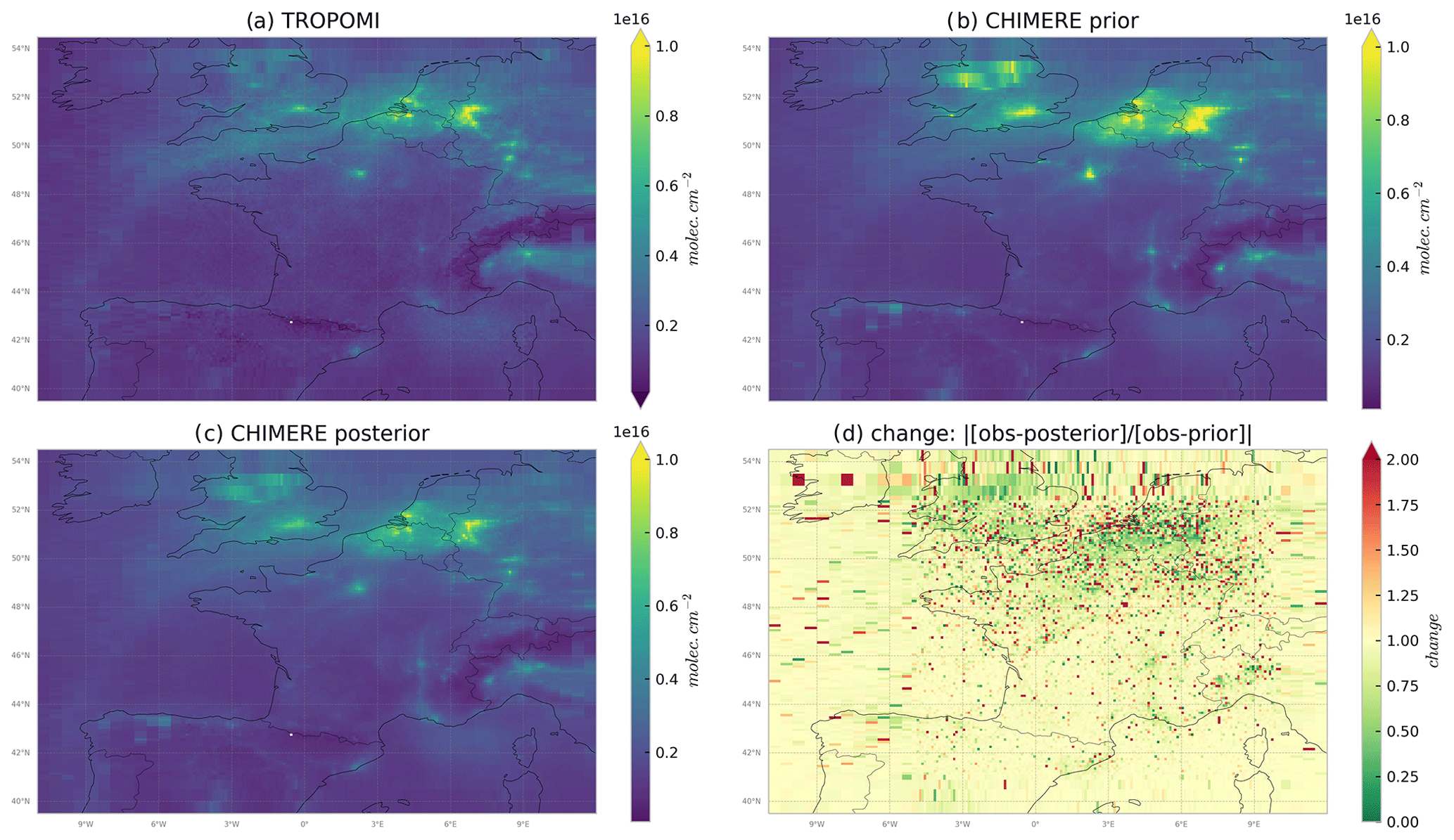
Figure 2Averages of NO2 TVCDs by (a) the TROPOMI–PAL data; (b) the CHIMERE simulation using prior emissions from CAMS-REG/INS and MEGAN, described in Sect. 2.1; and (c) the CHIMERE simulation using the posterior emissions from the inversion, for April 2020, in . (d) Ratio of the posterior and prior biases between NO2 TVCDs simulated with CHIMERE and the TROPOMI–PAL observations. All ratios lower than 1, in green, demonstrate that posterior emission estimates improve the simulation compared to the prior ones.
The reduction in uncertainty when combining several observations accounts for the fact that the retrieval errors include random noise (in particular, instrumental noise) without spatial correlation, i.e., errors which are independent from one observation to the other. However, as discussed above, the TROPOMI NO2 observations bear large systematic errors from the retrieval process, which can exhibit significant spatial correlations. This explains our conservative attribution of observation errors to the super-observations.
The corresponding column of NO2 in CHIMERE is vertically interpolated (at TROPOMI's super-observation location) on the vertical levels of the super-observation retrieval, and vertically integrated with the AKs of the super-observation, to yield the NO2 simulated TVCD to be compared to the super-observation TVCD, as illustrated in Fig. 2a and b for the month of April 2020.
2.5 Variational inversion of NOx emissions
The inversion of NOx emissions consists of correcting the prior estimate of the emissions (presented in Sect. 2.1) to improve the fit between NO2 TROPOMI–PAL satellite data and their simulated equivalents, using a Bayesian variational inversion framework similar to that of Fortems-Cheiney et al. (2021).
Series of 7 d inversion windows – independent from each other – are run and then combined to provide a corrected (“posterior”) estimate of NOx emissions over the whole period of analysis (2019–2021). For each inversion window, the posterior estimate of the emissions is found by iteratively minimizing the cost function J(x):
where x, ℋ, y, B and R are, respectively, the control vector, the observation operator, the satellite observations, the prior error covariance matrix and the observation error covariance matrix. The control vector x gathers variables for the correction of the surface NO and NO2 emissions, with xb corresponding to the prior estimate of the control vector.
Here the definition of x ensures that the inversion solves separately for the two main types of NO emissions, the anthropogenic and the biogenic emissions (without any further sectorization or decomposition into more detailed emission components), and for the anthropogenic NO2 emissions at the 1 d and model grid cell (i.e., 50 to 10 km) resolution temporally and horizontally and over three vertical levels for the anthropogenic emissions (accounting for the range of injection heights discriminating between the anthropogenic sources). With such a control vector, the prior NO / NO2 anthropogenic emission ratio speciation from the GENEMIS recommendations (see Sect. 2.1) is not conserved in the inversion, but the analysis focuses on the NOx emissions as the sum of the NO and NO2 emissions.
Furthermore, contrary to Fortems-Cheiney et al. (2021), we implicitly aim to characterize the prior uncertainty in both the anthropogenic and biogenic NOx emissions with log-normal distributions. This allows the inversion system to apply high variations in NOx emissions while ensuring positivity, unlike the classic corrections of the emission with scaling factors with a Gaussian distribution of prior uncertainty. However, the uncertainty in the control vector must follow a Gaussian distribution, as required by the use of Eq. (1). Therefore, here, the control vector x is defined as the logarithm of the scaling factors to be applied to the prior estimate of the emissions, and the posterior anthropogenic or biogenic emission estimate at a given grid cell of the model and for a given day fi is derived from the corresponding control parameter xi as .
Our control vector x is therefore characterized as follows:
-
It contains the logarithm of the scaling coefficients for NO anthropogenic emissions at a 1 d temporal resolution, for the 166 (longitude) × 122 (latitude) horizontal grid cells of the model, and over three vertical bands of injection heights for the emissions (from 0 to 25 m, from 25 to 1900 m and from 1900 to 12 000 m); this is done essentially to reduce the dimensionality of the problem along this axis, as most emissions are concentrated in the first two layers. The corrections applied are the same for all layers within a band.
-
It contains the logarithm of the scaling coefficients for NO2 anthropogenic emissions at the same temporal and spatial resolutions as for NO.
-
It contains the logarithm of the scaling coefficients for NO biogenic emissions at a 1 d temporal resolution, for the 166 (longitude) × 122 (latitude) model grid cells at the surface level.
NO and NO2 3D initial conditions (specified using a nested run of CHIMERE, as described in Sect. 2.2) are not controlled and are set once initially for all 7 d windows at 00:00 UTC on the first day of these windows. We therefore do not account for the potential update of the concentrations during a previous 7 d window due to the inversions. They have a low impact on the inversion, since the first satellite observations over the domain are around noon, while the NOx lifetime is short (on the order of a few hours; Hakkarainen et al., 2024).
The uncertainties in the observations y, together with those in the observation operator ℋ, and the uncertainties in the prior estimate of the control vector xb are assumed to have a Gaussian distribution. Therefore, they are fully characterized by error covariance matrices.
The prior uncertainty is defined at the resolution of the control vector. Thus, the terms of the prior error covariance matrix B reflect the uncertainties in the logarithm of the anthropogenic and biogenic emissions of NOx at 1 d and 50 to 10 km resolution. This matrix is set block diagonal (see Eq. 2), with one block corresponding to the anthropogenic emissions and the other one corresponding to the biogenic emissions, assuming that there is no correlation between the respective uncertainties in the prior estimates for these two types of emissions.
Another assumption is that, at the 1 d and 50 to 10 km resolution, there are no spatial or temporal correlations in the prior uncertainties in the anthropogenic emissions, due to the heterogeneity of these emissions. Therefore, the first block of B corresponding to the logarithms of the anthropogenic emissions is set diagonally. Each diagonal element is set at (0.3)2: the range associated to this σ value in the log-space corresponds to a factor ranging between 74 %–135 % in the emission space at the 1 d resolution and at the model's grid scale.
The second block of B corresponding to the biogenic fluxes accounts for space correlations in the uncertainties in these emissions, which are assumed to be more homogeneous in space and time than the anthropogenic emissions and to decrease exponentially with distance. They are set with a λ0 = 30 km decorrelation length. On the diagonal, uncertainties are set to a value of (0.6)2. The range associated to this value σ in the log-space corresponds to a factor ranging between 55 %–182 % in the emission space at the 1 d resolution and at the model's grid scale.
with ν in the form of .
ℋ is the observation operator, linking the control variables in the log-space to the simulated equivalents of the super-observations. It includes the exponential operator and scaling factor converting the maps of the logarithm of the coefficient for the emissions into emission maps at the spatial and temporal resolutions of CHIMERE, the atmospheric chemistry and transport model CHIMERE itself, and the extraction of the TVCDs from CHIMERE where and when we have TROPOMI super-observations.
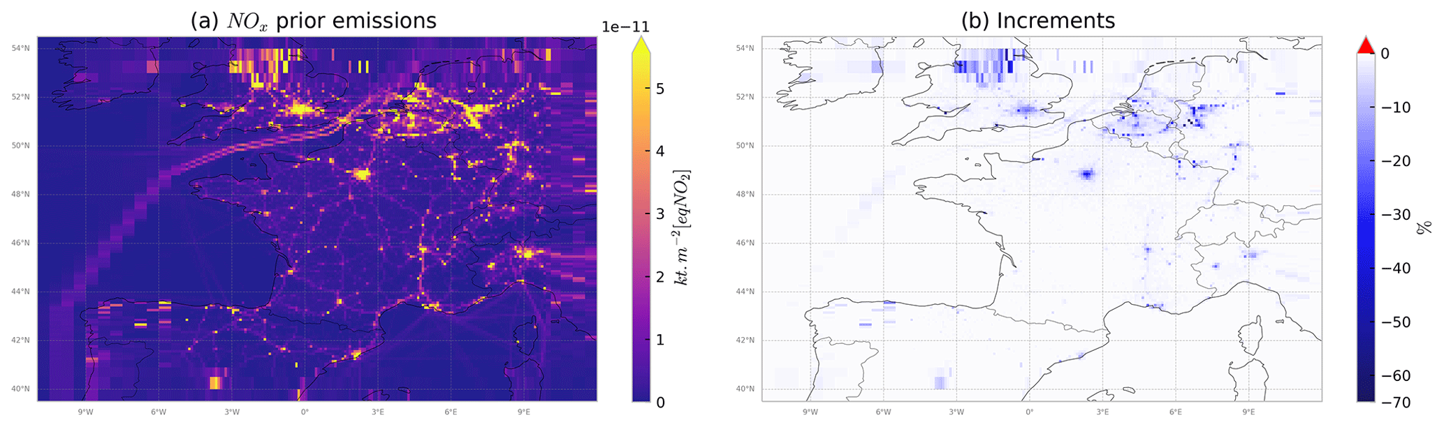
Figure 3(a) Total prior NOx fluxes (anthropogenic emissions from CAMS-REG/INS and biogenic emissions from MEGAN; see Sect. 2.1 for details) and (b) relative increments to the total prior emissions from the inversion in % for April 2020.
The uncertainties on the observations y and on the observation operator are characterized by the so-called observation error covariance matrix R, set up here as a diagonal matrix based on the assumption that these errors are not correlated in space or time when aggregated at the model 50 to 10 km and 1 h resolution. The variance in the observation errors corresponding to individual observations in the diagonal of R is the quadratic sum of the error we have assigned to the TROPOMI–PAL super-observations (see Sect. 2.4) and of an estimate of the errors from the observation operator. We assume that the observation operator error is dominated by the chemistry-transport modeling errors and by the errors associated with the discrepancies between the spatial representativity of the super-observations and of the model corresponding column: it is set at 30 % of the retrieval value. It was set at 20 % by Fortems-Cheiney et al. (2021) at a coarser resolution and is increased here to take into account the mismatch between the shape and location of the real and simulated atmospheric patterns at our finer resolution (see Sect. 2.4).
The minimum of the cost function J is searched for with the iterative M1QN3 limited-memory quasi-Newton minimization algorithm (Gilbert and Lemaréchal, 1989). At each iteration, the computation of the gradient of J relies on the adjoint of the observation operator and, in particular, on the adjoint of CHIMERE. In the results presented in Sect. 3, as a compromise between computational time and the level of convergence of the iterative minimization of J in the inversions, the minimization is regarded as satisfactory when the norm of the gradient of J is reduced by 80 %.
The calculation of the uncertainty in the posterior estimates of emissions is challenging when using a variational inverse system (Kadygrov et al., 2015; Rayner et al., 2019; Fortems-Cheiney et al., 2021), and it is not done here. It would require a large ensemble of time-consuming inversions (especially due to the handling of chemistry) to enable a proper sampling of the uncertainties and thus a proper derivation of the statistics of uncertainty.
3.1 Seasonal and inter-annual estimates of total French NOx emissions
3.1.1 Fit between TROPOMI–PAL super-observations and their simulated equivalents
Before analyzing the results in terms of emissions, we check the behavior of the inversion by comparing the performances of the prior and posterior simulations in reproducing the spatial and temporal variations of the observations. As an illustration, TROPOMI–PAL and the corresponding CHIMERE NO2 TVCDs are shown in Fig. 2a and b, respectively, for April 2020. The TROPOMI–PAL observations and their NO2 simulated equivalents present similar spatial patterns, with hotspots (TVCDs higher than 1 × 10¹⁶ ) over urban areas and low values over rural areas during the whole simulated period from 2019 to 2021 (illustrated in Fig. 2a and b for 1 month in 2020). However, the prior simulation overestimates the NO2 TVCDs over urban areas in France compared to the observations. For example, for April 2020, the mean bias between the prior simulation and TROPOMI is about 4.2 × 10¹⁴, 2.0 × 10¹⁴ and 3.8 × 10¹⁴ over Paris, Lyon and Marseille (Fig. A1), respectively. The inversion brings the simulated TVCDs closer to the TROPOMI–PAL data over urban areas (Fig. 2c): in this case, the mean bias and the mean root mean square over the three cities are reduced by about 30 % and 12 %, respectively.
As the CHIMERE prior simulation overestimates the NO2 TVCDs, the inversion brings the CHIMERE NO2 columns closer to the TROPOMI–PAL data by reducing NOx emissions, mainly over dense urban areas (Île-de-France, Lyon–Marseille axis, London area, Benelux, Frankfurt, Po Valley; see Fig. 3b). Over these areas, the relative corrections provided by the inversions to the total (anthropogenic and biogenic) emissions can reach −70 % (Fig. 3b).
3.1.2 Estimates of total French NOx emissions
This section focuses on the results from the NOx inversions in terms of comparisons between the total posterior NOx emissions and the prior ones. The focus on total emissions is explained by the fact that the distinction between the signal from the biogenic and anthropogenic emissions in the comparisons between the chemistry-transport model and the satellite NO2 observations is challenging in the inversion framework. Since both types of emissions are solved at the 1 d and model grid cell resolution, the inversion system relies on the respective amplitude and spatial correlations in the prior uncertainties in the biogenic and anthropogenic emissions (in B) to discriminate between the corrections to be applied to the prior estimates of the two types of emissions. However, our configuration of B yields similar structures of spatial correlations for the two types of emissions. Therefore, our confidence in the split between biogenic and anthropogenic emissions in the posterior emission estimates is low whenever the two types of emissions have comparable levels according to the prior emission estimates.
At the national scale, both the prior and the posterior emissions present a similar seasonal cycle in 2019–2021, with monthly emissions higher than 72 kteq NO2 during winter and equal to or lower than 66 kteq NO2 during summer (Fig. 4).
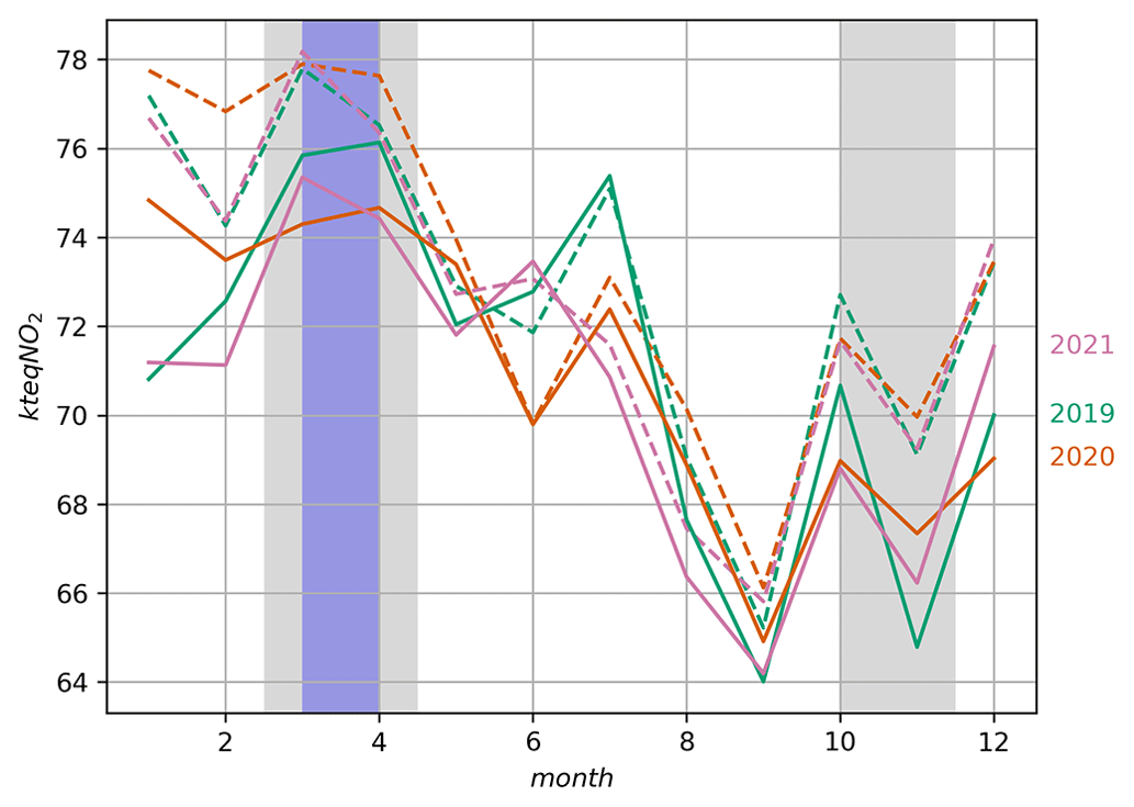
Figure 4Monthly total NOx emissions in France as estimated by CAMS-REG/INS and MEGAN (dotted lines) and by the inversions for the years 2019 (in green), 2020 (in orange) and 2021 (in pink), in kteq NO2 month−1. Gray shaded areas show the French lockdown periods for the year 2020, and the purple shaded area shows the French lockdown period for the year 2021.
Table 1Total prior and posterior NOx emission budgets in kteq NO2 and their relative differences in % for different periods in France. Columns “Posterior ” and “CITEPA ” show the relative difference between yearn and yearn−1 posterior fluxes and CITEPA in % .
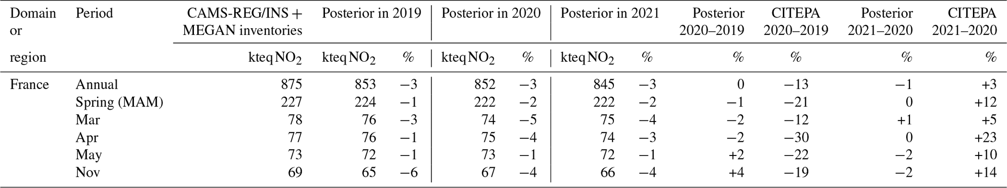
The mean French national budget for the years 2019 to 2021 from the total posterior emission estimates is about 850 kteq NO2, which is lower than the total prior emissions estimated from CAMS-REG/INS and MEGAN (average of 875 kteq NO2; Fig. 3, Table 1), with the largest reductions reaching about 8 % during fall and winter. This is expected, as public policies led to regular reductions in anthropogenic emissions between 2016 (our version of CAMS-REG/INS) and 2019–2021. The decrease in total NOx emissions is estimated at −13 % from 2016 to 2019 by the French Technical Reference Center for Air Pollution and Climate Change (CITEPA report; we use the estimates for “out-of-scope” natural emissions which are not reported to UNFCCC). According to CITEPA, the reduction is driven by large reductions in emissions from three major sectors between 2016 and 2019: the energy sector (−28 %), the industry sector (−22 %) and the transport sector (−15 %). However, the decrease found in this work is only about −3 % (Table 1). This can be explained by our configuration with neither spatial nor temporal correlation in our B matrix, leading to null or very small correction of the prior emissions from the inversions when the coverage of the country by TROPOMI super-observations is very sparse (Zheng et al., 2020). In this case, the posterior emissions remain close to the prior emission estimate and therefore at their 2016 levels (see Sect. 3.2.3).
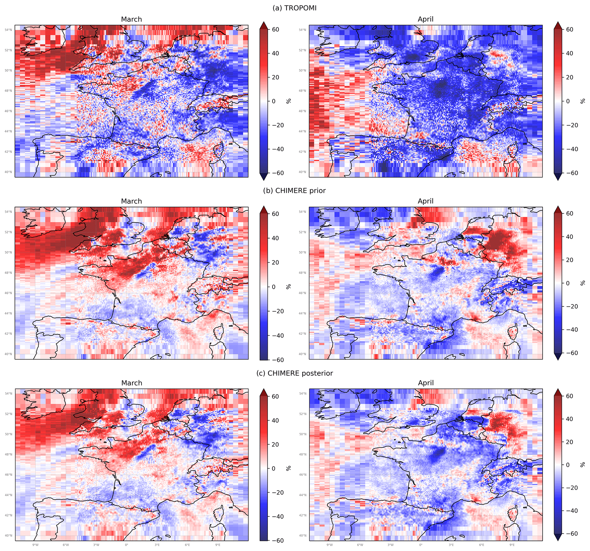
Figure 5Monthly gridded relative differences between monthly averages of (a) TROPOMI–PAL NO2 tropospheric columns, (b) CHIMERE prior tropospheric columns and (c) CHIMERE posterior tropospheric columns estimated by the inversions from March/April 2019 to March/April 2020, in % .
The 2019–2021 inter-annual variability is smaller with our inversions (Table 1) than in the estimates from CITEPA: the annual budget of the total French posterior NOx emissions varies by less than 1 % from year to year, while CITEPA estimates a decrease of about 13 % in 2020 compared to 2019 and an increase of about 3 % in 2021 compared to 2020 (Table 1). The similar total annual emissions in 2019 and 2020 nevertheless overlay different sub-annual variations. Higher emissions – partly associated with higher TROPOMI NO2 tropospheric columns (not shown) – are estimated in January, February, June and November 2020 compared to 2019 (Fig. 4). These increases counterbalance the decrease in NOx emissions in March/April 2020 (Figs. 4 and 5) which could be associated both with the COVID-19 crisis and with meteorological conditions with a warmer winter in 2020 than in 2019 (see Sect. 3.2.2).
When considering the split between biogenic and anthropogenic emissions from the inversions, despite its lack of reliability, the posterior biogenic emission estimates are close to the prior estimates derived from MEGAN (see Figs. C1 and C2): in particular, they do not appear to be stronger in 2020 than in 2019. Therefore, the low decrease (−3 %) in the posterior estimate of the national budget of the total NOx emissions in 2020 can hardly be explained by an increase in the biogenic emissions, which would compensate for the decrease in the anthropogenic emissions, even though the biogenic emissions due to agriculture were overlooked in our inversion setup (see Sect. 2.1).
3.2 Impact of the COVID-19 lockdown in spring 2020
The atmospheric lifetime of NO2 dictates that the high-spatial-resolution measurements from TROPOMI should readily capture rapid week-to-week changes in near-surface emissions (Levelt et al., 2022) and should therefore make it possible to assess the impact of the COVID-19 lockdown in spring 2020 on French NOx emissions. Following a usual diagnostic in the literature to assess the change in air pollutant concentrations due to COVID-19 policies, we characterize the impact of the first COVID-19 lockdown in France – occurring from 17 March to 10 May 2020 – in terms of changes from spring 2019 to spring 2020. Our analysis relies on the spatial distribution of the main areas of anthropogenic activities to identify the locations where the total NOx emissions should be dominated by anthropogenic emissions.
Table 2Changes in TROPOMI–PAL and CHIMERE NO2 tropospheric columns (in %) and changes in total posterior NOx emissions (in %), between March/April 2019 and March/April 2020 for the eight French urban areas displayed in Fig. A1.
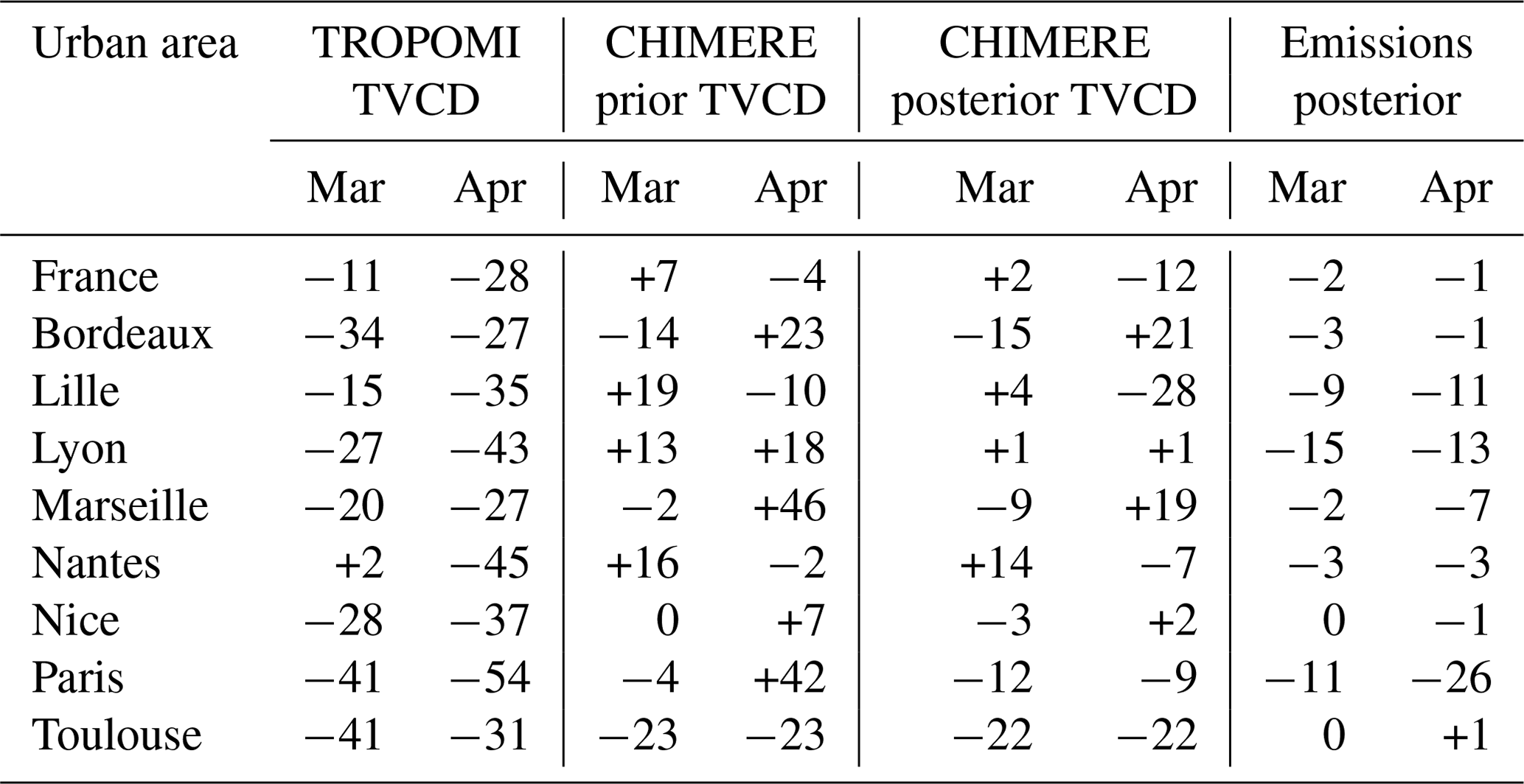
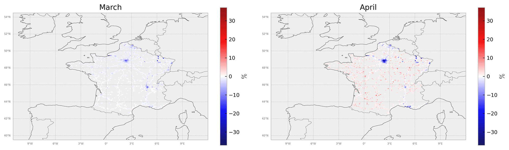
Figure 6Monthly gridded relative differences between the monthly total (anthropogenic + biogenic) posterior emissions estimated by the inversions from March/April 2019 to March/April 2020, for the months of March/April, using an urban and road land-use proxy (see Fig. C3), in % .
3.2.1 General impact on NO2 TROPOMI TVCDs
The TROPOMI NO2 TCVDs in March/April 2020 are first compared to 2019 at the national scale (Table 2). The TROPOMI NO2 TCVDs decrease from 2019 to 2020 by −11 and −28 %, respectively, in March/April over France. Similar decreases have been diagnosed in the measurements at surface stations over Europe with reductions in the average concentrations of NO2 of about −25 % for at least 75 % of the 1308 European Air Quality e-Reporting database (AirBase) stations compared with the average of the previous 7 years (2013–2019) for the period 18 March–18 May 2020 (Deroubaix et al., 2021).
The population distribution is heterogeneous in France, with large rural areas (i.e., 75.7 % of the country area, according to the French National Institute of Statistics and Economic Studies, 2020). We focus here on eight urban areas which correspond to hotspots of NOx concentrations and where, as a consequence, we expect a stronger signal due to changes in anthropogenic activities (Fig. A1): Paris, Lyon, Marseille, Lille, Bordeaux, Toulouse, Nice and Nantes.
The strength of the TROPOMI NO2 signal differs over these eight French cities. Indeed, the absolute changes in NO2 TVCD in March/April 2020 compared to March/April 2019 are higher for Paris, Lille, Lyon and Nantes (see Fig. C5) than for Bordeaux, Marseille, Nice and Toulouse (i.e., 1 × 10¹⁵ or less). The population density difference between those cities could partly explain such variability (Table A1).
TROPOMI NO2 tropospheric columns in March/April 2020 are 26 % to 38 % lower on average than in 2019 over the eight urban areas (Table 2). The relative changes from April 2019 to April 2020 range from −54 % for Paris to −27 % in Bordeaux (Table 2). This relative change over Paris is consistent with the decrease of −52 % described by Levelt et al. (2022) and with the decrease of about −56 % estimated by the tropospheric NO2 columns measured by two UV–visible Système d'Analyse par Observation Zénithale instruments (SAOZ; Pazmiño et al., 2021).
The temporal variability in the changes from spring 2019 to spring 2020 also differs from one urban area to another. With the exception of Bordeaux and Toulouse, the reductions in TVCDs are higher in April 2020 (Fig. 6, Table 2) than in March 2020 (Fig. 5, Table 2). This is consistent with the fact that the French population was confined only from mid-March (i.e., on 17 March versus the whole of April in 2020).
3.2.2 Various factors contributing to the differences in concentrations from spring 2019 to spring 2020 other than the lockdown
The relative changes in the TROPOMI TVCDs from spring 2019 to spring 2020 are partly due to COVID-19 lockdowns, but they are also driven by the changes in the meteorological and atmospheric chemistry-transport conditions (Menut et al., 2020; Diamond and Wood, 2020; Petetin et al., 2020; Barré et al., 2021; Gaubert et al., 2021; Deroubaix et al., 2021).
The differences from spring 2019 to spring 2020 in the simulated CHIMERE prior NO2 TVCDs (Fig. 5) are mainly due to changes in the meteorology and to a lesser extent to changes in the model boundary conditions and in the biogenic emissions (Sect. 2.2), as the prior anthropogenic emissions are the same in 2019 and in 2020 (Sect. 2.1).
CHIMERE prior NO2 TVCDs are 23 % higher in March 2020 than in March 2019 in the northern part of France, except for the plume of Paris. These changes thus have a sign which is opposite to the changes expected from the COVID-19 lockdowns. This is in agreement with the analysis of Gaubert et al. (2021), who showed that, when considering only the effect of meteorological variability, the level of NO2 concentrations would have been high during the 15 March–14 April 2020 period compared to the average NO2 concentrations in the same period over the 5 previous years (2015–2019) in the northwestern part of France (i.e., the Brittany, Pays de la Loire, Normandy and Hauts-de-France regions; Fig. 5).
CHIMERE prior NO2 TVCDs are 4 % lower in April 2020 than in April 2019 over almost the entire country (except above Paris and in the Rhône Valley). This is consistent with temperatures above seasonal values (by 3 °C over France, ranking as the third-warmest April on record), and with persistent anticyclonic conditions in April 2020 (MeteoFrance, 2022).
CHIMERE posterior NO2 TCVDs are about 12 % lower in April 2020 than in April 2019 over almost the entire country (Fig. 5, Table 2); a focus at the city scale shows a decrease of about 9 % over Paris between April 2019 and April 2020, whereas the prior NO2 TCVDs increase by about 42 % (Table 2).
Finally, the meteorological conditions also have an impact on the availability of the satellite observations. Due to the more favorable meteorological conditions with less cloud coverage leading to an unusual clear-sky period in April 2020 (Gaubert et al., 2021; Deroubaix et al., 2021), there is a higher number of TROPOMI observations in April 2020 than in March 2020 and than in 2019, particularly over the northeastern part of France (Fig. C4), which may allow a better correction of the CHIMERE NO2 TCVDs for this particular period (Sect. 3.2.3).
3.2.3 Impact on anthropogenic NOx emissions from spring 2019 to spring 2020
At the French national scale, the total NOx emission estimates from the inversions present their largest decrease during the first lockdown in March and April 2020 compared to in 2019 (Fig. 4). The emissions between May and September 2020 are similar to those in 2019 (Fig. 4), coinciding with the ease of restrictions. Nevertheless, the decrease in NOx emissions from March/April 2019 to March/April 2020 of about −2 % and −3 %, respectively, at the national scale is relatively flatter than the estimations found in the literature. For example, CITEPA estimates reductions of about −12 % and −30 % (Table 1), respectively, from March/April 2019 to March/April 2020 at the French national scale. Meteorology with a warmer winter can explain part of the changes in emissions between 2019 and 2020 for business sectors such as the residential combustion (Barré et al., 2021; Guevara et al., 2023).
We thus analyze the impact of the COVID-19 policies in terms of differences in retrieved anthropogenic emission estimates from the inversion from spring 2019 to spring 2020. For this, we focus on urban areas, assuming that the emissions in these pixels (see Fig. A1 for the chosen locations) are almost entirely due to anthropogenic activities.
In our inversions, the changes are negative in seven of the eight chosen urban areas (Fig. 6, Table 2), qualitatively consistent with the reduction in the intensity of vehicle traffic (Guevara et al., 2021, 2022). The changes are also negative for urban areas outside France in our domain (Table B2). The impact of the lockdown on anthropogenic NOx emissions is very different from one urban area to another. These differences between cities cannot be explained by different contributions of industry to NOx emissions in or around these urban areas, as INS data do not show major differences in terms of sectoral distribution between the main French cities.
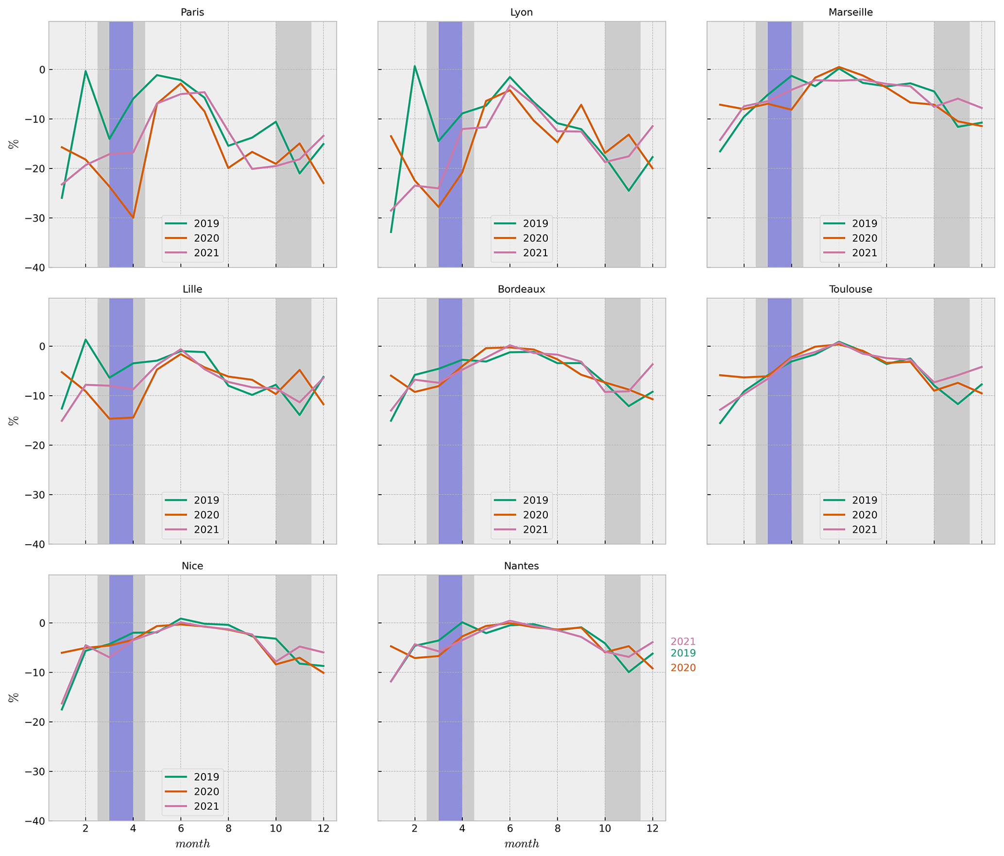
Figure 7The monthly budget relative differences in anthropogenic NOx emissions between posterior and prior for the eight French urban areas displayed in Fig. A1, from inversion results for the years 2019 (in green), 2020 (in orange) and 2021 (in pink), in %. Gray shaded areas show the French lockdown periods for the year 2020, and purple shaded areas show the French lockdown period for the year 2021.
The highest reductions are seen in Paris with about −26 % in April 2020 compared to April 2019, followed by Lyon (−13 %) and Lille (−11 %; Table 2). Several urban areas only present a very small drop in emissions in spring 2020 (Table 2, Fig. 7), e.g., the French urban areas Bordeaux, Nice and Nantes. The Toulouse urban area even shows a slight increase (+1 %) in April 2020 compared to April 2019 (Table 2, Fig. 7).
These small changes in emissions over Bordeaux, Nice and Toulouse do not seem consistent with the drops in traffic activity estimated by the Centre d'études et d'expertise sur les risques, l'environnement, la mobilité et l'aménagement (CEREMA; CEREMA, 2023). A dedicated study might be necessary to understand the inter-urban variability in detail and is not performed here, as up-to-date local inventories are not available for every city, particularly smaller ones.
The reductions in the anthropogenic NOx emissions from spring 2019 to spring 2020, while substantial, do not exhibit the same magnitude as the reductions in TROPOMI–PAL NO2 TVCDs. This is expected because of the non-linearities between anthropogenic NOx emissions and NO2 TVCDs but also due to the limitations and assumptions of the inversion itself.
3.2.4 Exploring limitations in our analysis
The discrepancy between the emission changes from 2019 to 2020 between the inversion results and independent estimates from inventories (i.e., CITEPA, CEREMA) can be partly connected to our conservative characterization of the uncertainties in the prior emission estimates, which ignores potential spatial and temporal correlations in the prior uncertainties in the anthropogenic emissions at the daily and 10 to 50 km resolution. Therefore, the direct information from the satellite observations is not extrapolated by the inversion in space and time via correlations in the B matrix; thus the departure of the inversion from the prior emission estimates is highly sensitive to the observation coverage and to its footprint in the emission field.
In this context, the corrections provided by the inversions to the prior emissions can be limited by the fact that the potential of TROPOMI to provide information is hampered by the cloud coverage. When considering the annual to monthly budgets of the emissions over all days (with and without observations), the amplitude of the corrections to the prior estimate of the emissions driven by the satellite observations is artificially decreased by the lack of corrections during days when there are no satellite observations.
Table 3Changes in CHIMERE total posterior NOx emissions for the standard (in %) and with a simplified observation error setup (in %), R matrix without model error; see details in Sect. 3.2.3 from March/April 2019 to March/April 2020 considering different TROPOMI coverage for the eight French urban areas displayed in Fig. A1.
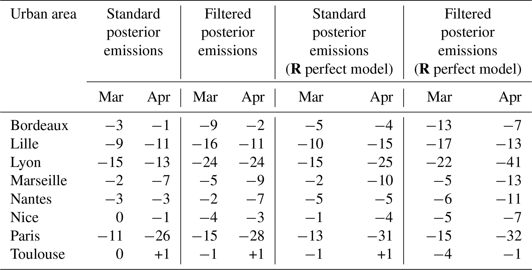
We quantify this effect by selecting days when we have at least one super-observation over the pixel of the eight urban areas of interest and extrapolating the retrieved emissions for this subset of days to the whole year, hereafter called “filtered emissions”. The reductions in the anthropogenic NOx filtered emissions from spring 2019 to spring 2020 are almost always higher than for the standard posterior emissions (e.g., −28 % and −24 % over Paris and over Lyon, respectively, for filtered emissions versus −26 % and −13 %; Table 3). These results with such a focus on days with the best coverage are in principle much closer to the changes in emissions estimated by CITEPA.
The corrections provided by the inversions to the prior emissions are also highly dependent on the errors associated with the TROPOMI–PAL observations and with the CTM errors in R. We illustrate this effect by performing an inversion without model errors in the covariance matrix R, giving more weight to the satellite data and regarding the model as perfect. The posterior NOx emissions retrieved with this error setup at the city scale show a higher reduction from spring 2019 to spring 2020 (Tables 3 and B3), e.g., −31 % and −25 % over Paris and over Lyon when using all the available observations and −33 % and −42 % for filtered emissions compared to −26 % and −13 % for the reference emissions.
Nevertheless, several urban areas still present a very small drop in emissions even when selecting days with observation and regarding the model as perfect to give more weight to the TROPOMI data. This is the case of the French urban areas Bordeaux, Nice and Toulouse with reductions from spring 2019 to spring 2020 lower than 10 % (Table 3).
This may be explained by the strength of the TROPOMI signal over these cities (see Sect. 3.2.1).
Filtered cases are only indicative, as this approach necessitates extrapolating from a notably small sample (days with observations; 16 and 19 d on average for the studied French cities in March and April 2020).
To gain emission representativity, we suggest exploring a fine-tuning of the correlation in B (with optionally additional information on NO2 concentrations like surface stations) to compensate for when TROPOMI data availability is lower. Despite our hypothesis made in Sect. 2.5 on anthropogenic fluxes, this might be necessary in addressing nation-wide NOx emission monitoring with a high local resolution.
We performed a 3-year variational inversion of NOx emissions from 2019 to 2021 in France at the high resolution of 10 km × 10 km. The TROPOMI–PAL observations were assimilated within the inversion system CIF driving the regional CTM CHIMERE with the MELCHIOR-2 chemical scheme.
The French budget for the years 2019, 2020 and 2021 is about 850 kteq NO2. As expected from the implementation of public policies leading to regular reductions in emissions, these national budgets from the inversions are lower than CAMS-REG/INS for 2016, used as the prior in our inversions. In particular, 2020 does not show a clear reduction in emissions compared to 2019: 2020 emissions are higher compared to 2019 in January, February, June and November. These increases dampen the decline in NOx emissions in March/April 2020 compared to March/April 2019.
We focus on the changes in NO2 TROPOMI–PAL TVCDs and in anthropogenic NOx emissions in March and April 2020 compared to 2019 that are due to the lockdowns during the COVID-19 pandemic and to meteorological conditions, including a milder winter (Barré et al., 2021; Guevara et al., 2023). Since inversions mainly detect changes in cities (hotspots), the main changes between March/April 2019 and March/April 2020 are observed at the city scale. However, the impacts of restrictions can vary significantly between different urban areas. Among the eight selected French urban areas, the relative changes between April 2020 and April 2019 in the TROPOMI–PAL observations range from −54 % for Paris to −27 % in Bordeaux. The highest reductions in anthropogenic NOx emissions, when we focus on days with observations, are seen in Paris with about −28 % in April 2020 compared to April 2019, followed by Lyon (−24 %) and Lille (−11 %).
Several urban areas, such as Bordeaux, Nice and Toulouse, only show a small decrease in emissions from spring 2019 to spring 2020, even when focusing on the results from the inversion over days with at least one super-observation and even when more weight is given to the TROPOMI data in the inversion process by assuming that the model is perfect. This may be due to weaker TROPOMI signals over these cities, with NO2 TVCD changes in March/April 2020 compared to March/April 2019 being smaller than those observed in Paris, Lyon and Lille.
The inversion results show significant decreases in the emissions from the largest cities in France from 2019 to 2020, but this decrease remains lower than that documented in most studies on this topic and by independent inventories (i.e., CITEPA and CEREMA). This can be partly connected to our conservative characterization of the prior emission uncertainties, since we ignore potential spatial and temporal correlations in the prior uncertainties in the anthropogenic emissions, so that the departure from the prior emission estimates in the inversion is highly sensitive to the observation coverage and emission footprints. The corrections provided by the inversions to the prior emissions can indeed be limited by the cloud coverage affecting the TROPOMI observations and by errors in the TROPOMI data and in the CTM. Notably, when TROPOMI observations are unavailable, the correction of prior emissions in the unconstrained pixels through inversions is null, resulting in posterior emissions remaining close to the prior ones. Hence, the aggregation of posterior emissions into monthly or yearly budgets leads to a dampening of the signal provided by TROPOMI. In order to better emphasize the direct information from the satellite observations, some of our analyses of the local urban emissions are focused on days with at least one observation in the targeted pixels, yielding a characterization of the COVID-19 effects which is more consistent with the changes in emissions estimated by CITEPA.
To explore the impact of the setup of error covariance matrices, we considered inversions without error models in the covariance matrix R, giving more weight to satellite data. In this case, the posterior NOx emissions at the city scale exhibit their highest reductions between spring 2019 and spring 2020 (e.g., −31 % and −25 % over Paris and over Lyon, respectively, considering all days within the month). Assimilating the observations without accounting for the model errors may lead to over-fitting and thus project these errors onto the emission estimates. However, the weight of R in our inversions may have to be re-assessed with regard to the relatively conservative option that we use here to assign observation error to the super-observations. A finer assessment would require a good knowledge of the share of retrieval errors between random noise without spatial correlations and more systematic errors with spatial correlations, as well as the typical length scales of such spatial correlations, which are currently challenging to derive (Miyazaki et al., 2012; Boersma et al., 2016; Lambert et al., 2023).
In the absence of alternative information, like new measurements from benchmark cities, reconciling our results with the existing literature would prompt a re-evaluation of the observation errors in our inversion and a potential reassessment of our model error definition. The information contained in TROPOMI TCVDs cannot be fully exploited in our inversion setup to get constraints on diffuse emissions, e.g., in French rural areas.
For improving diagnostics of monthly to annual emissions at national scale for emission hotspots, addressing challenges arising from satellite coverage gaps involves introducing horizontal, temporal and sectoral correlations in the covariance matrix B of the uncertainty in the gridded inventories with hourly variations that are used as prior estimates of the emissions by the inversions. Such a characterization would support the extrapolation in space and time of the information obtained locally for some days from the satellite observation. However, obtaining such correlations at high resolution poses a substantial challenge. The usual correlation models based on assumptions of isotropy, homogeneity in space and time, and decrease as a function of distance and time should poorly match the actual derivation and structures of gridded inventories convolved with typical temporal cycles at diurnal to seasonal scales, which is why a conservative configuration was used for the B matrix in this study (Super et al., 2020). The challenge is exacerbated when tackling a period such as 2019–2021, with lockdown measures in response to the COVID-19 crisis highly impacting the emissions and thus the structures of uncertainties in the emission inventories over large spatial scales but limited periods. Exploring corrections to parameters underlying inventories, such as the Fossil Fuel Data Assimilation System (FFDAS) for CO2, may actually support a cleaner extrapolation. Due to the current lack of knowledge about the statistics of the uncertainties in the gridded inventories used for the inversions, a stepwise approach is probably needed to tackle this general problem, gradually including some temporally varying spatial and temporal correlations in B and, in parallel, increasing efforts to diagnose these uncertainties. If achieved, these additions would assist the inversion system in implementing nationwide emission adjustments.
Furthermore, the incorporation of a hypothetical geostationary satellite (such as Sentinel-4) in conjunction with ground-based monitoring stations could enhance the temporal resolution and enable the capture of daily NOx cycles while also increasing the sensitivity of the satellite data near the surface.
The list of all 15 urban areas and their masks is displayed in the following figure. Each mask is made out of 10 km × 10 km pixels.
Table A1Cities studied in the paper and their areas in pixels with their population density according to EuroStat (statistics for 2019).
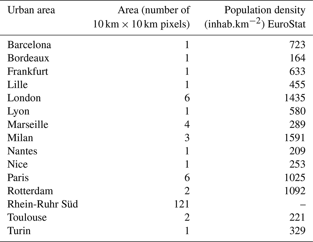
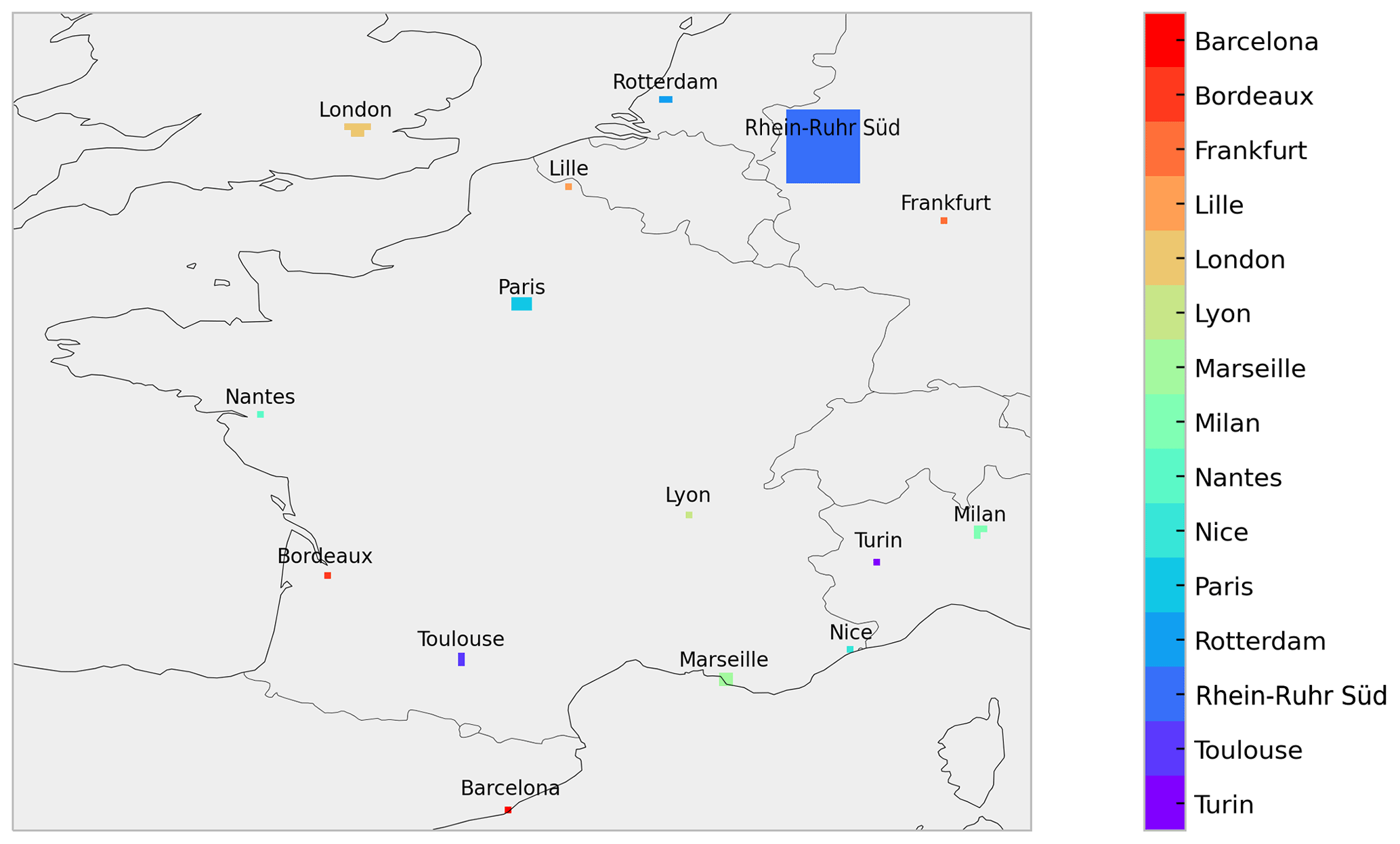
Figure A1Urban areas studied.
Table B1Total prior and posterior NOx emission budgets in kteq NO2 and their relative differences in % in Paris for different periods. Columns “Posterior ” show the relative difference between yearn and yearn−1 posterior fluxes in % .
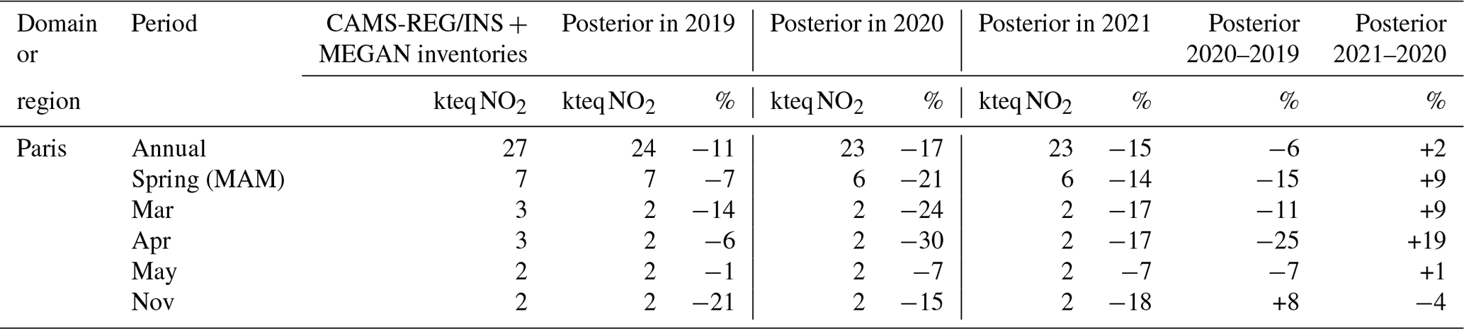
Table B2Changes in TROPOMI–PAL and CHIMERE NO2 tropospheric columns (in %) and changes in total posterior NOx emissions (in %) from March/April 2019 to March/April 2020 for the selection of urban areas displayed in Fig. A1.
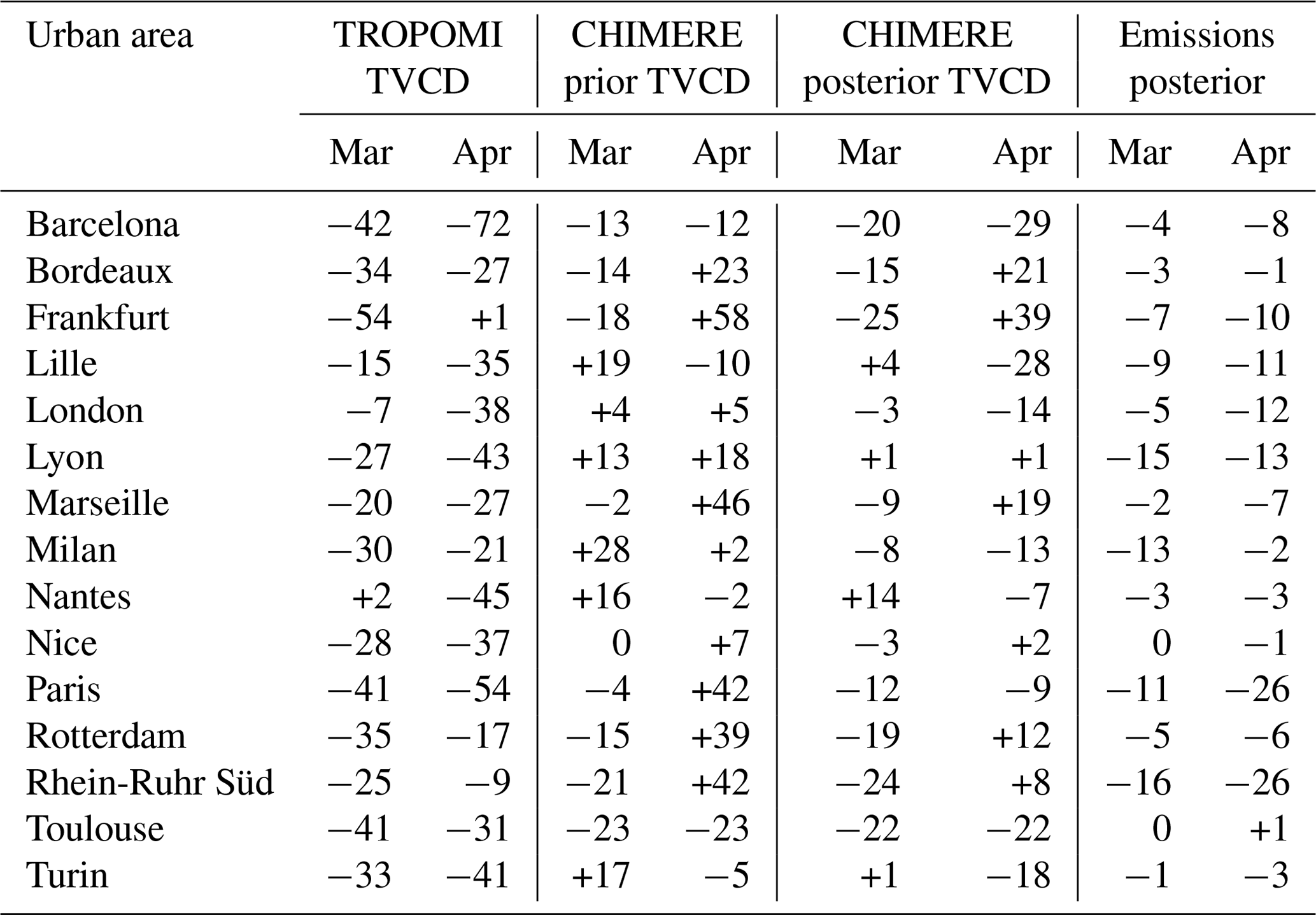
Table B3Changes in CHIMERE total posterior NOx emissions for the standard (in %) and with a simplified observation error setup (in %), R matrix without model error; see details in Sect. 3.2.3 from March/April 2019 to March/April 2020 considering different TROPOMI coverage for the selection of urban areas displayed in Fig. A1.
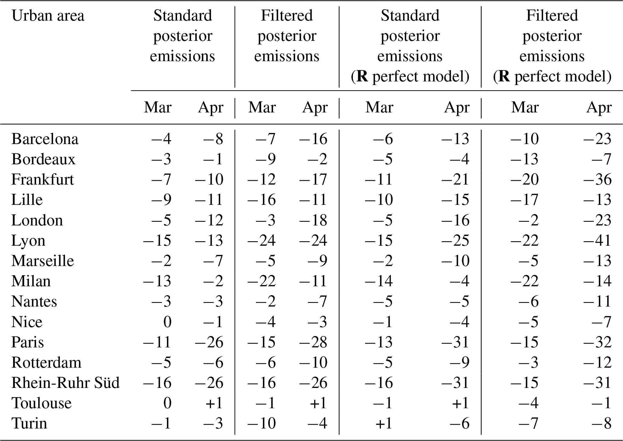
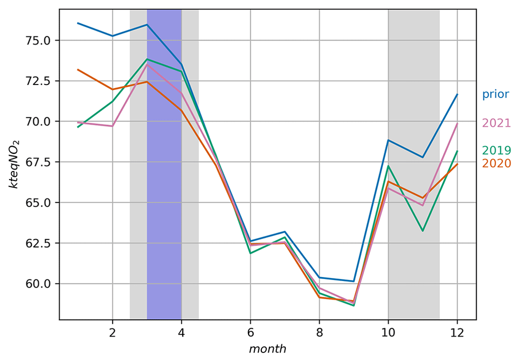
Figure C1Monthly anthropogenic NOx emissions in France as estimated by CAMS-REG/INS in 2016 (in blue) and by the inversions for the years 2019 (in green), 2020 (in orange) and 2021 (in pink), in kteq NO2 month−1. Gray shaded areas show the French lockdown periods for the year 2020, and the purple shaded area shows the French lockdown period for the year 2021.
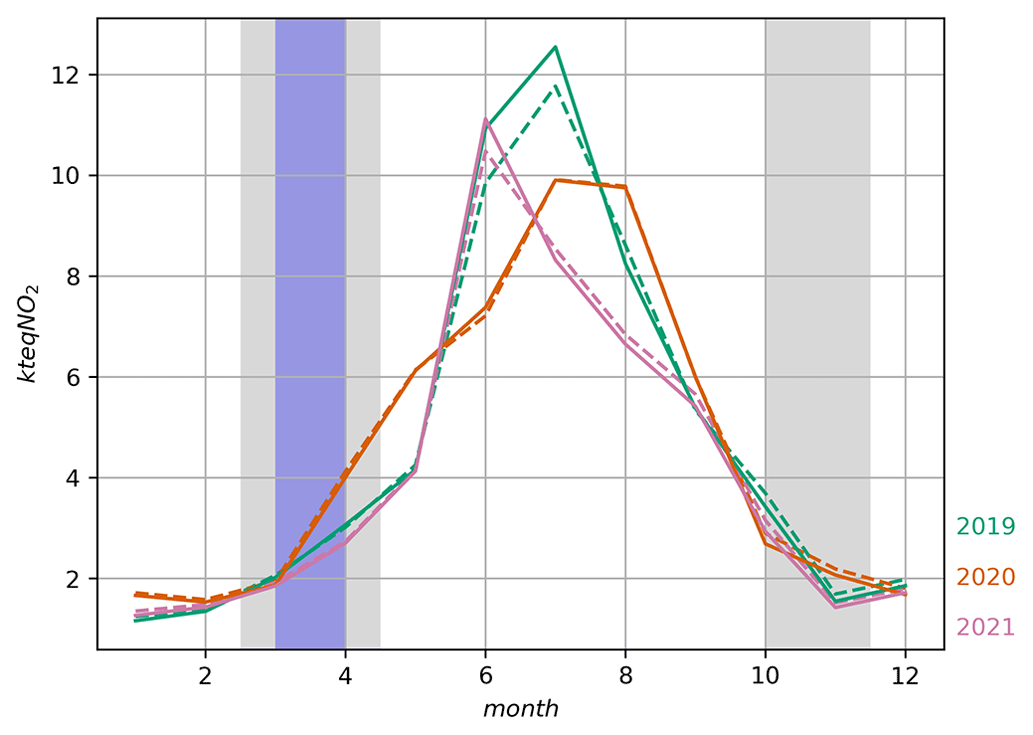
Figure C2Monthly biogenic NOx emissions in France as estimated by the MEGAN inventory (dotted lines) and by the inversions for the years 2019 (in green), 2020 (in orange) and 2021 (in pink), in kteq NO2 month−1. Gray shaded areas show the French lockdown periods for the year 2020, and the purple shaded area shows the French lockdown period for the year 2021.
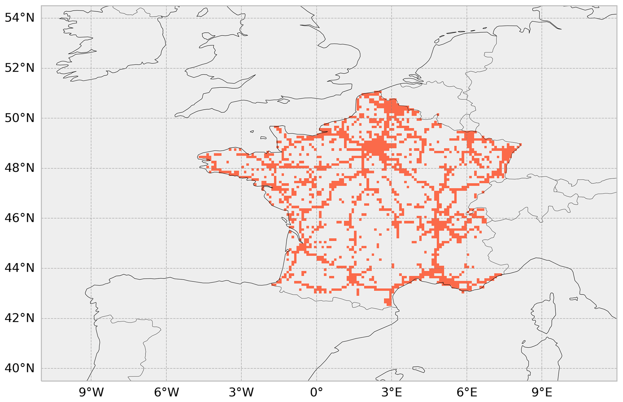
Figure C3Anthropogenic mask used over France using an urban and road land-use proxy.
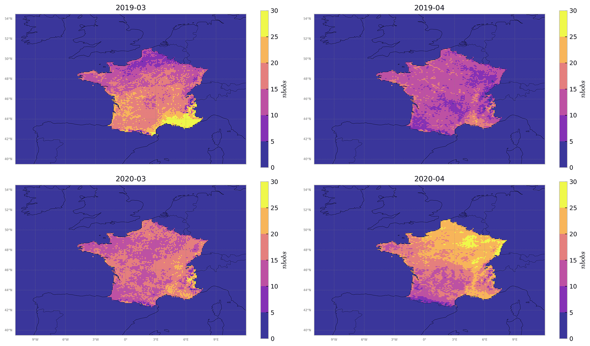
Figure C4Number of TROPOMI–PAL super-observations in the domain in March/April 2019 and March/April 2020.
The CHIMERE code (Menut et al., 2013; Mailler et al., 2017) is available at http://www.lmd.polytechnique.fr/chimere/ (CHIMERE, 2024). The CIF code (Berchet et al., 2021) is available at https://doi.org/10.5281/zenodo.6304912 (Berchet et al., 2022).
The reprocessed TROPOMI–PAL NO2 dataset (Eskes et al., 2021; S5P-PAL Data Portal, 2024) is available at https://dataspace.copernicus.eu/explore-data/data-collections/sentinel-data/sentinel-5p (Sentinal-5P, 2024). CAMS-REG (Kuenen et al., 2022) is available upon request from TNO (contact: Hugo Denier van der Gon, hugo.deniervandergon@tno.nl). The CITEPA monthly budgets for France (contact: Ariane Druart, ariane.druart@citepa.org) are available at https://www.citepa.org/fr/barometre/ (André et al., 2024). The INS inventory is available at http://emissions-air.developpement-durable.gouv.fr/ indexMap.html (INERIS, 2024).
RP, AFC, GB, IP, AB, EP, GD, AC, DS and GS conceptualized the study. GS produced the prior emissions map. HE produced the satellite data. RP and AFC carried out inversions and data analysis. All co-authors contributed to the design of the study and to writing the paper.
The contact author has declared that none of the authors has any competing interests.
Publisher's note: Copernicus Publications remains neutral with regard to jurisdictional claims made in the text, published maps, institutional affiliations, or any other geographical representation in this paper. While Copernicus Publications makes every effort to include appropriate place names, the final responsibility lies with the authors.
We thank the Netherlands Organisation for Applied Scientific Research (TNO) for the production and provision of the CAMS-REG data. We also thank the Institut national de l'environnement industriel et des risques (INERIS) for the production and provision of the INS data. We thank the anonymous referees for their insightful reviews and advices. This work was granted access to the HPC resources of TGCC under the allocations A0130102201 and A0140102201 made by GENCI. Finally, we thank Julien Bruna (LSCE) and his team for computer support.
This research has been supported by the Agence Nationale de la Recherche (ANR) ARGONAUT project (grant no. ANR-19-CE01-0007), the Agence de l'Environnement et de la Maîtrise de l'Energie (ADEME) PRIMEQUAL LOCKAIR project (grant no. 2162D0010), and the Centre National d'Etudes Spatiales (CNES) TOSCA ARGOS project (grant no. TOSCA ARGOS).
This paper was edited by Ilse Aben and reviewed by two anonymous referees.
Almaraz, M., Bai, E., Wang, C., Trousdell, J., Conley, S., Faloona, I., and Houlton, B. Z.: Agriculture is a major source of NOx pollution in California, Science Advances, 4, eaao3477, https://doi.org/10.1126/sciadv.aao3477, 2018. a
André, J.-M., Barrault, S., Bédrune, Q., Bonnot, M., Bongrand, G., Braish, T., Brier, É., Celeste, M., Cuniasse, B., Durand, A., Hercule, J., Juillard, M., Mazin, V., Mercier, A., Monti, V., Robert, C., Tresarrieu, A., Troncoso-Lamaison, F., Tuddenham, M., Vancayseele, C., Vieira Da Rocha, T., Grellier, L., Chang, J.-P., Allemand, N., and Druart, A.: CITEPA/Baromètre format Secten 2024, https://www.citepa.org/fr/barometre/ (last access: July 2024), 2024. a
Barré, J., Petetin, H., Colette, A., Guevara, M., Peuch, V.-H., Rouil, L., Engelen, R., Inness, A., Flemming, J., Pérez García-Pando, C., Bowdalo, D., Meleux, F., Geels, C., Christensen, J. H., Gauss, M., Benedictow, A., Tsyro, S., Friese, E., Struzewska, J., Kaminski, J. W., Douros, J., Timmermans, R., Robertson, L., Adani, M., Jorba, O., Joly, M., and Kouznetsov, R.: Estimating lockdown-induced European NO2 changes using satellite and surface observations and air quality models, Atmos. Chem. Phys., 21, 7373–7394, https://doi.org/10.5194/acp-21-7373-2021, 2021. a, b, c, d
Bauwens, M., Compernolle, S., Stavrakou, T., Müller, J.-F., Van Gent, J., Eskes, H., Levelt, P. F., Van Der A, R., Veefkind, J., Vlietinck, J., Yu, H., and Zehner, C.: Impact of coronavirus outbreak on NO2 pollution assessed using TROPOMI and OMI observations, Geophys. Res. Lett., 47, e2020GL087978, https://doi.org/10.1029/2020GL087978, 2020. a
Berchet, A., Sollum, E., Thompson, R. L., Pison, I., Thanwerdas, J., Broquet, G., Chevallier, F., Aalto, T., Berchet, A., Bergamaschi, P., Brunner, D., Engelen, R., Fortems-Cheiney, A., Gerbig, C., Groot Zwaaftink, C. D., Haussaire, J.-M., Henne, S., Houweling, S., Karstens, U., Kutsch, W. L., Luijkx, I. T., Monteil, G., Palmer, P. I., van Peet, J. C. A., Peters, W., Peylin, P., Potier, E., Rödenbeck, C., Saunois, M., Scholze, M., Tsuruta, A., and Zhao, Y.: The Community Inversion Framework v1.0: a unified system for atmospheric inversion studies, Geosci. Model Dev., 14, 5331–5354, https://doi.org/10.5194/gmd-14-5331-2021, 2021. a, b
Berchet, A., Sollum, E., Pison, I., Thompson, R. L., Thanwerdas, J., Fortems-Cheiney, A., van Peet, J. C. A., Potier, E., Chevallier, F., Broquet, G., and Berchet, A.: The Community Inversion Framework: codes and documentation (v1.1), Zenodo [code], https://doi.org/10.5281/zenodo.6304912, 2022. a
Bieser, J., Aulinger, A., Matthias, V., Quante, M., and Van Der Gon, H. D.: Vertical emission profiles for Europe based on plume rise calculations, Environ. Pollut., 159, 2935–2946, 2011. a
Boersma, K. F., Vinken, G. C. M., and Eskes, H. J.: Representativeness errors in comparing chemistry transport and chemistry climate models with satellite UV–Vis tropospheric column retrievals, Geosci. Model Dev., 9, 875–898, https://doi.org/10.5194/gmd-9-875-2016, 2016. a, b, c
Bovensmann, H., Burrows, J. P., Buchwitz, M., Frerick, J., Noël, S., Rozanov, V. V., Chance, K. V., and Goede, A. P. H.: SCIAMACHY: Mission Objectives and Measurement Modes, J. Atmos. Sci., 56, 127–150, https://doi.org/10.1175/1520-0469(1999)056<0127:SMOAMM>2.0.CO;2, 1999. a
Brand, C.: Beyond `Dieselgate': Implications of unaccounted and future air pollutant emissions and energy use for cars in the United Kingdom, Energy Policy, 97, 1–12, https://doi.org/10.1016/j.enpol.2016.06.036, 2016. a
Burrows, J., Hölzle, E., Goede, A., Visser, H., and Fricke, W.: SCIAMACHY–scanning imaging absorption spectrometer for atmospheric chartography, Acta Astronaut., 35, 445–451, https://doi.org/10.1016/0094-5765(94)00278-t, 1995. a
Burrows, J. P., Weber, M., Buchwitz, M., Rozanov, V., Ladstätter-Weißenmayer, A., Richter, A., DeBeek, R., Hoogen, R., Bramstedt, K., Eichmann, K.-U., Eisinger, M., and Perner, D.: The Global Ozone Monitoring Experiment (GOME): Mission Concept and First Scientific Results, J. Atmos. Sci., 56, 151–175, https://doi.org/10.1175/1520-0469(1999)056<0151:TGOMEG>2.0.CO;2, 1999. a
Cao, X.-Q., Liu, B.-N., Liu, M.-Z., Peng, K.-C., and Tian, W.-L.: Variational principles for two kinds of non-linear geophysical KdV equation with fractal derivatives, Therm. Sci., 26, 2505–2515, 2022. a
CEREMA: Indicateurs de trafic routier en France, Tech. rep., CEREMA, https://dataviz.cerema.fr/trafic-routier/ (last access: July 2024), 2023. a
CHIMERE: CHIMERE – A multi-scale chemistry-transport model for atmospheric composition analysis and forecast, current version: CHIMERE v2023r2, http://www.lmd.polytechnique.fr/chimere/ (last access: July 2024), 2024. a
Costa, S., Ferreira, J., Silveira, C., Costa, C., Lopes, D., Relvas, H., Borrego, C., Roebeling, P., Miranda, A., and Teixeira, J.: Integrating Health on Air Quality Assessment–Review Report on Health Risks of Two Major European Outdoor Air Pollutants: PM and NO2, J. Toxicol. Env. Health, 17, 307–340, https://doi.org/10.1080/10937404.2014.946164, 2014. a
Derognat, C., Beekmann, M., Baeumle, M., Martin, D., and Schmidt, H.: Effect of biogenic volatile organic compound emissions on tropospheric chemistry during the Atmospheric Pollution Over the Paris Area (ESQUIF) campaign in the Ile-de-France region, J. Geophys. Res.-Atmos., 108, 8560, https://doi.org/10.1029/2001JD001421, 2003. a
Deroubaix, A., Brasseur, G., Gaubert, B., Labuhn, I., Menut, L., Siour, G., and Tuccella, P.: Response of surface ozone concentration to emission reduction and meteorology during the COVID-19 lockdown in Europe, Meteorol. Appl., 28, e1990, https://doi.org/10.1002/met.1990, 2021. a, b, c, d
Diamond, M. S. and Wood, R.: Limited regional aerosol and cloud microphysical changes despite unprecedented decline in nitrogen oxide pollution during the February 2020 COVID-19 shutdown in China, Geophys. Res. Lett., 47, e2020GL088913, https://doi.org/10.1029/2020GL088913, 2020. a, b
Ding, J., Miyazaki, K., van der A, R. J., Mijling, B., Kurokawa, J.-I., Cho, S., Janssens-Maenhout, G., Zhang, Q., Liu, F., and Levelt, P. F.: Intercomparison of NOx emission inventories over East Asia, Atmos. Chem. Phys., 17, 10125–10141, https://doi.org/10.5194/acp-17-10125-2017, 2017. a
Douros, J., Eskes, H., van Geffen, J., Boersma, K. F., Compernolle, S., Pinardi, G., Blechschmidt, A.-M., Peuch, V.-H., Colette, A., and Veefkind, P.: Comparing Sentinel-5P TROPOMI NO2 column observations with the CAMS regional air quality ensemble, Geosci. Model Dev., 16, 509–534, https://doi.org/10.5194/gmd-16-509-2023, 2023. a, b
Ebel, A., Friedrich, R., and Rodhe, H.: GENEMIS: Assessment, improvement, and temporal and spatial disaggregation of European emission data, in: Tropospheric Modelling and Emission Estimation: Chemical Transport and Emission Modelling on Regional, Global and Urban Scales, Vol. 7, Springer, Berlin, Heidelberg, 181–214, https://doi.org/10.1007/978-3-662-03470-5_6, 1997. a
EEA: Air quality in Europe – 2020 report, Tech. rep., European Union, https://doi.org/10.2800/786656, 2020. a
EEA: Europe's air quality status 2023, EEA report, EEA, https://www.eea.europa.eu/publications/europes-air-quality-status-2023 (last access: July 2024), 2023. a
Elbern, H., Schmidt, H., Talagrand, O., and Ebel, A.: 4D-variational data assimilation with an adjoint air quality model for emission analysis, Environ. Modell. Softw., 15, 539–548, 2000. a
Elguindi, N., Granier, C., Stavrakou, T., Darras, S., Bauwens, M., Cao, H., Chen, C., Denier van der Gon, H. A. C., Dubovik, O., Fu, T. M., Henze, D. K., Jiang, Z., Keita, S., Kuenen, J. J. P., Kurokawa, J., Liousse, C., Miyazaki, K., Müller, J.-F., Qu, Z., Solmon, F., and Zheng, B.: Intercomparison of Magnitudes and Trends in Anthropogenic Surface Emissions From Bottom-Up Inventories, Top-Down Estimates, and Emission Scenarios, Earths Future, 8, e2020EF001520, https://doi.org/10.1029/2020ef001520, 2020. a
Eskes, H., van Geffen, J., Sneep, M., Veefkind, P., Niemeijer, S., and Zehner, C.: S5P Nitrogen Dioxide v02.03.01 intermediate reprocessing on the S5P-PAL system: Readme file, https://data-portal.s5p-pal.com/product-docs/no2/PAL_reprocessing_NO2_v02.03.01_20211215.pdf (last access: July 2024), 2021. a, b, c
Eskes, H. J. and Boersma, K. F.: Averaging kernels for DOAS total-column satellite retrievals, Atmos. Chem. Phys., 3, 1285–1291, https://doi.org/10.5194/acp-3-1285-2003, 2003. a
Fortems-Cheiney, A., Pison, I., Broquet, G., Dufour, G., Berchet, A., Potier, E., Coman, A., Siour, G., and Costantino, L.: Variational regional inverse modeling of reactive species emissions with PYVAR-CHIMERE-v2019, Geosci. Model Dev., 14, 2939–2957, https://doi.org/10.5194/gmd-14-2939-2021, 2021. a, b, c, d, e, f
Gaubert, B., Bouarar, I., Doumbia, T., Liu, Y., Stavrakou, T., Deroubaix, A., Darras, S., Elguindi, N., Granier, C., Lacey, F., Müller, J.-F., Shi, X., Tilmes, S., Wang, T., and Brasseur, G. P.: Global changes in secondary atmospheric pollutants during the 2020 COVID-19 pandemic, J. Geophys. Res.-Atmos., 126, e2020JD034213, https://doi.org/10.1029/2020JD034213, 2021. a, b, c, d
Gilbert, J. and Lemaréchal, C.: Some numerical experiments with variable storage quasi Newton algorithms, Math. Program., 45, 407–435, https://doi.org/10.1007/bf01589113, 1989. a
Guenther, A., Karl, T., Harley, P., Wiedinmyer, C., Palmer, P. I., and Geron, C.: Estimates of global terrestrial isoprene emissions using MEGAN (Model of Emissions of Gases and Aerosols from Nature), Atmos. Chem. Phys., 6, 3181–3210, https://doi.org/10.5194/acp-6-3181-2006, 2006. a
Guevara, M., Jorba, O., Soret, A., Petetin, H., Bowdalo, D., Serradell, K., Tena, C., Denier van der Gon, H., Kuenen, J., Peuch, V.-H., and Pérez García-Pando, C.: Time-resolved emission reductions for atmospheric chemistry modelling in Europe during the COVID-19 lockdowns, Atmos. Chem. Phys., 21, 773–797, https://doi.org/10.5194/acp-21-773-2021, 2021. a, b
Guevara, M., Petetin, H., Jorba, O., Denier van der Gon, H., Kuenen, J., Super, I., Jalkanen, J.-P., Majamäki, E., Johansson, L., Peuch, V.-H., and Pérez García-Pando, C.: European primary emissions of criteria pollutants and greenhouse gases in 2020 modulated by the COVID-19 pandemic disruptions, Earth Syst. Sci. Data, 14, 2521–2552, https://doi.org/10.5194/essd-14-2521-2022, 2022. a, b
Guevara, M., Petetin, H., Jorba, O., Denier van der Gon, H., Kuenen, J., Super, I., Granier, C., Doumbia, T., Ciais, P., Liu, Z., Lamboll, R. D., Schindlbacher, S., Matthews, B., and Pérez García-Pando, C.: Towards near-real-time air pollutant and greenhouse gas emissions: lessons learned from multiple estimates during the COVID-19 pandemic, Atmos. Chem. Phys., 23, 8081–8101, https://doi.org/10.5194/acp-23-8081-2023, 2023. a, b, c, d
Hakkarainen, H., Järvinen, A., Lepistö, T., Kuittinen, N., Markkula, L., Ihantola, T., Yang, M., Martikainen, M.-V., Mikkonen, S., Timonen, H., Aurela, M., Barreira, L., Ihalainen, M., Saarikoski, S., Rönkkö, T., Aakko-Saksa, P., and Jalava, P.: Effects of fuel composition and vehicle operating temperature on in vitro toxicity of exhaust emissions, Environmental Science: Atmospheres, 4, 455–467, https://doi.org/10.1039/D3EA00136A, 2024. a
Henze, D. K., Seinfeld, J. H., and Shindell, D. T.: Inverse modeling and mapping US air quality influences of inorganic PM2.5 precursor emissions using the adjoint of GEOS-Chem, Atmos. Chem. Phys., 9, 5877–5903, https://doi.org/10.5194/acp-9-5877-2009, 2009. a
INERIS: Inventaire National Spatialisé, http://emissions-air.developpement-durable.gouv.fr/indexMap.html (last access: July 2024), 2024. a
Kadygrov, N., Broquet, G., Chevallier, F., Rivier, L., Gerbig, C., and Ciais, P.: On the potential of the ICOS atmospheric CO2 measurement network for estimating the biogenic CO2 budget of Europe, Atmos. Chem. Phys., 15, 12765–12787, https://doi.org/10.5194/acp-15-12765-2015, 2015. a
Kuenen, J. and Dore, C.: EMEP/EEA air pollutant emission inventory guidebook 2019: Uncertainties, Tech. rep., EEA, https://www.eea.europa.eu/publications/emep-eea-guidebook-2019/part-a-general-guidance-chapters/5-uncertainties (last access: July 2024), 2019. a
Kuenen, J., Dellaert, S., Visschedijk, A., Jalkanen, J.-P., Super, I., and Denier van der Gon, H.: CAMS-REG-v4: a state-of-the-art high-resolution European emission inventory for air quality modelling, Earth Syst. Sci. Data, 14, 491–515, https://doi.org/10.5194/essd-14-491-2022, 2022. a, b, c, d, e
Lambert, J.-C., Keppens, A., Compernolle, S., Eichmann, K.-U., de Graaf, M., Hubert, D., Langerock, B., Ludewig, A., Sha, M., Verhoelst, T., Wagner, T., Ahn, C., Argyrouli, A., Balis, D., Chan, K., Coldewey-Egbers, M., Smedt, I. D., Eskes, H., Fjæraa, A., Garane, K., Gleason, J., Goutail, F., Granville, J., Hedelt, P., Ahn, C., Heue, K.-P., Jaross, G., Kleipool, Q., Koukouli, M., Lutz, R., Velarte, M. M., Michailidis, K., Nanda, S., Niemeijer, S., Pazmiño, A., Pinardi, G., Richter, A., Rozemeijer, N., Sneep, M., Zweers, D. S., Theys, N., Tilstra, G., Torres, O., Valks, P., van Geffen, J., Vigouroux, C., Wang, P., and Weber., M.: Quarterly Validation Report of the Copernicus Sentinel-5 Precursor Operational Data Products #21: April 2018–November 2023, Tech. rep., CAMS Cluster Service, https://mpc-vdaf.tropomi.eu/ProjectDir/reports//pdf/S5P-MPC-IASB-ROCVR-21.01.00.pdf (last access: July 2024), 2023. a, b
Lamsal, L. N., Martin, R. V., Padmanabhan, A., van Donkelaar, A., Zhang, Q., Sioris, C. E., Chance, K., Kurosu, T. P., and Newchurch, M. J.: Application of satellite observations for timely updates to global anthropogenic NOx emission inventories, Geophys. Res. Lett., 38, L05810, https://doi.org/10.1029/2010gl046476, 2011. a, b
Lattuati, M.: Impact des emissions Europeennes sur le bilan de l'ozone tropospherique a l'interface de l'Europe et de l'Atlantique Nord: apport de la modelisation Lagrangienne et des mesures en altitude, PhD thesis, Paris 6, https://www.sudoc.abes.fr/cbs/DB=2.1/SRCH?IKT=12&TRM=049559052 (last access: July 2024), 1997. a
Lee, S.-S., Chu, J.-E., Timmermann, A., Chung, E.-S., and Lee, J.-Y.: East Asian climate response to COVID-19 lockdown measures in China, Sci. Rep.-UK, 11, 16852, https://doi.org/10.1038/s41598-021-96007-1, 2021. a
Levelt, P. F., Joiner, J., Tamminen, J., Veefkind, J. P., Bhartia, P. K., Stein Zweers, D. C., Duncan, B. N., Streets, D. G., Eskes, H., van der A, R., McLinden, C., Fioletov, V., Carn, S., de Laat, J., DeLand, M., Marchenko, S., McPeters, R., Ziemke, J., Fu, D., Liu, X., Pickering, K., Apituley, A., González Abad, G., Arola, A., Boersma, F., Chan Miller, C., Chance, K., de Graaf, M., Hakkarainen, J., Hassinen, S., Ialongo, I., Kleipool, Q., Krotkov, N., Li, C., Lamsal, L., Newman, P., Nowlan, C., Suleiman, R., Tilstra, L. G., Torres, O., Wang, H., and Wargan, K.: The Ozone Monitoring Instrument: overview of 14 years in space, Atmos. Chem. Phys., 18, 5699–5745, https://doi.org/10.5194/acp-18-5699-2018, 2018. a
Levelt, P. F., Stein Zweers, D. C., Aben, I., Bauwens, M., Borsdorff, T., De Smedt, I., Eskes, H. J., Lerot, C., Loyola, D. G., Romahn, F., Stavrakou, T., Theys, N., Van Roozendael, M., Veefkind, J. P., and Verhoelst, T.: Air quality impacts of COVID-19 lockdown measures detected from space using high spatial resolution observations of multiple trace gases from Sentinel-5P/TROPOMI, Atmos. Chem. Phys., 22, 10319–10351, https://doi.org/10.5194/acp-22-10319-2022, 2022. a, b, c
Lin, J.-T.: Satellite constraint for emissions of nitrogen oxides from anthropogenic, lightning and soil sources over East China on a high-resolution grid, Atmos. Chem. Phys., 12, 2881–2898, https://doi.org/10.5194/acp-12-2881-2012, 2012. a
Mailler, S., Menut, L., Khvorostyanov, D., Valari, M., Couvidat, F., Siour, G., Turquety, S., Briant, R., Tuccella, P., Bessagnet, B., Colette, A., Létinois, L., Markakis, K., and Meleux, F.: CHIMERE-2017: from urban to hemispheric chemistry-transport modeling, Geosci. Model Dev., 10, 2397–2423, https://doi.org/10.5194/gmd-10-2397-2017, 2017. a, b
Menut, L., Goussebaile, A., Bessagnet, B., Khvorostiyanov, D., and Ung, A.: Impact of realistic hourly emissions profiles on air pollutants concentrations modelled with CHIMERE, Atmos. Environ., 49, 233–244, 2012. a
Menut, L., Bessagnet, B., Khvorostyanov, D., Beekmann, M., Blond, N., Colette, A., Coll, I., Curci, G., Foret, G., Hodzic, A., Mailler, S., Meleux, F., Monge, J.-L., Pison, I., Siour, G., Turquety, S., Valari, M., Vautard, R., and Vivanco, M. G.: CHIMERE 2013: a model for regional atmospheric composition modelling, Geosci. Model Dev., 6, 981–1028, https://doi.org/10.5194/gmd-6-981-2013, 2013. a, b, c
Menut, L., Bessagnet, B., Siour, G., Mailler, S., Pennel, R., and Cholakian, A.: Impact of lockdown measures to combat Covid-19 on air quality over western Europe, Sci. Total Environ., 741, 140426, https://doi.org/10.1016/j.scitotenv.2020.140426, 2020. a, b, c
MeteoFrance: Bilan climatique du printemps 2020, Meteo france report, MeteoFrance, https://meteofrance.fr/sites/meteofrance.fr/files/files/editorial/bilan%5Fdefinitif%5Fprintemps%5F2020.pdf (last access: July 2024), 2022. a
Mijling, B. and van der A, R. J.: Using daily satellite observations to estimate emissions of short-lived air pollutants on a mesoscopic scale, J. Geophys. Res.-Atmos., 117, D17302, https://doi.org/10.1029/2012jd017817, 2012. a
Mijling, B., van der A, R. J., and Zhang, Q.: Regional nitrogen oxides emission trends in East Asia observed from space, Atmos. Chem. Phys., 13, 12003–12012, https://doi.org/10.5194/acp-13-12003-2013, 2013. a
Ministère de la Transition écologique et solidaire: Inventaire National Spatialisé, Tech. rep., INERIS, http://emissions-air.developpement-durable.gouv.fr/ (last access: July 2024), 2012. a
Miyazaki, K., Eskes, H. J., and Sudo, K.: Global NOx emission estimates derived from an assimilation of OMI tropospheric NO2 columns, Atmos. Chem. Phys., 12, 2263–2288, https://doi.org/10.5194/acp-12-2263-2012, 2012. a
Miyazaki, K., Eskes, H., Sudo, K., Boersma, K. F., Bowman, K., and Kanaya, Y.: Decadal changes in global surface NOx emissions from multi-constituent satellite data assimilation, Atmos. Chem. Phys., 17, 807–837, https://doi.org/10.5194/acp-17-807-2017, 2017. a, b
Müller, J.-F. and Stavrakou, T.: Inversion of CO and NOx emissions using the adjoint of the IMAGES model, Atmos. Chem. Phys., 5, 1157–1186, https://doi.org/10.5194/acp-5-1157-2005, 2005. a
Munro, R., Lang, R., Klaes, D., Poli, G., Retscher, C., Lindstrot, R., Huckle, R., Lacan, A., Grzegorski, M., Holdak, A., Kokhanovsky, A., Livschitz, J., and Eisinger, M.: The GOME-2 instrument on the Metop series of satellites: instrument design, calibration, and level 1 data processing – an overview, Atmos. Meas. Tech., 9, 1279–1301, https://doi.org/10.5194/amt-9-1279-2016, 2016. a
Oikawa, P. Y., Ge, C., Wang, J., Eberwein, J. R., Liang, L. L., Allsman, L. A., Grantz, D. A., and Jenerette, G. D.: Unusually high soil nitrogen oxide emissions influence air quality in a high-temperature agricultural region, Nat. Commun., 6, 8753, https://doi.org/10.1038/ncomms9753, 2015. a
Ordóñez, C., Garrido-Perez, J. M., and García-Herrera, R.: Early spring near-surface ozone in Europe during the COVID-19 shutdown: Meteorological effects outweigh emission changes, Sci. Total Environ., 747, 141322, https://doi.org/10.1016/j.scitotenv.2020.141322, 2020. a
Owens, R. G. and Hewson, T.: ECMWF Forecast User Guide, Tech. rep., ECMWF, https://doi.org/10.21957/m1cs7h, 2018. a
Pazmiño, A., Beekmann, M., Goutail, F., Ionov, D., Bazureau, A., Nunes-Pinharanda, M., Hauchecorne, A., and Godin-Beekmann, S.: Impact of the COVID-19 pandemic related to lockdown measures on tropospheric NO2 columns over Île-de-France, Atmos. Chem. Phys., 21, 18303–18317, https://doi.org/10.5194/acp-21-18303-2021, 2021. a
Petetin, H., Bowdalo, D., Soret, A., Guevara, M., Jorba, O., Serradell, K., and Pérez García-Pando, C.: Meteorology-normalized impact of the COVID-19 lockdown upon NO2 pollution in Spain, Atmos. Chem. Phys., 20, 11119–11141, https://doi.org/10.5194/acp-20-11119-2020, 2020. a, b
Pison, I., Bousquet, P., Chevallier, F., Szopa, S., and Hauglustaine, D.: Multi-species inversion of CH4, CO and H2 emissions from surface measurements, Atmos. Chem. Phys., 9, 5281–5297, https://doi.org/10.5194/acp-9-5281-2009, 2009. a
Quélo, D., Mallet, V., and Sportisse, B.: Inverse modeling of NOx emissions at regional scale over northern France: Preliminary investigation of the second-order sensitivity, J. Geophys. Res.-Atmos., 110, D24310, https://doi.org/10.1029/2005JD006151, 2005. a
Rayner, P. J., Michalak, A. M., and Chevallier, F.: Fundamentals of data assimilation applied to biogeochemistry, Atmos. Chem. Phys., 19, 13911–13932, https://doi.org/10.5194/acp-19-13911-2019, 2019. a
Ritchie, H. and Roser, M.: Urbanization, Our world in data, https://ourworldindata.org/urbanization?source=content_type:react|first_level_url:article|section:main_content|button:body_link (last access: July 2024), 2018. a
Savas, D., Dufour, G., Coman, A., Siour, G., Fortems-Cheiney, A., Broquet, G., Pison, I., Berchet, A., and Bessagnet, B.: Anthropogenic NOx Emission Estimations over East China for 2015 and 2019 Using OMI Satellite Observations and the New Inverse Modeling System CIF-CHIMERE, Atmosphere, 14, 154, https://doi.org/10.3390/atmos14010154, 2023. a, b
Schindlbacher, S., Bradly, M., and Bernhard, U.: Uncertainties and recalculations of emission inventories submitted under CLRTAP, Tech. rep., CEIP, https://www.ceip.at/fileadmin/inhalte/ceip/00%5Fpdf%5Fother/2021/uncertainties%5Fand%5Frecalculations%5Fof%5Femission%5Finventories%5Fsubmitted%5Funder%5Fclrtap.pdf (last access: July 2024), 2021. a
Sentinal-5P: S5P Data, https://dataspace.copernicus.eu/explore-data/data-collections/sentinel-data/sentinel-5p (last access: July 2024), 2024. a
S5P-PAL Data Portal: S5P-PAL Data, https://data-portal.s5p-pal.com/ (last access: July 2024), 2024. a
Sha, T., Ma, X., Zhang, H., Janechek, N., Wang, Y., Wang, Y., Castro García, L., Jenerette, G. D., and Wang, J.: Impacts of Soil NOx Emission on O3 Air Quality in Rural California, Environ. Sci. Technol., 55, 7113–7122, https://doi.org/10.1021/acs.est.0c06834, 2021. a
Siour, G., Colette, A., Menut, L., Bessagnet, B., Coll, I., and Meleux, F.: Bridging the scales in a eulerian air quality model to assess megacity export of pollution, Environ. Modell. Softw., 46, 271–282, 2013. a, b
Souri, A. H., Chance, K., Bak, J., Nowlan, C. R., González Abad, G., Jung, Y., Wong, D. C., Mao, J., and Liu, X.: Unraveling pathways of elevated ozone induced by the 2020 lockdown in Europe by an observationally constrained regional model using TROPOMI, Atmos. Chem. Phys., 21, 18227–18245, https://doi.org/10.5194/acp-21-18227-2021, 2021. a
Stavrakou, T., Müller, J.-F., Boersma, K. F., van der A, R. J., Kurokawa, J., Ohara, T., and Zhang, Q.: Key chemical NOx sink uncertainties and how they influence top-down emissions of nitrogen oxides, Atmos. Chem. Phys., 13, 9057–9082, https://doi.org/10.5194/acp-13-9057-2013, 2013. a
Stevens, C. J., David, T. I., and Storkey, J.: Atmospheric nitrogen deposition in terrestrial ecosystems: Its impact on plant communities and consequences across trophic levels, Funct. Ecol., 32, 1757–1769, https://doi.org/10.1111/1365-2435.13063, 2018. a
Super, I., Dellaert, S. N. C., Visschedijk, A. J. H., and Denier van der Gon, H. A. C.: Uncertainty analysis of a European high-resolution emission inventory of CO2 and CO to support inverse modelling and network design, Atmos. Chem. Phys., 20, 1795–1816, https://doi.org/10.5194/acp-20-1795-2020, 2020. a
Szopa, S., Foret, G., Menut, L., and Cozic, A.: Impact of large scale circulation on European summer surface ozone and consequences for modelling forecast, Atmos. Environ., 43, 1189–1195, 2009. a
Valin, L. C., Russell, A. R., Hudman, R. C., and Cohen, R. C.: Effects of model resolution on the interpretation of satellite NO2 observations, Atmos. Chem. Phys., 11, 11647–11655, https://doi.org/10.5194/acp-11-11647-2011, 2011. a
van der A, R. J., Eskes, H. J., Boersma, K. F., van Noije, T. P. C., Van Roozendael, M., De Smedt, I., Peters, D. H. M. U., and Meijer, E. W.: Trends, seasonal variability and dominant NOx source derived from a ten year record of NO2 measured from space, J. Geophys. Res.-Atmos., 113, https://doi.org/10.1029/2007jd009021, 2008. a
van Geffen, J., Eskes, H., Boersma, K., and Veefkind, J.: TROPOMI ATBD of the total and tropospheric NO2 data products, Algorithm Theoretical Basis Document S5p-knmi-l2-0005-rp, KNMI, https://sentinels.copernicus.eu/documents/247904/2476257/Sentinel-5P-TROPOMI-ATBD-NO2-data-products (last access: July 2024), 2022a. a, b
van Geffen, J., Eskes, H., Compernolle, S., Pinardi, G., Verhoelst, T., Lambert, J.-C., Sneep, M., ter Linden, M., Ludewig, A., Boersma, K. F., and Veefkind, J. P.: Sentinel-5P TROPOMI NO2 retrieval: impact of version v2.2 improvements and comparisons with OMI and ground-based data, Atmos. Meas. Tech., 15, 2037–2060, https://doi.org/10.5194/amt-15-2037-2022, 2022b. a, b
Veefkind, J., Aben, I., McMullan, K., Förster, H., de Vries, J., Otter, G., Claas, J., Eskes, H., de Haan, J., Kleipool, Q., van Weele, M., Hasekamp, O., Hoogeveen, R., Landgraf, J., Snel, R., Tol, P., Ingmann, P., Voors, R., Kruizinga, B., Vink, R., Visser, H., and Levelt, P.: TROPOMI on the ESA Sentinel-5 Precursor: A GMES mission for global observations of the atmospheric composition for climate, air quality and ozone layer applications, Remote Sens. Environ., 120, 70–83, https://doi.org/10.1016/j.rse.2011.09.027, 2012. a
Verhoelst, T., Compernolle, S., Pinardi, G., Lambert, J.-C., Eskes, H. J., Eichmann, K.-U., Fjæraa, A. M., Granville, J., Niemeijer, S., Cede, A., Tiefengraber, M., Hendrick, F., Pazmiño, A., Bais, A., Bazureau, A., Boersma, K. F., Bognar, K., Dehn, A., Donner, S., Elokhov, A., Gebetsberger, M., Goutail, F., Grutter de la Mora, M., Gruzdev, A., Gratsea, M., Hansen, G. H., Irie, H., Jepsen, N., Kanaya, Y., Karagkiozidis, D., Kivi, R., Kreher, K., Levelt, P. F., Liu, C., Müller, M., Navarro Comas, M., Piters, A. J. M., Pommereau, J.-P., Portafaix, T., Prados-Roman, C., Puentedura, O., Querel, R., Remmers, J., Richter, A., Rimmer, J., Rivera Cárdenas, C., Saavedra de Miguel, L., Sinyakov, V. P., Stremme, W., Strong, K., Van Roozendael, M., Veefkind, J. P., Wagner, T., Wittrock, F., Yela González, M., and Zehner, C.: Ground-based validation of the Copernicus Sentinel-5P TROPOMI NO2 measurements with the NDACC ZSL-DOAS, MAX-DOAS and Pandonia global networks, Atmospheric Measurement Techniques, 14, 481–510, https://doi.org/10.5194/amt-14-481-2021, 2021. a
Vinken, G. C. M., Boersma, K. F., van Donkelaar, A., and Zhang, L.: Constraints on ship NOx emissions in Europe using GEOS-Chem and OMI satellite NO2 observations, Atmos. Chem. Phys., 14, 1353–1369, https://doi.org/10.5194/acp-14-1353-2014, 2014. a, b
Visser, A. J., Boersma, K. F., Ganzeveld, L. N., and Krol, M. C.: European NOx emissions in WRF-Chem derived from OMI: impacts on summertime surface ozone, Atmos. Chem. Phys., 19, 11821–11841, https://doi.org/10.5194/acp-19-11821-2019, 2019. a
Zheng, B., Geng, G., Ciais, P., Davis, S. J., Martin, R. V., Meng, J., Wu, N., Chevallier, F., Broquet, G., Boersma, F., van der A, R., Lin, J., Guan, D., Lei, Y., He, K., and Zhang, Q.: Satellite-based estimates of decline and rebound in China's CO2 emissions during COVID-19 pandemic, Science Advances, 6, eabd4998, https://doi.org/10.1126/sciadv.abd4998, 2020. a
Zhu, Q., Place, B., Pfannerstill, E. Y., Tong, S., Zhang, H., Wang, J., Nussbaumer, C. M., Wooldridge, P., Schulze, B. C., Arata, C., Bucholtz, A., Seinfeld, J. H., Goldstein, A. H., and Cohen, R. C.: Direct observations of NOx emissions over the San Joaquin Valley using airborne flux measurements during RECAP-CA 2021 field campaign, Atmos. Chem. Phys., 23, 9669–9683, https://doi.org/10.5194/acp-23-9669-2023, 2023. a
- Abstract
- Introduction
- Data and methods
- Results
- Conclusions
- Appendix A: Metropolitan masks
- Appendix B: Additional tables
- Appendix C: Additional figures
- Code availability
- Data availability
- Author contributions
- Competing interests
- Disclaimer
- Acknowledgements
- Financial support
- Review statement
- References