the Creative Commons Attribution 4.0 License.
the Creative Commons Attribution 4.0 License.
 | 18 Jan 2024
The high-resolution Global Aviation emissions Inventory based on ADS-B (GAIA) for 2019–2021
Roger Teoh
Zebediah Engberg
Marc Shapiro
Lynnette Dray
Marc E. J. Stettler
Aviation emissions that are dispersed into the Earth's atmosphere affect the climate and air pollution, with significant spatiotemporal variation owing to heterogeneous aircraft activity. In this paper, we use historical flight trajectories derived from Automatic Dependent Surveillance–Broadcast (ADS-B) telemetry and reanalysis weather data for 2019–2021 to develop the Global Aviation emissions Inventory based on ADS-B (GAIA). In 2019, 40.2 million flights collectively travelled 61 billion kilometres using 283 Tg of fuel, leading to CO2, NOX and non-volatile particulate matter (nvPM) mass and number emissions of 893 Tg, 4.49 Tg, 21.4 Gg and 2.8 × 1026 respectively. Global responses to COVID-19 led to reductions in the annual flight distance flown and CO2 and NOX emissions in 2020 (−43 %, −48 % and −50 % respectively relative to 2019) and 2021 (−31 %, −41 % and −43 % respectively), with significant regional variability. Short-haul flights with durations < 3 h accounted for 83 % of all flights but only for 35 % of the 2019 CO2 emissions, while long-haul flights with durations > 6 h (5 % of all flights) were responsible for 43 % of CO2 and 49 % of NOX emissions. Globally, the actual flight trajectories flown are, on average, ∼ 5 % greater than the great circle path between the origin and destination airports, but this varies by region and flight distance. An evaluation of 8705 unique flights between London and Singapore showed large variabilities in the flight trajectory profile, fuel consumption and emission indices. GAIA captures the spatiotemporal distribution of aviation activity and emissions and is provided for use in future studies to evaluate the negative externalities arising from global aviation.
- Article
(7203 KB) - Full-text XML
-
Supplement
(5687 KB) - BibTeX
- EndNote


Aviation enables the rapid movement of people and goods and contributes approximately USD 3.5 trillion or 4.1 % of the global gross domestic product in 2018 (ATAG, 2020). Between 1970 and 2019, global revenue passenger kilometres (RPKs) grew by 6.2 % per annum (Airlines for America, 2022). COVID-19-related travel restrictions reduced global RPKs by 66 % in 2020. However, global aviation activity is forecast to return to pre-pandemic levels by 2023 and continue to grow at 4 % per annum until 2040 (Boeing, 2021; Airbus, 2021; Airlines for America, 2022).
While aviation generates significant economic and social benefits, it is also responsible for negative externalities in the form of contributions to climate change as well as noise and air pollution. Global aviation CO2 emissions in 2018 (∼ 1034 Tg) accounted for approximately 2.4 % of anthropogenic greenhouse gas emissions (Lee et al., 2021). However, in the absence of a large-scale shift to alternative aviation fuels, this figure is expected to increase over time due to the expected growth in air travel and decarbonisation of other industries. In addition, aviation also contributes to non-CO2 climate impacts resulting from nitrogen oxide (NOX), water vapour, sulfate and soot particle emissions (Lee et al., 2021). NOX, which includes both nitric oxide (NO) and nitrogen dioxide (NO2) gases, when emitted into the stratosphere facilitates the production of (i) ozone, which causes a warming effect; and (ii) hydroxyl radicals, which partly offset this warming effect through the destruction of methane (Fuglestvedt et al., 1999; Myhre et al., 2011). Sulfate particles reflect incoming solar radiation (Penner et al., 1999), while soot particles, which consist of a mixture of black carbon, metallic compounds and organic particles (Petzold et al., 2013), can absorb incoming short-wave radiation and trap outgoing long-wave radiation (Bond et al., 2013; Penner et al., 1999). Water vapour and soot particles can also lead to the formation of condensation trails (contrails) when conditions in the exhaust plume fulfil the Schmidt–Appleman criterion (Schumann, 1996). Under ice-supersaturated conditions, contrails can persist, spread and transition into contrail cirrus (Haywood et al., 2009). These non-CO2 components, apart from sulfates, are thought to have a net warming effect with an effective radiative forcing (ERF) of 67 [21, 111] mW m−2 (5 %–95 % confidence interval), which corresponds to two-thirds of aviation's net ERF in 2018 (101 [55, 145] mW m−2) (Lee et al., 2021). Emissions of NOX and particulate matter also lead to air quality degradation and adverse health outcomes (Stettler et al., 2011; Yim et al., 2013), and global aviation emissions at cruise altitudes are estimated to be responsible for ∼ 8000 premature mortalities per year, amounting to ∼ 1 % of air-quality-related premature mortalities globally (Barrett et al., 2010).
As with other sectors, aviation emissions can be quantified using “top-down” or “bottom-up” approaches. Top-down estimates are based on the global jet fuel consumption provided by the International Energy Agency (IEA) (IEA, 2020), including fuel used in helicopters, military and general aviation, ground-based operations (i.e. auxiliary power units and airport ground vehicles) and engine testing (Olsen et al., 2013a; Stettler et al., 2011). Conversely, bottom-up approaches estimate the fuel consumption and emissions from individual flights based on some aircraft activity data, such as flight schedules (Baughcum et al., 1996; Sutkus et al., 2001; Owen et al., 2010; Eyers et al., 2005; Roof et al., 2007; Wilkerson et al., 2010; Simone et al., 2013; Wasiuk et al., 2016; Quadros et al., 2022). These bottom-up emissions inventories are commonly used with climate models to quantify the non-CO2 impacts resulting from NOX, soot and contrails (Olsen et al., 2013b; Chen and Gettelman, 2013; Burkhardt and Kärcher, 2011; Bock and Burkhardt, 2019), as radiative forcing is highly sensitive to the spatiotemporal distribution of these pollutants, contemporaneous ambient meteorological conditions and background atmospheric composition (Skowron et al., 2013; Bond et al., 2013; Teoh et al., 2022; Lee et al., 2021; Schumann et al., 2012). However, these bottom-up emissions inventories are known to underestimate the total fuel consumption by 10 %–20 % relative to top-down estimates (Olsen et al., 2013a; Quadros et al., 2022) because (i) aircraft movements from military operations, non-scheduled traffic and general aviation are not completely captured (Owen et al., 2010; Wilkerson et al., 2010; Simone et al., 2013; Wasiuk et al., 2016); (ii) missing flight trajectories and segments are filled with a great circle path in regions where radar coverage or tracking data are not available (Eyers et al., 2005; Wilkerson et al., 2010); (iii) for some datasets, all flights are flown with an idealised great circle trajectory at optimal altitudes and speeds between the origin and destination airports and the total distance is scaled up to account for routing inefficiencies (Simone et al., 2013; Wasiuk et al., 2016); (iv) fuel consumption in the landing and take-off cycle is assumed using standardised time in modes that might not be representative of real-world operations (Patterson et al., 2009); and (v) monthly or annually averaged weather data (Simone et al., 2013) and International Standard Atmosphere (ISA) conditions are used (Kim et al., 2007) to calculate the fuel consumption and emissions.
Recently, airspace surveillance systems have been transitioning from radar tracking to the Automatic Dependent Surveillance-Broadcast (ADS-B) standard (Spire Aviation, 2022; EUROCONTROL, 2021). Aircraft flying above 18 000 ft (∼ 5.5 km) must be equipped with ADS-B transponders, where their GPS positions are automatically broadcast twice per second and collected by a network of terrestrial and satellite-based receivers (ICAO, 2021a; Spire Aviation, 2022). Therefore, ADS-B telemetry enables flights to be tracked at high spatiotemporal resolutions and over remote oceans, deserts and mountain ranges with poor radar coverage (ICAO, 2021a; Spire Aviation, 2022; EUROCONTROL, 2021), thereby addressing some limitations of existing emissions inventories (Eyers et al., 2005; Wilkerson et al., 2010; Simone et al., 2013; Wasiuk et al., 2016). Indeed, recent studies have demonstrated the feasibility of using ADS-B data to model aviation emissions at flight (Filippone et al., 2021, 2022; Wang et al., 2020), regional (Klenner et al., 2022; Sun and Dedoussi, 2021; Filippone and Parkes, 2021; Zhang et al., 2022) and global levels (Quadros et al., 2022; Liu et al., 2020). While an ADS-B-based global aviation emissions inventory for 2017–2020 has been developed by Quadros et al. (2022), emissions were computed using monthly averaged flight trajectories and wind vectors. As flight paths generally have a large day-to-day variability in real-world operations (Klenner et al., 2022), monthly aggregation might introduce inaccuracies due to mismatches between trajectories and meteorology and the spatiotemporal distribution of emissions.
In this paper, we simulate the fuel consumption and emissions from individual flights using reanalysis weather data and historical flight trajectories derived from an air traffic dataset containing global ADS-B telemetry from January 2019 to December 2021. These results are then used to (i) produce a global aviation emissions inventory for 2019–2021, (ii) evaluate the impacts of COVID-19 on aviation emissions, and (iii) quantify the routing inefficiencies and distribution of aviation emissions with respect to the flight mission profile. The main aim of this research is to provide a global aviation emissions inventory that is spatiotemporally accurate and publicly available so it can be used as input to various health and climate models to estimate the impacts that arise from global aviation activity. Further information not included in the main text is presented in the Supplement as a reference.
We combine multiple datasets to produce the global aviation emissions inventory for 2019–2021 that is named the Global Aviation Emissions Inventory based on ADS-B (GAIA). These include (i) a global ADS-B aircraft activity dataset from a commercial company (Spire Aviation), hereby known as the ADS-B dataset; (ii) a fleet database from a commercial company (Cirium) providing the specific aircraft variant and engine model for all registered aircraft globally (Cirium, 2022); (iii) the Base of Aircraft Data Family 4.2 (BADA4) and 3.15 (BADA3) aircraft performance models (EUROCONTROL, 2016, 2019); (iv) the International Civil Aviation Organization (ICAO) Aircraft Engine Emissions Databank (EDB) that contains the emission indices from aircraft gas turbine engines with rated thrusts above 26.7 kN (EASA, 2021); and (v) historical weather data from the European Centre for Medium-Range Weather Forecasts (ECMWF) ERA5 high-resolution realisation (HRES) (ECMWF, 2021; Hersbach et al., 2020).
2.1 ADS-B dataset
Global aircraft ADS-B telemetry data for 2019–2021 were collected by a combination of terrestrial receivers and commercial satellite constellations (Spire Aviation), with increasing global coverage over time (Fig. S1 in the Supplement). For each flight, the unique aircraft identifier (ICAO 24 bit aircraft address and call sign) and position (longitude, latitude and altitude) are provided at a temporal resolution of 300 s. Spire Aviation augmented the dataset with third-party data sources and flight schedules, providing additional information such as the aircraft tail number, ICAO aircraft type designator and ICAO airport codes for the origin and destination airports.
The raw ADS-B telemetry may contain limitations where multiple unique flights can share the same identifier (Fig. S3) and/or have missing flight segments (Figs. S5 and S6b). We developed a data-cleaning algorithm detailed in Supplement Sect. S1.2. In summary, the algorithm (i) identifies and groups waypoints that belong to distinctive flights, ensuring that each unique flight contains waypoints with the same aircraft and flight properties (i.e. identifier, aircraft type, tail number and origin–destination airport pair); (ii) fills any missing flight segments whenever possible; and (iii) verifies that the constructed flight trajectories have a realistic flight time, segment length, altitude profile and ground speed. For each flight, a great circle interpolation is performed between the recorded waypoints so that the resulting time differences between waypoints are between 40 and 60 s. The interpolation algorithm also incorporates step climbs and descents at cruise altitude to ensure that the interpolated trajectories conform to real-world airspace design and air traffic management constraints (Dalmau and Prats, 2017) (Figs. S5 and S6a). Flights with incomplete trajectories, i.e. where the first (final) waypoint does not start (end) at the origin (destination) airport, are extrapolated using a great circle path to the recorded airport whenever possible or the nearest airport if data are not available (Fig. S6b). Flights with missing, anonymised and unidentifiable aircraft types (i.e. rotorcraft and sensitive military flights) and/or unrealistic flight trajectories are removed from the database (∼ 5 % of all flights, Fig. S7e).
The processed ADS-B dataset contains 103.7 million unique flight trajectories between 2019 and 2021; 75.2 % of these flights are carried out by jet aircraft, 9.4 % by turboprops and 15.4 % by piston aircraft. Origin and destination airport metadata are available for 79 % of all flights (92 % of flights performed by jet aircraft), and 67.4 % of all flights (77.6 % of jet flights) have full trajectory coverage, i.e. waypoints starting from the origin and ending at the destination (Fig. S7). We assess the completeness of the ADS-B dataset by comparing the total number and flight distance flown with global statistics from ICAO, the International Air Transport Association (IATA) and Airlines for America (ICAO, 2020, 2021b; IATA, 2022; Airlines for America, 2022) (Supplement Sect. S1.3). As the statistics from ICAO, IATA and Airlines for America only capture air traffic activity from scheduled flights, we exclude general aviation activity in these comparisons by omitting flights that are flown by piston aircraft. The total number of flights in the ADS-B dataset differ by −4.7 % (2019), +14 % (2020) and +17 % (2021) respectively relative to the statistics from ICAO and IATA (Table S1), while the annual flight distances flown in the ADS-B dataset are 8 % (2019), 23 % (2020) and 24 % (2021) larger than the estimates from Airlines for America (Table S2). These discrepancies are likely due to (i) an increasing global coverage area of ADS-B receiver networks over time enabling more flights to be captured in the ADS-B dataset (Fig. S1); (ii) an increase in the proportion of non-scheduled flights, i.e. charter flights and private aviation, from 4.1 % in 2019 to 7.5 % in 2020 (Sobieralski and Mumbower, 2022; ICAO, 2021b); and (iii) a higher occurrence of rejected flights (i.e. trajectories with less than three waypoints and unrealistic segment lengths, flight times and/or ground speeds) in 2019 (∼ 6.6 %) relative to 2020 (∼ 3.3 %) and 2021 (∼ 4.5 %) (Fig. S7e). A comparison with data from three major airports suggests that the 2019–2021 air traffic movements in the ADS-B dataset were 1.3 %, 7.0 % and 1.3 % lower than the official statistics from London Heathrow, New York John F. Kennedy and Singapore Changi airports respectively (Fig. S8), and this discrepancy can most likely be attributed to our data-cleaning algorithm, which rejected flights with erroneous trajectories that cannot be verified (Supplement Sect. S1.2).
2.2 Aircraft performance model
Aircraft mass and fuel consumption are estimated using BADA4 and BADA3 (EUROCONTROL, 2016, 2019). BADA4 provides aircraft characteristics and performance data for 105 aircraft-engine combinations covering 55.1 % of all flights and 78.3 % of the total flight distance in the ADS-B dataset, and it is used whenever possible because of its performance improvements relative to BADA3 (Nuic et al., 2010). BADA3 is used for the remaining flights, including flights that are flown by turboprop and piston aircraft. For each flight, we use the aircraft tail number registrations and year to obtain the specific aircraft variant and engine model if it is in the fleet database (Cirium, 2022). The fleet database covers 59 % of all flights in the ADS-B dataset or 79 % of flights carried out by jet aircraft, and a breakdown of the engine market share for commonly used aircraft types is provided in Table S3. For aircraft not covered by the fleet database, we assign the default aircraft-engine combination provided by BADA3 with modifications applied to the Airbus A320 and Boeing B787 to select the engine option with the highest market share (Table S4).
The ambient temperature and horizontal wind components are required to calculate the true airspeed and Mach number at each waypoint (see Eqs. S1 and S2 in Supplement Sect. S1.1), and we obtain the local meteorology by performing a quadrilinear interpolation against historical weather data from the ERA5 HRES reanalysis at a 0.25∘ × 0.25∘ horizontal resolution over 37 pressure levels and at 1 h time resolution (ECMWF, 2021; Hersbach et al., 2020). The aircraft mass and fuel mass flow rate () at each waypoint are then estimated iteratively until convergence (Wasiuk et al., 2015). In the initialisation run, the aircraft mass at the first waypoint (M0) is set to the aircraft-specific maximum take-off weight (MTOW), the BADA total energy model (TEM) is used to estimate the (EUROCONTROL, 2016, 2019), and the aircraft masses at subsequent waypoints decrease in accordance with fuel consumption. For subsequent iterations, M0 is estimated as a function of the mission profile and passenger load factor,
and
where OEW is the aircraft operating empty weight, LF is the assumed passenger load factor, MPL is the maximum payload, and is the total fuel consumption required to fly the mission profile that is estimated from the previous iteration. is the reserve fuel requirements (Wasiuk et al., 2015) that are approximated by taking the maximum of either the fuel required to fly the aircraft for an additional 90 min at the top of descent or 15 % of . BADA provides the OEW, MPL and MTOW for specific aircraft types, and the upper limit of M0 is constrained to MTOW.
The historical passenger LF is used to account for the effects of COVID-19 (Fig. S10): for all flights with airport metadata, the regional passenger LF is assigned based on the origin airport, while the global mean passenger LF is assumed when airport metadata are not available. Due to data limitations, our approach does not account for the LF variability between different airlines, aircraft sizes and mission profiles (i.e. short- or long-haul flights and passenger or freight services). An earlier study found that the simulated fuel consumption has a low sensitivity to LF assumptions, where varying their assumed annual mean LF (62.8 %) by ± 7.7 % resulted in a ± 1.1 % change in global annual fuel consumption (Quadros et al., 2022).
2.3 Emissions
Engine-specific data are provided by the ICAO EDB to estimate the engine thrust settings, thermodynamic quantities at different stages of the engine and emission indices (EIs) of different pollutants (EASA, 2021). Table 1 summarises the methodologies that are used to estimate the CO2, NOX, carbon monoxide (CO), hydrocarbons (HCs), organic carbon (OC), water vapour (H2O), sulfur oxides (SO2), sulfate particles (SVI) and non-volatile particulate matter (nvPM) mass and number emissions. We note that the algorithms used to estimate these emissions can be found in the emissions module of the pycontrails repository (Shapiro et al., 2023). As the usage of sustainable aviation fuel remains low (< 0.1 % of the annual fuel consumption in 2018) (Le Feuvre, 2019), we assume that all the flights are powered by fossil kerosene fuel (Jet A-1) with a fuel sulfur content of 600 parts per million. CO2, H2O, OC, SO2 and SVI emissions depend on the fuel properties and are estimated with a constant EI.
Table 1Summary of the methods and emissions indices that are selected to calculate the CO2 and non-CO2 pollutants, where they are (i) listed in order of priority and (ii) quantified as a percentage of the total number of flights and a percentage of the total flight distance flown in the processed ADS-B dataset.
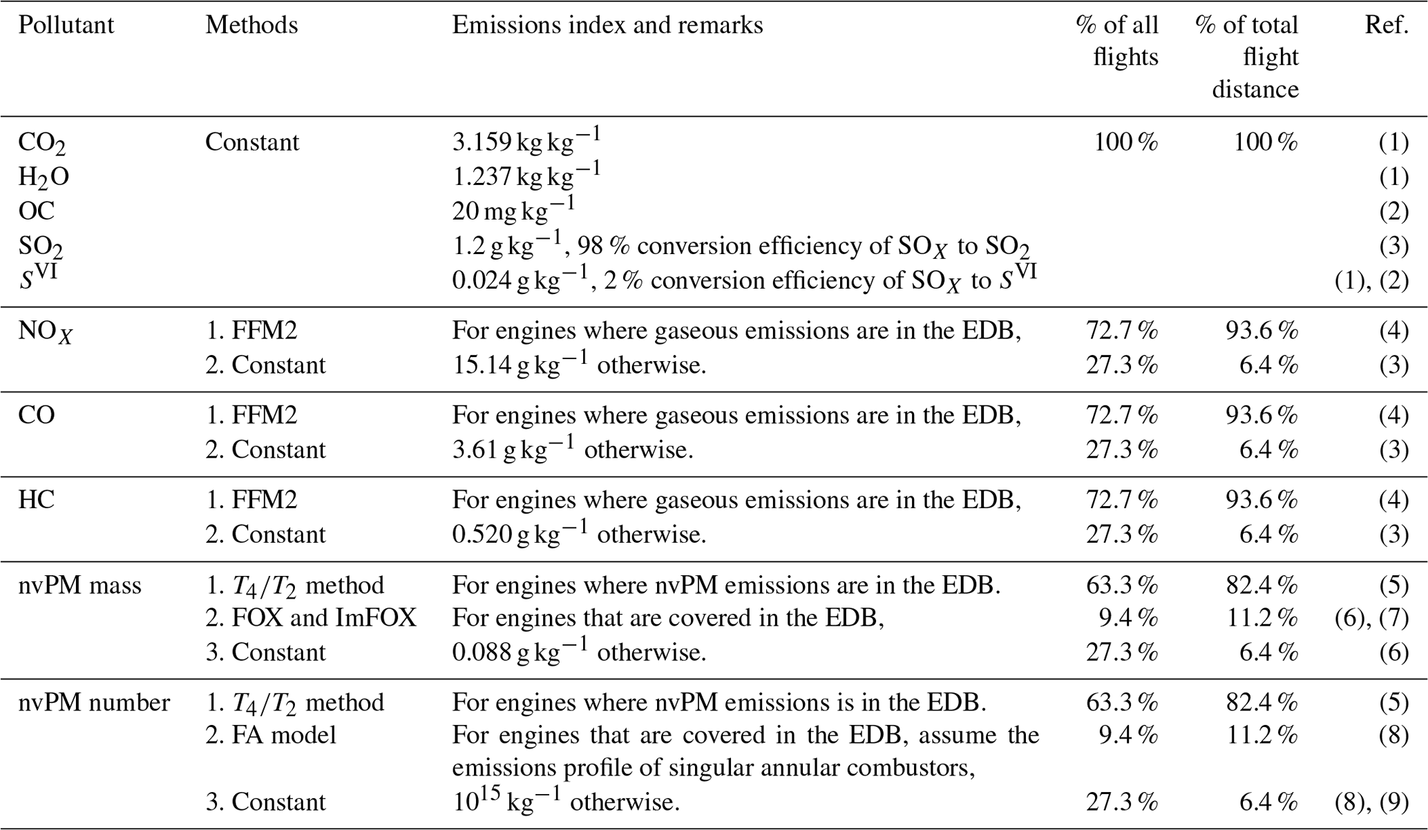
(1) Wilkerson et al. (2010); (2) Stettler et al. (2011); (3) Lee et al. (2021); (4) DuBois and Paynter (2006); (5) Teoh et al. (2022); (6) Stettler et al. (2013); (7) Abrahamson et al. (2016); (8) Teoh et al. (2020); (9) Schumann et al. (2015).
The EIs for NOX, CO and HC vary with engine-operating conditions and combustor type and are estimated using (i) the Fuel Flow Method 2 (FFM2) (DuBois and Paynter, 2006) when a gaseous EI for the specific engine type is provided by the ICAO EDB (EASA, 2021) (available for 557 unique engine types, covering 72.7 % of all flights and 93.6 % of the flight distance in the ADS-B dataset) or (ii) a constant EI that is representative of the historical fleet-average values (Wilkerson et al., 2010) when engine-specific EI data are not available (27.3 % of all flights, of which 91 % of these are flights flown by turboprop and piston aircraft). The NOX EI is sensitive to the ambient humidity, and a humid atmosphere can suppress engine NOX production (DuBois and Paynter, 2006). While the FFM2 assumes a fixed relative humidity of 60 % for all waypoints, we use humidity data from the ERA5 HRES at each waypoint. We also highlight that the engine-specific NOX EI in the ICAO EDB is reported as an NO2 mass equivalent (ICAO, 2017). For future studies that require cruise NOX emissions to be broken down into individual species, references can be made to previous in situ measurements which assume the engine exit NO2 NOX and NO NOX molar mixing ratios to have global means of 0.07 and 0.93 respectively (Schulte et al., 1997) and the nitrous acid (HONO) EI to be 0.31 g per kilogram NO2 (Jurkat et al., 2011). For the landing and take-off (LTO) cycle, existing studies have estimated that the NO2 NOX molar mixing ratio varies significantly based on engine type and thrust settings and ranges between (i) 0.05 and 0.10 during climb and take-off, (ii) between 0.12 and 0.20 during the descent phase and (iii) between 0.75 and 0.98 during the taxi phase (Timko et al., 2010; Wood et al., 2008; Wey et al., 2006; Stettler et al., 2011).
The emissions profiles for the nvPM EIm and EIn are unique for different engine combustor type and power settings and can vary by up to 5 orders of magnitude (EASA, 2021; Teoh et al., 2022). Since December-2020, the ICAO EDB has reported the nvPM EIm and EIn for all in-production and new turbofan engines with rated thrusts above 26.7 kN, covering 178 unique engine types (ICAO, 2022; EASA, 2021). We use the nvPM EIs that are corrected for dilution, thermophoretic and particle line losses (EASA, 2020). For aircraft-engine types with nvPM measurements (63.3 % of all flights and 82.4 % of the total flight distance), the nvPM EIm and EIn are estimated by linear interpolation relative to the ratio of turbine inlet to compressor inlet temperatures (), a non-dimensional measure of engine thrust settings that captures the differences in engine-operating conditions at ground and cruise (Cumpsty and Heyes, 2015). The methodology, originally developed by Teoh et al. (2022), is improved and evaluated with ground and cruise nvPM EIn measurements from the ECLIF II/ND-MAX (Emission and CLimate Impact of alternative Fuels 2 and the NASA/DLR-Multidisciplinary Airborne eXperiments) experimental campaign (Schripp et al., 2022; Bräuer et al., 2021; Voigt et al., 2021) (Supplement Sect. S4.1). For older aircraft-engine types where nvPM is not reported in the ICAO EDB (9.4 % of flights and 11.2 % of the flight distance), we estimate the nvPM according to Teoh et al. (2020): the EIm is estimated by using an average of the formation and oxidation (FOX) (Stettler et al., 2013) and improved FOX methods (Abrahamson et al., 2016), assuming the emissions profile of singular annular combustors; and the fractal aggregates model is used to convert the estimated EIm to EIn (Teoh et al., 2019, 2020) (Supplement Sect. S4.2). For the remaining flights without engine-specific data, the nvPM EIm and EIn are set to constant values of 0.088 g kg−1 and 1015 kg−1 respectively, which are nominal fleet-average values reported in earlier studies (Stettler et al., 2013; Schumann et al., 2015; Teoh et al., 2020).
2.4 Global aviation emissions inventory
GAIA is processed in three formats: (i) flight-waypoint outputs containing the fuel consumption and emissions at each waypoint; (ii) flight-summary outputs, which contain the metadata (flight identifier, mission profile and aircraft-engine characteristics) and aggregate the fuel consumption and emissions for each flight; and (iii) gridded outputs that aggregate the flight-waypoint outputs to a 4D grid of up to 0.5∘ × 0.5∘ horizontal resolution, at 100 m altitude intervals and at a 1 h temporal resolution. These different outputs will allow GAIA to be used as inputs to different climate models, such as Lagrangian-based models that use flight-waypoint data (Schumann, 2012; Schumann et al., 2012; Caiazzo et al., 2017; Fritz et al., 2020) and general circulation models that work with gridded inputs (Olsen et al., 2013b; Chen and Gettelman, 2013; Burkhardt and Kärcher, 2011; Bock and Burkhardt, 2019). Here, the flight-waypoint outputs are used to compute statistics on the routing inefficiencies and distribution of aviation emissions by mission profiles, while rectangular spatial bounding boxes are applied to the gridded outputs to estimate the aviation emissions from different world regions (Fig. 1 and Table 2). We note that GAIA only captures the fuel consumption and emissions after the flight is airborne and hence does not account for ground emissions during taxi, during take-off and from the use of auxiliary power units (APUs).
Table 2Spatial bounding boxes used to estimate the regional aviation activity and emissions.
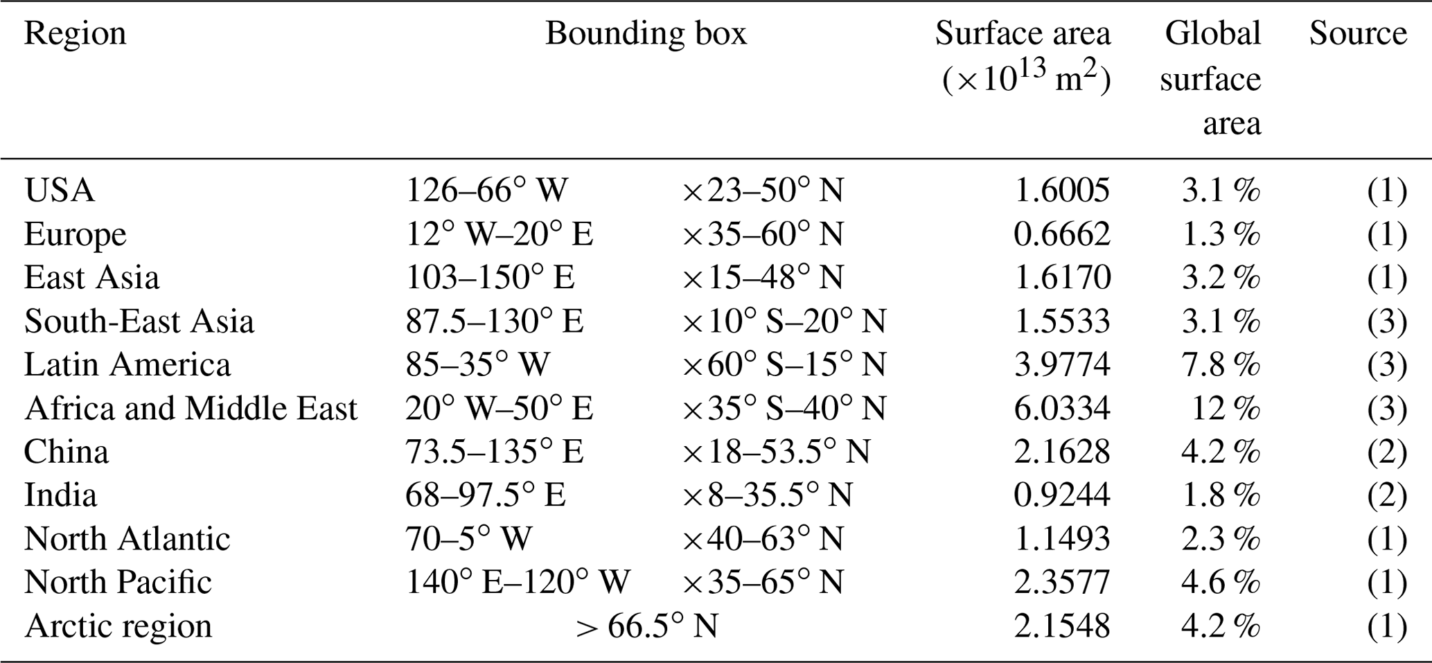
(1) Wilkerson et al. (2010); (2) Hoare (2014); (3) defined in this study.

Figure 1Spatial bounding boxes of the key regions of interest that are used to estimate the regional aviation activity and emissions. The specific dimensions of the bounding boxes are listed in Table 2. Basemap plotted using Cartopy 0.21.1 Natural Earth; license: public domain.
We first present the annual air traffic activity and emissions for 2019 (Sect. 3.1), which is used as a base year to represent normal traffic conditions, followed by quantifying the impacts of COVID-19 on aviation (Sect. 3.2). Table 3 summarises the global air traffic activity, fuel consumption and emissions from 2019 to 2021. These annual statistics are then compared with existing studies (Sect. 3.3), followed by an evaluation of granular statistics from individual flights (Sect. 3.4).
Table 3Annual statistics on the global aviation activity, fuel burn and emissions from 2019 to 2021.
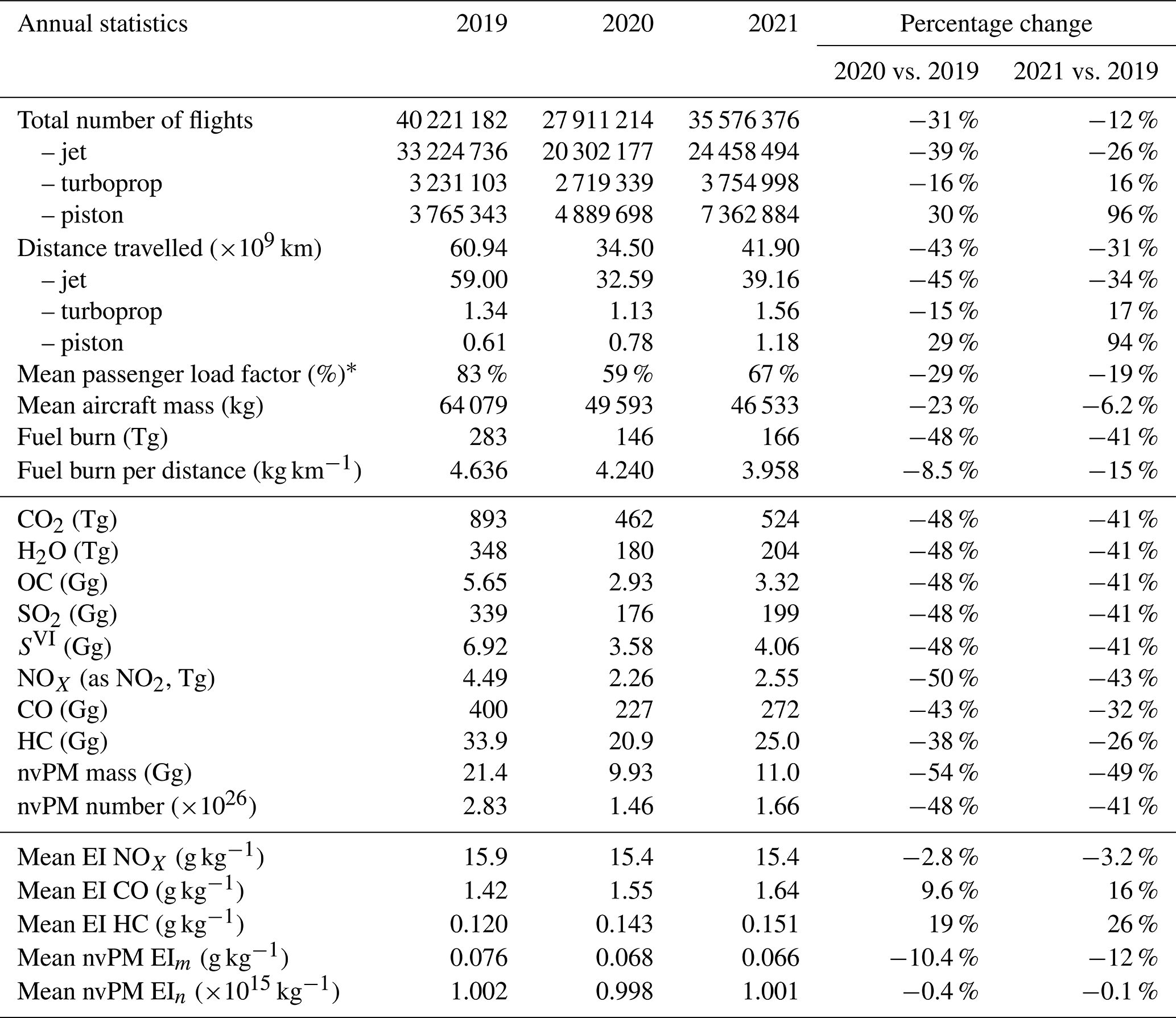
* The passenger load factor for each flight was derived using the global and regional data published by ICAO and IATA (refer to Sect. 2.2 and Supplement Sect. S3).
3.1 Annual statistics: 2019
In 2019, there are 40 221 182 unique flights recorded in the ADS-B dataset (83 % by jet aircraft, 8 % by turboprop and 9 % by piston aircraft), and the annual flight distance travelled amounts to 60.9 × 10⁹ km (97 % by jet aircraft, 2 % by turboprop and 1 % by piston aircraft). Figure 2a shows the 2019 global air traffic density, defined as the total flight distance flown divided by the regional surface area and time; 92 % of the annual flight distance flown occurred in the Northern Hemisphere and 63 % in the northern mid-latitudes (30–60∘ N). There were small amounts of flight distance flown in the Arctic Circle above 66.5∘ N (0.62 %) and below 45∘ S (0.06 %). On a regional level, Europe, USA and East Asia, which cover 7.6 % of the global surface area, had the highest air traffic densities (means of 0.152, 0.116 and 0.059 km−1 h−1 respectively) and are responsible for a total of 55 % of the global annual flight distance flown (Table 4). The North Atlantic (0.030 km−1 h−1) and North Pacific flight corridors (0.012 km−1 h−1) account for 4.9 % and 3.9 % respectively of the annual distance travelled, while 52 % of the globe has an air traffic density below 0.001 km−1 h−1.
Global aviation consumed 283 Tg of fuel in 2019, of which ∼ 92 % was burned in the Northern Hemisphere (Fig. S13b) and ∼ 79 % above 25 000 ft ( 7.6 km) (Fig. 3a). Air traffic activity within the spatial bounding boxes of the US, Europe and East Asia accounted for 47 % of the annual fuel consumption (Table 4). There are notable differences in the regional distribution of fuel consumption relative to the air traffic density. The proportion of fuel consumption in the US (19 %) is lower than its share of aviation activity (27 % of the global annual flight distance flown), and the mean fuel consumption per distance flown (3.29 kg km−1) is 29 % lower than the global average (4.64 kg km−1) (Fig. 4 and Table 4). In contrast, the North Atlantic and North Pacific flight corridors have a higher share of fuel consumption (13 %) than their distance flown (8.8 %), and the mean distance-specific fuel consumption (6.61 kg km−1) is 43 % higher than the global average (Fig. 4 and Table 4). The discrepancies in distance-specific fuel consumption are due to a higher proportion of short-haul domestic flights in the US predominantly served by smaller narrow-body aircraft, while larger and heavier wide-body aircraft are generally used for long-haul transoceanic flights. We note that the distance-specific fuel consumption in China (4.99 kg km−1) is 52 % and 21 % higher than the US (3.29 kg km−1) and Europe (4.14 kg km−1) respectively, and this could be due to the difference in (i) airspace structure (Rosenow et al., 2022; IFALPA, 2008), which likely caused a higher proportion of flights in Chinese airspace to cruise at lower altitudes of between 25 000 (7.6 km) and 35 000 ft (10.7 km) (44 % of the total flight distance flown) relative to other regions (31 % of the flight distance flown globally) (Fig. S14); and (ii) fleet composition mix (narrow- or wide-body aircraft). Global aviation emissions of CO2 (893 Tg in 2019), H2O (348 Tg), OC (5.65 Gg), SO2 (339 Gg) and SVI (6.92 Gg) are calculated with a constant EI and therefore have the same spatial distribution relative to fuel consumption. The emissions of NOX (4.49 Tg), CO (400 Gg), HC (33.9 Gg) and nvPM mass (21.4 Gg) and number (2.83 × 1026) depend on engine-operating conditions and ambient meteorology. Around 76 % of annual NOX emissions were emitted above 25 000 ft (7.6 km), while the proportions of CO (∼ 48 %) and HC (∼ 55 %) emitted at cruise are notably lower than the fuel consumption (∼ 79 %) because these pollutants generally have lower EIs at high engine thrust settings (DuBois and Paynter, 2006; Durdina et al., 2017; EASA, 2021; Lobo et al., 2015; Boies et al., 2015) (Fig. 3). At altitudes above 45 000 ft (13.7 km), the mean nvPM EIm (0.39 g kg−1) and EIn (4.5 × 10¹⁵ kg−1) are around 4–5 times larger than the global mean values (0.076 g kg−1 and 1.0 × 10¹⁵ kg−1) (Fig. 3b). This phenomenon can be attributed to a higher prevalence of private business jets with large nvPM EIm and EIn of up to 0.58 g kg−1 and 7 × 10¹⁵ kg−1 respectively (Table S8). The mean EIs of CO, HC, nvPM EIm and EIn in high air traffic density regions (US and Europe) are ∼ 30 % larger than the global average because of a higher proportion of the flight segments in descent, while these EIs are ∼ 36 % smaller than the global average over the oceans (North Atlantic and North Pacific) because the engines generally operate at higher thrust settings at cruise (Fig. 4 and Table 4).
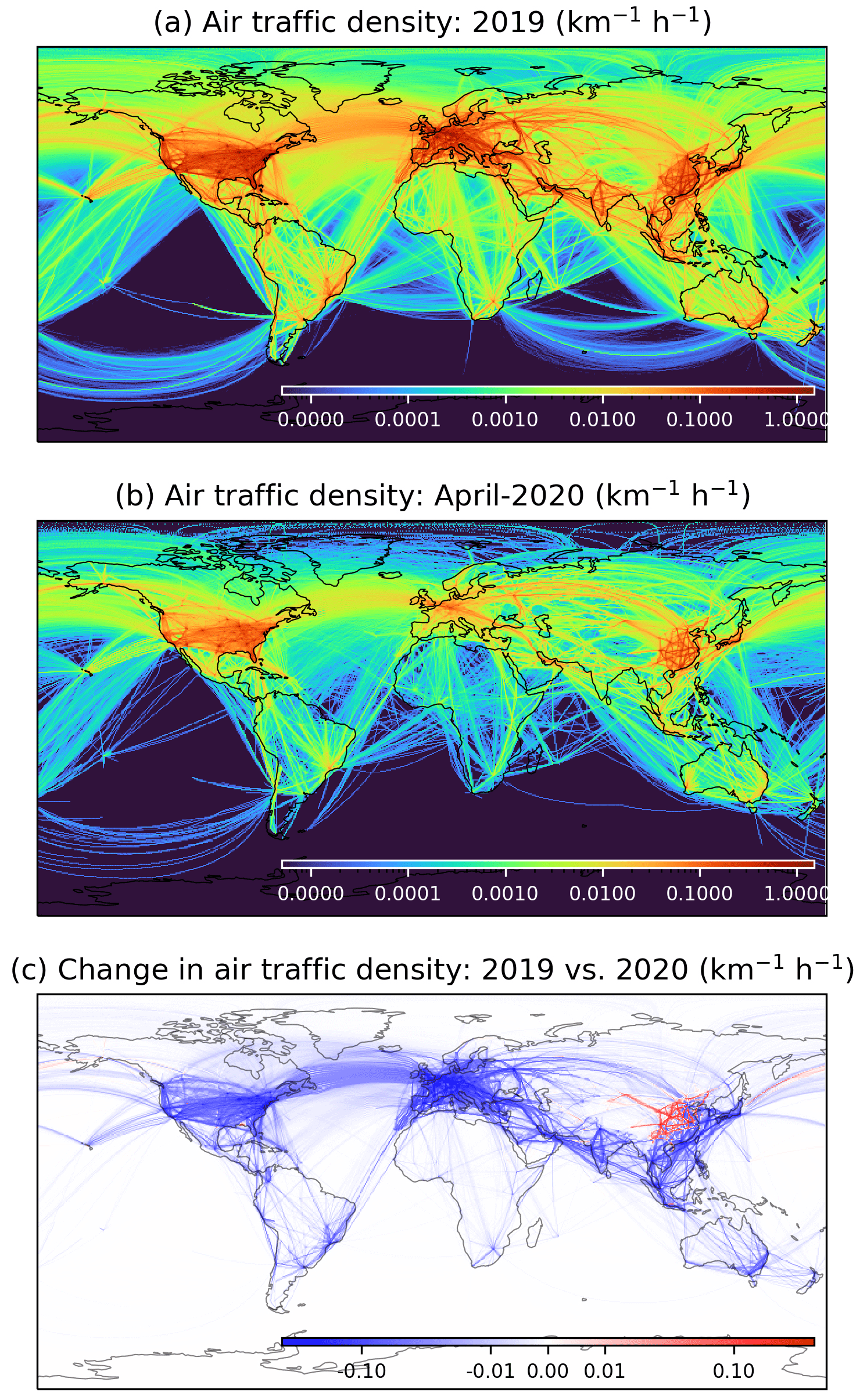
Figure 2The global (a) annual air traffic density in 2019. (b) Monthly air traffic density in April-2020, where air traffic activity was at a minimum due to the COVID-19 pandemic. (c) The change in annual air traffic density between 2019 and 2020. Basemap plotted using Cartopy 0.21.1 Natural Earth; license: public domain.
3.2 Impacts from COVID-19
COVID-19 led to significant reductions in global air traffic activity. The total flight distance travelled reached a minimum in April 2020 (−76 % globally relative to April 2019, shown in Fig. 2b), and the annual flight distances flown in 2020 and 2021 are 43 % and 31 % lower than in 2019 respectively (Table 3). Figure 2c compares the change in air traffic density between 2019 and 2020 and shows significant regional variability: the largest year-on-year reduction in the flight distance travelled was observed in the North Atlantic (−61 %), South-East Asia (−61 %) and Europe (−59 %) regions, which have a higher proportion of international flights, followed by Africa and the Middle East (−57 %), Latin America (−52 %), the North Pacific (−33 %), the USA (−31 %) and East Asia (−24 %). East China (25–42∘ N, 100–118∘ E) is the only region that recorded air traffic growth in 2020 compared with 2019 (+21 %).
Table 4Regional aviation activity, fuel consumption and emissions for 2019. The statistics for 2020 and 2021 can be found in Tables S9 and S10 (Supplement Sect. S5).
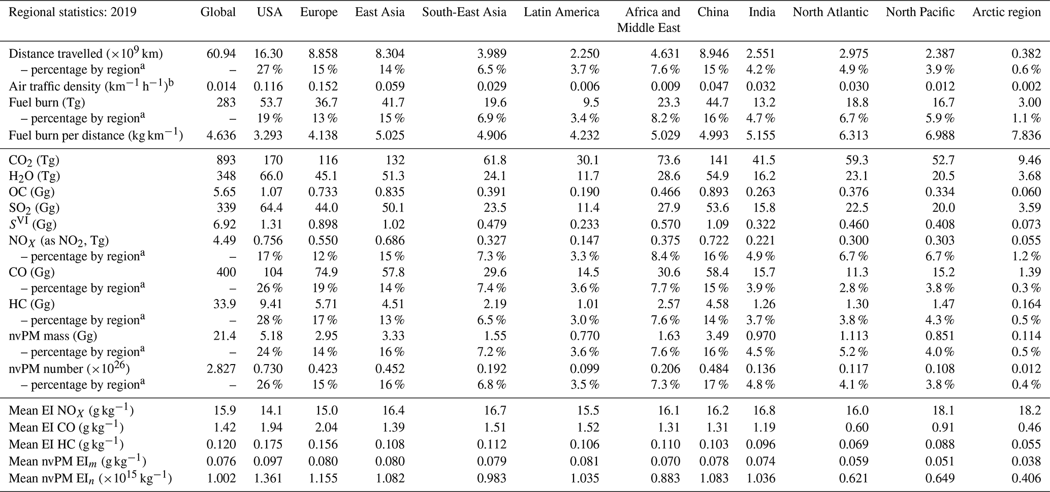
a The percentages of each region do not add up to 100 % because there is some overlap between the regional bounding boxes. When taken together, these regions do not cover 100 % of Earth's surface area (refer to Fig. 1 and Table 2). b The air traffic density (ATD) is defined as the total flight distance flown in the region divided by its surface area and time: ATD (km−1 h−1) = .
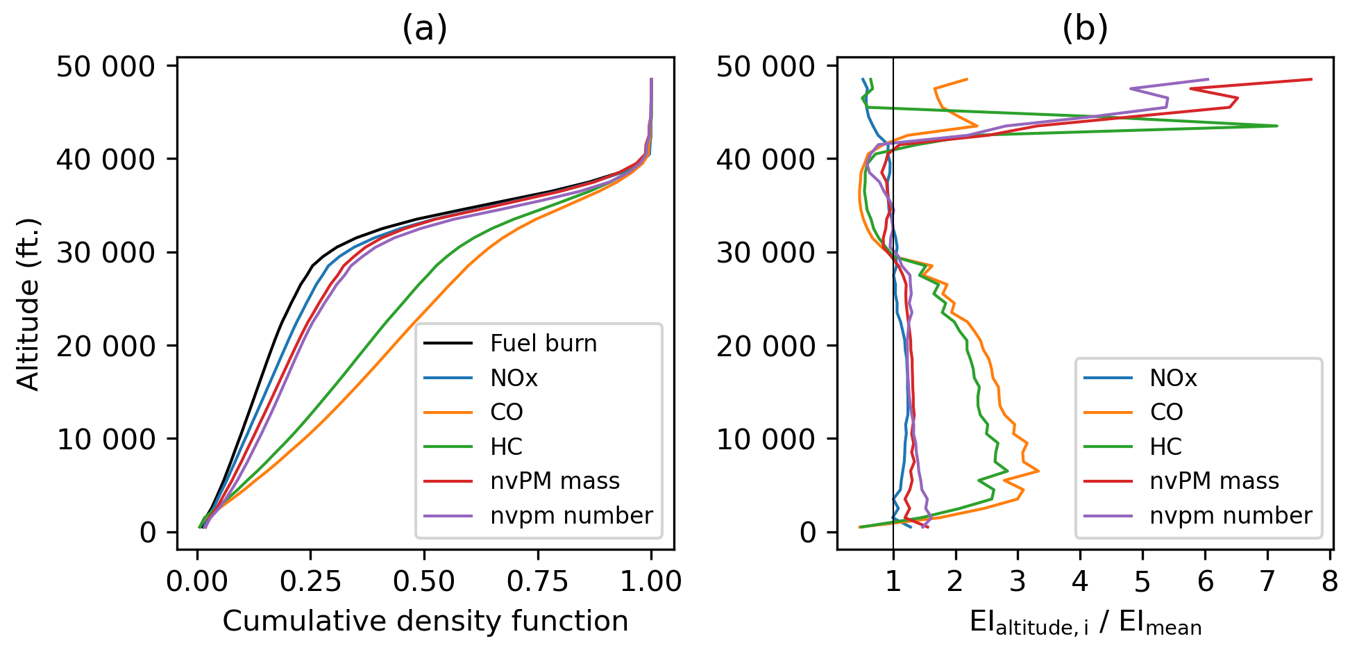
Figure 3(a) Cumulative density function of the 2019 annual fuel burn by altitude. (b) The ratio of the mean emission indices (EIs) at different altitudes relative to their respective global mean EIs. For both figures, NOX is denoted in blue, CO in orange, HCs in green), nvPM mass in red and nvPM number in purple.
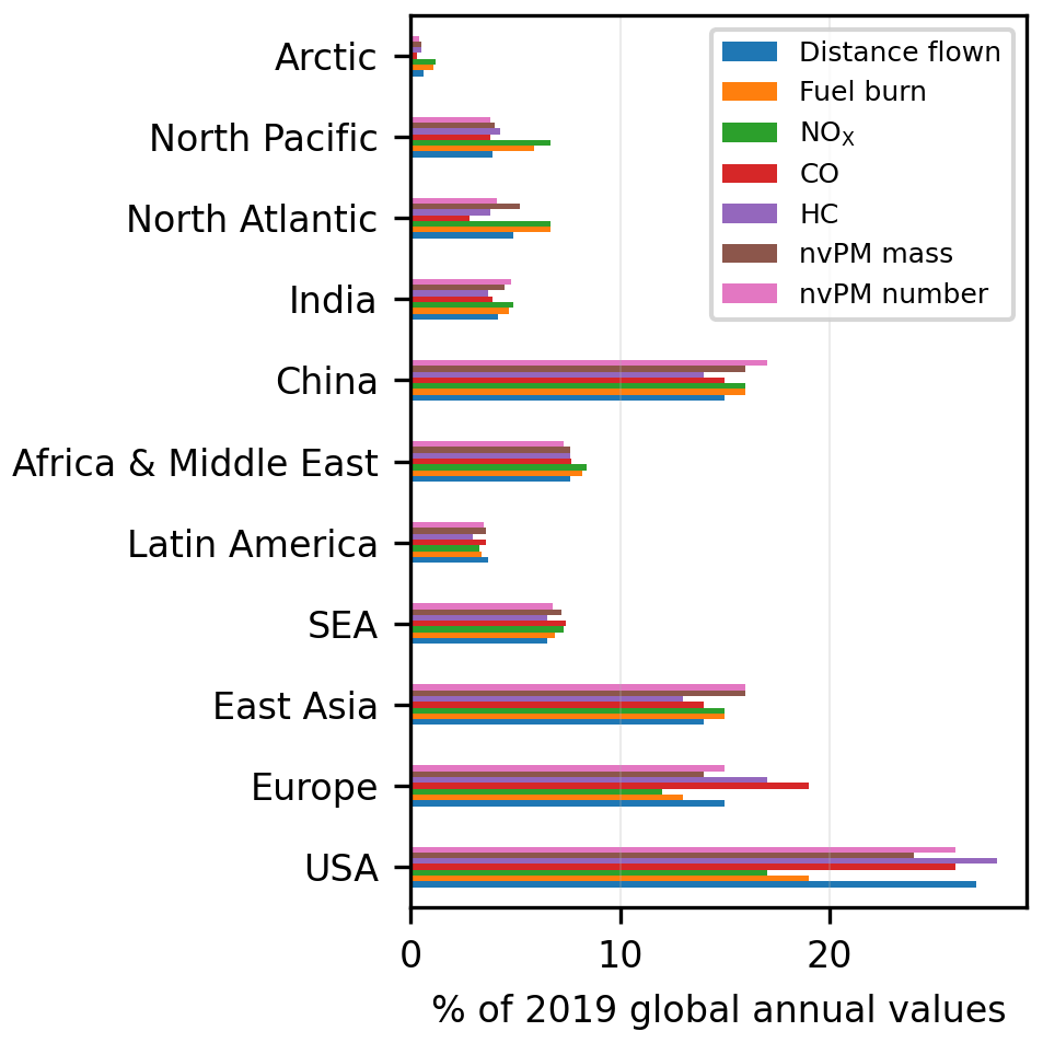
Figure 4Percentage breakdown of the 2019 global annual flight distance flown, fuel consumption, NOX, CO, HC, nvPM mass and number emissions by region.
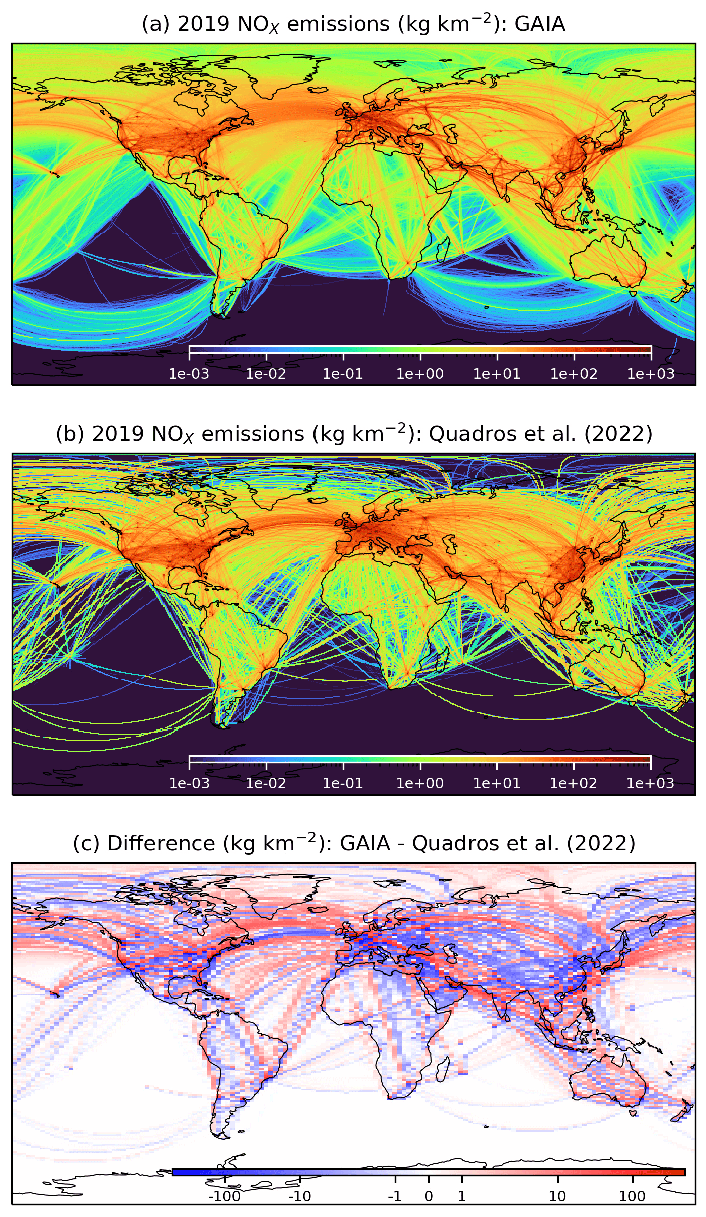
Figure 5Spatial distribution of the 2019 column-integrated NOX emissions from (a) GAIA with actual flight trajectories vs. (b) estimates from Quadros et al. (2022) which used monthly averaged flight trajectories. (c) The absolute difference in column-integrated NOX emissions between panels (a) and (b). Basemap plotted using Cartopy 0.21.1 Natural Earth; license: public domain.
Globally, reductions in the annual fuel consumption and CO2 emissions (−48 % in 2020 and −41 % in 2021 relative to 2019 levels) are greater than the change in flight distance travelled (−43 % and −31 % respectively), thereby causing the mean fuel consumption per flight distance flown in 2020 (4.24 kg km−1) and 2021 (3.96 kg km−1) to be 9 % and 15 % lower than 2019 levels (4.64 kg km−1) respectively (Table 3). The lower distance-specific fuel consumption is most likely caused by the lower global annual mean aircraft mass (−23 % in 2020 and −6.2 % in 2021 relative to 2019, Table 3), which in turn can be attributed to the (i) lower annual mean passenger load factor (59 % in 2020 and 67 % in 2021 vs. 83 % in 2019); (ii) reduction in long-haul flights (> 6 h) in 2020 and 2021 (3 % of all flights) relative to 2019 (5 % of all flights), where their mean aircraft mass is around 2–4 times larger than those of short- and medium-haul flights (< 6 h) generally flown by narrow-body aircraft (Tables 5, S11 and S12); and (iii) increased usage of private jets in the global fleet composition (Fig. S9). The change in aircraft fleet composition and mission profile during the COVID-19 pandemic also contributed to differences in the mean EIs of CO (+13 % relative to 2019), HC (+23 %), NOX (−3.0 %) and nvPM EIm (-12 %) (Table 3).
3.3 Comparison with other studies
GAIA's 2019 estimate of aviation's total fuel consumption (283 Tg) is 12 % lower than the IEA's top-down estimate of the global jet kerosene consumption (320 Tg) (IEA, 2020) and 4.7 % lower than bottom-up estimates from Quadros et al. (2022) (297 Tg, derived from Flightradar24 ADS-B telemetry). The incomplete coverage area of ADS-B receiver networks (Fig. S1) is likely one of the limitations causing the annual fuel consumption estimates from both GAIA and Quadros et al. (2022) to be lower than the IEA's top-down estimates. Several factors contribute to the differences in the annual fuel consumption between GAIA and Quadros et al. (2022): (i) fuel consumption from ground operations (i.e. taxi, take-off and use of APUs) is not included in GAIA; (ii) use of actual flight trajectories and meteorology in GAIA, which comes at a cost where ∼ 27 % of flights in 2019 have incomplete trajectories (i.e. waypoints do not begin and end at the origin and destination airports respectively) (Fig. S7d); and (iii) methodological differences where Quadros et al. (2022) used monthly averaged flight trajectories and wind fields and applied a constant scaling factor to account for routing inefficiencies (40.5 NM + 3.87 % of the great circle distance). The International Council on Clean Transportation (ICCT) inventory study estimates the 2019 annual CO2 emissions from all commercial operations to be 918 Tg (Graver et al., 2020), and our estimates (892 Tg of annual CO2 emissions from jet and turboprop aircraft) differ by 2.8 %. We also compare the relative change in global aviation CO2 emissions between 2019 and 2020, and our estimates are in good agreement with Quadros et al. (2022) (−48.2 % in this study vs. −47.1 %) and Liu et al. (2020) (−44.0 % vs. −43.9 % for the first half of 2020).
The 2019 mean EI NOX from GAIA (15.9 g kg−1) is within 2 % when compared with Quadros et al. (2022) (15.6 g kg−1). It is also 17 % and 11 % larger relative to the 2002 AERO2K (13.2 g kg−1) and 2006 AEDT (14.2 g kg−1) global aviation emissions inventories (Eyers et al., 2005; Wilkerson et al., 2010) respectively, which likely reflects the increasing use of more fuel-efficient engines that operate at higher combustion temperatures and pressures (Kyprianidis and Dahlquist, 2017; Freeman et al., 2018). The emissions profiles for NOX, CO, HC and nvPM vary for different aircraft-engine types (Figs. S18 to S22), and differences in the treatment of aircraft-engine combinations between our study and Quadros et al. (2022) could also contribute to discrepancies in the 2019 EI CO (1.4 g kg−1 from GAIA vs. 2.7 g kg−1, −48 %), HC (0.12 vs. 0.14 g kg−1, −14 %), nvPM EIm (76 mg kg−1 vs. 33 mg kg−1, +130 %) and EIn (1.00 vs. 1.17 × 10¹⁵ kg−1, −14.5 %). The significantly lower estimate of nvPM EIm from Quadros et al. (2022) (33 mg kg−1) relative to this study (76 mg kg−1) could also be attributed to their use of the Döpelheuer and Lecht relation to scale the nvPM emissions from the ground to cruising altitudes (Peck et al., 2013; Döpelheuer and Lecht, 1998), which was developed based on a limited number of cruise measurements and could underestimate the nvPM EIm (Abrahamson et al., 2016).
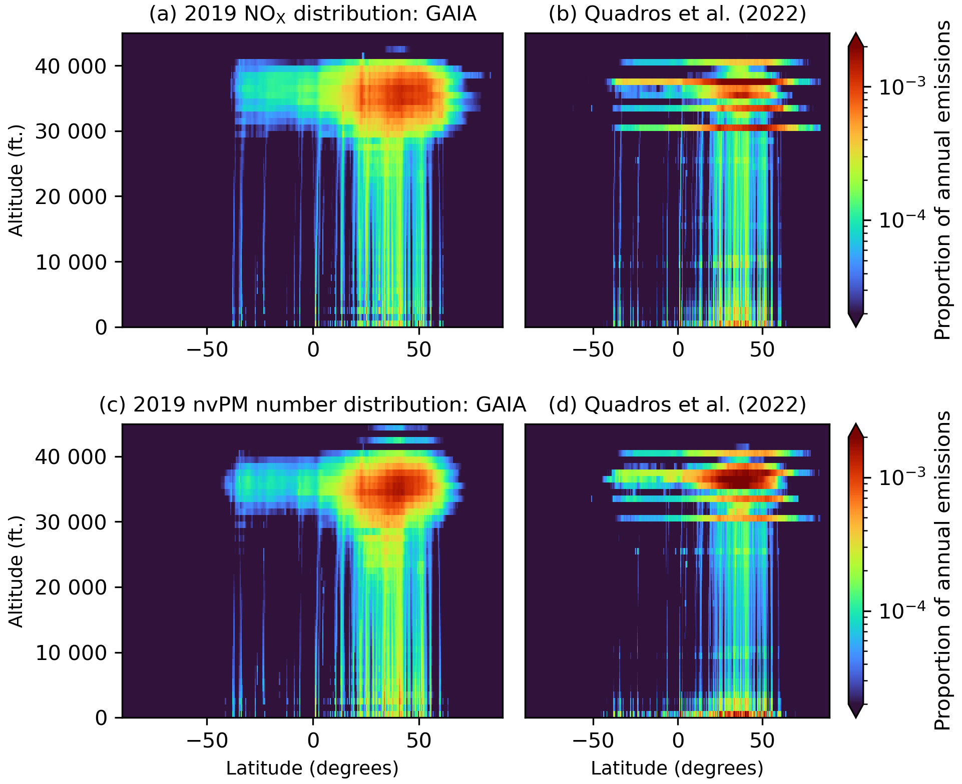
Figure 6Distribution of the 2019 NOX and nvPM number emissions by latitude and altitude from GAIA with actual flight trajectories (subplots a and c) vs. estimates from Quadros et al. (2022) with monthly averaged flight trajectories (subplots b and d). The colour bar represents the proportion of annual emissions, i.e. annual emissions at each grid cell divided by the global annual emissions, where the summation of values across all grid cells would be equal to 1.
Notably, there are significant differences in the spatial distribution of global aviation emissions between GAIA and Quadros et al. (2022) (Figs. 5, 6 and S16): the use of actual flight trajectories in GAIA caused the fuel consumption and pollutants to be more spatially dispersed, while Quadros et al. (2022) used monthly averaged flight trajectories, resulting in emissions that are more concentrated along established flight corridors and selected altitudes. The air traffic activity in GAIA is also more representative of real-world operations, where aircraft actively avoid flying over the Himalayas, Tibet and conflict zones (Safe Airspace, 2022) (i.e. Ukraine, Syria, Yemen, Libya and North Korea) (Figs. 5 and S16).
3.4 Flight-level statistics
We categorise the 2019 global air traffic activity into three groups based on their flight durations (Wilkerson et al., 2010), consisting of short- (t≤3 h), medium- (3 < t < 6 h) and long-haul (t > 6 h) flights (Table 5). In 2019, short-haul flights (83 % of all flights and 49 % of the total distance travelled) accounted for 35 % of the total CO2 emissions and the largest fractions of CO (59 %), HC (52 %) and nvPM mass (45 %) and number (51 %) emissions because a greater proportion of flight time is in descent where the EIs of these pollutants are generally at their maximum (Figs. S19 to S22). In contrast, long-haul flights (5 % of all flights and 26 % of the distance travelled) are responsible for the largest shares of CO2 (43 %) and NOX (49 %) emissions because of the significantly larger mean aircraft mass (∼ 3.5 times greater than short-haul flights) that can be attributed to the use of the larger wide-body aircraft and higher fuel mass fraction (∼ 26 % of the initial aircraft mass vs. ∼ 6 % for short-haul flights) (Table 5 and Fig. S9d). Travel restrictions due to COVID-19 caused the proportion of international flights to decrease from 39 % (2019) to 23 % (2020 and 2021). As a result, the share of short-haul flights increased from 83 % to 88 %, while that of long-haul flights decreased from 5 % to 3 %.
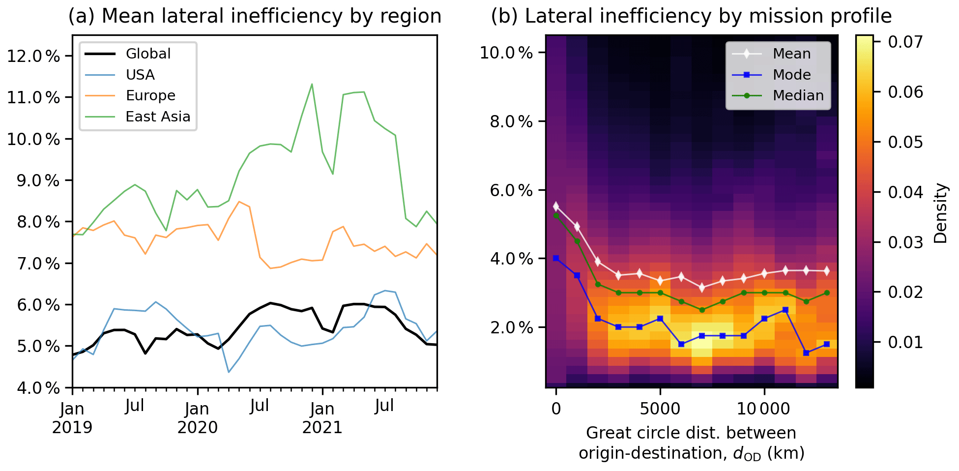
Figure 7The (a) mean lateral inefficiency of flights in different spatial domains (global, USA, Europe and East Asia) and the (b) distribution of lateral inefficiency when flights are categorised by their mission profile, defined by the great circle distance between their respective origin and destination airports. These statistics exclude the 1.5 % of flights where their erroneous trajectories were replaced with the great circle path between the origin and destination airports (Supplement Sect. S1.2).
Table 5Breakdown of aviation activity, fuel consumption and emissions for 2019 by flight duration. The statistics for 2020 and 2021 can be found in Tables S11 and S12 (Supplement Sect. S5).
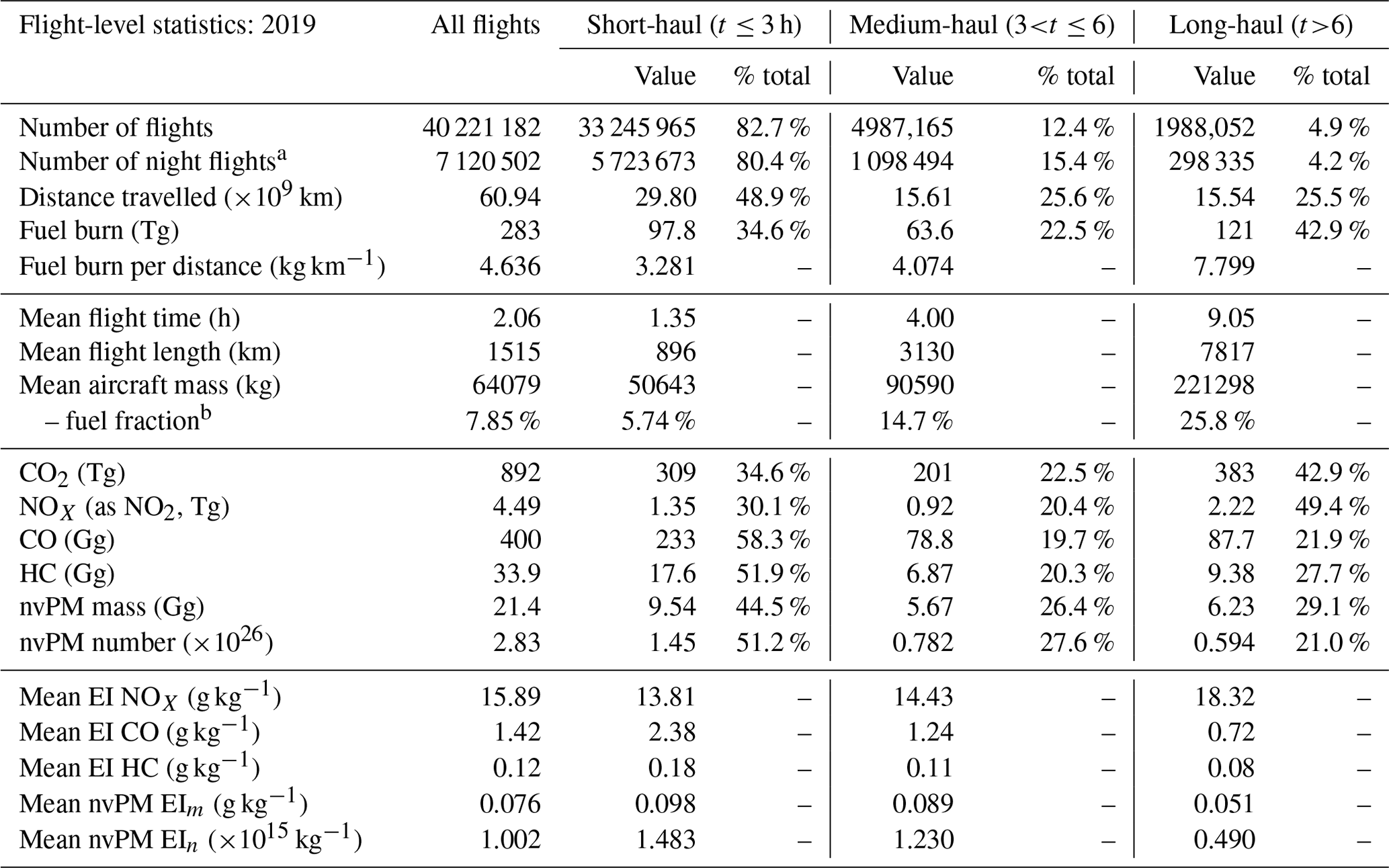
a Night flights are identified when their mean solar direct radiation (SDR) throughout their flight trajectory is < 1 W m−2. b Fuel fraction is the total fuel mass divided by the initial aircraft mass.
The global mean lateral route inefficiency, i.e. the additional distance flown relative to the great circle distance between the origin and destination airports (dOD), increased from 5.2 % in 2019 to 5.6 % in 2020–2021 with regional variations (Fig. 7a): reductions in air traffic levels due to COVID-19 likely led to small improvements in the mean lateral inefficiency in the US (5.5 % in 2019 vs. 5.1 % in 2020) and Europe (7.7 % vs. 7.5 %), while an increase in the lateral inefficiency in East Asia (from 8.3 % to 9.5 %) is likely caused by the air traffic growth experienced in China (Fig. 2c). Flights in East Asia and China tend to follow pre-defined air traffic corridors relative to a more direct routing in the US (Fig. 2) because around ∼ 70 % of the eastern Chinese airspace is restricted for military usage compared with ∼ 15 % in the US (Rosenow et al., 2022), and this is likely the primary factor causing the mean lateral inefficiency in East Asia (9.1 %) to be around 2 times higher than the US (5.4 %). Our estimate of the mean lateral inefficiency in Europe (∼ 7.5 %) is around 2 times larger than the official statistics from the European Organisation for the Safety of Air Navigation, EUROCONTROL (2022) (∼ 4 %), because the latter computes the lateral inefficiency relative to the shortest constraint route (i.e. constraints imposed by the airspace structure and availability) instead of the great circle distance. Given the significant regional variability in the lateral inefficiency factor, earlier studies that assume a constant lateral inefficiency factor of around 4 %–6 % could (i) underestimate the total distance travelled for flights outside the US and (ii) overestimate the flight distance for medium- and long-haul flights (Simone et al., 2013; Quadros et al., 2022).
We group each flight in 2019 by its origin–destination (OD) airport pair to evaluate the differences in their mean: (i) historical flight distance flown (dGAIA) vs. dOD; and (ii) simulated fuel consumption from GAIA (fGAIA) vs. the fuel consumption from the great circle trajectory that is estimated from the European Environment Agency emissions calculator (fEEA,OD), where fEEA,OD at the climb, cruise and descent (CCD) phase for each flight is estimated as a function of dOD and aircraft type (European Environment Agency, 2019). These OD statistics have been made open-source and are available as described in the “Data availability” section. In general, there is an inverse relationship between the lateral inefficiency and dOD, where the mean lateral inefficiency is 5.1 [0.7, 10.8] % (5th and 95th percentiles) for flights with dOD< 1000 km, 4.4 [0.9, 10.2] % when dOD is between 1000 and 2000 km and 2.9 [0.8, 8.6] % for dOD > 2000 km (Figs. 7b and 8a). Our analysis of OD airport pairs also suggests that (i) the variability of (1.14 [0.997, 1.35]) is greater than (1.06 [1.01, 1.16]) (Fig. S15); (ii) is relatively symmetrical between OD airport pairs irrespective of the direction travelled (Fig. 8a); and (iii) there is a directional bias in among OD airport pairs, e.g. westbound transatlantic flights consuming more fuel than eastbound transatlantic flights (Fig. 8b), because fGAIA captures the effects of ambient wind patterns.
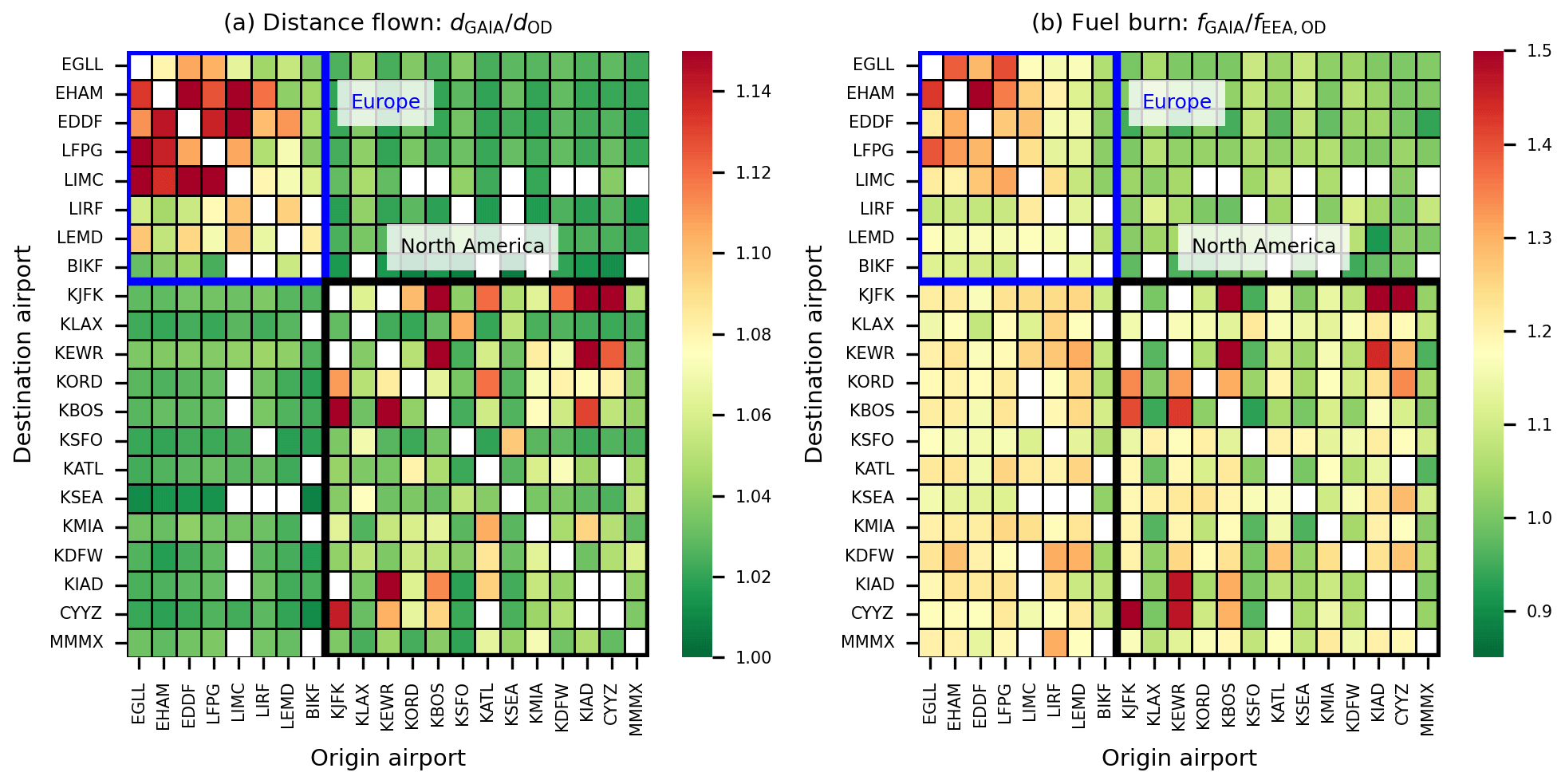
Figure 8The mean ratio of (a) the actual flight distance flown from GAIA over the great circle distance () and (b) the simulated fuel consumption from GAIA over the estimated fuel consumption from the great circle trajectory () across all flights that traversed between major European and North American airport pairs in 2019.
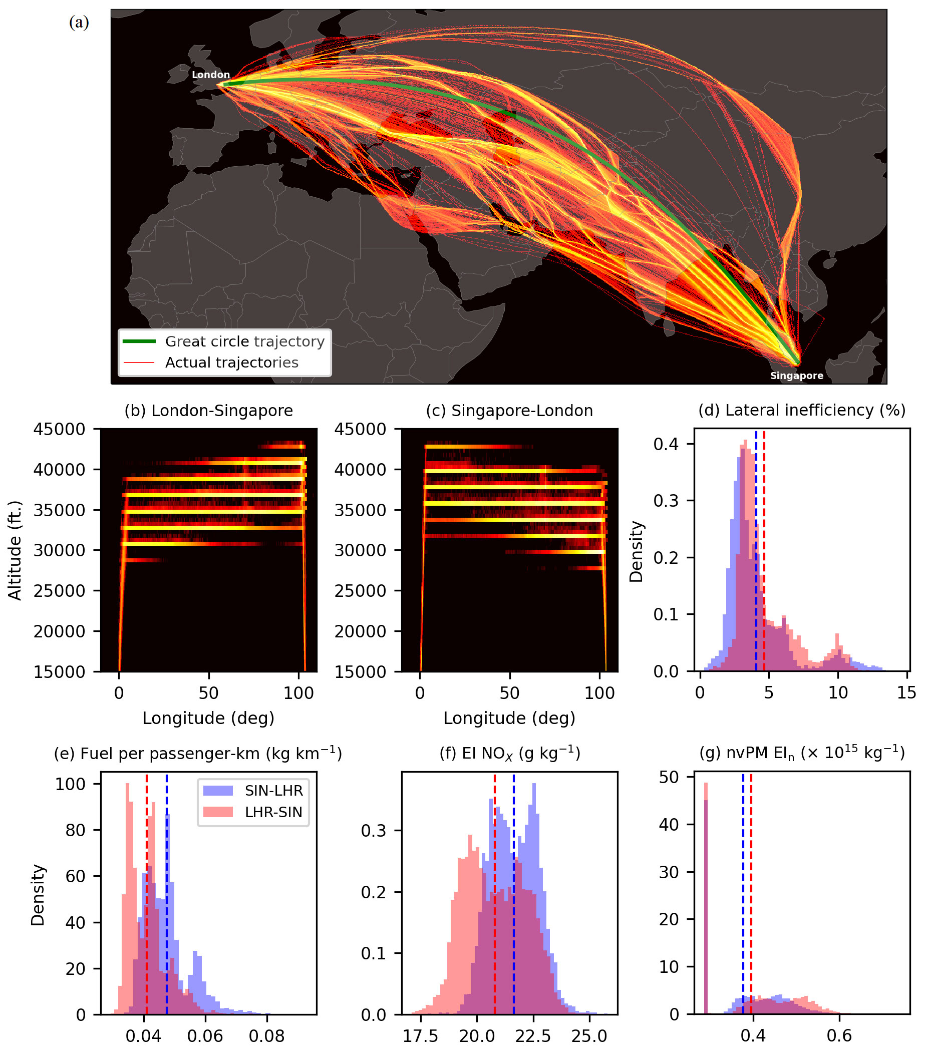
Figure 9The (a) lateral and (b–c) vertical trajectories that were flown by flights between London Heathrow Airport (LHR) and Singapore Changi Airport (SIN) between 2019 and 2021 (n = 8705). Probability density function of the (d) lateral inefficiency, (e) fuel consumption per passenger kilometre, (f) EI NOX and (g) nvPM EIn for westbound (SIN–LHR, in blue) and eastbound flights (LHR–SIN, in red). The methodology to estimate the fuel consumption per passenger kilometre is described in Supplement Sect. S5.2. Basemap plotted using Cartopy 0.21.1 Natural Earth; license: public domain.
Figure 9 shows the distribution in the flight trajectory, fuel consumption and emissions for trips between London Heathrow (LHR) and Singapore Changi Airport (SIN). There are large variabilities in the (i) flight trajectory profile, where the lateral inefficiency and cruising altitudes range between 2.1 % and 9.9 % (5th and 95th percentiles) and between 28 000 (8.5 km) and 42 000 ft (12.8 km) respectively; (ii) fuel consumption per passenger kilometre (0.03–0.06 kg km−1, 5th and 95th percentiles) arising from differences in aircraft type, passenger LF and wind conditions; and (iii) mean EI NOX (19.1–23.1 g kg−1) and nvPM EIn (2.9–5.4 × 10¹⁴ kg−1), which can be attributed to differences in engine combustor type, thrust settings and the ambient temperature and humidity. The mean fuel consumption per passenger kilometre for westbound flights (SIN–LHR: 0.047 kg km−1) is 15 % larger than eastbound flights (LHR–SIN: 0.041 kg km−1) because of the jet stream patterns that tend to flow from west to east. The difference in lateral inefficiency for SIN–LHR (4.1 [1.9, 10.0] %) vs. LHR–SIN (4.7 [2.7, 9.8] %) suggests that (i) eastbound flights tend to fly more consistent trajectories than westbound flights and that the route optimiser is less sensitive to the flight distance flown because of favourable jet stream conditions; while (ii) westbound flights have a larger variability in the distance flown, suggesting that flights are more actively re-routing where possible to avoid regions with the strongest headwinds. Westbound flights also tend to operate at higher engine thrust settings to counteract the effects of stronger headwinds, thereby leading to a larger mean EI NOX (+4.1 %) and lower nvPM EIn (−4.7 %) respectively relative to eastbound flights.
In this paper, we developed the high-resolution Global Aviation emissions Inventory based on ADS-B (GAIA) for 2019–2021 using (i) historical flight trajectories that are derived from ADS-B telemetry data collected by Spire Aviation; (ii) reanalysis weather data from the ECMWF ERA5 HRES; and (iii) existing datasets and methodologies to estimate the fuel consumption, CO2, NOX, CO, HC, OC, H2O, SO2, SVI and nvPM mass and number emissions for each flight. GAIA captures 103.7 million unique flights over 3 years, of which 75.2 % are completed using jet aircraft and the remainder by turboprop (9.4 %) and piston aircraft (15.4 %).
In 2019, there were ∼ 40.2 million flights that collectively consumed 283 Tg of fuel to travel 60.9 × 10⁹ km (mean distance-specific fuel consumption of 4.64 kg km−1), producing 893 Tg of CO2, 348 Tg of H2O, 5.7 Gg of OC, 339 Gg of SO2, 6.9 Gg of SVI, 4.5 Tg of NOX, 400 Gg of CO, 34 Gg of unburned HC, 21.4 Gg of nvPM mass and 2.8 × 1026 nvPM particles. Around 92 % of annual fuel consumption occurred in the Northern Hemisphere, and 79 % of it was burned at cruise altitudes above 25 000 ft ( 7.6 km). The United States, Europe and East Asia, covering ∼ 8 % of the global surface area, accounted for 47 % of the fuel consumption and CO2 emissions in 2019. Our estimated global annual fuel consumption for 2019 (283 Tg) is around 12 % smaller than top-down estimates from the IEA (320 Tg) and 5 % smaller than bottom-up estimates from Quadros et al. (2022) (297 Tg), which used monthly averaged flight trajectories and wind fields. Globally, COVID-19 led to significant reductions in the annual flight distance flown (−43 %) and fuel consumption (−48 %) in 2020, with the largest reductions occurring in the North Atlantic (−61 % in flight distance and −64 % in fuel consumption), South-East Asia (−61 % for both metrics) and Europe (−59 % and −60 % respectively), while East China recorded growth in both metrics (+21 % and +9 % respectively). In 2021, the global annual flight distance and fuel consumption remained 31 % and 41 % below 2019 levels.
An analysis of individual flight trajectories shows that 83 % of all flights in 2019 have durations below 3 h, and these short-haul flights only accounted for 35 % of the annual CO2 emissions. In contrast, only 5 % of all flights in 2019 are long-haul (duration > 6 h), but they have a disproportionate impact on the annual CO2 (43 %) and NOX (49 %) emissions. The mean lateral inefficiency increased from 5.2 % (2019) to 5.6 % (2020 and 2021) globally, and this is most likely due to a higher proportion of short-haul flights in 2020 and 2021 (∼ 88 % of all flights) relative to 2019 (83 %), which tend to have a higher routing inefficiency relative to long-haul flights (Fig. 7b). Regionally, there are small improvements in the mean lateral inefficiency over the US (from 5.5 % in 2019 to 5.1 % in 2020) and Europe (from 7.7 % to 7.5 %). In contrast, East Asia experienced an increase in mean lateral inefficiency (from 8.3 % in 2019 to 9.5 % in 2020), which is likely caused by the growth in air traffic over China. We evaluated 8649 unique flights between London and Singapore: the trajectories flown, fuel consumption, EI NOX and nvPM EIn showed large variabilities between flights, and the fuel consumption and emission indices between eastbound and westbound flights can differ by up to 15 %. By using flight trajectories that are representative of real-world operations, GAIA improves upon the spatiotemporal distribution of aviation emissions when compared with existing aviation emissions inventories. Future research can utilise GAIA to (i) quantify the climate impacts from aviation NOX emissions and contrail cirrus, whose radiative forcing has a strong spatiotemporal dependence; and (ii) perform inter-model comparison studies and uncertainty quantification of the climate impacts that arise from these aviation non-CO2 pollutants.
The following datasets are available at Zenodo: (i) low-resolution gridded outputs from GAIA for 2019–2021 (0.5∘ longitude × 0.5∘ latitude at altitude intervals of 100 m and at a monthly temporal resolution) (https://doi.org/10.5281/zenodo.7969631, Teoh et al., 2023c); (ii) high-resolution gridded outputs from GAIA (with a spatial resolution of up to 0.5∘ longitude × 0.5∘ latitude at altitude intervals of 100 m, and at an hourly temporal resolution) for the full year of 2019 (https://doi.org/10.5281/zenodo.8369829, Teoh et al., 2023a) and bi-monthly for 2020 and 2021 (https://doi.org/10.5281/zenodo.8369925, Teoh et al., 2023b); and (iii) lateral inefficiency and fuel consumption statistics on the origin–destination airport and country pairs for 2019 (https://doi.org/10.5281/zenodo.8369564, Teoh et al., 2023d). Flight trajectory and aircraft fuel consumption data are commercially sensitive, and the flight-waypoint and flight-summary outputs from GAIA can be made available for research purposes only upon reasonable request (m.stettler@imperial.ac.uk). This document used elements of Base of Aircraft Data (BADA) Family 4 Release 4.2, which has been made available by the European Organisation for the Safety of Air Navigation (EUROCONTROL) to Imperial College London. EUROCONTROL has all relevant rights to BADA © 2019. EUROCONTROL will not be liable for any direct, indirect, incidental or consequential damages arising out of or in connection with this document, including the use of BADA. This document contains Copernicus Climate Change Service information from 2022. Neither the European Commission nor the ECMWF is responsible for any use of the Copernicus information.
The supplement related to this article is available online at: https://doi.org/10.5194/acp-24-725-2024-supplement.
RT and MEJS conceptualised the study, developed the methodology, and undertook the investigation. MEJS and MS acquired the ADS-B air traffic dataset. LD acquired the fleet database. RT, ZE and MS were responsible for software development and data curation. RT and MEJS created or sourced the figures. RT wrote the original manuscript. RT, MS, LD and MEJS reviewed and edited the manuscript. MEJS and MS acquired funding. All the authors have read and agreed upon the published version of the paper.
The contact author has declared that none of the authors has any competing interests.
Publisher’s note: Copernicus Publications remains neutral with regard to jurisdictional claims made in the text, published maps, institutional affiliations, or any other geographical representation in this paper. While Copernicus Publications makes every effort to include appropriate place names, the final responsibility lies with the authors.
The authors thank Google for providing cloud credits on the Google Cloud Platform, which were utilised to produce the global aviation emissions inventory and the analysis of the results published in this paper. We thank Andreas Schäfer for his efforts in acquiring funding to purchase the fleet database and Thomas Dean for reviewing an earlier version of the paper. We thank the members of the German Aerospace Center (Christiane Voigt, Daniel Sauer and Tobias Schripp) for providing in situ measurements from the ECLIF II/ND-MAX experimental campaign which were used to improve the methodology to estimate the cruise nvPM emissions.
This paper was edited by Patrick Jöckel and reviewed by two anonymous referees.
Abrahamson, J. P., Zelina, J., Andac, M. G., and Vander Wal, R. L.: Predictive Model Development for Aviation Black Carbon Mass Emissions from Alternative and Conventional Fuels at Ground and Cruise, Environ. Sci. Technol., 50, 12048–12055, https://doi.org/10.1021/acs.est.6b03749, 2016.
Airbus: Airbus Global Market Forecast 2021–2040, https://www.airbus.com/sites/g/files/jlcbta136/files/2021-11/Airbus-Global-Market-Forecast-2021-2040.pdf (last access: 5 July 2022), 2021.
Airlines for America: World Airlines Traffic and Capacity, https://www.airlines.org/dataset/world-airlines-traffic-and-capacity/ (last access: 12 August 2022), 2022.
ATAG: Aviation: Benefits Beyond Borders, https://aviationbenefits.org/media/167517/aw-oct-final-atag_abbb-2020-publication-digital.pdf (last access: 12 August 2022), 2020.
Barrett, S. R. H., Britter, R. E., and Waitz, I. A.: Global mortality attributable to aircraft cruise emissions, Environ. Sci. Technol., 44, 7736–7742, https://doi.org/10.1021/es101325r, 2010.
Baughcum, S. L., Tritz, T. G., Henderson, S. C., and Pickett, D. C.: Scheduled Civil Aircraft Emissions Inventories for 1992: Database Development and Analysis, NASA CR 4700, 1996.
Bock, L. and Burkhardt, U.: Contrail cirrus radiative forcing for future air traffic, Atmos. Chem. Phys., 19, 8163–8174, https://doi.org/10.5194/acp-19-8163-2019, 2019.
Boeing: Commercial Market Outlook 2021–2040, https://www.boeing.com/resources/boeingdotcom/market/assets/downloads/CMO 2021 Report_13Sept21.pdf (last access: 5 July 2022), 2021.
Boies, A. M., Stettler, M. E. J., Swanson, J. J., Johnson, T. J., Olfert, J. S., Johnson, M., Eggersdorfer, M. L., Rindlisbacher, T., Wang, J., and Thomson, K.: Particle emission characteristics of a gas turbine with a double annular combustor, Aerosol Sci. Technol., 49, 842–855, https://doi.org/10.1080/02786826.2015.1078452, 2015.
Bond, T. C., Doherty, S. J., Fahey, D. W., Forster, P. M., Berntsen, T., DeAngelo, B. J., Flanner, M. G., Ghan, S., Kärcher, B., and Koch, D.: Bounding the role of black carbon in the climate system: A scientific assessment, J. Geophys. Res.-Atmos., 118, 5380–5552, https://doi.org/10.1002/jgrd.50171, 2013.
Bräuer, T., Voigt, C., Sauer, D., Kaufmann, S., Hahn, V., Scheibe, M., Schlager, H., Diskin, G. S., Nowak, J. B., DiGangi, J. P., Huber, F., Moore, R. H., and Anderson, B. E.: Airborne Measurements of Contrail Ice Properties – Dependence on Temperature and Humidity, Geophys. Res. Lett., 48, e2020GL092166, https://doi.org/10.1029/2020GL092166, 2021.
Burkhardt, U. and Kärcher, B.: Global radiative forcing from contrail cirrus, Nat. Clim. Change, 1, 54–58, https://doi.org/10.1038/nclimate1068, 2011.
Caiazzo, F., Agarwal, A., Speth, R. L., and Barrett, S. R. H.: Impact of biofuels on contrail warming, Environ. Res. Lett., 12, 114013, https://doi.org/10.1088/1748-9326/aa893b, 2017.
Chen, C. C. and Gettelman, A.: Simulated radiative forcing from contrails and contrail cirrus, Atmos. Chem. Phys., 13, 12525–12536, https://doi.org/10.5194/acp-13-12525-2013, 2013.
Cirium: Aircraft fleets and values: the world's largest independent aircraft database, https://www.cirium.com/solutions/fleets-and-valuations/ (last access: 30 November 2022), 2022.
Cumpsty, N. A. and Heyes, A.: Jet propulsion: A simple guide to the aerodynamics and thermodynamic design and performance of jet engines, 3nd Edn., Cambridge University Press, ISBN: 978-1107511224, https://doi.org/10.1017/CBO9781316223116, 2015.
Dalmau, R. and Prats, X.: Assessing the impact of relaxing cruise operations with a reduction of the minimum rate of climb and/or step climb heights, Aerosp. Sci. Technol., 70, 461–470, https://doi.org/10.1016/J.AST.2017.08.032, 2017.
Döpelheuer, A. and Lecht, M.: Influence of engine performance on emission characteristics, in: Symposium of the applied vehicle Technology Pane “Gas Turbine Engine Combustion, Emissions and alternative fuels”, Lisbon, Portugal, 12–16 October 1998, RTO MP-14, 1998.
DuBois, D. and Paynter, G.: Fuel Flow Method2 for Estimating Aircraft Emissions, J. Aerosp., 115, 1–14, https://doi.org/10.4271/2006-01-1987, 2006.
Durdina, L., Brem, B. T., Setyan, A., Siegerist, F., Rindlisbacher, T., and Wang, J.: Assessment of Particle Pollution from Jetliners: from Smoke Visibility to Nanoparticle Counting, Environ. Sci. Technol., 51, 3534–3541, https://doi.org/10.1021/acs.est.6b05801, 2017.
EASA: Implementation of the latest CAEP amendments to ICAO Annex 16, Vol. I, II and III, https://www.easa.europa.eu/sites/default/files/dfu/NPA 2020-06.pdf (last access: 5 July 2022), 2020.
EASA: ICAO Aircraft Engine Emissions Databank (07/2021), https://www.easa.europa.eu/domains/environment/icao-aircraft-engine-emissions-databank (last access: 17 August 2021), 2021.
ECMWF: The Copernicus Programme: Climate Data Store, https://cds.climate.copernicus.eu/#!/home (last access: 15 February 2022), 2021.
EUROCONTROL: User Manual for the Base of Aircraft Data (BADA) Family 4, EEC Technical/Scientific Report No. 12/11/22-58, EUROCONTROL Experimental Centre (EEC), https://www.eurocontrol.int/model/bada (last access: 17 August 2021), 2016.
EUROCONTROL: User Manual for the Base of Aircraft Data (BADA) Revision 3.15, EEC Technical/Scientific Report No. 19/03/18-45, EUROCONTROL Experimental Centre (EEC), https://www.eurocontrol.int/model/bada (last access: 17 August 2021), 2019.
EUROCONTROL: Integrating space-based ADS-B into EUROCONTROL's network operations system brings major predictability gains and will unlock future capacity, https://www.eurocontrol.int/press-release (last access: 26 August 2022), 2021.
EUROCONTROL: Horizontal en-route flight efficiency, https://ansperformance.eu/efficiency/hfe/ (last access: 8 September 2022), 2022.
European Environment Agency: 1.A.3.a Aviation 1 Master emissions calculator 2019, https://www.eea.europa.eu/publications/emep-eea-guidebook-2019/part-b-sectoral-guidance-chapters/1-energy/1-a-combustion/1-a-3-a-aviation-1/view, (last access: 25 August 2023), 2019.
Eyers, C. J., Addleton, D., Atkinson, K., Broomhead, M. J., Christou, R. A., Elliff, T. E., Falk, R., Gee, I. L., Lee, D. S., Marizy, C., Michot, S., Middel, J., Newton, P., Norman, P., Plohr, M., Raper, D. W., and Stanciou, N.: AERO2k Global Aviation Emissions Inventories for 2002 and 2025, QinetiQ Ltd., Farnborough, HampshireQINETIQ/04/01113, 2005.
Le Feuvre, P.: Are aviation biofuels ready for take off?, https://www.iea.org/commentaries/are-aviation-biofuels-ready-for-take-off, (last access: 11 January 2023), 2019.
Filippone, A. and Parkes, B.: Evaluation of commuter airplane emissions: A European case study, Trans. Res. Pt. D, 98, 102979, https://doi.org/10.1016/J.TRD.2021.102979, 2021.
Filippone, A., Parkes, B., Bojdo, N., and Kelly, T.: Prediction of aircraft engine emissions using ADS-B flight data, Aeronaut. J., 125, 988–1012, https://doi.org/10.1017/AER.2021.2, 2021.
Filippone, A., Bojdo, N., Mehta, S., and Parkes, B.: Using the OpenSky ADS-B Data to Estimate Aircraft Emissions, Eng. Proc., 13, p. 11, https://doi.org/10.3390/ENGPROC2021013011, 2022.
Freeman, S., Lee, D. S., Lim, L. L., Skowron, A., and León, R. R. De: Trading off Aircraft Fuel Burn and NOx Emissions for Optimal Climate Policy, Environ. Sci. Technol., 52, 2498–2505, https://doi.org/10.1021/ACS.EST.7B05719, 2018.
Fritz, T. M., Eastham, S. D., Speth, R. L., and Barrett, S. R. H.: The role of plume-scale processes in long-term impacts of aircraft emissions, Atmos. Chem. Phys., 20, 5697–5727, https://doi.org/10.5194/acp-20-5697-2020, 2020.
Fuglestvedt, J. S., Berntsen, T. K., Isaksen, I. S. A., Mao, H., Liang, X. Z., and Wang, W. C.: Climatic forcing of nitrogen oxides through changes in tropospheric ozone and methane; global 3D model studies, Atmos. Environ., 33, 961–977, https://doi.org/10.1016/S1352-2310(98)00217-9, 1999.
Graver, B., Rutherford, D., and Zheng, S.: CO2 Emissions from Commercial Aviation, The International Council on Clean Transportation, https://theicct.org/wp-content/uploads/2021/06/CO2-commercial-aviation-oct2020.pdf, (last access: 12 December 2022), 2020.
Haywood, J. M., Allan, R. P., Bornemann, J., Forster, P. M., Francis, P. N., Milton, S., Rädel, G., Rap, A., Shine, K. P., and Thorpe, R.: A case study of the radiative forcing of persistent contrails evolving into contrail-induced cirrus, J. Geophys. Res.-Atmos., 114, D24201, https://doi.org/10.1029/2009JD012650, 2009.
Hersbach, H., Bell, B., Berrisford, P., Hirahara, S., Horányi, A., Muñoz-Sabater, J., Nicolas, J., Peubey, C., Radu, R., Schepers, D., Simmons, A., Soci, C., Abdalla, S., Abellan, X., Balsamo, G., Bechtold, P., Biavati, G., Bidlot, J., Bonavita, M., De Chiara, G., Dahlgren, P., Dee, D., Diamantakis, M., Dragani, R., Flemming, J., Forbes, R., Fuentes, M., Geer, A., Haimberger, L., Healy, S., Hogan, R. J., Hólm, E., Janisková, M., Keeley, S., Laloyaux, P., Lopez, P., Lupu, C., Radnoti, G., de Rosnay, P., Rozum, I., Vamborg, F., Villaume, S., and Thépaut, J. N.: The ERA5 global reanalysis, Q. J. R. Meteorol. Soc., 146, 1999–2049, https://doi.org/10.1002/qj.3803, 2020.
Hoare, G.: Country bounding boxes, GitHub, https://gist.github.com/graydon/11198540 (last access: 22 December 2022), 2014.
IATA: Industry Statistics: Fact Sheet (June 2022), https://www.iata.org/en/iata-repository/pressroom/fact-sheets/industry-statistics/ (last access: 15 August 2022), 2022.
ICAO: Annex 16: Environmental Protection – Volume II – Aircraft Engine Emissions, International Civil Aviation Organization (ICAO), https://store.icao.int/en/annex-16-environmental-protection-volume-ii-aircraft-engine-emissions (last access: 18 August 2022), 2017.
ICAO: The World of Air Transport in 2019, https://www.icao.int/annual-report-2019/Pages/the-world-of-air-transport-in-2019.aspx, (last access: 15 August 2022), 2020.
ICAO: Overview of Automatic Dependent Surveillance-Broadcast (ADS-B) Out, https://www.icao.int/NACC/Documents/Meetings/2021/ADSB/P01-OverviewADSBOut-ENG.pdf, (last access: 12 December 2022), 2021a.
ICAO: The World of Air Transport in 2020, https://www.icao.int/annual-report-2020/Pages/the-world-of-air-transport-in-2020.aspx, (last access: 15 August 2022), 2021b.
IEA: Data and Statistics: Oil final consumption by product, World 1990–2019: https://www.iea.org/data-and-statistics/data-browser?country=WORLD&fuel=Oil&indicator=OilProductsCons, (last access: 18 August 2022), 2020.
IFALPA: China Reduced Vertical Separation Minima (RVSM), https://www.skybrary.aero/sites/default/files/bookshelf/4324.pdf (last access: 11 April 2023), 2008.
Jurkat, T., Voigt, C., Arnold, F., Schlager, H., Kleffmann, J., Aufmhoff, H., Schuble, D., Schaefer, M., and Schumann, U.: Measurements of HONO, NO, NOy and SO2 in aircraft exhaust plumes at cruise, Geophys. Res. Lett., 38, 10807, https://doi.org/10.1029/2011GL046884, 2011.
Kim, B. Y., Fleming, G. G., Lee, J. J., Waitz, I. A., Clarke, J.-P., Balasubramanian, S., Malwitz, A., Klima, K., Locke, M., and Holsclaw, C. A.: System for assessing Aviation's Global Emissions (SAGE), Part 1: Model description and inventory results, Trans. Res. Pt. D, 12, 325–346, https://doi.org/10.1016/j.trd.2007.03.007, 2007.
Klenner, J., Muri, H., and Strømman, A. H.: High-resolution modeling of aviation emissions in Norway, Trans. Res. Pt. D, 109, 103379, https://doi.org/10.1016/J.TRD.2022.103379, 2022.
Kyprianidis, K. G. and Dahlquist, E.: On the trade-off between aviation NOx and energy efficiency, Appl. Energy, 185, 1506–1516, https://doi.org/10.1016/J.APENERGY.2015.12.055, 2017.
Lee, D. S., Fahey, D. W., Skowron, A., Allen, M. R., Burkhardt, U., Chen, Q., Doherty, S. J., Freeman, S., Forster, P. M., Fuglestvedt, J., Gettelman, A., De León, R. R., Lim, L. L., Lund, M. T., Millar, R. J., Owen, B., Penner, J. E., Pitari, G., Prather, M. J., Sausen, R., and Wilcox, L. J.: The contribution of global aviation to anthropogenic climate forcing for 2000 to 2018, Atmos. Environ., 244, 117834, https://doi.org/10.1016/j.atmosenv.2020.117834, 2021.
Liu, Z., Ciais, P., Deng, Z., Lei, R., Davis, S. J., Feng, S., Zheng, B., Cui, D., Dou, X., Zhu, B., Guo, R., Ke, P., Sun, T., Lu, C., He, P., Wang, Y., Yue, X., Wang, Y., Lei, Y., Zhou, H., Cai, Z., Wu, Y., Guo, R., Han, T., Xue, J., Boucher, O., Boucher, E., Chevallier, F., Tanaka, K., Wei, Y., Zhong, H., Kang, C., Zhang, N., Chen, B., Xi, F., Liu, M., Bréon, F. M., Lu, Y., Zhang, Q., Guan, D., Gong, P., Kammen, D. M., He, K., and Schellnhuber, H. J.: Near-real-time monitoring of global CO2 emissions reveals the effects of the COVID-19 pandemic, Nat. Commun., 11, 5172, https://doi.org/10.1038/s41467-020-18922-7, 2020.
Lobo, P., Durdina, L., Smallwood, G. J., Rindlisbacher, T., Siegerist, F., Black, E. A., Yu, Z., Mensah, A. A., Hagen, D. E., and Miake-Lye, R. C.: Measurement of aircraft engine non-volatile PM emissions: Results of the aviation-particle regulatory instrumentation demonstration experiment (A-PRIDE) 4 campaign, Aerosol Sci. Technol., 49, 472–484, https://doi.org/10.1080/02786826.2015.1047012, 2015.
Myhre, G., Shine, K. P., Rädel, G., Gauss, M., Isaksen, I. S. A., Tang, Q., Prather, M. J., Williams, J. E., van Velthoven, P., Dessens, O., Koffi, B., Szopa, S., Hoor, P., Grewe, V., Borken-Kleefeld, J., Berntsen, T. K., and Fuglestvedt, J. S.: Radiative forcing due to changes in ozone and methane caused by the transport sector, Atmos. Environ., 45, 387–394, https://doi.org/10.1016/J.ATMOSENV.2010.10.001, 2011.
Nuic, A., Poles, D., and Mouillet, V.: BADA: An advanced aircraft performance model for present and future ATM systems, Int. J. Adapt. Control Signal Process., 24, 850–866, https://doi.org/10.1002/acs.1176, 2010.
Olsen, S. C., Wuebbles, D. J., and Owen, B.: Comparison of global 3-D aviation emissions datasets, Atmos. Chem. Phys., 13, 429–441, https://doi.org/10.5194/acp-13-429-2013, 2013a.
Olsen, S. C., Brasseur, G. P., Wuebbles, D. J., Barrett, S. R. H., Dang, H., Eastham, S. D., Jacobson, M. Z., Khodayari, A., Selkirk, H., Sokolov, A., and Unger, N.: Comparison of model estimates of the effects of aviation emissions on atmospheric ozone and methane, Geophys. Res. Lett., 40, 6004–6009, https://doi.org/10.1002/2013GL057660, 2013b.
Owen, B., Lee, D. S., and Lim, L.: Flying into the future: Aviation emissions scenarios to 2050, Environ. Sci. Technol., 44, 2255–2260, 2010.
Patterson, J., Noel, G. J., Senzig, D. A., Roof, C. J., and Fleming, G. G.: Analysis of departure and arrival profiles using real-time aircraft data, J. Aircr., 46, 1094–1103, 2009.
Peck, J., Oluwole, O. O., Wong, H.-W., and Miake-Lye, R. C.: An algorithm to estimate aircraft cruise black carbon emissions for use in developing a cruise emissions inventory, J. Air Waste Manage. Assoc., 63, 367–375, https://doi.org/10.1080/10962247.2012.751467, 2013.
Penner, J., Lister, D., Griggs, D., Dokken, D., and McFarland, M.: Summary for Policymakers – Aviation and the Global Atmosphere, Intergovernmental Panel on Climate Change (IPCC), ISBN: 92-9169, 1999.
Petzold, A., Ogren, J. A., Fiebig, M., Laj, P., Li, S.-M., Baltensperger, U., Holzer-Popp, T., Kinne, S., Pappalardo, G., and Sugimoto, N.: Recommendations for reporting “black carbon” measurements, Atmos. Chem. Phys., 13, 8365–8379, https://doi.org/10.5194/acp-13-8365-2013, 2013.
Quadros, F. D. A., Snellen, M., Sun, J., and Dedoussi, I. C.: Global Civil Aviation Emissions Estimates for 2017–2020 Using ADS-B Data, J. Aircr., 59, 1394–1405, https://doi.org/10.2514/1.C036763, 2022.
Roof, C., Hansen, A., Fleming, G., Thrasher, T., Nguyen, A., Hall, C., Dinges, E., Grandi, F., Kim, B., Usdrowski, S., and Hollingsworth, P.: Aviation Environmental Design Tool (AEDT) System Architecture, United States. Federal Aviation Administration, Office of Environment and Energy, Doc #AEDT-AD-01, https://doi.org/10.21949/1503647, 2007.
Rosenow, J., Chen, G., Fricke, H., and Wang, Y.: Factors Impacting Chinese and European Vertical Fight Efficiency, Aerospace, 9, 76, https://doi.org/10.3390/AEROSPACE9020076, 2022.
Safe Airspace: Conflict Zone and Risk Database, https://safeairspace.net/, last access: 8 September 2022.
Schripp, T., Anderson, B. E., Bauder, U., Rauch, B., Corbin, J. C., Smallwood, G. J., Lobo, P., Crosbie, E. C., Shook, M. A., Miake-Lye, R. C., Yu, Z., Freedman, A., Whitefield, P. D., Robinson, C. E., Achterberg, S. L., Köhler, M., Oßwald, P., Grein, T., Sauer, D., Voigt, C., Schlager, H., and LeClercq, P.: Aircraft engine particulate matter emissions from sustainable aviation fuels: Results from ground-based measurements during the NASA/DLR campaign ECLIF2/ND-MAX, 325, 124764, https://doi.org/10.1016/J.FUEL.2022.124764, 2022.
Schulte, P., Schlager, H., Ziereis, H., Schumann, U., Baughcum, S. L., and Deidewig, F.: NOx emission indices of subsonic long-range jet aircraft at cruise altitude: In situ measurements and predictions, J. Geophys. Res.-Atmos., 102, 21431–21442, https://doi.org/10.1029/97JD01526, 1997.
Schumann, U.: On conditions for contrail formation from aircraft exhausts, Meteorol. Z., 5, 4–23, https://doi.org/10.1127/metz/5/1996/4, 1996.
Schumann, U.: A contrail cirrus prediction model, Geosci. Model Dev., 5, 543–580, https://doi.org/10.5194/gmd-5-543-2012, 2012.
Schumann, U., Mayer, B., Graf, K., and Mannstein, H.: A parametric radiative forcing model for contrail cirrus, J. Appl. Meteorol. Climatol., 51, 1391–1406, https://doi.org/10.1175/JAMC-D-11-0242.1, 2012.
Schumann, U., Penner, J. E., Chen, Y., Zhou, C., and Graf, K.: Dehydration effects from contrails in a coupled contrail–climate model, Atmos. Chem. Phys., 15, 11179–11199, https://doi.org/10.5194/acp-15-11179-2015, 2015.
Shapiro, M., Engberg, Z., Teoh, R., Stettler, M. E. J., and Dean, T.: pycontrails: Python library for modeling aviation climate impacts (v0.3947.14), Zenodo [code], https://doi.org/10.5281/zenodo.7776686, 2023.
Simone, N. W., Stettler, M. E. J., and Barrett, S. R. H.: Rapid estimation of global civil aviation emissions with uncertainty quantification, Trans. Res. Pt. D, 25, 33–41, https://doi.org/10.1016/j.trd.2013.07.001, 2013.
Skowron, A., Lee, D. S., and De León, R. R.: The assessment of the impact of aviation NOx on ozone and other radiative forcing responses – The importance of representing cruise altitudes accurately, Atmos. Environ., 74, 159–168, https://doi.org/10.1016/J.ATMOSENV.2013.03.034, 2013.
Sobieralski, J. B. and Mumbower, S.: Jet-setting during COVID-19: Environmental implications of the pandemic induced private aviation boom, Transp. Res. Interdiscip. Perspect., 13, 100575, https://doi.org/10.1016/J.TRIP.2022.100575, 2022.
Spire Aviation: How ADS-B has Shaped the Modern Aviation Industry, https://spire.com/wiki/how-ads-b-has-shaped-the-modern-aviation-industry/, last access: 26 August 2022.
Stettler, M. E. J., Eastham, S., and Barrett, S. R. H.: Air quality and public health impacts of UK airports. Part I: Emissions, Atmos. Environ., 45, 5415–5424, https://doi.org/10.1016/j.atmosenv.2011.07.012, 2011.
Stettler, M. E. J., Boies, A., Petzold, A., and Barrett, S. R. H.: Global civil aviation black carbon emissions, Environ. Sci. Technol., 47, 10397–10404, https://doi.org/10.1021/es401356v, 2013.
Sun, J. and Dedoussi, I.: Evaluation of Aviation Emissions and Environmental Costs in Europe Using OpenSky and OpenAP, Eng. Proc., 13, p. 5, https://doi.org/10.3390/ENGPROC2021013005, 2021.
Sutkus Jr., D. J., Baughcum, S. L., and DuBois, D. P.: Scheduled Civil Aircraft Emission Inventories for 1999: Database Development and Analysis, NASA-CR-2001-211216, 2001.
Teoh, R., Stettler, M. E. J., Majumdar, A., Schumann, U., Graves, B., and Boies, A.: A methodology to relate black carbon particle number and mass emissions, J. Aerosol Sci., 132, 44–59, https://doi.org/10.1016/J.JAEROSCI.2019.03.006, 2019.
Teoh, R., Schumann, U., Majumdar, A., and Stettler, M. E. J.: Mitigating the Climate Forcing of Aircraft Contrails by Small-Scale Diversions and Technology Adoption, Environ. Sci. Technol., 54, 2941–2950, https://doi.org/10.1021/acs.est.9b05608, 2020.
Teoh, R., Schumann, U., Gryspeerdt, E., Shapiro, M., Molloy, J., Koudis, G., Voigt, C., and Stettler, M. E. J.: Aviation contrail climate effects in the North Atlantic from 2016 to 2021, Atmos. Chem. Phys., 22, 10919–10935, https://doi.org/10.5194/acp-22-10919-2022, 2022.
Teoh, R., Engberg, Z., Shapiro, M., Dray, L., and Stettler, M. E. J.: The high-resolution Global Aviation emissions Inventory based on ADS-B (GAIA) for 2019–2021: High-resolution gridded outputs for 2019 (Full Year), Zenodo [data set], https://doi.org/10.5281/zenodo.8369829, 2023a.
Teoh, R., Engberg, Z., Shapiro, M., Dray, L., and Stettler, M. E. J.: The high-resolution Global Aviation emissions Inventory based on ADS-B (GAIA) for 2019–2021: High-resolution gridded outputs for 2020–2021 (Bi-monthly), Zenodo [data set], https://doi.org/10.5281/zenodo.8369925, 2023b.
Teoh, R., Engberg, Z., Shapiro, M., Dray, L., and Stettler, M. E. J.: A high-resolution Global Aviation emissions Inventory based on ADS-B (GAIA) for 2019–2021: Low-resolution gridded outputs for 2019–2021, Zenodo [data set], https://doi.org/10.5281/zenodo.7969631, 2023c.
Teoh, R., Engberg, Z., Shapiro, M., Dray, L., and Stettler, M. E. J.: A high-resolution Global Aviation emissions Inventory based on ADS-B (GAIA) for 2019–2021: Origin-destination statistics, Zenodo [data set], https://doi.org/10.5281/zenodo.8369564, 2023d.
Timko, M. T., Herndon, S. C., Wood, E. C., Onasch, T. B., Northway, M. J., Jayne, J. T., Canagaratna, M. R., Lye, R. C. M., and Berk Knighton, W.: Gas Turbine Engine Emissions – Part I: Volatile Organic Compounds and Nitrogen Oxides, J. Eng. Gas Turbines Power, 132, 1–14, https://doi.org/10.1115/1.4000131/465423, 2010.
Voigt, C., Kleine, J., Sauer, D., Moore, R. H., Bräuer, T., Le Clercq, P., Kaufmann, S., Scheibe, M., Jurkat-Witschas, T., Aigner, M., Bauder, U., Boose, Y., Borrmann, S., Crosbie, E., Diskin, G. S., DiGangi, J., Hahn, V., Heckl, C., Huber, F., Nowak, J. B., Rapp, M., Rauch, B., Robinson, C., Schripp, T., Shook, M., Winstead, E., Ziemba, L., Schlager, H., and Anderson, B. E.: Cleaner burning aviation fuels can reduce contrail cloudiness, Commun. Earth Environ., 2, 114, https://doi.org/10.1038/s43247-021-00174-y, 2021.
Wang, B., Li, J., Li, C., and Wu, D.: A Method for Computing Flight Operation Fuel Burn and Emissions Based on ADS-B Trajectories, J. Aeronaut. Astronaut. Aviat., 52, 183–195, https://doi.org/10.6125/JOAAA.202006_52(2).05, 2020.
Wasiuk, D. K., Lowenberg, M. H., and Shallcross, D. E.: An aircraft performance model implementation for the estimation of global and regional commercial aviation fuel burn and emissions, Trans. Res. Pt. D, 35, 142–159, https://doi.org/10.1016/j.trd.2014.11.022, 2015.
Wasiuk, D. K., Khan, M. A. H., Shallcross, D. E., and Lowenberg, M. H.: A Commercial Aircraft Fuel Burn and Emissions Inventory for 2005–2011, Atmosphere, 7, p. 78, https://doi.org/10.3390/ATMOS7060078, 2016.
Wey, C. C., Anderson, B. E., Hudgins, C., Wey, C., Li-Jones, X., Winstead, E., Thornhill, L. K., Lobo, P., Hagen, D., and Whitefield, P.: Aircraft particle emissions experiment (APEX), Technical Memorandum (TM), NASA/TM-2006-214382, National Aeronautics and Space Administration (NASA), 2006.
Wilkerson, J. T., Jacobson, M. Z., Malwitz, A., Balasubramanian, S., Wayson, R., Fleming, G., Naiman, A. D., and Lele, S. K.: Analysis of emission data from global commercial aviation: 2004 and 2006, Atmos. Chem. Phys., 10, 6391–6408, https://doi.org/10.5194/acp-10-6391-2010, 2010.
Wood, E. C., Herndon, S. C., Timko, M. T., Yelvington, P. E., and Miake-Lye, R. C.: Speciation and chemical evolution of nitrogen oxides in aircraft exhaust near airports, Environ. Sci. Technol., 42, 1884–1891, 2008.
Yim, S. H. L., Stettler, M. E. J., and Barrett, S. R. H.: Air quality and public health impacts of UK airports, Part II: Impacts and policy assessment, Atmos. Environ., 67, 184–192, https://doi.org/10.1016/j.atmosenv.2012.10.017, 2013.
Zhang, J., Zhang, S., Zhang, X., Wang, J., Wu, Y., and Hao, J.: Developing a High-Resolution Emission Inventory of China's Aviation Sector Using Real-World Flight Trajectory Data, Environ. Sci. Technol., 56, 5743–5752, 2022.