Analysis of the global atmospheric background sulfur budget in a multi-model framework

A growing number of general circulation models are adapting interactive sulfur and aerosol schemes to improve the representation of relevant physical and chemical processes and associated feedbacks. They are motivated by investigations of climate response to major volcanic eruptions and potential solar geoengineering scenarios. However, uncertainties in these schemes are not well constrained. Stratospheric sulfate is modulated by emissions of sulfur-containing species of anthropogenic and natural origin, including volcanic activity. While the effects of volcanic eruptions have been studied in the framework of global model intercomparisons, the background conditions of the sulfur cycle have not been addressed in such a way. Here, we fill this gap by analyzing the distribution of the main sulfur species in nine global atmospheric aerosol models for a volcanically quiescent period. We use observational data to evaluate model results. Overall, models agree that the three dominant sulfur species in terms of burdens (sulfate aerosol, OCS, and SO₂) make up about 98 % stratospheric sulfur and 95 % tropospheric sulfur. However, models vary considerably in the partitioning between these species. Models agree that anthropogenic emission of SO₂ strongly affects the sulfate aerosol burden in the northern hemispheric troposphere, while its importance is very uncertain in other regions, where emissions are much lower. Sulfate aerosol is the main deposited species in all models, but the values deviate by a factor of 2. Additionally, the partitioning between wet and dry deposition fluxes is highly model dependent. Inter-model variability in the sulfur species is low in the tropics and increases towards the poles. Differences are largest in the dynamically active northern hemispheric extratropical region and could be attributed to the representation of the stratospheric circulation. The differences in the atmospheric sulfur budget among the models arise from the representation of both chemical and dynamical processes, whose interplay complicates the bias attribution. Several problematic points identified for individual models are related to the specifics of the chemistry schemes, model resolution, and representation of cross-tropopause transport in the extratropics. Further model intercomparison research is needed with a focus on the clarification of the reasons for biases, given the importance of this topic for the stratospheric aerosol injection studies.

1 Introduction

Sulfur in the atmosphere modulates incoming solar radiation, affects the ozone layer, fertilizes soils, and impacts air quality in industrial areas. The most abundant gaseous sulfur species in the atmosphere are carbonyl sulfide (OCS) and sulfur dioxide (SO₂). Shorter-lived or emitted in smaller amounts, and therefore less abundant, are dimethyl sulfide (DMS) emitted from marine phytoplankton, hydrogen sulfide (H₂S), or carbon disulfide (CS₂) (SPARC, 2006; Watts, 2000). Only a fraction of the sulfur emitted at the surface is transported to the stratosphere, with the majority scavenged in the mid-troposphere (e.g., Feinberg et al., 2019). In the stratosphere, these sulfur-containing species get photolyzed and oxidized to eventually form sulfuric acid (H₂SO₄), the final oxidation product. Because of its low saturation vapor pressure, gaseous H₂SO₄ then readily condenses and/or nucleates in combination with water vapor to aerosol particles, forming the “Junge layer”, a layer of aqueous sulfuric acid droplets (in short, “sulfate aerosol”) in the region between the tropopause and about 10 hPa (Junge et al., 1961). During volcanically quiescent (background) periods, the Junge layer is maintained by surface emissions of these precursor gases and their oxidation products and is assumed to be relatively constant. On the other hand, with the injection of wildfire smoke and the influence of frequent small and moderate volcanic eruptions, there are only a few years within the satellite era, when the stratospheric aerosol layer can be considered close to background or unperturbed (e.g., Vernier et al., 2011; Kremser et al., 2016).

Most of the research related to the aerosol layer has been focused on large volcanic eruptions and their influence on climate (e.g., Zanchettin et al., 2016), atmospheric composition (e.g., Aquila et al., 2013), and dynamics (e.g., DallaSanta et al., 2019). While large volcanic events are one of the main natural climate drivers (IPCC, 2021), small volcanic eruptions have also been shown to significantly contribute to the global radiative forcing and climate variability (Schmidt et al., 2018; Andersson et al., 2015). In addition, the background aerosol layer itself undergoes substantial inter-annual variations (Hommel et al., 2015; Kovilakam et al., 2020). The stratospheric aerosol layer has become of interest for a more controversial reason as well; to moderate global climate warming, it has been proposed to inject sulfate aerosol precursors in the stratosphere in an attempt to mimic the global surface cooling generated by large volcanic eruptions and thus counteract the climate warming from increased greenhouse gases (e.g., Alan Robock and Bunzl, 2008; Crutzen, 2006). Predicting the effects of the stratospheric aerosol variations requires the simulation of multiple coupled processes with complex global general circulation models (GCMs) that are still subject to significant uncertainties. In these global models, chemical species and aerosols can be either prescribed or calculated interactively as prognostic variables. The former approach, while being computationally less expensive, is limited by uncertainties in the observations used to derive the prescribed distributions and does not account for the coupling of processes and internal feedbacks that would impact the distributions themselves. Furthermore, biases of up to 20 % in aerosol extinction measurements across different satellite instruments mean that small variations cannot currently be adequately quantified by observations (Kremser et al., 2016). Models with interactive aerosol schemes and chemistry, on the other hand, have many parameters, and potentially more degrees of freedom (and therefore more sources of uncertainty) but can account explicitly for the feedbacks between aerosol microphysics and dynamical and chemical processes.

With the growing availability of computational resources and scientific evidence of a potentially large role of the Junge layer in future climate (Chim et al., 2023; Aubry et al., 2021), increasing numbers of GCMs are now including interactive sulfur and aerosol schemes to improve the representation of relevant chemical processes and associated feedbacks. To evaluate the individual model performances and characterize the inter-model uncertainty in the involved processes, there have been several model intercomparison studies focused on elevated aerosol conditions due to volcanic events (Marshall et al., 2018; Clyne et al., 2021; Quaglia et al., 2023) and artificial sulfur injections (Franke et al., 2021; Weisenstein et al., 2022). So far, apart from the limited and quite old global aerosol model intercomparison for non-volcanic conditions described in the SPARC (2006) report, all previous global stratospheric aerosol model intercomparison studies have focused on the volcanically perturbed aerosol layer. This is an unusual situation because, whatever processes or climate components are considered in a model evaluation, models are generally assessed first for background conditions before moving to perturbed conditions. The few model studies on the background state of the aerosol layer are almost all single model studies, leaving the possibility that some of the results and conclusions might be model-dependent. The results of these studies show quite good agreement with observations for specific parameters but also reveal discrepancies for others (Hommel et al., 2011; Brühl et al., 2012; Sheng et al., 2015; Mills et al., 2016; Feinberg et al., 2019). In the majority of models, the background conditions have not been evaluated at all, and a comprehensive and extensive multi-model assessment with interactive chemistry schemes for all sulfate aerosol precursor gases in the background state is still pending. Such a study has the potential to reveal common deficiencies in the model representation of specific processes, especially concerning differences between the models, which are hard to identify under volcanically perturbed conditions but still have repercussions for model performance. For example, Quaglia et al. (2023) noted a difference in the aerosol effective radius among models in experiments on the 1991 Pinatubo eruption, which cannot be addressed in detail in a perturbed state. Furthermore, Wrana et al. (2023) showed, with measurements from the Stratospheric Aerosol and Gas Experiment on the International Space Station (SAGE III/ISS; Cisewski et al., 2014), that small volcanic perturbations of the background aerosol layer can lead to an increase or reduction in the aerosol effective radius, depending on the regional background conditions of the individual events. Finally, characterizing the background state and its modeling uncertainties can be useful for the next Coupled Model Intercomparison Project (CMIP) phase preparations, as the semi-background aerosol state (averaged 1850–2014) is usually used for the Diagnostic, Evaluation and Characterization of Klima (DECK) and Shared Socioeconomic Pathway (SSP) experiments (Eyring et al., 2016).

The background (BG) aerosol in the stratosphere is highly dependent not only on the precursor gases and background chemistry (e.g., Clyne et al., 2021) but also on the variability and evolution of atmospheric dynamics, which controls the stratosphere–troposphere exchange, as well as the general stratospheric circulation, the so-called Brewer–Dobson circulation (BDC) (Butchart, 2014; Aubry et al., 2021). Thus, the model performance in terms of background aerosol layer climatology and variability can be expected to be affected by underlying model transport biases. This sensitivity of the modeled aerosol layer to the stratospheric transport is more difficult to assess for volcanically perturbed conditions because sulfate aerosols are much larger than for background conditions, and hence, sedimentation plays a larger role in terms of aerosol transport and global redistribution. The issue of dynamical differences between models has been highlighted in several studies. For example, Dietmüller (2018) show large inter-model differences in mixing activity (including horizontal and vertical mixing, as well as vertical diffusion), which affects the age of air (AoA) and therefore stratospheric transport of chemical species. A recent Coupled Model Intercomparison Project phase 6 (CMIP6) (Eyring et al., 2016) model evaluation of the BDC has revealed that, while models generally agree on the AoA in the lower branch, larger differences exist in the middle and upper stratosphere (Abalos et al., 2021). Dietmüller (2018) also show how a coarser model resolution negatively impacts the representation of the tropical and polar vortex transport barriers. Similarly, Brodowsky et al. (2021) show that increasing the model vertical resolution strengthens the sub-tropical transport barrier, increasing the residence time of chemical species or aerosol in the tropics. Hommel et al. (2015) show that the stratospheric aerosol layer is also highly modulated by the quasi-biennial oscillation (QBO), with non-linear QBO-phase-dependent regional effects.

To date, no extensive model intercomparison exists on background atmospheric sulfur burdens and distributions and characterization of related uncertainties. This activity has been proposed by Timmreck et al. (2018) in the framework of the Interactive Stratospheric Aerosol Model Intercomparison Project (ISA–MIP), among other experiments, to comprehensively study and intercompare the representation of stratospheric aerosol processes in different models. The ISA–MIP BG experiment is designed to reproduce volcanically unperturbed conditions of the Junge layer in a 20-year time slice simulation with predefined boundary conditions. This experiment is expected to reveal common model deficiencies that are not visible in volcanic experiments, providing valuable information for guiding improvements in stratospheric aerosol models. Here, we follow the proposed BG setup and compare simulations from nine atmospheric models participating in ISA–MIP, as listed in Table 1. The aim is to quantify the range of simulated burdens and distributions of stratospheric aerosols and to evaluate the model results against satellite-derived observations. Furthermore, we identify existing uncertainties in state-of-the-art stratospheric aerosol models.

The experimental setup and the models involved are described in Sect. 2.1 and 2.2, respectively. Section 2.3 describes all observational datasets used for model evaluation. In Sect. 3.1, we discuss the full sulfur budget in the participating models, including some of the main chemical processes influencing the aerosol layer, emissions of aerosol precursors, cross-tropopause fluxes, stratospheric burdens, reactions, and deposition. We also present the total sulfur budget summed over all sulfur species. Seasonal cycles and meridional distributions are presented in Sect. 3.2. The distribution of three major sulfur species is shown in Sect. 3.3. Section 3.4 discusses effective radius and surface area density. Finally, the conclusions of this work are presented in Sect. 4.

2 Data and methods

2.1 Experimental setup

We follow the setup described by Timmreck et al. (2018) in the BG experiment BG_QBO for all models, unless otherwise specified in the model description (hereafter called REF). The simulations are set up as 20-year time slice simulations using repeating boundary conditions of the year 2000. A second simulation, termed BG_NAT (hereafter called NAT), has the same setup, except that all anthropogenic sulfur emissions were excluded (Timmreck et al., 2018). The difference in SO₂ emissions between these two experiments is shown in Fig. A1. All aerosol and sources of aerosol precursors, except explosive volcanic eruptions, are included in this study. In the models without an internally generated QBO (see Table 1), the QBO is nudged to the 1981–2000 period. All models have been recommended to use prescribed sea surface temperatures (SSTs) and sea ice coverage (SIC) from the Met Office Hadley Center Observational Dataset (Rayner et al., 2003). Sulfur emissions from anthropogenic sources and biomass burning are taken from the Monitoring Atmospheric Composition and Climate (MACCity) inventory (Granier et al., 2011), repeating the year 2000. Emissions from continuously degassing volcanoes are given by Dentener et al. (2006), based on Andres and Kasgnoc (1998). OCS surface concentrations are prescribed and constant at 510 pptv (parts per trillion by volume) (Montzka et al., 2007; SPARC, 2006). If allowed by the model setup, DMS emissions are calculated online using concentrations in the global oceans given by Lana et al. (2011). Some models include similar online calculations for dust and sea salt, in which case, the oceanic concentrations for these compounds are also taken from Lana et al. (2011). Otherwise, models use their usual database. Stratospheric burdens, if not directly provided in the output (in CAM5–CARMA, ECHAM5–HAM, WACCM6–CARMA, WACCM6–MAM4, and UM–UKCA), were calculated from monthly mean mixing ratios, using standard air in CAM5–CARMA and UM–UKCA, and the provided air mass in all other models. The stratospheric burden was then calculated by masking out all grid boxes below the model tropopause, not accounting for the volume of partially stratospheric grid boxes.

2.2 ISA–MIP models

2.2.1 SOCOL–AERv2

The global atmosphere-only chemistry–climate model SOCOL–AERv2 consists of the interactively coupled dynamical core ECHAM5 and the chemistry model MEZON, forming SOCOLv3 (Stenke et al., 2013), as well as the aerosol model AER (Weisenstein et al., 1997). The model uses a triangular truncation at wavenumber 42 (T42), which corresponds to a resolution of about 2.8° × 2.8° and it extends vertically to 0.01 hPa (or about 80 km). In this study, we use a vertical resolution of 39 levels. SOCOL–AERv2 uses a sectional aerosol scheme, differentiating 40 size bins. All aerosol in this model is pure sulfate aerosol. The microphysics in SOCOL–AERv2 include a nucleation scheme by Vehkamäki et al. (2002), condensation and evaporation according to Ayers et al. (1980) and (Kulmala and Laaksonen, 1990), and coagulation (Fuchs, 1964; Jacobson and Seinfeld, 2004). Sedimentation occurs according to Kasten (1968) and Walcek (2000), whereas aerosol composition is derived from Tabazadeh et al. (1997). SOCOL–AERv2 uses interactive dry and wet deposition schemes based on the DRYDEP (Kerkweg et al., 2006) and SCAV (Tost et al., 2006) modules. In total, SOCOL–AERv2 distinguishes eight sulfur species (OCS, CS₂, MSA, DMS, H₂S, SO₂, SO₃, and H₂SO₄), as well as sulfate aerosol and 27 reactions, including sulfur species. In addition to sulfur species, the model also includes oxygen, hydrogen, nitrogen, carbon, chlorine, and bromine species (Sheng et al., 2015; Feinberg et al., 2019).

Sheng et al. (2015)Feinberg et al. (2019)Pitari et al. (2016)Visioni et al. (2018b)Kokkola et al. (2018)Yu et al. (2015)Niemeier et al. (2009)Tilmes et al. (2023)Mills et al. (2016)Sekiya et al. (2016)Watanabe et al. (2011)Dhomse et al. (2014)Marshall et al. (2019)Dhomse et al. (2020)

Table 1 A list of models that participated in this study and are part of the ISA–MIP^* project. Described are the horizontal and vertical resolutions, as well as if the QBO is internally generated. This is followed by a short description of the aerosol scheme. CAM5–CARMA and WACCM5–CARMA have two sets of aerosol bins for different aerosol types (denoted by 2 × 20).

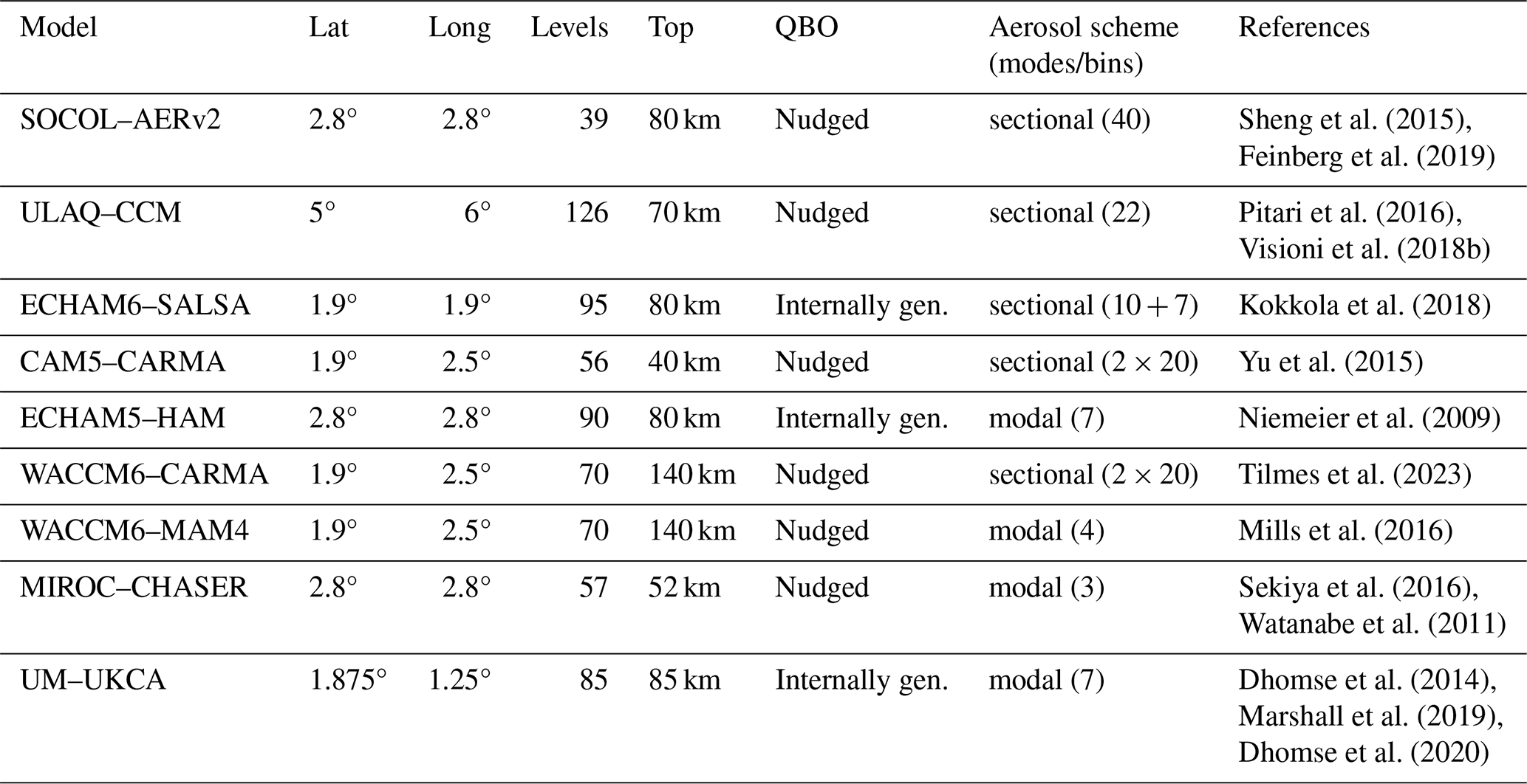
^* https://isamip.eu/home (last access: 23 April 2024)

2.2.2 ULAQ–CCM

The global-scale chemistry–climate model ULAQ–CCM (University of L'Aquila Chemistry Climate Model) has a resolution of 5° × 6° (T21) and uses 126 log-pressure levels, reaching from the Earth's surface to 0.04 hPa. It treats sulfate, organic and black carbon, dust, sea salt, nitrate, and polar stratospheric cloud (PSC) aerosols (Pitari et al., 2002). Each type of aerosol is treated separately in terms of surface fluxes, transport, and removal from the atmosphere. The wet and dry deposition schemes are based on Müller and Brasseur (1995). Included in the chemistry module are species from the O_x, NO_y, NO_x, CHO_x, HO_x, Cl_y, Br_y, and SO_x families. This includes six sulfur species: OCS, CS₂, DMS, H₂S, H₂SO₄, and SO₂, as well as the long-lived species N₂O, CH₄, CO, hydrocarbons, CFCs, hydrochlorofluorocarbons, and halons. (Pitari et al., 2016; Visioni et al., 2018a). For ULAQ, only 10 years of the simulation were conducted.

2.2.3 WACCM6–CARMA and WACCM6–MAM4

In this study, we include simulations with the Community Earth System Model version 2 (Danabasoglu et al., 2020) in its high-top configuration, named the Whole Atmosphere Community Climate Model version 6 (WACCM6). We use the middle atmosphere (MA) chemistry mechanism (Gettelman et al., 2019). Hereafter, we call this model setup WACCM6–MA. In our setup, WACCM6–MA has 70 vertical levels reaching up to 140 km above the surface. We set the horizontal resolution of 1.9° × 2.5°. This model includes a comprehensive chemistry scheme in the stratosphere, mesosphere, and lower thermosphere, while only representing limited chemistry in the troposphere (Gettelman et al., 2019). The model accounts for sulfur chemistry of important precursor emissions for both the troposphere and stratosphere, including four sulfur species, namely OCS, DMS, SO₂, and H₂SO₄ (Mills et al., 2016).

WACCM6 is coupled to two different aerosol microphysical modules. The Modal Aerosol Model (MAM4) (Liu et al., 2012, 2016), which includes updated prognostic stratospheric sulfate aerosols (Mills et al., 2016), is the default aerosol scheme used in CAM-chem and WACCM6 of CESM2. Four modes are described by MAM4 microphysics: Aitken, accumulation, and coarse modes, as well as a primary carbon mode (Liu et al., 2016). The geometric standard deviation of MAM4 for the Aitken and accumulation mode is 1.6, while for the coarse mode, it is 1.2 (Liu et al., 2016; Mills et al., 2016).

The second aerosol microphysical model coupled to WACCM6 is the Community Aerosol and Radiation Model for Atmospheres (CARMA) version 4.0, which enables size-resolved or sectional cloud droplets and aerosol particles (Toon et al., 1988). The CARMA aerosol model includes prognostic aerosols for both the troposphere and the stratosphere, as discussed in Yu et al. (2015), and additional changes are highlighted in Tilmes et al. (2023). Apart from pure sulfate aerosol, WACCM6–CARMA is one of two models participating in this study which includes an internally mixed group of aerosol. It involves sulfate, primary and secondary organics, black carbon, dust, and sea salt. The model divides each group into 20 discrete mass bins, as defined by Yu et al. (2015). The mixed aerosol group specifies bins with radii between 0.05 and 8.7 µm, whereas radii of the pure sulfate group range from 0.2 nm to 1.3 µm. The aerosol composition is based on Tabazadeh et al. (1997).

2.2.4 ECHAM6–SALSA

The aerosol–climate model ECHAM6–SALSA (ECHAM6.3–HAM2.3–MOZ1.0–SALSA2.0 is comprised of the ECHAM6.3 general circulation model (Stevens et al., 2013) and the HAM aerosol module (Tegen et al., 2019). The last component is the aerosol microphysics module SALSA2.0 (Kokkola et al., 2018). The model was set up with a T63 resolution, corresponding to a 1.9×1.9 horizontal grid. Furthermore, it uses 95 vertical levels with a top at 0.01 hPa. The microphysical scheme SALSA uses 10 fixed size bins, ranging from 3 nm to 10 µm, while the seven largest bins additionally treat soluble and insoluble aerosol (Kokkola et al., 2018). In this study, we use the parameterized sulfuric acid–water binary homogeneous nucleation parameterization (Vehkamäki et al., 2002) for nucleation. The analytical predictor of condensation (APC) scheme is applied to calculate condensation (Jacobson, 1997), while coagulation is treated according to Lehtinen et al. (2004). Apart from sulfate, SALSA also includes organic aerosol, sea salt, black carbon, and mineral dust. The deposition and sedimentation in SALSA are presented by Bergman et al. (2012). ECHAM6–SALSA uses a simplified chemistry scheme from HAM (Feichter et al., 1996; Zhang et al., 2012) and includes the oxidation of DMS and SO₂ via a range of oxidizing agents (OH, H₂O₂, NO₂, and O₃) prescribed by a monthly mean climatology. ECHAM6–SALSA includes three of the main sulfur gases (DMS, SO₂, and H₂SO₄), whereas OCS is not included.

2.2.5 ECHAM5–HAM

ECHAM5–HAM uses the high-top version of ECHAM5 (Giorgetta et al., 2006) and is coupled to HAM, an aerosol microphysical model (Stier et al., 2005). The horizontal grid has a 2.8° × 2.8° resolution, whereas vertically, there are 90 layers up to 0.01 hPa, corresponding to 80 km. Microphysics in HAM treats the oxidation of sulfur, including sulfate aerosol formation. This encompasses nucleation, accumulation, condensation/evaporation, and coagulation. To improve the stratospheric aerosol representation, modifications were made to the microphysical core M7 (Vignati et al., 2004) of HAM (Niemeier et al., 2009), especially for high sulfur loads after volcanic eruptions. HAM uses a modal size distribution comprised of four modes. The simulations for this paper used the nucleation, Aitken, and accumulation mode with a mode width of 1.59 and a coarse mode with a mode width of 2. Another addition was made to HAM in the form of a simple stratospheric sulfur chemistry scheme (Timmreck, 2001; Hommel et al., 2015). The sulfur chemistry in ECHAM5–HAM tracks four sulfur gases, namely OCS, DMS, SO₂, and H₂SO₄. As the chemistry scheme is not fully interactive, monthly fields for OH, NO₂, and O₃, as well as photolysis rates of OCS, H₂SO₄, SO₂, and O₃ are prescribed on a monthly mean basis. A general description of the performance of HAM is described in Stier et al. (2005), Zhang et al. (2012), and Niemeier and Timmreck (2015).

2.2.6 CAM5–CARMA

CAM5–CARMA is a low-top version of the Community Earth System Model (CESM1), coupled to the aerosol microphysical model CARMA, which is described in Sect. 2.2.3. It has a horizontal resolution of 1.9° × 2.5° and runs on hybrid 56 vertical levels (Yu et al., 2015). The model includes full stratospheric and tropospheric chemistry, using the chemistry module MOZART-4 (Emmons et al., 2010). CARMA tracks organic carbon, black carbon, dust, and sea salt, as well as an internally mixed type (Yu et al., 2015). Secondary organic aerosol is included and based on Pye et al. (2010). CARMA provides a sectional aerosol scheme, tracking 20 particle size bins for aerosol and another 20 for mixed aerosol. DMS emissions are based on Kloster et al. (2006). The chemistry scheme in CAM5–CARMA includes 230 chemical reactions. Sulfur chemistry is based on English et al. (2011) and includes 22 gas-phase and 5 heterogeneous reactions, summarized in Yu et al. (2015). Three sulfur species are tracked in CAM5–CARMA, additionally to sulfate aerosol, namely OCS, SO₂, and H₂SO₄. For this simulation, CAM5–CARMA was nudged to the MERRA-2 reanalysis. Instead of the 20-year time slice simulation, we use 20 ensemble members for the year 2000.

2.2.7 MIROC–CHASER

The global chemistry–climate model MIROC–CHASER (Sudo et al., 2002; Watanabe et al., 2011) consists of the Model for Interdisciplinary Research on Climate (MIROC) and the atmospheric chemistry model CHASER (Sudo et al., 2002; Sudo and Akimoto, 2007) and the Spectral Radiation–Transport Model for Aerosol Species (SPRINTARS) (Watanabe et al., 2011). For this study, the model is set up with a 2.8° × 2.8° horizontal resolution and 57 vertical levels up to 52 km. The aerosol module SPRINTARS tracks sulfate aerosol with three modes (nucleation, Aitken, and accumulation) and uses the bulk approach for black carbon and organic matter, dust, and sea salt (Sekiya et al., 2016). DMS emissions in MIROC–CHASER are a function of downwelling short-wave radiation. Nucleation is based on Vehkamäki et al. (2002), while coagulation follows the same scheme as ECHAM5–HAM (Stier et al., 2005). The chemical scheme in CHASER includes 93 species, as well as 263 reactions. Sulfur chemistry is included in the form of 12 reactions, as well as 4 of the main sulfur species (SO₂, SO₄, DMS, OCS) (Sekiya et al., 2016).

2.2.8 GA4-UM–UKCA

The first GA4-UM–UKCA (hereafter UM–UKCA) simulation submitted for the ISA–MIP BG_QBO (here called REF) experiment (Timmreck et al., 2018) uses the interactive stratospheric aerosol configuration of the UM–UKCA model (Bellouin et al., 2013; Dhomse et al., 2014). The model runs with a horizontal resolution of 1.875° × 1.25° and on 85 levels, with a model top at approximately 85 km. Specifically, this first UM–UKCA submission to BG applies the identical version 3 (v3) stratosphere–troposphere UKCA codebase also run for the ISA–MIP HErSEA–Pinatubo experiment (Dhomse et al., 2020); as further analyzed by Quaglia et al. (2023), each of the ISA–MIP UM–UKCA runs within the GA4 configuration of the UM general circulation model (Walters et al., 2014).

This version 3 of stratosphere–troposphere UM–UKCA comprises version 8.2 of the GLOMAP-mode aerosol microphysics module (see Dhomse et al., 2020) implemented within the RJ4.0 configuration of the UK Chemistry and Aerosol sub-model, as released to the UK academic community within GA4 (Abraham et al., 2012). The chemical scheme accounts for OCS, SO₂, DMS, H₂SO₄, SO₃, and sulfate aerosol (Dhomse et al., 2014). For the REF experiment, the simulations are within the year 2000 time slice atmosphere-only simulations, with boundary conditions and tropospheric chemistry and aerosol emissions identical to that described by Abraham (2014) and with the aerosol–radiation and aerosol–cloud interaction radiative effects and UM–UKCA simulated tropospheric and stratospheric ozone layers fully interactive with the radiative transfer module within GA4.

The 20-year simulation analyzed is the last 5 years from the UM–UKCA v3 simulation shown in Brooke et al. (2017), with an extension for a further 15 years for the REF experiment. As explained in Dhomse et al. (2020), v3 UM–UKCA includes heterogeneously nucleated sulfuric acid aerosol particles with the 7.9 t d⁻¹ meteoric smoke particle (MSP) climatology (v3 low MSP). As configured for the analysis in Brooke et al. (2017), the simulation has the modal desert dust emissions switched off, with desert dust radiative effects from the UM sectional interactive dust scheme (Woodward, 2001, 2011) rather than from GLOMAP-mode.

The TS2000 atmosphere-only RJ4.0 UM–UKCA model used here is identical to that also applied for the 2000 volcanic forcing perturbed-parameter ensemble (Marshall et al., 2019, 2021) and equivalent also to the pre-industrial setting GA4 UM–UKCA v3 simulations for the Volcanic Forcings Model Intercomparison Project (VolMIP) interactive Tambora experiment (Marshall et al., 2018; Clyne et al., 2021).

2.3 Observational and reanalysis data

We use several satellite-derived datasets for the stratospheric aerosol layer (NASA/LARC/SD/ASDC, 2012; Damadeo et al., 2013; Revell et al., 2017), stratospheric SO₂ (Höpfner et al., 2013, 2015), stratospheric OCS (Glatthor et al., 2017), and in situ measurements from high-altitude balloon soundings (Deshler et al., 2019). An overview of these datasets is provided in Table 2.

For each of these datasets, we use the period 1999–2004 (unless otherwise specified) that is relatively unaffected by volcanic eruptions. Comparing transient observations with time slice simulations comes with certain caveats, including the influence of the QBO. The influence of the QBO is not limited to the tropical stratosphere but also affects export from the tropics to mid-latitudes and modulates the strength of the winter polar vortex (Baldwin et al., 2001). Therefore, we do not try to validate models against observational data. Rather, we attempt to qualitatively assess the differences and refer the reader to previous papers in which quantitative model validations have been conducted.

Eyring et al. (2016)Kovilakam et al. (2023)Kovilakam et al. (2020)Höpfner et al. (2013, 2015)Glatthor et al. (2017)Damadeo et al. (2013)NASA/LARC/SD/ASDC (2012)Dee et al. (2011)Deshler et al. (2019)

Table 2 Observational and reanalysis datasets used in this study and the original resolution of each dataset.

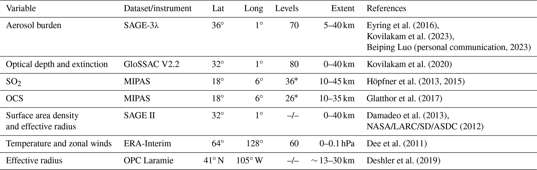
^* The numbers of levels for MIPAS do not reflect the vertical resolution. These are provided in the dataset and the related publications
(Höpfner et al., 2013, 2015; Glatthor et al., 2017).

We use an aerosol dataset derived using the 3-λ mechanism, as described by Revell et al. (2017), which is based on the Global Space-based Stratospheric Aerosol Climatology version 2.2 (GloSSACv2.2) dataset (see below). These data are derived from extinction measurements at three wavelengths by the Stratospheric Aerosol and Gas Experiment II (SAGE II; Thomason et al., 2018). The dataset, hereafter called SAGE-3λ, includes the zonal mean distribution of aqueous H₂SO₄ concentrations as monthly mean values from 1979–2021 at 36 latitudes, where the data beyond 80° N and S have been extrapolated. ¹ SAGE-3λ provides data at altitudes every 500 m between 5 km and 40 km. We apply this dataset above the lapse rate tropopause derived from ERA-Interim (ERA-I) temperature data (Dee et al., 2011).

We evaluate the model-derived extinctions at ∼ 525 nm (the wavelength corresponding to SAGE II data with the smallest uncertainty) and compare them with the GloSSACv2.2 data, although optical properties are not the main focus of this analysis. The GloSSACv2.2 dataset includes the solar occultation SAGE II measurements at four wavelengths out of the seven SAGE II wavelengths available (Kovilakam et al., 2020; NASA/LARC/SD/ASDC, 2022). The dataset is composed of monthly zonal mean values at 32 latitudes, ranging from 80° N to 80° S and vertical levels from 0.5 to 40 km at 500 m intervals.

A dedicated level-3 dataset for SO₂, derived from the Michelson Interferometer for Passive Atmospheric Sounding (MIPAS), is used in the present study. To achieve global distributions of SO₂ with a vertical coverage from 10 to 45 km we have combined two datasets: (1) the gridded dataset used in Schallock et al. (2023), based on the MIPAS single retrievals (Höpfner et al., 2015) from 10 to 23 km altitude and 5 d binning, and (2) the MIPAS monthly mean retrievals, with a vertical coverage of 15–45 km (Höpfner et al., 2013). To minimize the volcanic influence, several months in the dataset that appeared to be affected by eruptions were excluded from the analysis, as described by Höpfner et al. (2015). As this leaves significant gaps in the dataset, we use an average over the whole period from 2002 to 2012 for our analysis. Furthermore, we use the temperature distribution from ERA-I to derive the lapse rate tropopause and calculate stratospheric burdens.

For OCS, we utilized a gridded dataset based on the MIPAS retrievals by Glatthor et al. (2017) with a three-dimensional sampling of 10° latitude, 60° longitude, and 1 km altitude with a vertical coverage of 10 to 35 km and a temporal averaging of 5 d. The temporal coverage of this dataset from July 2002 to April 2012 does not include the first 3.5 years of our chosen time period. However, since OCS does not significantly depend on volcanic emissions and trends in background OCS are small, these influences are disregarded here (Kremser et al., 2016). To calculate stratospheric burdens, the ERA-I-derived tropopause was applied.

We also use the effective radius and aerosol surface area density dataset derived from SAGE II with the SAGE version 7.0 algorithm (Damadeo et al., 2013; NASA/LARC/SD/ASDC, 2012). Aerosol was assumed to be composed of aqueous sulfuric acid solution at 75 wt % H₂SO₄.

We also compare the simulated size distributions to balloon measurements from Laramie, Wyoming, at 41° N and 104° W (Deshler and Kalnajs, 2022). The data have been collected using optical particle counters (OPCs), which measure the particle concentration in 12 size bins from 0.15–2 µm (Deshler et al., 2019).

3 Results and discussion

3.1 The global atmospheric sulfur budget

In Fig. 1, we present the global atmospheric sulfur budget represented by burdens and fluxes of major sulfur species, based on the input by the nine global atmospheric aerosol models involved in this study (see Table 1). The major sulfur (S) species are specified in gigagrams of sulfur of each sulfur species (Gg (S)) for the burdens and gigagrams of sulfur of each sulfur species per year (Gg (S) yr⁻¹) for fluxes. For the four models CAM5–CARMA, WACCM6–CARMA, WACCM6–MAM4, and UM–UKCA, stratospheric burdens are calculated from monthly mean volume or mass mixing ratios integrated from the model tropopause upward, as these burdens were not directly provided by some of the modeling groups. Mean emission and deposition fluxes are calculated by averaging the corresponding output from those models that provided them.

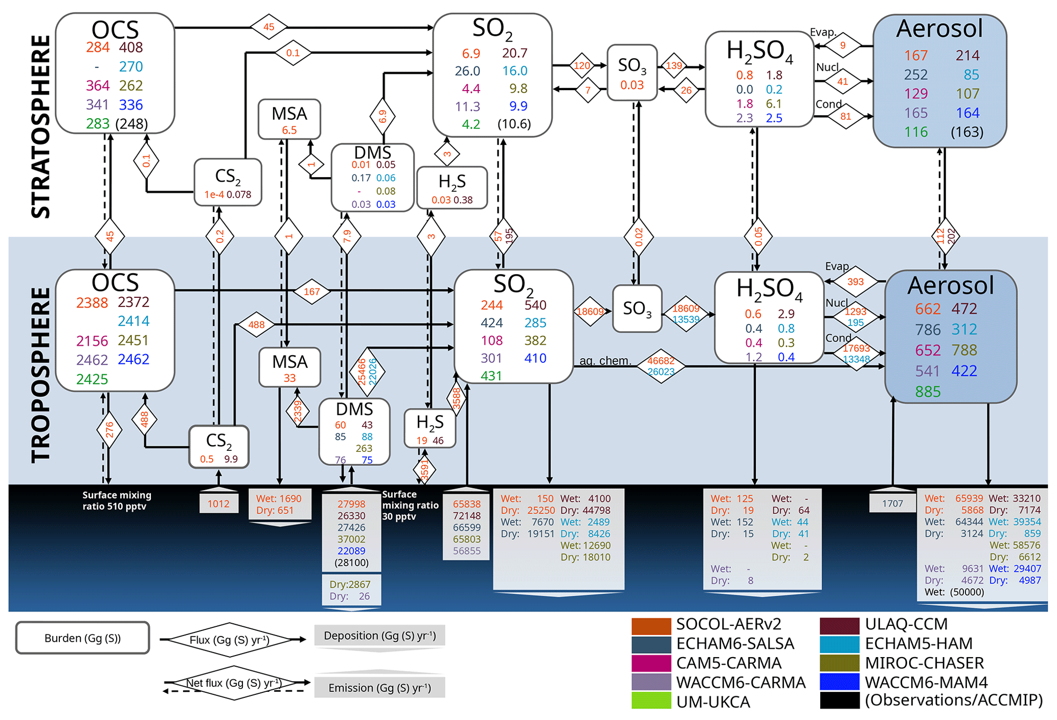
Figure 1 The atmospheric sulfur cycle with burdens (in Gg (S)) and fluxes (Gg (S) yr⁻¹) for S gases and sulfate aerosols (displayed in analogy to Feinberg et al., 2019, and Sheng et al., 2015). The term “aerosol” refers only to sulfate aerosol. The figure includes all burdens as provided by the models involved. For CAM5–CARMA, WACCM6–CARMA, WACCM6–MAM4, and UM–UKCA, stratospheric burdens are calculated from the monthly mean volume or mass mixing ratios integrated from the model tropopause upward because these burden values were not provided. Burdens and fluxes are averaged over the entire period. We use SAGE-3λ for aerosol and MIPAS for SO₂ and DMS emissions from Lana et al. (2011), which are all observation-derived. Additionally, we show the aerosol wet depositions from a multi-model mean from the Atmospheric Chemistry and Climate Model Intercomparison Project (ACCMIP) (Lamarque et al., 2013), as previously used in Feinberg et al. (2019). These observation-derived data and the ACCMIP values are in parentheses. Most fluxes are given as one-way fluxes, while cross-tropopause transport values, as well as OCS and H₂S emissions, are provided as net fluxes. Fluxes are only available for one or two models at a time (SOCOL–AERv2 and ULAQ–CCM or SOCOL–AERv2 and ECHAM5–HAM). Emissions of OCS and H₂S were prescribed as mixing ratios in the surface layer in some models. In that case, emission and deposition net fluxes for both species are derived by balancing the sum of the other fluxes of all species.

Table 3 The multi-model mean, standard deviation, and coefficient of variation in all major species in the troposphere, the stratosphere, and their emissions and depositions. The total tropospheric burden, total stratospheric burden, total emission, and total deposition include the values from all species and the fraction of each compound of the total mass of sulfur in each category.

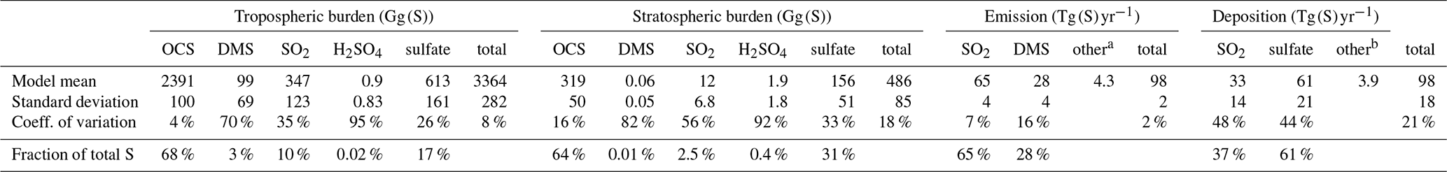
^a Available only from SOCOL–AERv2 by summing up the chemical fluxes from H₂S, CS₂, and OCS to SO₂. ^b DMS, H₂SO₄, and MSA, with DMS being based on MIROC–CHASER and WACCM6–CARMA and MSA being based only on SOCOL–AERv2.

Observational data, as well as one ACCMIP estimate (in parentheses), are from the SAGE-3λ and MIPAS datasets described in Sect. 2.3 for stratospheric sulfate aerosol, SO₂, OCS, and DMS emissions, respectively, and the aerosol wet deposition rates. Figure 1 is constructed in analogy to the figures of the sulfur cycle shown by Feinberg et al. (2019) and Sheng et al. (2015). Subsequently, we refer to sulfate aerosol often simply as aerosol. Additionally, we present the multi-model mean, standard deviation, and coefficient of variation in Table 3. The coefficients of variation are calculated as the standard deviation divided by the model mean. Mean burdens are calculated by averaging the output of all nine models (except OCS, which is an average over eight models without ECHAM6–SALSA, which does not treat OCS).

3.1.1 Precursor gas emissions

Sulfur emissions are dominated by SO₂ with 65452 ± 4483 Gg (S) yr⁻¹ (model mean plus/minus standard deviation; see Table 3). These emissions are largely of anthropogenic origin, as shown in Fig. A1, where we compare the natural-only versus all emissions in the NAT and REF simulations (from the MACCity inventory). Under anthropogenically perturbed conditions, emissions dominate in the Northern Hemisphere (NH) and are widely present over the ocean as well, in comparison to only natural emissions. In Fig. 1, ULAQ–CCM has slightly higher and WACCM6–CARMA lower SO₂ emissions than the other models. The second-strongest emissions are those of DMS, which show a large model spread, with a mean and standard deviation of 28169 ± 4453 Gg (S) yr⁻¹. DMS emissions vary the most (with a coefficient of variation of 16 %; see Table 3). Models typically calculate DMS emissions online as a function of wind speed and prescribed concentration of DMS in seawater. Large variations in DMS emissions have also been shown in a previous model comparison by Textor et al. (2006). As an important precursor for tropospheric SO₂ (see fluxes provided by ECHAM5–HAM and SOCOL–AERv2 in Fig. 1), this influences tropospheric SO₂ burdens. Figure 1 also shows the model results for OCS and H₂S for the models in which surface mixing ratios are specified instead of emissions. Their contribution to other sulfur-containing species can be tracked via the chemical fluxes provided by the SOCOL–AERv2 model. Their net surface flux is also shown for SOCOL–AERv2, calculated by balancing all other fluxes. Furthermore, ECHAM6–SALSA, WACCM6–CARMA, and WACCM6–MAM4 also include primary sulfate aerosol emissions. For example, in ECHAM6–SALSA, 2.5 % of all anthropogenic, wildfire, and volcanic sulfur emissions are emitted as sulfate aerosol particles. Finally, CS₂ is included by prescribing emissions; CS₂ is the dominant precursor to the important OCS (but not all models include this process in their chemistry scheme, since OCS is defined by a fixed mixing ratio). Sheng et al. (2015) performed sensitivity experiments with the SOCOL–AERv1 model by isolating the contribution of specific sulfur emissions to the stratospheric aerosol layer. They found that OCS contributes around half to the stratospheric burden, SO₂ one-third, and the rest is mostly from DMS. However, their estimate for the total stratospheric aerosol burden was 109 Gg (S), which is lower than the value obtained with the new model version (167 Gg (S) in Fig. 1).

3.1.2 Global tropospheric burdens

Although the implementation details of the sulfur cycle vary widely among the different models, most of them include the following three dominant species: OCS, SO₂, and sulfate aerosol. Calculating the model means of all species in Fig. 1, OCS accounts for about 68 % of the total mass of sulfur in the troposphere and varies very little among models with a coefficient of variation of 4 % (see Table 3). This is not surprising because this species is prescribed at the surface and has few chemical sinks in the troposphere, while sinks such as plant uptake are not explicitly modeled. Sulfate and SO₂ represent 17 % and 10 % of the total tropospheric sulfur mass, respectively, though inter-model differences are much larger than for OCS. SO₂ burdens range from 108 Gg (S) in CAM5–CARMA to 5 times that amount in ULAQ–CCM. Tropospheric aerosol also varies between the lowest values in ECHAM5–HAM at 312 Gg(S) and the highest in UM–UKCA (885 Gg (S)). However, in all models, these species are dominant and leave about 5 % tropospheric sulfur in the form of DMS, MSA, H₂S, CS₂, gas-phase H₂SO₄, and SO₃. The latter species are present only in small amounts as a result of their respective short lifetimes (1 to a few days in the atmosphere) (SPARC, 2006; Chen et al., 2018) or low vapor pressure in the case of H₂SO₄. In contrast, SO₂ remains in the atmosphere for about 10 d and OCS for 2 years (Khalil and Rasmussen, 1984). However, the less abundant species fulfill an important role as precursor gases for sulfate particles. In addition, there are intermediate products of photolysis and oxidation (SPARC, 2006, and references therein), but they are even more short-lived and so are not shown here.

3.1.3 Global stratospheric burdens

The stratosphere shows a similar distribution of relative abundances as in the troposphere, with OCS accounting for about 64 % total stratospheric sulfur, while aerosol is 31 % and SO₂ is 2.5 % (see Table 3). Based on its abundance and its lifetime, OCS was identified as the main precursor for background sulfate aerosol by Crutzen (1976) (see also Sheng et al., 2015). OCS is primarily a product of photolysis and subsequent oxidation of other precursor gases, such as CS₂ (SPARC, 2006). It is characterized by a long tropospheric lifetime and is removed from the atmosphere mainly via plant uptake in the troposphere and photo-oxidation to H₂SO₄ in the stratosphere (Barkley et al., 2008). The variation between the models is 16 %, i.e., somewhat larger in the stratosphere than in the troposphere, with outliers at as much as 28 % above the model mean (ULAQ–CCM). The lifetime of OCS is still very long in the stratosphere (years). Therefore, the importance of dynamical (meridional and cross-tropopause transport) and chemical (photolysis) sinks increases. This increases the multi-model spread, given that individual models necessarily have some biases in their representation of dynamical processes. This is discussed further in the context of the spatial distribution in Sect. 3.3.2. Models tend to overestimate the stratospheric OCS burden when compared to MIPAS. The MIPAS dataset only extends to 35 km (Table 2). However, not much OCS is present above this altitude due to photolysis (see Fig. 6).

SO₂ represents an important step in the atmospheric sulfur oxidation chain, as all precursor gases are first oxidized to SO₂, from there to SO₃, and then to gaseous H₂SO₄, which co-condenses with H₂O to form aerosol particles. The stratospheric SO₂ burden reveals the largest scatter among the three major species (coefficients of variation in Table 3 of ± 56 %), with a factor of 5 difference between the models with the smallest and largest burdens. Although the model spread is large, MIPAS is close to the overall mean of stratospheric SO₂ burden. We can group the models in Fig. 1 into three groups with respect to SO₂. SOCOL–AERv2, CAM5–CARMA, and UM–UKCA have the lowest burdens, while WACCM6–CARMA, WACCM6–MAM4, and MIROC–CHASER are in the middle range (and closest to MIPAS), and ULAQ–CCM, ECHAM6–SALSA, and ECHAM5–HAM have significantly higher burdens of SO₂ than the other models. The spatial distribution and plausible reasons for these differences are discussed in Sect. 3.3. Sources of SO₂ in the stratosphere include photo-oxidation of OCS and, just as important, the transport of tropospheric SO₂ across the tropopause. Uncertainties remain regarding the transport of SO₂ to the stratosphere (Kremser et al., 2016), which, besides the complexity of the upper troposphere and lower stratosphere (UTLS) transport processes themselves, could also be very sensitive to how the models treat the aqueous oxidation processes in the upper troposphere (Feinberg et al., 2019). Tropospheric aqueous and gas-phase SO₂ oxidation fluxes are presented in Fig. 1 for SOCOL–AERv2 and ECHAM5–HAM; however, ECHAM5–HAM shows lower values for both pathways. In the lower stratosphere, SO₂ lifetime for oxidation by OH is 3–4 weeks, making it the source of H₂SO₄ and subsequently the Junge aerosol. From these considerations, it appears that most of the models underestimate the turnover in the chemical reaction of SO₂ + OH.

The stratospheric aerosol burden is about 156 ± 51 Gg sulfur in the multi-model mean (with standard deviation; see Table 3). This value differs only slightly from the value derived from the SAGE-3λ observational dataset described by Revell et al. (2017, and personal communication with Beiping Luo, 2023). The scatter between the models is rather small; however, it still has a coefficient of variation of 33 % with a factor of 3 difference between model outliers. The reduced scatter for aerosol compared to SO₂ is due to the much longer residence time of aerosol in the stratosphere, as well as the contribution of tropospheric aerosol. A slightly shorter or longer chemical lifetime of SO₂ does therefore not affect the SO₂ burden and the aerosol burden equally. The scatter of aerosol also does not match the scatter of OCS in the stratosphere because OCS accounts for only about half of the source of stratospheric aerosol, with the other half being the cross-tropopause fluxes of SO₂ and aerosol itself (Sheng et al., 2015). In our analysis, unfortunately, only the net cross-tropopause fluxes are available and also only from a few models, which limits the analysis in the attribution of stratospheric biases. In addition, the model differences in stratospheric aerosol loading can also be caused by differences in sedimentation fluxes among models, which in turn depends on aerosol size distribution. Sheng et al. (2015) and Delaygue et al. (2015) estimated that gravitational sedimentation reduces the background stratospheric aerosol burden by about half. In comparison, ECHAM5–HAM exhibits an unusually low aerosol burden. This is likely the result of anomalous concentrations of OH and, thus, slower SO₂ oxidation in the stratosphere, as discussed in Sect. 3.2. Other factors may also contribute, such as differences in the vertical residual velocity in the tropics, which was identified by Niemeier et al. (2020) as a cause of major differences in the aerosol burdens between ECHAM5–HAM and WACCM6. The highest aerosol values are reported by ECHAM6–SALSA. Laakso et al. (2022) discussed how excessive new particle formation may contribute to such an effect. However, it is unclear if this nucleation bias only applies to scenarios with a large disturbance from volcanic eruptions or stratospheric aerosol injections. Conversely, this has not been observed before in ECHAM6–SALSA (see, e.g., Kokkola et al., 2018), with the main difference being the vertical resolution of the model.

Short-lived species, such as DMS and gaseous H₂SO₄ with lifetimes shorter than 1 d, exhibit large scatter between models (with models differing by more than 1 order of magnitude), but the uncertainties in these burdens do not significantly affect the ones of longer-lived species. Rather, one would need to investigate the reaction rates to determine the processes leading to differences in the burdens of the major species.

Figure 2 presents the total integrated sulfur burdens. The total emission and deposition rates in ECHAM6–SALSA do not include OCS but are in the same range as most other models, while the total S burden is lower by about the amount of OCS in the other models. However, ECHAM6–SALSA has the highest SO₂ burden out of all models, making more of it available for oxidation and the formation of aerosol. Deposition is again in the same range as other models, meaning that aerosol may accumulate more.

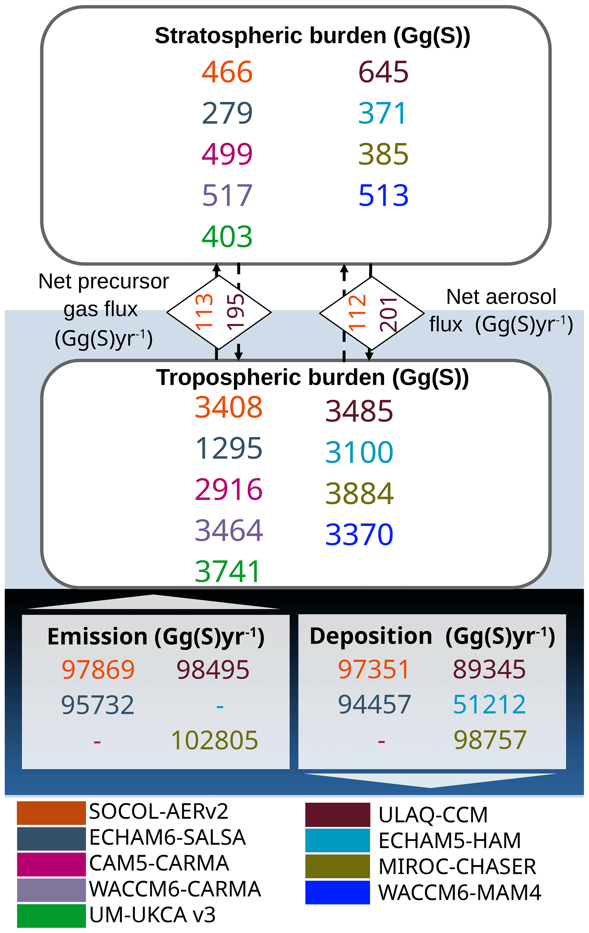
Figure 2 The total sulfur balance for each model. All sulfur species are summed up for each model and depicted here (in Gg (S)). Cross-tropopause fluxes (in Gg (S) yr⁻¹) are net fluxes of aerosol precursor gases (net upward) plus the net aerosol flux (net downward), which were only provided by SOCOL–AERv2 and ULAQ–CCM. The burden for ECHAM6–SALSA is lower, as the model does not include OCS. Therefore, this model is excluded from the calculation of the model spread for the total sulfur burden.

3.1.4 Wet and dry deposition rates

Deposition rates are mainly available for sulfate aerosol, which is dominated by wet deposition, and for SO₂, which is dominated by dry deposition, consistent among all models. Some species, such as CS₂ or DMS, are often considered to be entirely chemically processed and therefore not deposited. While wet and dry deposition rates vary considerably (see for SO₂ or aerosol in Fig. 1), the total deposition of sulfur remains similar among models, as seen in Fig. 2. This is not surprising because the total sulfur emission flux is meant to be the same (or at least similar) for all models. All emitted sulfur has to be deposited back to the surface, assuming that models do not have large errors in mass conservation. ECHAM5–HAM is a strong outlier in terms of total sulfur deposition, with the reason being currently unclear, given that other fluxes available for this model (DMS conversion to SO₂, SO₂ emission, and oxidation fluxes) do not differ much from other models. Textor et al. (2006) discussed the partitioning of sulfur deposition in a global model intercomparison for tropospheric aerosol. They found that, in some models, sulfur is already deposited in the form of precursor gases, therefore resulting in a lower burden and less deposition in the aerosol phase. Here, we see that ULAQ–CCM, ECHAM5–HAM, and WACCM6–MAM, which have lower tropospheric aerosol burdens, also exhibit lower total aerosol deposition rates compared to the other models. However, when adding all reported deposition fluxes together, ECHAM5–HAM has the highest percentage (79 % deposited sulfur) deposited as aerosol, while ULAQ–CCM has the lowest at 45 %. Therefore, in ECHAM5–HAM another process must be influencing the deposition rates. Most aerosol is wet deposited, which is consistent with Textor et al. (2006). The total aerosol deposition shown in Fig. A2a–f indicates that it is not just the amount but the spatial distribution of the aerosol deposition that varies considerably among models, though it still mostly resembles the global distribution of precipitation (e.g., Tapiador et al., 2017). Regional differences are influenced by both the aerosol formation processes and the biases in the models' precipitation patterns and the details of deposition schemes (Textor et al., 2006; Marshall et al., 2018). In all models, the anthropogenic aerosol (Fig. A2g–i) deposits mostly in the regions where the anthropogenic emission of SO₂ takes place (Fig. A1). This confirms the short tropospheric lifetime of the aerosol, limiting its long-distance transport. In ECHAM5–HAM, 98 % of the aerosol deposition is wet deposition, followed by 95 % in ECHAM6–SALSA, 92 % in SOCOL–AERv2, 90 % MIROC–CHASER, 86 % in WACCM6–MAM4, and finally ULAQ–CCM with the lowest percentage at 82 % wet deposition.

For SO₂, the dry deposition dominates but varies strongly between models, with 99 % for SOCOL–AERv2, 92 % for ULAQ–CCM, 77 % for ECHAM5–HAM, 71 % for ECHAM6–SALSA, and only 59 % in MIROC–CHASER.

3.1.5 Total atmospheric sulfur burden

We present the total sulfur burden in the stratosphere and troposphere in Fig. 2. Although the models have chemistry schemes of various complexities, which affects the partitioning between the sulfur species, the total sulfur burden is similar across models, at 3861 ± 294 Gg (S), for the models including the main three sulfur species OCS, SO₂, and sulfate aerosol (therefore excluding ECHAM6–SALSA). This corresponds to 485 ± 85 Gg (S) in the stratosphere (12.6 % of all atmospheric sulfur) and 3375 ± 284 Gg (S) in the troposphere. The relative difference among models is higher in the stratosphere, as discussed in Sect. 3.3. Figure 2 also presents estimates from SOCOL–AERv2 and ULAQ–CCM of the net cross-tropopause fluxes of aerosol and aerosol precursors. The two models agree that the sign of the net fluxes is directed upward for precursors and downward for aerosol but disagree on their magnitudes. These fluxes are not fully balanced, although they are expected to be somewhat in equilibrium. The reason for ULAQ–CCM is that only the SO₂ flux is available, and the contribution of other species (mainly OCS and DMS, as seen from SOCOL–AERv2 data in Fig. 1) is missing. SOCOL–AERv2 takes all the species into account; therefore, the imbalance could be a result of deficient mass conservation in its transport scheme, especially where the tracer gradients are steep (Stenke et al., 2013). As for emissions and deposition fluxes, the values provided in the figure are quite scattered because not all variables calculated by models were present in the output provided in the model database and could therefore not be included in our budget calculations. This also explains the inconsistency between the total deposition and the emission fluxes for individual models. All the required output was only provided for SOCOL–AERv2. As a result, the full emission and deposition fluxes for this model are calculated by including the chemical fluxes of minor precursors to SO₂, resulting in a good agreement between the two. In all other models, these data were not provided in the output, therefore statements about their mass conservation cannot be made. In terms of the model mean values presented in Table 3, individual model nuances are averaged out, resulting in a flux of 98 Tg (S) for both the total emission and deposition.

3.2 Seasonal cycle of sulfur compounds

Figure 3 shows the seasonal cycle of the most abundant sulfur compounds in the atmosphere, as well as one of the main oxidizing agents of the atmosphere, the hydroxyl radical (OH). Also depicted in (Fig. 3a–e) is the relationship between the stratospheric sulfate burden and the stratospheric aerosol optical depth (SAOD) at ∼ 0.5 µm for each model, season, and latitude. We see for all species, the multi-model spread is the smallest in the tropical region (here at 30° N–30° S), where the burdens are also lower. The relationship between SAOD and the aerosol burden shows little seasonal dependence and very little scatter. In the extratropics, the burdens of sulfur species are higher, suggesting additional transport through the subtropical tropopause and a larger spread among the models in terms of the relation of SAOD and aerosol mass. This suggests a larger divergence in the aerosol size distribution in the extratropics than in the tropics. Additionally, we see a distinct seasonal cycle in all species outside the tropical region and an increased seasonality of the SAOD/aerosol mass relation in many models.

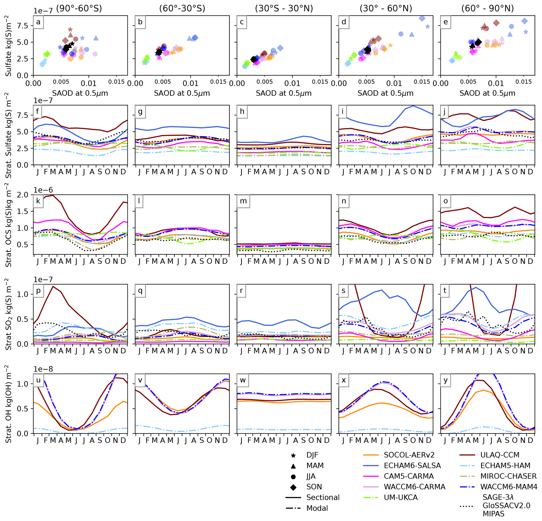
Figure 3 The seasonal cycle of the three most abundant atmospheric sulfur species (sulfate aerosol, SO₂, and OCS), as well as OH (OH was only reported by five models). All data were zonally averaged over the latitude band given in each column title. Additionally, panels (a)–(e) represent the relationship between the SAOD at 0.5μm and the sulfate burden for five latitude bins. Each season is depicted by a character, with a star for winter, a triangle for spring, a circle for summer, and a diamond for autumn. Panels (f)–(j) depict the seasonal cycle of the stratospheric aerosol burden for each of these latitude bins. In panels (k)–(o), we see the stratospheric OCS burden, while panels (p)–(t) show the stratospheric SO₂ burden and panel (u)–(y) the stratospheric OH burden, respectively. Each burden is given (in kg (S) m⁻²), except for OH (given as kg (OH) m⁻²). All data have been averaged over the 20 simulated years for each month. Not shown in the figure are the maximum values of the stratospheric SO₂ burden in ULAQ–CCM and the stratospheric OH burden in both WACCM6 models. ULAQ–CCM SO₂ burdens in the northern mid-latitudes peak in January at 1.9 × 10⁻⁷ kg (S) m⁻² or 5.5 × 10⁻⁷ kg (S) m⁻² in the northern polar region. Maximum OH burdens in WACCM6–CARMA and WACCM6–MAM4 in both the NH (July) and SH (December) amount to 1.3 × 10⁻⁸ kg (OH) m⁻².

In addition to an agreement with Fig. 1 in terms of model aerosol burden levels, we observe that the models with higher burdens (ECHAM6–SALSA, ULAQ–CCM) have a stronger seasonal cycle than those with lower burdens (MIROC–CHASER, ECHAM5–HAM, and UM–UKCA). ECHAM6–SALSA has the highest burdens in the low and mid-latitudes. ULAQ–CCM is similar to ECHAM6–SALSA in the NH polar region and even exceeds the burdens in ECHAM6–SALSA in the Southern Hemisphere (SH). For aerosol, we observe a minimum at high latitudes in the vortex (Fig. 1f) from July to October, followed by an increase which can be attributed to the breakup of the southern polar vortex. In winter, the polar vortex edge represents a barrier to mixing and transport, preventing extra-polar sulfate from entering, similar to what has been observed for ozone and other species (Schoberl and Hartmann, 1991). In SAGE-3λ, this minimum occurs about 1 month earlier than in the models. The same pattern is seen for OCS in (Fig. 1k–o). We conclude that this effect is due to dynamics rather than chemistry. This minimum is discussed in more detail in Sect. 3.3.

In the northern mid-latitudes, most models and SAGE-3λ have minimal aerosol burdens in June, July, and August. In contrast, ECHAM6–SALSA and ULAQ–CCM have increasing burdens during this time, as also seen in high northern latitudes. In the 60°–90° N latitude band, however, the seasonality is not as clear in the models as in the other latitude bands. ULAQ–CCM has two distinct peaks around May/April and again in September/October, while ECHAM6–SALSA and MIROC–CHASER have the highest burdens in this region only in October/November; ECHAM5–HAM and both WACCM6 models, as well as SAGE-3λ, can be grouped together with burdens peaking around May, while in SOCOL–AERv2, a seasonal cycle is not distinguishable. This indicates higher uncertainties in the models in this region, which is directly related to large differences in the northern polar vortex climatology and dynamics between the models (Karpechko et al., 2022), as also shown in Fig. A3 for the models participating here. In Fig. A3a.I–i.I in December–February (DJF), zonal winds are weaker and temperatures higher than ERA-I data in the northernmost latitudes in ULAQ–CCM, UM–UKCA, and to a lesser extent also in ECHAM6–SALSA above ∼40 hPa and ECHAM6-HAM and MIROC–CHASER below ∼40 hPa. These differences are, however, rather small in most models (with the largest outlier with temperature anomalies above 7 K being ULAQ–CCM), especially when comparing to differences in the SH, where seasonal cycles are very similar among models despite stronger biases in the southern polar vortex winds and temperatures, as seen in Fig. A3.

Another feature is the similarity between WACCM6–CARMA and WACCM6–MAM4. Considering that the two WACCM6 models share the same dynamical core and chemistry but are coupled to different aerosol microphysical models, this would indicate that the latter does not influence the resulting burden. There are some temperature differences among the two WACCM6 model configurations in the lower stratosphere; however, the statistical significance of this difference has not been tested. A comparison of the three ECHAM-based models (SOCOL–AERv2, ECHAM6–SALSA, and ECHAM5–HAM) is not as straight-forward, as they have different chemistry schemes and different vertical resolutions since they are based on different ECHAM versions, i.e., ECHAM5 in SOCOL–AERv2 and ECHAM5–HAM versus ECHAM6 in ECHAM6–SALSA. We also discuss, in Sect. 3.3, how an internally mixed type of aerosol (including other components additionally to sulfur) in CARMA causes differences in the troposphere. Furthermore, the effective radius varies, as discussed in Sect. 3.4, with potential impacts on SAOD.

The relationship between the SAOD and stratospheric aerosol burden is illustrated in Fig. 3a–e. (We use the pure sulfate SAOD for SOCOL–AERv2 and ULAQ–CCM, whereas in WACCM6–CARMA, it is the SAOD of both pure and mixed aerosol and in all other models, it is the total SAOD). In general, a higher stratospheric aerosol burden also leads to higher SAOD (Fig. 3a–e). This relationship is less clear in the extratropics. The relationship remains highly linear for SAGE-3λ, which is connected to the assumptions on size distributions in the construction of this dataset. As the relationship between burdens and SAOD is very similar among models in the tropics, the conversion schemes in all models are likely to be very similar. The differences in the extratropics hint at different size distributions, which influence the SAOD but not the total mass. This is discussed briefly in Sect. 3.4. Here, WACCM6–MAM4 tends to have lower SAOD than WACCM6–CARMA, revealing differences between the two aerosol schemes.

The seasonal variability in the OCS burden is very similar to that of sulfate aerosol (Fig. 3k–o). The spread in burdens and irregularity in the seasonal cycles appears slightly smaller for OCS. The highest scatter is found in the northern high latitudes, with CAM5–CARMA now also displaying a second peak, as seen in ULAQ–CCM, around October. In MIPAS, the minimum in the southern polar region is about a month earlier than in all models.

For SO₂ in Fig. 3p–t, we can again group models with low and high burdens, as specified in Sect. 3.1, with ULAQ–CCM, ECHAM6–SALSA, and ECHAM5–HAM in the higher range; the WACCM6 models and MIROC–CHASER in the mid-range; and SOCOL–AERv2, CAM5–CARMA, and UM–UKCA at the lower end. Possible reasons for higher SO₂ burden could be less oxidation or more transport across the tropopause. The stratospheric OH burden is provided in Fig. 3u–y. In ECHAM5–HAM, the OH burden is distinctly lower, supporting the hypothesis that less SO₂ is oxidized and hence less H₂SO₄ is available for aerosol formation. Clyne et al. (2021) have previously shown how the prescribed OH fields in ECHAM5–HAM change the aerosol burden after the 1815 Tambora eruption compared to models with interactive OH chemistry. In ULAQ–CCM, stratospheric OH is very close to the values of other models. Additionally, while ECHAM5–HAM is among the highest burdens in all latitudes, burdens in ULAQ–CCM are only elevated in the polar regions and northern mid-latitudes. Figure A3 shows the temperatures in each model compared to the 1999-2004 ERA-I average. In ULAQ–CCM in Fig. A3b.I–b.IV, the winter polar stratosphere is warmer and has weaker westerlies compared to ERA-I, indicating a weaker polar vortex and hence a weaker barrier to transport from mid-latitudes to the poles. The distribution of sulfate and SO₂ in ULAQ–CCM will be discussed in more detail in Sect. 3.3.

Stratospheric OH is too short-lived to be transported. It is mainly formed by the reaction of H₂O with O(¹D), which is a product of O₃ photolysis (Brasseur and Solomon, 2006). Therefore, less OH is available in the wintertime in the middle and high latitudes. Since OH is the most important oxidizing agent for SO₂, we expect lower OH burdens to correspond to higher burdens of SO₂. We see that for those models where OH was provided, SOCOL–AERv2, ULAQ–CCM, and WACCM6–CARMA have higher stratospheric OH loadings than ECHAM5–HAM, with the latter also having a much less pronounced seasonal cycle. However, these differences do not directly translate to differences in SO₂ burden, as shown by ULAQ–CCM, which has a higher SO₂ burden than the other models. Clyne et al. (2021) discussed the importance of interactive OH during volcanically perturbed conditions, where OH is depleted more rapidly by SO₂ oxidation. In non-interactive chemistry schemes, such as in ECHAM5–HAM and ECHAM6–SALSA, the OH fields may need to be adapted for the conditions, or there could be too much OH available after volcanic eruptions if the background OH level is used but too little during quiet conditions if the volcanically depleted OH is used.

3.3 Spatial and vertical distribution

3.3.1 Sulfate aerosol

Figure 4 shows the distribution of aerosol in all models (Fig. 4a–i) and SAGE-3λ (Fig. 4k). The relative standard deviation (RSD, expressed as a percentage of the multi-model mean) distribution in Fig. 4l indicates the regions where the inter-model differences are the largest. Most of the aerosol mass is concentrated close to the surface, especially in tropical regions, and more pronounced in low northern latitudes. This is likely due to higher SO₂ concentrations in these regions, where anthropogenic emissions originating from East Asia are dominant (Smith et al., 2011; Lee et al., 2011). Figure A4g–l compares the sulfate mass mixing ratios of the NAT experiment with the REF experiment. It shows how anthropogenic emissions increase aerosol concentrations by 30 % and up to more than 80 % locally in the NH troposphere and lower stratosphere. The SH is less influenced by anthropogenic emissions. The same feature is seen in the sulfate deposition in Fig. A2g–l, which increases by more than 80 % over large parts of the NH continents. In SOCOL–AERv2 and ULAQ–CCM, the influence of anthropogenic emissions extends higher into the stratosphere, while in ECHAM5–HAM and MIROC–CHASER, this additional SO₂ and aerosol is likely removed before reaching the stratosphere. The WACCM6 models retain some of their similarities discussed in the previous section in Fig. 4. Differences can be seen in the lower troposphere, where mixed aerosols (WACCM6–CARMA) gain importance. However, this does not apply to CAM5–CARMA, which resembles WACCM6–MAM4 more in the troposphere, despite sharing the microphysical scheme with WACCM6–CARMA. The RSD increases rapidly above the lowest model layers in the tropical region, highlighting possible model differences in tropical upwelling and removal of aerosol by convective precipitation. Higher values of the RSD of about 50 % also extend latitudinally in the subtropical tropopause region, indicating model differences in the UTLS transport. Very high values are also seen in the extratropical troposphere. The best model agreement is found in the Junge layer region. The high values above 10 hPa can be disregarded, as very little aerosol is expected to be at this height.

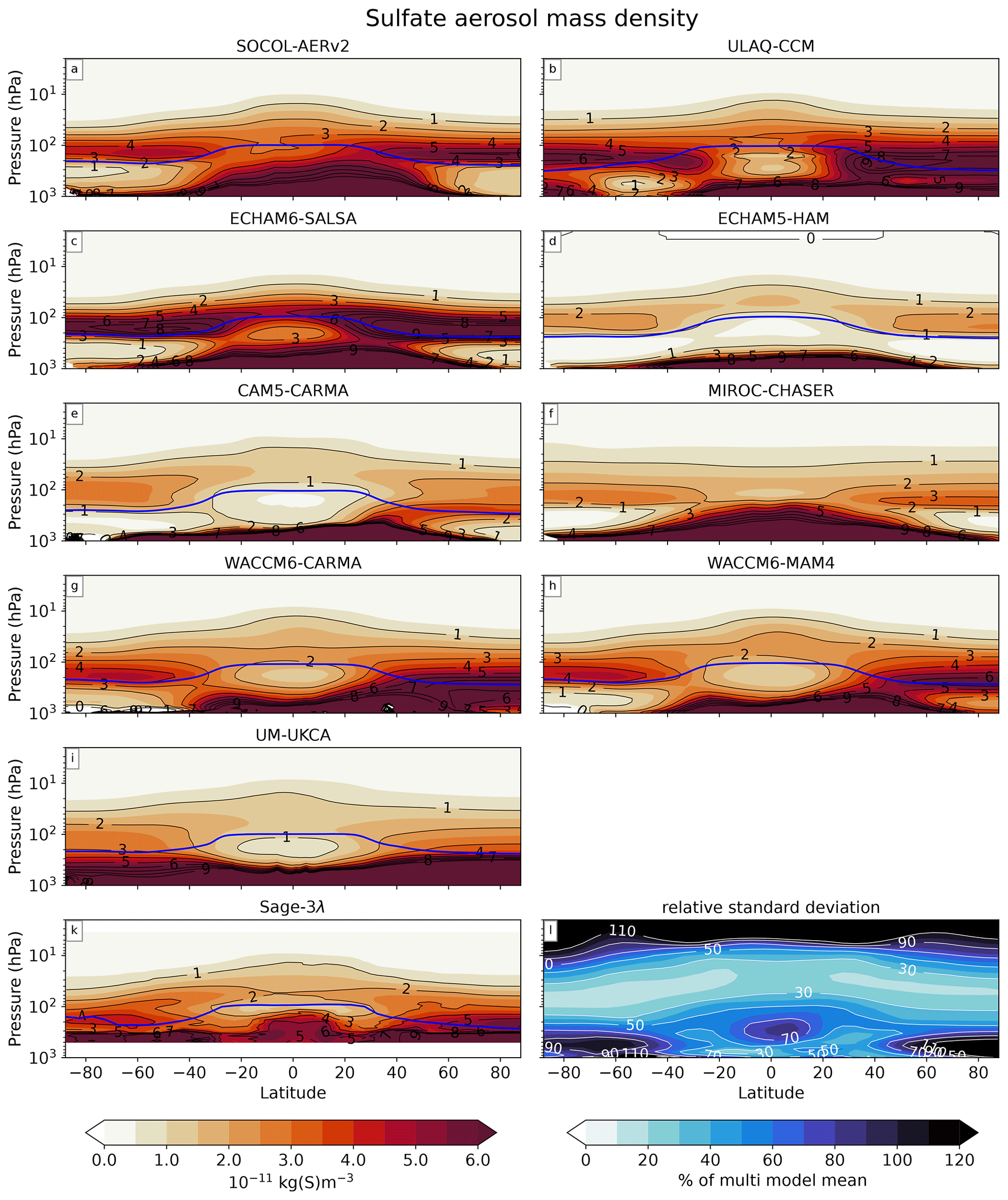
Figure 4 Stratospheric aerosol mass density (in kg (S) m⁻³) and averaged over the 20 simulation years (10 years for ULAQ–CCM) for each of the models (a–i) in comparison with 6 quiet years from 1999–2004 for SAGE-3λ (k). The dark blue lines are the time-averaged tropopauses in each respective model (a–i) and the ERA-I tropopause, using the World Meteorological Organization definition for SAGE-3λ (k). To obtain the mass density, we converted the mass mixing ratios of sulfate aerosol using the ideal gas law and provided temperature and pressure fields. Panel (l) shows the relative standard deviation as a percentage of the multi-model mean, where all model data were interpolated to 39 pressure levels and gridded onto a 5° × 5° grid.

In SAGE-3λ, the elevated values in the tropical troposphere are likely caused by minor volcanic eruptions. Kovilakam et al. (2020) mention four volcanic eruptions during 1999 and 2004: Ulawun (September 2000), Shiveluch (May 2001), Ruang (September 2002), and Reventador (November 2002). This last eruption emitted the largest amount of SO₂, with estimates by Carn (2022) at around 84 Gg, and a plume height of about 17 km or 94 Gg, reaching a plume height of about 22 km (Höpfner et al., 2015).

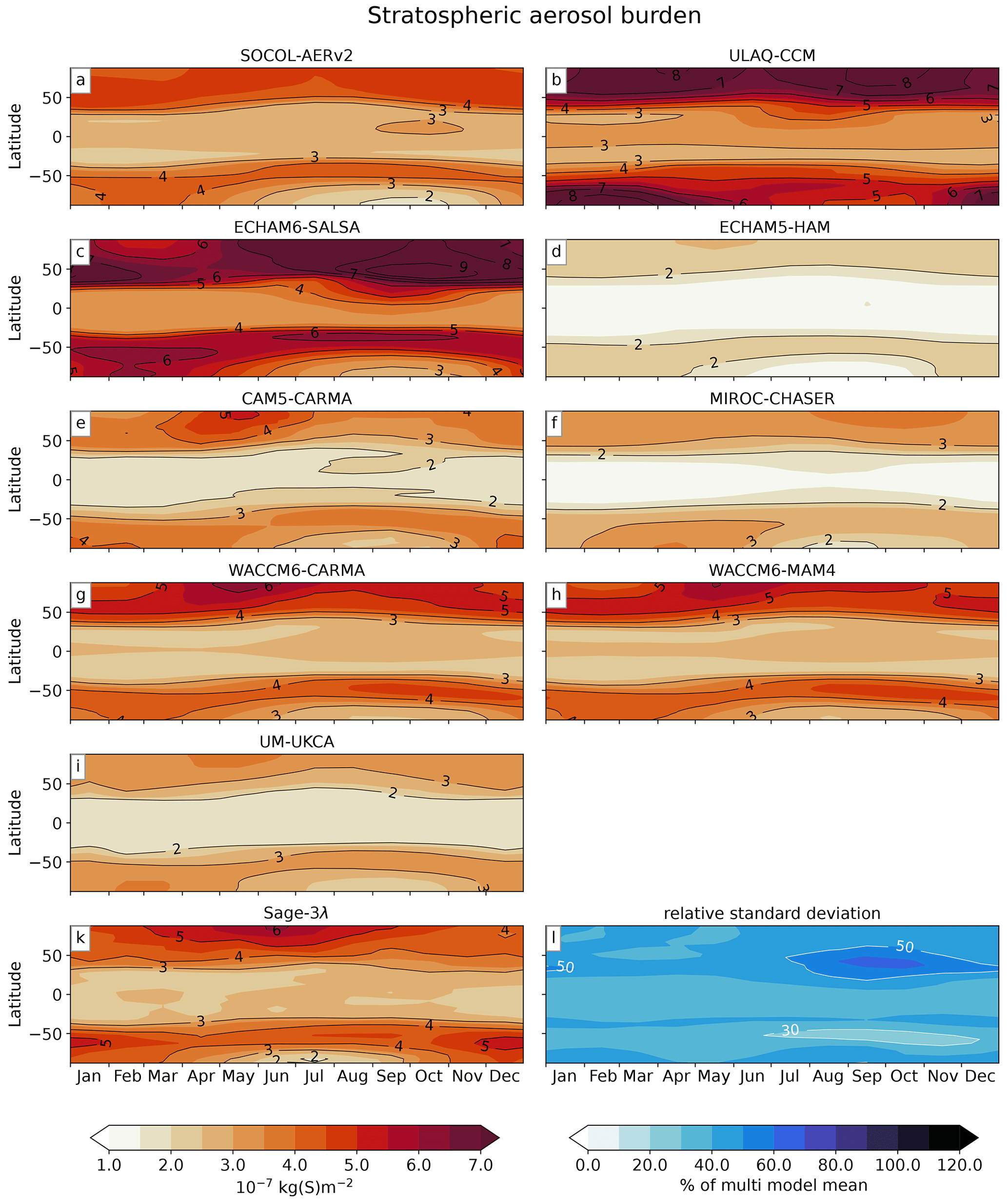
Figure 5 The stratospheric aerosol column (in kg m⁻²), averaged for each month over the 20 years of simulation, 10 years for ULAQ–CCM, and 6 years for SAGE-3λ. (a–i) Each panel represents one model for all latitudes over time. Panel (k) is the SAGE-3λ dataset. Panel (l) shows the RSD of all models (not including SAGE-3λ). All data were gridded to a 5° × 5° grid to calculate the RSD.

Considering only the stratosphere in Fig. 4, maxima are seen in the mid-latitudes and polar regions around the tropopause. Since emissions in the NH exceed those in the SH (Bates et al., 1992), and the stratospheric meridional transport from the tropics is weaker in the SH, the overall SH aerosol burden is also slightly lower in most models and in SAGE-3λ. Dynamical processes in the UTLS, such as isentropic mixing may have a strong influence on the stratospheric burden. The strongest maximum is seen in ULAQ–CCM (see also Fig. 3), with most of the aerosol residing above the tropopause. In all models, in the northern subtropical to mid-latitudes, the higher tropospheric burdens extend to higher altitudes, even “connecting” to the stratosphere. Yu et al. (2017) argued that 15 % of NH stratospheric aerosol originates from the Asian summer monsoon, where anthropogenic emissions are high (see also Fig. A1). Additionally, this could also be a result of higher emissions in the NH, coupled with generally higher convection above the continents (Takahashi et al., 2023) and isentropic transport and mixing with stratospheric air (Holton et al., 1995). As ULAQ–CCM has the lowest horizontal resolution, which leads to weakened transport barriers (Dietmüller, 2018) and stronger numerical diffusion, this effect could be a defining factor in this model. Another factor that could be responsible for the model biases is the climatology and variability in the tropopause. Figure A5 shows a high multi-model spread of the tropopause pressure, especially at high latitudes.

The seasonal cycle of the stratospheric aerosol burden is shown in Fig. 5. The main outliers in terms of absolute values are ULAQ–CCM, ECHAM6–SALSA, and ECHAM5–HAM, which is consistent with the values in Fig. 1. As in Fig. 3, the tropical region is marked by low values without an obvious seasonality. This is also evident from the RSD in Fig. 3l, with the lowest values in the tropics. Mid-latitude burdens coincide with the seasonal tropopause shift, where there is a sharp gradient towards the pole around 30°–50° N and S. In the SH, the highest burdens extend the furthest north to about 40° S in austral winter around August and September. In the NH, the pattern is not as smooth, and the RSD is also generally larger than in the SH. The largest RSD values lie in the northern mid-latitudes, while most other areas have an RSD of about 20 %–40 %. As already described in Fig. 4, this mirrors the higher tropospheric burdens at this latitude in ULAQ–CCM and is situated at the same time and place as the Asian summer monsoon (Yu et al., 2017). All models and SAGE-3λ show an aerosol minimum within the southern winter polar vortex due to the transport barrier in the winter and dominant downward transport within the vortex that brings sulfur-poor air from above. The RSD is higher in this region, possibly due to inter-model differences in vortex isolation.

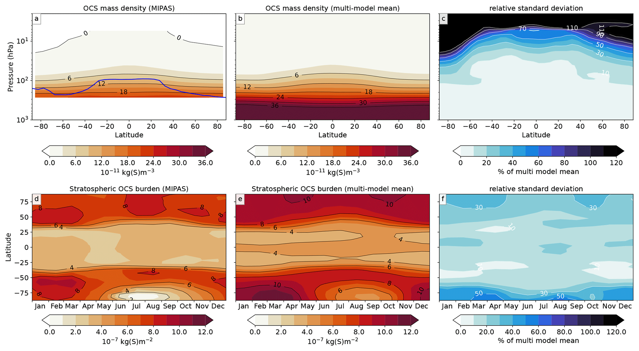
Figure 6 The OCS mass density (in kg (S) m⁻³) is shown in the top row (a–c). The bottom row depicts the zonally averaged stratospheric OCS burden (in kg (S) m⁻²) (d–f). Panels (a) and (d) show the MIPAS dataset, while panels (b) and (e) are the multi-model means, and panels (c) and (f) are the RSD. All model data were interpolated onto the same grid and vertical coordinates. The data were calculated from volume mixing ratios of OCS using the ideal gas law and provided temperature and pressure fields. ECHAM6–SALSA does not track OCS and is therefore not included here.

As the latitudinal distribution of OCS in Fig. 6 also shows a minimum within the SH polar vortex, we conclude that the model scatter is due to differences in the dynamics among models. The magnitude of the aerosol minimum varies little among models (Fig. 5l) and is also present in SAGE-3λ. Still, the timing of the vortex formation and breakup varies among models, and this has repercussions for aerosol transport. Rao and Garfinkel (2021) showed that the onset of the stratospheric final warming (SFW) tends to take place too late in many CMIP6 models in both hemispheres. WACCM- and MIROC-based models were part of this study, where the former tended to have a delayed SFW by up to 20 d, while MIROC tended to be much closer to the Japanese 55-year Reanalysis (JRA-55; Kobayashi et al., 2015; Rao and Garfinkel, 2021). In Fig. 5, we see that in WACCM6–CARMA and WACCM6–MAM4, SOCOL–AERv2, and CAM5–CARMA, for example, the aerosol is transported into the Antarctic region only in December, while this already takes place around November in ECHAM5–HAM, ULAQ–CCM, and UM–UKCA. In MIROC–CHASER, the transport seems to increase gradually over a longer period compared to other models, with values already increasing around September–October. In SAGE-3λ, the polar vortex aerosol minimum appears seasonally earlier in comparison to all models. From Fig. A3, which compares the zonal winds and temperature fields from the models to ERA-I data, it is evident that the southern winter polar vortex in WACCM6–CARMA and WACCM6–MAM4 is too strong in September–November (SON), while it is too weak (and warm) in ULAQ–CCM and ECHAM5–HAM. For the latter, this indicates an early onset of the SFW as opposed to WACCM6, where it takes place at a later time.

Larger differences are seen in the northern high to mid-latitudes, as already described in Sect. 3.2. Similar to the southern polar vortex, though much less pronounced, the northern polar vortex is marked by a local minimum in some models. This is only clear in ECHAM6–SALSA, CAM5–CARMA, WACCM6–CARMA, and WACCM6–MAM4. Although most models do depict a weak minimum, it is not well resolved in Fig. 5. From Fig. A3, we conclude that the northern polar vortex is too weak in ULAQ–CCM, while the signal is not as obvious in other models. A slightly stronger vortex is, for example, seen in ECHAM6–SALSA in December–February (DJF), while CAM5–CARMA, ECHAM5–HAM, and both WACCM6 models are slightly too cold in the lower and middle stratosphere. From March to May (MAM), the latter two have more pronounced northern polar vortices, indicating a generally delayed SFW, as with the southern polar vortex. For aerosol, this means too little transport into the polar region, resulting in a lower polar and higher mid-latitude optical depth.

3.3.2 Carbonyl sulfide

The vertical distribution of OCS is very similar in all models and the MIPAS observational data, with high burdens close to the surface and a relatively uniform gradient with height and much weaker latitudinal variation than for sulfate aerosol, as seen in the multi-model mean in Fig. 6. Averaging kernels were not considered here, which can improve the agreement of observations and model data, as shown in Glatthor et al. (2017). In the tropics, OCS is found at slightly lower pressures than at high and mid-latitudes, due to the vertical transport in this region (Plumb and Eluszkiewicz, 1999). Subsequently, OCS is oxidized and forms SO₂ at around 20 km (or ca. 60 hPa). Oxidation via O and OH only plays a minor role (Turco et al., 1979; Crutzen, 1976; SPARC, 2006). The low inter-model spread is also reflected in the RSD, with very low values in most of the troposphere. As the mass of OCS decreases, the RSD increases with height. In Fig. 6b, we see that the largest RSD values are in the stratosphere; although, at altitudes above 10 hPa, this can be disregarded as not much OCS is present there.

In terms of seasonality of the stratospheric burden, OCS showed similar issues to the ones that were discussed for sulfur in individual models in the previous section, though the RSD is generally smaller. It is the largest in the polar regions, which is strongly related to the differences in the tropopause (see Fig. A5). The tropopause in ULAQ–CCM extends lower in the polar regions than in other models, which with this uniform distribution of OCS allows more of it to reside in the stratosphere. This results in a pattern similar to sulfate in Fig. 4, where ULAQ–CCM has high burdens in the lower extratropical stratosphere, explaining its high total OCS burden in Fig. 1. Compared to MIPAS, the models behave very similarly, whereas again the minimum in the SH polar vortex is earlier and more pronounced in the observations compared to the multi-model mean.

3.3.3 Sulfur dioxide

SO₂ mass density is largest in the lower troposphere and the UTLS and decreases in the higher stratosphere (Fig. 7). In some models, higher SO₂ values can also be seen in the tropical free troposphere. SO₂ burdens are higher directly below rather than above the tropical tropopause, which is opposite to the behavior of the aerosol burden in Fig. 4, as a result of the conversion of SO₂ to H₂SO₄, and subsequently sulfate, during the vertical transport of air in this region. Similar to Fig. 4, higher SO₂ values reach up to the tropopause in most models north of about 30° N. This is again a result of anthropogenic SO₂ emissions in this area, as shown in Fig. A4a–f. In REF, more SO₂ is transported to the stratosphere in many models. In ULAQ–CCM, WACCM6–CARMA, and WACCM6–MAM4, for example, the lowermost stratospheric SO₂ mixing ratio is increased by 50 % to up to 80 %, due to anthropogenic emissions. In contrast, in ECHAM5–HAM and MIROC–CHASER, most of these emissions do not reach the stratosphere. This then results in the inter-hemispheric asymmetry between the models in terms of the lower stratospheric SO₂.

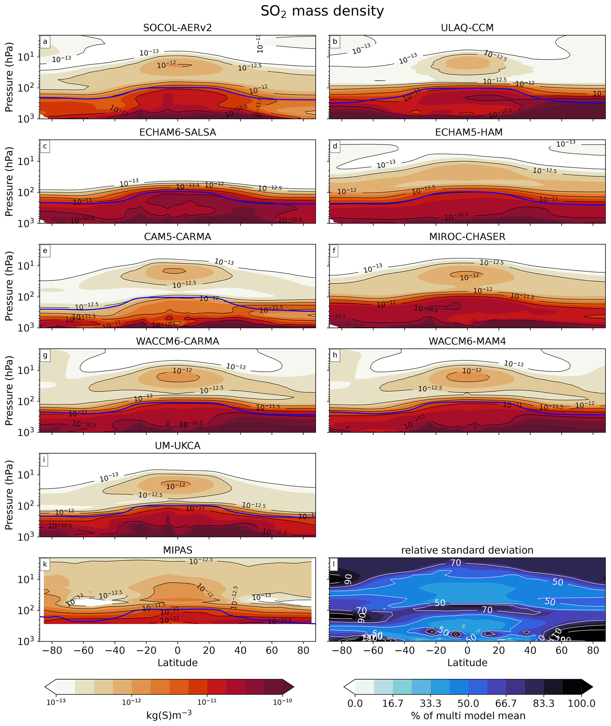
Figure 7 The stratospheric SO₂ burden (in kg (S) m⁻³) on a logarithmic color scale. The models are depicted (a–i), while the MIPAS-derived dataset is shown (k). The RSD (l) is obtained from the multi-model ensemble. The tropopause is shown as a blue line and was averaged over the simulated time period and all longitudes. The mass density was obtained from volume mixing ratios, using the model temperature and pressure applied to the ideal gas law.

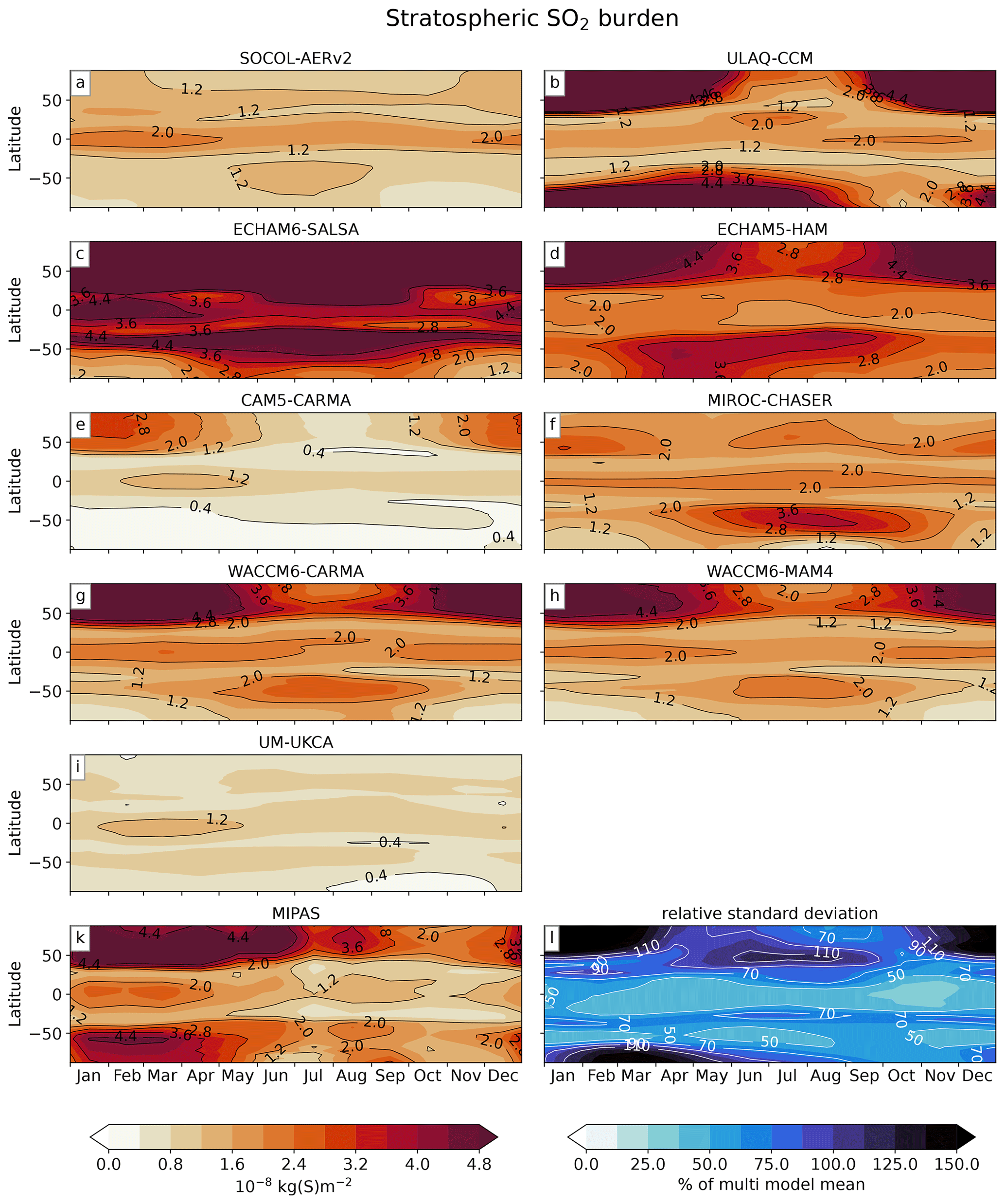
Figure 8 The stratospheric SO₂ burden (in kg (S) m⁻²) for all models (a–i), MIPAS (k), and the multi-model RSD (l). See also Fig. 5.

Although MIPAS (Fig. 7k) has a distribution more similar to, e.g., ECHAM6–SALSA than the models with lower stratospheric SO₂ burdens, the values in Fig. 1 are closer to, e.g., WACCM6–CARMA. In the stratosphere, most models and MIPAS have a secondary maximum of SO₂ in the tropical region between about 10-20 hPa. This can be attributed to the photolysis of OCS, discussed in the previous section, as well as to the evaporation of aerosol and subsequent photolysis of H₂SO₄ (Turco et al., 1979). In MIPAS, we see an increase in SO₂ above 40 hPa, even outside the tropics, which is not seen in any of the models to the same extent. This is attributed to H₂SO₄ photolysis, which could be underestimated in models (Höpfner et al., 2013; Sheng et al., 2015; Brühl et al., 2015). As ECHAM6–SALSA does not include OCS, SO₂ only resides in the lower stratosphere. The other extreme is seen in ECHAM5–HAM, where too little SO₂ may be oxidized due to low OH concentrations (see Sect. 3.2). Therefore, the lifetime of SO₂ increases, and there is more of it available to be further transported toward the poles from the tropics. The RSD in Fig. 7l is the highest in the UTLS and the northern extratropical troposphere, indicating low agreement among models in these regions. Models agree the most in the free tropical troposphere and the lower tropical stratosphere. Above 30 hPa, the RSD again increases, indicating differences in how models behave at the upper edge of the Junge layer both in terms of microphysics and photolysis.

Figure 8 shows the stratospheric SO₂ burden distributions. As for OCS in Figs. 5 and 6, the models follow a similar seasonal pattern in which the tropical region can be clearly distinguished from the extratropics. However, for SO₂, the lowest burdens are not found in the tropical region for all models. Instead, in CAM5–CARMA, the SH has lower burdens, while in most other models, these lower burdens are mainly seen in polar summer (except for ULAQ–CCM and UM–UKCA). Lower burdens are seen in the SH for most models, though still often exceeding the tropical burdens for several months, as in ECHAM5–HAM, WACCM6–MAM4, WACCM6–CARMA, and MIROC–CHASER. As described above, the higher burdens in ECHAM5–HAM, ECHAM6–SALSA, and ULAQ–CCM are found in the extratropical region. In WACCM6–CARMA and WACCM6–MAM, whose stratospheric SO₂ burdens were in the middle range, only the NH is characterized by higher burdens. While the higher SO₂ burdens in ECHAM5–HAM were previously explained by lower OH burdens, the higher SO₂ burdens in ECHAM6–SALSA and ULAQ–CCM can now be explained by increased transport across the tropopause in the northern subtropical region. While the differences among models are considerable, the best agreement outside the tropics is found from November to December at southern high latitudes (Fig. 8l).

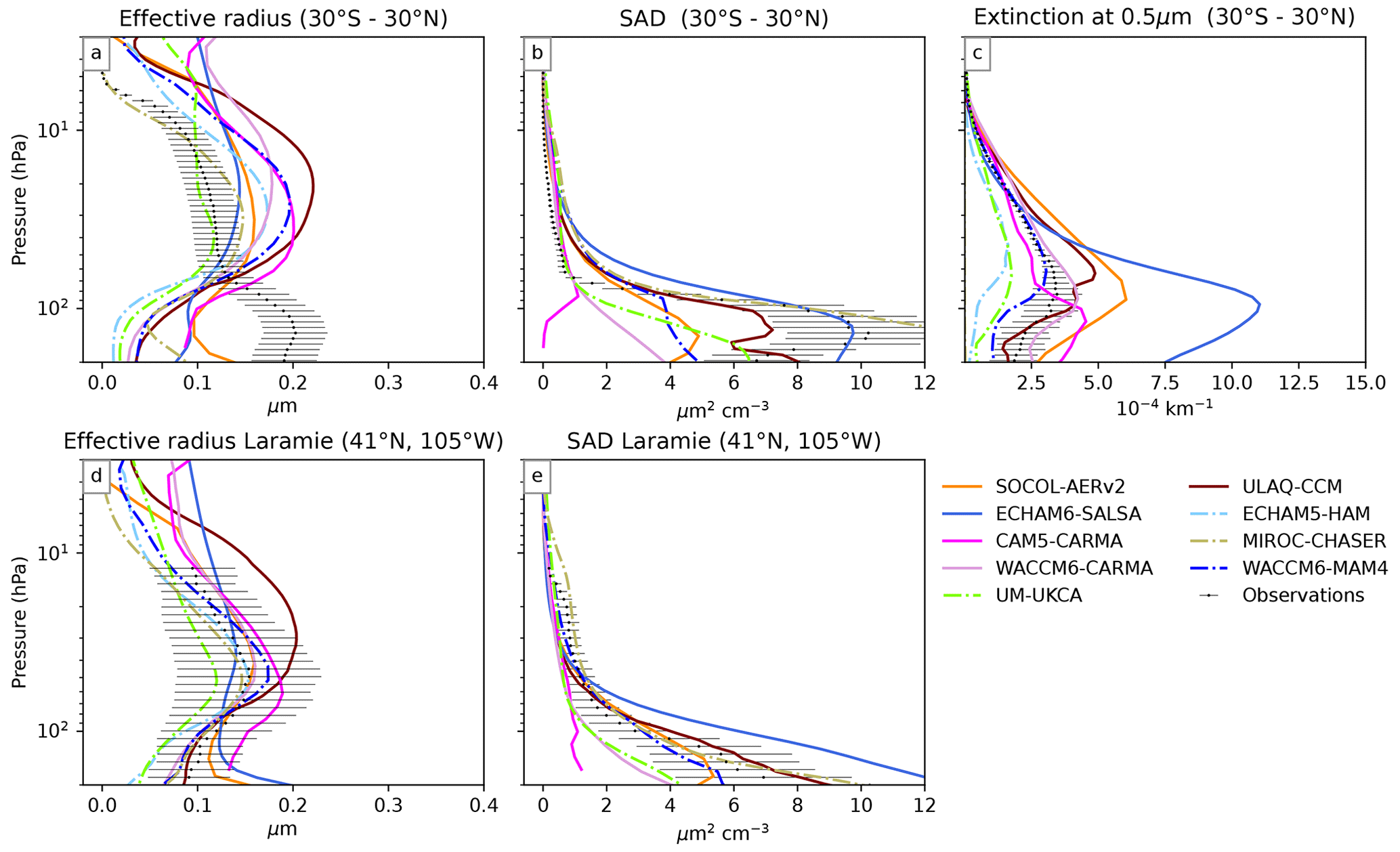
Figure 9 The effective radius, SAD, and extinction for each model in the tropical region (30° N to 30° S) and in a single grid cell at Laramie (41° N, 105° W). Additionally, we show the effective radius and surface area density for SAGE II (observations in panels (a) and (b) and the extinction from GloSSACV2.2 in panel (c)). Observations in panels (d) and (e) are derived from OPC measurements. Models with sectional aerosol schemes are shown as solid lines, while modal aerosol schemes are dash-dotted lines. Extinction in SOCOL–AERv2, ULAQ–CCM, and MIROC–CHASER is at 525 nm; in CAM5–CARMA at 532 nm; in ECHAM6–SALSA at 533 nm; and in ECHAM5–HAM, WACCM6–CARMA, WACCM6–MAM4, and UM–UKCA at 550 nm. We use the effective radius of pure sulfate for SOCOL–AERv2 and ULAQ–CCM, an SAD-weighted average of pure sulfate and mixed aerosol effective radius for CAM5–CARMA and WACCM6–CARMA and the effective radius of all aerosol for ECHAM6–SALSA, ECHAM5–HAM, WACCM6–MAM4, and MIROC–CHASER. SAD describes only pure sulfate in SOCOL–AERv2, ULAQ–CCM, and CAM5–CARMA, while it encompasses all aerosol in ECHAM6–SALSA, ECHAM5–HAM, WACCM6–MAM4, and MIROC–CHASER. In WACCM6–CARMA, SAD is summed up for pure sulfate and mixed aerosol. Extinction of pure sulfate is used in SOCOL–AERv2 and ULAQ, while it is summed up for pure sulfate and mixed aerosol in WACCM6–CARMA, and for all remaining models, it is the total extinction.

3.4 SAD and effective radius

Figure 9a and d show the simulated effective radius, surface area density (SAD; Fig. 9b and e), and extinction in the tropics in (Fig. 9c), averaged over the whole time period; for the first two aerosol variables, values measured at Laramie, Wyoming (41° N, 105° W), are also shown. In the models, the closest grid box to Laramie was selected for comparison to the balloon observations. The effective radius in Fig. 9a increases above 100 hPa and reaches a maximum at around 20–30 hPa, ranging from about 0.12 µm (UM–UKCA) to 0.22 µm (ULAQ–CCM). At Laramie, this maximum is found at slightly lower altitudes at 40–60 hPa in all models, except ECHAM6–SALSA and ULAQ–CCM. While ULAQ–CCM and UM–UKCA are still outliers, all other models are closer together in this region in terms of their effective radius. In Sect. 3.2, we suggest that the size distribution is the cause of differences in SAOD between WACCM6–CARMA and WACCM6–MAM4, despite very similar burdens. Figure 9 confirms that the effective radius is larger in WACCM6–MAM4 (below ca. 15 hPa), while its extinction is lower than in WACCM6–CARMA. This is also seen at Laramie in Fig. 9d, although to a lesser extent. The SAGE-II-derived data indicate a smaller effective radius than in the models, except for MIROC–CHASER at this altitude, while exceeding the models' effective radius at lower levels. However, we have to stress that Quaglia et al. (2023) did not use the SAGE II data below 21 km (or ca. 50 hPa), due to the lower quality of the data at lower altitudes. Additionally, when the aerosol is low, particularly in background conditions, the SAGE-II-derived data and optical particle counters deviate significantly from each other (Kovilakam and Deshler, 2015). When comparing to the OPC measurements at Laramie, we also see a much better agreement with the models than with the SAGE II data in the tropical region. Quaglia et al. (2023) showed a distribution of effective radii in the pre-Pinatubo quiet conditions ranging from 0.1 µm in SOCOL–AERv2 to 0.17 µm in ECHAM6–SALSA and 0.27 µm in ULAQ–CCM. In our study, however, ECHAM6–SALSA has the smallest effective radius out of these three models. In direct comparison with the volcanically perturbed values in Quaglia et al. (2023), we see that the maximum effective radius is reduced to about half during these quiet conditions.

SAD is marked by a larger disagreement between the models, reflecting the differences among burdens described in Sect. 3.1. At 70 hPa, SOCOL–AERv2, ULAQ–CCM, WACCM6–MAM4, and MIROC–CHASER are closest to the observation-derived data by SAGE II, although the latter shows a sharper decrease towards 60 hPa, where WACCM6–CARMA, WACCM6–MAM4, and CAM5–CARMA are closer. Again, more models are closer to the OPC observations in mid-latitudes in Fig. 9e than to observations in Fig. 9b. In Fig. 9b, SAD in CAM5–CARMA and WACCM6–MAM4 decreases rapidly around 80 hPa, consistent with lower aerosol burdens in the upper tropical troposphere. In CAM5–CARMA, the SAD decreases to 0, as this variable is not defined below the tropopause.

Differences among models are again very large, concerning both the altitude and magnitude of the maximum extinction in the stratosphere (see Fig. 9c). While in CAM5–CARMA the maximum extinction is slightly below the tropopause (at ca. 100 hPa), it is above the tropopause for most other models. In MIROC–CHASER again, the stratospheric values are very low throughout and only increase in the troposphere. The largest stratospheric extinction coefficients are seen in ECHAM6–SALSA, which is consistent with the higher burdens in this model, followed by SOCOL–AERv2 and ULAQ–CCM. CAM5–CARMA and both WACCM6 models have mid-range values, consistent with GloSSACV2.2, while ECHAM5–HAM has the lowest extinctions, also consistent with its overall aerosol burdens. In Quaglia et al. (2023), the extinction coefficients also vary a lot among models for volcanically perturbed conditions.

4 Conclusions

In this study, we present an analysis of the atmospheric sulfur budget using nine state-of-the-art global circulation models with interactive aerosol modules and sulfur chemistry. In particular, we showcase the burdens of the main sulfur species represented in these models (OCS, sulfate aerosols, and SO₂), as well as their latitudinal and vertical distribution and seasonal variability. Emission and deposition fluxes are also discussed. Sulfate aerosol, OCS, and SO₂ behave very differently in the atmosphere, providing insight into the modeled processes. OCS is almost chemically inert in the troposphere and is primarily influenced by transport mechanisms but undergoes photolysis in the stratosphere. Conversely, SO₂, which has a lifetime of a few days to a few weeks, is more responsive to chemical processes in the troposphere.

Previous studies have revealed the main sulfur species abundant in the atmosphere to be OCS, SO₂, and sulfate aerosol, which we here find to make up about 95 % of the total tropospheric and 98 % of the stratospheric sulfur mass, averaging over all models which include these three species. However, variability across models in the stratospheric burden of each of these main species is large, with burdens of 319 ± 50 Gg (S) for OCS, 12 ± 7 Gg (S) for SO₂, and 156 ± 51 Gg (S) for sulfate aerosol. Anthropogenic emissions of SO₂ dominate the sulfate aerosol burden in the NH troposphere and increase the aerosol mass in the lowermost stratosphere by 10 %–80 %, which is very model-dependent. The SH, both in the troposphere and the stratosphere, is less affected by anthropogenic activity (10 %–30 %). The total deposition varies across models by about a factor of 2 between 99 692 and 51 211 Gg (S) yr⁻¹ (or 86 693 ± 18 115 Gg (S) yr⁻¹). Models also disagree on the form in which sulfur is deposited, as well as the split between wet and dry deposition. More sulfur being deposited as aerosol precursor gases could lead to a lower aerosol burden, as discussed by Textor et al. (2006). We do, however, not explicitly observe such behavior. Furthermore, the relative importance of wet and dry deposition is expected to depend on the solubility of the compound, as well as the treatment of clouds and precipitation in the respective models (Textor et al., 2006). Evaluating model performances with respect to clouds and precipitation is beyond the scope of this study, and we refer to each model's documentation for details, as well as to dedicated model intercomparison activities on this topic (e.g., Webb et al., 2017).

In terms of the spatial distribution, the models agree very well on the distribution and seasonality in the SH for all species. However, in the NH, where anthropogenic emissions contribute significantly to the aerosol burden, especially at low to mid-latitudes, more uncertainties persist. This is in part due to dynamical uncertainties in the northern polar vortex (Karpechko et al., 2022) affecting the transport into high latitudes. The highest values in the northern extratropics are seen in ULAQ–CCM, which are associated with a slower and warmer vortex compared to the other models. Additionally, resolution-dependent isentropic transport through the subtropical tropopause (Holton et al., 1995; Gettelman et al., 2011) could play a major role in increasing the extratropical burdens of OCS and sulfate in some models, which may be even more pronounced during the Asian monsoon, during which aerosol transport to the stratosphere is facilitated (Yu et al., 2017). A low horizontal resolution also increases diffusion across transport barriers, such as the polar vortex or the tropopause, where it crosses the isentropes in the subtropics (Dietmüller, 2018). The speed of the BDC also could be a major factor of uncertainty (Abalos et al., 2021) affecting both the transport through the shallow branch, as well as upwelling, and thus the confinement of aerosol in the tropics. Idealized tracer experiments using SO₂ emissions might help to isolate the dynamical biases.

The analysis on the effective radius, SAD, and extinction in the tropics and at Laramie reveals notable differences among models. While the effective radius shows some agreement among models and is within the uncertainty in the OPC measurements in Laramie in all models, SAD exhibits larger discrepancies, reflecting the variations in aerosol burdens. Extinction levels also vary significantly, with ECHAM6–SALSA showing the highest values. Elaborating further on the reasons for the size distribution uncertainties would require a closer look at the individual microphysical processes, as was also highlighted by Quaglia et al. (2023), but such data were not available in most of the models in our study. Recently, concerns have arisen regarding nucleation schemes, such as Vehkamäki et al. (2002), which may overestimate the nucleation of new particles (Laakso et al., 2022; Yu et al., 2023). However, these studies focus on stratospheric aerosol injection scenarios, where sulfur is much more abundant than in the background conditions presented in this study. Using observational data, Wrana et al. (2023) showed that small volcanic eruptions affect the background size distribution of aerosols in unexpected ways, sometimes decreasing instead of increasing the effective radius. The volcanic events highlighted there can be further used as model test cases, contributing knowledge to the model performance in terms of microphysics and its dependence on the background conditions.

With this study, we have provided a first multi-model analysis of the background burdens of sulfur in atmospheric models. We mainly assessed the burdens and latitudinal and vertical distributions of sulfur species, allowing us to identify potential reasons for model diversity. As burdens are merely the result of fluxes, the next step would be to compare chemical and microphysical fluxes, as well as emission, cross-tropopause, and deposition fluxes. For SO₂ in particular, cross-tropopause fluxes in the mid-latitudes have the potential to provide more insight into the underlying processes causing differences in stratospheric burdens.

Overall, this study sheds new light on the atmospheric sulfur budget and, for the first time, presents it in a multi-model context. Our results highlight the importance of an interplay between the chemical, microphysical, and dynamical processes in atmospheric models. The interdependence of these processes complicates the attribution of biases when looking only at their final products, namely the distribution and variability in sulfur species in the atmosphere. The same holds true for the recent similar studies focused on volcanic events (e.g., Quaglia et al., 2023; Clyne et al., 2021; Marshall et al., 2018) and stratospheric aerosol injections (e.g., Weisenstein et al., 2022). Some conclusions could be drawn by relating different variables. However, more detailed investigations of the reasons for inter-model disagreement would require process-oriented experiments such as the sensitivity experiments proposed by ISA–MIP for the Pinatubo eruption in the Pinatubo Emulation in Multiple models (PoEMS) (e.g., Timmreck et al., 2018). However, these experiments still include the full range of complexity and may therefore be difficult to interpret. Much more illuminating would be experiments in which the degrees of freedom are reduced so that specific questions can be addressed. Comparison of standalone parts of the respective model codes, i.e., box model versions of the microphysical and chemical schemes, short and long wavelength radiative transfer modules, and treatment of the Mie calculation, is one possible solution. The other would be to perform dedicated tracer studies or simple sulfur cycle experiments (with a prescribed aerosol size distribution). Revisiting the ISA–MIP experiments in this sense and developing a set of dedicated benchmark simulations related to available observations would therefore be a valuable next step to validate and improve global stratospheric aerosol models but also to reduce uncertainties in solar radiation modification scenarios.

Appendix A

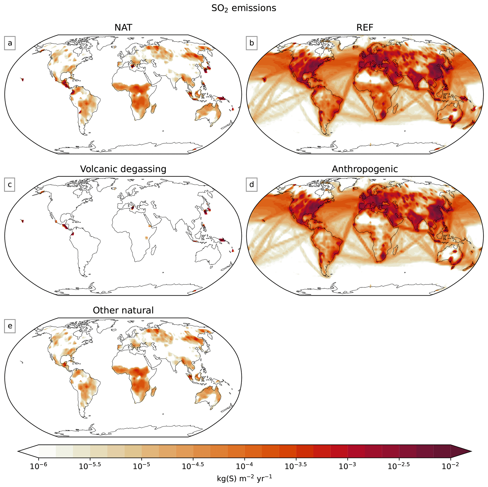
Figure A1 The SO₂ emissions in the NAT (a) and REF (b) experiments. NAT is composed of volcanic outgassing (c) and biomass burning (e), while the REF experiment additionally includes anthropogenic emissions (d).

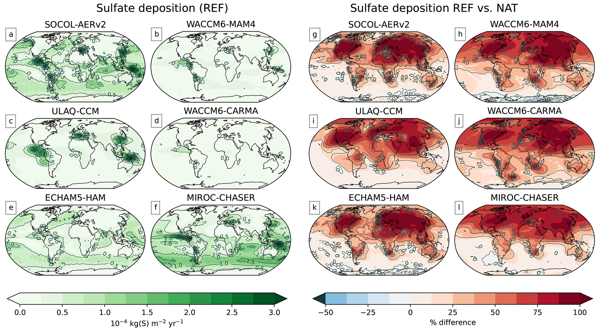
Figure A2 Total deposition fluxes of sulfate aerosol (as a sum of dry and wet deposition) as absolute values are given in panels (a)–(f) and as a percent difference between the REF and NAT experiments in panels (g)–(l). The percent difference is calculated as REF–NAT and divided by REF. The data are time-averaged over the whole time period.

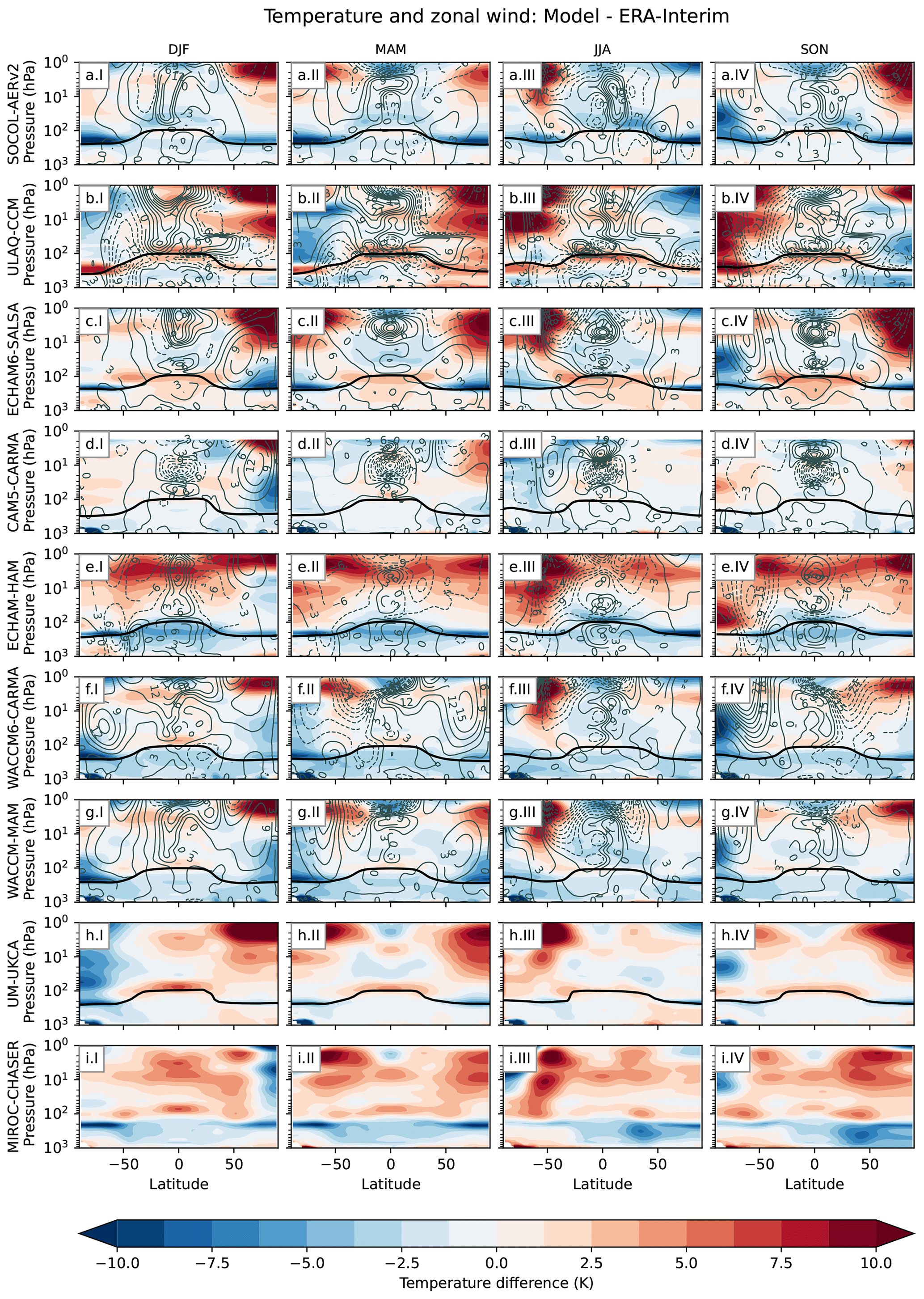
Figure A3 The difference in the time slice simulations averaged over 20 years for each season for temperature and zonal winds. Anomalies are calculated with respect to 1999–2004 ERA-I data, which was regridded to the respective model grid. Temperature is shown in color, while winds are in gray contours. Solid lines indicate stronger-than-observed westerly zonal winds, while dashed lines are weaker than observed. The numbers along with the contours are the anomalies (in m s⁻¹). Each column represents one season, while each row represents one model. The simulated tropopause is shown as a black line, also averaged over each season, respectively.

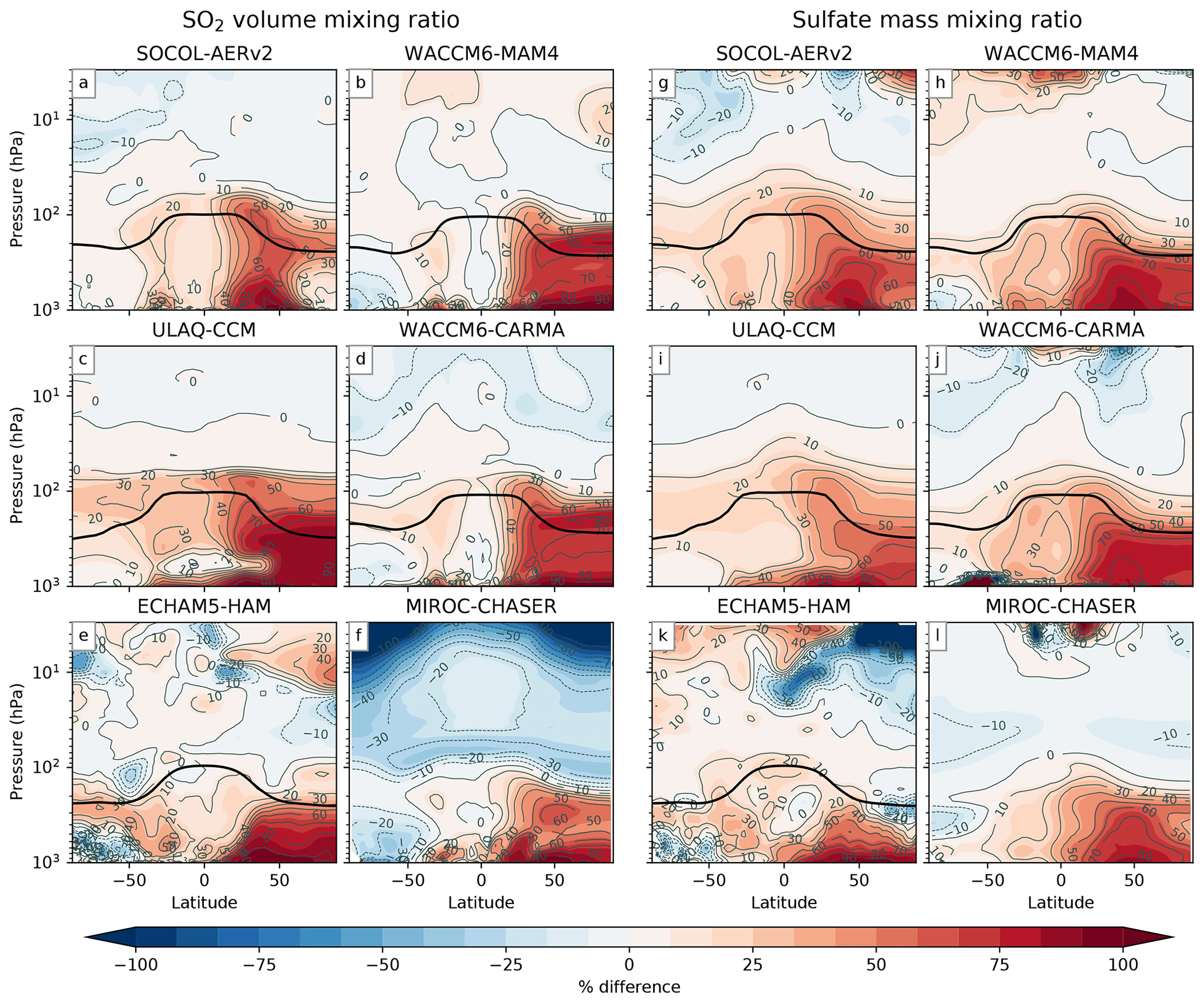
Figure A4 The percent difference between the REF experiment and the NAT experiment of the SO₂ volume mixing ratio in panels (a)–(f) and the sulfate mass mixing ratio in panels (g)–(l). The percent difference is calculated as REF–NAT divided by REF. All data are zonally averaged and over the whole time period of each simulation.

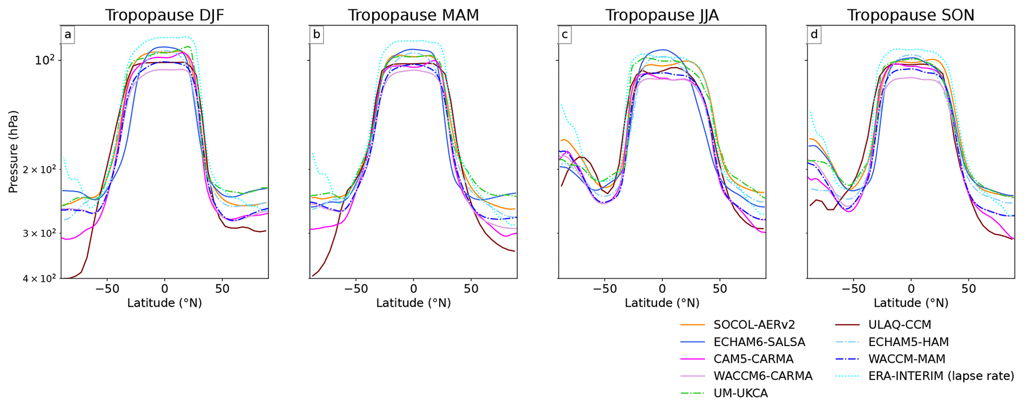
Figure A5 The tropopauses of each model, as well as the ERA-I-derived tropopause, which was used to calculate stratospheric burdens for SAGE-3λ.