A novel method for detecting tropopause structures based on the bi-Gaussian function

The tropopause is an important transition layer and can be a diagnostic of upper-tropospheric and lower-stratospheric structures, exhibiting unique atmospheric thermal and dynamic characteristics. A comprehensive understanding of the evolution of fine tropopause structures is necessary and primary for the further study of complex multi-scale atmospheric physical–chemical coupling processes in the upper troposphere and lower stratosphere. A novel method utilizing the bi-Gaussian function is capable of identifying the characteristic parameters of vertical tropopause structures and providing information on double-tropopause (DT) structures. The new method improves the definition of the cold-point tropopause and detects one (or two) of the most significant local cold points by fitting the temperature profiles to the bi-Gaussian function, which defines the point(s) as the tropopause height(s). The bi-Gaussian function exhibits excellent potential for explicating the variation trends of temperature profiles. The results of the bi-Gaussian method and lapse rate tropopause, as defined by the World Meteorological Organization, are compared in detail for different cases. Results indicate that the bi-Gaussian method is able to more stably and obviously identify the spatial and temporal distribution characteristics of the thermal tropopauses, even in the presence of multiple temperature inversion layers at higher elevations. Moreover, 5 years of historical radiosonde data from China (from 2012 to 2016) revealed that the occurrence frequency and thickness of the DT, as well as the single-tropopause height and the first and second DT heights, displayed significant meridional monotonic variations. The occurrence frequency (thickness) of the DT increased from 1.07 % (1.96 km) to 47.19 % (5.42 km) in the latitude range of 16–50° N. The meridional gradients of tropopause height were relatively large in the latitude range of 30–40° N, essentially corresponding to the climatological locations of the subtropical jet and the Tibetan Plateau.

1 Introduction

As a pivotal transitional layer uniting the troposphere and stratosphere, the tropopause layer is subject to complex multi-scale atmospheric physical–chemical coupling processes, such as atmospheric radiation and dynamical processes (Fueglistaler et al., 2009; Gettelman et al., 2011). The tropopause is a transitional layer between the upper troposphere and lower stratosphere (UTLS), mainly manifesting in the transportation of atmospheric energy and masses to the stratosphere, thereby serving as a “gate” for further advection and diffusion (Yang and Lv, 2004; Fueglistaler et al., 2009; Holton et al., 1995). Long-term variations in the tropopause's thermal and dynamic structures are regarded as crucial indicators of climate change (Santer et al., 2003a, b; Sausen and Santer, 2003; Xian and Fu, 2017; Seidel et al., 2001; Shepherd, 2002; Seidel and Randel, 2006; Thompson et al., 2021; Meng et al., 2021). However, the comprehension of fine tropopause structures is still limited (Bian et al., 2020), leading to varying degrees of bias in the analysis of tropopause inversion layer characteristics (Randel et al., 2007b; Wang et al., 2013) and in climate model simulations (Li et al., 2020; Sun et al., 2021; Tian et al., 2017; Xian and Fu, 2015; Maddox and Mullendore, 2018).

It is beneficial to understand the formation mechanisms of the tropopause through a combination of tropospheric and stratospheric processes and to further research stratosphere–troposphere exchange (STE) processes by defining the tropopause from various perspectives. Reviews of existing tropopause definitions and their performances were summarized by Maddox and Mullendore (2018), Tinney et al. (2022), and Boothe and Homeyer (2017). In early atmospheric models, the tropopause was characterized as a discontinuous interface featuring a sharp vertical gradient. Reed (1955) proposed the concept of the dynamic tropopause and discovered tropopause-folding events. Later, the dynamic tropopause was defined based on the zero-order discontinuity of potential vorticity (Danielsen et al., 1987). Based on the vertical structure of atmospheric temperature and the characteristics of a sharp decrease in the temperature lapse rate, the World Meteorological Organization (WMO) defined the lapse rate tropopause (LRT) (WMO, 1957). From a chemical point of view, Bethan et al. (1996) analyzed whether there was a saltus in the atmospheric tracer concentrations across the thermal and dynamic tropopause and set a threshold for the vertical gradient of the ozone mixing ratio to represent the ozone tropopause (Pan et al., 2004, 2014; Ma et al., 2022). Recently, a stability-based definition of the potential-temperature-gradient tropopause (PTGT) was developed to identify the greatest composition change within the tropopause transition layer (Tinney et al., 2022).

It is more reasonable to consider the tropical tropopause as a transition layer than a discontinuous interface (Highwood and Hoskins, 1998). Gettelman and Forster (2002b) comprehensively considered both radiation and convection, using the cold-point tropopause (CPT) and the potential-temperature lapse rate minimum (LRM) tropopause as the upper and lower boundaries of the tropical tropopause layer, respectively. A primary characteristic of the tropopause is the drastic alteration of atmospheric static stability that occurs when crossing this transitional layer. To estimate the thickness of the tropopause layer, a parameter for atmospheric static stability – buoyancy frequency (N) – has been used, characterized by the vertical potential-temperature gradient (Homeyer et al., 2010). Static stability undergoes a discrete jump from a low value (unstable) in the troposphere to a high value (stable) in the stratosphere (Birner, 2006; Gettelman and Wang, 2015; Bai et al., 2017).

The meridional distribution of the height of the thermal tropopause, ranging from tropical to subtropical latitudes, often exhibits a discontinuous variation known as the “tropopause break” (Randel et al., 2007a; Rieckh et al., 2014; Schmidt et al., 2004; Palmen, 1948; Xian and Homeyer, 2019). Coincidentally, at overlapping tropical and middle–high latitudes adjacent to the subtropical jet (STJ), double tropopauses (DTs) are frequently formed (Randel et al., 2007a; Xian and Homeyer, 2019; Schmidt et al., 2006). Fluctuations in atmospheric temperature resulting from different atmospheric circulation systems, such as the Asian summer monsoon and polar vortex, can cause abnormal changes in tropopause height and increase the possibility of DT formation (Randel et al., 2007a; Rieckh et al., 2014; Ravindrababu et al., 2020; Shangguan et al., 2019). Some studies have focused on atmospheric stability and STE processes associated with DT events, revealing that convective overshooting can impact the maximum water vapor levels and stratospheric hydration in the lower stratosphere, as well as the ozone concentration (Randel et al., 2007a; Pan et al., 2004; Gamelin et al., 2022; Homeyer et al., 2014a, b). The DT has an important influence on the vertical distribution, transport, and diffusion of atmospheric constituents and is a key non-negligible transition layer when considering any mid-latitude stratosphere–troposphere activities (Peevey et al., 2014; Parracho et al., 2014; Liu and Barnes, 2018).

In order to deeply understand the coupling processes and triggering mechanisms involved in the UTLS, the evolution of fine tropopause structures must be comprehensively understood. However, the results of existing tropopause identification methods are quite different in some cases, and the formation mechanisms and evolution processes of the DT and the tropopause inversion layer are still active areas of research. Therefore, it is imperative to find a reliable and highly universal method to identify the characteristic parameters of vertical tropopause structures (Bian et al., 2020; Tian et al., 2017).

The objective of this study is to introduce a new method for identifying the multiple characteristic parameters of vertical tropopause structures. Temperature profiles obtained from radiosondes have been fitted using the bi-Gaussian function, which can not only identify the height and temperature of the tropopause but also convey information about the DT structure, such as its thickness, while effectively assisting in the characteristic analysis of the tropopause inversion layer. The key aspects of this work are outlined as follows. Section 2 presents an account of the historical radiosondes used in the study, commonly utilized definitions of the thermal tropopause from previous research, and a thorough description of the new identification method based on the bi-Gaussian function. A feasibility analysis of the new method and comparisons with existing definitions are highlighted in Sect. 3. Section 4 provides a comprehensive discussion of the spatiotemporal characteristics of tropopause structures in China, based on this new bi-Gaussian method. Ultimately, conclusions are summarized in Sect. 5.

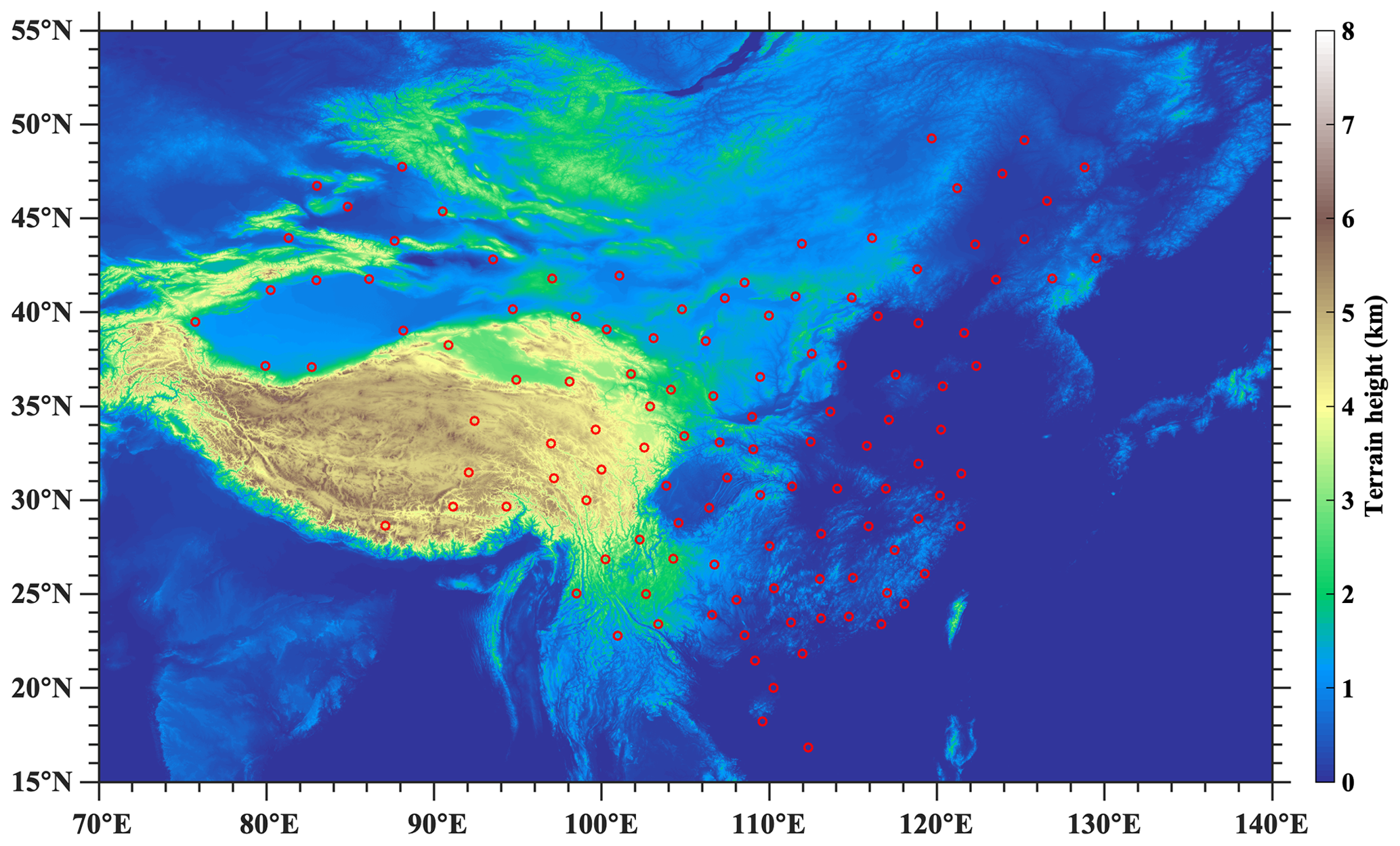
Figure 1 The geographical locations of sounding sites (red circles) and relevant terrain heights.

2 Data and methods

2.1 Radiosondes

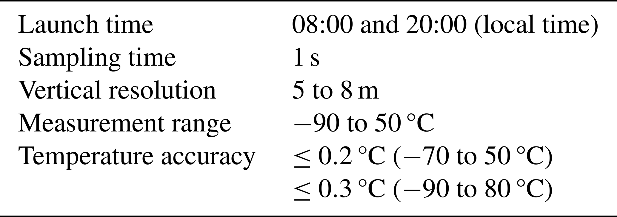
Despite numerous studies on tropopause structures based on satellite data (Alexander et al., 2011; Liu et al., 2019; Rieckh et al., 2014), radiosonde observations of air temperature – traditionally the most widely used method – are crucial for studying fine tropopause structures (Chen et al., 2006; Xian and Homeyer, 2019; Seidel et al., 2001). Historical radiosonde data were obtained from 120 sounding sites in China (color-coded in Fig. 1), covering tropical, subtropical, temperate, and plateau climate zones from 2012 to 2016, as described in detail in Guo et al. (2016). Once- or twice-daily radiosondes, launched at 08:00 and 20:00 (local time) throughout the four seasons, have a higher vertical resolution (about 5 to 8 m) than reanalyses, providing an excellent opportunity for the more precise identification of tropopause height, tropopause temperature, and DT structures. Basic information on the temperature profiles from the radiosondes is listed in Table 1. A 15-point running mean was adopted for the temperature and potential-temperature profiles.

Table 1 Information from high-resolution temperature profiles for radiosonde measurements.

2.2 Previous definitions of the thermal tropopause

Five definitions of the thermal tropopause (concerning the CPT, LRT, LRM, PTGT, and curve fit to N²) are shown in Fig. 2, using radiosonde data from a tropical site (16.83° N, 112.33° E).

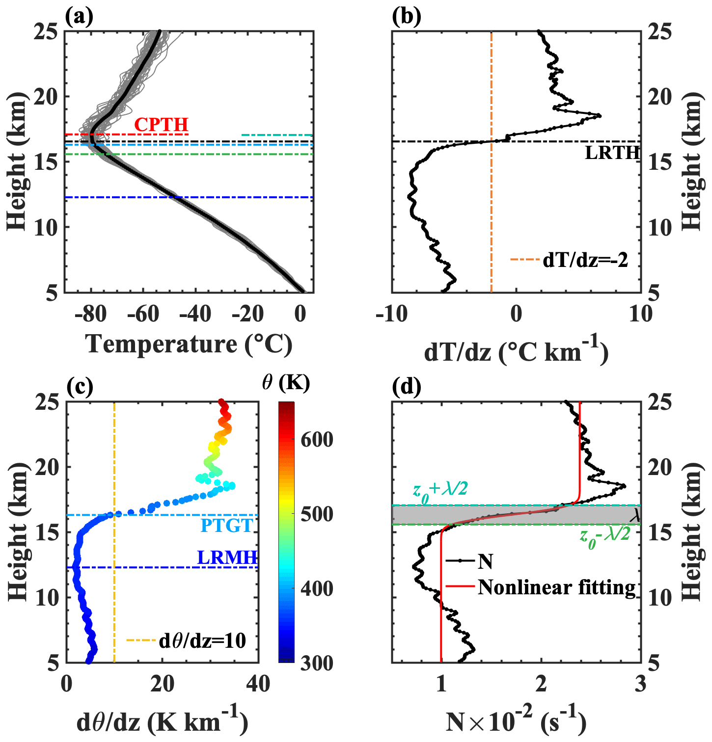
Figure 2 Five different thermal definitions are shown. A 15-point running mean was adopted for temperature and potential-temperature profiles. (a) Comparisons of the heights of the thermal tropopause detected using different definitions. The temperature profiles (gray lines) were sourced from a tropical site (16.83° N, 112.33° E) in July 2014, and the dashed–dotted black line denotes the average temperature profile of 57 gray profiles (CPTH: CPT height). (b) The temperature lapse rate profile and LRT (LRTH: LRT height). (c) The potential-temperature lapse rate profile, LRM, and PTGT (LRMH: LRM height). (d) Curve fit to N².

2.2.1 The cold-point tropopause and potential-temperature lapse rate minimum (LRM) tropopause

The atmospheric stability within the tropical tropopause layer is affected by convection in the troposphere and radiation in the stratosphere (Gettelman and Forster, 2002b; Thuburn and Craig, 2002). The CPT is the coldest point in the temperature profile and marks a sharp increase in stability, above which the potential-temperature profile is close to radiative equilibrium (Gettelman and Forster, 2002a; Randel and Park, 2019; Pan et al., 2014, 2018). The CPT height (CPTH; Fig. 2a) and LRM height (LRMH; Fig. 2c) are also adopted to characterize the upper and lower boundaries of the tropical tropopause layer (Gettelman and Forster, 2002b; Alappattu and Kunhikrishnan, 2010; Seidel et al., 2001). The CPTH almost coincides with the minimum saturated-water-vapor mixing ratio (Fueglistaler et al., 2009; Kley et al., 1979; Randel and Park, 2019), and stratospheric water vapor concentration is mainly determined by the tropopause temperature (Rosenlof and Reid, 2008; Rosenlof, 2003; Xie et al., 2020). Furthermore, LRMH has three physical meanings (Gettelman and Forster, 2002b; Ravindrababu et al., 2020):

1. It refers to the maximum height at which convection still affects temperature in the upper troposphere.

2. It pertains to the height at which temperature begins to be constrained by stratospheric radiation.

3. It coincides with the height corresponding to the minimum ozone mixing ratio.

2.2.2 Lapse rate tropopause

The LRT, defined by the WMO, is widely utilized (Liu et al., 2019; Randel et al., 2007a; Rieckh et al., 2014; Schmidt et al., 2004, 2006; Xian and Homeyer, 2019; Hoffmann and Spang, 2022; Feng et al., 2012). The LRT definition is as follows:

• i.

  The first tropopause is defined as the lowest level at which the lapse rate decreases to 2 °C km⁻¹ or less, provided that the average lapse rate between this level and all higher levels within 2 km does not exceed 2 °C km⁻¹.

• ii.

  Above the first tropopause, if the average lapse rate between any level and all higher levels within 1 km exceeds 3 °C km⁻¹, then a second tropopause is defined using the same criterion as in the first point. This tropopause may be either within or above the 1 km layer.

The LRT is generally considered to be the most reliable definition due to its nearly universal applicability and its ability to identify the approximate locations of the sharpest gradients of stability and chemical composition in the UTLS (Gettelman et al., 2011; Pan et al., 2018; Hoffmann and Spang, 2022). The WMO method described in the appendix of Maddox and Mullendore (2018) was adopted to calculate the average lapse rate.

2.2.3 Curve fit to Brunt–Väisälä frequency

Buoyancy frequency (N; units in s⁻¹) is an indicator of atmospheric static stability, which is characterized by the vertical potential-temperature lapse rate (Homeyer et al., 2010; Birner, 2006; Gettelman and Wang, 2015; Bai et al., 2017) and is expressed as follows:

$$\begin{array}{}\text{(1)}& N^{\mathrm{2}}={\displaystyle \frac{g}{\mathit{\theta }}}{\displaystyle \frac{\partial \mathit{\theta }}{\partial z}},\end{array}$$

where g is the gravitational constant, θ is the potential temperature, and z is the altitude. A primary characteristic of the tropopause layer is the drastic change in static stability when crossing it. According to the discrete jump in N, N is fitted using a nonlinear least-squares method (Fig. 2d), as proposed by Homeyer et al. (2010), to detect tropopause structures. This is expressed as follows:

$$\begin{array}{}\text{(2)}& N\left(z\right)=N_{\mathrm{trop}}+{\displaystyle \frac{N_{\mathrm{strat}}-N_{\mathrm{trop}}}{\mathrm{2}}}\left[\mathrm{1}+\mathrm{erf}\left({\displaystyle \frac{\mathrm{2}(z-z_{\mathrm{0}})}{\mathit{\lambda }}}\right)\right],\end{array}$$

where N_trop and N_strat are the asymptotic values of N in the troposphere and stratosphere, respectively; z₀ is the midpoint of the tropopause height; λ is the thickness of the transition layer; and erf represents the error function. N_trop, N_strat, z₀, and λ can be obtained using nonlinear least-squares fitting, where N_trop=0.0 s⁻¹, N_strat=25.0 s⁻¹, and λ=1 km are the initial values of the fitting and z₀ is calculated according to the WMO definition. In order to reduce the fitting error, data from altitudes lower than 5 km are discarded. Nonlinear fitting of N can directly yield the upper and lower boundaries of the tropopause layer (Fig. 2d).

2.2.4 Potential-temperature-gradient tropopause

The PTGT (Fig. 2c), a modern stability-based definition of the tropopause developed by Tinney et al. (2022), serves as an alternative to the LRT and provides additional insights into tracer–tracer stratosphere–troposphere exchange. The PTGT uses the vertical gradient of potential temperature as a stability metric to identify the greatest composition change in the tropopause transition layer. Its definition is similar to that of the LRT and is outlined as follows:

• i.

  The first tropopause is defined as the lowest level at which the potential-temperature gradient increases to 10 K km⁻¹, provided that the potential-temperature gradient between this level and all higher levels within 2 km does not fall below 10 K km⁻¹.

• ii.

  Above the first tropopause, if the potential-temperature gradient between any level and all higher levels within 1 km falls below 10 K km⁻¹, then a second tropopause may be defined in the same manner as the first tropopause, although a potential-temperature-gradient threshold of 15 K km⁻¹ is used.

2.3 New bi-Gaussian method

It can be seen in Fig. 2 that the tropopause heights identified by the five aforementioned definitions are quite different in some cases (Wirth, 2000; Pan et al., 2018; Bian, 2009). Moreover, each definition is not universally applicable, and most definitions provide limited information about the transition layer structures.

The CPT and LRT exhibit good applicability in the tropics, mainly due to the simple terrain and the minimal impact of weather system intrusions. However, the limitations of these two definitions become apparent in the extratropics, as shown in Fig. 3a. The blue crossline represents the measured temperature profile, and the dotted red line represents the temperature lapse rate. According to the WMO algorithm, points C and D represent the first and second LRT heights (LRTH1 and LRTH2), respectively. Point B (CPTH) is quantitatively comparable with point D (LRTH2); however, the CPT fails to identify point A, which corresponds to LRTH1 (point C). Therefore, the CPT is unable to characterize the double-tropopause (DT) structure.

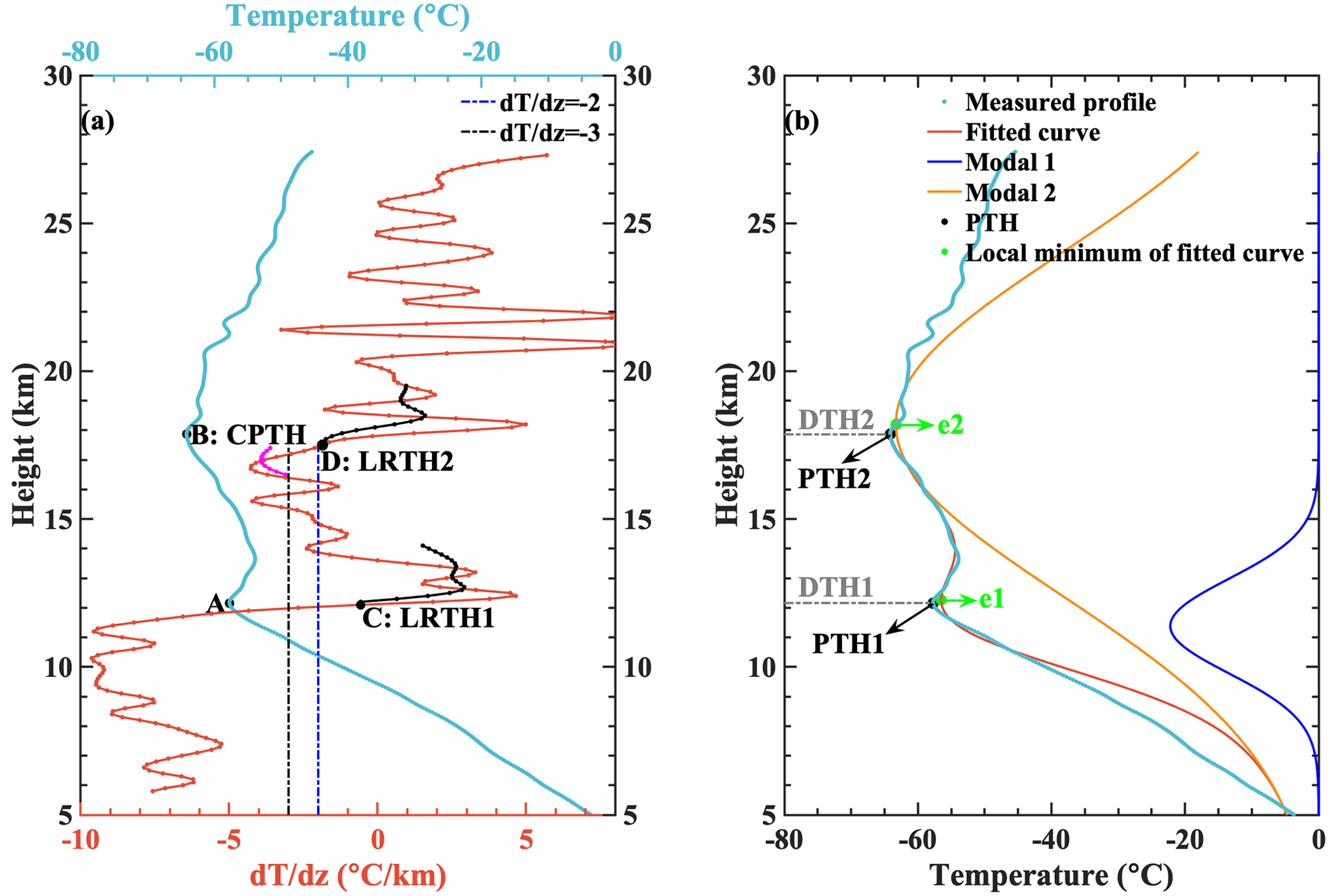
Figure 3 (a) Schematic diagram illustrating the limitations of the CPT. The temperature profile was sourced from a site (38.37° N, 106.2° E) at 12:20 (local time) on 17 June 2014. Points C and D are defined by the LRT. The dotted black line indicates the average lapse rate between this level and all higher levels within 2 km, and the dotted magenta line indicates the average lapse rate between any level and all higher levels within 1 km. (b) An example of bi-Gaussian function fitting used to detect the tropopause heights. Above 15 km, mode 1 equals zero, and mode 2 perfectly coincides with the fitted curve.

Inspired by Fig. 3, both point A and point B represent local-temperature-minimum points within a specific height range. Therefore, the local cold point is used to replace the coldest point in this study. The local cold point is defined as follows: assuming that there exists a certain height (h₀; units in kilometers) at which the temperature is the coldest in the interval h₀−1 to h₀+1, we logically define h₀ as the possible tropopause height (PTH; units in kilometers), hereinafter referred to as the “target”. The target-seeking range (TH_min to TH_max; units in kilometers) is confined to minimize the identification error. TH_min and TH_max correspond to the lower and upper limits of the tropopause height, respectively, defined as follows (Liu et al., 2021):

$$\begin{array}{}\text{(3)}& {\displaystyle }{\mathrm{TH}}_{\min }=\mathrm{2.5}\times \left(\mathrm{3}+\cos \left(\mathrm{lat}\times \mathrm{2}\right)\right),\text{(4)}& {\displaystyle }{\mathrm{TH}}_{\max }=\mathrm{2.5}\times \left(\mathrm{7}+\cos \left(\mathrm{lat}\times \mathrm{2}\right)\right),\end{array}$$

where “lat” (units in degrees), which needs to be converted to radians, is the latitude of the observation sites.

There are two reasons for constraining the search range:

1. to avoid unrealistically high or low tropopause heights;

2. to increase computational speed (Reichler et al., 2003; Li et al., 2017).

What cannot be ignored is the presence of triple tropopauses, even though the occurrence frequency of triple tropopauses is very low. The third tropopause is mainly distributed at ∼ 50 hPa (Anel et al., 2007; Xu et al., 2014). Therefore, it is assumed that there are at most double tropopauses within the height interval of TH_min to TH_max. An example can be found in Fig. S3 in the Supplement.

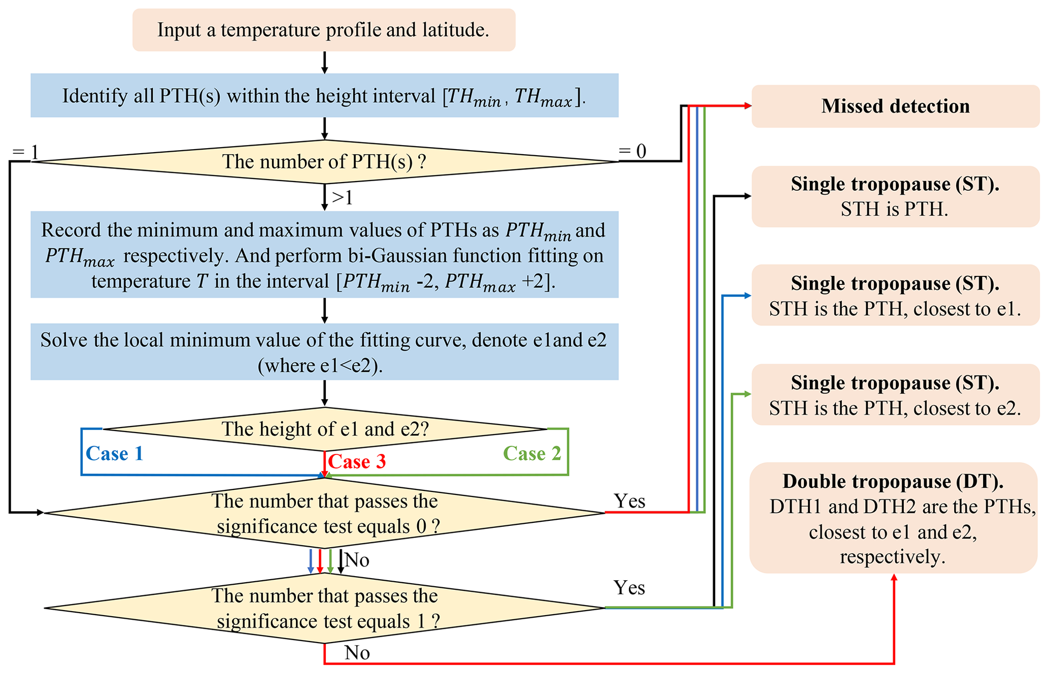
Figure 4 A flow chart illustrating how to use the bi-Gaussian function to fit temperature profiles for the identification of both the tropopause height and the DT structure. The judgment criteria for case 1, case 2, and case 3 are listed in Table 2.

The detailed steps to identify the prominent target(s) are presented in Fig. 4, and the specific steps are delineated below:

1. Target seeking. Identify the PTH(s) within the height interval of TH_min to TH_max. If the number of PTHs is equal to 1, proceed to step 4; otherwise, follow the subsequent steps.

2. Curve fitting. Record the minimum and maximum values of the PTHs as PTH_min and PTH_max, respectively. Bi-Gaussian function fitting is performed on the temperature profiles in a specific height interval (PTH_min−2 to PTH_max+2). The function is expressed as Eq. (5), where $a\mathrm{1}\cdot \exp \left(-{\left(\frac{x-b\mathrm{1}}{c\mathrm{1}}\right)}^{\mathrm{2}}\right)$ and $a\mathrm{2}\cdot \exp \left(-{\left(\frac{x-b\mathrm{2}}{c\mathrm{2}}\right)}^{\mathrm{2}}\right)$ are referred to as mode 1 and mode 2 of the bi-Gaussian function, respectively.

   $$\begin{array}{}\text{(5)}& f\left(x\right)=a\mathrm{1}\cdot \exp \left(-{\left({\displaystyle \frac{x-b\mathrm{1}}{c\mathrm{1}}}\right)}^{\mathrm{2}}\right)+a\mathrm{2}\cdot \exp \left(-{\left({\displaystyle \frac{x-b\mathrm{2}}{c\mathrm{2}}}\right)}^{\mathrm{2}}\right)\end{array}$$

3. Conditional judgment. Solve for the local-temperature-minimum points of the fitted curve, namely e₁ and e₂, and determine whether e₁ and e₂ (units in kilometers) are within the specified interval (PTH_min−2 to PTH_max+2). If the condition is satisfied, the values are considered valid; otherwise, they are deemed invalid.

4. Significance tests. Ensure that the inversion layer strength, which is represented by the slope of the linear fit to the temperature profiles in a certain range (valid PTH(s) to valid PTH(s) + 2), is not less than 0.5 °C km⁻¹ (Randel et al., 2007b). Otherwise, it is invalid.

5. Identification results. Determine the PTH(s) closest to the final valid value(s), which is (are) the tropopause height(s). (In the following, the abbreviation STH specifically refers to the single-tropopause (ST) height, and DTH1 and DTH2 refer to the first and second DT heights, respectively.)

Table 2 Criteria for conditional judgments. The units of PTH_min, PTH_max, e₁, and e₂ are given in kilometers.

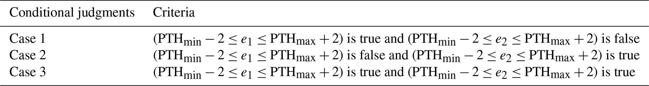
Figure 3b shows an example of using the new method to identify tropopause heights, where PTH1 and PTH2 indicate the first DT height (DTH1) and the second DT height (DTH2), respectively. Table 3 summarizes the results and goodness-of-fit statistics from the bi-Gaussian function fit to the temperature profile, as shown in Fig. 3b.

The coefficient of determination (R²) is used to evaluate the performance of the bi-Gaussian function and is expressed as

$$\begin{array}{}\text{(6)}& R^{\mathrm{2}}=\mathrm{1}-{\displaystyle \frac{\mathrm{SSE}}{\mathrm{SST}}},\end{array}$$

where the sum of the squares due to error corresponds to $\mathrm{SSE}={\sum }_{i=\mathrm{1}}^n(X_i-Y_i{)}^{\mathrm{2}}$ and the total sum of the squares corresponds to $\mathrm{SST}={\sum }_{i=\mathrm{1}}^n{\left(Y_i-\stackrel{\mathrm{‾}}{Y}\right)}^{\mathrm{2}}$. Here, X_i (units in °C) and Y_i (units in °C) are the fitting and measurement temperature profiles, respectively; $\stackrel{\mathrm{‾}}{Y}$ is the mean of Y_i; and n is the number of samples.

Table 3 The results and goodness-of-fit statistics for the bi-Gaussian function fitting to the temperature profile shown in Fig. 3b.

3 Feasibility analysis of the bi-Gaussian method

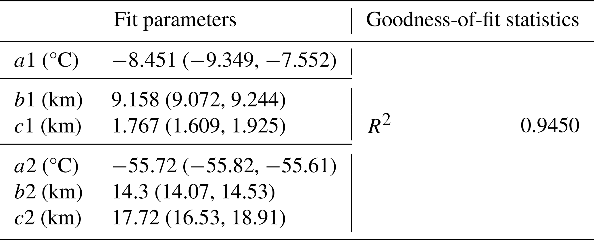
In 2014, 78 758 temperature profiles were employed to discuss the feasibility of the bi-Gaussian method, including the ability of the bi-Gaussian function to effectively interpret temperature profiles, and to compare it with existing definitions.

Figure 5 Goodness-of-fit statistics (with respect to the coefficient of determination (R²)) for the bi-Gaussian function fitting to temperature profiles and the cumulative probability distribution.

3.1 Explanation capability of the bi-Gaussian function for UTLS temperature profiles

Of the 78 758 temperature profiles, 68 896 contain no less than one PTH. Figure 5 shows the coefficient of determination (R²), one of the fitting evaluation indexes, for the 68 896 temperature profiles fitted by the bi-Gaussian function. Higher R² values indicate better goodness of fit for the regression model. R² is greater than 0.8 in at least 90 % of temperature profiles, and the average R² value in all profiles reaches 0.9. Consequently, the bi-Gaussian function exhibits excellent potential for accurately explicating temperature profiles in the UTLS, ensuring that PTHs are successfully identified.

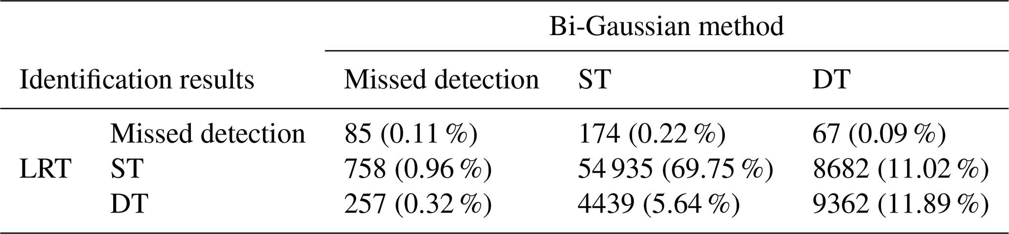
Table 4 Identification results of the bi-Gaussian method and the LRT. It is noted that the search range is also limited for the LRT. The percentages represent the proportion of temperature profiles in each case. “Missed detection” indicates that there are no values satisfying the definitions within the search range.

3.2 Comparisons of identification results between the bi-Gaussian method and the LRT

The tropopause structures of 78 758 profiles, identified using two methods, are summarized in Table 4. Limiting the search range can lead to missed detections (Li et al., 2017), as exemplified in Fig. S1 in the Supplement. However, if the search range is expanded, both methods can yield effective identification results. A total of 77 417 profiles have been successfully identified. In total, the DT detection rates for the bi-Gaussian method and the LRT are 23 % and 17.85 %, respectively.

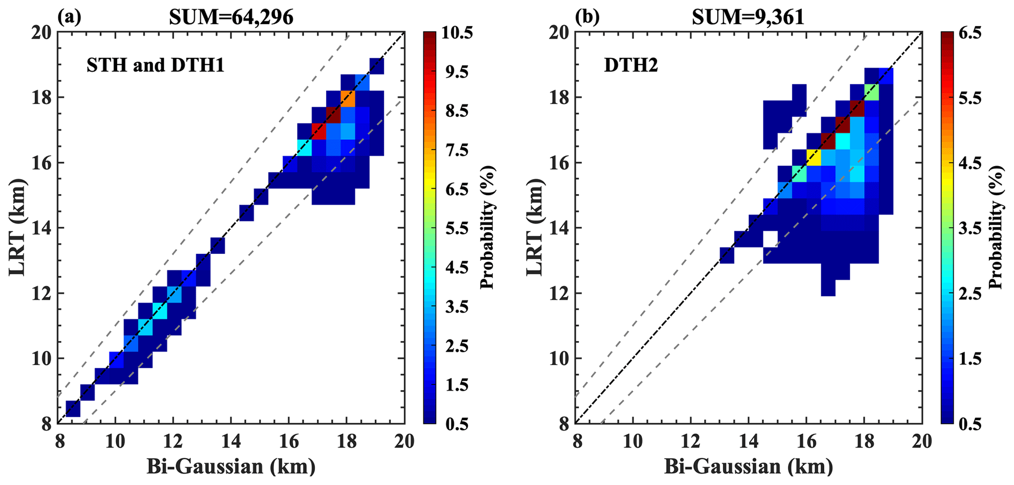
Figure 6 Comparison of identification results between the new bi-Gaussian method and the LRT. The color map represents the number of points, and the dashed gray lines indicate the 10 % error threshold. Panel (a) corresponds to STH and DTH1, while panel (b) corresponds to DTH2.

Figure 6 shows a comparison between the identification results obtained through the new bi-Gaussian method and those obtained via the LRT. Both methods can identify 81.75 % of cases with the same structural types. Specifically, the correlation coefficient (root mean square error) of the two methods with respect to the STH and DTH1 is 0.93 (1.21 km) (Fig. 6a), and at least 95 % of profiles exhibit an error of no more than 10 % between the two methods. There is a discontinuity at 14 km, which is called the “tropopause break”. Although the second DT height identified by the two methods is characterized by a more dispersed distribution (Fig. 6b), 66.67 % of profiles exhibit a percentage difference of no more than 10 %, with the majority of the distribution located on the line y=x, and the root mean square error is 1.7 km. Further, DTH2 identified by the bi-Gaussian method is generally higher than LRTH2 in 3120 profiles.

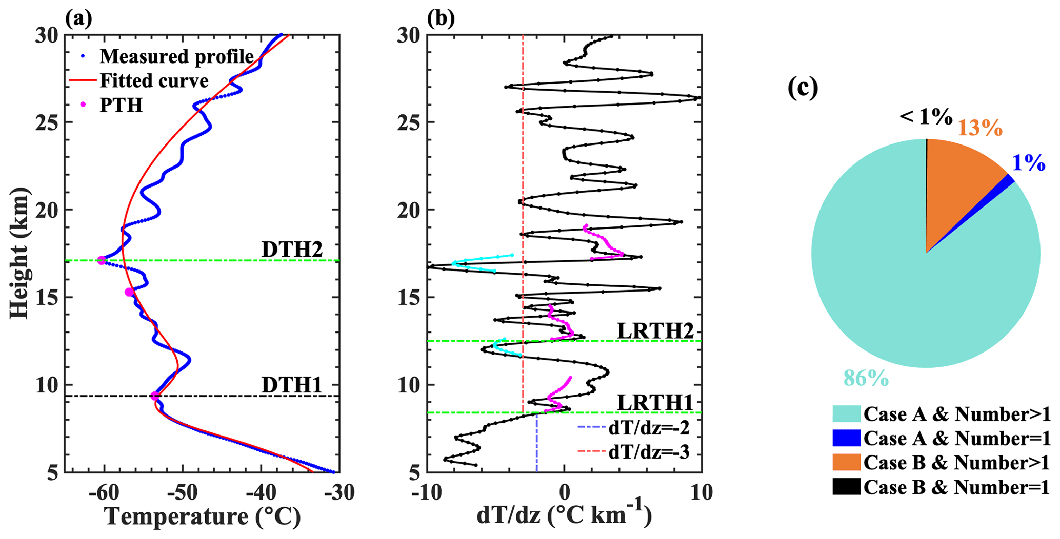
Figure 7 The characteristics of the 3120 temperature profiles, which exhibit a difference of more than 10 % in the second DT height when comparing the bi-Gaussian method with the LRT. (a) A typical profile illustrating the possible reasons for the difference. The temperature profile was sourced from the site (46.6° N, 121.22° E) at 07:20 (local time) on 13 November 2014. (b) The temperature lapse rate profile and LRTH. The dotted magenta line indicates the average lapse rate between this level and all higher levels within 2 km, and the dotted cyan line indicates the average lapse rate between any level and all higher levels within 1 km. (c) Based on the number of inversion layers above the first tropopause and whether there is a higher and colder PTH, the 3120 profiles are classified into four distinct clusters. These clusters are defined for the purpose of gathering characteristic statistical information. (Case A indicates the presence of a higher and colder PTH, while case B is the converse of case A).

Figure 7 shows a characteristic statistical analysis of the 3120 temperature profiles that exhibit significantly different second DT heights between the bi-Gaussian method and the LRT (with a percentage difference of more than 10 %). A typical temperature profile (Fig. 7a) is provided to illustrate the possible reasons for the discrepancy in the second DT height between the two methods. This typical profile displays two obvious characteristics. Firstly, two inversion layers are formed above the first tropopause, indicating that there may be at least one point that fits the criteria for the second tropopause height defined by the LRT. Consequently, LRTH2 may be ambiguous due to the existence of multiple inversion layers (Hoerling et al., 1991). Secondly, it is evident that there is at least one colder PTH above the first tropopause, frequently accompanied by a more significant temperature inversion layer. Notably, the temperatures of two PTHs (magenta dots) are lower than the first tropopause temperature. Out of the 3120 profiles, more than 99 % possess at least one of the features (Fig. 7c), and 86 % possess both features simultaneously. Among these profiles, about 99 % exhibit multiple inversion layers above the first tropopause.

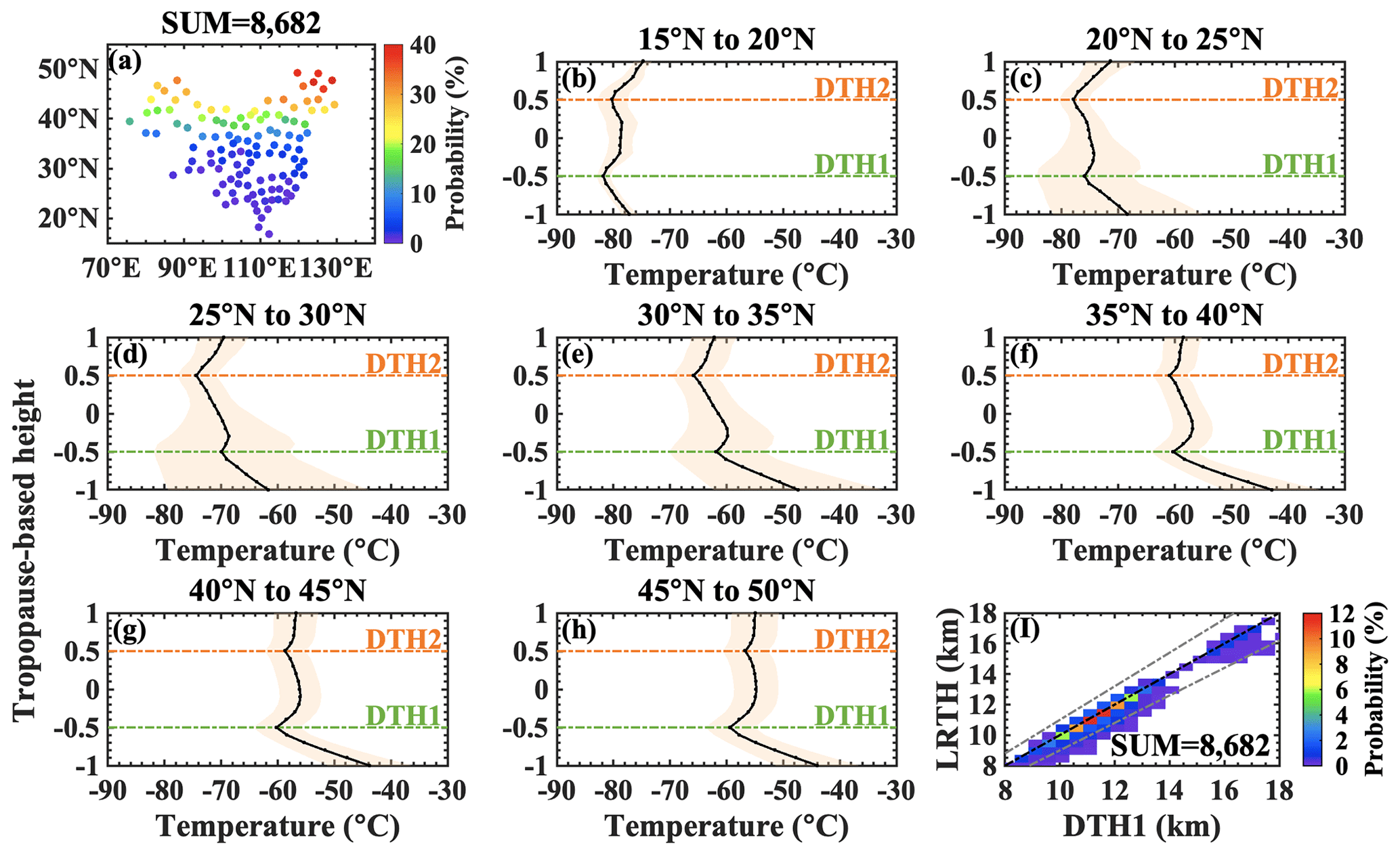
Figure 8 The cases identified by the bi-Gaussian method as corresponding to the DT but identified by the LRT as only corresponding to the ST. (a) Ratio distribution (the ratio of contradictory results to all observations of the site) for the 8682 temperature profiles. (b)–(h) Annual average temperature profiles shown across 5° latitude bands. A tropopause-based height is adopted using the midpoint of DTH1 and DTH2, i.e., (DTH1 + DTH2) $/$ 2, as a reference level. The y axis represents the normalized dimensionless height; i.e., −0.5 and 0.5 represent DTH1 and DTH2, respectively, and 0 represents the midpoint. (i) A comparison of DTH1 between the bi-Gaussian method and LRTH for the 8682 profiles.

There are 14 377 temperature profiles with contradictory results from the LRT and the bi-Gaussian method, of which the largest proportion (8682 profiles) is identified by the bi-Gaussian method as corresponding to the DT but identified by the LRT as only corresponding to the ST. Figure 8 shows the distribution of sites for the 8682 temperature profiles and the annual average temperature profiles with normalized height in each latitude zone. Using the midpoint of DTH1 and DTH2, i.e., (DTH1 + DTH2) $/$ 2, as a reference level, the tropopause-based annual average temperature profiles for each latitude zone (using intervals of 5°) are calculated, as shown in Fig. 8b–h. It is clearly noticeable that there is an inversion layer at both DTH1 and DTH2, and the strength of the inversion layer at DTH2 is significantly weaker than that at DTH1. Additionally, the bimodality is more pronounced at middle and high latitudes. The LRT often fails to capture the weak stability transition (Tinney et al., 2022). The temperature lapse rate between DTH1 and DTH2 is mainly distributed in the range of −1.26 °C km⁻¹ to −2.54 °C km⁻¹, failing to satisfy the condition that the average lapse rate between any level and all higher levels within 1 km exceeds 3 °C km⁻¹. Therefore, the LRT definition of the second tropopause is not satisfied, and these cases are defined as corresponding to the ST. As can be seen in Fig. 8i, LRTH is significantly consistent with DTH1, indicating that the LRT can accurately identify the first tropopause, although it fails to identify the second tropopause. Admittedly, the threshold of 0.5 °C km⁻¹ in the significance tests might account for this contradiction. Below, we describe the reasons for choosing 0.5 °C km⁻¹ as the threshold.

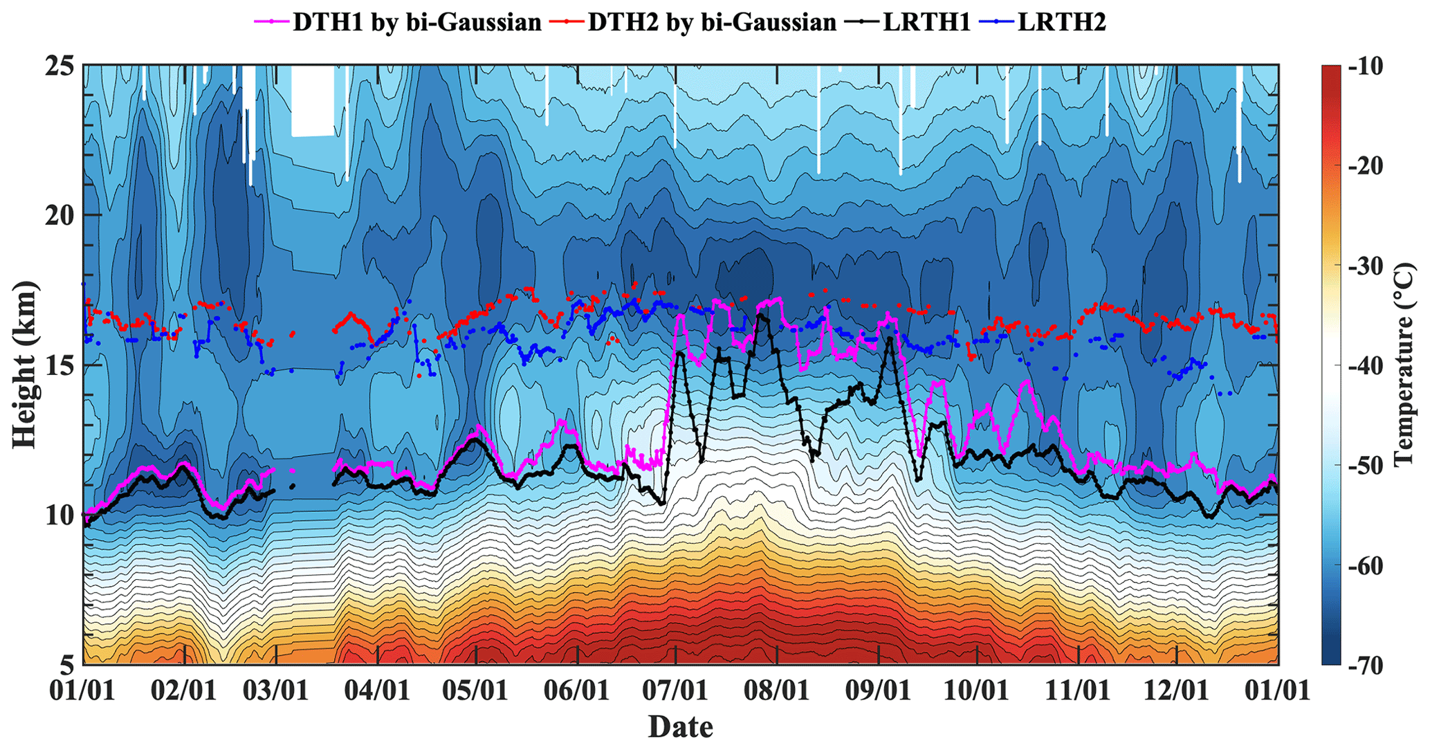
Figure 9 Height–time cross section of temperature profiles (shaded regions) obtained in 2014 from radiosondes at the Kuqa site (49.25° N, 119.7° E). DTH1 (dotted magenta line) and DTH2 (dotted red line) represent the first and second tropopause heights defined by the bi-Gaussian method, respectively. LRTH1 (dotted black line) and LRTH2 (dotted blue line) represent the first and second tropopause heights defined by the LRT, respectively.

The evolution of the temperature field at the Kuqa site (49.25° N, 119.7° E) in 2014 is shown in Fig. 9. There are obviously two local-temperature-minimum layers from January to May along the vertical direction, and the DT structure occurs frequently. With the increase in surface temperature, the lower local-temperature-minimum layer is elevated from June to September, exhibiting a prevailing ST structure. After October, it re-evolves into two local-temperature-minimum layers, prompting the formation of DT structures. The DT structures identified by the bi-Gaussian method are mainly concentrated in winter and spring, while the LRT identified a large proportion of DT structures from May to September. Therefore, the identification results of the bi-Gaussian method are more reasonable and more consistent with the evolution process of atmospheric thermal stratifications. In addition, the upper local-temperature minima observed in November and December are too weak to be detected by the LRT.

The bi-Gaussian function has a good ability to express the temperature profiles pertaining to the UTLS and is able to more stably and obviously identify the spatial and temporal distribution characteristics of the thermal tropopauses. If a higher threshold is set, some DT structures become difficult to identify, as is the case with the LRT. As shown in Fig. 9, the threshold of 0.5 °C km⁻¹ ensures that the bi-Gaussian approach has a good ability to identify weak inversion layers. Figure 9 also reflects the differences in the recognition results of the two methods (as listed in Table 4). The LRT identified more DT structures in summer than the bi-Gaussian method, while the opposite was true in winter.

Similarly, there are 4439 temperature profiles identified by the LRT and the new method as corresponding to the DT and the ST, respectively. However, there is a single PTH in the bi-Gaussian function fitting curve within the range of TH_min to TH_max, indicating a more significant inversion layer. An example can be found in Fig. S4 in the Supplement.

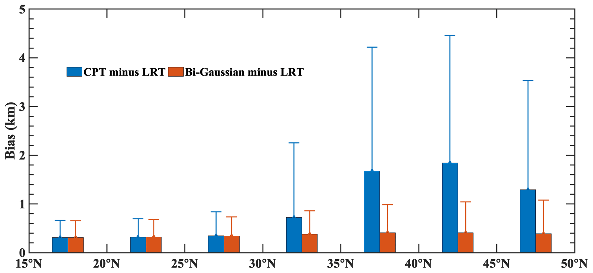
Figure 10 The biases of the bi-Gaussian method and the CPT compared to the LRT at different latitudes.

3.3 Improvement of the bi-Gaussian method over the CPT

The CPTH and LRTH are inconsistent, with a positive bias of about 300–2000 m (Pan et al., 2018; Xia et al., 2021; Schmidt et al., 2004). On the one hand, this difference is caused by the inherent properties of the two definitions (see Fig. S5 in the Supplement) because CPTH represents the transition point at which the temperature lapse rate changes from negative to positive, which is common in the tropics. On the other hand, the CPT defines the highest and coldest inversion layers (if multiple exist) as the tropopause, meaning the two methods cannot identify the same temperature inversion layer (see Fig. 3a). This situation mostly occurs at middle and high latitudes, which may be one of the reasons for the large bias between the CPT and LRT at these latitudes.

The CPT definition is more applicable to the tropics due to the simpler vertical thermal structure in this region, with fewer inversions. The CPT can only return one identification result for both single and multiple structures, which is exactly why the CPT cannot identify multiple structures. Therefore, in the new bi-Gaussian method, we define the local cold point(s) (rather than the CPT) as the possible tropopause height(s), and only the local cold point(s) that has (have) passed the significance test is (are) considered to be the tropopause height(s).

Compared with the CPT, the bi-Gaussian method improves agreement with the LRT. Specifically, the bi-Gaussian method can identify not only the DT structures but also the same temperature inversion layers as the LRT. The identification results from the bi-Gaussian method show less bias compared to the results from the LRT, as shown in Fig. 10. The bias between the CPT and LRT is distributed between 0.31–1.84 km, while the bias between the bi-Gaussian method and the LRT remains stable at 0.37 km, even at mid-latitudes.

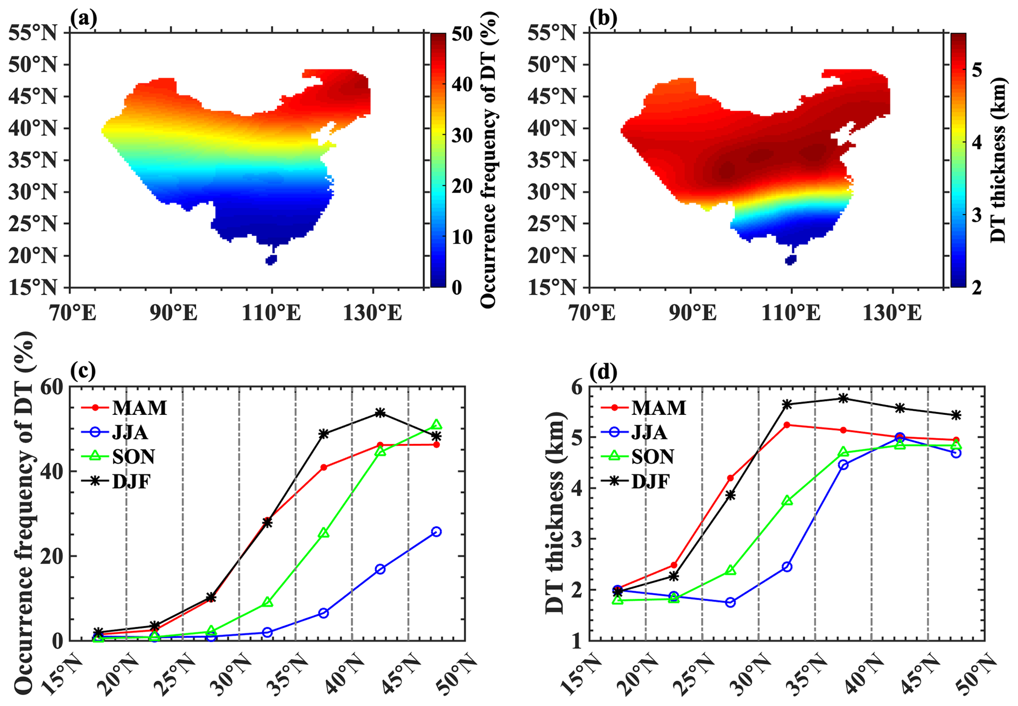
Figure 11 The meridional distribution of the annual (a, b) and seasonal (c, d) mean occurrence frequency (a, c) and thickness (b, d) of the DT in China during 2012–2016. Zonal means were determined for 5° latitude bins.

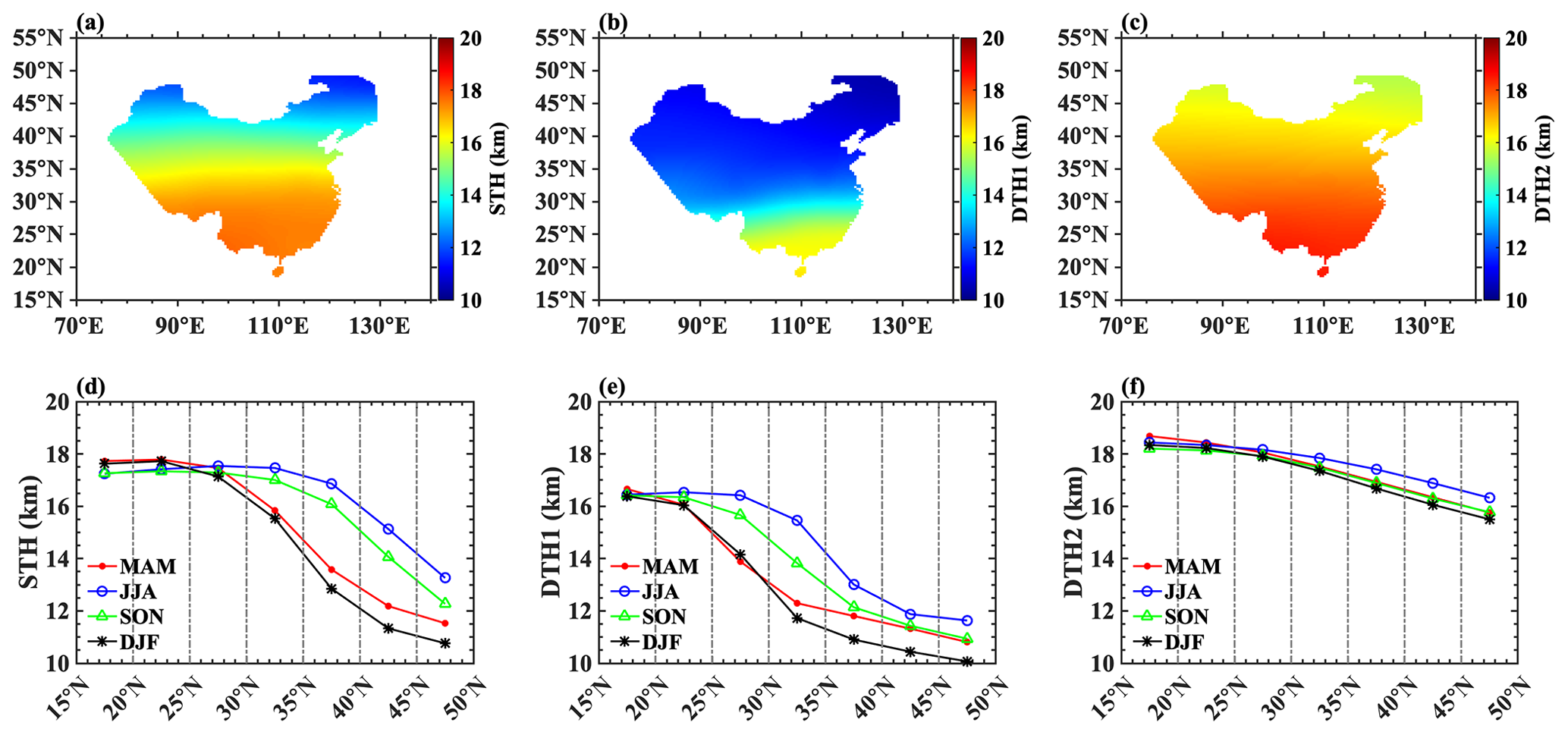
Figure 12 Meridional distributions of the annual and seasonal mean tropopause heights in China during 2012–2016. The first row corresponds to the annual mean STH (a), DTH1 (b), and DTH2 (c). The second row represents the seasonal STH (d), DTH1 (e), and DTH2 (f) for spring, summer, fall, and winter, respectively.

4 Spatiotemporal characteristics of tropopause structures in China

4.1 Double-tropopause structures: occurrence frequency and thickness

In general, the occurrence frequency of the DT, as shown in Fig. 11a (with thickness shown in Fig. 11b), reaches its maximum in northern China and gradually decreases toward the tropics, showing typical meridional distribution characteristics (Schmidt et al., 2006; Seidel and Randel, 2006; Johnston and Xie, 2020). The maximum annual mean occurrence frequency (thickness) is about 47.19 % (5.42 km), and the minimum is about 1.07 % (1.96 km) in the latitude range of 16–50° N. Additionally, the annual mean occurrence frequency in the latitude range of 30–45° N is about 28.93 %, which is roughly 7.51 times the occurrence frequency in the latitude range of 20–30° N (3.85 %). The phenomenon of DT occurrences being frequent at mid-latitudes has also been recorded in previous studies, which attribute this pattern to the influence of the subtropical jet (STJ) system, whose mean climatological distribution position is about 30–45° N (Schmidt et al., 2006; Seidel and Randel, 2006).

Figure 11c shows the zonal mean of the DT occurrence frequency, determined using 5° latitude bins, with respect to spring (March–April–May; MAM), summer (June–July–August; JJA), fall (September–October–November; SON), and winter (December–January–February; DJF). Taking 30° N as the dividing line, the DT occurrence frequency increases sharply from low to middle latitudes, particularly in winter and spring. The DT occurrence frequency is low (< 10 %) and exhibits no significant seasonal variations at low latitudes. However, it shows obvious seasonal differences at middle latitudes, reaching its largest (∼ 27.82 %–53.71 %) and smallest (∼ 1.89 %–25.65 %) values in winter and summer, respectively. The mean climatological location of the STJ gradually moves southward from 40–45° N in summer to 30–35° N in winter (Chen, 2011) and concurrently becomes stronger. Consequently, a large meridional gradient of DT occurrence frequency usually occurs in the climatological location of the STJ and its adjacent latitude zones (± 5°). The DT occurrence frequency in the latitude range of 45–50° N does not maintain an increasing trend in winter; instead, it shows a downward trend, which is consistent with the results in Randel et al. (2007a) and Schmidt et al. (2006). However, such downward trends are not observed during other seasons.

In Fig. 11b and d, the annual and seasonal mean DT thicknesses are consistent with previous studies (Schmidt et al., 2006), peaking in the latitude region of 30–50° N. The atmospheric temperature in the UTLS over northern China, especially at middle–high latitudes, is primarily affected by cold air intrusion caused by weather systems, such as the Siberian High, the polar vortex, and the Asian winter monsoon (He and Wang, 2016; Woo et al., 2015; Shangguan et al., 2019). Strengthened northern winds are conducive to the advection and subsidence of cold air into eastern Asia, resulting in the convergence of hot and cold currents in the upper troposphere, which is beneficial for the formation of significant temperature inversion layers.

4.2 Tropopause heights

As shown in Fig. 12, STH, DTH1, and DTH2 also manifested a significant meridional structure, similar to LRTH (Schmidt et al., 2004) and CPTH (Tang et al., 2017). STH (DTH1 and DTH2) gradually decreased from 17.74 km (16.55 and 18.50 km) to 11.43 km (10.43 and 15.51 km) in the latitude range of 16–50° N, with DTH2 displaying weaker meridional variation. The meridional distribution of tropopause height from tropical to subtropical regions is discontinuous, a phenomenon known as the “tropopause break”, corresponding to the zone with a high DT occurrence frequency (Randel et al., 2007a; Rieckh et al., 2014; Schmidt et al., 2004; Feng et al., 2012; Xian and Homeyer, 2019; Pan et al., 2004).

The meridional gradients of STH, DTH1, and DTH2 in the latitude range of 30–40° N are significantly larger (Fig. 12d–f), corresponding to the climatological locations of the STJ and the Tibetan Plateau. The tropopause structures at mid-latitudes are asymmetrical in both hemispheres (Xu et al., 2014), with greater complexity observed in the Northern Hemisphere (Xia et al., 2021; Han et al., 2011). In the Northern Hemisphere, the meridional gradient of the first tropopause height is steeper (shallower) in summer (winter) (Randel et al., 2007a), and the DT occurs more frequently (Johnston and Xie, 2020; Schmidt et al., 2006; Zeng et al., 2017) than in the Southern Hemisphere. The Tibetan Plateau, a source of gravity waves (Hoffmann et al., 2013; Khan et al., 2016), may be one of the contributors to the asymmetry between the Northern and Southern hemispheres. During winter, the subtropical westerly jet is located on the southern margin of the Tibetan Plateau (Chen et al., 2006), and atmospheric fluctuations triggered by topography, jet streams, or convection (De La Torre et al., 2004) manifest as strong variations in static stability (Koch et al., 2005), increasing the probability of forming an inversion layer at a lower height. In summer, a strong Asian summer monsoon anticyclone prevails due to the thermal difference between sea and land (Xu et al., 2019; Park et al., 2009; Bian et al., 2020; Liu et al., 2017; Wu et al., 2016; Ma et al., 2023), which can destabilize atmospheric temperature stratification in the UTLS by triggering deep convection and monsoon circulations (Randel and Park, 2006). However, the contributions of the unique thermal and dynamic effects of the Tibetan Plateau across different seasons to the tropopause structures in local and surrounding regions require further study.

5 Conclusions

This study presents a reliable and highly universal method for identifying tropopause structures, based on the concept of local cold points. Temperature profiles are fitted with the bi-Gaussian function to find one (or two) of the most significant local cold points, which is (are) regarded as the tropopause height(s). The bi-Gaussian function demonstrates strong explanatory potential for UTLS temperature profiles, ensuring it can reliably and stably capture the evolution of the tropopause, even in the presence of weak inversion layers. This method will benefit future STE studies and serves as an alternative to previous thermal definitions. In addition, statistical analyses based on the bi-Gaussian method will be conducted in future research to further understand tracer–tracer stratosphere–troposphere exchange, especially regarding DT structures.

Moreover, 5 years of radiosonde data from China (from 2012 to 2016) showed that tropopause structures – specifically, the occurrence frequency and thickness of the DT, STH, DTH1, and DTH2 – display significant meridional distribution characteristics. In the latitude range of 15–50° N, STH (DTH1 and DTH2) gradually decreased from 17.74 km (16.55 and 18.50 km) to 11.43 km (10.43 and 15.51 km), and the DT occurrence frequency (thickness) increased from 1.07 % (1.96 km) to 47.19 % (5.42 km), with a steep variation observed at middle latitudes. Subtropical regions (15–25° N) exhibit ST-dominated conditions throughout the year, while middle–high latitudes (25–35° N) experience a high frequency of DT occurrence, particularly in winter, when the occurrence frequency exceeds 50 %. This may be related to STJ activities and the intrusion of cold air from the north, caused by weather systems in winter. Notably, the climatic location of the STJ and its adjacent latitude zones (± 5°) exhibit a sharp increase in occurrence frequency. Furthermore, the DT thickness at middle–high latitudes during winter is no less than 5 km. Moreover, tropopause structures over the Tibetan Plateau differ from those in the same latitudinal zone, likely due to unique atmospheric circulation structures, such as the Asian summer monsoon anticyclone, planetary wave breaking, orographic gravity waves, and atmospheric temperature disturbances in the UTLS. However, the underlying mechanisms require further investigation.