the Creative Commons Attribution 4.0 License.
the Creative Commons Attribution 4.0 License.
 | 04 Sep 2023
Investigation of meteorological conditions and BrO during ozone depletion events in Ny-Ålesund between 2010 and 2021
Bianca Zilker
Andreas Richter
Anne-Marlene Blechschmidt
Peter von der Gathen
Ilias Bougoudis
Tim Bösch
John Philip Burrows
During polar spring, ozone depletion events (ODEs) are often observed in combination with bromine explosion events (BEEs) in Ny-Ålesund. In this study, two long-term ozone data sets (2010–2021) from ozonesonde launches and in situ ozone measurements have been evaluated between March and May of each year to study ODEs in Ny-Ålesund. Ozone concentrations below 15 ppb were marked as ODEs. We applied a composite analysis to evaluate tropospheric BrO retrieved from satellite data and the prevailing meteorological conditions during these events. During ODEs, both data sets show a blocking situation with a low-pressure anomaly over the Barents Sea and anomalously high pressure in the Icelandic Low area, leading to transport of cold polar air from the north to Ny-Ålesund with negative temperature and positive BrO anomalies found around Svalbard. In addition, a higher wind speed and a higher, less stable boundary layer are noticed, supporting the assumption that ODEs often occur in combination with polar cyclones. Applying a 20 ppb ozone threshold value to tag ODEs resulted in only a slight attenuation of the BrO and meteorological anomalies compared to the 15 ppb threshold. Monthly analysis showed that BrO and meteorological anomalies are weakening from March to May. Therefore, ODEs associated with low-pressure systems, high wind speeds, and blowing snow more likely occur in early spring, while ODEs associated with low wind speed and stable boundary layer meteorological conditions seem to occur more often in late spring. Annual evaluations showed similar weather patterns for several years, matching the overall result of the composite analysis. However, some years show different meteorological patterns deviating from the results of the mean analysis. Finally, an ODE case study from the beginning of April 2020 in Ny-Ålesund is presented, where ozone was depleted for 2 consecutive days in combination with increased BrO values. The meteorological conditions are representative of the results of the composite analysis. A low-pressure system arrived from the northeast to Svalbard, resulting in high wind speeds with blowing snow and transport of cold polar air from the north.
Please read the corrigendum first before continuing.
-
Notice on corrigendum
The requested paper has a corresponding corrigendum published. Please read the corrigendum first before downloading the article.
-
Article
(33659 KB)
-
The requested paper has a corresponding corrigendum published. Please read the corrigendum first before downloading the article.
- Article
(33659 KB) - Full-text XML
- Corrigendum
- BibTeX
- EndNote


During polar spring, large losses of ozone in the lower troposphere are observed regularly. These “ozone depletion events” (ODEs) often occur in combination with enhanced bromine monoxide (BrO) values. In the 1980s, Barrie et al. (1988) first reported a link between the ozone loss and the appearance of reactive bromine, further known as “bromine explosion events” (BEEs) (Barrie and Platt, 1997), and concluded that ozone destruction appears when sunlight is present in autocatalytic chain reactions involving BrOx (Br, BrO) radicals. Usually, these events last between a couple of hours and a few days, where ozone can be depleted below the detection limit of the instruments (e.g. Langendörfer et al., 1999; Jacobi et al., 2006). The current understanding of this ozone depletion is that in a heterogeneous, autocatalytic, chemical chain reaction cycle, molecular bromine (Br2) is released from the cryosphere (e.g. sea ice, brine, snow) into the troposphere (e.g. Simpson et al., 2007). In the presence of sunlight, Br2 is photolysed, creating bromine (Br) radicals (Reaction R1) that react with ozone to yield bromine oxide, BrO (Reaction R2). The resulting BrO can be observed by satellite and ground-based measurements using the differential optical absorption spectroscopy (DOAS) technique (Platt and Stutz, 2008). After the oxidation, BrO reacts with HO2 and forms HOBr (Reaction R3), which is scavenged and enters the cryosphere again, converted from the gas phase into a liquid or solid phase (Reaction R4). In the liquid phase, HOBr reacts with halogens to form Br2 (Reaction R5), which is released to the atmosphere, and the cycle starts over again. For each Br atom scavenged from the gas phase, two Br atoms are released from the liquid phase. Thus, the mechanism is autocatalytic and rapidly accelerating.
There is also a potential catalytic depletion cycle involving bromine chloride (BrCl). However, chlorine (Cl) atoms, unlike Br atoms, react with methane (CH4) and alkyl volatile organic carbon (VOC) compounds in the troposphere, reducing the Cl atoms concentrations available for further reactions in the catalytic cycle.
There are still uncertainties about the sources of the bromide ion Br− (Reaction R5) in the cryosphere and the initial release mechanism of Br2 that leads to the large BrO plumes observed in polar spring. So far, it is known that sea ice and saline surfaces are associated with the Br source. Since first-year sea ice is saltier than multi-year sea ice, it is regarded as a more likely contributor to bromine release (Simpson et al., 2007). Other potential sources include frost flowers (Kaleschke et al., 2004), sea salt aerosols from blowing snow (Yang et al., 2010), sea spray from open leads (Peterson et al., 2015), and BrO transported down from the stratosphere into the troposphere (Salawitch et al., 2010). Furthermore, low temperatures favour the bromine explosion reaction, and a pH below 6.5 seems to be necessary to start the activation of the autocatalytic reaction cycle described above (Fickert et al., 1999). The potential triggering of the acid-catalysed bromine explosion by carbonate precipitation in cold brine and the temperature dependence of Reaction (R5) have also been discussed in Sander et al. (2006). In addition to bromine, iodine also appears to play an important role in ozone depletion in spring and is present all year as long as there is sunlight (Benavent et al., 2022).
Regarding the meteorological conditions leading to ODEs or BEEs, Jones et al. (2009) found two different situations favouring the events: (1) low wind speeds and a stable boundary layer, where bromine can accumulate and deplete ozone, and (2) high wind speeds above approximately 10 m s−1 with blowing snow and a higher, unstable boundary layer. The first condition was observed, for example, during a ship cruise west and northwest of Svalbard in 2003 (Jacobi et al., 2006). Here, the ozone concentration was near or below the instrument's detection limit for more than 5 d, along with elevated BrO concentrations and a stable shallow boundary layer with low wind speeds. Therefore, they concluded that this event was local and that no transport of ozone-depleted air took place. The second condition often occurs in combination with polar cyclones, where bromine can be recycled aloft on snow and aerosol surfaces (Peterson et al., 2017). The photolytic lifetime of BrO is approximately 1 min (e.g. Lehrer et al., 2004; Pratt et al., 2013). Nevertheless, several studies (e.g. Begoin et al., 2010; Blechschmidt et al., 2016; Zhao et al., 2016) showed BrO plumes in combination with polar cyclones that were transported over the Arctic region for several days, leading to the assumption that BrO must have been recycled on blowing snow or aerosol surfaces, increasing the lifetime of the BrO plumes. Due to a good spatial coverage, large BrO plumes are best observed from satellites. The first observations were reported in 1998 using the GOME instrument (Wagner and Platt, 1998; Richter et al., 1998; Chance, 1998). Subsequently, polar tropospheric BrO columns were also retrieved from measurements of the SCIAMACHY instrument (Jacobi et al., 2006), OMI (Salawitch et al., 2010), GOME-2 (Begoin et al., 2010; Theys et al., 2011), and TROPOMI (Seo et al., 2019). Recently, a long-term tropospheric BrO data set (1996 to 2017) was established by Bougoudis et al. (2020) using observations from four different satellites. It shows an increasing trend of tropospheric BrO of around 1.5 % yr−1 during polar springs for the evaluated time period. Seo et al. (2020) investigated the relation between areas of elevated total BrO columns and meteorological parameters in the Arctic and Antarctic sea ice regions using 10 years of GOME-2 measurements. In a statistical analysis, meteorological conditions were compared to a 10-year mean during enhanced BrO periods, and distinct spatial patterns were identified. They found that atmospheric low pressure, with low temperature, high wind speed, and a low tropopause height, prevailed in areas of enhanced BrO. In this study, a similar approach is applied, but instead of examining large-scale regions with elevated BrO, we evaluate time periods of ozone-depleted air at a specific location to identify the prevailing meteorological conditions during ODEs.
This study focuses on ODEs recorded in Ny-Ålesund, Svalbard (Norway), a small town on the shore of the bay of Kongsfjorden. For almost 1 decade, the bay has not been completely frozen in the winter months (Serrat, 2015). Mainly icebergs and patches of ice sheets occur in the otherwise ice-free bay during winter and early spring. Ny-Ålesund is the northernmost permanent civilian research station, and several institutes have installed measurement facilities and instruments at the site, which gives us an opportunity to examine ODEs from several aspects. The first studies of ODEs in combination with increased bromine values in the Ny-Ålesund area were published as part of the ARCTOC (Arctic Tropospheric Ozone Chemistry) campaigns in 1995 and 1996 (e.g. Tuckermann et al., 1997; Langendörfer et al., 1999). Luo et al. (2018) observed enhanced BrO values in combination with depleted ozone in Ny-Ålesund using a ground-based MAX-DOAS instrument. Sea ice, which was transported to Kongsfjorden during that time, was assumed to be the major source of Br2. Chen et al. (2022) recently reported a BEE in Ny-Ålesund that was associated with a polar cyclone approaching Svalbard, leading to high wind speeds and blowing snow. Here, it was assumed that the observed BrO was transported and recycled on its way to Ny-Ålesund.
In this study, the occurrence of ODEs in Ny-Ålesund and their dependence on meteorological conditions is investigated. To this end, ozone data measured between 2010 and 2021 in Ny-Ålesund are combined with satellite BrO observations, sea ice concentrations, and meteorological parameters in a composite analysis. In addition, a case study of a severe ODE observed in Ny-Ålesund preceded by a polar cyclone in the beginning of April 2020 is presented.
The paper is structured as follows: in Sect. 2, all data sets used and the composite analysis are introduced. In Sect. 3, the results of the composite analysis are described and discussed (Sect. 3.1). This is complemented by a sensitivity study in Sect. 3.2, which analyses the influence of different threshold values (Sect. 3.2.1) and investigates whether the results of the composite analysis are only valid in given months (Sect. 3.2.2) or years (Sect. 3.2.3). In Sect. 3.3, a severe ODE case study is discussed. The paper ends with a summary and conclusion (Sect. 4).
2.1 Ozone data
For this study, two ozone data sets have been used to analyse ODEs in Ny-Ålesund. The first data set originates from ozonesondes that have been launched from Ny-Ålesund at least once per week since 1992. The sounding frequency increases up to about two to three times per week plus additional launches during campaigns. Data for ozonesonde records are publicly available from the Network for the Detection of Atmospheric Composition Change (NDACC) at https://www.ndacc.org (last access: 16 February 2022). The vertically resolved ozonesonde profiles allow us to study the altitude distribution of ODEs in the boundary layer with an ozone detection limit of 2 ppb in this area. The majority of ODEs occur in the lower troposphere. Consequently, the ozonesonde data were evaluated from the surface up to 4 km. An examination of the ozonesonde data above 4 km revealed no ozone concentrations below the two applied threshold values of 15 and 20 ppb (see below).
To overcome the irregular temporal coverage of the ozonesonde record and allow for better statistics, additional in situ ozone measurements (detection limit of 1 ppb) from the Zeppelin observatory on top of Zeppelin mountain (474 m) about 1 km south of Ny-Ålesund are included in our analyses. The observatory is located higher above sea level and does not necessarily capture all ODEs at sea level. Ozone concentrations have been monitored there almost continuously at hourly resolution since October 1988 and are provided by the Norwegian Air Research Institute (Platt et al., 2022). This data set enables a much better temporal resolution of ODEs than the ozonesondes, which is helpful for the statistical analysis later, but due to the fixed location no altitude profiles are possible.
Since ODEs occur in polar spring, both data sets are evaluated between March and May for each year from 2010–2021. The data are separated into points in time with ODEs and points in time without ODEs, using an ozone volume mixing ratio threshold value of 15 ppb. Background levels of ozone in the boundary layer are normally around 40 ppb. The sensitivity of the meteorological conditions and BrO to the choice of the threshold value is further discussed in Sect. 3.2. Both data sets are shown in Fig. 1. All ozonesondes that contain ozone values below 15 ppb at altitudes between 0 and 2 km are marked as ODE and displayed in red, the remaining ozonesondes are coloured in blue. For the Zeppelin data, every hour below the threshold value is counted as ODE and displayed in red, and every hour above is shown in blue. We use the name ODE here despite it is not being quite correct in this context, since all consecutive hours below the threshold are individually marked with the abbreviation ODE, which is not consistent with the definition of ODE. However, in order to avoid introducing a new abbreviation, we kept the term ODE when referring to individual hours with ozone values below the threshold.
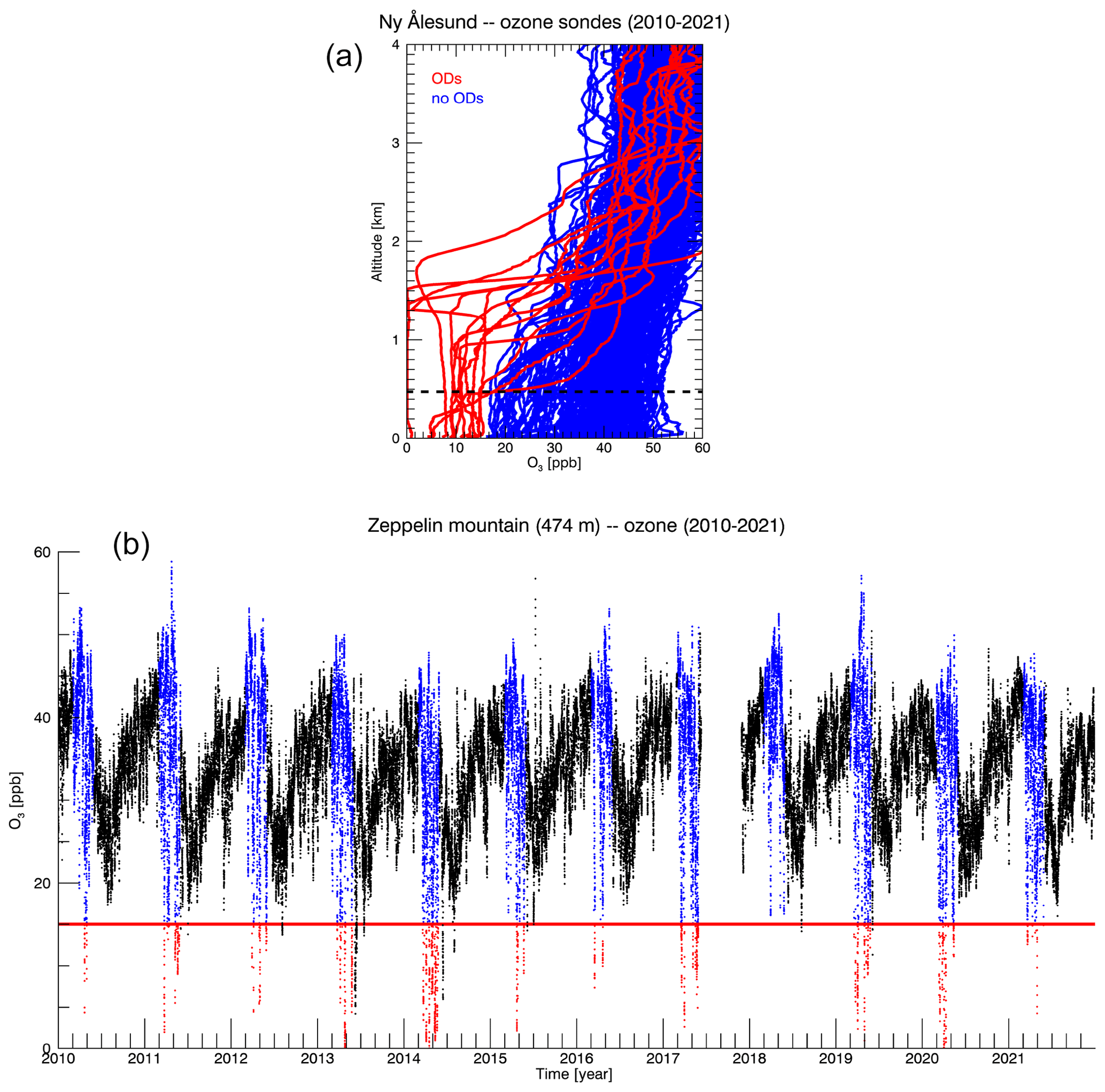
Figure 1(a) All ozone launches between March and May from 2010 to 2021. Every launch with values below 15 ppb between 0 and 2 km is marked in red as ODE, and the other launches are shown in blue. The dashed line indicates the altitude of the Zeppelin observatory. (b) All hourly ozone measurements from Zeppelin observatory from 2010 to 2021. Every hour between March and May with ozone concentration below the red line (15 ppb) is labelled as ODE. All measurements from June to March are in black. Note that the measurements in June below the red line are not included in the ODE data set because this period is not evaluated.
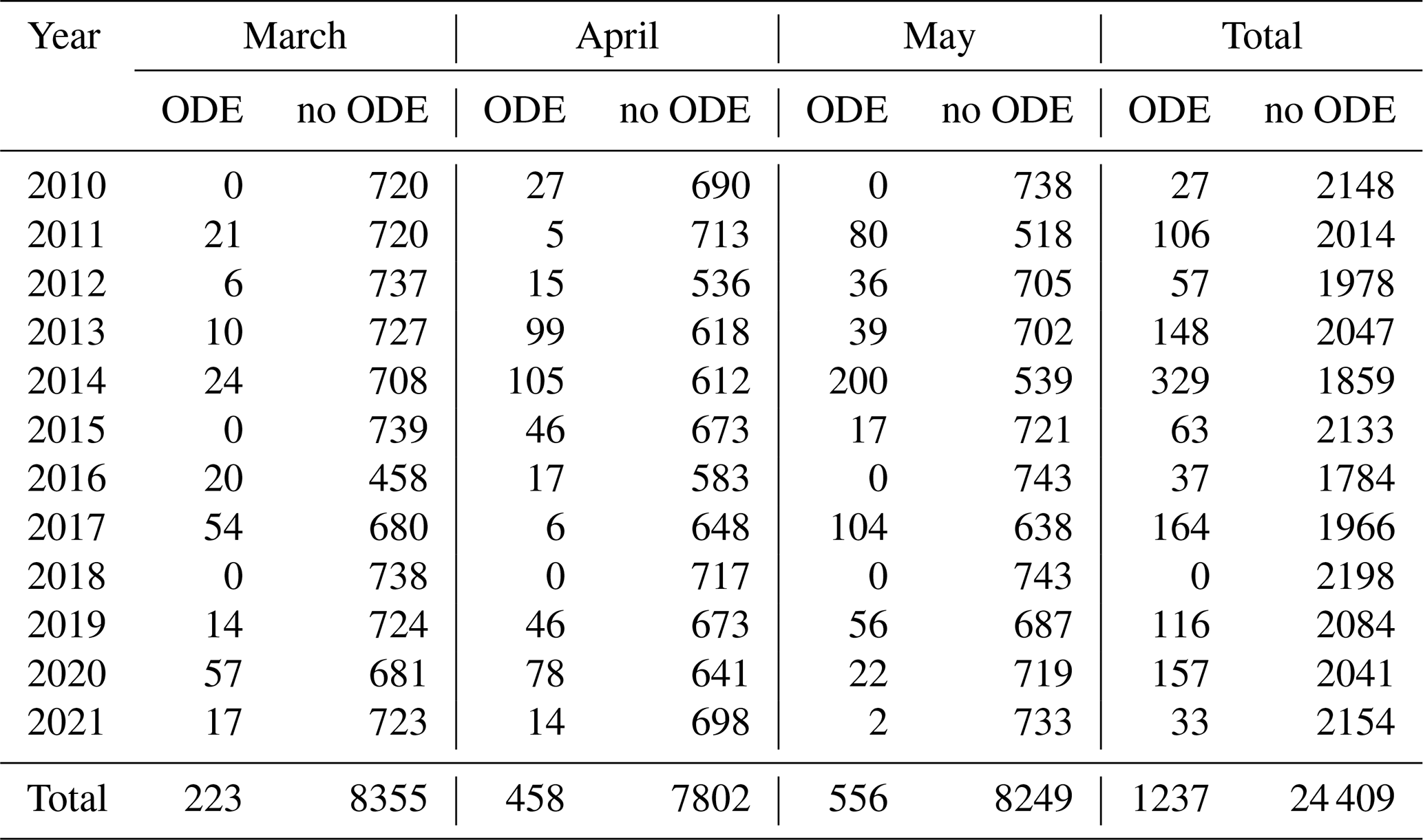
Overall, 242 measurements were taken by ozonesondes and 24 406 h of ozone were monitored at the Zeppelin observatory. The frequencies of ODEs and no ODEs are listed in Table 1 for the sonde and Table 2 for the Zeppelin data set. Note that Zeppelin ozone data have several data gaps that result in an incomplete number of hours of data per month. Interestingly, on Zeppelin mountain most ODEs were observed in May and the highest number of ODEs per month for 1 year was observed in May 2014 with 200 ODEs. For the ozonesonde data set, most ODEs were found in April. This is probably the result of the decreasing number of sonde launches from March to May, reducing the probability of detecting ODEs in May. The influence of the individual years and months on the analysis is discussed in more detail in Sect. 3.2.
Table 1The number of occurrences of ODEs and no ODEs for each month and year from ozonesonde observations.
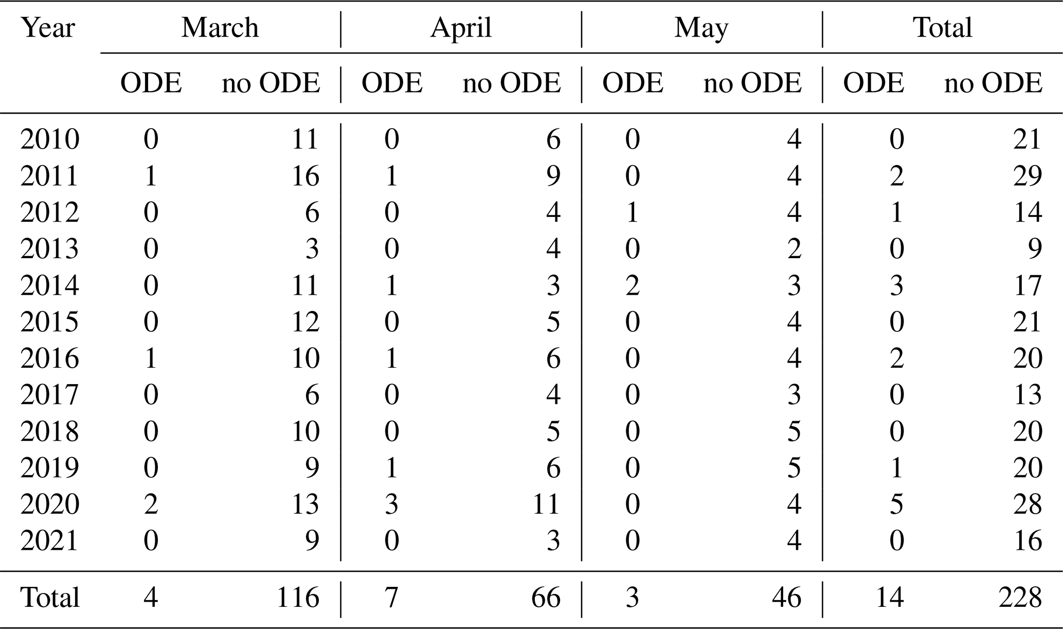
Table 2The number of occurrences of ODE and no ODE for each month and year from hourly in situ ozone measurements at Zeppelin observatory.
2.2 MAX-DOAS BrO profiles from Ny-Ålesund
The IUP Bremen has been operating a DOAS system on top of the roof of the observatory building of the joint French–German Arctic research station in Ny-Ålesund since 1995 (Wittrock et al., 2000). The setup was updated to a two-channel Multi AXis DOAS (MAX-DOAS) system in 1999 (Wittrock et al., 2004). In short, the MAX-DOAS instrument consists of a telescope unit mounted on a pan–tilt head on top of the roof of the observatory that is connected via light fibre to a spectrometer and CCD unit inside the laboratory. Since 1999, routine measurements of scattered sunlight have been performed in several azimuthal directions and at several elevation angles, enabling the analysis of trace gases at a high temporal and spatial resolution. In this study, vertical profiles of BrO concentrations are presented that have been calculated with the inversion algorithm BOREAS (Bösch et al., 2018) from dSCD (differential slant column density) retrieved from elevation scans measured in a northwesterly direction (328∘ clockwise from north).
The vertical sensitivity of MAX-DOAS profile retrievals is highest for lower altitudes and decreases strongly for altitudes larger than 2–3 km (Bösch et al., 2018; Tirpitz et al., 2021). However, elevated trace gas layers can still be retrieved when this layer is the dominant trace gas concentration – no shielding effect of larger near-surface concentrations is present (Tirpitz et al., 2021).
2.3 Satellite observations
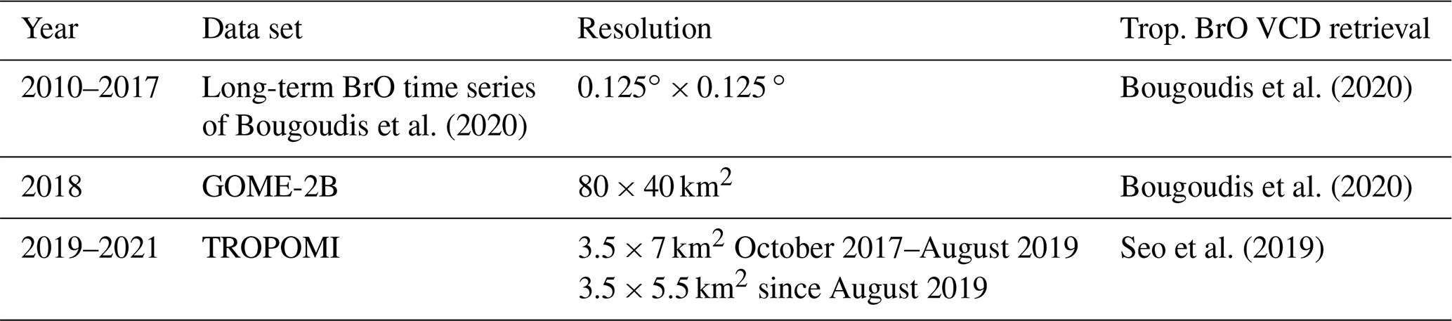
To analyse the distribution of tropospheric BrO in the area of Svalbard during ODEs, three satellite data sets were used and are listed in Table 3. The time period between 2010 and 2017 is covered by the long-term BrO time series of Bougoudis et al. (2020). For this data set, tropospheric BrO north of 70∘ N was derived for a 22-year time period (1996–2017) from four ultraviolet-visible satellite instruments: GOME (Global Ozone Monitoring Experiment), SCIAMACHY (SCanning Imaging Absorption spectroMeter for Atmospheric CartograpHY), GOME-2A, and GOME-2B. For spring 2018, the GOME-2B (Global Ozone Monitoring Experiment-2B) tropospheric BrO data set is used. GOME-2B was launched in 2012 on board the MetOp-B (Meteorological Operational Satellite-B) satellite and belongs to a series of three identical GOME-2 instruments on the platforms MetOp-A, MetOp-B, and MetOp-C (Callies et al., 2000). The time period from 2019 until 2021 is covered by tropospheric BrO from TROPOMI (TROPOspheric Monitoring Instrument), which was launched on board the Copernicus S5P (Sentinel 5 Precursor) satellite in October 2017. Although BrO data from TROPOMI are already available for 2018, these data are not used here due to several data gaps. To obtain the tropospheric SCD (slant column density) of the total BrO column, a stratospheric correction was applied based on Theys et al. (2011). To achieve a consistent BrO analysis, all three data sets were gridded on a 0.125∘ × 0.125∘ grid. A sea ice flagging with EASE-Grid Sea Ice Age data was applied (Tschudi et al., 2019) to analyse only sea-ice-covered areas.
Bougoudis et al. (2020)Bougoudis et al. (2020)Bougoudis et al. (2020)Seo et al. (2019)Table 3Description of the three satellite data sets used to determine daily tropospheric BrO vertical column densities (VCDs) from 2010 to 2021.
2.4 Meteorological and sea ice data
To investigate the meteorological parameters during ODEs, hourly ECMWF ERA5 reanalysis products have been used (Hersbach et al., 2020). Based on earlier studies, the following parameters have been selected: mean sea level pressure (MSLP), planetary boundary layer height (PBLH), temperature at 2 m altitude, and wind speed at 10 m altitude. The data are provided on a latitude–longitude grid of 0.25∘ × 0.25∘.
Daily AMSR (Advanced Microwave Scanning Radiometer) SIC observations on a 25 × 25 km2 grid have been utilized to analyse the sea ice concentration (SIC) around Svalbard as the potential sources region for BEEs (data accessed via https://doi.org/10.24381/cds.3cd8b812, Copernicus Climate Change Service, 2020).
2.5 WRF
In order to study the meteorological conditions for the ODE case study in the beginning of April 2020 and to provide wind fields for the subsequently conducted FLEXPART-WRF runs, the regional Weather Research and Forecasting (WRF) model from the National Center for Atmospheric Research (NCAR) was used (Skamarock et al., 2019). WRF is a mesoscale numerical weather prediction and atmospheric simulation system, and for this case study version 4.2 was applied.
To capture the full development of the ODE during the case study, the model run starts on 31 March 2020 at 12:00 UTC and ends on 3 April 2020 at 12:00 UTC. The model run was initialized using NCEP (National Centers for Environmental Prediction) FNL (Final) Operational Global Analysis data with a 6 h time step and 1 ∘ spatial resolution (data accessed via https://doi.org/10.5065/D6M043C6, National Centers for Environmental Prediction, National Weather Service, NOAA, and U.S. Department of Commerce, 2000). To achieve a reasonable pixel size compared to the TROPOMI resolution, two domains were used (see Fig. 2) in a two-way nested run. The first domain has a size of 6400 × 6400 km2 with 20 × 20 km2 resolution centred over the North Pole covering the whole Arctic region. The second domain is located within the first one and contains the region of interest in a 3924 × 3924 km2 domain with a 4 × 4 km2 resolution centred north of Svalbard. Both domains were projected on a polar stereographic map. The WRF output is given in 30 min time steps. The planetary boundary layer scheme from Mellor–Yamada–Janjić was applied in the model setup (Janjić, 1994).
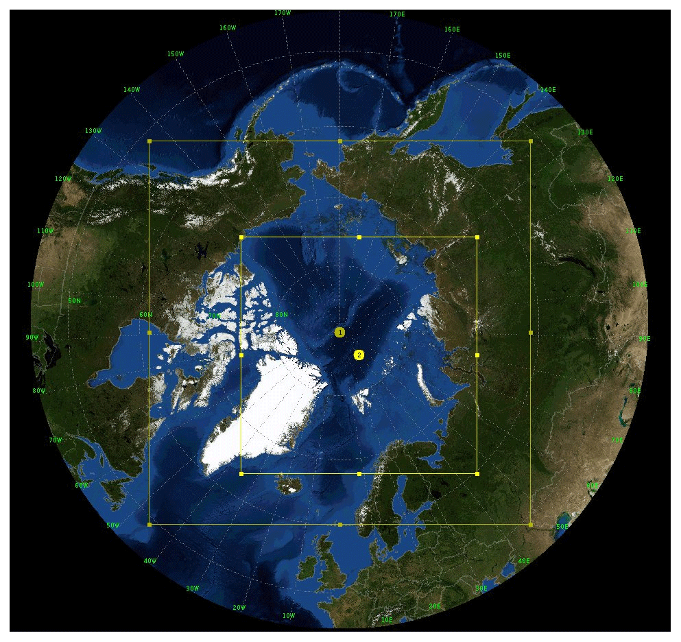
Figure 2The first WRF domain (outer yellow box) centred over the North Pole and the second WRF domain (inner yellow box) centred north of Svalbard.
2.6 FLEXPART-WRF
The Lagrangian trajectory model FLEXPART-WRF (Brioude et al., 2013) (https://www.flexpart.eu/wiki/FpLimitedareaWrf, last access: 22 July 2022), a version of the model FLEXPART (Stohl et al., 2005) driven by WRF meteorological output data, is applied to track the route of the air masses before their arrival in Ny-Ålesund by using particles released in the model. Therefore, the model runs backward in time using the wind fields of two WRF model runs. The first run is very similar to the one described above (see Sect. 2.5) but with a different start and end time (here: 30 March 2020 at 12:00 UTC until 2 April 2020 at 12:00 UTC). For the second one, the same WRF run as described above is used. To define the release altitude and time of the two FLEXPART-WRF runs, the two ozonesonde measurements of 2 and 3 April are used. In total, 200 000 particles are released in one grid box (about 50 × 50 m) containing the ozonesonde release station at the altitude region, where ozone values below 15 ppb were measured. The FLEXPART-WRF output is written on the same spatial grid as the WRF wind fields and at a 30 min time step.
2.7 Method: composite analysis
To investigate the anomalies of (1) meteorological conditions, (2) BrO, and (3) SIC in the Arctic region during ODEs in Ny-Ålesund, a composite analysis was conducted. In a first step, the two ozone data sets were separated individually into ODEs and no ODEs (see Sect. 2.1). For the 15 ppb threshold, we found 14 ODEs and 228 no ODEs in the ozonesonde data set (see Table 1) and 1237 ODE and 24 409 no ODE hours in the Zeppelin data set (see Table 2). In a second step, the time-corresponding meteorological, BrO, and SIC values were selected and averaged. The anomalies were calculated by subtracting the averaged values based on the ODE points in time () from the averaged values based on the no ODE points in time ():
where Y represents the meteorological parameter, BrO, or SIC.
To investigate the development of meteorological conditions and BrO, the anomalies 1 and 2 d before and after an ODE were examined. To generate the new points in time, 24 or 48 h were added to or subtracted from the measured ODE and the time-corresponding meteorological and BrO values were selected. The anomalies were calculated by subtracting the averaged parameters from :
3.1 BrO and meteorological conditions during ODEs
In this section, the anomalies of BrO, meteorological conditions, and SIC during ODEs, calculated using Eq. (1), are discussed. The BrO anomalies in Fig. 3 show enhanced tropospheric BrO vertical column densities (VCDs) during ODEs in Ny-Ålesund for both data sets. The area north of Svalbard shows a positive BrO VCD anomaly of about 2.0×10¹³ molec. cm−2, and overall in the Arctic region slightly increased BrO values are noticeable. This indicates that during ODEs in Ny-Ålesund, BrO levels are enhanced both locally and in the larger Arctic region.
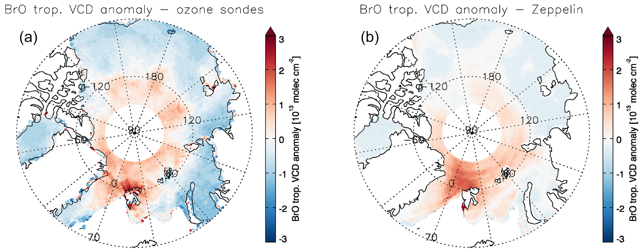
Figure 3Tropospheric BrO VCD anomalies using an ozone threshold value of 15 ppb based on the (a) ozonesonde data set and (b) Zeppelin data set.
As already mentioned in Sect. 1, there are two meteorological conditions stated by Jones et al. (2009) favouring the release of Br2 from the cryosphere and thus BEEs: (1) low wind speeds and a stable boundary layer and (2) high wind speeds with blowing snow and a higher, unstable boundary layer. Using the composite analysis, the systematic anomalies in meteorological parameters during ODEs in Ny-Ålesund can be investigated. The results are summarized in Fig. 4 for both ozone data sets. The first row in Fig. 4 shows that during ODEs a low-pressure anomaly is located over the Barents Sea, while the pressure in the Icelandic Low area is anomalously high. Normally, the Icelandic Low would propagate in a northeasterly direction towards the Barents Sea, transporting warmer air from the south to Svalbard. But due to the low-pressure system over the Barents Sea, the northeast propagation is blocked and cold air from the north is now transported to Svalbard. Therefore, this blocking situation due to the anomalously low pressure in the Barents Sea is associated with cold air outbreaks near Svalbard and leads to transport of polar air from the north to Ny-Ålesund. The transport route can also be seen in the increased wind speed (second row in Fig. 4) north of Greenland and southwards into the Fram Strait (area between Greenland and Svalbard). The maximum of the wind speed anomaly is more enhanced in the ozonesonde data set and shows a maximum of about 4 m s−1 west of Svalbard and north of Canada. The maximum in the Zeppelin data set is located at the northeastern coast of Greenland with increased values west of Svalbard. Seo et al. (2020) also showed increased surface wind speed during enhanced BrO periods over the eastern coast of Greenland and prevailing wind directions from the north and west. These findings indicate that Br is likely recycled on aerosol or blowing snow on its way to Ny-Ålesund, and therefore ozone is continuously depleted along the trajectory to and in Ny-Ålesund. A lifting at the front of the low-pressure system leading to an increase in the PBLH can be seen in the third row. Interestingly, the temperature anomalies show low values during ODEs only around the area of Svalbard, and in the Zeppelin data the whole northern part of the Arctic is even slightly warmer. Our findings align with the results of Seo et al. (2020), who found slightly positive temperature anomalies in the central Arctic region and lower temperatures over the Svalbard area during enhanced BrO events. The lower temperatures over the Svalbard area favour the BEE reaction cycle mechanism (Sander et al., 2006) and thus contribute to the depletion of ozone. It should be taken into account that the overall temperature increases from March until May, and therefore seasonal effects might also play a role here, which is further discussed in Sect. 3.2.
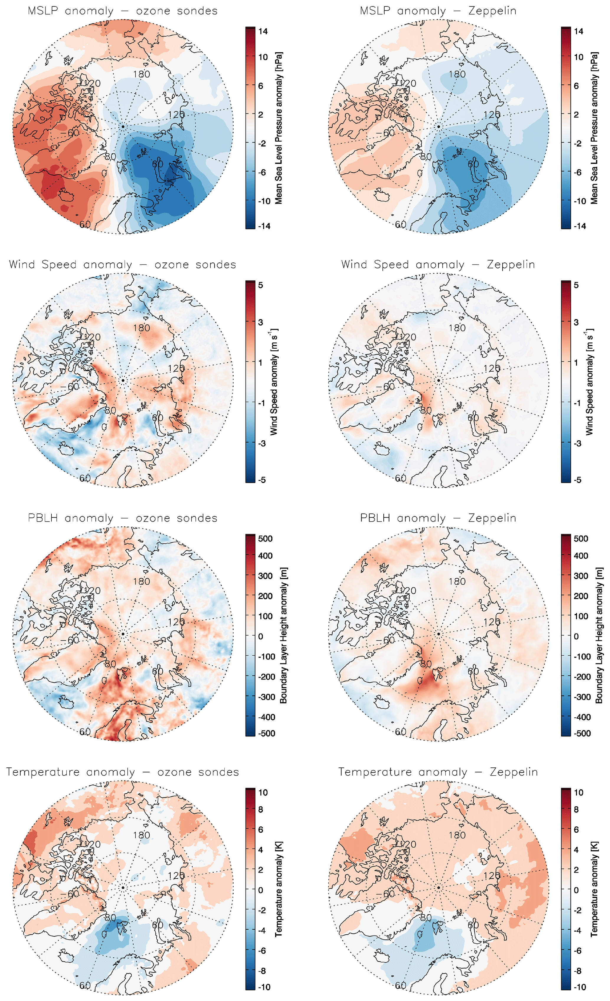
Figure 4MSLP, wind speed, PBLH, and temperature anomalies using an ozone threshold value of 15 ppb based on the ozonesonde data set (left column) and Zeppelin data set (right column).
In addition, the behaviour of sea ice concentration (SIC) during ODEs was investigated. The cryosphere and especially salty snow or sea ice, such as freshly formed sea ice, are assumed to be an important source of Br2. Figure 5 shows an increase in the SIC on ODE days for both data sets, which would be consistent with Br2 sources in this area. However, seasonal effects must be taken into account since the anomalies are also visible shortly before and after an ODE and can therefore not be directly attributed to an ODE. The figure also includes the sea ice edge (SIC below 15 %) for no ODEs (solid line) and ODEs (dashed line). The sea ice edge (SIE) based on the ozonesonde data (left) is further south, closer to Ny-Ålesund than in the Zeppelin data (right). Possible reasons for the shift in the SIE could be (1) the formation of fresh sea ice due to cold polar air from the north or (2) the strong winds from the north pushing the SIE further south. A combination of both is also possible.
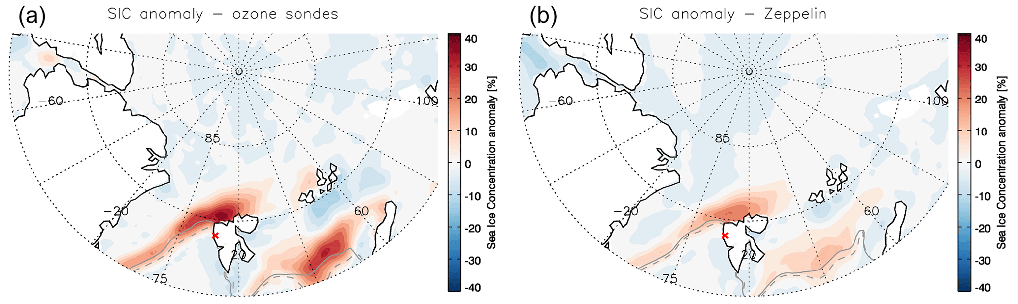
Figure 5SIC anomalies for ODE and no ODE data points based on the (a) ozonesonde data set and (b) Zeppelin data set. The red cross marks the location of Ny-Ålesund. The solid grey line marks the mean SIE for no ODE data points, and the dashed grey line marks the mean SIE for ODE data points.
In general, the anomaly patterns are similar between the two data sets, but they are less pronounced in the Zeppelin data set. This may be due to the larger number of measurements and better coverage in April and May, which also might include more ODEs resulting from low wind speeds and a low, stable boundary layer.
To investigate the development of the meteorological conditions and BrO before and after an ODE, the anomalies were additionally examined 1 and 2 d before and after an ODE based on Eq. (2). Due to long computing times for the Zeppelin data set, only the ozonesonde data are used in this analysis. The resulting figures are shown in Appendix A. For BrO (Fig. A1), an increase towards the day of the ODEs can be observed, as can a decrease during the days thereafter. The highest BrO anomaly over the 5 d period is observed mainly north of the Svalbard coast. The MSLP in Fig. A2 shows a lower pressure over and east of Svalbard on the 2 d before the ODEs. The lower pressure migrates to the southwest throughout the examination period. On the days of the ODEs, the western coast of Svalbard lies in between the higher- and lower-pressure areas. In the days after the ODE, the lower pressure moves further southeast, whereas higher pressure from the west migrates over Svalbard. Figure A3 shows an increase in wind speed towards the days of the ODEs, with a maximum in the wind speed anomaly in the area around Ny-Ålesund. On the ODE days, high wind speed anomalies are observed in the area around Ny-Ålesund. On the days after the ODE, only minor wind speed anomalies are visible. The same behaviour is observed for the PBLH (Fig. A4). A maximum anomaly occurs on the ODE days with an increasing trend towards these days and a decrease afterwards. The temperature does not show a clear trend before and after the ODE days (Fig. A5). However, around the days of ODEs there are generally lower temperatures in the area around Svalbard.
This leads to the conclusion that ODEs in Ny-Ålesund are often induced by polar cyclones migrating from the northeast towards Svalbard. This causes an elevated, unstable PBLH, with higher wind speed and presumably blowing snow where Br can be recycled and transported to Ny-Ålesund depleting ozone on its way to and in Ny-Ålesund.
3.2 Sensitivity and temporal analysis
3.2.1 Analysis of different threshold values
In this section, the influence of the ozone threshold on the composite analysis is discussed. The same method as above is applied but with a threshold of 20 ppb instead of 15 ppb. This leads to 29 ODE and 213 no ODE days in the ozonesonde data set (difference from the amount of measurements at 15 ppb: 15) and 2157 ODE and 23 489 no ODE hours for the Zeppelin data set (difference from the amount of measurements at 15 ppb: 920). The results for BrO and the meteorological conditions are shown in Fig. 6 for the Zeppelin data set and in Fig. B1 for the ozonesonde data set. Compared to the results for 15 ppb shown in Fig. 3 for BrO and Fig. 4 for the meteorological conditions, only minor differences are noticeable for the Zeppelin data set. The BrO anomaly in the 20 ppb data set north of Svalbard is slightly less pronounced than in the 15 ppb data set. The same pattern is also noticeable in the MSLP at the lower-pressure area east of Svalbard and in the PBLH west of Svalbard. The wind and temperature anomalies are almost identical in the area around Svalbard.
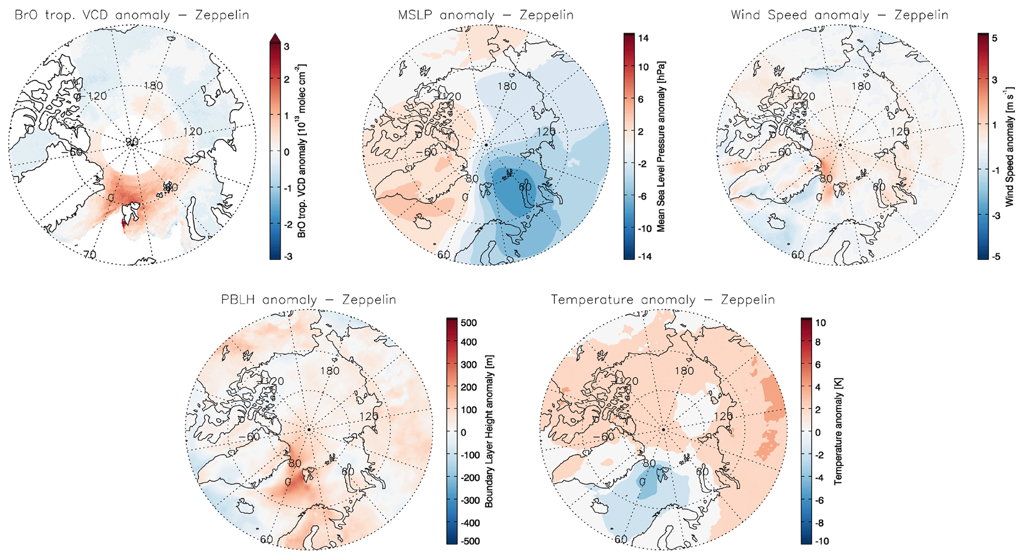
Figure 6Tropospheric BrO VCDs, MSLP, wind speed, PBLH, and temperature anomalies based on the Zeppelin data set using an ozone threshold value of 20 ppb.
For the ozonesonde data set, the differences between the results when using the 15 ppb threshold shown in Fig. 3 for BrO and Fig. 4 for the meteorological conditions and the 20 ppb threshold shown in Fig. B1 are more pronounced compared to the Zeppelin data set. The BrO, PBLH, MSLP, and wind speed anomalies are weaker when applying the 20 ppb threshold. The temperature anomaly around Svalbard is very similar for both ozone thresholds. However, the temperature is warmer throughout the Arctic region at ODEs for the 15 ppb threshold. This may be explained by the increase in the number of ODEs in March when using the 20 ppb threshold, where the temperature in the Arctic is lower than in May.
To investigate if a stronger separation between ODEs and no ODEs alters the observed anomalies, a threshold of 40 ppb for no ODEs was set in addition to the threshold of 15 ppb for ODEs. This evaluation was solely based on the Zeppelin data. A minor rise in BrO, MSLP, PBLH, and temperature anomalies is evidenced in the results not displayed here. Hardly any changes can be seen in the wind speed anomalies. Setting a no ODE threshold removes the weaker ODEs from the no ODE data set and increases anomalies, but the local distribution of the anomalies remains constant for all parameters.
Overall, the anomalies are slightly less pronounced in both data sets when using the 20 ppb threshold, but no major differences in BrO and meteorological anomalies are observed when changing the ozone threshold value. Introducing a limit for no ODEs follows a similar structure. Here, the anomalies slightly increase. We therefore conclude that our analysis is robust with respect to the choice in separation thresholds.
3.2.2 Analysis of anomalies by month
To analyse the influence of seasonal effects, March, April, and May data were analysed separately between 2010 and 2021 for both data sets. Figure 7 shows the results for the Zeppelin data set. The results for the ozonesonde data set are shown in Fig. C1. In the BrO anomalies based on the Zeppelin data set, a decrease in BrO is visible between March and May. High anomalies are visible in March mainly north of Svalbard. In April, the BrO anomalies are still positive but not as pronounced and more homogeneously distributed over the Arctic Ocean. The anomalies in May are smaller compared to the other 2 months. This is unexpected, since the largest number of ODEs is observed in May on Zeppelin mountain (see Table 2). In general, it is expected that with increasing temperature at the end of spring the amount of inorganic Br2 released from the cryosphere decreases, and therefore less Br is available to deplete ozone. In the ozonesonde data set, three ODEs are observed in May (see Table 1), and the BrO anomalies in Fig. C1 show that enhanced BrO values are observed throughout the Arctic region for these 2 d. One possible explanation might be that only a few observed ODEs were induced by Br transported to Ny-Ålesund and that mainly locally induced ODEs with low wind speed and stable boundary layer were observed on Zeppelin mountain. A decrease in the anomaly can also be seen in the MSLP. From March to May, the area of the lower-pressure anomaly becomes weaker and smaller. This decrease is connected to the wind speed anomaly, which also decreases, especially northeast of Greenland and west of Svalbard. The temperature anomaly around Svalbard also decreases. Interestingly, in May the region around the North Pole seems to be slightly cooler during ODEs, which is not observed in March or April. Overall, the observed trends towards a decrease in the described anomalies support the assumption that by the end of spring ODEs in Ny-Ålesund might be more often induced locally and not due to transport from the North Pole region. The PBLH anomalies do not show any clear trends for these 3 months. The enhanced values northeast of Greenland in March and April are probably connected to the enhanced wind speed anomalies and support the assumption that air is transported from this area to Svalbard.
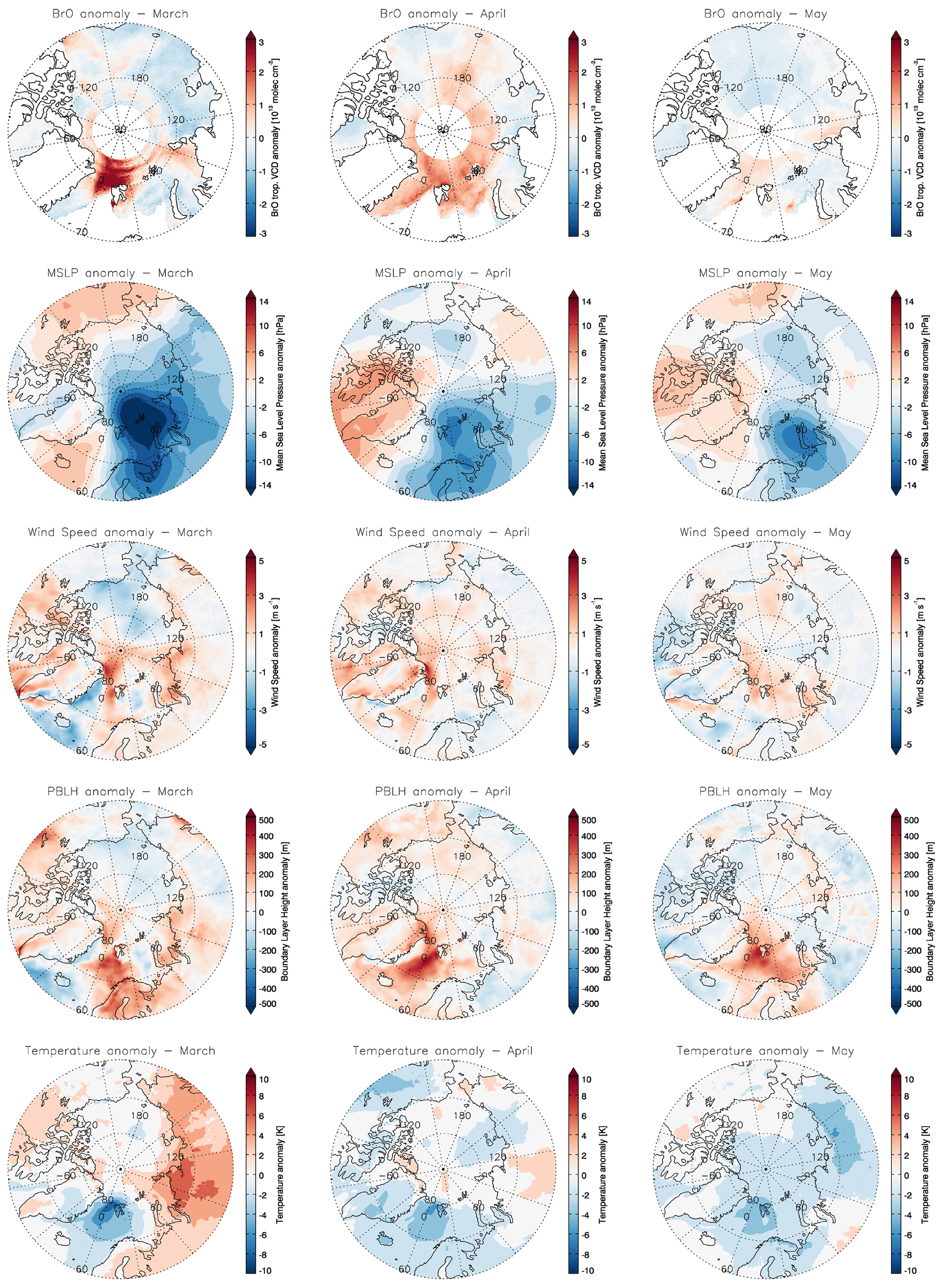
Figure 7Tropospheric BrO VCDs, MSLP, wind speed, PBLH, and temperature anomalies based on the Zeppelin data set for each month: March (left column), April (middle column), and May (right column).
3.2.3 Analysis of anomalies by year
In order to analyse the influence of each year on the results of the composite analysis, a yearly evaluation was performed using the Zeppelin data set. The ozonesonde data set was omitted here because only in 4 of the analysed years was more than one ODE measured (see Table1), which does not lead to robust results. Note that the year 2018 is not included in the analysis because there were no ODEs measured that year (see Table 2). Figure D1 shows the mean BrO anomalies for each year. The years 2016 and 2020 show very high anomalies of BrO north of Svalbard. Except for 2012 and 2015, the other years show enhanced values around the Svalbard region as well, albeit not as strongly as the 2 previously mentioned years. Enhanced values in 2012 are mainly observed in the Fram Strait area and directly on the western coast of Svalbard over Ny-Ålesund. In 2015, enhanced BrO values are visible northeast and east of Greenland and northeast of Svalbard. Overall, each year shows positive BrO anomalies during ODEs, but the years 2016 and 2020 might have the greatest influence on the composite analysis.
The MSLP plots in Fig. D2 show very strong pressure anomalies with lower pressure to the east of Svalbard and higher pressure to the west of Svalbard in the years 2011, 2015, 2016, and 2020. In 2012, 2014, and 2019, a pressure dipole is still visible, albeit not as clearly. For 2017 and 2021, there is a lower pressure overall east and west of Svalbard but more pronounced lower-pressure anomalies on the east side, especially in 2021. No dipole is visible in 2010 and 2013, instead there is only a lower-pressure area north of Svalbard. It can be concluded that a lower-pressure area east and/or a higher-pressure area west of Svalbard can be seen during ODEs in most years, leading to a transport of cold polar air from the north to Svalbard.
These observations are consistent with the results of the wind speed plotted in Fig. D3. In 2010, where no MSLP anomaly dipole was observed, negative wind speed anomalies are obtained. It is the only year where lower wind speeds are observed during ODEs. Additionally, it is the year with the smallest number of observed ODEs other than 2018. Besides 2011 and 2014, which show hardly any change in wind speed close to Ny-Ålesund during ODEs, for every other year increased wind speeds are observed. For the years with positive wind speed anomalies it is very likely that recycled Br and/or ozone-depleted air is transported to Ny-Ålesund, leading to the ODEs. In the areas of enhanced wind speed anomalies, increased PBLH anomalies are visible in Fig. D4 as well.
The temperature anomalies for each year in Fig. D5 consistently show lower temperatures in the area west of Svalbard during ODEs. This finding supports the assumption that lower temperatures accelerate the Br2 release from the cryosphere and therefore can deplete ozone in a sunlit atmosphere. In addition, a seasonality of the temperature is observed in the plots. In years where most of the ODEs took place in May, the Arctic region shows overall positive temperature anomalies, except for the region around Svalbard. On the other hand, in years such as 2016 where most of the ODEs occurred in March, a continuous negative temperature anomaly is observed due to the lower temperatures in March compared to May.
Overall, there is a strong inter-annual variability. Some years have low numbers of ODEs compared to others but show strong anomalies (e.g. 2016), while the year with the most ODEs (e.g. 2014) shows weaker anomalies. Several years, including 2015, 2016, and 2020, show strong anomalies, which significantly influence the composite analysis presented in Sect. 3.1. However, other years still show a similar pattern of anomaly, albeit in a weakened form. Some years, such as 2010 and 2013, show different anomaly patterns in terms of MSLP and wind but still have lower temperature values on ODE days. It might be possible that in years with ODEs in late spring, where no strong MSLP dipole is visible, ODEs might be induced due to a temperature drop that leads to the formation of new sea ice in the area very close to Ny-Ålesund (e.g. Kongsfjorden), where Br2 is emitted locally and initiates the ozone depletion cycle. Another possibility could be sea spray, which infuses coastal snow with salty aerosols, and a subsequent temperature drop can then initiate the bromine reaction cycle.
3.3 ODE case study
At the beginning of April 2020, a major ODE was observed in the ozonesonde observations and in the Zeppelin in situ measurements. The event started around noon on 2 April and lasted for 2 d (see Fig. 8). During these 2 d, ozone was depleted below the detection limit, which is the most severe event recorded between 2010 and 2021. This event occurred in connection with a high-latitude cyclone, a situation which was already discussed in other studies (e.g. Blechschmidt et al., 2016; Chen et al., 2022; Choi et al., 2018). Before the onset of the ODE in Ny-Ålesund, a large comma-shaped BrO plume was observed north of Svalbard in the TROPOMI satellite data on 1 April (see upper left of Fig. 10). The plume arrived in Ny-Ålesund in the afternoon, as recorded by the stationary MAX-DOAS instrument. As shown by the blue line in Fig. 9a, a BrO peak is observed at the same altitude region where a decrease in ozone can be identified. For these 3 d, daily ozonesonde data are available. Ozone was depleted below detection limit in the Zeppelin data for the 2 following days, as well as in the sonde data up to around 1.5 km altitude. Enhanced BrO values were also detected by the MAX-DOAS instrument in the same altitude region (see Fig. 9). For 2 April, the TROPOMI satellite image (see upper middle Fig. 10) shows several BrO hotspots scattered over Svalbard and northeast of Greenland. For the following day, the main plume is partly visible east of Greenland, and only a very weak signal of BrO is visible over Svalbard (see upper right Fig. 10). However, the MAX-DOAS instrument (see Fig. 9c) shows elevated BrO values for that day and ozone is still depleted below the detection limit of the sonde. This leads to the assumption that the amount of BrO is not fully captured by the satellite observations due to lack of sensitivity in detecting local phenomena.
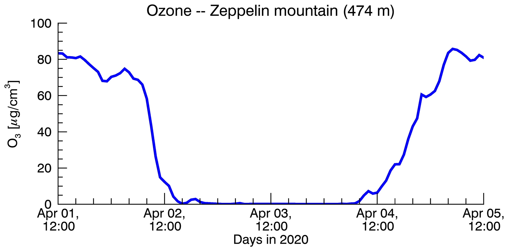
Figure 8Zeppelin ozone data between 1 April at 12:00 UTC and 5 April at 12:00 UTC capturing a major ODE, where ozone is depleted below the detection limit.
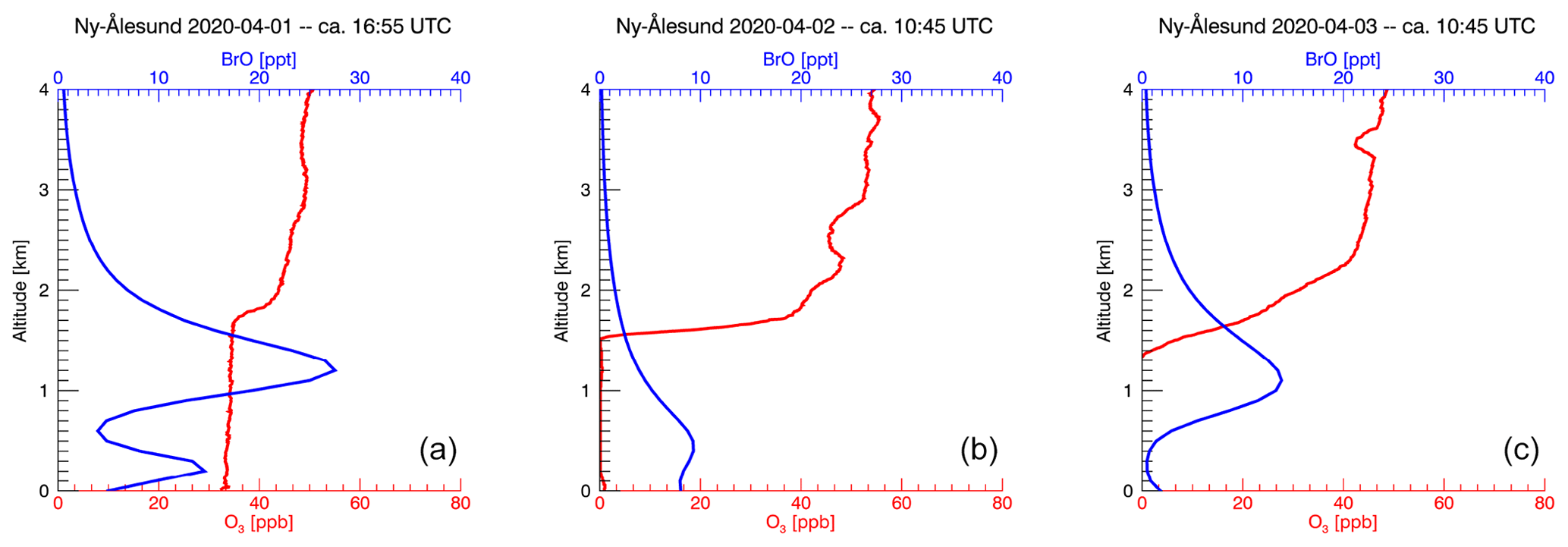
Figure 9Ozonesonde measurements (red) together with BrO MAX-DOAS profiles (blue) for (a) 1 April, (b) 2 April, and (c) 3 April 2020.
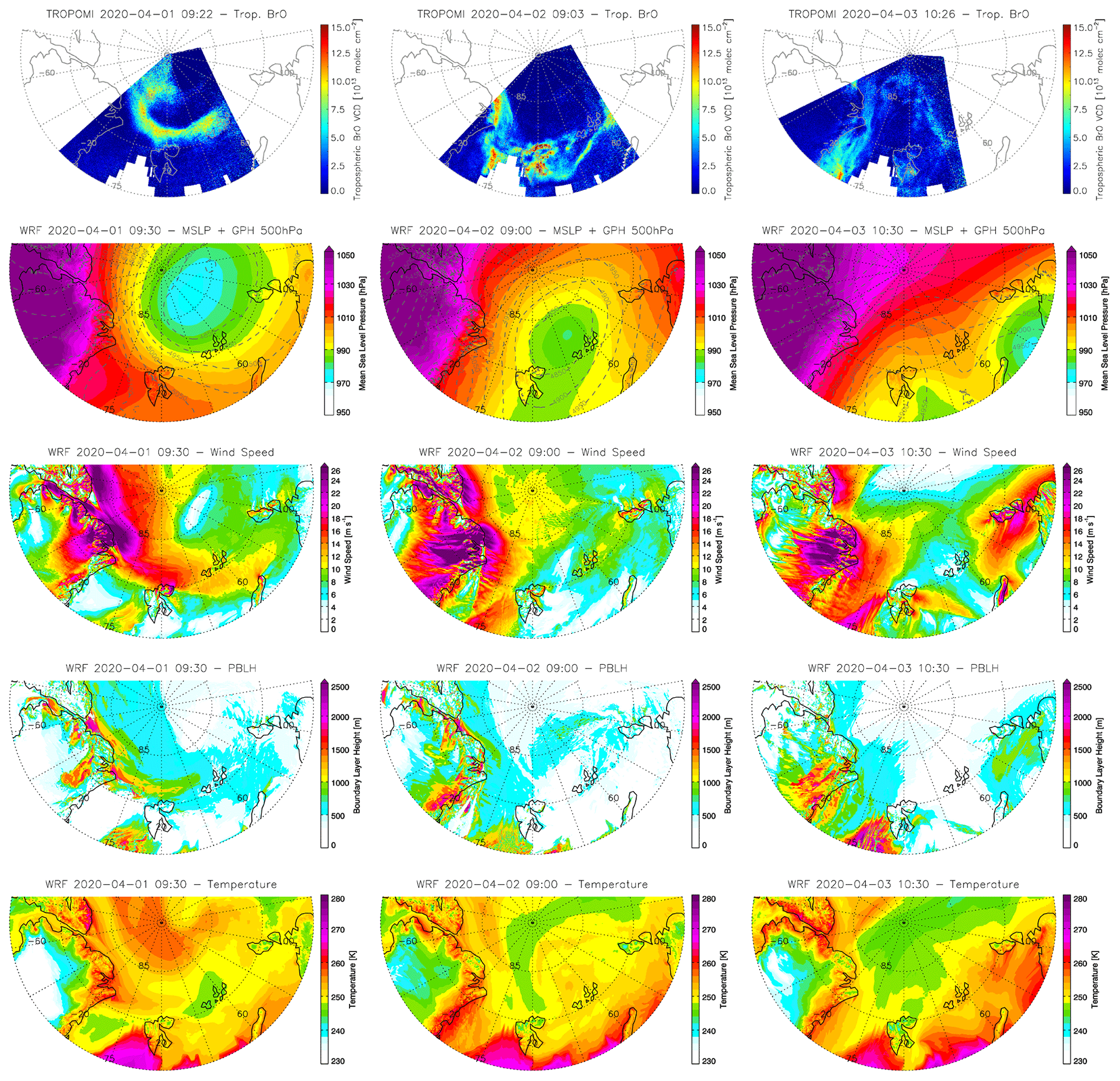
Figure 10(first row) Tropospheric BrO VCD for three satellite overpasses over Svalbard on 1 April (left), 2 April (middle), and 3 April (right). The images below show the WRF output closest in time to the satellite images for MSLP (second row), wind speed (third row), PBLH (fourth row), and temperature (fifth row).
To investigate the meteorological conditions during this event, WRF simulations were conducted as shown in Fig. 10. As in the composite analysis, MSLP, wind speed, PBLH, and temperature are plotted here. For better comparison, the WRF output closest in time to a TROPOMI overpass over Svalbard is used. The simulations show a low-pressure system located northeast of Svalbard on 1 April that propagates southwest towards Svalbard arriving on 2 April. The system then moves over Svalbard and progresses further south on 3 April. The low-pressure system in combination with the high-altitude ozone depletion captured by the ozonesondes corresponds with the findings of Jones et al. (2010), who observed ozone depletion above 1 km in conjunction with a low-pressure system and high wind speed in the Southern Hemisphere. Together with the low-pressure system, there are increased wind speeds at the front of the cyclone, transporting cold polar air southwards. A lifting of the planetary boundary layer at the front of the cyclone can be seen as well. These findings are consistent with the observations in Chen et al. (2022), where it is assumed that the observed BEE in Ny-Ålesund was primarily initiated by blowing snow, presumably covered by brine, triggered by a polar cyclone approaching Svalbard.
Two FLEXPART-WRF backward runs were executed to investigate the origin of the air masses arriving in Ny-Ålesund. The first run was initialized for 2 April and the particles were traced back 3 d (see Fig. 11a). Due to the assumption that the source of Br is salty sea ice and therefore close to the ground, only the trace of the particles within 50 m above sea level is shown here. As can be seen, the particles arriving at Ny-Ålesund originate from the north with the highest sensitivity and therefore a possible source close to Ny-Ålesund. Note that the particles released in the run can either represent Br that depletes ozone or air masses where ozone is already depleted. The ODE could have been induced by local Br or Br that was recycled over the Arctic sea ice and transported to Ny-Ålesund. As another option, ozone-depleted air from the Arctic sea ice arriving at Ny-Ålesund led to the ODE. The second run initialized on 3 April shows a transport route of the particles that follows the shape of the polar cyclone (see Fig. 11b). It is plausible that on this track a lot of ozone depletion occurred and that the air arriving in Ny-Ålesund already contained very little ozone.
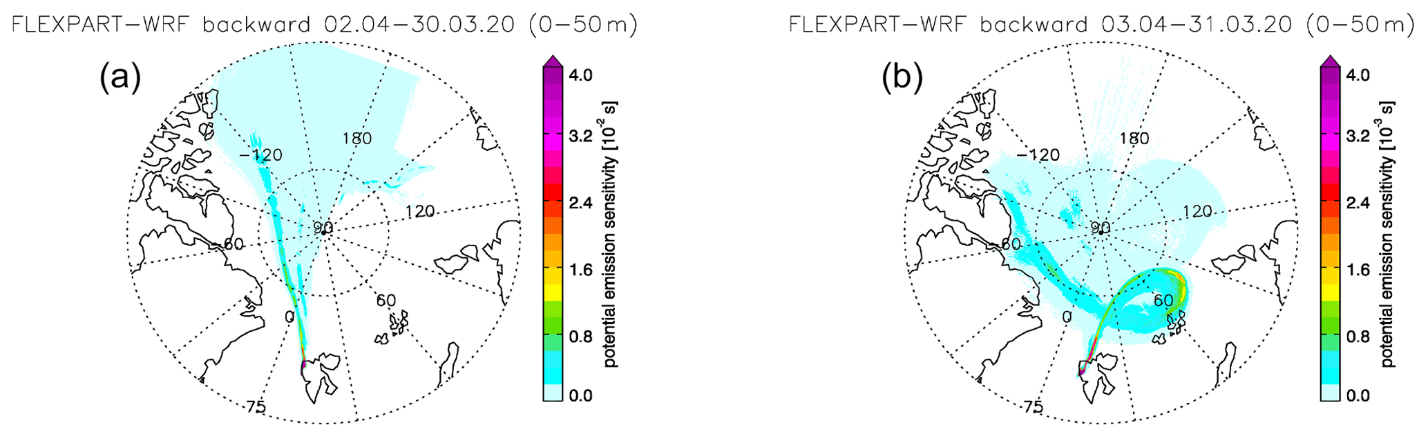
Figure 11Output of two FLEXPART-WRF backward runs initialized on (a) 2 April at 11:00 UTC and (b) 3 April at 11:00 UTC.
In addition, aerosol profiles of the MAX-DOAS instrument and camera images from Zeppelin mountain (https://data.npolar.no/_file/zeppelin/camera/, last access: 12 July 2023) were included to investigate the local conditions and the role of blowing snow during this ODE. The aerosol profiles and camera images both showed high aerosol levels, very likely blowing snow, on 1 April. Enhanced values of BrO are recorded in the afternoon of that day. Therefore, the blowing snow was already present when the plume arrived. The data from 2 and 3 April did not show any signs of enhanced aerosols in the MAX-DOAS profiles. After 1 April, according to the images from Zeppelin mountain, a new layer of sea ice was formed in Kongsfjorden. Therefore, ozone depletion of local Br origin from the freshly formed sea ice is likely to have happened on 2 and 3 April. This case study nicely illustrates the ODE conditions found by the results of the composite analysis. A low-pressure system from the northeast approaching Svalbard led to high wind speeds and low temperatures transported from the north to Ny-Ålesund and resulted in increased BrO values and a severe ODE.
This study investigated the meteorological conditions that are associated with ODEs occurring in Ny-Ålesund during the period 2010–2021. A composite analysis was performed using two different ozone data sets: the ozonesonde record and the hourly in situ observations at the Zeppelin observatory. The composite analysis showed that ODEs are linked to an atmospheric blocking situation, with a low-pressure anomaly located over the Barents Sea and anomalously high pressure in the region of the Icelandic Low. This leads to the transport of cold polar air from the north to Ny-Ålesund, with higher wind speeds potentially inducing blowing snow along the way. The PBLH is anomalously high in the areas of higher wind speed. In addition to the pressure and wind anomalies, lower than normal temperatures are found around Svalbard during ODEs as well as enhanced BrO columns. Since the coastal area around Ny-Ålesund and Kongsfjorden is mostly sea ice free in spring nowadays, air depleted in ozone and enriched in BrO is probably transported to Ny-Ålesund. During the long-range transport over the sea-ice-covered areas north of Svalbard, recycling of bromine on blowing snow is possible. Analysis of the days before and after an ODE showed the development of a polar cyclone with the highest anomalies in pressure, wind speeds, PBLH, and temperature on the day of the ODE and decreasing anomalies thereafter.
To analyse the robustness of the results, both data sets were additionally evaluated with a higher ozone threshold value of 20 ppb. For both data sets the anomalies were slightly less pronounced at the 20 ppb threshold, with the differences in the ozonesonde data set being slightly larger than in the Zeppelin data set. It is assumed that the ODEs in Ny-Ålesund also become less pronounced with weaker weather systems.
The monthly analysis showed a decrease in the anomalies towards May in the Zeppelin data set. This leads to the assumption that in early spring and mid-spring ODEs near Ny-Ålesund are induced more often by low-pressure systems with high wind speeds and cold air masses transported from the north. In late spring (around May), ODEs are probably more often induced during calm meteorological conditions where bromine can accumulate and deplete ozone. Possible sources could be sea spray that infuses coastal snow with sea salt aerosols that at a sufficiently low temperature releases bromine to the troposphere. Another option might be that fresh sea ice is formed locally due to a temperature drop, serving as bromine source. Alternatively, ozone-depleted air from the north can still be transported to Svalbard, leading to ODEs without local ozone depletion chemistry.
The annual evaluation shows that several individual years present similar patterns of anomalies to the combined data set. These years have the strongest influence on the overall outcome of the composite analysis. Some years show only weak anomaly patterns or have a different anomaly pattern. This applies especially for MSLP, wind, and PBLH. However, all years have in common that there are lower temperatures in Ny-Ålesund during ODEs and higher BrO columns upwind of the station.
Finally, a case study in the beginning of April 2020 was introduced when ozone was depleted below the detection limit for 2 d. The ODE occurred in conjunction with a low-pressure system arriving at Svalbard from the northeast with high wind speeds and transport of cold polar air from the north. It showed similar meteorological patterns to the anomalies of the composite analysis and is an example of how these conditions can lead to severe ODEs in Ny-Ålesund. It is very likely that most of the ozone-poor air and BrO was transported to Ny-Ålesund with recycling of BrO over the sea ice region. In summary, the majority of ODEs in Ny-Ålesund appear to be driven by meteorological conditions favouring transport of cold polar air to Svalbard, particularly in early spring. With regard to the rising temperatures in the Arctic (Serreze and Barry, 2011), the consequences of changes in the meteorological parameters and SIC due to rising temperatures on halogen release from the cryosphere require further investigation. The evolution of the quantity and strength of BEEs and consequently of ODEs in relation to changing meteorological drivers will be a future topic of discussion.
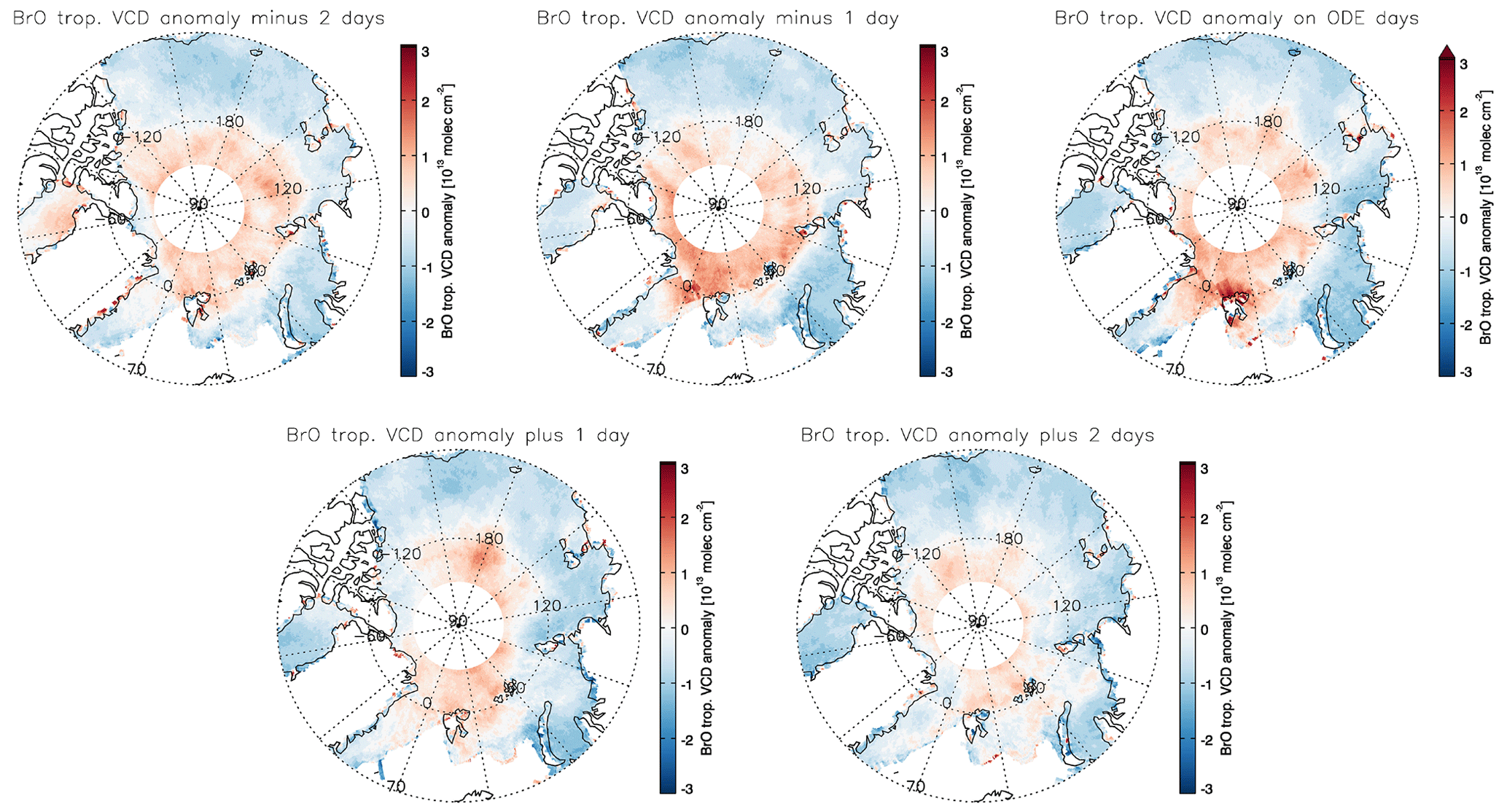
Figure A1Tropospheric BrO VCD anomalies 1 and 2 d before and after the ODE and the day of the ODE based on the ozonesonde data set.
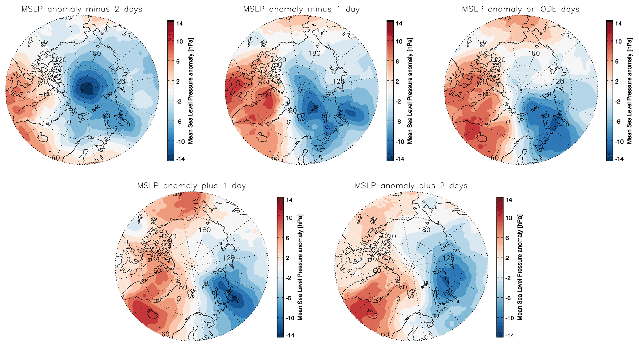
Figure A2MSLP anomalies 1 and 2 d before and after the ODE and the day of the ODE based on the ozonesonde data set.
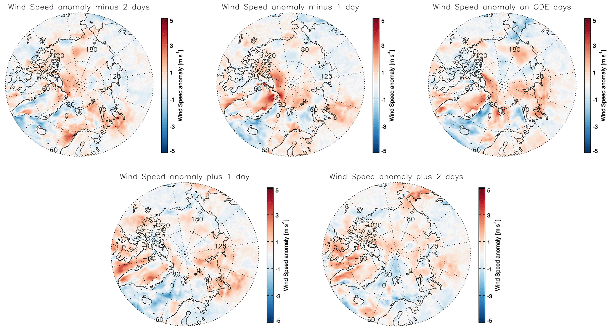
Figure A3Wind speed anomalies 1 and 2 d before and after the ODE and the day of the ODE based on the ozonesonde data set.
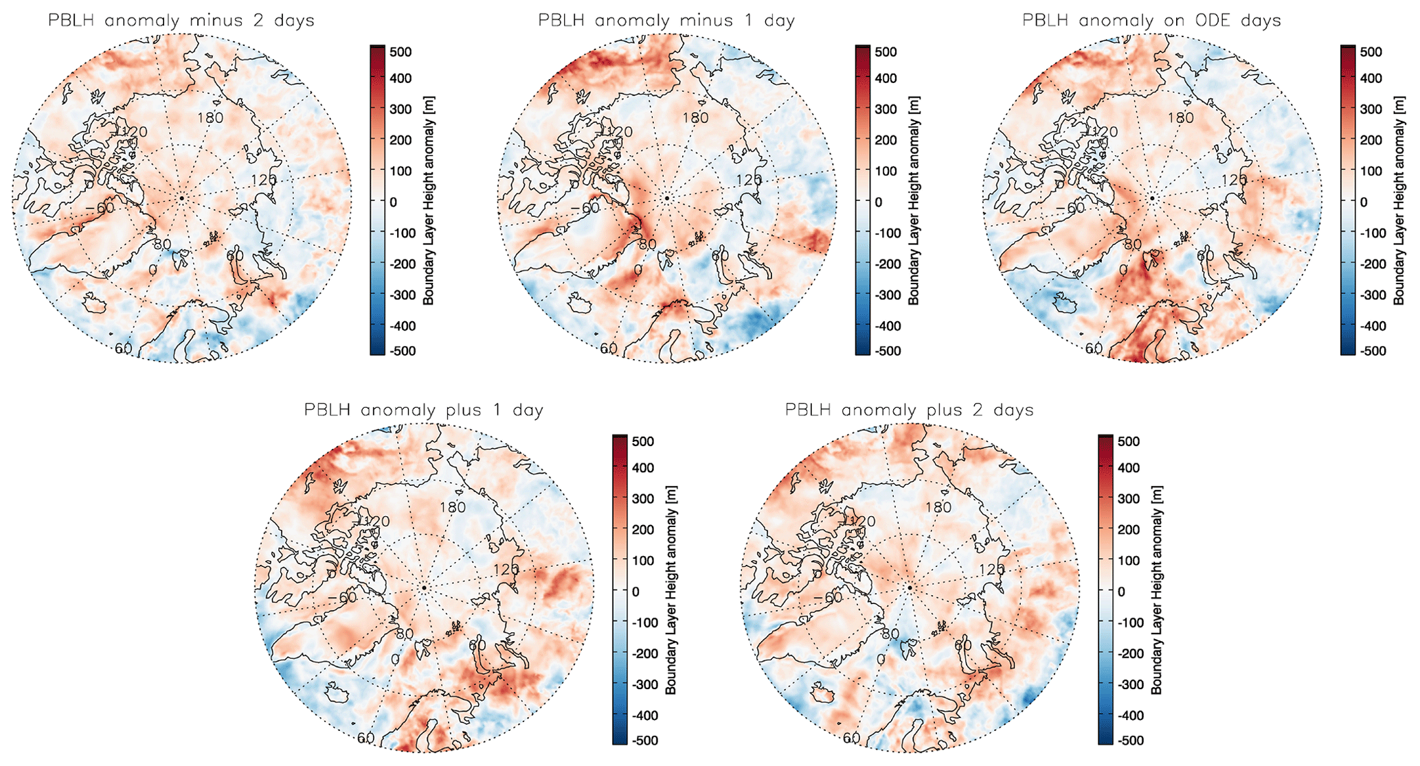
Figure A4PBLH anomalies 1 and 2 d before and after the ODE and the day of the ODE based on the ozonesonde data set.
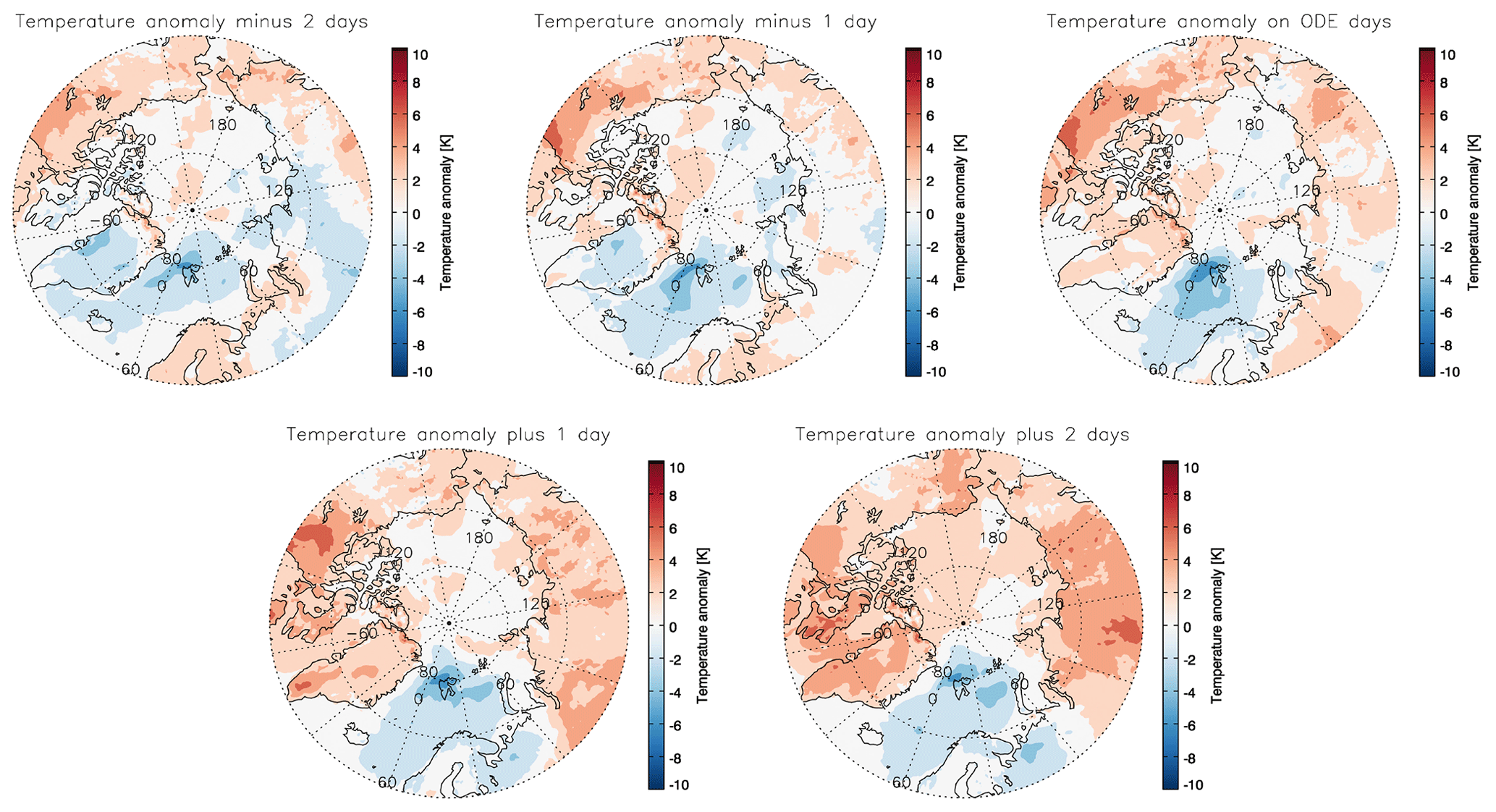
Figure A5Temperature anomalies 1 and 2 d before and after the ODE and the day of the ODE based on the ozonesonde data set.
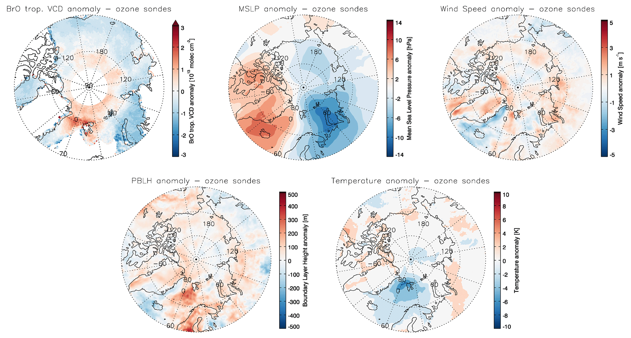
Figure B1Tropospheric BrO VCDs, MSLP, wind speed, PBLH, and temperature anomalies based on the ozonesonde data set using an ozone threshold value of 20 ppb.
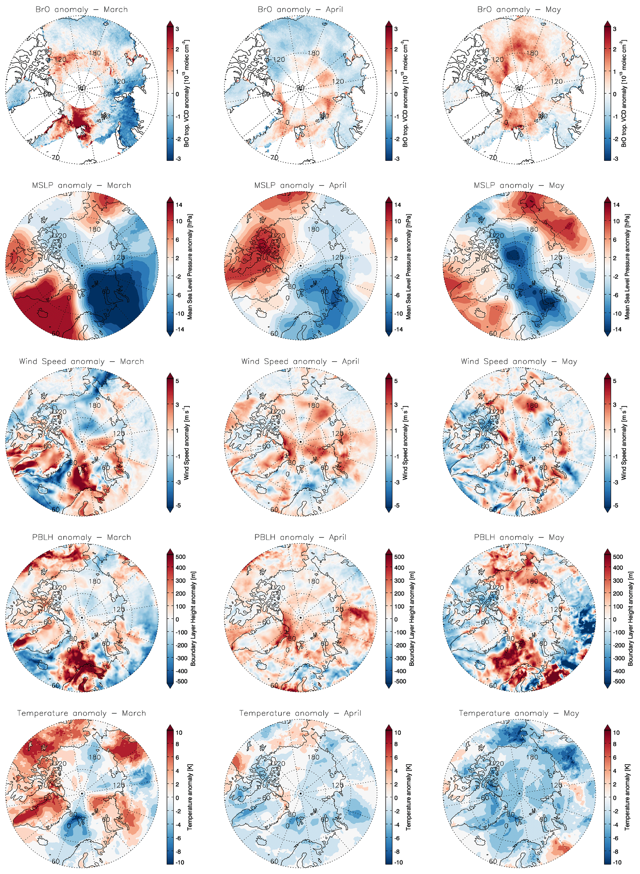
Figure C1Tropospheric BrO VCDs, MSLP, wind speed, PBLH, and temperature anomalies based on the ozonesonde data set for each month: March (left column), April (middle column), and May (right column).
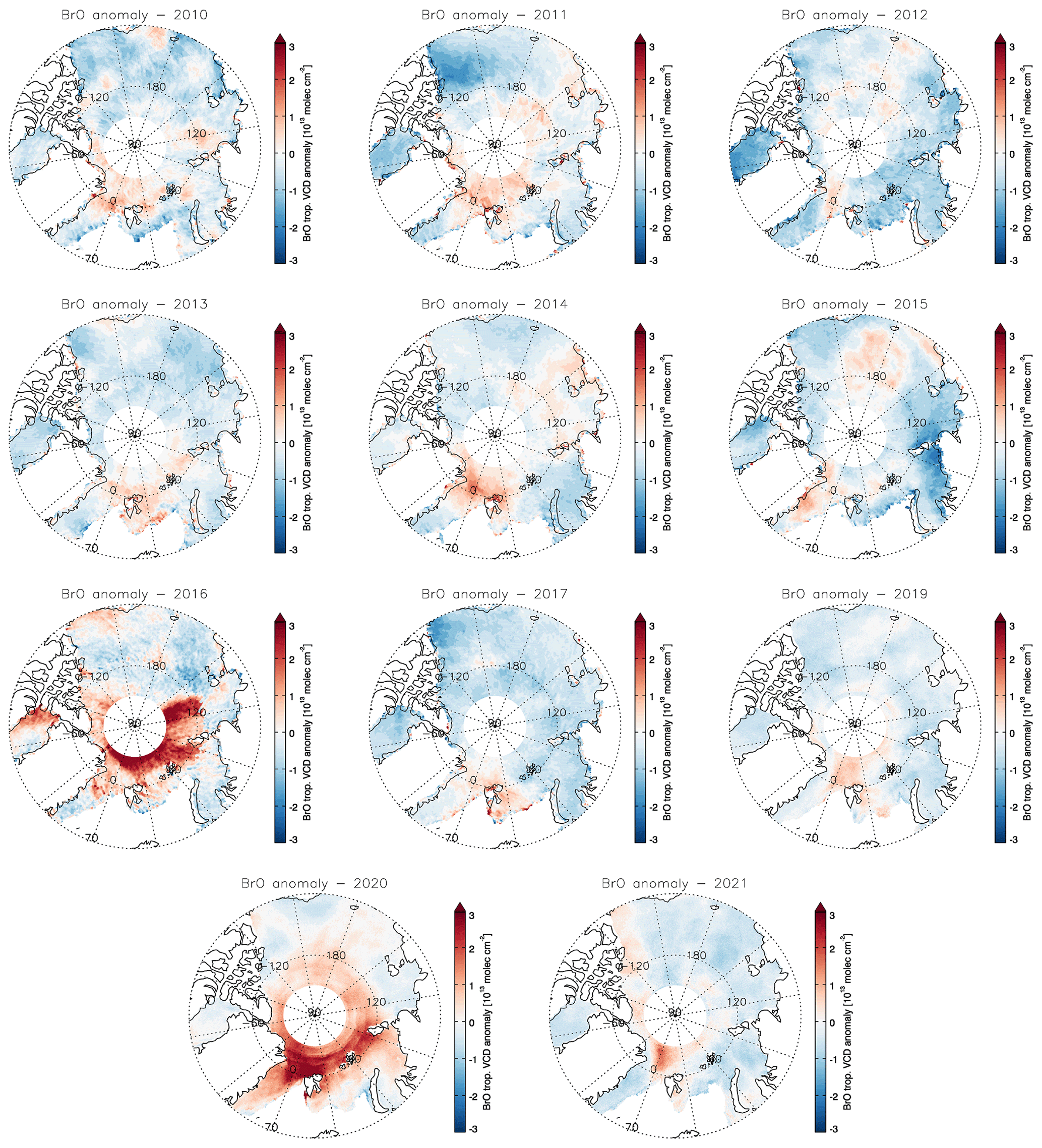
Figure D1Tropospheric BrO VCD anomalies based on the Zeppelin data set for each year between 2010 and 2021. No ODEs were measured in 2018, and therefore no anomalies are calculated.

Figure D2MSLP anomalies based on the Zeppelin data set for each year between 2010 and 2021. No ODEs were measured in 2018, and therefore no anomalies are calculated for that year.
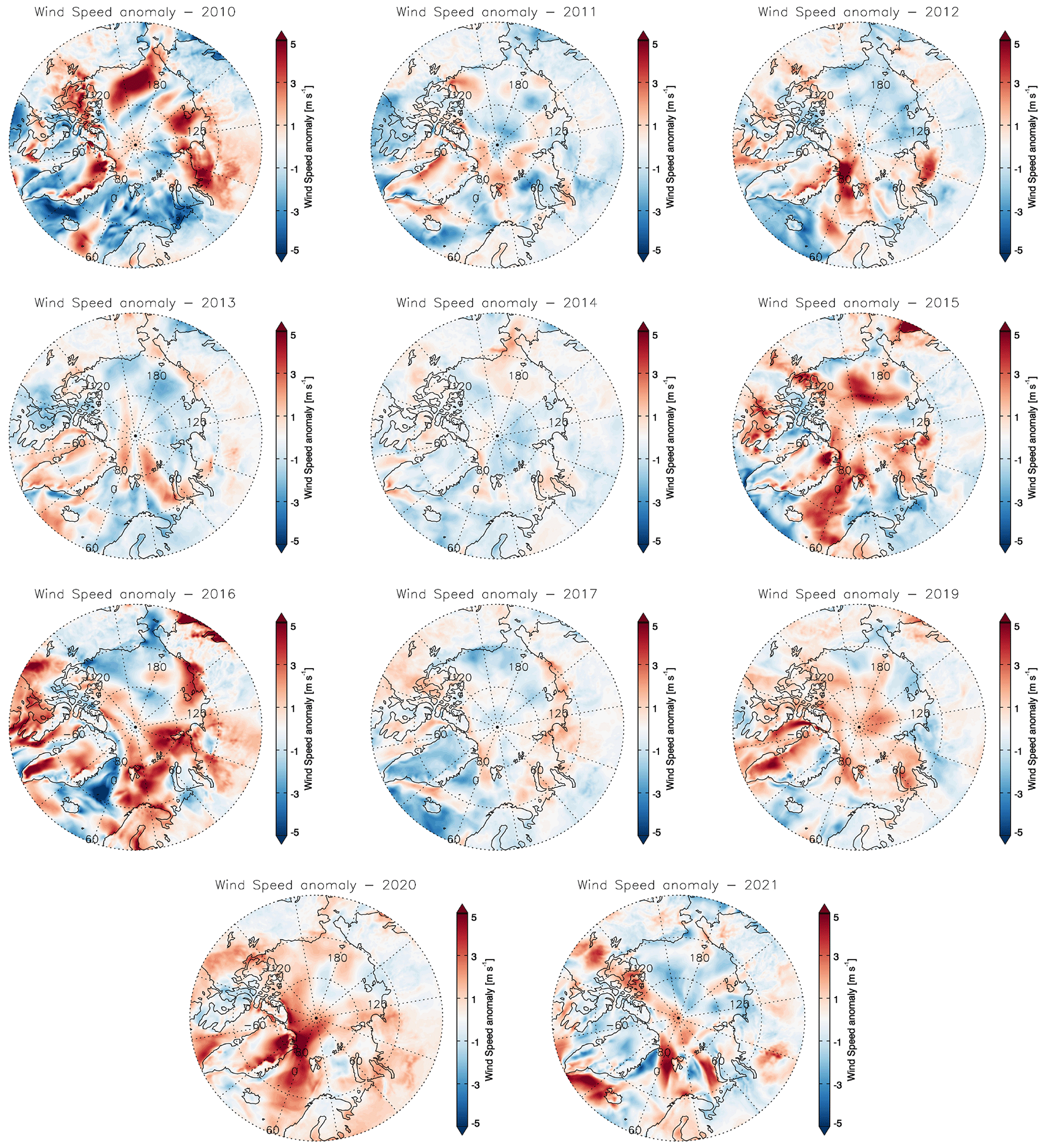
Figure D3Wind speed anomalies based on the Zeppelin data set for each year between 2010 and 2021. No ODEs were measured in 2018, and therefore no anomalies are calculated for that year.
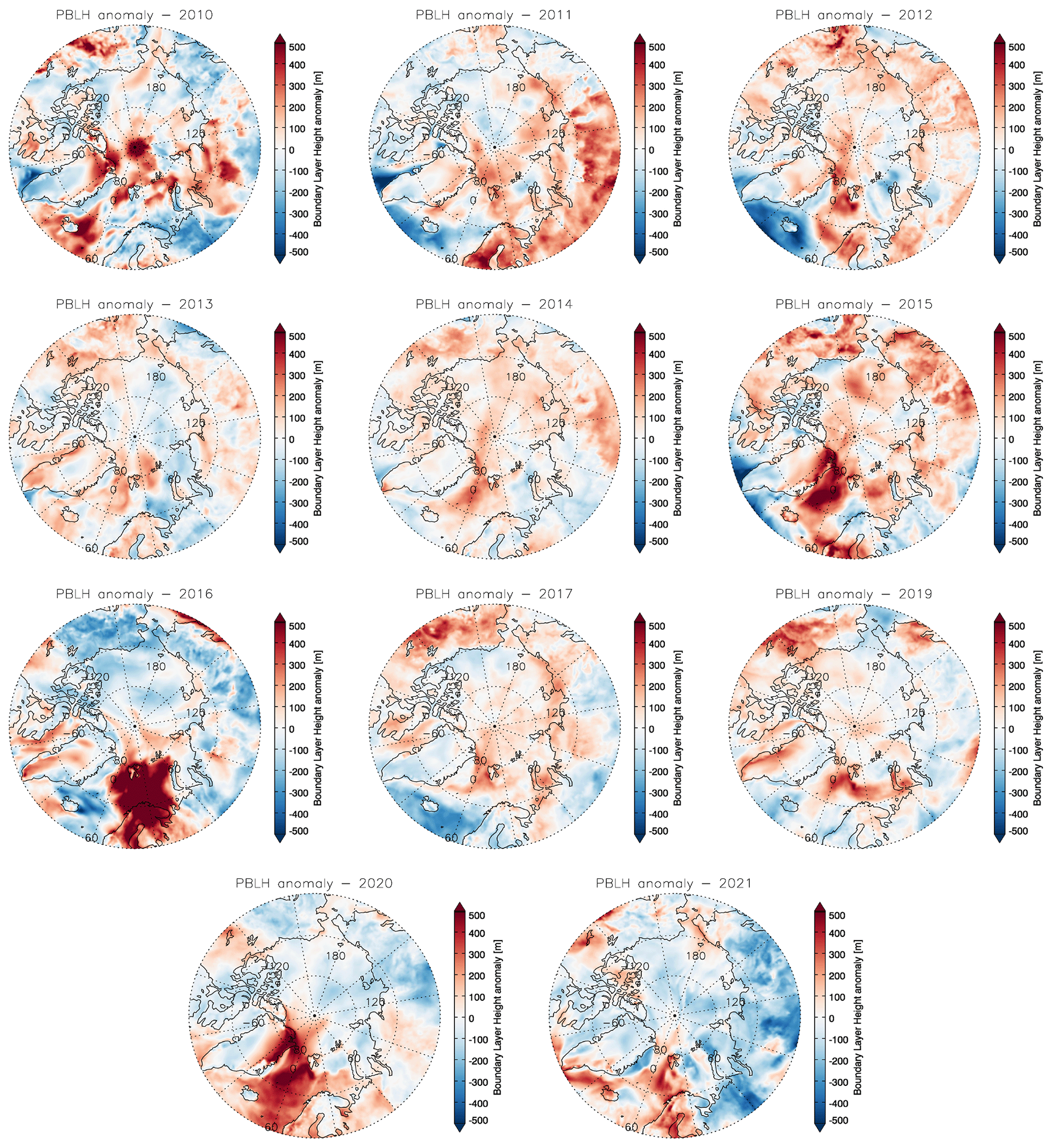
Figure D4PBLH anomalies based on the Zeppelin data set for each year between 2010 and 2021. No ODEs were measured in 2018, and therefore no anomalies are calculated for that year.
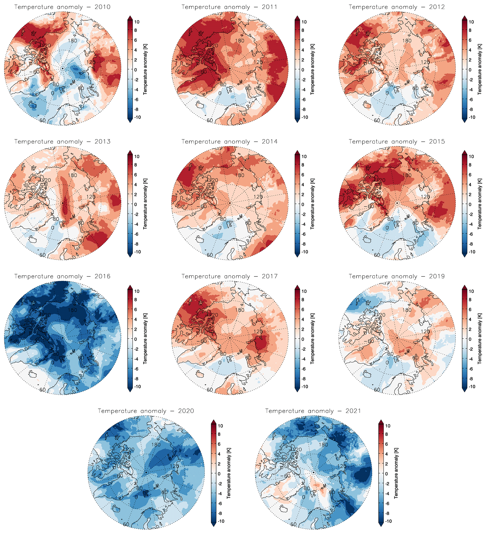
Figure D5Temperature anomalies based on the Zeppelin data set for each year between 2010 and 2021. No ODEs were measured in 2018, and therefore no anomalies are calculated for that year.
WRF source code from the National Center for Atmospheric Research (NCAR) Version 4.2 was accessed via http://www2.mmm.ucar.edu/wrf/users/ (Skamarock et al., 2019). Flexpart-WRF was obtained from their website https://www.flexpart.eu/wiki/FpLimitedareaWrf (Brioude et al., 2013).
Ozonesonde records are available from the Network for the Detection of Atmospheric Composition Change at https://www.ndacc.org (NDACC, 2022). Ozone in situ data from Zeppelin mountain were provided by the Norwegian Institute for Air Research (NILU) at https://ebas-data.nilu.no/ (Platt et al., 2022). ERA5 meteorological and sea ice data are available at ECMWF (Hersbach et al., 2020, https://doi.org/10.1002/qj.3803). EASE-Grid Sea ice Age version 4 data were accessed via https://doi.org/10.5067/UTAV7490FEPB (Tschudi et al., 2019). NCEP FNL data were provided by the Computational and Information Systems Laboratory (CISL) on their website https://doi.org/10.5065/D6M043C6 (National Centers for Environmental Prediction, National Weather Service, NOAA, and U.S. Department of Commerce, 2000). The long-term BrO data set from Bougoudis et al. (2019) is available through the World Data Center PANGAEA at https://doi.org/10.1594/PANGAEA.906046.
This study was designed by BZ, AR, and AB. BZ performed the data analysis and wrote the manuscript with contributions from AR, TB, PvdG, and JB. Data input was provided from PvG, TB, IB, and SS. All authors contributed to the final manuscript.
At least one of the (co-)authors is a member of the editorial board of Atmospheric Chemistry and Physics. The peer-review process was guided by an independent editor, and the authors also have no other competing interests to declare.
Publisher's note: Copernicus Publications remains neutral with regard to jurisdictional claims in published maps and institutional affiliations.
We thank the developers of WRF and FLEXPART-WRF for the model source code that is available on their web pages. Furthermore, we thank ECMWF for providing their ECMWF ERA5 reanalysis products on their website. We thank the team behind the Zeppelin Observatory and EBAS for making their ozone data available on their websites. Additionally, we want to thank the Norwegian Polar Institute for providing the Ny-Ålesund web camera images on their website. The EASE-Grid Sea Ice Age version 4 data were kindly contributed by NSIDC. Parts of the sea ice evaluation were kindly supported by Lars Aue.
This study has been supported by the Deutsche Forschungsgemeinschaft (DFG, German Research Foundation) project no. 268020496-TRR 172, within the Transregional Collaborative Research Center “ArctiC Amplification: Climate Relevant Atmospheric and SurfaCe Processes, and Feedback Mechanisms (AC)3”.
The article processing charges for this open-access publication were covered by the University of Bremen.
This paper was edited by Farahnaz Khosrawi and reviewed by two anonymous referees.
Barrie, L. and Platt, U.: Arctic tropospheric chemistry: An overview, Tellus B, 49, 450–454, https://doi.org/10.3402/tellusb.v49i5.15984, 1997. a
Barrie, L., Bottenheim, J., Schnell, R. C., Crutzen, P. J., and Rasmussen, R.: Ozone destruction and photochemical reactions at Polar sunrise in the lower Arctic atmosphere, Nature, 334, 138–141, 1988. a
Begoin, M., Richter, A., Weber, M., Kaleschke, L., Tian-Kunze, X., Stohl, A., Theys, N., and Burrows, J. P.: Satellite observations of long range transport of a large BrO plume in the Arctic, Atmos. Chem. Phys., 10, 6515–6526, https://doi.org/10.5194/acp-10-6515-2010, 2010. a, b
Benavent, N., Mahajan, A. S., Li, Q., Cuevas, C. A., Schmale, J., Angot, H., Jokinen, T., Quéléver, L. L., Blechschmidt, A. M., Zilker, B., Richter, A., Serna, J. A., Garcia-Nieto, D., Fernandez, R. P., Skov, H., Dumitrascu, A., Sim oes Pereira, P., Abrahamsson, K., Bucci, S., Duetsch, M., Stohl, A., Beck, I., Laurila, T., Blomquist, B., Howard, D., Archer, S. D., Bariteau, L., Helmig, D., Hueber, J., Jacobi, H. W., Posman, K., Dada, L., Daellenbach, K. R., and Saiz-Lopez, A.: Substantial contribution of iodine to Arctic ozone destruction, Nat. Geosci., 15, 770–773, https://doi.org/10.1038/s41561-022-01018-w, 2022. a
Blechschmidt, A.-M., Richter, A., Burrows, J. P., Kaleschke, L., Strong, K., Theys, N., Weber, M., Zhao, X., and Zien, A.: An exemplary case of a bromine explosion event linked to cyclone development in the Arctic, Atmos. Chem. Phys., 16, 1773–1788, https://doi.org/10.5194/acp-16-1773-2016, 2016. a, b
Bösch, T., Rozanov, V., Richter, A., Peters, E., Rozanov, A., Wittrock, F., Merlaud, A., Lampel, J., Schmitt, S., de Haij, M., Berkhout, S., Henzing, B., Apituley, A., den Hoed, M., Vonk, J., Tiefengraber, M., Müller, M., and Burrows, J. P.: BOREAS – a new MAX-DOAS profile retrieval algorithm for aerosols and trace gases, Atmos. Meas. Tech., 11, 6833–6859, https://doi.org/10.5194/amt-11-6833-2018, 2018. a, b
Bougoudis, I., Blechschmidt, A.-M., Richter, A., Seo, S., and Burrows, J. P.: Climatologies of Geometric and Tropospheric BrO Vertical Column Densities derived from multiple UV-Vis Satellite Remote Sensors for Polar Spring over the Arctic, Institut für Umweltphysik, Universität Bremen, PANGAEA [data set], https://doi.org/10.1594/PANGAEA.906046, 2019. a
Bougoudis, I., Blechschmidt, A.-M., Richter, A., Seo, S., Burrows, J. P., Theys, N., and Rinke, A.: Long-term time series of Arctic tropospheric BrO derived from UV–VIS satellite remote sensing and its relation to first-year sea ice, Atmos. Chem. Phys., 20, 11869–11892, https://doi.org/10.5194/acp-20-11869-2020, 2020. a, b, c, d, e
Brioude, J., Arnold, D., Stohl, A., Cassiani, M., Morton, D., Seibert, P., Angevine, W., Evan, S., Dingwell, A., Fast, J. D., Easter, R. C., Pisso, I., Burkhart, J., and Wotawa, G.: The Lagrangian particle dispersion model FLEXPART-WRF version 3.1, Geosci. Model Dev., 6, 1889–1904, https://doi.org/10.5194/gmd-6-1889-2013, 2013 (code available at: https://www.flexpart.eu/wiki/FpLimitedareaWrf, last access: 22 July 2022). a, b
Callies, J., Corpaccioli, E., Eisinger, M., Hahne, A., and Lefebvre, A.: GOME-2 - Metop's second-generation sensor for operational ozone monitoring, ESA Bull.-Eur. Space, 102, 28–36, 2000. a
Chance, K.: Analysis of BrO measurements from the Global Ozone Monitoring Experiment, Geophys. Res. Lett., 25, 3335–3338, https://doi.org/10.1029/98GL52359, 1998. a
Chen, D., Luo, Y., Yang, X., Si, F., Dou, K., Zhou, H., Qian, Y., Hu, C., Liu, J., and Liu, W.: Study of an Arctic blowing snow-induced bromine explosion event in Ny-Ålesund, Svalbard, Sci. Total Environ., 839, 156335, https://doi.org/10.1016/j.scitotenv.2022.156335, 2022. a, b, c
Choi, S., Theys, N., Salawitch, R. J., Wales, P. A., Joiner, J., Canty, T. P., Chance, K., Suleiman, R. M., Palm, S. P., Cullather, R. I., Darmenov, A. S., da Silva, A., Kurosu, T. P., Hendrick, F., and Van Roozendael, M.: Link Between Arctic Tropospheric BrO Explosion Observed From Space and Sea-Salt Aerosols From Blowing Snow Investigated Using Ozone Monitoring Instrument BrO Data and GEOS-5 Data Assimilation System, J. Geophys. Res.-Atmos., 123, 6954–6983, https://doi.org/10.1029/2017JD026889, 2018. a
Copernicus Climate Change Service (C3S): Sea ice concentration daily gridded data from 1979 to present derived from satellite observations, C3S Climate Data Store (CDS) [data set], https://doi.org/10.24381/cds.3cd8b812, 2020. a
Fickert, S., Adams, J. W., and Crowley, J. N.: Activation of Br2 and BrCl via uptake of HOBr onto aqueous salt solutions, J. Geophys. Res.-Atmos., 104, 23719–23727, https://doi.org/10.1029/1999JD900359, 1999. a
Hersbach, H., Bell, B., Berrisford, P., Hirahara, S., Horányi, A., Muñoz-Sabater, J., Nicolas, J., Peubey, C., Radu, R., Schepers, D., Simmons, A., Soci, C., Abdalla, S., Abellan, X., Balsamo, G., Bechtold, P., Biavati, G., Bidlot, J., Bonavita, M., De Chiara, G., Dahlgren, P., Dee, D., Diamantakis, M., Dragani, R., Flemming, J., Forbes, R., Fuentes, M., Geer, A., Haimberger, L., Healy, S., Hogan, R. J., Hólm, E., Janisková, M., Keeley, S., Laloyaux, P., Lopez, P., Lupu, C., Radnoti, G., de Rosnay, P., Rozum, I., Vamborg, F., Villaume, S., and Thépaut, J. N.: The ERA5 global reanalysis, Q. J. Roy. Meteor. Soc., 146, 1999–2049, https://doi.org/10.1002/qj.3803, 2020. a, b
Jacobi, H. W., Kaleschke, L., Richter, A., Rozanov, A., and Burrows, J. P.: Observation of a fast ozone loss in the marginal ice zone of the Arctic Ocean, J. Geophys. Res.-Atmos., 111, D15309, https://doi.org/10.1029/2005JD006715, 2006. a, b, c
Janjić, Z. I.: The Step-Mountain Eta Coordinate Model: Further Developments of the Convection, Viscous Sublayer, and Turbulence Closure Schemes, Mon. Weather Rev., 122, 927–945, https://doi.org/10.1175/1520-0493(1994)122<0927:TSMECM>2.0.CO;2, 1994. a
Jones, A. E., Anderson, P. S., Begoin, M., Brough, N., Hutterli, M. A., Marshall, G. J., Richter, A., Roscoe, H. K., and Wolff, E. W.: BrO, blizzards, and drivers of polar tropospheric ozone depletion events, Atmos. Chem. Phys., 9, 4639–4652, https://doi.org/10.5194/acp-9-4639-2009, 2009. a, b
Jones, A. E., Anderson, P. S., Wolff, E. W., Roscoe, H. K., Marshall, G. J., Richter, A., Brough, N., and Colwell, S. R.: Vertical structure of Antarctic tropospheric ozone depletion events: characteristics and broader implications, Atmos. Chem. Phys., 10, 7775–7794, https://doi.org/10.5194/acp-10-7775-2010, 2010. a
Kaleschke, L., Richter, A., Burrows, J., Afe, O., Heygster, G., Notholt, J., Rankin, A. M., Roscoe, H. K., Hollwedel, J., Wagner, T., and Jacobi, H. W.: Frost flowers on sea ice as a source of sea salt and their influence on tropospheric halogen chemistry, Geophys. Res. Lett., 31, L16114, https://doi.org/10.1029/2004GL020655, 2004. a
Langendörfer, U., Lehrer, E., Wagenbach, D., and Platt, U.: Observation of filterable bromine variabilities during Arctic tropospheric ozone depletion events in high (1 hour) time resolution, J. Atmos. Chem., 34, 39–54, https://doi.org/10.1023/A:1006217001008, 1999. a, b
Lehrer, E., Hönninger, G., and Platt, U.: A one dimensional model study of the mechanism of halogen liberation and vertical transport in the polar troposphere, Atmos. Chem. Phys., 4, 2427–2440, https://doi.org/10.5194/acp-4-2427-2004, 2004. a
Luo, Y., Si, F., Zhou, H., Dou, K., Liu, Y., and Liu, W.: Observations and source investigations of the boundary layer bromine monoxide (BrO) in the Ny-Ålesund Arctic, Atmos. Chem. Phys., 18, 9789–9801, https://doi.org/10.5194/acp-18-9789-2018, 2018. a
National Centers for Environmental Prediction, National Weather Service, NOAA, and U.S. Department of Commerce: NCEP FNL Operational Model Global Tropospheric Analyses, continuing from July 1999, Research Data Archive [data set], National Center for Atmospheric Research, Computational and Information Systems Laboratory, Boulder CO, https://doi.org/10.5065/D6M043C6, 2000. a, b
NDACC: Network for the Detection of Atmospheric Composition Change, https://www.ndacc.org, last access: 16 February 2022. a
Peterson, P. K., Simpson, W. R., Pratt, K. A., Shepson, P. B., Frieß, U., Zielcke, J., Platt, U., Walsh, S. J., and Nghiem, S. V.: Dependence of the vertical distribution of bromine monoxide in the lower troposphere on meteorological factors such as wind speed and stability, Atmos. Chem. Phys., 15, 2119–2137, https://doi.org/10.5194/acp-15-2119-2015, 2015. a
Peterson, P. K., Pöhler, D., Sihler, H., Zielcke, J., General, S., Frieß, U., Platt, U., Simpson, W. R., Nghiem, S. V., Shepson, P. B., Stirm, B. H., Dhaniyala, S., Wagner, T., Caulton, D. R., Fuentes, J. D., and Pratt, K. A.: Observations of bromine monoxide transport in the Arctic sustained on aerosol particles, Atmos. Chem. Phys., 17, 7567–7579, https://doi.org/10.5194/acp-17-7567-2017, 2017. a
Platt, S. M., Hov, Ø., Berg, T., Breivik, K., Eckhardt, S., Eleftheriadis, K., Evangeliou, N., Fiebig, M., Fisher, R., Hansen, G., Hansson, H.-C., Heintzenberg, J., Hermansen, O., Heslin-Rees, D., Holmén, K., Hudson, S., Kallenborn, R., Krejci, R., Krognes, T., Larssen, S., Lowry, D., Lund Myhre, C., Lunder, C., Nisbet, E., Nizzetto, P. B., Park, K.-T., Pedersen, C. A., Aspmo Pfaffhuber, K., Röckmann, T., Schmidbauer, N., Solberg, S., Stohl, A., Ström, J., Svendby, T., Tunved, P., Tørnkvist, K., van der Veen, C., Vratolis, S., Yoon, Y. J., Yttri, K. E., Zieger, P., Aas, W., and Tørseth, K.: Atmospheric composition in the European Arctic and 30 years of the Zeppelin Observatory, Ny-Ålesund, Atmos. Chem. Phys., 22, 3321–3369, https://doi.org/10.5194/acp-22-3321-2022, 2022 (data available at: https://ebas-data.nilu.no/, last access: 28 April 2022). a, b
Platt, U. and Stutz, J.: Differential Optical Absorption Spectroscopy – Principles and Applications (Physics of the Earth and Space Environments), Springer Berlin Heidelberg, ISBN: 978-3-540-21193-8, 2008. a
Pratt, K. A., Custard, K. D., Shepson, P. B., Douglas, T. A., Pöhler, D., General, S., Zielcke, J., Simpson, W. R., Platt, U., Tanner, D. J., Gregory Huey, L., Carlsen, M., and Stirm, B. H.: Photochemical production of molecular bromine in Arctic surface snowpacks, Nat. Geosci., 6, 351–356, https://doi.org/10.1038/ngeo1779, 2013. a
Richter, A., Wittrock, F., Eisinger, M., and Burrows, J. P.: GOME observations of tropospheric BrO in Northern Hemispheric spring and summer 1997, Geophys. Res. Lett., 25, 2683–2686, https://doi.org/10.1029/98GL52016, 1998. a
Salawitch, R. J., Canty, T., Kurosu, T., Chance, K., Liang, Q., Da Silva, A., Pawson, S., Nielsen, J. E., Rodriguez, J. M., Bhartia, P. K., Liu, X., Huey, L. G., Liao, J., Stickel, R. E., Tanner, D. J., Dibb, J. E., Simpson, W. R., Donohoue, D., Weinheimer, A., Flocke, F., Knapp, D., Montzka, D., Neuman, J. A., Nowak, J. B., Ryerson, T. B., Oltmans, S., Blake, D. R., Atlas, E. L., Kinnison, D. E., Tilmes, S., Pan, L. L., Hendrick, F., Van Roozendael, M., Kreher, K., Johnston, P. V., Gao, R. S., Johnson, B., Bui, T. P., Chen, G., Pierce, R. B., Crawford, J. H., and Jacob, D. J.: A new interpretation of total column BrO during Arctic spring, Geophys. Res. Lett., 37, L21805, https://doi.org/10.1029/2010GL043798, 2010. a, b
Sander, R., Burrows, J., and Kaleschke, L.: Carbonate precipitation in brine – a potential trigger for tropospheric ozone depletion events, Atmos. Chem. Phys., 6, 4653–4658, https://doi.org/10.5194/acp-6-4653-2006, 2006. a, b
Seo, S., Richter, A., Blechschmidt, A.-M., Bougoudis, I., and Burrows, J. P.: First high-resolution BrO column retrievals from TROPOMI, Atmos. Meas. Tech., 12, 2913–2932, https://doi.org/10.5194/amt-12-2913-2019, 2019. a, b
Seo, S., Richter, A., Blechschmidt, A.-M., Bougoudis, I., and Burrows, J. P.: Spatial distribution of enhanced BrO and its relation to meteorological parameters in Arctic and Antarctic sea ice regions, Atmos. Chem. Phys., 20, 12285–12312, https://doi.org/10.5194/acp-20-12285-2020, 2020. a, b, c
Serrat, C.: Tracking the retreat of Arctic ice, https://phys.org/news/2015-08-tracking-retreat-arctic-ice.html (last access: 30 November 2022), 2015. a
Serreze, M. C. and Barry, R. G.: Processes and impacts of Arctic amplification: A research synthesis, Global Planet. Change, 77, 85–96, https://doi.org/10.1016/j.gloplacha.2011.03.004, 2011. a
Simpson, W. R., von Glasow, R., Riedel, K., Anderson, P., Ariya, P., Bottenheim, J., Burrows, J., Carpenter, L. J., Frieß, U., Goodsite, M. E., Heard, D., Hutterli, M., Jacobi, H.-W., Kaleschke, L., Neff, B., Plane, J., Platt, U., Richter, A., Roscoe, H., Sander, R., Shepson, P., Sodeau, J., Steffen, A., Wagner, T., and Wolff, E.: Halogens and their role in polar boundary-layer ozone depletion, Atmos. Chem. Phys., 7, 4375–4418, https://doi.org/10.5194/acp-7-4375-2007, 2007. a, b
Skamarock, W., Klemp, J., Dudhia, J., Gill, D., Zhiquan, L., Berner, J., Wang, W., Powers, J., Duda, M. G., Barker, D. M., and Huang, X.-Y.: A Description of the Advanced Research WRF Model Version 4, NCAR Technical Note NCAR/TN-556+STR, p. 145, 2019 (code available at: http://www2.mmm.ucar.edu/wrf/users/, last access: 3 February 2022). a, b
Stohl, A., Forster, C., Frank, A., Seibert, P., and Wotawa, G.: Technical note: The Lagrangian particle dispersion model FLEXPART version 6.2, Atmos. Chem. Phys., 5, 2461–2474, https://doi.org/10.5194/acp-5-2461-2005, 2005. a
Theys, N., Van Roozendael, M., Hendrick, F., Yang, X., De Smedt, I., Richter, A., Begoin, M., Errera, Q., Johnston, P. V., Kreher, K., and De Mazière, M.: Global observations of tropospheric BrO columns using GOME-2 satellite data, Atmos. Chem. Phys., 11, 1791–1811, https://doi.org/10.5194/acp-11-1791-2011, 2011. a, b
Tirpitz, J.-L., Frieß, U., Hendrick, F., Alberti, C., Allaart, M., Apituley, A., Bais, A., Beirle, S., Berkhout, S., Bognar, K., Bösch, T., Bruchkouski, I., Cede, A., Chan, K. L., den Hoed, M., Donner, S., Drosoglou, T., Fayt, C., Friedrich, M. M., Frumau, A., Gast, L., Gielen, C., Gomez-Martín, L., Hao, N., Hensen, A., Henzing, B., Hermans, C., Jin, J., Kreher, K., Kuhn, J., Lampel, J., Li, A., Liu, C., Liu, H., Ma, J., Merlaud, A., Peters, E., Pinardi, G., Piters, A., Platt, U., Puentedura, O., Richter, A., Schmitt, S., Spinei, E., Stein Zweers, D., Strong, K., Swart, D., Tack, F., Tiefengraber, M., van der Hoff, R., van Roozendael, M., Vlemmix, T., Vonk, J., Wagner, T., Wang, Y., Wang, Z., Wenig, M., Wiegner, M., Wittrock, F., Xie, P., Xing, C., Xu, J., Yela, M., Zhang, C., and Zhao, X.: Intercomparison of MAX-DOAS vertical profile retrieval algorithms: studies on field data from the CINDI-2 campaign, Atmos. Meas. Tech., 14, 1–35, https://doi.org/10.5194/amt-14-1-2021, 2021. a, b
Tschudi, M., Meier, W., Stewart, J., Fowler, C., and Maslanik, J.: EASE-Grid Sea Ice Age, Version 4, NASA National Snow and Ice Data Center Distributed Active Archive Center [data set], Boulder, Colorado, USA, doi10.5067/UTAV7490FEPB, 2019. a, b
Tuckermann, M., Ackermann, R., Gölz, C., Lorenzen-Schmidt, H., Senne, T., Stutz, J., Trost, B., Unold, W., and Platt, U.: DOAS-observation of halogen radical-catalysed arctic boundary layer ozone destruction during the ARCTOC-campaigns 1995 and 1996 in Ny-Ålesund, Spitsbergen, Tellus B, 49, 533–555, https://doi.org/10.3402/tellusb.v49i5.16005, 1997. a
Wagner, T. and Platt, U.: Satellite mapping of enhanced BrO concentrations in the troposphere, Nature, 395, 486–490, https://doi.org/10.1038/26723, 1998. a
Wittrock, F., Müller, R., Richter, A., Bovensmann, H., and Burrows, J. P.: Measurements of Iodine monoxide (IO) above Spitsbergen, Geophys. Res. Lett., 27, 1471–1474, https://doi.org/10.1029/1999GL011146, 2000. a
Wittrock, F., Oetjen, H., Richter, A., Fietkau, S., Medeke, T., Rozanov, A., and Burrows, J. P.: MAX-DOAS measurements of atmospheric trace gases in Ny-Ålesund - Radiative transfer studies and their application, Atmos. Chem. Phys., 4, 955–966, https://doi.org/10.5194/acp-4-955-2004, 2004. a
Yang, X., Pyle, J. A., Cox, R. A., Theys, N., and Van Roozendael, M.: Snow-sourced bromine and its implications for polar tropospheric ozone, Atmos. Chem. Phys., 10, 7763–7773, https://doi.org/10.5194/acp-10-7763-2010, 2010. a
Zhao, X., Strong, K., Adams, C., Schofield, R., Yang, X., Richter, A., Friess, U., Blechschmidt, A. M., and Koo, J. H.: A case study of a transported bromine explosion event in the Canadian high arctic, J. Geophys. Res., 121, 457–477, https://doi.org/10.1002/2015JD023711, 2016. a
The requested paper has a corresponding corrigendum published. Please read the corrigendum first before downloading the article.
- Article
(33659 KB) - Full-text XML