the Creative Commons Attribution 4.0 License.
the Creative Commons Attribution 4.0 License.
 | 28 Jul 2023
Atmospheric data support a multi-decadal shift in the global methane budget towards natural tropical emissions
Alice Drinkwater
Liang Feng
Tim Arnold
Sylvia E. Michel
Robert Parker
Hartmut Boesch
We use the GEOS-Chem global 3-D model and two inverse methods (the maximum a posteriori and ensemble Kalman filter) to infer regional methane (CH4) emissions and the corresponding stable-carbon-isotope source signatures from 2004–2020 across the globe using in situ and satellite remote sensing data. We use the Siegel estimator to determine linear trends from the in situ data. Over our 17-year study period, we estimate a linear increase of 3.6 Tg yr−1 yr−1 in CH4 emissions from tropical continental regions, including North Africa, southern Africa, tropical South America, and tropical Asia. The second-largest increase in CH4 emissions over this period (1.6 Tg yr−1 yr−1) is from China. For boreal regions we estimate a negative emissions trend of −0.2 Tg yr−1 yr−1, and for northern and southern temperate regions we estimate trends of 0.03 Tg yr−1 yr−1 and 0.2 Tg yr−1 yr−1, respectively. These increases in CH4 emissions are accompanied by a progressively isotopically lighter atmospheric δ13C signature over the tropics, particularly since 2012, which is consistent with an increased biogenic emissions source and/or a decrease in a thermogenic/pyrogenic emissions source with a heavier isotopic signature. Previous studies have linked increased tropical biogenic emissions to increased rainfall. Over China, we find a weaker trend towards isotopically lighter δ13C sources, suggesting that heavier isotopic source signatures make a larger contribution to this region. Satellite remote sensing data provide additional evidence of emissions hotspots of CH4 that are consistent with the location and seasonal timing of wetland emissions. The collective evidence suggests that increases in tropical CH4 emissions are from biogenic sources, with a significant fraction from wetlands. To understand the influence of our results on changes in the hydroxyl radical (OH), we also report regional CH4 emissions estimates using an alternative scenario of a 0.5 % yr−1 decrease in OH since 2004, followed by a larger 1.5 % drop in 2020 during the first COVID-19 lockdown. We find that our main findings are broadly insensitive to those idealised year-to-year changes in OH, although the corresponding change in atmospheric CH4 in 2020 is inconsistent with independent global-scale constraints for the estimated annual-mean atmospheric growth rate.
- Article
(3219 KB) - Full-text XML
- BibTeX
- EndNote


Changes in atmospheric methane (CH4) over the last few decades have unfolded without clear explanation, exposing inadequacies in our measurement coverage and our ability to definitively attribute those changes to individual emissions and losses. The climatic importance of atmospheric CH4 lies in its ability to absorb and emit infrared radiation at wavelengths that are relevant to outgoing terrestrial radiation and incoming shortwave radiation (Allen et al., 2023). Consequently, atmospheric CH4 helps to maintain Earth’s radiative balance and surface and atmospheric temperatures. Atmospheric CH4 is derived from emissions due to thermogenically (organic matter broken down at high temperatures and pressures, mainly released during extraction and transport of fossil fuels), pyrogenically (through incomplete combustion of organic matter), and biogenically (microbial activity) based production pathways. The main loss process is from from the hydroxyl radical (OH), with minor losses from the reaction with chlorine, uptake from soils, and stratospheric loss. Methane is the second-most abundant anthropogenic greenhouse gas in terms of its anthropogenic radiative forcing. The global CH4 growth rate was close to zero from 2000 to 2006 (Dlugokencky et al., 2020) but has since accelerated, with a global annual growth rate reported by the NOAA exceeding 15 ppb for the first time in 2020 and more than 18 ppb in 2021 (Feng et al., 2023). Concurrently, we are witnessing a progressively isotopically lighter signature of globally averaged CH4 (more negative global-average atmospheric δ13C value). Analysis of CH4 mole fraction and δ13C–CH4 data suggests that thermogenic sources are unlikely to be the dominant driver of the post-2006 global-mean increase in atmospheric CH4 (Lan et al., 2021). A growing body of work has proposed a range of hypotheses to explain short periods of observed global and regional variations in atmospheric CH4 (Turner et al., 2019). In this study, we take a step back to look at observed CH4 variations from 2004 to 2020 in order to capture some of the zero-growth-rate period and the subsequent increase in growth rate of CH4 post-2007. We argue that monthly variations are part of a large-scale shift in predominately thermogenic energy emissions from high northern latitudes to biogenic emissions from the tropics, driven by larger emissions over tropical North Africa and tropical South America.
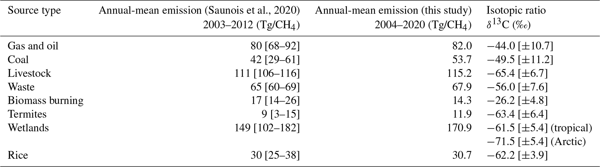
The post-2007 increase in atmospheric CH4 has been the focus of many studies and has been attributed to different plausible hypotheses associated with changes in various emissions sources and the OH sink (Turner et al., 2019). These studies have reached their conclusions using in situ mole fraction observations alone or in combination with other observations, e.g. in situ δ13C (Schaefer et al., 2016; Rice et al., 2016; Nisbet et al., 2016; Fujita et al., 2020; Lan et al., 2021; Basu et al., 2022; Oh et al., 2022), satellite observations (Worden et al., 2017; McNorton et al., 2018; Yin et al., 2021; Feng et al., 2022), or other trace gases, using a variety of analysis methods and computational models. Typical emissions sizes and uncertainties are indicated in Table 1, adapted from Saunois et al. (2020). Our approach is unique in that, for our δ13C inversion, we are solving for the δ13C isotopic source signature of a geographical region. From the isotopic source signature of a region, we can determine how the source balance within a particular region has shifted over time, e.g. larger or smaller contributions from pyrogenic and biogenic sources, and consequently gain understanding of the geographical shifts in the CH4 budget.
Table 1Global-mean emissions of different CH4 source types from bottom-up inventories (Saunois et al., 2020) and our a posteriori emissions estimates and the corresponding conventional isotope ratios' signatures (Sherwood et al., 2017). Uncertainties are shown as max–min values in square brackets.
Methane oxidation by the OH radical in the troposphere is responsible for 80 % of the total CH4 sink globally. Changes in OH may have played a role in recent changes in atmospheric CH4 (Rigby et al., 2017; Turner et al., 2017), but the magnitude of this influence is uncertain (its short atmospheric lifetime of <1 s makes direct measurement of global variability very difficult). Reducing values of OH effectively increases atmospheric CH4 and therefore has the same effect as increasing emissions of CH4. Chemical reactions responsible for removing CH4 from the atmosphere are faster for lighter isotopologues of CH4. This isotopic fractionation therefore leads to an atmosphere enriched in heavier isotopes relative to the globally emitted CH4. Lan et al. (2021) simulated CH4 and δ13C in a 3-D chemistry transport model covering the period 1984–2016 and found that changes in OH proposed by Turner et al. (2017) are not consistent with the trend of increasingly isotopically light δ13C observed in the atmospheric record. We explore the impact of reducing OH in a sensitivity study, taking into account a larger OH decrease during 2020 (Peng et al., 2022; Feng et al., 2023) that was associated with widespread reductions in nitrogen oxide emissions (Cooper et al., 2022).
Here, we calculate trends in regional CH4 emissions and isotopic δ13C source signatures across the world from 2004–2020 using in situ mole fraction and δ13C data and satellite column-averaged dry-air mole fraction data. This is achieved by using three sets of inversions: two maximum a posteriori inversions using ground-based data (solving separately for regional emissions and isotopic sources signatures) and an ensemble Kalman filter inversion using Greenhouse gases Observing SATellite (GOSAT) data (solving for regional CH4 emissions).
In the next section, we describe the data and methods we use to quantify changes in regional CH4 emissions and the corresponding regional stable isotope source signatures. In Sect. 3, we report our results of a posteriori regional CH4 fluxes and regional δ13C isotopic signatures, including analysis of sensitivity calculations that involve different assumptions about year-to-year changes in the OH sink. We conclude the paper in Sect. 4.
2.1 In situ and satellite remote measurements of atmospheric methane
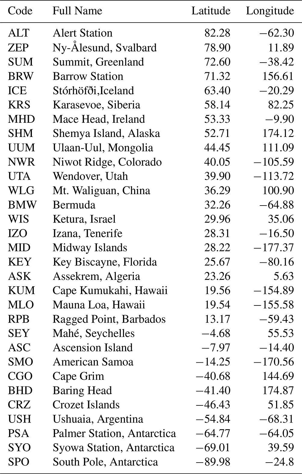
We use surface-level flask data as constraints on both regional CH4 emissions and the corresponding δ13 methane isotopic source signatures. The CH4 mole fraction data (version 2020-07; Dlugokencky et al., 2020) are taken from 31 National Oceanic and Atmosphere Administration – Global Monitoring Laboratory (NOAA-GML) sites around the world (Fig. 1). The data are monthly mean values that are averaged from discrete data as collected at each site; analysed at the NOAA – Earth System Research Laboratories (NOAA-ESRL) in Boulder, Colorado; and recorded according to the NOAA 2004A standard scale (Dlugokencky et al., 2005). Up to August 2019, the analysis was performed using gas chromatography (Steele et al., 1987; Dlugokencky et al., 1994, 2005), and since August 2019, cavity ring-down spectroscopy has been used (Dlugokencky et al., 2020). We also include data from a site in Siberia, Karasevoe (KRS), which is monitored by the National Institute for Environment Studies (NIES). This site was included to maximise geographical coverage of in situ data. The CH4 mole fraction measurements from this site are continuous, covering the period 2004–2020, and were made from 65 m height (Sasakawa et al., 2010). A scale factor of 0.997 is applied to the NIES data in order to bring them into line with the NOAA 2004A scale (Zhou et al., 2009). The site constitutes part of the Japan–Russia Siberia Tall Tower Inland Observation Network (JR-STATION).
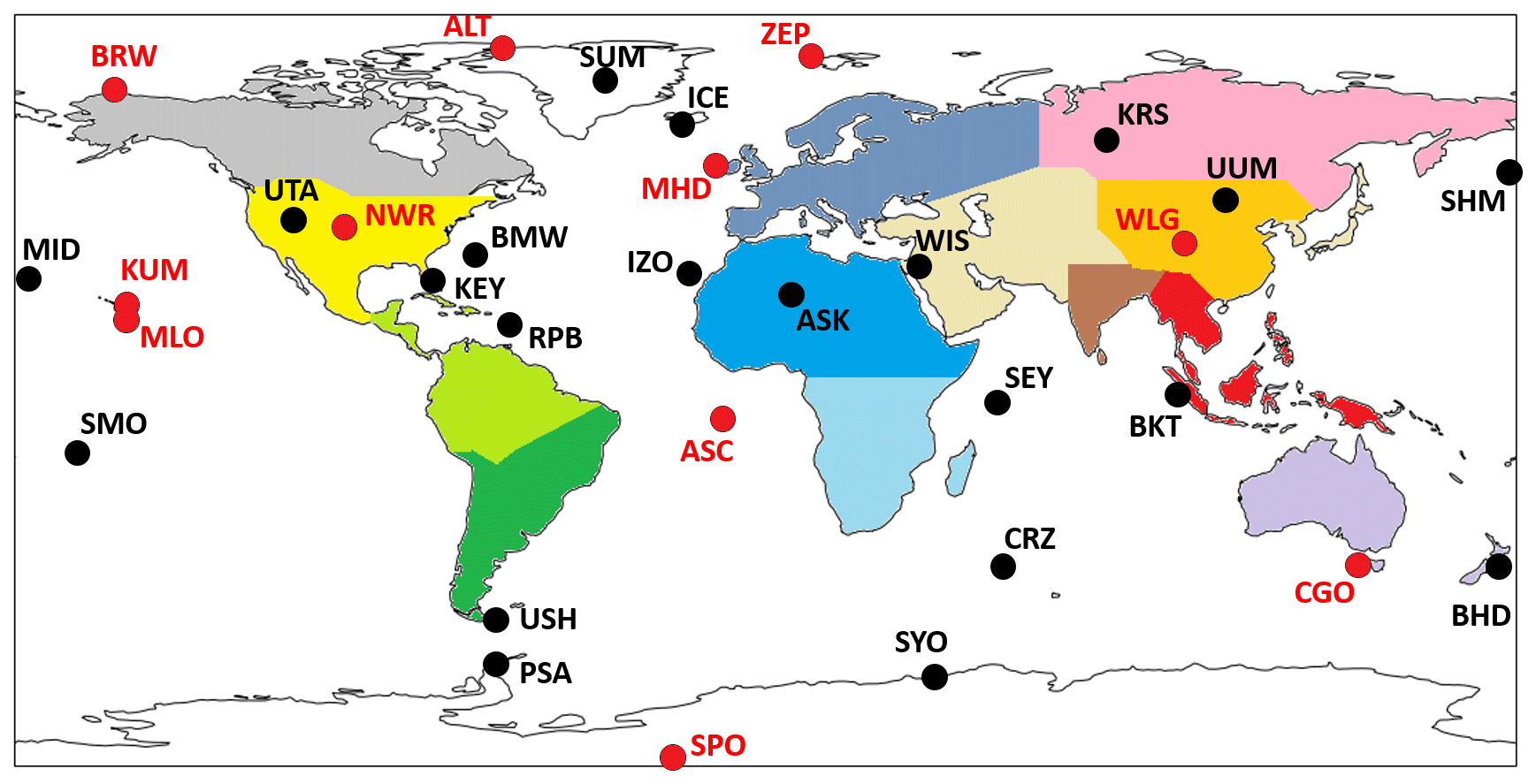
Figure 1Map showing regions that are optimised in the CH4 and δ13C inversions in different colours. Black dots and labels show the location of ground-based measurement sites that measure CH4 mole fraction. Red dots and labels indicate both CH4 mole fraction and δ13C measuring sites. Regions are named as follows: grey – North American boreal, yellow – North American temperate, light green – South American tropical, dark green – South American temperate, purple – Europe, blue – North Africa, light blue – southern Africa, pink – boreal Eurasia, orange – China, brown – India, peach – temperate Eurasia, red – tropical SE Asia, lilac – Oceania, white – oceans. Site identifiers are detailed in Table A2.
δ13C data are similarly monthly mean values that were calculated from discrete flask samples at NOAA network sites and reported on the international carbon isotope scale VPDB (Vienna Pee Dee Belemnite). Isotope ratio “delta” values represent the excess of a heavy, less abundant stable isotope (for δ13C values, carbon-13) over the light, most abundant stable isotope (carbon-12) in a sample when compared to a standard. These measurements are useful as they are indicative of the source of the CH4; biogenic sources are dominated by isotopically lighter signatures, and thermogenic sources are dominated by isotopically heavier signatures. For the NOAA network, isotopic analysis of δ13C was performed at the University of Colorado Institute of Arctic and Alpine Research Stable Isotope Laboratory (CU-INSTAAR). They follow an isotope ratio mass spectrometry approach (Miller, 2002; Vaughn et al., 2004). The geographical locations of in situ measurement sites are shown in Fig. 1. These sites are a subset of the entire NOAA network's capacity for measuring CH4 mole fractions. The sites included in the inversion (for both CH4 and δ13C) are those that cover the entire period of the inversion (2004–2020) without significant periods of measurement breaks to ensure a consistent interpretation of trends without consideration of possible biases introduced through the inclusion or exclusion of specific sites.
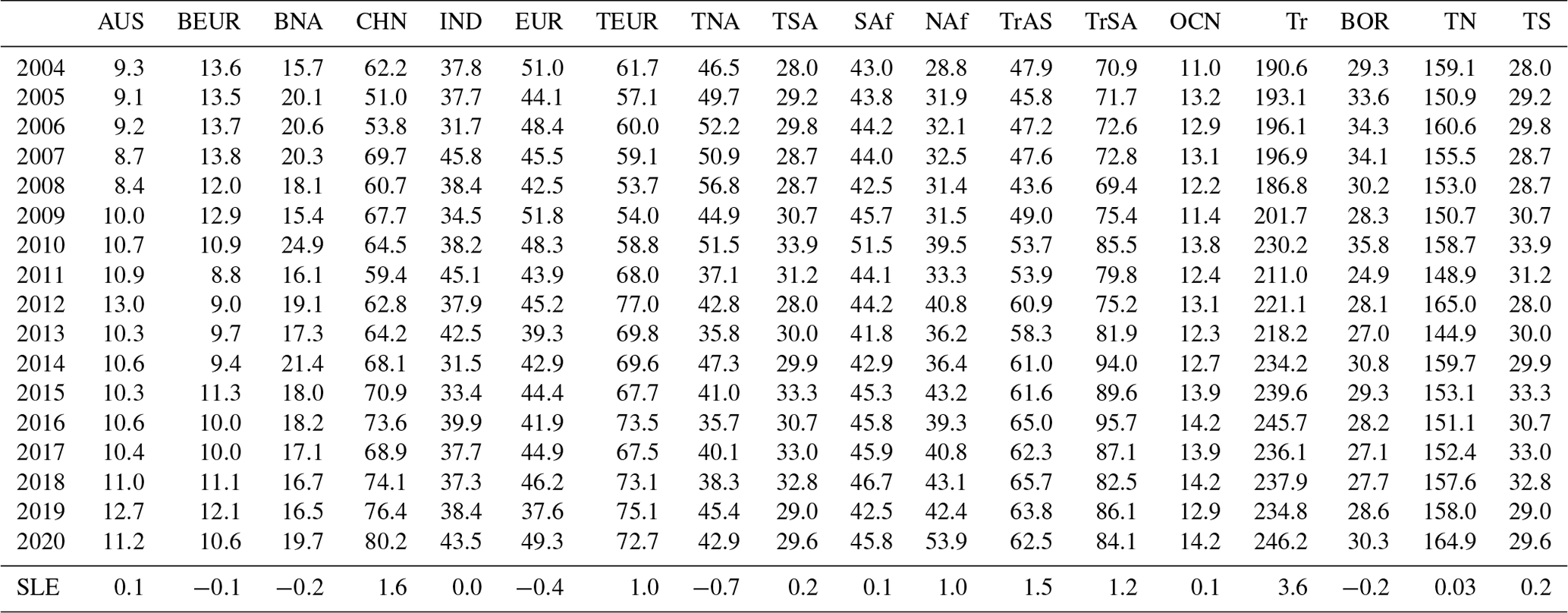
Table 2Annual regional-mean a posteriori CH4 emissions (Tg yr−1) from 2004 to 2020. Regions include Australia (AUS), boreal Eurasia (BEUR), boreal North America (BNA), China (CHN), India (IND), Europe (EUR), temperate Eurasia (TEUR), temperate North America (TNA), temperate South America (TSA), southern Africa (SAf), North Africa (NAf), tropical Asia (TrAS), tropical South America (TrSA), oceans (OCN), tropics (Tr), boreal (BOR), northern temperate (TN), and southern temperate (TS). The last row marked as SLE denotes the Siegel linear estimate of the linear trend in CH4 emissions (Tg yr−1 yr−1) over the 2004–2020 period.
We also estimate CH4 fluxes for 2010–2020 from the Japanese Greenhouse gases Observing SATellite (GOSAT) that was launched in 2009. GOSAT is in a sun-synchronous orbit with an equatorial local overpass time of 13:30. Since launch, it has provided continuous global observations of dry-air atmospheric-column-averaged CO2 (XCO2) and CH4 (XCH4), retrieved from shortwave infrared wavelengths that are most sensitive to changes in CH4 and CO2 in the lower troposphere (Parker et al., 2020). We use the latest (v9) proxy XCH4 : XCO2 retrievals that use spectral absorption features around the wavelength of 1.6 µm (Parker et al., 2020; Palmer et al., 2021) because of the smaller bias and better global coverage than those provided by the full physics retrievals. Analyses show the precision of a single proxy retrieval is about 0.72 %, with a global bias of 0.2 % (Parker et al., 2011, 2015, 2020). In our calculations, we assume a higher observation uncertainty of 1.2 % and deduct a globally uniform bias of 0.3 % to obtain better a posteriori agreement with the independent ground-based XCH4 data by the Total Carbon Column Observing Network (TCCON). These uncertainties are detailed in Feng et al. (2022). To anchor the constraints from the proxy XCH4 : XCO2 ratio (Fraser et al., 2014; Feng et al., 2017), we also assimilate the GLOBALVIEW CH4 and CO2 data (Schuldt et al., 2021), with assumed uncertainties of 0.5 ppm and 8 ppb for in situ measurements of CO2 and CH4, respectively. GLOBALVIEW constitutes a combination of CH4 data from ground-based data (both flask and continuous) and aircraft data from 54 different laboratories, combined and published by the NOAA-GML (Schuldt et al., 2021). Locations of the assimilated GLOBALVIEW CH4 (sub-)dataset are shown in Feng et al. (2022).
2.2 GEOS-Chem atmospheric chemistry and transport model
To relate CH4 emissions to atmospheric CH4 concentrations, we use v12.1 of the GEOS-Chem 3-D global chemical transport model (CTM) (Bey et al., 2001) at a horizontal resolution of 2∘ (latitude) by 2.5∘ (longitude) with 47 vertical levels from the surface to 80 km height using meteorological data from the MERRA-2 meteorological reanalyses (Gelaro et al., 2017) from the NASA Global Modeling and Assimilation Office (GMAO).
Our a priori emissions include (1) monthly EDGAR v6 anthropogenic emissions (Crippa et al., 2021) that account for emissions from oil and gas, coal, livestock, landfills, wastewater, rice, and other anthropogenic sources (including biofuel) from 2004 to 2018, after which we repeat 2018 emissions estimates; (2) monthly GFED-4 biomass burning emissions (version 4.1; Randerson et al., 2017); and (3) monthly v1.0 WetCHARTs wetland emissions (Bloom et al., 2017b). The Harvard–NASA Emissions COmponent (HEMCO) software within GEOS-Chem converts the emissions inventories at their native horizontal resolution to the GEOS-Chem 2∘ × 2.5∘ resolution. Beyond the end of the emissions inventory, emissions are repeated yearly in a priori simulation.
Table 1 shows the δ13C signatures for the source types included in our simulations. These are extracted as mean global values from Sherwood et al. (2017), which provide a database of global isotopic source signatures that are broken down into the same sectors as we employed in our simulations. However, individual source types show a wide range of source signatures, and this uncertainty is reflected in the assigned uncertainty given to the a priori source signatures in the inversion (Sect. 2.3). In the inversion, we differentiate between Arctic and tropical wetlands by applying a 10 ‰ isotopically lighter source signature to the Arctic source (Table 1) following Ganesan et al. (2018), who produced a global wetland source signature map based on published δ13C data. Recent work showed that atmospheric simulations that included this isotopic distinction between Arctic and tropical wetlands provided clearer support for rising microbial emissions being responsible for a large fraction of the increase in atmospheric CH4 since 2007 (Oh et al., 2022). In GEOS-Chem, we simulate isotopologues separately (i.e. for δ13C, 12CH4, and 13CH4) and then calculate δ13C values. The arithmetic underlying the conversion of isotope ratios to isotopologue emissions for input to the model is detailed in Appendix A.
We include the loss of atmospheric CH4 from reaction with chlorine, soil uptake, and oxidation by OH. We use monthly 3-D fields of OH, calculated using the full-chemistry version of GEOS-Chem, and monthly 3-D fields of atomic chlorine (Sherwen et al., 2016). Stratospheric loss frequency fields are determined using the NASA Global Modeling Initiative (GMI) stratospheric model (Duncan et al., 2007). Estimates of the microbial consumption of CH4 in soils are determined from Fung et al. (1991). The resulting atmospheric lifetime of CH4 against OH is 9.77 years. The corresponding lifetime for methyl chloroform is 5.41 years, which is consistent with atmospheric observation of methyl chloroform. This lifetime also compares well with a multi-model study (Voulgarakis et al., 2013; Morgenstern et al., 2017) that reported global-mean lifetimes of CH4 that range from 7.2–10.1 years. In our default model configuration, none of these loss processes include interannual variations.
To account for isotopic fractionation due to loss of CH4 in the troposphere and stratosphere, we use published kinetic isotope effect (KIE) values. These values are employed to scale the reaction rate constants used in the simulations for 12CH4 and 13CH4 (Table A1). The OH and Cl sinks are handled in the hard coding of the model, whereas the soil sink is handled as a negative emission in the HEMCO file. Therefore, for the soil sink, the KIE is directly applied as a scale factor in the HEMCO configuration file (Snover and Quay, 2000; Burkholder et al., 2019).
We created the initial conditions for atmospheric CH4 by first scaling a standard CH4 GEOS-Chem restart file (a file containing a default realistic distribution of CH4 across the atmosphere) to conditions nearly representative of the start of our analysis in January 2004. We then ran the model 60 times, repeating 2004 MERRA-2 meteorology and emissions (corresponding to approximately 6 e-folding lifetimes for CH4) to improve as far as possible the simulation of atmospheric gradients in CH4 under the initial conditions. We then ran a single-year inversion for 2004 to optimise the isotope ratios and CH4 concentrations relative to ground-based observations following the inverse method detailed below. The δ13C inversion used the regional emissions estimate provided by the posteriori from the CH4 inversion as a starting point, with sectoral emissions scaled as detailed in Appendix A. The output of this 2004 inversion is a final step in the creation of the initial conditions, which serve as a starting point for the longer inversion that we report here (2004–2020).
For all our calculations, we sample GEOS-Chem at the grid box and local time that correspond to the in situ and satellite remote sensing data. For the satellite data, we also apply scene-dependent averaging kernels to account for vertical structure. This approach allows us to directly compare the model with measurements. Regional trends are calculated by examining the grid boxes encompassed by a given region on the global grid.
2.3 Inverse methods
We use two inverse methods that reflect the volume and simplicity of the data being used. For in situ data we use the maximum a posteriori (MAP) inverse methods, and for the more voluminous satellite data we use an ensemble Kalman filter (EnKF). For brevity, we include only the essential details about either method and refer the reader to dedicated papers.
2.3.1 Maximum a posteriori
To infer regional a posteriori CH4 fluxes and regional δ13C emissions source signatures from the atmospheric measurements of CH4, we use the maximum a posteriori solution (MAP) inverse method (Rodgers, 2000). We solve for CH4 fluxes and δ13C emissions signatures from 14 geographical regions (Fig. 1). This method combines a priori knowledge and its uncertainty with the measurements and their uncertainties and has been used in a number of studies, e.g. Fraser et al. (2014) and McNorton et al. (2018).
The MAP solution and the associated a posteriori uncertainty are described as, respectively,
using the convention that lower-case and upper-case variables denote vectors and matrices, where x denotes the state vector that describes the estimated quantities, which in this study includes monthly CH4 fluxes and δ13C source signatures from regions across the world (Fig. 1). Subscripts “a” and “b” denote a posteriori and a priori CH4 fluxes, respectively, and superscripts “−1” and “T” denote matrix inverse and transpose operations, respectively. The measurement vector y includes CH4 mole fraction or δ13C data. The matrices B, A, and R denote a priori, a posteriori, and measurement error covariance matrices, respectively. B and R are diagonal matrices. For B we assume uncertainties of 50 % of the regional CH4 fluxes and 15 ‰ for the δ13C values, and for R we assume 10 ppb for the mole fraction data and 0.1 ‰ for the isotope data. These uncertainties were based on similar studies (Fraser et al., 2014; McNorton et al., 2016). We assume a model transport error of 12 ppb following Feng et al. (2022).
The Jacobian matrix H describes the sensitivity of the measurements to changes in the state vector, i.e. . For the CH4 mole fraction inversion, the Jacobian matrix describes the sensitivity of mole fractions in the model to changes in regional CH4 emissions. We construct the matrix using a series of GEOS-Chem model runs. We systematically let each individual emitting region (described by the state vector) emit for 1 month, while all other regions emit as normal. The individual regional source is then switched off (emissions set to zero), and the effect of this on the 3-D atmospheric distribution of CH4 mole fractions is recorded over the following 3 months. The result of this test is recorded at the grid boxes that correspond to the location of the measurement sites. The resulting mole fractions therefore describe the sensitivity of a particular measurement site to changes in a specific regional source up to 3 months after emission. This is repeated for every month within the inversion timescale and for every region described in the state vector.
For the δ13C inversions, the Jacobian matrix describes the sensitivity of modelled δ13C to changes in the regional isotopic source signatures. We construct the Jacobian as the difference between a control model calculation (using the CH4 a posteriori regional emissions and mean source signature values from Sherwood et al., 2017) and perturbed-source-signature model calculation for the whole study period (2004–2020). For the perturbed model calculation, we systematically perturb the isotopic source signature of each region (all of the sectors that are contained geographically within a region) isotopically heavier by 20 ‰ for the period 2004–2020. The difference in the δ13C value between the control and perturbed run at the location of each measurement site is then divided by the value of δ13C perturbation for the region's source signature to understand the effect of changing a region's source signature on the δ13C value recorded at each measurement site location.
The output from the inversion is improved estimates of regional CH4 fluxes and δ13C source signatures. The model simulates the global atmosphere on a 2∘ × 2.5∘ horizontal grid. The a posteriori regional CH4 fluxes and isotopic source signatures are applied to the grid boxes in the model which correspond to a given region in an a posteriori simulation.
2.3.2 Ensemble Kalman filter
We use an ensemble Kalman filter (EnKF) approach in performing the inversion using satellite data because we cannot easily evaluate the necessary matrix operations associated with an analytic inversion. Here we use an ensemble of flux perturbation pulses to represent uncertainty in our a priori estimate for regional monthly CH4 fluxes. We subsequently use a global chemistry transport model (i.e. the GEOS-Chem v12) to track the transport and chemistry processes of the tagged emissions pulses in the atmosphere in order to project their spreads to the observation space. With the ensemble of a priori flux perturbations and the simulated observation impacts, we use the ensemble transform Kalman filter (ETKF) algorithm to numerically estimate the a posteriori CH4 fluxes and the associated uncertainties by optimally comparing the model simulation with observations (see Feng et al., 2017, for more details). To reduce the computational costs, mainly from tracking tagged emissions pulses, we introduce a 4-month moving lag window for each assimilation step because any observation has limited ability to distinguish between the signals emitted long (>4 months) before from variations in the ambient background atmosphere (Feng et al., 2017). As a result, we are able to include a larger state vector, consisting of monthly scaling factors for 487 (476 land regions and 11 oceanic regions) regional CH4 (and CO2) pulse-like basis functions (Fig. S1 in Feng et al., 2022). We define these land sub-regions by dividing the 11 TransCom-3 (Gurney et al., 2002) land regions into 42 to 56 nearly equal sub-regions and use the 11 oceanic regions defined by the TransCom-3 experiment. Because of their smaller sizes, we have assumed a higher uncertainty percentage (60 %) for a priori emissions than the MAP approach described above. We also include spatial correlation with a correlation length of 500 km between the sub-regions.
2.4 Sensitivity of results to changes in assumed OH distributions
To examine the sensitivity of our results to changes in the magnitude of OH, we ran a single sensitivity run that is made up of two parts. First, we imposed a 0.5 % yr−1 uniform decrease on our 3-D OH field from 2004 to 2019, consistent with the 7 % reduction over 2003–2016 proposed by Turner et al. (2017). Second, we imposed a larger global-scale OH reduction of 1.5 % in 2020 based on recent studies (Miyazaki et al., 2021; Laughner et al., 2021) to describe a more abrupt change due to widespread reductions in nitrogen oxides (NOx) associated with closing down manufacturing during the first Covid-19 lockdown (Cooper et al., 2022). Newer studies have suggested that the OH reduction in 2020 was closer to 1 % (Peng et al., 2022; Feng et al., 2023), but these estimates are also subject to uncertainties. The purpose of this numerical experiment is to determine the sensitivity of a posteriori CH4 flux estimates to changes in assumed variations in OH and not to issue a proclamation about a time profile of OH that would simultaneously fit observed changes in CH4 and δ13C–CH4.
We use the Siegel linear non-parametric estimates (Siegel, 1982) to fit a line to our a posteriori CH4 emissions. This method is less sensitive to outliers, e.g. El Niño, that would otherwise compromise the linear-trend estimate (Palmer et al., 2021), and the resulting linear-trend estimate has lower variables than simpler methods. We find that Siegel trend estimates are similar to those estimated by the Theil–Sen estimator.
Here, we report a posteriori estimates for total CH4 emissions inferred from in situ and GOSAT data and then the corresponding a posteriori isotopic source signatures for δ13C. We draw comparisons with previous studies throughout this section.
A posteriori emissions estimates of total CH4
Figure 2 shows the annual-mean differences in regions between a priori emissions estimates and a posteriori emissions estimates for both ground-based (2004–2020) and GOSAT results (2009–2020). Absolute emissions values are plotted in Fig. 3 for completeness.
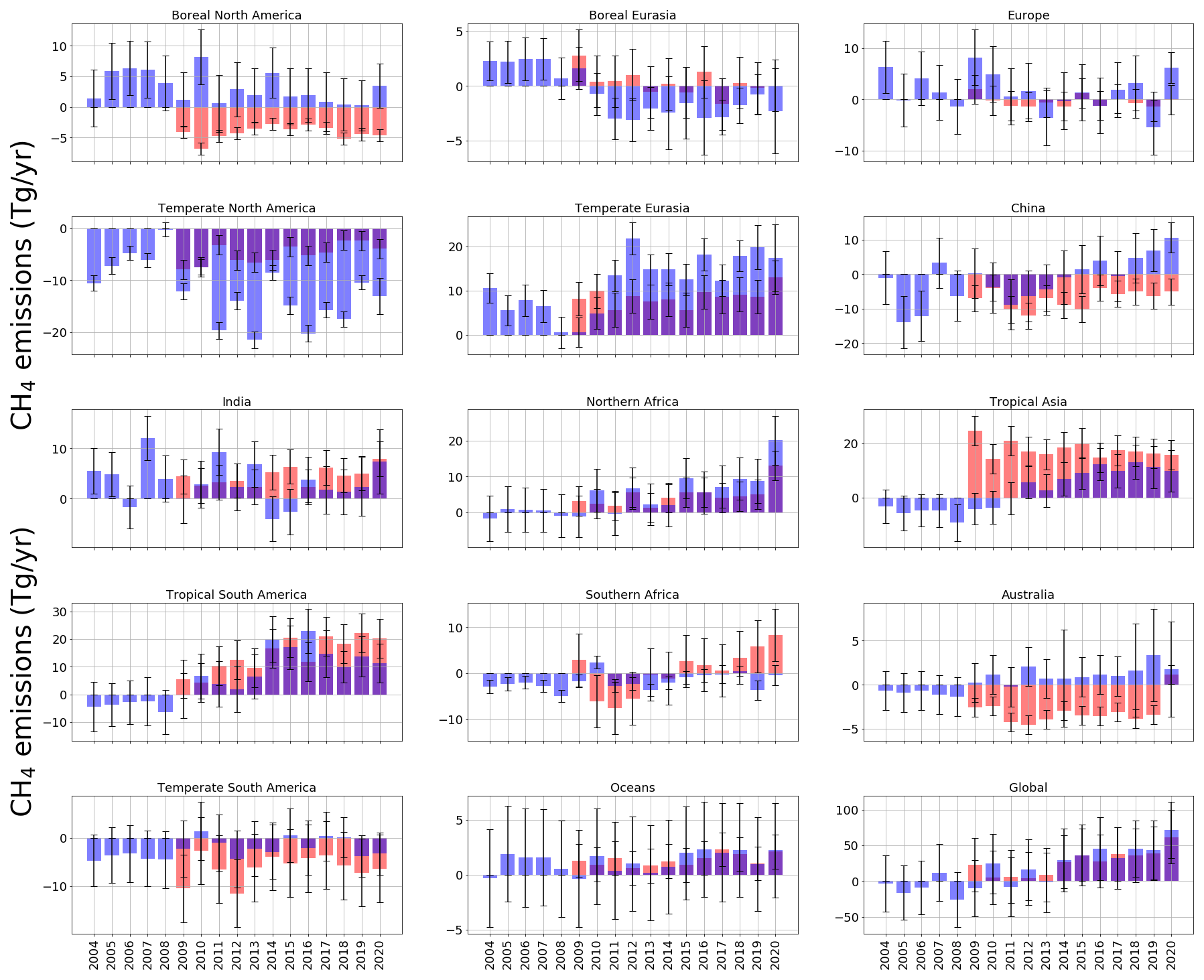
Figure 2Annual-mean CH4 a posteriori emissions estimates as a residual value relative to a priori values (Tg yr−1) from each of the inversion regions in latitudinal order (geographic coverage indicated in Fig. 1) for both ground-based and GOSAT inversion results. Uncertainties are indicated, as calculated from inversion calculations, with an a priori uncertainty of 50 % for the ground-based results and 60 % for the GOSAT results. The ground-based a posteriori is in blue; the GOSAT a posteriori is in red.
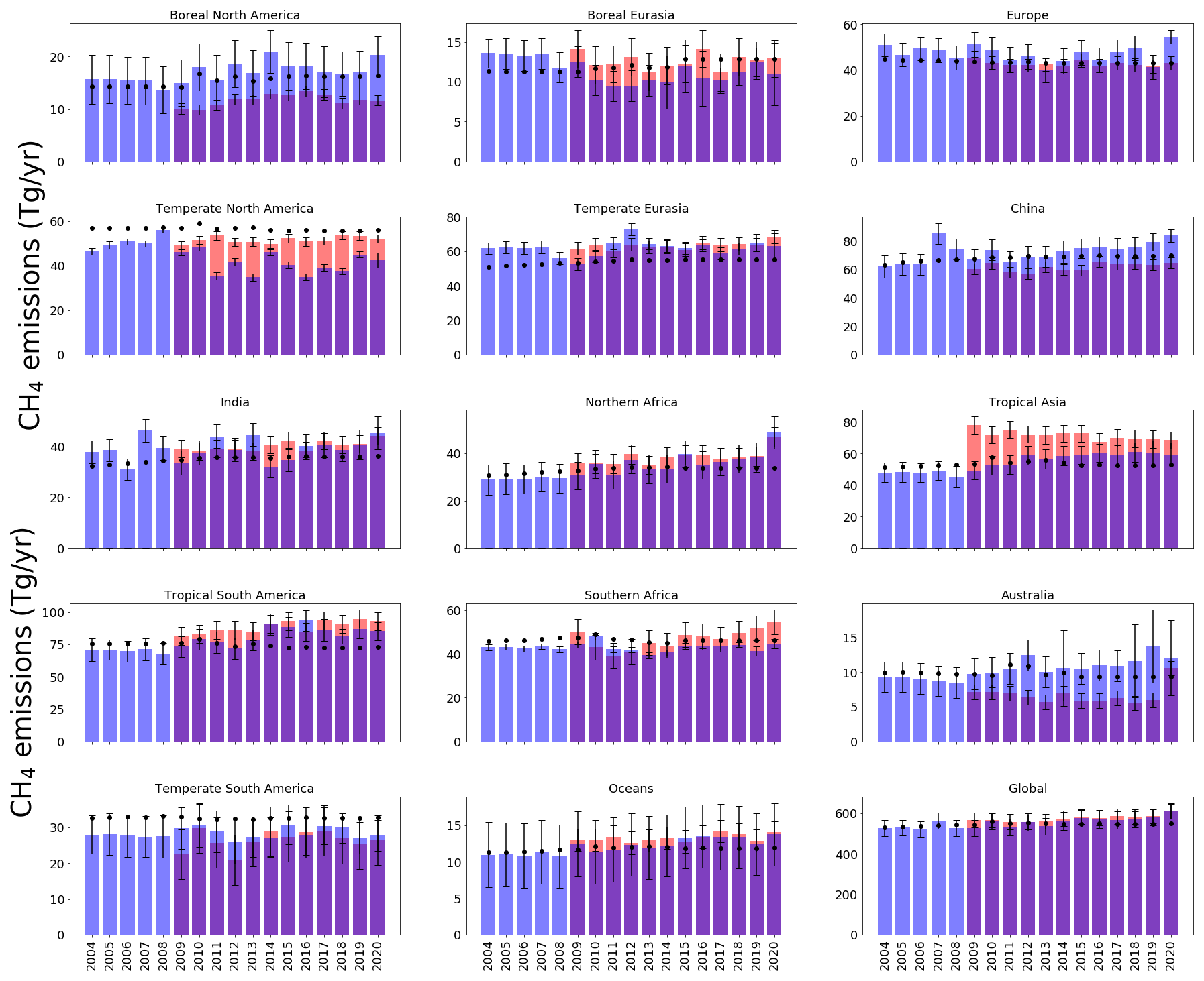
Figure 3A posteriori emissions estimates (Tg yr−1) inferred from ground-based in situ data (blue) and GOSAT data (red, with record starting in 2010) for the geographical regions shown in Fig. 1. A priori emissions estimates are denoted by black dots, and a posteriori uncertainties are denoted by whisker bars.
On a global scale, terrestrial a posteriori emissions inferred in situ and GOSAT data have progressively increased relative to a priori values since about 2014. The peak difference is in 2020, when we find increased emissions, relative to a priori emissions, of 68.5 ± 61.5 Tg yr−1 for the in situ inversion and of 61.5 ± 37.3 Tg yr−1 for the GOSAT inversion. Global ocean a posteriori CH4 emissions inferred from in situ and GOSAT data support a negative bias in the a priori emissions, which we do not discuss further.
As a zeroth-order check of our a posteriori emissions estimate of total CH4 (Fig. 4) we compare the published NOAA atmospheric growth rate of CH4 with our corresponding a posteriori atmospheric mole fractions. Generally, we find that the a posteriori values inferred from in situ and GOSAT data are consistent with the overall trend of the changes in the growth rate, with large year-to-year changes that we explain now in terms of regional emissions changes.
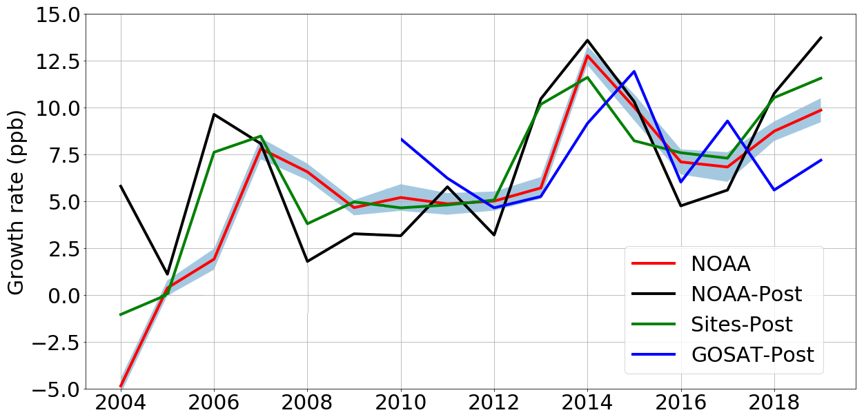
Figure 4A posteriori annual-mean atmospheric CH4 growth rate inferred from in situ (black line) and GOSAT data (blue line) compared with the equivalent data as published by the NOAA (red line, with uncertainty as surrounding blue field; Dlugokencky et al., 2020). The green line denotes the annual atmospheric growth rate determined using the in situ mole fraction data from the sites included in the inversion (“Sites-Post”). To calculate the atmospheric growth rates from model calculations (NOAA-Post and GOSAT-post), we compare the average global CH4 mole fraction in 1 year (the mean mole fraction of every grid box in every month of a year) with the mean value from the following year. The calculation is January–January in order to remove the effects of the seasonal cycle following the approach by the NOAA (Dlugokencky et al., 2020).
Changes in the global terrestrial emissions reflect changes from different geographical regions. Differences between a posteriori emissions estimates inferred from in situ and GOSAT data are partly due to differences in the geographic coverage of the datasets. Ground-based data have poorer geographic coverage, particularly over the tropics and the Southern Hemisphere, and satellite data are currently available at most once per day under cloud-free conditions. Using the in situ data, we find that the largest a posteriori emissions increases between 2004 and 2020, determined by the Siegel linear estimator, are over the tropics (3.6 Tg yr−1 yr−1; comprising North Africa, southern Africa, tropical South America, and tropical Asia), followed by China (1.6 Tg yr−1 yr−1). Smaller contributions (individually < 0.2 Tg yr−1) were made elsewhere.
Table 1 provides an overview of our annual-mean sector-based a posteriori emissions for 2004–2020. Generally, our values are close to the reported median values and within the range of values reported by Saunois et al. (2020).
Over the tropics, there is broad consistency between GOSAT and in situ data (Fig. 2) that highlights the negative bias in the a priori values over North Africa (bias of −8.6 Tg yr−1), tropical Asia (bias of −7.2 Tg yr−1), and tropical South America (bias of −11.63 Tg yr−1). The in situ and GOSAT data for China support a small, steady increase in emissions from 2009 to 2020 (1.0 Tg yr−1), with emissions inferred from the GOSAT data generally smaller than a priori values throughout the period (Fig. 2). Data over India have a small mean annual trend (0.33 Tg yr−1). In situ and GOSAT data are more consistent in sign (but not magnitude) at temperate latitudes (Fig. 2). A posteriori emissions from in situ and GOSAT data are generally lower by more than 12.0 and 5.6 Tg yr−1, respectively, over temperate North America and higher by more than 13.0 and 7.0 Tg yr−1, respectively, over temperate Eurasia, with the smallest discrepancies relative to the a priori values before 2009. A posteriori emissions from boreal regions appear to be larger than a priori values by 4.2 Tg yr−1 before 2009 (Fig. 2). After 2009, in situ data become progressively more consistent with the a priori over North America and are typically smaller than a priori values over Eurasia by ≃ 2.6 Tg yr−1. GOSAT appears to show the converse situation; after 2009, data are lower than a priori values by 4.4 Tg yr−1 over North America and comparable with a priori values over Eurasia. In the Southern Hemisphere, in situ data closely follow a priori values, as expected, since there are few places where data are collected. GOSAT data show a small but persistent increase in emissions with time over southern Africa (0.41 Tg yr−1), highlighting the negative bias in a priori emissions over Australia and over temperate South America.
We use the a posteriori error covariance matrix from our MAP inversion (A; Eq. 2) to determine our ability to independently estimate CH4 emissions from our geographical regions. Figure A1 shows no significant a posteriori correlations between neighbouring geographical regions in our state vector. This is consistent with the in situ data being able to independently estimate regional emissions estimates in our state vector.
Our a posteriori emissions estimates are broadly consistent with previous studies. For example, the increase in tropical emissions has been reported using GOSAT data or in situ data within a 3-D CTM inversion (McNorton et al., 2016; Fujita et al., 2020), which examined shorter time periods of 2003–2015 and 1995–2013, respectively. The increase over eastern Africa (which lies within our North Africa region) has been reported by several studies (Lunt et al., 2019, 2021; Pandey et al., 2021; Feng et al., 2022). Using GOSAT data, Sheng et al. (2021) reported that CH4 emissions from China increased by 0.36 Tg yr−1 from 2012 to 2017. Over the same time period, we estimate an increase of 0.64 and 0.50 Tg yr−1 inferred from in situ and GOSAT data, respectively.
Figure A2 shows observed CH4 time series at ground-based sites that we use to determine the corresponding GEOS-Chem a priori and a posteriori mole fractions. A priori values already show excellent agreement with observations (mean residual of 14.1 ppb and root-mean-square error, RMSE, of 18.3 ppb), but this is generally improved after the model is fitted to the in situ data, with smaller mean residuals (12.5 ppb) and RMSE (17.0 ppb). This is consistent with previous studies such as McNorton et al. (2018) that reported a posteriori RMSE values of 12.3 ppb. Figure A3 shows a posteriori CH4 mole fractions at NOAA sites that we do not include in the inversion. This provides an additional and independent test of our ability to describe atmospheric CH4 using a subset of NOAA data that we use in our inversion (Table A2). Generally, our a posteriori estimates agree with these independent data, but for some sites the model has difficulty reproducing the data, e.g. AMY (western South Korea), KZD (Kazakhstan), and SDZ (mainland China). This is because some sites are influenced by local sources that are not representative of the spatial scale of our transport model (≃ 50 000 km2). Similarly, we find agreement using a posteriori mole fractions using GOSAT data (Fig. A4; mean residual of 29.1 ppb and RMSE 35.1 ppb).
A posteriori source signatures of δ13C
Figure 5 shows source signatures of a posteriori regional δ13C emissions inferred from ground-based in situ data. We group our results into approximately 3-year bands, as a residual from the 2004–2007 mean value, to show how the regional isotopic source signatures change across the time series.
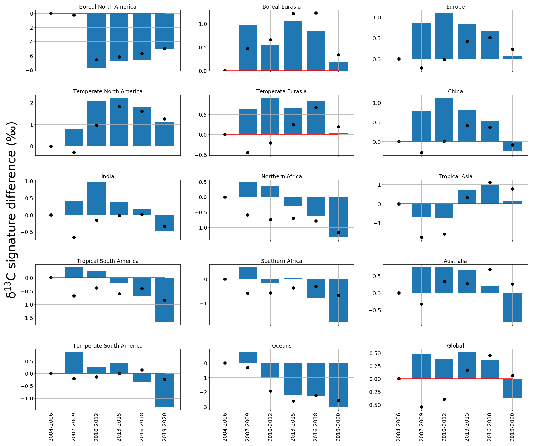
Figure 5Regional and global a posteriori δ13C emissions source signatures (‰) in 3-year groups (2004-06, 2007-09, 2010-12, 2013-15, 2016-18, 2019-20) as a residual from the 2004–2006 a posteriori regional emissions source signature value. The a priori equivalent is represented by black dots. The regions are those solved for in the CH4 and δ13C inversions and are indicated in Fig. 1.
Relative to a priori emissions (Fig. A5), a posteriori values from northern boreal regions (boreal North America and Eurasia) have isotopically lighter signatures (−62 ‰), consistent with a larger contribution from isotopically lighter biogenic emissions and/or a smaller contribution from isotopically heavier thermogenic or pyrogenic emissions (Fig. A5). Conversely, a posteriori values from regions such as temperate Eurasia, Australia, and southern Africa have isotopically heavier source signatures (approximately −40 ‰), suggesting a larger proportion of thermogenic or pyrogenic emissions and/or a smaller contribution from isotopically light biogenic emissions.
Figure 5 shows a general trend towards isotopically lighter regional source signatures of δ13C across the time series. Our analysis suggests that this trend has been ongoing since 2012 and is observed in all regions worldwide but is strongest (compared with a priori estimates) over tropical and Southern Hemisphere regions. For example, tropical South America and southern Africa are 1.2 ‰ and 0.9 ‰ isotopically lighter than a priori values for 2019 and 2020, respectively.
Our analysis also highlights the period 2007–2012, when regional source signatures, particularly in Northern Hemisphere regions, become isotopically heavier compared with a priori source signatures (by 1.0 ‰ between 2007–2009, by 0.8 ‰ between 2010–2012, and by 0.3 ‰ between 2013–2015). After 2012, regional source signatures of δ13C generally become isotopically lighter. This result suggests that 2012 was a period when there was a change in the balance of global sources that determine changes in atmospheric CH4. These isotopic shifts in 2008 and 2012 are noted by Nisbet et al. (2016), who used a box model and examine data from sites measured by the NOAA and Royal Holloway, University of London (RHUL). They found that changes in removal rates could not explain these anomalies so that these events were attributed to changing emissions. We find that China experiences a weaker shift in 2012 to an isotopically lighter (∼ 0.1 ‰) δ13C source signature compared to a priori values (Fig. 5) and compared to other temperate regions. This suggests that heavier isotopic source signatures (such as coal mines) make a larger contribution to this region.
Unlike the a posteriori total CH4 emissions estimates, we find significant a posteriori correlations between neighbouring regions for δ13C source signatures (Fig. A6). For example, there is a correlation of 0.95 between estimates for southern Africa and temperate South America, so these cannot be considered to be independent estimates. This result aligns with Basu et al. (2022), who used CH4 mole fraction and δ13C measurements to determine that tropical biogenic sources are driving CH4 growth. They acknowledged that measurement coverage limited conclusions based exclusively on isotope ratio measurements. Nevertheless, they found a clear trend of stronger emissions of isotopically lighter CH4, indicative of an increased role for biogenic emissions in the global source makeup.
We find that a posteriori regional δ13C source signatures result in a time series of δ13C that is more consistent with observations than a priori values (Fig. A7), as expected. This particularly affects the period 2008–2018, when a priori emissions source signatures are significantly isotopically lighter. Our a posteriori source signatures result in a mean observation—model residual and RMSE of 0.11 ‰ and 0.14 ‰, respectively. These are smaller than those corresponding to a priori values for the observation—model residual (0.37 ‰) and RMSE (0.41 ‰). Our comparison is consistent with McNorton et al. (2018) (RMSE of 0.1 ‰) and Fujita et al. (2020) (RMSE of 0.08–0.25 ‰).
Sensitivity to assumptions about OH
Figure 6 shows the result of our sensitivity test, which assumes a 0.5 % yr−1 uniform decrease in our 3-D OH field from 2004 to 2019, followed by a more abrupt decrease of −1.5 % in 2020, to describe the widespread reduction in nitrogen oxide emissions. This is an idealised sensitivity test that is inconsistent with global-scale constraints on estimates of the global-mean atmospheric growth of atmospheric CH4; i.e. most of the observed global growth in atmospheric CH4 can be explained by the changes in OH. Nevertheless this test provides us with some idea of the robustness of our results against changes in OH.
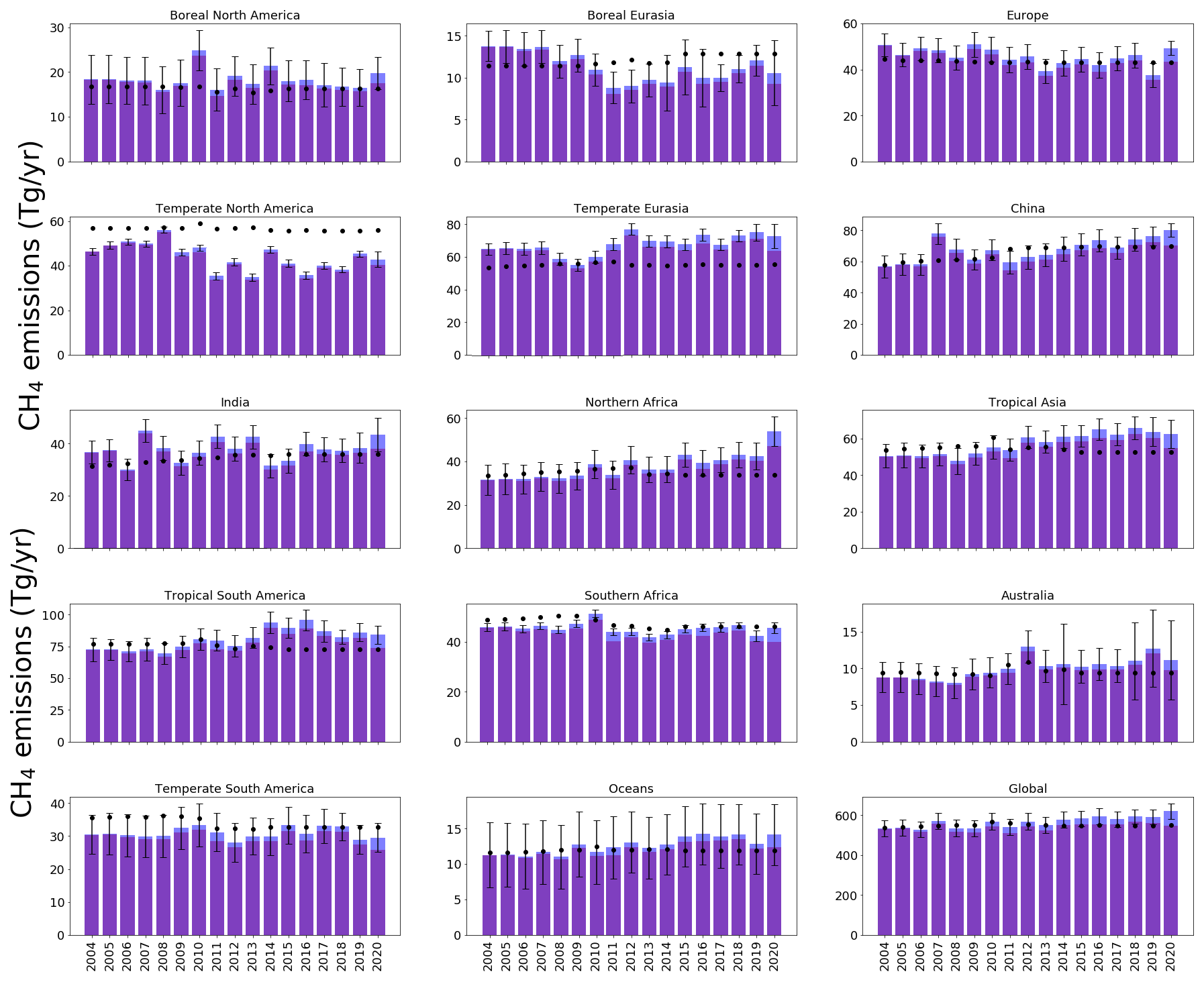
Figure 6Annual-mean CH4 emissions (Tg yr−1) for each region of the inversion (indicated in Fig. 1) inferred from the ground-based data (dark blue) and the emissions estimates determined by reduced OH values (described in the text, shown in red). A priori regional emissions estimates are indicated by black dots. Regional uncertainties for the a posteriori emissions are indicated.
We find that this alternative assumption about OH does not significantly affect our results until much later in the time series (2017–2019), reflecting our large a posteriori uncertainties. We find a similar quality of fit of the a posteriori model to the data with or without considering the OH trend (not shown). This does not preclude a role for changes in OH, but the concurrent a posteriori shifts in CH4 emissions and regional isotopic source signatures of δ13C are consistent with decreasing OH playing a smaller role than increasing emissions with isotopically light δ13C source signatures in determining observed changes in atmospheric CH4 (Lan et al., 2021).
The larger, abrupt change in 2020 results in a marked reduction (approximately 6 %, ∼ 40 Tg yr−1) in the emissions necessary to explain the increase in atmospheric CH4. There is still debate about the impact of a posteriori CH4 methane emissions. Peng et al. (2022) used in situ data and concluded that the increase in atmospheric CH4 in 2020 could be attributed approximately equally to a decrease in OH and an increase in OH. Analysis of GOSAT suggests that increased emissions play a larger role (Qu et al., 2022; Feng et al., 2023).
We estimated regional CH4 emissions and δ13C source signatures for the period 2004–2020, inclusively, by fitting the GEOS-Chem 3-D atmospheric chemistry transport model to surface mole fraction data (Fig. 1) and GOSAT atmospheric column data (2010–2020) using Bayesian inverse methods. We used surface sites for which we had complete monthly coverage over most of the study period (Table A2). Collectively, our results indicate that the post-2007 increases in CH4 emissions are best explained by a progressive latitudinal shift in emissions from the northern mid-latitudes to tropical latitudes. A posteriori CH4 emissions estimates inferred from the ground-based and GOSAT data show larger tropical emissions, particularly over North Africa, tropical Asia, and tropical South America as well as over China and at the same time as mid-latitudinal emissions proportions decrease. Source signature estimates inferred from the δ13C measurements (Fig. 1) over the same time period indicate that the latitudinal shift in CH4 emissions is due to a larger proportion of sources with a lighter atmospheric δ13C signature (e.g. biogenic source such as wetlands) and/or a smaller proportion of sources with a heavier atmospheric δ13C signature (e.g. thermogenic or pyrogenic sources). Our results are broadly consistent with previous studies that focus on shorter contributing periods (McNorton et al., 2018; Nisbet et al., 2019; Fujita et al., 2020; Yin et al., 2021; Lan et al., 2021; Basu et al., 2022), providing confidence in our model assumptions and data selection. We find that our main results are robust against assuming a 0.5 % yr−1 OH decrease from 2004 to 2019, consistent with Turner et al. (2017), followed by an abrupt 1.5 % OH drop in 2020 that reflects the widespread decrease in nitrogen oxide emissions from shutting down manufacturing during the first Covid-19 lockdown. This is an idealised sensitivity test but nevertheless provides us with some idea of the robustness of our results against changes in OH. A more detailed discussion of the role of OH in 2020 is discussed elsewhere (Qu et al., 2022; Peng et al., 2022; Feng et al., 2023).
Sparse geographic coverage of ground-based data results in larger uncertainties for regional emissions estimates that are informed by fewer data, i.e. high and low latitudes in both hemispheres. For CH4, this deficiency can be partly addressed using the satellite data, but isotope ratios cannot usefully be retrieved from Earth observation satellite instruments. We use only three measurement sites for δ13C in the Southern Hemisphere, which have a continuous record over the period of study. A consequence of this data sparsity is strong correlations between source signatures from neighbouring regions (Fig. A6). We assume mean sectoral δ13C source signatures from Sherwood et al. (2017). These values are highly uncertain, as different sectors produce a range of possible δ13C values, and there are significant overlaps between recorded source signatures (Douglas et al., 2017), but the values chosen represent our current best knowledge of mean values. These data have greater value when they are used in a broader context with other data, as we describe in this study. We have used satellite observations to help identify that large-scale emissions change over regions that coincide with wetlands.
Collectively, empirical evidence, including in situ and GOSAT observation of CH4 and in situ δ13C data, points to an increasing biogenic source originating from the tropics. While we cannot definitively attribute these changes to increasing wetland emissions, there is sufficient contextual evidence, building on previous studies, to suggest that wetlands have played a significant role in recent growth of atmospheric CH4. First, large changes in OH that would be needed to explain this atmospheric growth are inconsistent with increasingly isotopically light δ13C observations in the atmospheric record (Lan et al., 2021). Second, we know from in situ data the broad geographical regions responsible for increasing CH4 emissions and isotopically lighter δ13C source signature, where the seasonal cycles are consistent with biogenic emissions peaking outside the burning season. Third, GOSAT provides us with additional information about the geographical distribution of CH4 emissions; tropical emissions hotspots are colocated with known wetland regions (Lunt et al., 2019, 2021; Pandey et al., 2021; Wilson et al., 2021; Feng et al., 2022, 2023). Finally, we also have evidence from other satellite data, e.g. hydrology, that helps explain the growth of wetland emissions in the last decade (Lunt et al., 2019; Feng et al., 2022). Greater confidence in source attribution of changes in atmospheric CH4 may come from collecting and interpreting δD and multiply substituted “clumped” isotopes (Douglas et al., 2017; Chung and Arnold, 2021), alongside δ13C. This needs to be accompanied by field measurements of these isotope ratios to improve delineation between different sectors.
The evidence presented here is consistent with a growing body of work that points to a substantial increase in biogenic CH4 emissions from the tropics. This increase will likely have major implications for achieving the goals of the Paris Agreement (Nisbet et al., 2019). Nature does not care about the origin of atmospheric CH4 so that increasing biogenic emissions will require larger emissions reductions from anthropogenic sectors, placing additional pressure on citizens to reduce their carbon footprints.
To simulate the atmospheric isotope ratio δ13C, the isotopologues 12CH4 and 13CH4 are considered separately in the model. To calculate the specific sectoral isotopologue emissions we use the emissions calculated from the CH4 mole fraction simulation and the isotope ratios defined in Table 2. We consider the isotope 13C relative to all isotopes in the sample (designated hereafter as 13x) using
where is calculated from the δ13C reported on the international carbon isotope scale VPDB (Vienna Pee Dee Belemnite). This is the proportional molar abundance of the isotopologues containing 13C (dominated by 13CH4) relative to the isotopologues containing 12C (dominated by 12CH4). This value has to be adjusted before being applied in GEOS-Chem to convert from isotope ratio values to kilogram values used by emissions inventories:
where SF13 is the scale factor applied to each emissions type for the 13CH4 simulation, M13 is the molecular weight of 13CH4 (17.035 g mol−1), and Mtot is the molecular weight of CH4 (16.04 g mol−1).
For the 12CH4 counterpart to 13CH4, we use a similar approach. The ratio of 12C to all isotopes in the sample (designated as 12x) is given by
This is similarly adjusted from molar to mass ratio; SF12 is the scale factor for each emissions type in the 12CH4 simulations:
where M12 is the molecular weight of 12CH4 (16.03 g mol−1). Since 13C and 12C are the only stable carbon isotopes of CH4, 13x and 12x should sum to 1.
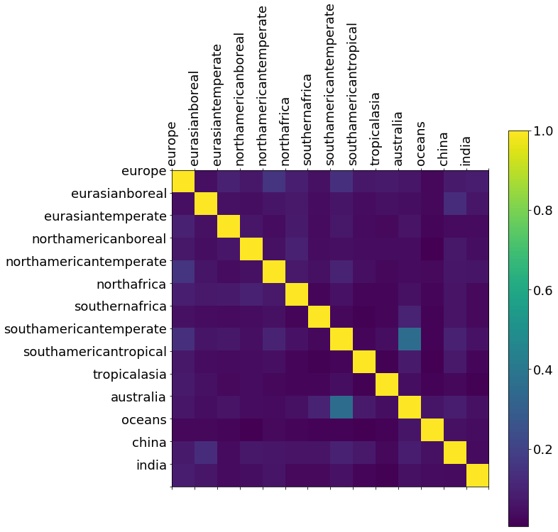
Figure A1A posteriori correlations between CH4 emissions from geographical regions inferred from ground-based CH4 mole fraction data. These correlations are determined by normalising the diagonal elements of the a posteriori error covariance matrix (Eq. 2).
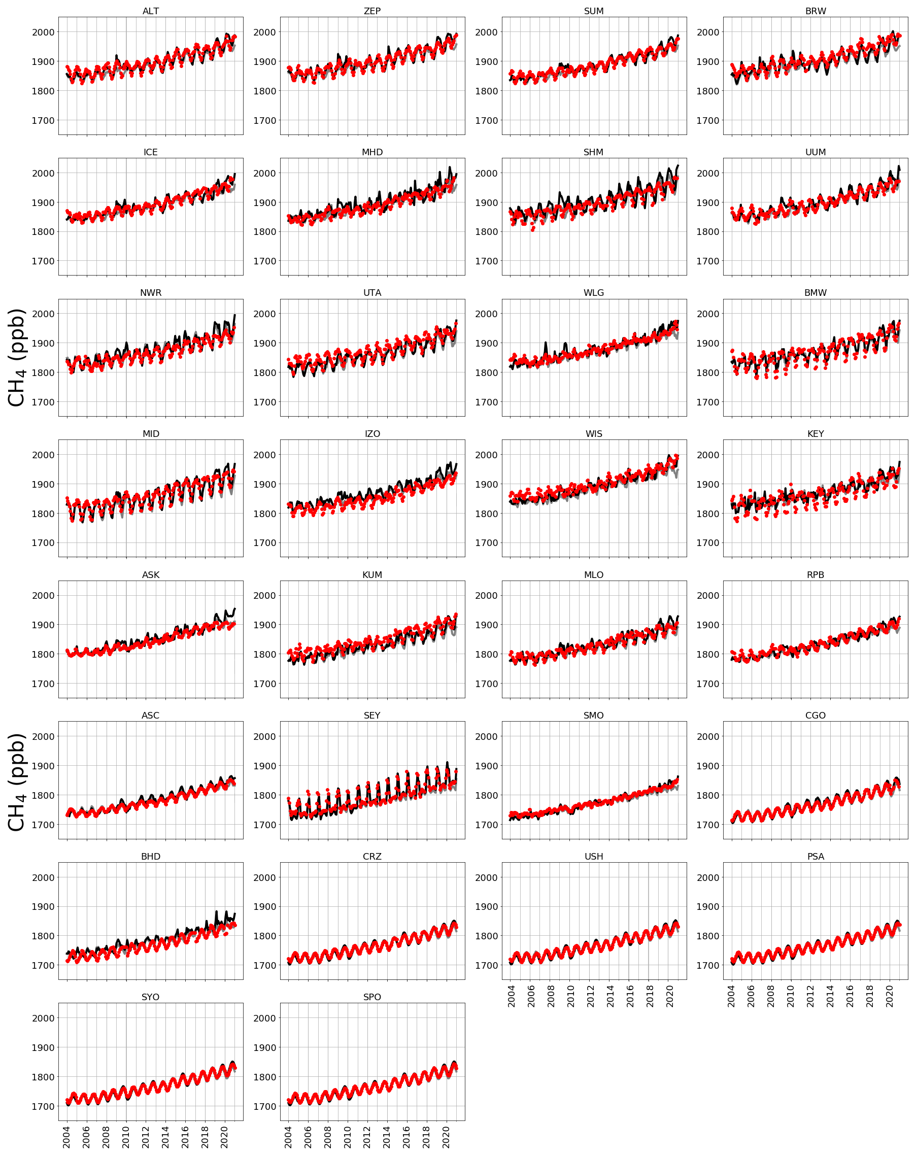
Figure A2Observed (red), a priori (grey), and a posteriori (black) model atmospheric mole fractions at a series of NOAA sites (subplot titles denote site codes; Table A2) covering a range of latitudes.
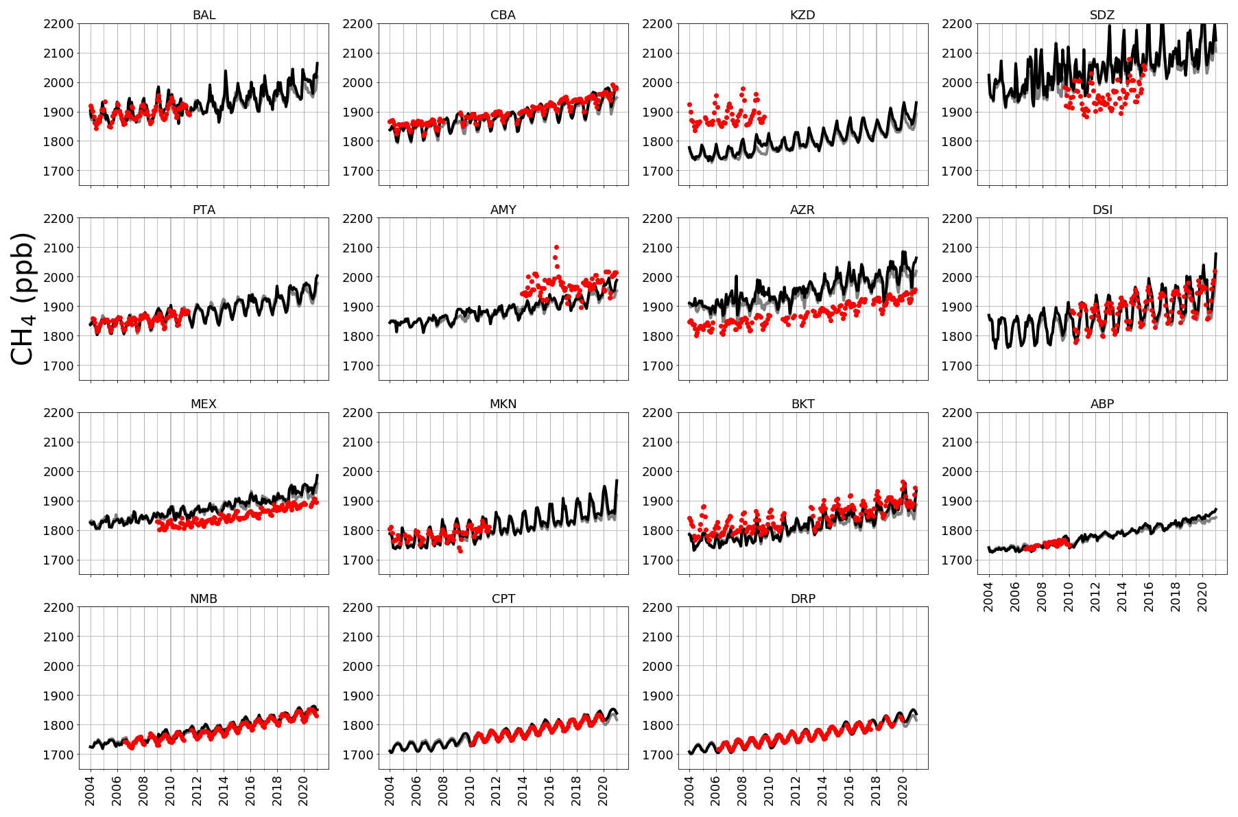
Figure A3A posteriori (black) monthly estimates of atmospheric CH4 simulated at NOAA sites across latitudes. Red indicates monthly mean CH4 data from the NOAA network sites indicated. These sites were not included in the CH4 inversion but are shown here to provide independent validation of a posteriori emissions. The sites included are Baltic Sea, Poland (55.35∘ N, 17.22∘ E); Cold Bay, Alaska (55.21∘ N, 162.72∘ W); Sary Taukum, Kazahkstan (44.08∘ N, 76.87∘ E); Shangdianzi, China (44.65∘ N, 117.12∘ E); Point Arena, USA (38.95∘ N, 123.74∘ W); Anmyeon-do, Republic of Korea (36.54∘ N, 126.38∘ E); Terceira Island, Azores (38.77∘ N, 27.37∘ W); Dongsha Island, Taiwan (20.70∘ N, 116.73∘ E); High Altitude Global Climate Observation Center, Mexico (18.98∘ N, 97.31∘ W); Mt. Kenya, Kenya (0.06∘ S, 37.29∘ E); Bukit Kototabang, Indonesia (0.20∘ S, 100.31∘ E); Arembepe, Brazil (12.77∘ S, 38.17∘ W); Gobabeb, Namibia (23.58∘ S, 15.03∘ E); Cape Point, South Africa (34.35∘ S, 18.49∘ E); and Drake Passage (59.00∘ S, 64.69∘ W).
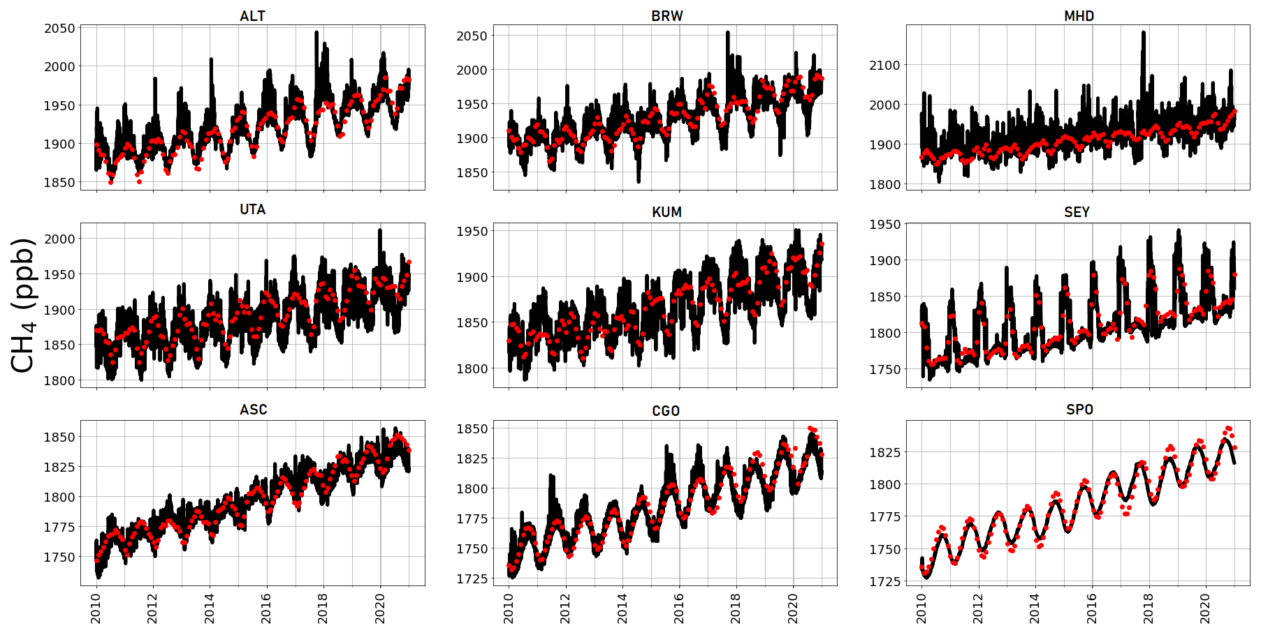
Figure A4Observed (red) and 3-hourly surface a posteriori CH4 values inferred from GOSAT data (black) at the location of a number of NOAA sites (Table A2) from 2010–2020.
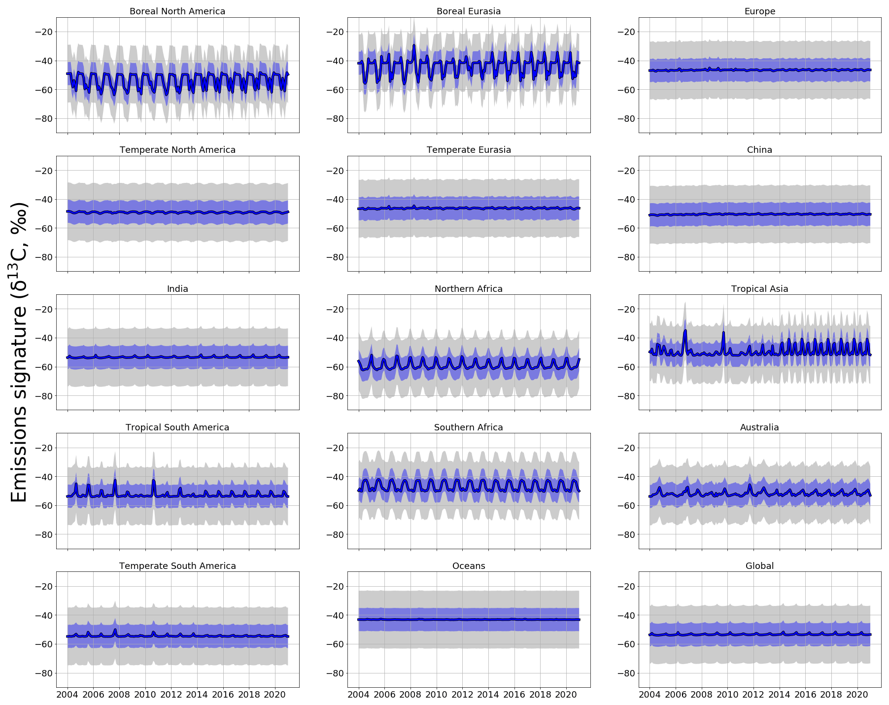
Figure A5Monthly a priori (grey) and a posteriori (blue) regional δ13C source signatures (‰). Values are produced using ground-based in situ δ13C data. Uncertainties in source signatures are indicated as shaded envelopes, with a priori uncertainties of 15 ‰.
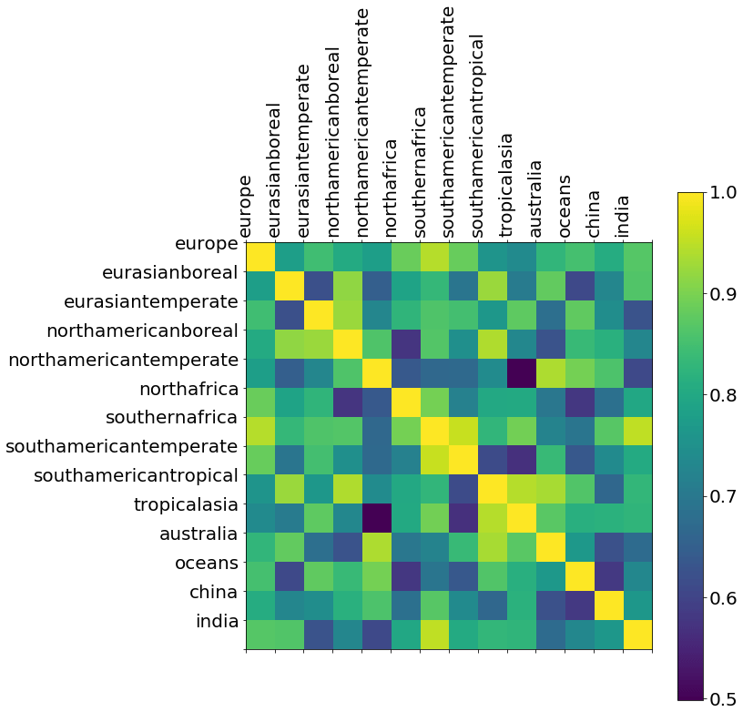
Figure A6A posteriori correlations between δ13C source signatures from geographical regions inferred from ground-based δ13C data. These correlations are determined by normalising the diagonal elements of the a posteriori error covariance matrix (Eq. 2).
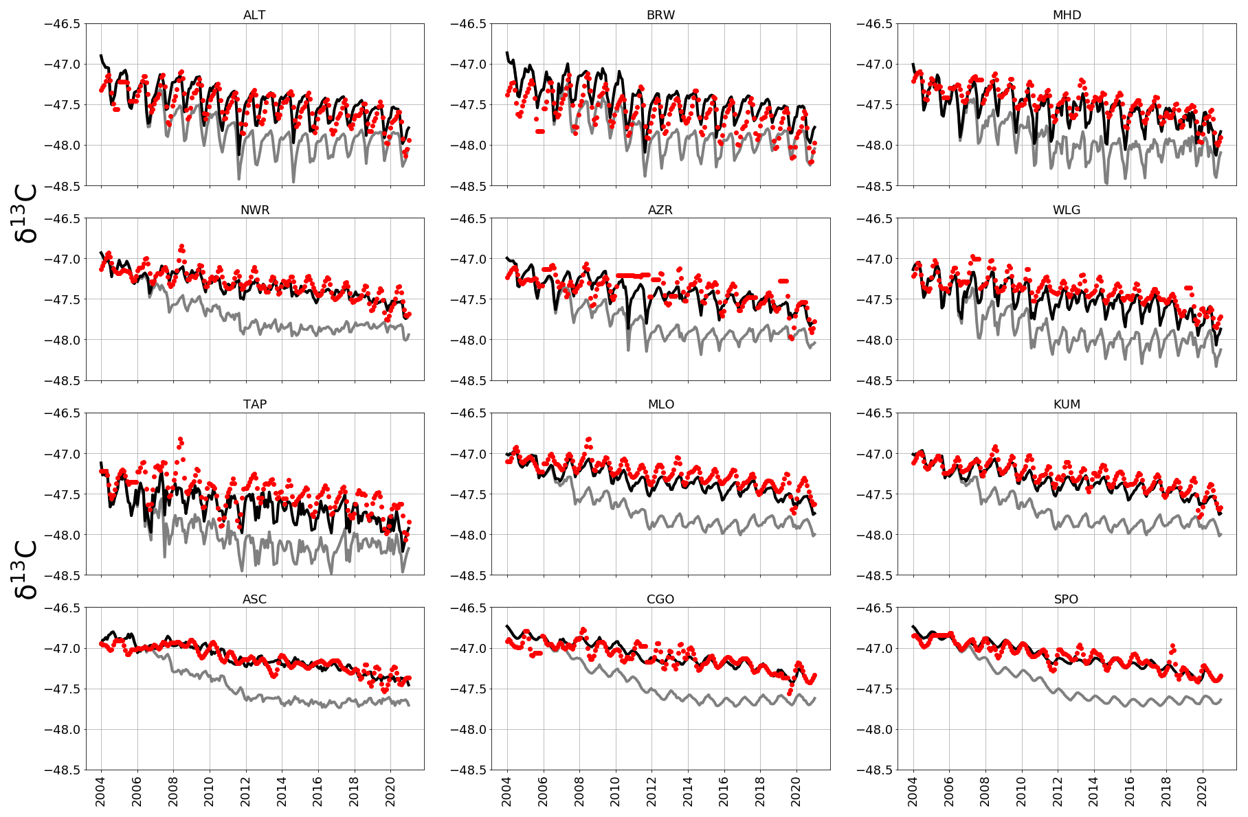
Figure A7A priori (grey) and a posteriori (black) monthly estimates of atmospheric δ13C simulated at NOAA sites across latitudes (site codes listed in Table A2). Red indicates monthly mean δ13C data from CU-INSTAAR for the respective sites.
Table A1Kinetic isotope effects (KIEs) for different isotopologues reacting with the three main sinks of CH4 (OH, Cl, soil) at 298 K. A KIE indicates relative reaction rate compared with 12CH4, the reaction rate constant is applied to the OH and Cl sinks and is dependent on temperature (T), and the scaling factor is applied to the soil sink at each time step (handled as a negative emission).
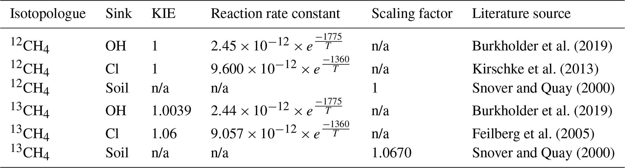
n/a – not applicable
Table A2Sites that are included in the in situ inversions. All sites are part of the NOAA network except for KRS, which is part of the JR-STATION network, monitored by NIES Japan.
The community-led GEOS-Chem model of atmospheric chemistry is maintained centrally by Harvard University (https://geoschem.github.io/, Bey et al., 2001) and is available on request. The ensemble Kalman filter code is publicly available as PyOSSE (https://www.nceo.ac.uk/data-tools/atmospheric-tools/, Feng et al., 2009).
All the data and materials used in this study are freely available. The NOAA-GML and CU-INSTAAR ground-based CH4 and δ13C data are available from the NOAA GML FTP server (https://gml.noaa.gov/dv/data, last access: 24 July 2023, https://doi.org/10.15138/VNCZ-M766, Dlugokencky et al., 2020), subject to their fair-use policies. Data from the JR-STATION network were provided with the cooperation of NIES Japan. The University of Leicester GOSAT Proxy v9.0 XCH4 data are available from the Centre for Environmental Data Analysis data repository at https://doi.org/10.5285/18ef8247f52a4cb6a14013f8235cc1eb (Parker and Boesch, 2020) and from the Copernicus Climate Data Store. EDGAR data are available at https://edgar.jrc.ec.europa.eu/ (Crippa et al., 2021), GFED-4 data are available at https://www.globalfiredata.org/data.html (last access: 24 July 2023, https://doi.org/10.3334/ORNLDAAC/1293, Randerson et al., 2017), and WetCHARTs data are available at https://doi.org/10.3334/ORNLDAAC/1502 (Bloom et al., 2017b).
AD led the data analysis with contributions from PIP and LF. AD and PIP led the writing of the paper with contributions from LF and TA. XL, SM, RP, and HM provided data.
The contact author has declared that none of the authors has any competing interests.
Publisher's note: Copernicus Publications remains neutral with regard to jurisdictional claims in published maps and institutional affiliations.
We thank the NOAA-ESRL and CU-INSTAAR for providing CH4 and δ13C data. We thank the Japanese National Institute for Environmental Studies and the Ministry of Environment for the GOSAT data and their continuous support as part of the Joint Research Agreements at the universities of Edinburgh and Leicester. We also thank the GEOS-Chem community, particularly the team at Harvard, who help maintain the GEOS-Chem model, and the NASA Global Modeling and Assimilation Office (GMAO), who provide the MERRA-2 data product.
Alice Drinkwater is supported by the University of Edinburgh's E3 Doctoral Training Partnership, funded by the Natural Environment Research Council (NERC), and by the National Physical Laboratory, UK. Paul I. Palmer, Liang Feng, and Robert Parker are supported by the National Centre for Earth Observation funded by NERC (grant nos. NE/R016518/1 and NE/N018079/1) and by the Copernicus Climate Change Service (C3S2_312a_Lot2).
This paper was edited by Frank Dentener and Patrick Jöckel and reviewed by four anonymous referees.
Allen, R. J., Zhao, X., Randles, C. A., Kramer, R. J., Samset, B. H., and Smith, C. J.: Surface warming and wetting due to methane's long-wave radiative effects muted by short-wave absorption, Nat. Geosci., 16, 314–320, 2023. a
Basu, S., Lan, X., Dlugokencky, E., Michel, S., Schwietzke, S., Miller, J. B., Bruhwiler, L., Oh, Y., Tans, P. P., Apadula, F., Gatti, L. V., Jordan, A., Necki, J., Sasakawa, M., Morimoto, S., Di Iorio, T., Lee, H., Arduini, J., and Manca, G.: Estimating emissions of methane consistent with atmospheric measurements of methane and δ13C of methane, Atmos. Chem. Phys., 22, 15351–15377, https://doi.org/10.5194/acp-22-15351-2022, 2022. a, b, c
Bey, I., Jacob, D. J., Yantosca, R. M., Logan, J. A., Field, B. D., Fiore, A. M., Li, Q., Liu, H. Y., Mickley, L. J., and Schultz, M. G.: Global modeling of tropospheric chemistry with assimilated meteorology: Model description and evaluation, J. Geophys. Res.-Atmos., 106, 23073–23095, https://doi.org/10.1029/2001JD000807, 2001. a, b
Bloom, A. A., Bowman, K. W., Lee, M., Turner, A. J., Schroeder, R., Worden, J. R., Weidner, R., McDonald, K. C., and Jacob, D. J.: A global wetland methane emissions and uncertainty dataset for atmospheric chemical transport models (WetCHARTs version 1.0), Geosci. Model Dev., 10, 2141–2156, https://doi.org/10.5194/gmd-10-2141-2017, 2017a. a
Bloom, A. A., Bowman, K., Lee, M., Turner, A. J., Schroeder, R., Worden, J. R., Weidner, R. J., McDonald, K. C., and Jacob, D. J.: CMS: Global 0.5-deg Wetland Methane Emissions and Uncertainty (WetCHARTs v1.0), ORNL DAAC [data set], Oak Ridge, Tennessee, USA, https://doi.org/10.3334/ORNLDAAC/1502, 2017b. a
Burkholder, J. B., Sander, S. P., Abbatt, J., Barker, J. R., Cappa, C., Crounse, J. D., Dibble, T. S.and Huie, R. E., Kolb, C. E., Kurylo, M. J., Orkin, V. L., Percival, C. J., Wilmouth, D. M., and Wine, P. H.: Chemical Kinetics and Photochemical Data for Use in Atmospheric Studies, Evaluation No. 19, Tech. rep., JPL Publication 19-5, Jet Propulsion Laboratory, Pasadena, 2019. a, b, c
Chung, E. and Arnold, T.: Potential of Clumped Isotopes in Constraining the Global Atmospheric Methane Budget, Global Biogeochem. Cy., 35, e2020GB006883, https://doi.org/10.1029/2020GB006883, 2021. a
Cooper, M. J., Martin, R. V., Hammer, M. S., Levelt, P. F., Veefkind, P., Lamsal, L. N., Krotkov, N. A., Brook, J. R., and McLinden, C. A.: Global fine-scale changes in ambient NO2 during COVID-19 lockdowns, Nature, 601, 380–387, 2022. a, b
Crippa, M., Guizzardi, D., Muntean, M., Schaaf, E., Lo Vullo, E., Solazzo, E., Monforti-Ferrario, F., Olivier, J., and Vignati, E.: EDGAR v6.0 Greenhouse Gas Emissions, Eeuropean Commission, Joint Research Centre (JRC) [data set], http://data.europa.eu/89h/97a67d67-c62e-4826-b873-9d972c4f670b (last access: 24 July 2023), 2021. a, b
Dlugokencky, E., Crotwell, A., Mund, J., and Thoning, K.: NOAA Global Greenhouse Gas Reference Network Flask-Air Sample Measurements of CO2, CH4, CO, N2O, H2, SF6 and isotopic ratios at Global and Regional Background Sites, 1967-Present, NOAA Global Monitoring Laboratory Data Repository [data set], https://doi.org/10.15138/VNCZ-M766, 2020. a, b, c, d, e, f
Dlugokencky, E. J., Myers, R. C., Lang, P. M., Masarie, K. A., Crotwell, A. M., Thoning, K. W., Hall, B. D., Elkins, J. W., and Steele, L. P.: Conversion of NOAA atmospheric dry air CH4 mole fractions to a gravimetrically prepared standard scale, J. Geophys. Res.-Atmos., 110, D18306, https://doi.org/10.1029/2005JD006035, 2005. a, b
Dlugokencky, E., Steele, L., Lang, P., and Masarie, K.: The growth rate and distribution of atmospheric methane, J. Geophys. Res.-Atmos., 99, 17021–17043, https://doi.org/10.1029/94JD01245, 1994. a
Douglas, P. M., Stolper, D. A., Eiler, J. M., Sessions, A. L., Lawson, M., Shuai, Y., Bishop, A., Podlaha, O. G., Ferreira, A. A., Santos Neto, E. V., Niemann, M., Steen, A. S., Huang, L., Chimiak, L., Valentine, D. L., Fiebig, J., Luhmann, A. J., Seyfried, W. E., Etiope, G., Schoell, M., Inskeep, W. P., Moran, J. J., and Kitchen, N.: Methane clumped isotopes: Progress and potential for a new isotopic tracer, Organic Geochem., 113, 262–282, https://doi.org/10.1016/j.orggeochem.2017.07.016, 2017. a, b
Duncan, B. N., Strahan, S. E., Yoshida, Y., Steenrod, S. D., and Livesey, N.: Model study of the cross-tropopause transport of biomass burning pollution, Atmospheric Chemistry and Physics, 7, 3713–3736, https://doi.org/10.5194/acp-7-3713-2007, 2007. a
Feilberg, K. L., Griffith, D. W. T., Johnson, M. S., and Nielsen, C. J.: The 13C and D kinetic isotope effects in the reaction of CH4 with Cl, Int. J. Chem. Kinet., 37, 110–118, https://doi.org/10.1002/kin.20058, 2005. a
Feng, L., Palmer, P. I., Bösch, H., and Dance, S.: Estimating surface CO2 fluxes from space-borne CO2 dry air mole fraction observations using an ensemble Kalman Filter, Atmos. Chem. Phys., 9, 2619–2633, https://doi.org/10.5194/acp-9-2619-2009, 2009. a
Feng, L., Palmer, P. I., Bösch, H., Parker, R. J., Webb, A. J., Correia, C. S. C., Deutscher, N. M., Domingues, L. G., Feist, D. G., Gatti, L. V., Gloor, E., Hase, F., Kivi, R., Liu, Y., Miller, J. B., Morino, I., Sussmann, R., Strong, K., Uchino, O., Wang, J., and Zahn, A.: Consistent regional fluxes of CH4 and CO2 inferred from GOSAT proxy XCH4 : XCO2 retrievals, 2010–2014, Atmos. Chem. Phys., 17, 4781–4797, https://doi.org/10.5194/acp-17-4781-2017, 2017. a, b, c
Feng, L., Palmer, P. I., Zhu, S., Parker, R. J., and Liu, Y.: Tropical methane emissions explain large fraction of recent changes in global atmospheric methane growth rate, Nat. Commun., 13, 1378, https://doi.org/10.1038/s41467-022-28989-z, 2022. a, b, c, d, e, f, g, h
Feng, L., Palmer, P. I., Parker, R. J., Lunt, M. F., and Bösch, H.: Methane emissions are predominantly responsible for record-breaking atmospheric methane growth rates in 2020 and 2021, Atmos. Chem. Phys., 23, 4863–4880, https://doi.org/10.5194/acp-23-4863-2023, 2023. a, b, c, d, e, f
Fraser, A., Palmer, P. I., Feng, L., Bösch, H., Parker, R., Dlugokencky, E. J., Krummel, P. B., and Langenfelds, R. L.: Estimating regional fluxes of CO2 and CH4 using space-borne observations of XCH4:XCO2, Atmos. Chem. Phys., 14, 12883–12895, https://doi.org/10.5194/acp-14-12883-2014, 2014. a, b, c
Fujita, R., Morimoto, S., Maksyutov, S., Kim, H.-S., Arshinov, M., Brailsford, G., Aoki, S., and Nakazawa, T.: Global and Regional CH4 Emissions for 1995–2013 Derived From Atmospheric CH4, δ13C-CH4, and δD-CH4 Observations and a Chemical Transport Model, J. Geophys. Res.-Atmos., 125, e2020JD032903, https://doi.org/10.1029/2020JD032903, 2020. a, b, c, d
Fung, I., John, J., Lerner, J., Matthews, E., Prather, M., Steele, L. P., and Fraser, P. J.: Three-dimensional model synthesis of the global methane cycle, J. Geophys. Res., 96, 13033–13065, https://doi.org/10.1029/91JD01247, 1991. a
Ganesan, A. L., Stell, A. C., Gedney, N., Comyn-Platt, E., Hayman, G., Rigby, M., Poulter, B., and Hornibrook, E. R. C.: Spatially Resolved Isotopic Source Signatures of Wetland Methane Emissions, Geophys. Res. Lett., 45, 3737–3745, https://doi.org/10.1002/2018GL077536, 2018. a
Gelaro, R., McCarty, W., Suárez, M. J., Todling, R., Molod, A., Takacs, L., Randles, C. A., Darmenov, A., Bosilovich, M. G., Reichle, R., Wargan, K., Coy, L., Cullather, R., Draper, C., Akella, S., Buchard, V., Conaty, A., da Silva, A. M., Gu, W., Kim, G. K., Koster, R., Lucchesi, R., Merkova, D., Nielsen, J. E., Partyka, G., Pawson, S., Putman, W., Rienecker, M., Schubert, S. D., Sienkiewicz, M., and Zhao, B.: The modern-era retrospective analysis for research and applications, version 2 (MERRA-2), J. Climate, 30, 5419–5454, https://doi.org/10.1175/JCLI-D-16-0758.1, 2017. a
Gurney, K. R., Law, R. M., Denning, A. S., Rayner, P. J., Baker, D., Bousquet, P., Bruhwiler, L., Chen, Y.-H., Ciais, P., Fan, S., Fung, I. Y., Gloor, M., Heimann, M., Higuchi, K., John, J., Maki, T., Maksyutov, S., Masarie, K., Peylin, P., Prather, M., Pak, B. C., Randerson, J., Sarmiento, J., Taguchi, S., Takahashi, T., and Yuen, C.-W.: Towards robust regional estimates of CO2 sources and sinks using atmospheric transport models, Nature, 415, 626–630, https://doi.org/10.1038/415626a, 2002. a
Kirschke, S., Bousquet, P., Ciais, P., Saunois, M., Canadell, J. G., Dlugokencky, E. J., Bergamaschi, P., Bergmann, D., Blake, D. R., Bruhwiler, L., Cameron-Smith, P., Castaldi, S., Chevallier, F., Feng, L., Fraser, A., Heimann, M., Hodson, E. L., Houweling, S., Josse, B., Fraser, P. J., Krummel, P. B., Lamarque, J. F., Langenfelds, R. L., Le Quéré, C., Naik, V., O'doherty, S., Palmer, P. I., Pison, I., Plummer, D., Poulter, B., Prinn, R. G., Rigby, M., Ringeval, B., Santini, M., Schmidt, M., Shindell, D. T., Simpson, I. J., Spahni, R., Steele, L. P., Strode, S. A., Sudo, K., Szopa, S., Van Der Werf, G. R., Voulgarakis, A., Van Weele, M., Weiss, R. F., Williams, J. E., and Zeng, G.: Three decades of global methane sources and sinks, Nat. Geosci., 6, 813–823, https://doi.org/10.1038/ngeo1955, 2013. a
Lan, X., Basu, S., Schwietzke, S., Bruhwiler, L. M. P., Dlugokencky, E. J., Michel, S. E., Sherwood, O. A., Tans, P. P., Thoning, K., Etiope, G., Zhuang, Q., Liu, L., Oh, Y., Miller, J. B., Pétron, G., Vaughn, B. H., and Crippa, M.: Improved Constraints on Global Methane Emissions and Sinks Using δ13C-CH4, Global Biogeochemical Cycles, 35, e2021GB007000, https://doi.org/10.1029/2021GB007000, 2021. a, b, c, d, e, f
Laughner, J. L., Neu, J. L., Schimel, D., Wennberg, P. O., Barsanti, K., Bowman, K. W., Chatterjee, A., Croes, B. E., Fitzmaurice, H. L., Henze, D. K., Kim, J., Kort, E. A., Liu, Z., Miyazaki, K., Turner, A. J., Anenberg, S., Avise, J., Cao, H., Crisp, D., de Gouw, J., Eldering, A., Fyfe, J. C., Goldberg, D. L., Gurney, K. R., Hasheminassab, S., Hopkins, F., Ivey, C. E., Jones, D. B. A., Liu, J., Lovenduski, N. S., Martin, R. V., McKinley, G. A., Ott, L., Poulter, B., Ru, M., Sander, S. P., Swart, N., Yung, Y. L., and Zeng, Z.-C.: Societal shifts due to COVID-19 reveal large-scale complexities and feedbacks between atmospheric chemistry and climate change, P. Natl. Acad. Sci. USA, 118, e2109481118, https://doi.org/10.1073/pnas.2109481118, 2021. a
Lunt, M. F., Palmer, P. I., Feng, L., Taylor, C. M., Boesch, H., and Parker, R. J.: An increase in methane emissions from tropical Africa between 2010 and 2016 inferred from satellite data, Atmos. Chem. Phys., 19, 14721–14740, https://doi.org/10.5194/acp-19-14721-2019, 2019. a, b, c
Lunt, M. F., Palmer, P. I., Lorente, A., Borsdorff, T., Landgraf, J., Parker, R. J., and Boesch, H.: Rain-fed pulses of methane from East Africa during 2018–2019 contributed to atmospheric growth rate, Environ. Res. Lett., 16, 024021, https://doi.org/10.1088/1748-9326/abd8fa, 2021. a, b
McNorton, J., Chipperfield, M. P., Gloor, M., Wilson, C., Feng, W., Hayman, G. D., Rigby, M., Krummel, P. B., O'Doherty, S., Prinn, R. G., Weiss, R. F., Young, D., Dlugokencky, E., and Montzka, S. A.: Role of OH variability in the stalling of the global atmospheric CH4 growth rate from 1999 to 2006, Atmos. Chem. Phys., 16, 7943–7956, https://doi.org/10.5194/acp-16-7943-2016, 2016. a, b
McNorton, J., Wilson, C., Gloor, M., Parker, R. J., Boesch, H., Feng, W., Hossaini, R., and Chipperfield, M. P.: Attribution of recent increases in atmospheric methane through 3-D inverse modelling, Atmos. Chem. Phys., 18, 18149–18168, https://doi.org/10.5194/acp-18-18149-2018, 2018. a, b, c, d, e
Miller, J. B.: Development of analytical methods and measurements of 13 C/ 12 C in atmospheric CH4 from the NOAA Climate Monitoring and Diagnostics Laboratory Global Air Sampling Network, J. Geophys. Res., 107, 4178, https://doi.org/10.1029/2001JD000630, 2002. a
Miyazaki, K., Bowman, K., Sekiya, T., Takigawa, M., Neu, J. L., Sudo, K., Osterman, G., and Eskes, H.: Global tropospheric ozone responses to reduced NOx emissions linked to the COVID-19 worldwide lockdowns, Sci. Adv., 7, eabf7460, https://doi.org/10.1126/sciadv.abf7460, 2021. a
Morgenstern, O., Hegglin, M. I., Rozanov, E., O'Connor, F. M., Abraham, N. L., Akiyoshi, H., Archibald, A. T., Bekki, S., Butchart, N., Chipperfield, M. P., Deushi, M., Dhomse, S. S., Garcia, R. R., Hardiman, S. C., Horowitz, L. W., Jöckel, P., Josse, B., Kinnison, D., Lin, M., Mancini, E., Manyin, M. E., Marchand, M., Marécal, V., Michou, M., Oman, L. D., Pitari, G., Plummer, D. A., Revell, L. E., Saint-Martin, D., Schofield, R., Stenke, A., Stone, K., Sudo, K., Tanaka, T. Y., Tilmes, S., Yamashita, Y., Yoshida, K., and Zeng, G.: Review of the global models used within phase 1 of the Chemistry–Climate Model Initiative (CCMI), Geosci. Model Dev., 10, 639–671, https://doi.org/10.5194/gmd-10-639-2017, 2017. a
Nisbet, E. G., Dlugokencky, E. J., Manning, M. R., Lowry, D., Fisher, R. E., France, J. L., Michel, S. E., Miller, J. B., White, J. W., Vaughn, B., Bousquet, P., Pyle, J. A., Warwick, N. J., Cain, M., Brownlow, R., Zazzeri, G., Lanoisellé, M., Manning, A. C., Gloor, E., Worthy, D. E., Brunke, E. G., Labuschagne, C., Wolff, E. W., and Ganesan, A. L.: Rising atmospheric methane: 2007–2014 growth and isotopic shift, Global Biogeochem. Cy., 30, 1356–1370, https://doi.org/10.1002/2016GB005406, 2016. a, b
Nisbet, E. G., Manning, M. R., Dlugokencky, E. J., Fisher, R. E., Lowry, D., Michel, S. E., Myhre, C. L., Platt, S. M., Allen, G., Bousquet, P., Brownlow, R., Cain, M., France, J. L., Hermansen, O., Hossaini, R., Jones, A. E., Levin, I., Manning, A. C., Myhre, G., Pyle, J. A., Vaughn, B. H., Warwick, N. J., and White, J. W. C.: Very Strong Atmospheric Methane Growth in the 4 Years 2014–2017: Implications for the Paris Agreement, Global Biogeochem. Cy., 33, 318–342, https://doi.org/10.1029/2018GB006009, 2019. a, b
Oh, Y., Zhuang, Q., Welp, L. R., Liu, L., Lan, X., Basu, S., Dlugokencky, E. J., Bruhwiler, L., Miller, J. B., Michel, S. E., Schwietzke, S., Tans, P., Ciais, P., and Chanton, J. P.: Improved global wetland carbon isotopic signatures support post-2006 microbial methane emission increase, Commun. Earth Environ., 3, 159, https://doi.org/10.1038/s43247-022-00488-5, 2022. a, b
Palmer, P. I., Feng, L., Lunt, M. F., Parker, R. J., Bösch, H., Lan, X., Lorente, A., and Borsdorff, T.: The added value of satellite observations of methane forunderstanding the contemporary methane budget, Philos. T. Roy. Soc. A, 379, 20210106, https://doi.org/10.1098/rsta.2021.0106, 2021. a, b
Pandey, S., Houweling, S., Lorente, A., Borsdorff, T., Tsivlidou, M., Bloom, A. A., Poulter, B., Zhang, Z., and Aben, I.: Using satellite data to identify the methane emission controls of South Sudan's wetlands, Biogeosciences, 18, 557–572, https://doi.org/10.5194/bg-18-557-2021, 2021. a, b
Parker, R. and Boesch, H.: University of Leicester GOSAT Proxy XCH4 v9.0, Centre for Environmental Data Analysis [data set], https://doi.org/10.5285/18ef8247f52a4cb6a14013f8235cc1eb, 2020. a
Parker, R., Boesch, H., Cogan, A., Fraser, A., Feng, L., Palmer, P. I., Messerschmidt, J., Deutscher, N., Griffith, D. W. T., Notholt, J., Wennberg, P. O., and Wunch, D.: Methane observations from the Greenhouse Gases Observing SATellite: Comparison to ground-based TCCON data and model calculations, Geophys. Res. Lett., 38, L15807, https://doi.org/10.1029/2011GL047871, 2011. a
Parker, R. J., Boesch, H., Byckling, K., Webb, A. J., Palmer, P. I., Feng, L., Bergamaschi, P., Chevallier, F., Notholt, J., Deutscher, N., Warneke, T., Hase, F., Sussmann, R., Kawakami, S., Kivi, R., Griffith, D. W. T., and Velazco, V.: Assessing 5 years of GOSAT Proxy XCH4 data and associated uncertainties, Atmos. Meas. Tech., 8, 4785–4801, https://doi.org/10.5194/amt-8-4785-2015, 2015. a
Parker, R. J., Webb, A., Boesch, H., Somkuti, P., Barrio Guillo, R., Di Noia, A., Kalaitzi, N., Anand, J. S., Bergamaschi, P., Chevallier, F., Palmer, P. I., Feng, L., Deutscher, N. M., Feist, D. G., Griffith, D. W. T., Hase, F., Kivi, R., Morino, I., Notholt, J., Oh, Y.-S., Ohyama, H., Petri, C., Pollard, D. F., Roehl, C., Sha, M. K., Shiomi, K., Strong, K., Sussmann, R., Té, Y., Velazco, V. A., Warneke, T., Wennberg, P. O., and Wunch, D.: A decade of GOSAT Proxy satellite CH4 observations, Earth Syst. Sci. Data, 12, 3383–3412, https://doi.org/10.5194/essd-12-3383-2020, 2020. a, b, c
Peng, S., Lin, X., Thompson, R. L., Xi, Y., Liu, G., Hauglustaine, D., Lan, X., Poulter, B., Ramonet, M., Saunois, M., Yin, Y., Zhang, Z., Zheng, B., and Ciais, P.: Wetland emission and atmospheric sink changes explain methane growth in 2020, Nature, 612, 477–482, 2022. a, b, c, d
Qu, Z., Jacob, D. J., Zhang, Y., Shen, L., Varon, D. J., Lu, X., Scarpelli, T., Bloom, A., Worden, J., and Parker, R. J.: Attribution of the 2020 surge in atmospheric methane by inverse analysis of GOSAT observations, Environ. Res. Lett., 17, 094003, https://doi.org/10.1088/1748-9326/ac8754, 2022. a, b
Randerson, J., Van Der Werf, G., Giglio, L., Collatz, G., and Kasibhatla, P.: Global Fire Emissions Database, Version 4.1 (GFEDv4), ORNL DAAC [data set], Oak Ridge, Tennessee, USA, https://doi.org/10.3334/ORNLDAAC/1293, 2017. a, b
Rice, A. L., Butenhoff, C. L., Teama, D. G., Röger, F. H., Khalil, M. A. K., and Rasmussen, R. A.: Atmospheric methane isotopic record favors fossil sources flat in 1980s and 1990s with recent increase, P. Natl. Acad. Sci. USA, 113, 10791–10796, https://doi.org/10.1073/pnas.1522923113, 2016. a
Rigby, M., Montzka, S. A., Prinn, R. G., White, J. W. C., Young, D., O'Doherty, S., Lunt, M. F., Ganesan, A. L., Manning, A. J., Simmonds, P. G., Salameh, P. K., Harth, C. M., Mühle, J., Weiss, R. F., Fraser, P. J., Steele, L. P., Krummel, P. B., McCulloch, A., and Park, S.: Role of atmospheric oxidation in recent methane growth, P. Natl. Acad. Sci. USA, 114, 5373–5377, https://doi.org/10.1073/pnas.1616426114, 2017. a
Rodgers, C. D. C. D.: Inverse methods for atmospheric sounding: theory and practice, Series on atmospheric, oceanic and planetary physics, vol. 2, World Scientific, Singapore, London, https://doi.org/10.1142/3171, 2000. a
Sasakawa, M., Shimoyama, K., Machida, T., Tsuda, N., Suto, H., Arshinov, M., Davydov, D., Fofonov, A., Krasnov, O., Saeki, T., Koyama, Y., and Maksyutov, S.: Continuous measurements of methane from a tower network over Siberia, Tellus B, 62, 403–416, https://doi.org/10.1111/j.1600-0889.2010.00494.x, 2010. a
Saunois, M., Stavert, A. R., Poulter, B., Bousquet, P., Canadell, J. G., Jackson, R. B., Raymond, P. A., Dlugokencky, E. J., Houweling, S., Patra, P. K., Ciais, P., Arora, V. K., Bastviken, D., Bergamaschi, P., Blake, D. R., Brailsford, G., Bruhwiler, L., Carlson, K. M., Carrol, M., Castaldi, S., Chandra, N., Crevoisier, C., Crill, P. M., Covey, K., Curry, C. L., Etiope, G., Frankenberg, C., Gedney, N., Hegglin, M. I., Höglund-Isaksson, L., Hugelius, G., Ishizawa, M., Ito, A., Janssens-Maenhout, G., Jensen, K. M., Joos, F., Kleinen, T., Krummel, P. B., Langenfelds, R. L., Laruelle, G. G., Liu, L., Machida, T., Maksyutov, S., McDonald, K. C., McNorton, J., Miller, P. A., Melton, J. R., Morino, I., Müller, J., Murguia-Flores, F., Naik, V., Niwa, Y., Noce, S., O'Doherty, S., Parker, R. J., Peng, C., Peng, S., Peters, G. P., Prigent, C., Prinn, R., Ramonet, M., Regnier, P., Riley, W. J., Rosentreter, J. A., Segers, A., Simpson, I. J., Shi, H., Smith, S. J., Steele, L. P., Thornton, B. F., Tian, H., Tohjima, Y., Tubiello, F. N., Tsuruta, A., Viovy, N., Voulgarakis, A., Weber, T. S., van Weele, M., van der Werf, G. R., Weiss, R. F., Worthy, D., Wunch, D., Yin, Y., Yoshida, Y., Zhang, W., Zhang, Z., Zhao, Y., Zheng, B., Zhu, Q., Zhu, Q., and Zhuang, Q.: The Global Methane Budget 2000–2017, Earth Syst. Sci. Data, 12, 1561–1623, https://doi.org/10.5194/essd-12-1561-2020, 2020. a, b, c
Schaefer, H., Schaefer, H., Fletcher, S. E. M., Veidt, C., Lassey, K. R., Brailsford, G. W., Bromley, M., Dlugokencky, E. J., Michel, S. E., Miller, J. B., Levin, I., Lowe, D. C., Martin, J., Vaughn, B. H., and White, J. W. C.: A 21st century shift from fossil-fuel to biogenic methane emissions indicated by 13CH4, Science, 2705, 1–10, 2016. a
Schuldt, K. N., Aalto, T., Andrews, A., Aoki, S., Arduini, J., Baier, B., Bergamaschi, P., Biermann, T., Biraud, S. C., Boenisch, H., Brailsford, G., Chen, H., Colomb, A., Conil, S., Cristofanelli, P., Cuevas, E., Daube, B., Davis, K., Mazière, M. D., Delmotte, M., Desai, A., DiGangi, J. P., Dlugokencky, E., Elkins, J. W., Emmenegger, L., Fischer, M. L., Gatti, L. V., Gehrlein, T., Gerbig, C., Gloor, E., Goto, D., Haszpra, L., Hatakka, J., Heimann, M., Heliasz, M., Hermanssen, O., Hintsa, E., Holst, J., Ivakhov, V., Jaffe, D., Joubert, W., Kang, H.-Y., Karion, A., Kazan, V., Keronen, P., Ko, M.-Y., Kominkova, K., Kort, E., Kozlova, E., Krummel, P., Kubistin, D., Labuschagne, C., Langenfelds, R., Laurent, O., Laurila, T., Lauvaux, T., Lee, J., Lee, H., Lee, C.-H., Lehner, I., Leppert, R., Leuenberger, M., Lindauer, M., Loh, Z., Lopez, M., Machida, T., Mammarella, I., Manca, G., Marek, M. V., Martin, M. Y., Matsueda, H., McKain, K., Miles, N., Miller, C. E., Miller, J. B., Moore, F., Morimoto, S., Munro, D., Myhre, C. L., Mölder, M., Müller-Williams, J., Nichol, S., Niwa, Y., OD́oherty, S., Obersteiner, F., Piacentino, S., Pichon, J. M., Pittman, J., Plass-Duelmer, C., Ramonet, M., Richardson, S., Rivas, P. P., Saito, K., Santoni, G., Sasakawa, M., Scheeren, B., Schuck, T., Schumacher, M., Seifert, T., Sha, M. K., Shepson, P., Sloop, C. D., Smith, P., Steinbacher, M., Stephens, B., Sweeney, C., Timas, H., Torn, M., Trisolino, P., Turnbull, J., Tørseth, K., Viner, B., Vitkova, G., Watson, A., Wofsy, S., Worsey, J., Worthy, D., Zahn, A., and di Sarra, A. G.: Multi-laboratory compilation of atmospheric methane data for the period 1983–2020; obspack_ch4_1_GLOBALVIEWplus_v4.0_2021-10-14, Observation Package (ObsPack) Data Products [data set], https://doi.org/10.25925/20211001, 2021. a, b
Sheng, J., Tunnicliffe, R., Ganesan, A. L., Maasakkers, J. D., Shen, L., Prinn, R. G., Song, S., Zhang, Y., Scarpelli, T., Bloom, A. A., Rigby, M., Manning, A. J., Parker, R. J., Boesch, H., Lan, X., Zhang, B., Zhuang, M., and Lu, X.: Sustained methane emissions from China after 2012 despite declining coal production and rice-cultivated area, Environ. Res. Lett., 16, 104018, https://doi.org/10.1088/1748-9326/ac24d1, 2021. a
Sherwen, T., Schmidt, J. A., Evans, M. J., Carpenter, L. J., Großmann, K., Eastham, S. D., Jacob, D. J., Dix, B., Koenig, T. K., Sinreich, R., Ortega, I., Volkamer, R., Saiz-Lopez, A., Prados-Roman, C., Mahajan, A. S., and Ordóñez, C.: Global impacts of tropospheric halogens (Cl, Br, I) on oxidants and composition in GEOS-Chem, Atmos. Chem. Phys., 16, 12239–12271, https://doi.org/10.5194/acp-16-12239-2016, 2016. a
Sherwood, O. A., Schwietzke, S., Arling, V. A., and Etiope, G.: Global Inventory of Gas Geochemistry Data from Fossil Fuel, Microbial and Burning Sources, version 2017, Earth Syst. Sci. Data, 9, 639–656, https://doi.org/10.5194/essd-9-639-2017, 2017. a, b, c, d
Siegel, A. F.: Robust regression using repeated medians, Biometrika, 69, 242–244, https://doi.org/10.1093/biomet/69.1.242, 1982. a
Snover, A. K. and Quay, P. D.: Hydrogen and carbon kinetic isotope effects during soil uptake of atmospheric methane, Global Biogeochem. Cy., 14, 25–39, https://doi.org/10.1029/1999GB900089, 2000. a, b, c
Steele, L. P., Fraser, P. J., Rasmussen, R. A., Khalil, M. A. K., Conway, T. J., Crawford, A. J., Gammon, R. H., Masarie, K. A., and Thoning, K. W.: The global distribution of methane in the troposphere, J. Atmos. Chem., 5, 125–171, https://doi.org/10.1007/BF00048857, 1987. a
Turner, A. J., Frankenberg, C., Wennberg, P. O., and Jacob, D. J.: Ambiguity in the causes for decadal trends in atmospheric methane and hydroxyl, P. Natl. Acad. Sci. USA, 114, 5367–5372, https://doi.org/10.1073/pnas.1616020114, 2017. a, b, c, d
Turner, A. J., Frankenberg, C., and Kort, E. A.: Interpreting contemporary trends in atmospheric methane, P. Natl. Acad. Sci. USA, 116, 201814297, https://doi.org/10.1073/pnas.1814297116, 2019. a, b
Vaughn, B., Miller, J., Ferretti, D., and White, J.: Stable isotope measurements of atmospheric CO2 and CH4, Handbook of Stable Isotope Analytical Techniques, vol. 1, chap. 14, Elesvier, https://doi.org/10.1016/B978-044451114-0/50016-8, 2004. a
Voulgarakis, A., Naik, V., Lamarque, J.-F., Shindell, D. T., Young, P. J., Prather, M. J., Wild, O., Field, R. D., Bergmann, D., Cameron-Smith, P., Cionni, I., Collins, W. J., Dalsøren, S. B., Doherty, R. M., Eyring, V., Faluvegi, G., Folberth, G. A., Horowitz, L. W., Josse, B., MacKenzie, I. A., Nagashima, T., Plummer, D. A., Righi, M., Rumbold, S. T., Stevenson, D. S., Strode, S. A., Sudo, K., Szopa, S., and Zeng, G.: Analysis of present day and future OH and methane lifetime in the ACCMIP simulations, Atmos. Chem. Phys., 13, 2563–2587, https://doi.org/10.5194/acp-13-2563-2013, 2013. a
Wilson, C., Chipperfield, M. P., Gloor, M., Parker, R. J., Boesch, H., McNorton, J., Gatti, L. V., Miller, J. B., Basso, L. S., and Monks, S. A.: Large and increasing methane emissions from eastern Amazonia derived from satellite data, 2010–2018, Atmos. Chem. Phys., 21, 10643–10669, https://doi.org/10.5194/acp-21-10643-2021, 2021. a
Worden, J., Bloom, A., Pandey, S., Jiang, Z., Worden, H., Walker, T., Houweling, S., and Röckmann, T.: Reduced biomass burning emissions reconcile conflicting estimates of the post-2006 atmospheric methane budget, Nat. Commun., 8, 2227, https://doi.org/10.1038/s41467-017-02246-0, 2017. a
Yin, Y., Chevallier, F., Ciais, P., Bousquet, P., Saunois, M., Zheng, B., Worden, J., Bloom, A. A., Parker, R. J., Jacob, D. J., Dlugokencky, E. J., and Frankenberg, C.: Accelerating methane growth rate from 2010 to 2017: leading contributions from the tropics and East Asia, Atmos. Chem. Phys., 21, 12631–12647, https://doi.org/10.5194/acp-21-12631-2021, 2021. a, b
Zhou, L., Kitzis, D., and Tans, P.: Report of the Fourth WMO Round-Robin Reference Gas Intercomparison, 2002–2007, Tech. rep., World Meteorological Organisation, 2009. a