An analysis of CMAQ gas-phase dry deposition over North America through grid-scale and land-use-specific diagnostics in the context of AQMEII4

The fourth phase of the Air Quality Model Evaluation International Initiative (AQMEII4) is conducting a diagnostic intercomparison and evaluation of deposition simulated by regional-scale air quality models over North America and Europe. In this study, we analyze annual AQMEII4 simulations performed with the Community Multiscale Air Quality Model (CMAQ) version 5.3.1 over North America. These simulations were configured with both the M3Dry and Surface Tiled Aerosol and Gas Exchange (STAGE) dry deposition schemes available in CMAQ. A comparison of observed and modeled concentrations and wet deposition fluxes shows that the AQMEII4 CMAQ simulations perform similarly to other contemporary regional-scale modeling studies. During summer, M3Dry has higher ozone (O₃) deposition velocities (V_d) and lower mixing ratios than STAGE for much of the eastern US, while the reverse is the case over eastern Canada and along the US West Coast. In contrast, during winter STAGE has higher O₃ V_d and lower mixing ratios than M3Dry over most of the southern half of the modeling domain, while the reverse is the case for much of the northern US and southern Canada. Analysis of the diagnostic variables defined for the AQMEII4 project, i.e., grid-scale and land-use-specific effective conductances and deposition fluxes for the major dry deposition pathways, reveals generally higher summertime stomatal and wintertime cuticular grid-scale effective conductances for M3Dry and generally higher soil grid-scale effective conductances (for both vegetated and bare soil) for STAGE in both summer and winter. On a domain-wide basis, the stomatal grid-scale effective conductances account for about half of the total O₃ V_d during daytime hours in summer for both schemes. Employing land-use-specific diagnostics, results show that daytime V_d varies by a factor of 2 between land use (LU) categories. Furthermore, M3Dry vs. STAGE differences are most pronounced for the stomatal and vegetated soil pathway for the forest LU categories, with M3Dry estimating larger effective conductances for the stomatal pathway and STAGE estimating larger effective conductances for the vegetated soil pathway for these LU categories. Annual domain total O₃ deposition fluxes differ only slightly between M3Dry (74.4 Tg yr⁻¹) and STAGE (76.2 Tg yr⁻¹), but pathway-specific fluxes to individual LU types can vary more substantially on both annual and seasonal scales, which would affect estimates of O₃ damage to sensitive vegetation. A comparison of two simulations differing only in their LU classification scheme shows that the differences in LU cause seasonal mean O₃ mixing ratio differences on the order of 1 ppb across large portions of the domain, with the differences generally being largest during summer and in areas characterized by the largest differences in the fractional coverages of the forest, planted and cultivated, and grassland LU categories. These differences are generally smaller than the M3Dry vs. STAGE differences outside the summer season but have a similar magnitude during summer. Results indicate that the deposition impacts of LU differences are caused by differences in the fractional coverages and spatial distributions of different LU categories and the characterization of these categories through variables like surface roughness and vegetation fraction in lookup tables used in the land surface model and deposition schemes. Overall, the analyses and results presented in this study illustrate how the diagnostic grid-scale and LU-specific dry deposition variables adopted for AQMEII4 can provide insights into similarities and differences between the CMAQ M3Dry and STAGE dry deposition schemes that affect simulated pollutant budgets and ecosystem impacts from atmospheric pollution.

1 Introduction

Over the past 4 decades, grid-based chemical transport models have been used to study air pollution on urban to global scales (McRae and Seinfeld, 1983; Chang et al., 1987; Russell et al., 1988; Harley et al., 1993; Hass et al., 1993; Scheffe and Morris, 1993; Kumar et al., 1994; Jacobson et al., 1996; Kasibhatla and Chameides, 2000; Sistla et al., 2001; Bey et al., 2001; Grell et al., 2005; Byun and Schere, 2006; Gaydos et al., 2007; Mathur et al., 2017). In these models, the removal of gases and aerosols from the atmosphere through wet and dry deposition is one of the key processes of the simulated pollutant budgets. While the representation of gas and aerosol dry deposition in many of these models is derived from the resistance framework introduced in Wesely and Hicks (1977) and Wesely (1989), its specific implementation can differ between models (Hardacre et al., 2015; Clifton et al., 2020a; Galmarini et al., 2021), and its use to represent aerosol dry deposition is an area of active model development (Saylor et al., 2019; Emerson et al., 2020; Pleim et al., 2022; Alapaty et al., 2022; Cheng et al., 2022). Likewise, the calculation of wet deposition fluxes in many models follows similar approaches to those used during initial acid deposition modeling (Chang et al., 1987; Irving and Smith, 1991; Hass et al., 1993), but differences exist in how models represent microphysics, precipitation, and aerosols.

Intercomparisons of air quality models can play an important role in assessing how such different process representations can impact simulated pollutant concentrations, model performance, and the use of models for planning applications. One such model intercomparison activity, the Air Quality Model Evaluation International Initiative (AQMEII), was launched in 2009 (Rao et al., 2011), and since then it has organized several activities focused on evaluating regional-scale air quality models used for research and regulatory applications over North America and Europe. As discussed in Galmarini et al. (2021), its fourth phase (AQMEII4) employs both grid and box modeling techniques for a diagnostic intercomparison and evaluation of simulated deposition with a specific focus on dry deposition of gaseous species. The grid model component of AQMEII4 is based on eight groups performing annual simulations for 2 years over North America and Europe and collecting detailed dry deposition diagnostics for a range of trace gases. The Community Multiscale Air Quality (CMAQ) model (Byun and Schere, 2006) has been a part of all AQMEII activities performed to date, and its performance in previous activities has been documented in both detailed comparisons of CMAQ simulations to observations (Appel et al., 2012; Hogrefe et al., 2015, 2018) and comparisons to other modeling systems participating in AQMEII (Solazzo et al., 2012a, b; Im et al., 2015a, b; Solazzo et al., 2017).

This present study is conducted in the context of AQMEII4 and has three main objectives. The first objective is to evaluate the CMAQ simulations contributed to AQMEII4 by comparing simulated pollutant fields and wet deposition fluxes to observations while leveraging results from a recent extensive CMAQ evaluation study (Appel et al., 2021) that used the same model version as the AQMEII4 simulations but differed in terms of several input fields and configuration options. The second objective is to use the AQMEII4 diagnostics introduced in Galmarini et al. (2021) and Clifton et al. (2023) to diagnostically compare the two dry deposition schemes implemented in CMAQ and used in the AQMEII4 simulations as discussed in Sect. 2, i.e., the M3Dry (Pleim et al., 1984; Pleim and Ran, 2011) and Surface Tiled Aerosol and Gaseous Exchange (STAGE) (Appel et al., 2021; Galmarini et al., 2021; Walker et al., 2023) schemes. The third objective is to quantify the impacts of differences in the representation of land use (LU) in the meteorological and air quality model on concentrations and fluxes and compare them to the impacts of different dry deposition schemes.

Section 2 provides an overview of the modeling system utilized in this study, the sensitivity simulations performed and analyzed, the configuration of the M3Dry and STAGE dry deposition schemes for these AQMEII4 simulations, and the observational datasets used for model evaluation. Section 3.1 presents results from the model performance evaluation, Sect. 3.2 presents results of a diagnostic gas-phase dry deposition comparison between M3Dry and STAGE both on the grid scale and for specific LU types, and Sect. 3.3 analyzes the sensitivity of estimated dry deposition to the underlying LU classification scheme. Results are summarized and discussed in Sect. 4.

2 Description of model simulations and observational database

2.1 Base case model configuration

The 2010 and 2016 base case CMAQ simulations analyzed in this study closely follow the configuration of the “CMAQ531_WRF411_M3Dry_BiDi” and “CMAQ531_WRF411_STAGE_BiDi” 2016 CMAQv5.3.1 simulations analyzed in Appel et al. (2021). Key aspects of that configuration and deviations in the current study are summarized below.

2.1.1 Meteorological modeling

As in the Appel et al. (2021) study, meteorological fields were generated with the Weather Research and Forecast (WRF) model version 4.1.1. Configuration options that WRFv4.1.1 has in common with Appel et al. (2021) include the Rapid Radiation Transfer Model Global (RRTMG) for longwave and shortwave radiation (Iacono et al., 2008), the Morrison microphysics scheme (Morrison et al., 2005), and the Kain–Fritsch (KF) cumulus parametrization scheme (Kain, 2004). Furthermore, both Appel et al. (2021) and this study used the Pleim–Xiu land-surface model (PX-LSM; Pleim and Xiu, 1995; Xiu and Pleim, 2001; Pleim and Gilliam, 2009) and Asymmetric Convective Mixing 2 planetary boundary layer (PBL) model (Pleim, 2007a, b) with the Pleim surface layer scheme (Pleim, 2006). WRF data assimilation followed Appel et al. (2021) and is described in greater detail in Gilliam et al. (2021), and soil temperature and moisture nudging followed Pleim and Gilliam (2009) and Pleim and Xiu (2003). In contrast to Appel et al. (2021), the WRF simulations used in this study obtained sea surface temperature from the North America Model (NAM) reanalysis dataset (Mesinger et al., 2006) instead of the Group for High Resolution Sea Surface Temperature (GHRSST), did not include lightning assimilation (Heath et al., 2016), and classified LU with the 20-category Moderate Resolution Imaging Spectroradiometer (MODIS) satellite-derived LU classification scheme instead of the 40-category National Land Cover Dataset (NLCD) (Dewitz and U.S. Geological Survey, 2021; Yang et al., 2018) LU dataset. In a further contrast to Appel et al. (2021), the WRF PX LSM in this study was configured to obtain leaf area index (LAI) and areal fraction covered by vegetation (VEGF) from the PX LSM MODIS LU scheme lookup table values rather than directly ingesting MODIS satellite-derived inputs interpolated from monthly data as described in Ran et al. (2016). Finally, it should be noted that after performing the two 2010 CMAQ simulations analyzed in this study, it was discovered that the WRF fields for several time periods in September, October, and November 2010 were affected by inconsistencies in the WRF input file preparation that affected simulated precipitation. These time periods were excluded from the model performance evaluation.

2.1.2 Emissions

The anthropogenic emissions for 2010 and 2016 were harmonized for all AQMEII4 modeling groups and are described in Galmarini et al. (2021). For 2016, these AQMEII4 emissions were based on an earlier version of emission inventories compared to the 2016 emissions described in Appel et al. (2021). For lightning NO emissions, the CMAQ simulations performed for this study used the GEIA monthly climatological data (Price et al., 1997) as described in Galmarini et al. (2021) for consistency with other AQMEII4 modeling groups while Appel et al. (2021) used lightning NO estimated from hourly year-specific lightning flash data from the National Lightning Detection Network (NLDN). Both this study and Appel et al. (2021) estimated biogenic volatile organic compound and soil NO emissions with the CMAQ inline Biogenic Emission Inventory System (BEIS) option with the same underlying LU dataset and emission factors.

2.1.3 Boundary conditions

Lateral chemical boundary conditions for both 2010 and 2016 for all AQMEII4 model simulations, including the CMAQ simulations analyzed in this study, were obtained from the Copernicus Atmospheric Monitoring Service (CAMS) EAC4 reanalysis product (Inness et al., 2019) as described in Galmarini et al. (2021). This differs from the 2016 CMAQ simulations analyzed in Appel et al. (2021), which used hemispheric CMAQ (Mathur et al., 2017) simulations to generate boundary conditions for the regional-scale modeling domain over North America.

2.1.4 Air quality modeling

The base version of CMAQ used in this study is 5.3.1 (U.S. Environmental Protection Agency, 2019) and matches that used for the “CMAQ531_WRF411_M3Dry_BiDi” and “CMAQ531_WRF411_STAGE_BiDi” simulations in Appel et al. (2021). All CMAQ simulations were performed on the same 12 km modeling domain with 35 vertical layers covering the conterminous US, southern Canada, and northern Mexico that was used in Appel et al. (2021). Science configuration options include the cb6r3 chemical mechanism (Luecken et al., 2019), the aero7 aerosol module (Pye et al., 2017, 2019; Qin et al., 2021; Appel et al., 2021), and the bi-directional treatment of NH₃ fluxes, which all match the configuration options used in Appel et al. (2021). As in Appel et al. (2021), the fertilizer and soil NH₃ information required for the bi-directional treatment of NH₃ fluxes were generated by the Environmental Policy Integrated Climate (EPIC; Williams, 1995) model through the Java-based Fertilization Emission Scenario Tool for CMAQ (FEST-C; Ran et al., 2019). However, it should be noted that the 2010 EPIC fields used in this study suffered from an EPIC configuration error that resulted in an unrealistically large allocation of annual fertilizer application to the beginning of the year. Dry deposition was simulated with both science options available in CMAQv5.3.1, i.e., the M3Dry and STAGE schemes. The application of both schemes to this study and modifications for the STAGE dry deposition option relative to the CMAQv5.3.1 base version are described in Sect. 2.3.

2.2 CMAQ sensitivity simulations

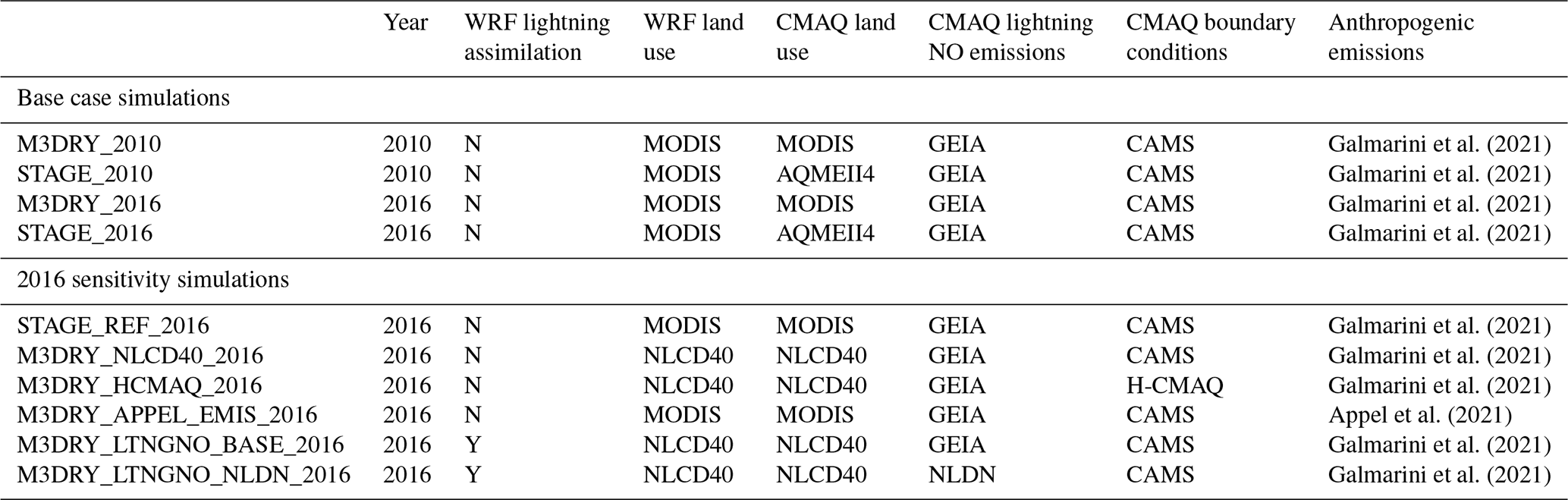
Besides the 2010 and 2016 CMAQ M3Dry and STAGE base case simulations described in Sect. 2.1, additional CMAQ sensitivity simulations were performed for 2016 to quantify the impacts of some of the differences relative to the Appel et al. (2021) CMAQ configuration and to gain further diagnostic understanding on the choice of model inputs on modeled deposition. Table 1 provides a listing of all base case and sensitivity simulations, their acronyms used in the following analyses and discussions, and the input datasets and/or configuration options differentiating them. As discussed further in Sect. 2.3, STAGE_REF_2016 is designed to quantify the impact of modifying the CMAQ STAGE code for AQMEII4 relative to the unmodified STAGE code in CMAQv5.3.1. M3DRY_NLCD40_2016 is designed to study the impact of using a different LU classification scheme in both WRF and CMAQ on simulated concentrations, deposition fields, and deposition diagnostics. M3DRY_HCMAQ_2016 can be used to assess the impact of using chemical boundary conditions from CAMS compared to using boundary conditions from H-CMAQ as in Appel et al. (2021), while M3DRY_APPEL_EMIS_2016 can be used to quantify the impacts of the different anthropogenic and wildland fire emissions used in this study vs. Appel et al. (2021). Finally, the set of M3DRY_LTGNO_BASE_2016 and M3DRY_LTGNO_NLDN_2016 simulations can be used to study the impacts of different lightning NO emission representations (GEIA vs. NLDN) on simulated concentration and deposition fields. It should be noted that these two simulations used the 2021 WRFv4.1.1 fields from Appel et al. (2021) rather than those used for the base case simulations described in Sect. 2.1.1. Because these sensitivity simulations were performed for 2016, the focus of the analysis in Sect. 3 will be on that year.

Table 1 Configurations of the AQMEII4 CMAQ simulations performed for this study.

2.3 Application of M3Dry and STAGE for AQMEII4

A key component of the AQMEII4 activity is to compute and analyze dry deposition pathways and component resistances on both a grid-scale and LU-specific basis (Galmarini et al., 2021). This section describes how this diagnostic information is generated from the CMAQ simulations contributed to the AQMEII4 activity and analyzed in this study. A schematic representation of both M3Dry and STAGE and equations for the computations of the AQMEII4 dry deposition diagnostic variables can be found in Appendix B of Galmarini et al. (2021). As described in Appel et al. (2021), both M3Dry and STAGE originate from earlier versions of the M3Dry scheme, which has a long history in CMAQ and other chemical transport models (Pleim et al., 1984). However, both algorithms follow different approaches in terms of their consideration of sub-grid-scale variations in LU and the calculation of some component resistances.

2.3.1 M3Dry

The M3Dry dry deposition calculations performed in CMAQ are designed to maintain maximum consistency with the flux calculations performed in the WRF PX LSM. Specifically, the M3Dry calculations are performed on a grid-scale basis. Sub-grid-scale variations in LU are accounted for by computing relevant grid-scale parameters like roughness length (z₀), vegetation fraction (VEGF), and leaf area index (LAI) as LU-weighted averages from LU-specific lookup table values. Grid-scale aerodynamic resistance (R_a), stomatal resistance (R_s), friction velocity (u_*), VEGF, and LAI computed in the WRF PX LSM are directly used in the CMAQ M3Dry calculations. To compute the LU-specific and grid-scale dry deposition diagnostic variables required for AQMEII4 (Galmarini et al., 2021), a post-processing tool was developed to estimate these variables by performing M3Dry calculations separately for each LU category encountered in a grid cell. While these LU-specific post-processor calculations used the same formulations and parameter values as the grid-scale deposition calculations performed in CMAQ M3Dry, the fact that WRF PX LSM uses parameter values weighted by LU fraction for the calculation of R_a, R_s, and other relevant variables means that the LU-weighted averages of the LU-specific post-processor estimates for deposition velocity (V_d) and effective conductance may slightly deviate from the grid-scale CMAQ M3Dry calculations and should therefore be viewed as an approximation. However, the LU-specific dry deposition fluxes computed by the post-processor were normalized by the grid cell values so that the LU-weighted flux sums equal the total grid cell fluxes. The CMAQ M3Dry calculations and post-processor estimates of LU-specific and aggregated diagnostic variables were performed using the native 20-category MODIS LU scheme (or 40-category NLCD LU scheme for the M3DRY_NLCD40_2016 sensitivity simulation) that was also used in the WRF simulations. Aggregation to the 16-category AQMEII4 LU scheme used in our analysis (Galmarini et al., 2021) was performed through mapping and LU-weighted averaging of equivalent categories (Table S1 in the Supplement).

2.3.2 STAGE

The STAGE dry deposition option was first introduced in CMAQv5.3 (Appel et al., 2021). It unifies bi-directional and unidirectional deposition schemes following the resistance model frameworks of Massad et al. (2010) and Nemitz et al. (2001). In contrast to M3Dry, STAGE computes individual resistances, V_d, and deposition fluxes for each LU category present in a grid cell and then aggregates these calculations to the grid-scale value for use by the CMAQ surface exchange module. Therefore, some of the deposition diagnostics required for AQMEII4 (LU-specific and grid-scale V_d and fluxes) were readily available from the standard version of STAGE in CMAQv5.3.1. Code modifications were made to output the desired component resistances and conductances that were computed but not output in the standard version of STAGE. Moreover, the STAGE code used in this study was also modified to perform all deposition calculations directly on the 16 AQMEII4 LU categories (Galmarini et al., 2021) rather than the 20 MODIS categories used in the WRF PX LSM calculations. This was accomplished by applying the same mapping used in the M3Dry post-processing and shown in Table S1 and also defining LU-specific lookup table values for required parameters like z₀, VEGF, and LAI for each of the 16 AQMEII4 categories in the modified STAGE code. As a result of deriving grid-scale deposition-related variables from LU-specific calculations and using a more aggregated LU classification scheme with a separate set of lookup table values, some of these grid-scale variables such as R_a, R_s, u_*, VEGF, and LAI may differ from the corresponding values used in the WRF PX LSM flux calculations, creating a potential inconsistency in the treatment of surface–air exchange processes simulated in WRF PX LSM and CMAQ STAGE. It should be noted that in the most recent version of CMAQ released in October 2022 (U.S. Environmental Protection Agency, 2022), STAGE was updated to normalize LU-specific calculations for R_a, R_s, and u_* such that their aggregated grid-scale values match the grid-scale values obtained from the LSM of the driving meteorological model.

2.4 Observational data

For the performance evaluation presented in Sect. 3.1 and the Supplement, the base case CMAQ simulations were compared against observations obtained from the U.S. Environmental Protection Agency's Air Quality System (AQS; https://www.epa.gov/aqs, last access: 13 July 2023) database, the Canadian National Air Pollution Surveillance (NAPS) program (https://donnees-data.ec.gc.ca/data/air/monitor/national-air-pollution-surveillance-naps-program/, last access: 13 July 2023), and the National Atmospheric Deposition Program's National Trend Network (NADP NTN; https://nadp.slh.wisc.edu/networks/national-trends-network/). Specifically, model evaluation was performed for hourly nitrogen oxides (NO_x) and sulfur dioxide (SO₂); daily maximum 8 h average ozone (MDA8 O₃); daily PM_2.5 sulfate (SO${}_{\mathrm{4}}^{\mathrm{2}-}$), nitrate (NO${}_{\mathrm{3}}^{-}$), organic carbon (OC), elemental carbon (EC), and total PM_2.5 mass from AQS; MDA8 O₃ and hourly NO_x, SO₂, and total PM_2.5 mass from NAPS; and weekly integrated precipitation and wet deposition of SO${}_{\mathrm{4}}^{\mathrm{2}-}$, NO${}_{\mathrm{3}}^{-}$, and ammonium (NH${}_{\mathrm{4}}^{+}$) from NADP NTN. The number of 2016 (2010) AQS monitors with available observations was 425 (374) for NO_x, 464 (446) for SO₂, 1323 (1278) for MDA8 O₃, 1926 (2006) for PM_2.5 mass, 318 (398) for PM_2.5 SO${}_{\mathrm{4}}^{\mathrm{2}-}$, 312 (393) for PM_2.5 NO${}_{\mathrm{3}}^{-}$, 297 (177) for PM_2.5 OC, and 297 (177) for PM_2.5 EC. The number of 2016 (2010) NAPS monitors with available observations was 116 (100) for NO_x, 98 (95) for SO₂, 178 (168) for MDA8 O₃, and 172 (159) for PM_2.5 mass. In addition, there were 259 NADP NTN monitors that measured precipitation and SO${}_{\mathrm{4}}^{\mathrm{2}-}$, NO${}_{\mathrm{3}}^{-}$, and NH${}_{\mathrm{4}}^{+}$ wet deposition in 2016 and 237 monitors that did so in 2010. All model values were matched in time and space against the available 2010 and 2016 observations using the Atmospheric Model Evaluation Tool (AMET; Appel et al., 2011) version 1.4.

3 Results

3.1 Model performance evaluation

Comparisons of modeled and observed MDA8 O₃, SO₂, NO_x, PM_2.5, SO${}_{\mathrm{4}}^{\mathrm{2}-}$, NO${}_{\mathrm{3}}^{-}$, OC, and EC concentrations at AQS monitors; MDA8 O₃, SO₂, NO_x, and PM_2.5 at NAPS monitors; and precipitation and wet deposition of SO${}_{\mathrm{4}}^{\mathrm{2}-}$, NO${}_{\mathrm{3}}^{-}$, and NH₄ at NADP NTN monitors are presented in Figs. 1–2 and Tables 2–5. This section summarizes the performance of the M3DRY_2016, STAGE_2016, M3DRY_2010, and STAGE_2010 base case simulations. To provide context for these results, a comparison to the model performance of 2016 CMAQv5.3.1 simulations from a recent comprehensive evaluation study (Appel et al., 2021) and the differences in model configurations driving differences in model performance can be found in the Supplement (Figs. S1–S7 and Tables S2–S3). Even though the diagnostic analyses presented in subsequent sections of this paper are focused on 2016, this section documents model performance results for both 2010 and 2016 because results from the 2010 simulations will be included in forthcoming AQMEII4 analyses.

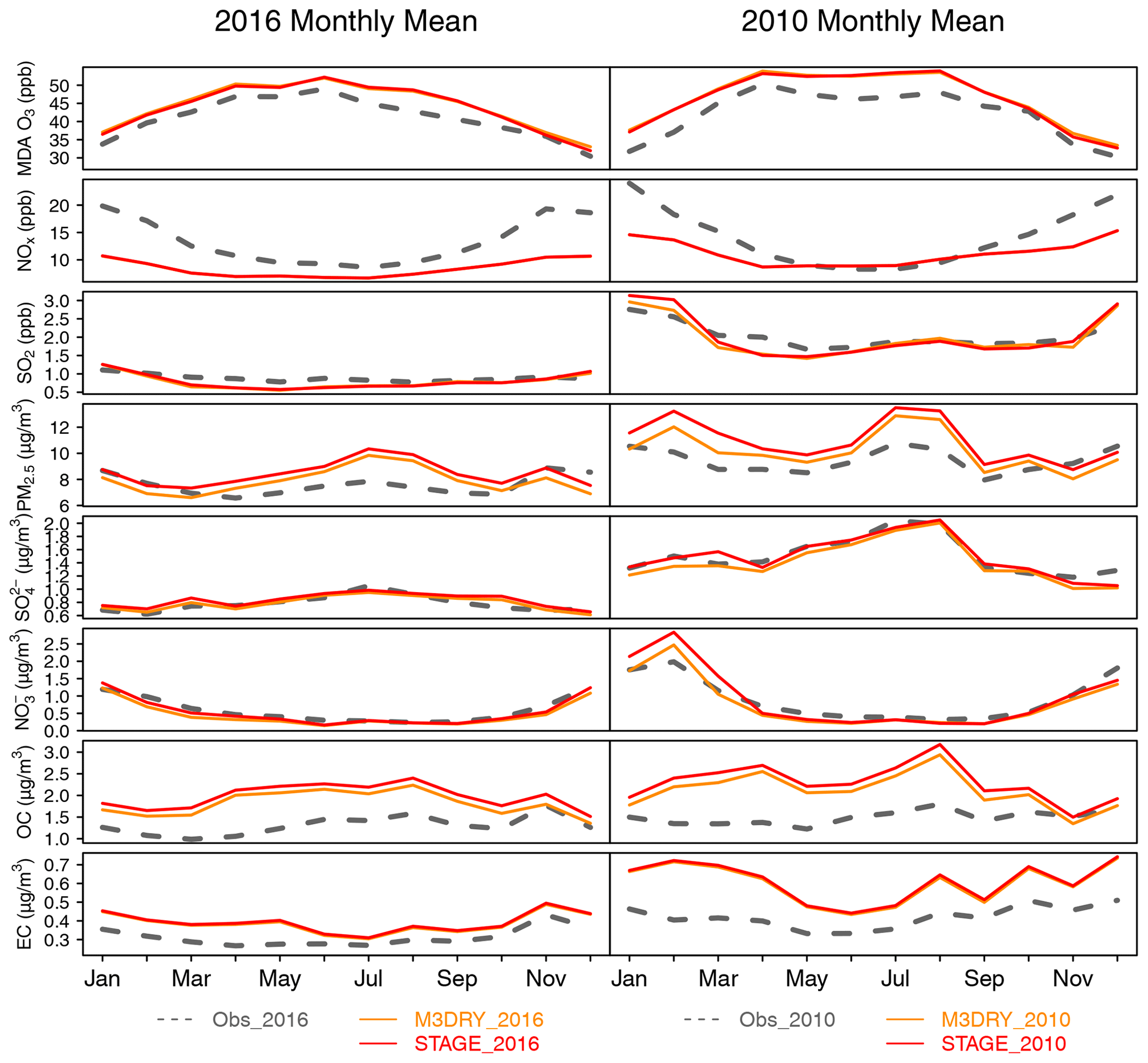
Figure 1 Monthly mean observed and modeled concentrations at AQS sites for MDA8 O₃, SO₂, NO_x, and total and speciated PM_2.5.

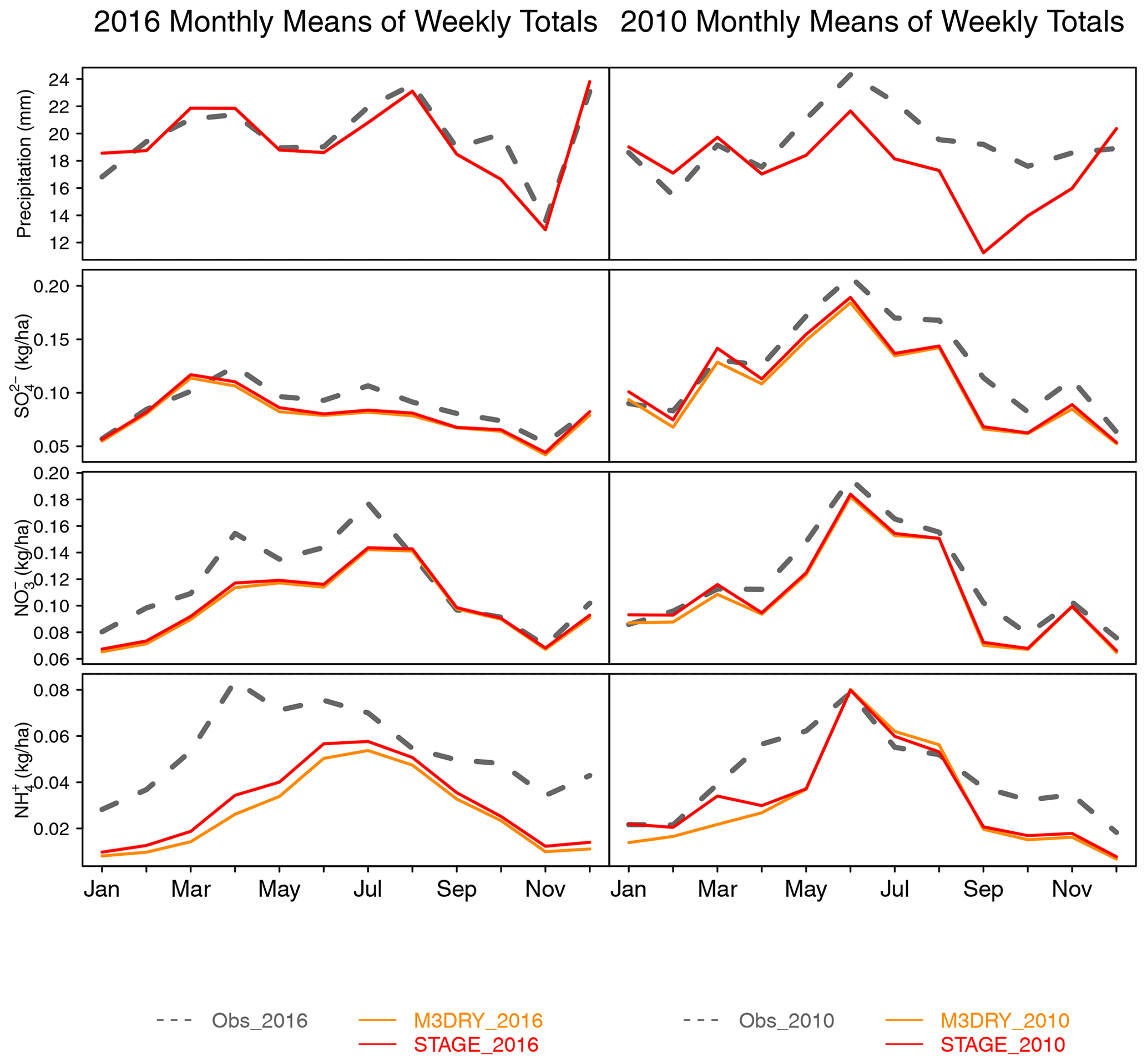
Figure 2 Monthly mean observed and modeled precipitation and wet deposition at NADP NTN sites.

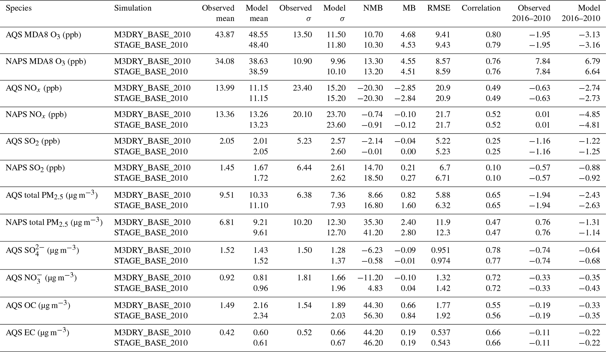
Table 2 shows key model performance metrics for the M3DRY_2016 and STAGE_2016 base case simulations for the gas phase and aerosol species listed above. These performance metrics are the observed and modeled mean values and standard deviations, the normalized and absolute mean bias (NMB and MB, respectively), the root-mean-square error (RMSE), and the correlation coefficient. The metrics shown in this table were computed across all stations and available observation–model pairs for the entire year. Corresponding time series of monthly mean observed and modeled values are shown in the left column of Fig. 1.

Table 2 Model performance statistics for all daily maximum 8 h average O₃ (MDA8 O₃), hourly NO_x and SO₂, and 24 h average total and speciated (SO${}_{\mathrm{4}}^{\mathrm{2}-}$, NO${}_{\mathrm{3}}^{-}$, organic carbon (OC) and elemental carbon (EC)) PM_2.5 mass samples collected at AQS and NAPS monitors in 2016. The standard deviation over all samples is denoted as σ, while NMB, MB, and RMSE represent the percentage normalized mean bias, mean bias, and root-mean-square error computed over all samples, respectively.

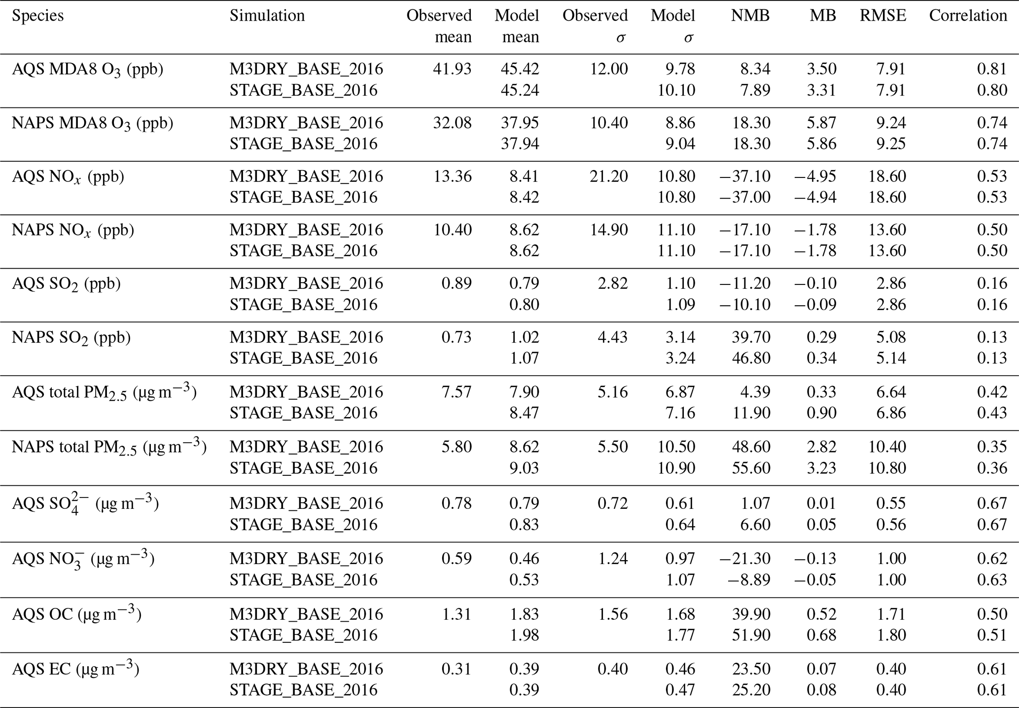
For MDA8 O₃, both simulations show positive biases of about 3.5 ppb (AQS sites) and 6 ppb (NAPS sites), RMSE values of about 8 ppb (AQS sites) and 9 ppb (NAPS sites), and correlation coefficients of about 0.8 (AQS sites) and 0.74 (NAPS sites). The differences between performance statistics for the M3Dry and STAGE simulations are small but that is partially due to the seasonally and spatially varying nature of differences between these schemes that will be discussed in Sect. 3.2. For NO_x, the simulations show substantial underpredictions that are more pronounced at the AQS than NAPS sites and correlation coefficients of about 0.5. The time series indicate that the simulations deviate most substantially from observations during winter, and differences between M3Dry and STAGE are again much smaller than differences between model values and observations. For SO₂, both the M3Dry and STAGE simulations show negative biases at AQS sites and positive biases at NAPS sites, pointing to potential differences in monitor locations relative to sources between the two networks. Correlations for SO₂ are the lowest for any of the species considered in this analysis. For PM_2.5 mass, the simulations show a positive bias that is more pronounced at NAPS than AQS monitors and correlation coefficients of about 0.4. M3DRY_2016 shows slightly lower concentrations, MBs, and RMSEs than STAGE_2016 for both networks. For PM_2.5 species, the simulations are biased high for all species except NO${}_{\mathrm{3}}^{-}$, with the highest normalized mean bias for OC. A comparison of the spatial patterns of MDA8 O₃ and PM_2.5 biases in Fig. S3 shows that the positive bias for MDA8 O₃ is widespread throughout the modeling domain, while the positive bias for PM_2.5 is most pronounced in the eastern portion of the modeling domain and some portions of the US West Coast, with smaller overestimations and some underestimations in other regions.

Table 3 and the right column of Fig. 1 show the corresponding results for the 2010 AQMEII4 simulations M3DRY_2010 and STAGE_2010. The results show that the sign of the NMB and MB for 2010 is the same as that for the 2016 results for MDA8 O₃, NO_x, SO₂, PM_2.5 mass, OC, and EC. Bias results for SO${}_{\mathrm{4}}^{\mathrm{2}-}$ and NO${}_{\mathrm{3}}^{-}$ show greater differences between the years, suggesting that the effects of the substantial reductions in SO₂ and NO_x emissions (Foley et al., 2023) between 2010 and 2016 on these aerosol species may not be captured perfectly. The observed decrease in concentrations between 2010 and 2016 is captured by both simulations for all pollutants and is likely caused in large part by substantial decreases in emissions (Foley et al., 2023), although differences in meteorological conditions between these years may also have played a role. The magnitude of the decrease is overestimated for O₃, NO_x, and PM_2.5 mass, although it is important to note that the monitors at which the statistics are calculated differ both between pollutants and between years. The differences in model performance between M3DRY_2010 and STAGE_2010 are similar to those between M3DRY_2016 and STAGE_ 2016. Tables 4–5 and Fig. 2 show model performance results for weekly precipitation and wet deposition at NADP NTN monitors in 2016 and 2010. Consistent with the negative precipitation bias, simulated wet deposition flux biases are also negative for all pollutants. This confirms that model performance for precipitation is a key driver for wet deposition model performance. The NMB results presented here fall within the range of retrospective long-term simulations over North America (Zhang et al., 2019). The results for 2010 are similar to those for 2016, again with negative biases for all variables. A comparison between 2010 and 2016 shows that the model captured the sign of the observed changes for precipitation and wet deposition fluxes, with wetter conditions in 2016 but mostly similar or slightly lower wet deposition fluxes, likely due to significant reductions in NO_x and SO₂ emissions.

Table 3 Model performance statistics for all daily maximum 8 h average O₃ (MDA8 O₃), hourly NO_x and SO₂, and 24 h average total and speciated (SO${}_{\mathrm{4}}^{\mathrm{2}-}$, NO${}_{\mathrm{3}}^{-}$, organic carbon (OC) and elemental carbon (EC)) PM_2.5 mass samples collected at AQS and NAPS monitors in 2010. The standard deviation over all samples is denoted as σ, while NMB, MB, and RMSE represent the percentage normalized mean bias, mean bias, and root-mean-square error computed over all samples, respectively. The last two columns show differences in average observed and modeled values between 2016 and 2010.

The results presented in this section demonstrate that the AQMEII4 CMAQ simulations perform similarly to other comparable regional-scale modeling studies (Emery et al., 2017; Kelly et al., 2019; Simon et al., 2012; Appel et al., 2021). The results presented in the Supplement show that the choice of the CMAQ dry deposition scheme (M3Dry vs. STAGE) has a smaller impact on aggregated model performance metrics than the sensitivity of CMAQ results to model input datasets and boundary conditions that represent the large-scale chemical environment. However, it is important to note that M3Dry and STAGE share many structural similarities (see Figs. B2 and B3 in Galmarini et al., 2021) and that the similarity in model evaluation results therefore does not imply that uncertainty in process-level representation of dry deposition is not a potentially important factor causing differences between model output and observations. An analysis of point model simulations at eight ozone flux measurement sites performed with all dry deposition schemes participating in AQMEII4 shows that differences in seasonal cycles of V_d and deposition pathways between M3Dry and STAGE are generally smaller than differences relative to other schemes. In addition, the following sections demonstrate that the choice of M3Dry vs. STAGE in CMAQ can have more pronounced impacts for specific seasons, regions, and deposition pathways than its impact on these domain-wide model performance results.

3.2 Diagnostic gas-phase dry deposition comparison M3Dry vs. STAGE

The following sections use the diagnostic variables generated for AQMEII4 to gain insights into the processes causing differences between the M3Dry and STAGE CMAQ simulations. This analysis starts with a comparison of grid-scale quantities, then proceeds to comparisons performed for the specific LU types defined for AQMEII4 (Galmarini et al., 2021), and finally compares and discusses different approaches for handling sub-grid LU variations and LU aggregation in M3Dry and STAGE. To avoid repetition, all analyses in these sections focus on the CMAQ AQMEII4 simulations performed for 2016 because the differences between the M3Dry and STAGE CMAQ simulations for 2010 were very similar to those for 2016 and because the sensitivity simulation quantifying the impacts of using a different LU classification scheme was performed for 2016.

3.2.1 Grid-scale dry deposition diagnostics and fluxes

Figure 3 shows differences in seasonal mean O₃ V_d and mixing ratios between M3DRY_2016 and STAGE_2016. It can be seen that the spatial patterns of differences in V_d and O₃ mixing ratios are closely linked, with areas of positive (negative) V_d differences between M3Dry and STAGE generally corresponding to areas of negative (positive) mixing ratio differences. During summer, M3Dry has higher V_d and lower mixing ratios than STAGE for much of the eastern US, while the reverse is the case over eastern Canada and along the US West Coast. In contrast, during winter STAGE has higher V_d and lower mixing ratios than M3Dry over most of the southern half of the modeling domain, while the reverse is the case for much of the northern US and southern Canada. The differences in seasonal mean mixing ratios reach 2–3 ppb in a number of locations, indicating that the effects of different dry deposition schemes can be more pronounced locally than in the spatially aggregated metrics presented in Sect. 3.1.

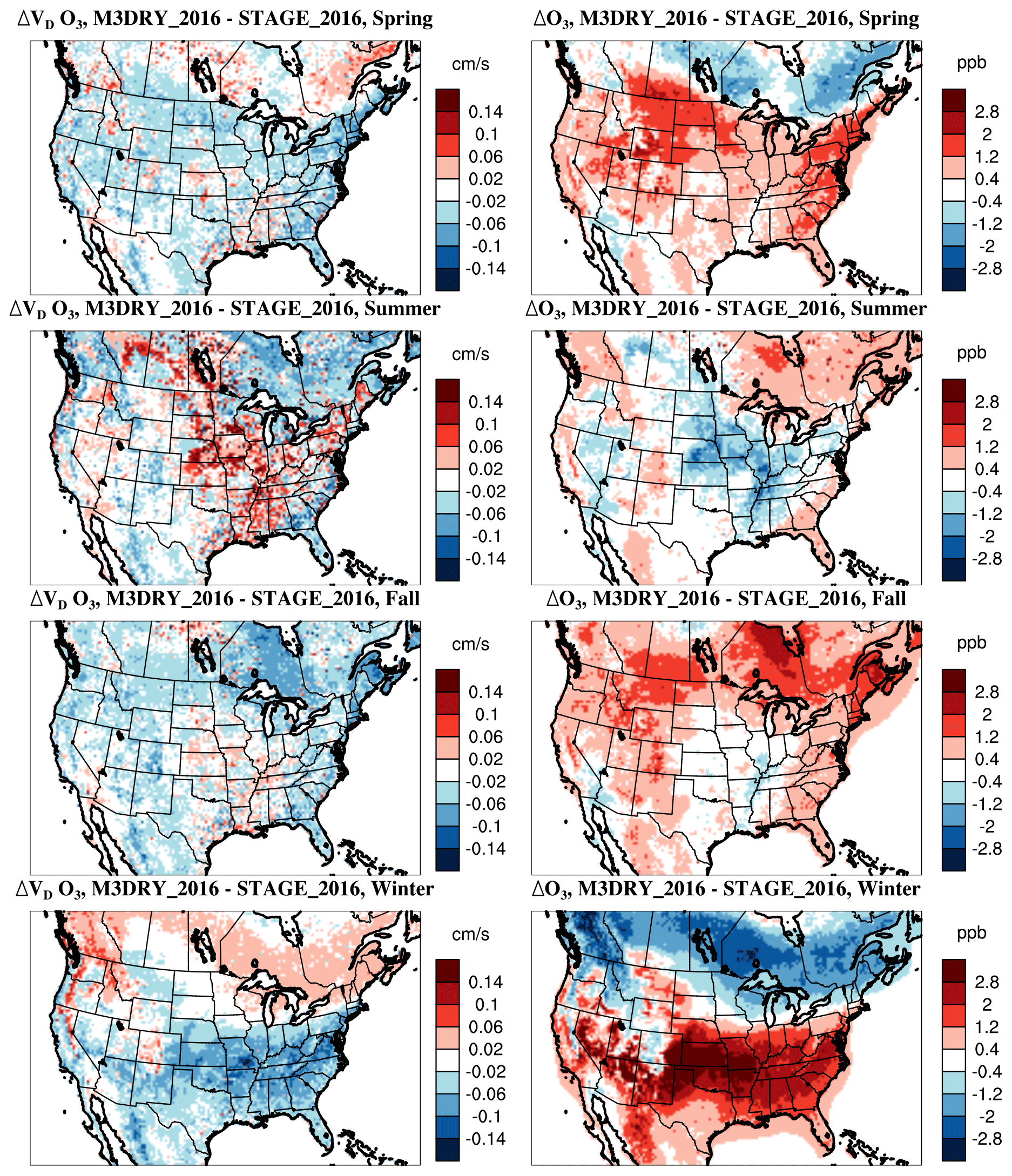
Figure 3 Differences in seasonal mean O₃ deposition velocities and mixing ratios M3DRY_2016 minus STAGE_2016.

To diagnose reasons for the differences in V_d between M3Dry and STAGE, we apply the concept of effective conductances (Paulot et al., 2018; Clifton et al., 2020b) as adapted for AQMEII4 (Galmarini et al., 2021). Given that the sum of the effective conductances equals V_d, this allows an attribution of V_d to distinct pathways controlled by different processes. The four pathways defined in Galmarini et al. (2021) and based on the original Wesely (1989) scheme are stomatal, cuticular, lower canopy, and soil. Neither M3Dry nor STAGE include a deposition pathway to the lower canopy (see Figs. B2 and B3 in Galmarini et al., 2021), but both of them distinguish between deposition to bare vs. vegetated soil, with the latter including an additional in-canopy convective resistance term. Therefore, we analyzed effective conductances for the stomatal, cuticular, vegetated soil, and bare soil pathways. We also note that the effective conductances analyzed here represent grid-scale values calculated from LU-weighted averages of the corresponding LU-specific diagnostic variables requested for AQMEII4.

Seasonal average effective conductance maps for each pathway for M3Dry and STAGE, as well as their differences, are shown in Fig. 4 for summer and in Fig. 5 for winter. Average diurnal cycles for summer and winter computed over all non-water grid cells are shown in Fig. 6 (absolute effective conductances) and Fig. 7 (percentage contribution to V_d). Figures 4–5 show that the absolute and relative magnitude of the different pathways varies both spatially and seasonally for both M3Dry and STAGE, with a generally greater importance being placed on the stomatal and cuticular pathways in the more vegetated eastern and northern portions of the modeling domain, especially during summer, and a greater importance being placed on the deposition to soil, especially bare soil, in the southwestern portion of the modeling domain and during winter. The comparison between M3Dry and STAGE shows generally higher summertime stomatal and wintertime cuticular effective conductances for M3Dry and generally higher soil effective conductances (both vegetated and bare) for STAGE in both summer and winter. The diurnal cycles in Figs. 6–7 confirm the seasonal variations and differences between M3Dry and STAGE shown in Figs. 4–5 and also illustrate the strong diurnal variation in several pathways, especially the stomatal pathway. In a relative sense, the stomatal effective conductance accounts for about half of the total V_d during daytime hours in summer, though these diurnal cycles represent an average over the entire domain, meaning that the contribution would be expected to be higher over the eastern portion of the modeling domain and lower over the southwestern portion of the modeling domain.

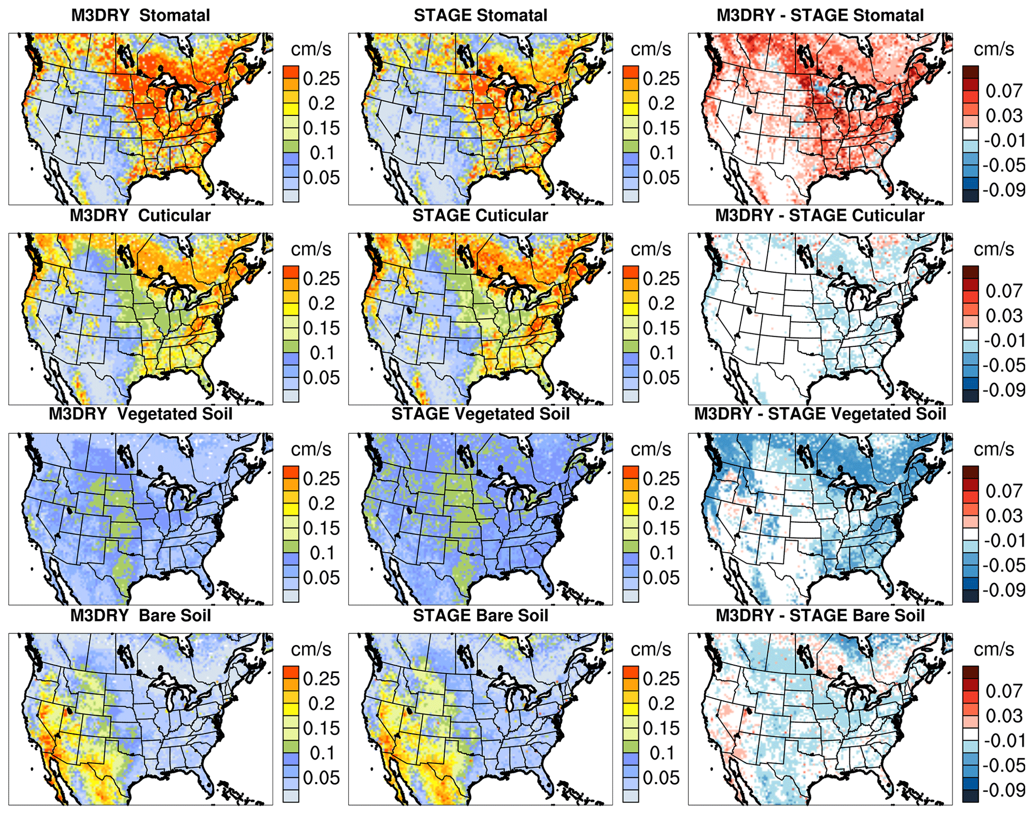
Figure 4 Grid-scale O₃ summer mean effective conductance maps for the stomatal, cuticular, vegetated soil, and bare soil pathways for M3DRY_2016, STAGE_2016, and M3DRY_2016 minus STAGE_2016.

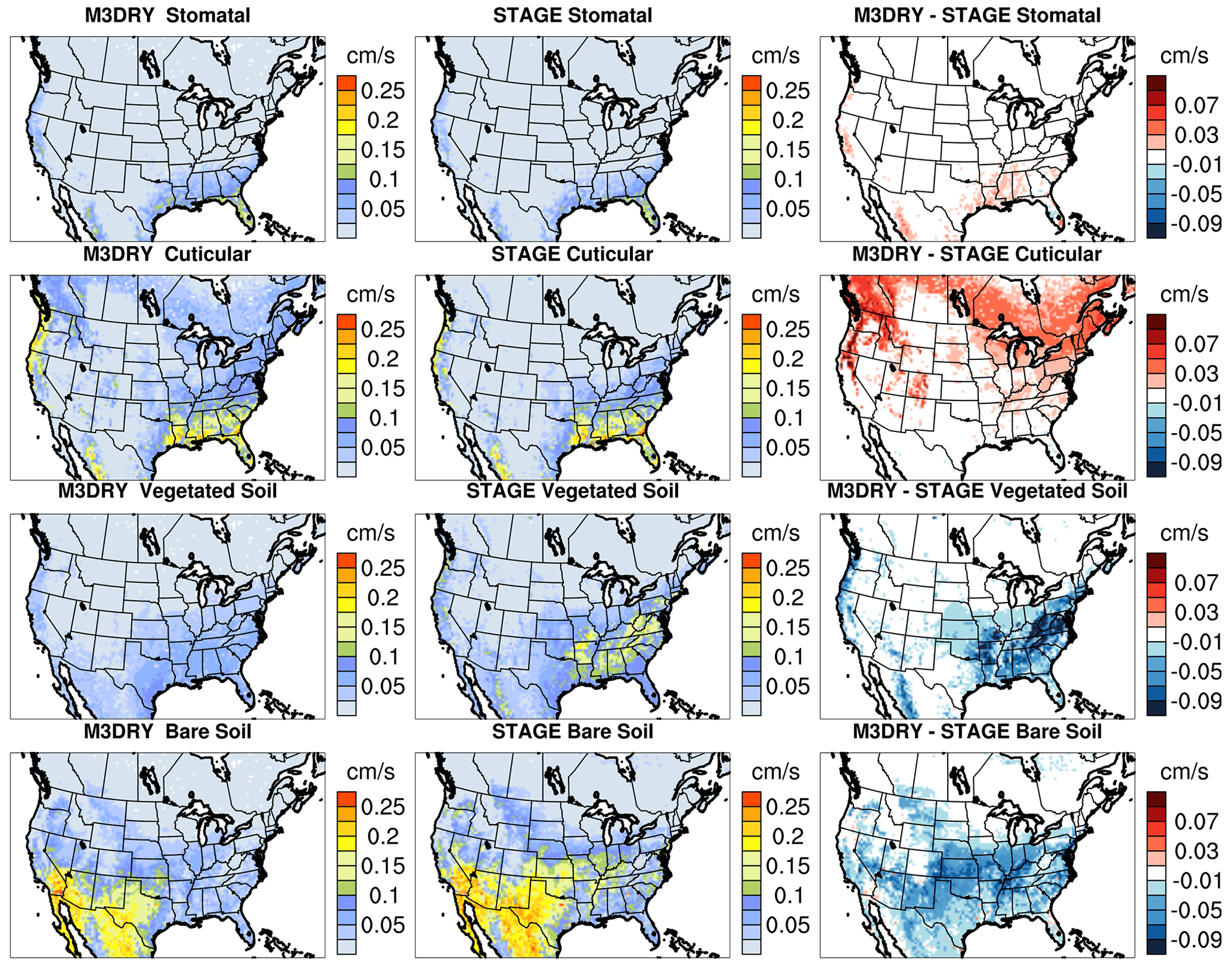
Figure 5 The same as in Fig. 4 but for winter mean effective conductances.

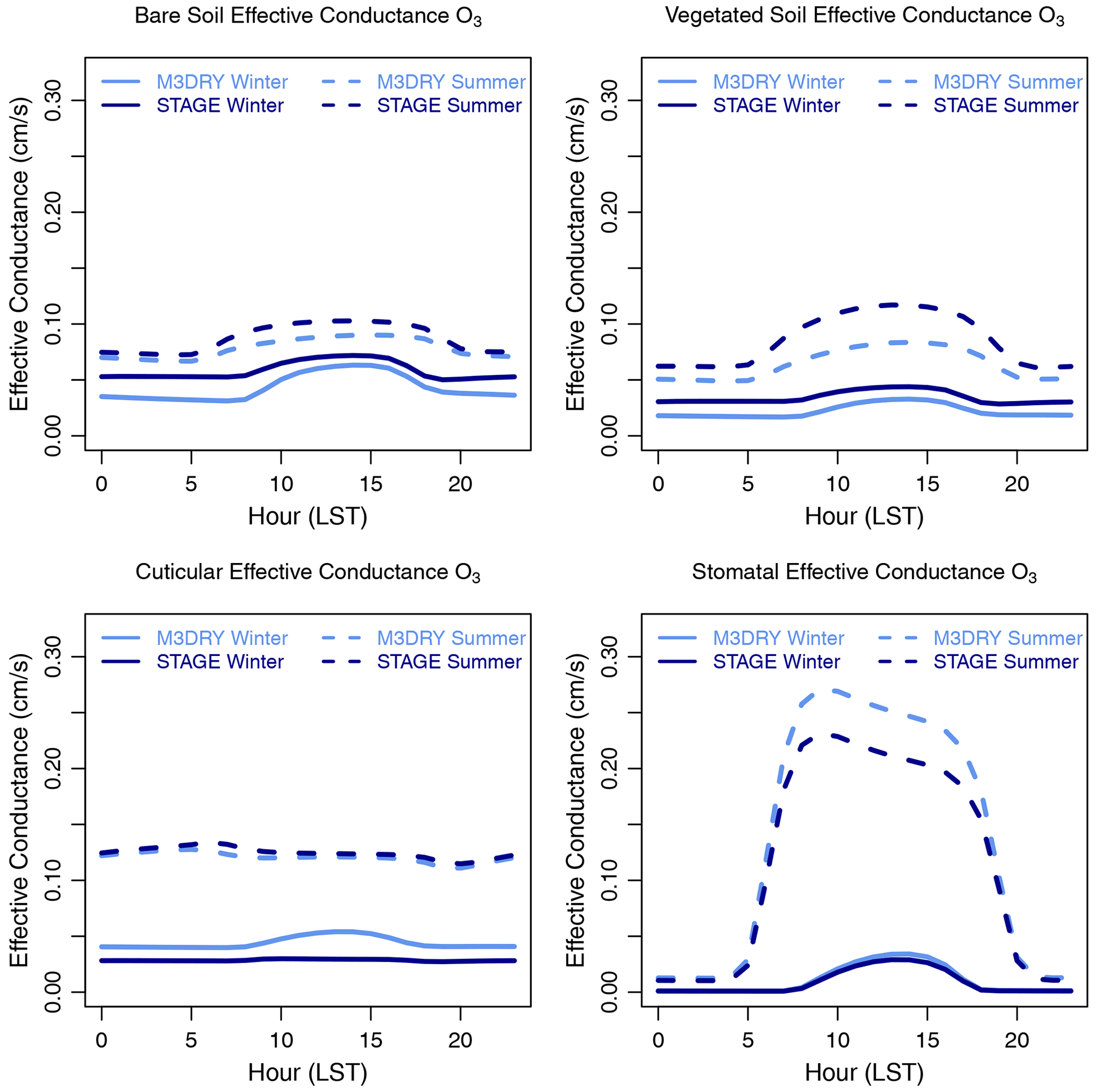
Figure 6 Summer and winter domain-average diurnal cycles of grid-scale O₃ effective conductances for the stomatal, cuticular, vegetated soil, and bare soil pathways for M3DRY_2016 and STAGE_2016.

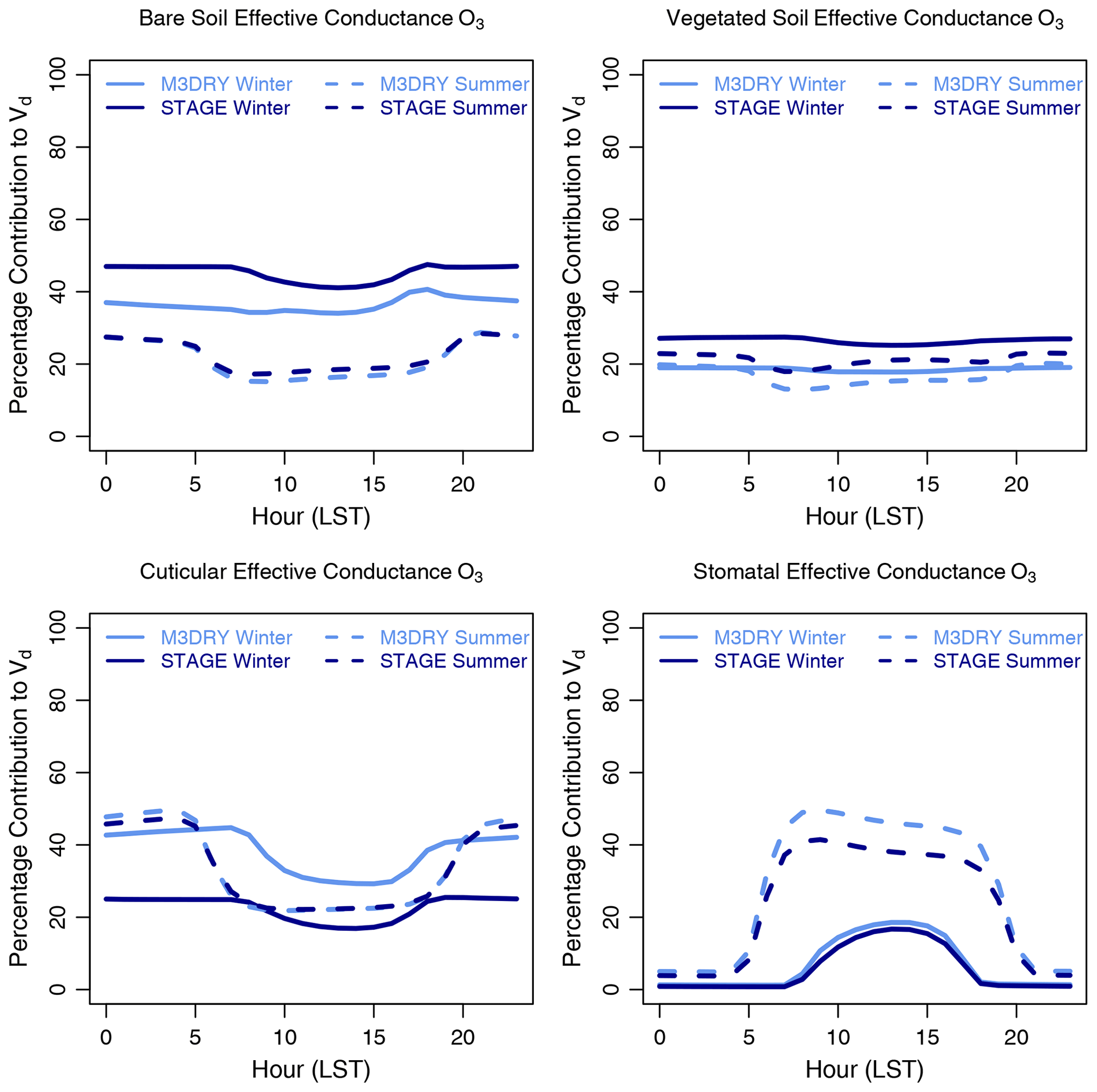
Figure 7 The same as in Fig. 6 but showing the percentage contribution of the effective conductance for each pathway to the total deposition velocity.

Comparing the effective conductance difference maps in the right columns of Figs. 4–5 to the summer and winter V_d difference maps in Fig. 3 shows that the higher summer M3Dry V_d values over the eastern US are largely due to a larger stomatal conductance. While the M3Dry stomatal conductance is also moderately larger than for STAGE over eastern Canada, this is counteracted by a substantially larger STAGE soil effective conductance, leading to a net negative difference between M3Dry and STAGE V_d values over that region. Similarly, the split between larger winter STAGE V_d over the southern portion of the domain and larger M3Dry V_d over much of the Canadian portion of the modeling domain is the result of substantially larger STAGE soil effective conductances, with only small differences in stomatal and cuticular effective conductances over the southern portion of the domain, and substantially larger cuticular effective conductances in M3Dry, with only small differences in soil effective conductances over the Canadian portion of the modeling domain.

In addition to the effective conductances, AQMEII4 also requests participating models to save and submit key component resistances common to all schemes (see Galmarini et al., 2021, Table 4 for a listing of all requested component resistances and Tables B2 and B3 for their definition in the M3Dry and STAGE deposition diagrams in Figs. B2 and B3). Like for the effective conductances, these diagnostic variables are calculated for each LU category, and grid-scale values are calculated as LU-weighted averages from LU-specific values. Figure 8 shows average summer and winter diurnal cycles of six inverse component resistances averaged over all non-water grid cells for both M3Dry and STAGE. These component resistances are the stomatal (R_s), cuticular (R_cut), in-canopy convective (R_dc), quasi-laminar sublayer (R_b for M3Dry and R_can,qlsb and R_gnd,qlsb for STAGE), and aerodynamic (R_a) resistances, and they are plotted as inverse resistances for easier comparison to V_d and effective conductances. As seen in Galmarini et al. (2021) Figs. B2 and B3, R_s, R_cut, and R_dc are pathway specific and parallel to each other, while they are also serial with R_a and the quasi-laminar sublayer resistance. In M3Dry, the quasi-laminar sublayer resistance is pathway independent, while in STAGE it differs between the canopy (cuticular and stomatal) and ground (vegetated and bare soil) pathways. Note that the y-axis range differs across different resistances to better highlight seasonal variations and differences between M3Dry and STAGE for a given resistance.

Table 4 Model performance statistics for all weekly total precipitation and SO${}_{\mathrm{4}}^{\mathrm{2}-}$, NO${}_{\mathrm{3}}^{-}$, and NH${}_{\mathrm{4}}^{+}$ wet= deposition samples collected at NADP monitors in 2016. The standard deviation over all samples is denoted as σ, while NMB, MB, and RMSE represent the percentage normalized mean bias, mean bias, and root-mean-square error computed over all samples, respectively.

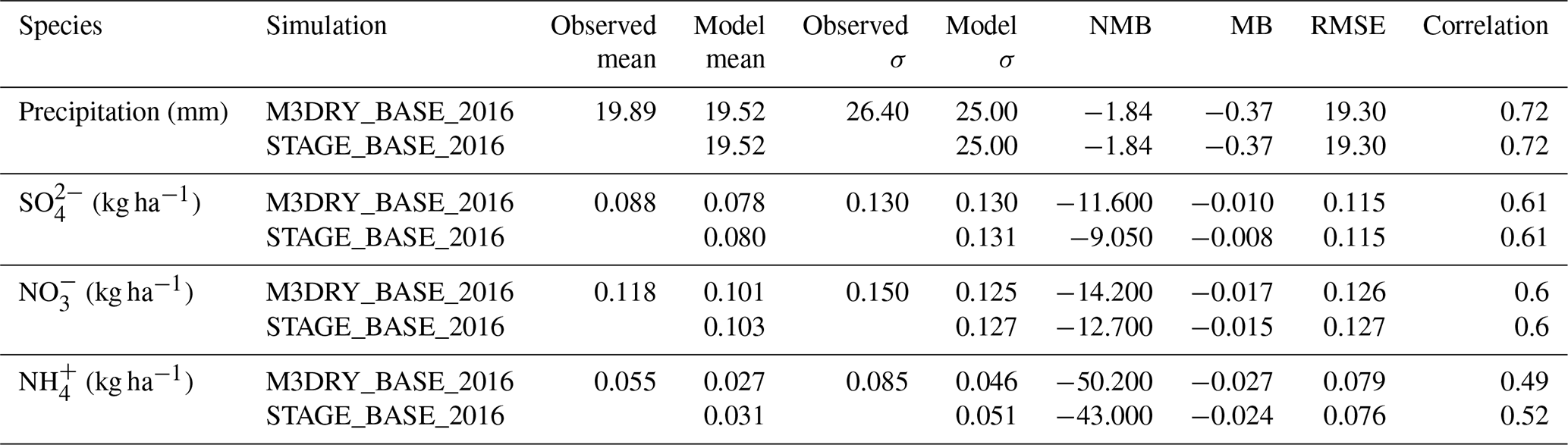
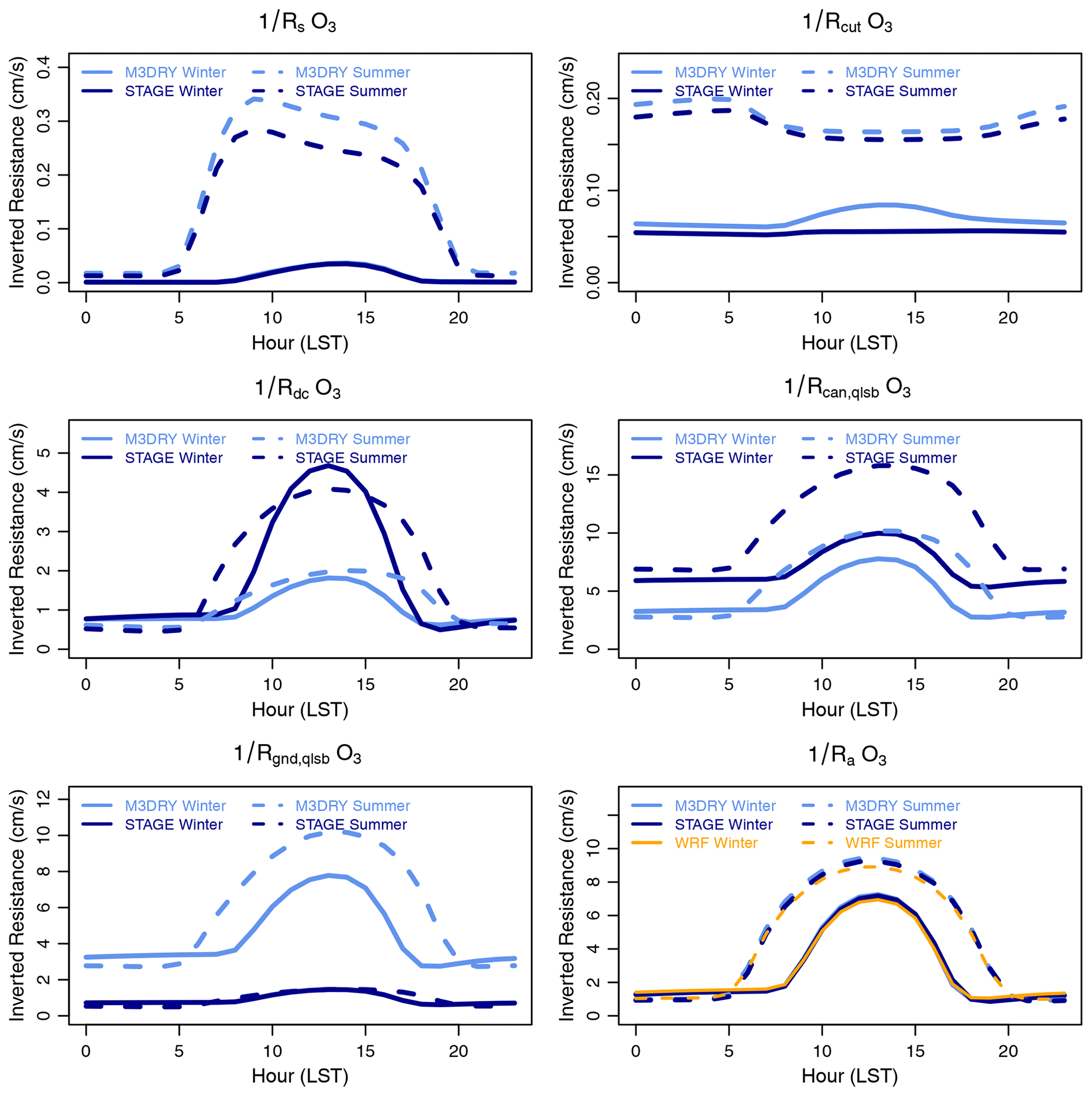
Figure 8 Summer and winter domain-average diurnal cycles of grid-scale O₃ component resistances for M3DRY_2016 and STAGE_2016. Note the different y-axis ranges for different inverted resistances. The panel showing results for the inverted aerodynamic resistance $\mathrm{1}/R_{\mathrm{a}}$ also includes the values computed in the WRF PX LSM.

Consistent with the effective conductances shown above, values for summertime $\mathrm{1}/R_{\mathrm{s}}$ and wintertime $\mathrm{1}/R_{\mathrm{cut}}$ differ between M3Dry and STAGE, with the higher values of these inverted resistances in M3Dry causing higher effective conductances for these pathways. Inverted R_dc is substantially higher in STAGE than M3Dry. While soil resistance was not requested and saved as a separate term in AQMEII4 as its definition differs across schemes, the higher inverted STAGE R_dc values likely had an effect on the higher STAGE effective conductance values for the vegetated soil pathway. For the quasi-laminar sublayer resistances, inverted R_can,qlsb for STAGE is higher than the pathway-independent inverted R_b for M3Dry, which in turn is higher than the inverted R_gnd,qlsb for STAGE. However, these resistances are typically small compared to the other resistances (i.e., their inverted values are larger), meaning that they generally only have a small impact on effective conductances and overall V_d. The inverted aerodynamic resistance R_a is very similar between M3Dry and STAGE for both summer and winter. As discussed in Sect. 2.3.1, all LU-specific diagnostic deposition variables for M3Dry are estimated through a post-processor, whereas the M3Dry calculations within CMAQ used grid-scale R_a calculated by the WRF PX LSM to maintain maximum consistency between the representation of land–surface exchange processes in WRF and CMAQ. Therefore, the lower-right panel for inverted R_a also shows the WRF-based grid-scale value used in the M3Dry CMAQ deposition calculations. This value is very similar to the post-processor-based estimate for M3Dry. The different approaches taken by M3Dry and STAGE to handle sub-grid variability in LU and their impacts on deposition calculations are discussed further in Sect. 3.2.3.

While this section so far has focused on applying the AQMEII4 diagnostics to analyze M3Dry vs. STAGE differences in O₃ deposition, these diagnostics are also being calculated for SO₂, NO₂, NO, HNO₃, NH₃, PAN, HNO₄, N₂O₅, organic nitrates, H₂O₂, and HCHO (Galmarini et al., 2021). Moreover, the effective conductances and total V_d can also be used to calculate effective fluxes, i.e., apportion total dry deposition fluxes to specific pathways (Galmarini et al., 2021). Figure 9 shows annual domain-average (excluding water cells) V_d for M3Dry and STAGE for O₃, H₂O₂, HCHO, SO₂, and oxidized nitrogen species as sum of the effective conductances for the four pathways, while Fig. 10 shows the corresponding annual total domain-wide (excluding water cells) dry deposition fluxes as a sum of the effective fluxes. The V_d and deposition flux results for O₃ reflect the larger contributions from the vegetated and bare soil pathways for STAGE and the larger contributions for the stomatal and cuticular pathways for M3Dry. Annual domain total O₃ deposition fluxes differ only slightly between M3Dry and STAGE due to the seasonal and spatial variation in the V_d differences shown in Fig. 3. In contrast to O₃, most other pollutants show larger effective conductances and effective fluxes for the bare soil and the sum of bare and vegetated soil pathways for M3Dry than STAGE. The cuticular effective flux is larger for M3Dry than STAGE for HCHO, SO₂, HNO₄, and organic nitrates; smaller for M3Dry than STAGE for H₂O₂ and HNO₃; and similar between M3Dry and STAGE for other species. Stomatal effective fluxes are small for all species except O₃, HCHO, and NO₂ for both M3Dry and STAGE. Total dry deposition fluxes differ the most between M3Dry and STAGE for HCHO and organic nitrate, although it again should be noted that these fluxes represent annual domain totals and that larger differences likely exist at sub-seasonal scales for different regions.

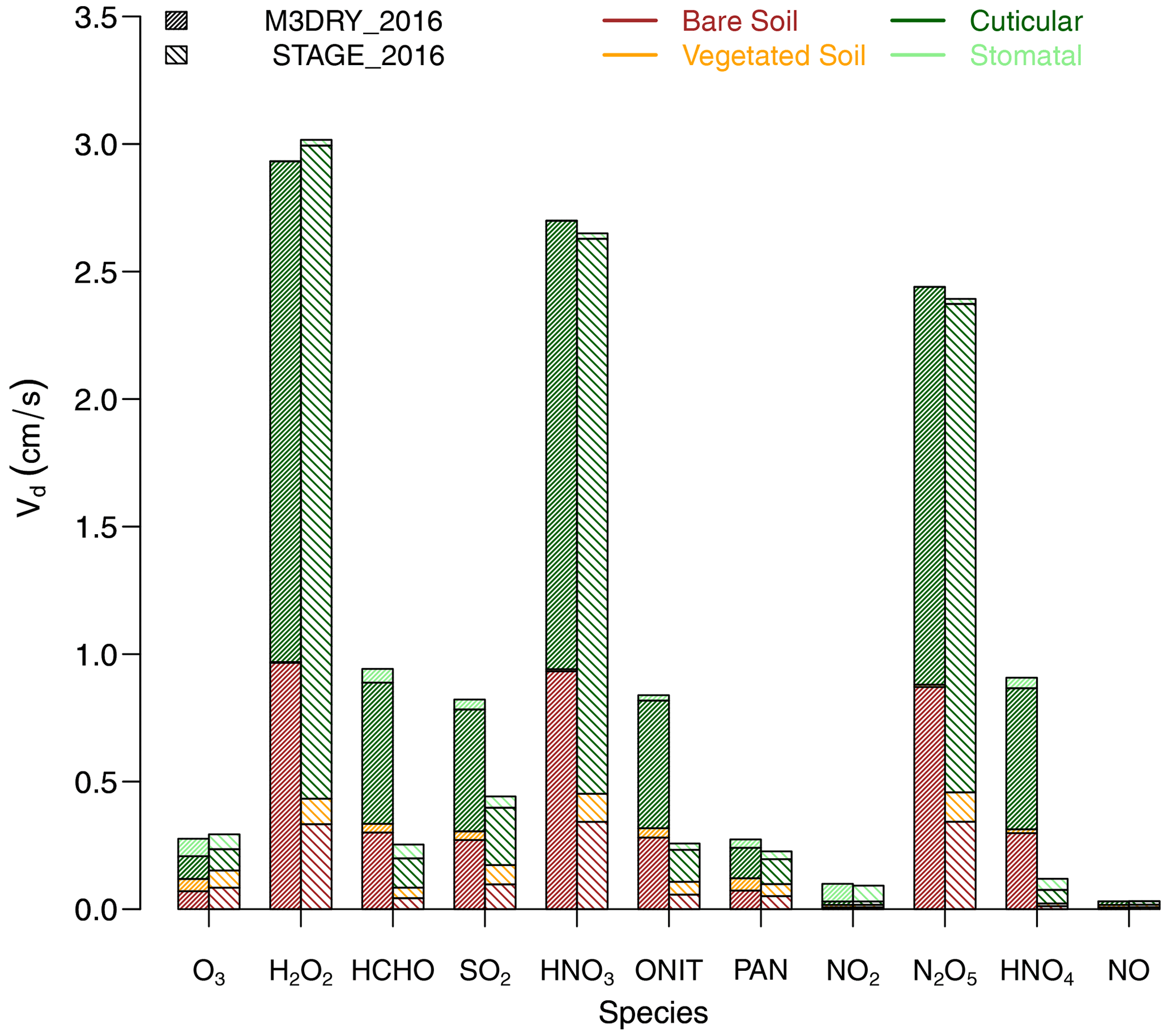
Figure 9 Grid-scale annual average domain-wide (excluding water cells) effective conductances for O₃, H₂O₂, HCHO, SO₂, and oxidized nitrogen species.

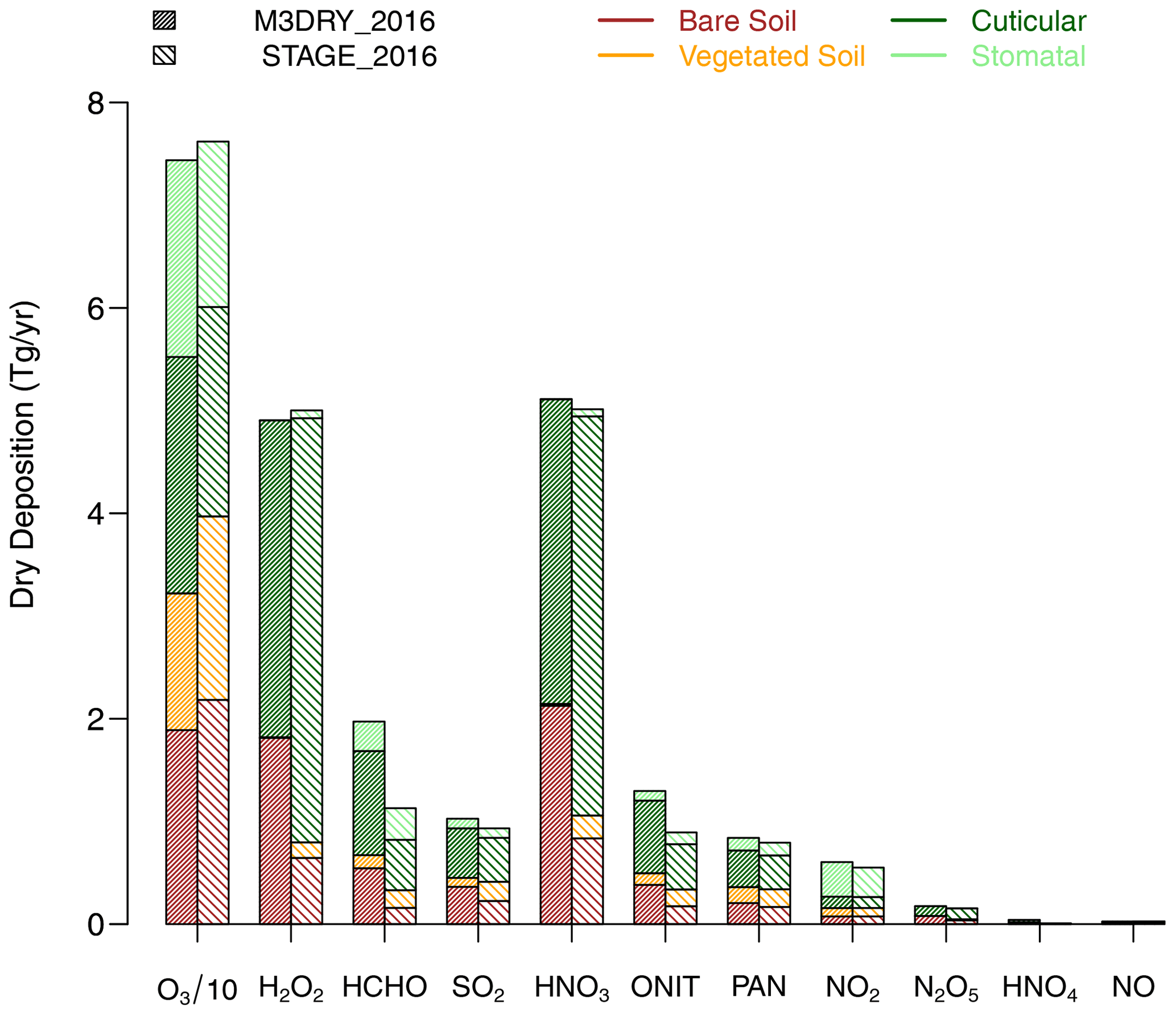
Figure 10 Grid-scale annual total domain-wide (excluding water cells) pathway-specific dry deposition fluxes (“effective fluxes”) for O₃, H₂O₂, HCHO, SO₂, and oxidized nitrogen species. Ozone dry deposition values are divided by a factor of 10 to use the same y axis as for the other pollutants.

3.2.2 LU-specific dry deposition diagnostics and fluxes

In this section, we utilize the LU-specific dry deposition diagnostics generated during AQMEII4 to provide further insights into the grid-scale comparisons presented above. These LU-specific diagnostics were generated for the 16 common LU types defined in Galmarini et al. (2021). Figure S8 depicts spatial maps of the fractional coverage for each of these 16 categories, aggregated through post-processing from the native 20 MODIS LU categories used in the M3DRY_2016 simulations (see Sect. 2.3.1). The aggregation of the MODIS LU categories to the AQMEII4 LU categories (performed during post-processing for M3Dry and prior to the deposition calculations in STAGE as discussed in Sect. 2.3.2) is documented in Table S1. Note that none of the 20 MODIS LU categories correspond to the AQMEII4 herbaceous category. Figure S8 shows the prevalence of evergreen needleleaf, mixed, and deciduous forest in the northern, northeastern, and southeastern portions of the modeling domain, planted and cultivated LU in the north-central portion of the modeling domain, grassland in a belt stretching from Texas to Montana, and shrubland in the southwestern portion of the modeling domain. Figure S9 shows bar charts of the fraction of the modeling domain covered by each LU category. Separate bar charts are shown for M3DRY_2016 and STAGE_2016. While both started with the fractional coverages of the MODIS LU categories in the 12 km modeling domain, they differ in their treatment of grid cell with partial water coverage. Consistent with the approach taken in the WRF PX LSM, M3DRY_2016 treats cells with more than 10 % water coverage as either all land or all water. For grid cells with water fractions between 10 % and 50 %, the water fraction is reset to zero, whereas the non-water categories are renormalized to 100 %. For grid cells with water fractions exceeding 50 %, the water fraction is reset to 100 %, whereas the fractions for non-water categories are set to zero. No renormalization is performed for grid cells with water fraction coverage below 10 %. The rationale for this approach is that meteorological flux calculations are distinctly different between land and water, and both WRF PX LSM and M3Dry are designed to retain the distinctiveness imposed by the underlying spatial discretization of the modeling domain. On the other hand, STAGE does not apply any special treatment to grid cells with partial water coverage. As a result of these different approaches, Fig. S9 shows that a slightly larger fraction of the modeling domain is covered by water for STAGE_2016 compared to M3DRY_2016, with correspondingly slightly smaller coverages for non-water categories.

First, we investigate summer and winter average diurnal cycles of LU-specific component resistances in the context of the grid-scale resistance shown in Fig. 8 and discussed in Sect. 3.2.1. Figure S10 shows that R_s conductances are higher for M3Dry than STAGE during summer for all forest types, agricultural land, savanna, and tundra, i.e., common LU types within the modeling domain (Figs. S8 and S9). Only wetlands have higher R_s conductance for STAGE than M3dry, with the remaining LU categories having similar R_s conductances for both schemes. This is consistent with the grid-scale domain-average summer R_s conductance being higher for M3Dry than STAGE (Fig. 8). Only small differences are seen in winter for both the grid-scale (Fig. 8) and LU-specific (Fig. S10) stomatal conductances. The higher domain-average grid-scale $\mathrm{1}/R_{\mathrm{cut}}$ conductance for M3Dry during winter (Fig. 8) is driven by the higher cuticular conductance values for evergreen needleleaf forest, mixed forest, and agricultural land (Fig. S11), particularly since these LU types cover a substantial portion of the domain (Figs. S8–S9). Figure S12 shows that the higher domain-average grid-scale in-canopy convective conductance ($\mathrm{1}/R_{\mathrm{dc}}$) for STAGE during both summer and winter (Fig. 8) is present for almost all LU categories with the exception of snow and ice, which (along with barren) uses a placeholder value to represent the non-existent canopy and is present in very few grid cells in the domain (Fig. S9). LU-specific R_can,qlsb conductances ($\mathrm{1}/R_{\mathrm{can},\mathrm{qlsb}}$) are higher for STAGE than M3Dry for almost all LU categories in both summer and winter (Fig. S13), while the opposite is the case for R_gnd,qlsb (Fig. S14). This demonstrates that the same behavior noted for the grid-scale R_can,qlsb and R_gnd,qlsb conductances (Fig. 8) was not driven by differences in their representation by M3Dry vs. STAGE for select LU categories only but rather resulted from consistent differences in representation across all LU categories. LU-specific R_a conductances ($\mathrm{1}/R_{\mathrm{a}}$) are generally very similar between STAGE and M3Dry with the exception of urban and tundra for which M3Dry is higher than STAGE and wetlands for which STAGE is higher than M3Dry (Fig. S15). This general similarity between M3Dry and STAGE is consistent with the net grid-scale domain-average R_a conductances shown in Fig. 8. Differences between grid-scale and LU-weighted aggregated LU-specific R_a are investigated further in the next section.

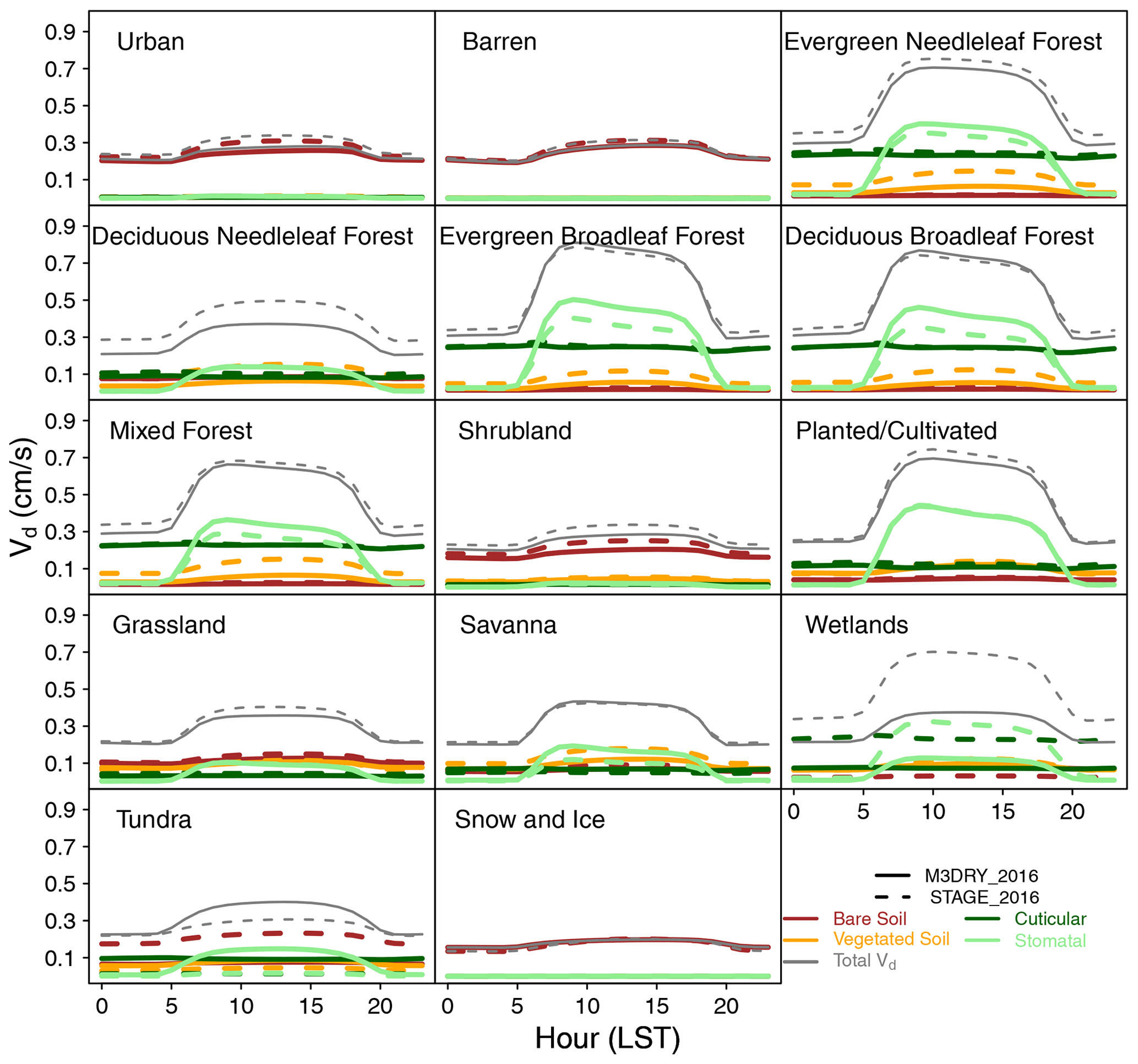
Figure 11 Summer domain-average diurnal cycles of LU-specific O₃ effective conductances and total deposition velocities for M3DRY_2016 and STAGE_2016.

Next, we investigate the effects of the differences in the LU-specific component resistances discussed above on LU-specific effective conductances and effective fluxes, i.e., pathway-specific V_d and dry deposition fluxes. Figure 11 depicts summer average diurnals of LU-specific effective conductances and total V_d for O₃ for both M3Dry and STAGE, averaged over all grid cells with a non-zero fractional coverage for a given LU category. As expected, these diurnal cycles illustrate that both total V_d and the relative importance of the different effective conductance pathways vary between LU categories for both M3Dry and STAGE as a result of different underlying surface characteristics like VEGF and vegetation type for the different LU categories. Total V_d during daytime varies by a factor of 2 between the LU categories with the lowest values (urban, barren, and snow and ice) and those with the highest values (evergreen needleleaf and broadleaf forest, deciduous forest). Effective conductances for the bare soil pathway dominate for the urban, barren, and shrubland LU categories, while conductances for the cuticular and stomatal pathways dominate for the forest LU categories, especially during daytime. Results also show that the M3Dry vs. STAGE differences are most pronounced for the stomatal and vegetated soil pathway for the forest LU categories, with M3Dry estimating larger effective conductances for the stomatal pathway and STAGE estimating larger effective conductances for the vegetated soil pathway for these LU categories. Higher effective conductances for the bare soil pathway in STAGE are particularly noticeable for the urban, shrubland, and tundra LU categories. When considering how these differences in LU-specific effective conductances impact the grid-scale summertime effective conductances shown in Figs. 4–5, the abundance and spatial distribution of each LU category (Figs. S8 and S9) needs to be taken into account. For example, given the abundance of the evergreen needleleaf forest, deciduous broadleaf forest, and mixed forest categories over the eastern and northern portions of the modeling domain, the higher M3Dry stomatal conductances and lower M3Dry vegetated soil conductances for these LU categories shown in Fig. 11 can explain the spatial pattern of the corresponding M3Dry vs. STAGE grid-scale differences for these two pathways shown in Figs. 4–5.

The analysis above provided diagnostic insights into the M3Dry vs. STAGE differences in grid-scale effective conductances shown in Figs. 4–5 and discussed in Sect. 3.2.1. Analogously, Fig. 12 shows annual and summer domain-total LU-specific effective fluxes for O₃ to provide further insights into the corresponding grid-scale effective fluxes shown in the left two bars of Fig. 10 and also discussed in Sect. 3.2.1. For annual total deposition, the overall slightly larger grid-scale O₃ deposition flux for STAGE (Fig. 10) is present for almost all LU categories, with only a few categories (e.g., evergreen needleleaf and broadleaf forest) showing no discernible differences between M3Dry and STAGE. Likewise, the generally larger contribution of the stomatal and cuticular deposition pathways in M3Dry and bare and vegetated soil in STAGE are present for most LU categories, but the differences in the magnitude of the individual deposition pathways are especially pronounced for the evergreen needleleaf forest, mixed forest, and agricultural LU categories. Considering effective fluxes for summertime only, the greater importance of the cuticular and stomatal pathways during this season for LU categories most strongly affected by seasonal variations in LAI (deciduous broadleaf forest and planted and cultivated; see Table 6), along with the greater importance of these pathways in M3Dry compared to STAGE, yield greater overall estimated deposition to these LU categories for M3Dry compared to STAGE. In contrast, for several other LU categories (e.g., evergreen needleleaf and mixed forest, shrubland, and grassland), STAGE still estimates higher deposition even during summertime, largely due to its higher estimated deposition to vegetated and bare soil and the dominance of these pathways for several of these LU categories (shrubland and grassland). Overall, Fig. 12 demonstrates that even though overall annual total O₃ deposition fluxes estimated by M3Dry and STAGE are fairly similar (Fig. 10), pathway-specific fluxes to individual LU types can vary more substantially on both annual and seasonal scales, which might affect estimates of O₃ damages to sensitive vegetation.

Table 5 Model performance statistics for all weekly total precipitation and SO${}_{\mathrm{4}}^{\mathrm{2}-}$, NO${}_{\mathrm{3}}^{-}$, and NH${}_{\mathrm{4}}^{+}$ wet deposition samples collected at NADP NTN monitors in 2010. The standard deviation over all samples is denoted as σ, while NMB, MB, and RMSE represent the percentage normalized mean bias, mean bias, and root-mean-square error computed over all samples, respectively. The last two columns show differences in average observed and modeled weekly total values between 2016 and 2010.

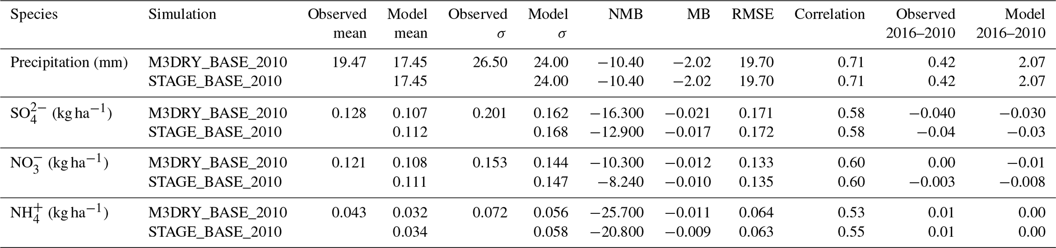
Table 6 LU-specific lookup table parameter values for seasonal minimum and maximum leaf area index (LAI), seasonal minimum and maximum vegetation fraction (VEGF), and surface roughness (z₀) used in the dry deposition calculations. See the beginning of Sect. 3.2.2 for details on the differences between the “PX LSM/M3DRY”, “STAGE”, and “STAGE REF” columns for each variable. The boldfaced entries indicate instances where parameter values differed between the WRF PX LSM (also used in M3DRY) and the STAGE AQMEII4 and/or STAGE reference configuration.

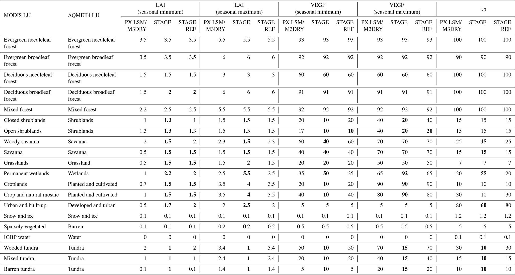
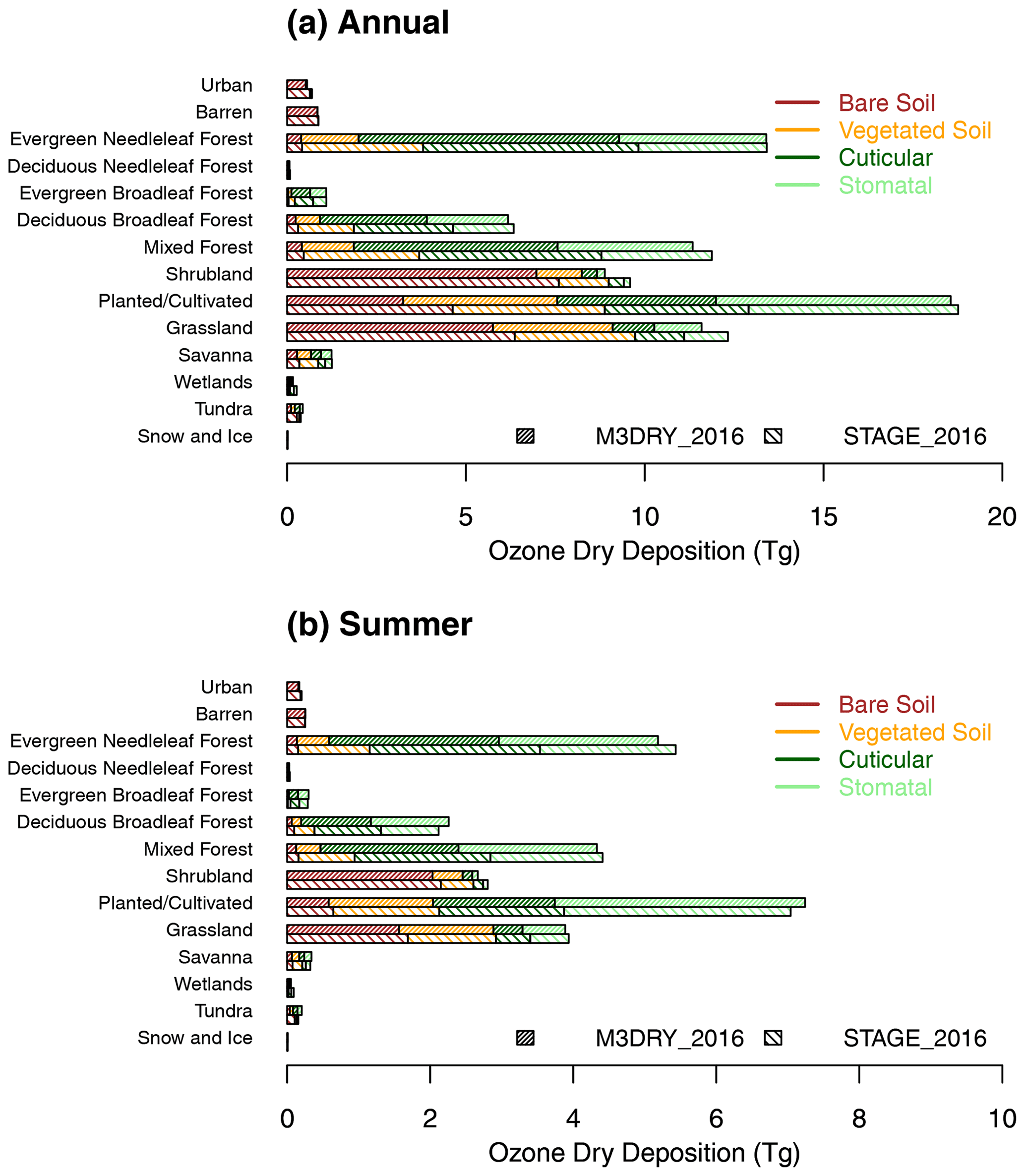
Figure 12 Land-use-specific domain-wide (excluding water cells) pathway-specific O₃ dry deposition fluxes (“effective fluxes”): (a) annual and (b) summer values.

3.2.3 Impact of different approaches for handling subgrid LU variations and LU aggregation in M3Dry and STAGE

Both WRF PX LSM (M3Dry) and STAGE rely on LU-specific parameters prescribed in lookup tables to account for subgrid-scale LU variations when performing grid-scale calculations. As discussed in Sect. 2.3.1 and 2.3.2, the WRF PX LSM bases grid-scale calculations on LU-weighted aggregated parameters from such LU-specific lookup table values and CMAQ M3Dry then directly uses these calculations in its grid-scale deposition calculations, maintaining consistency with WRF PX LSM. On the other hand, CMAQ STAGE and the M3Dry post-processor developed for AQMEII4 perform LU-specific deposition calculations using the lookup table values for each LU type, and in the case of CMAQ STAGE then use these LU-specific deposition calculations to calculate grid-scale deposition, maintaining consistency between LU-specific and grid-scale deposition but potentially differing from WRF PX LSM for variables like R_a, R_s, and u_* (note that starting with CMAQv5.4, released in October 2022, STAGE normalizes R_a, R_s, and u_* to match the aggregated grid-scale values to the grid-scale values calculated in the LSM of the driving meteorological model). To provide further context for these differences, Table 6 documents several of these LU-specific lookup table parameters used in deposition calculations, i.e., LAI, VEGF, and z₀. Values are shown for the 20 LU category MODIS configuration of WRF PX LSM and M3Dry, the 16 LU category AQMEII4 configuration of STAGE used in this study, and the 20 LU category MODIS configuration in the unmodified version of STAGE used for sensitivity simulation STAGE_REF_2016 discussed below. The boldfaced entries indicate instances where parameter values differed from WRF PX LSM (and M3Dry) for the STAGE AQMEII4 and/or STAGE MODIS configuration. For example, STAGE prescribes lower z₀ for the urban and tundra categories for both the AQMEII4 and MODIS configurations and higher z₀ for wetlands for the AQMEII4 configuration. These differences in z₀ are consistent with the $\mathrm{1}/R_{\mathrm{a}}$ differences for these three LU categories shown in Fig. S15. The higher wetlands z₀ specified in STAGE results in lower R_a and higher $\mathrm{1}/R_{\mathrm{a}}$ compared to M3Dry, while the reverse is true for the tundra and urban categories.

Figures S16 and S17 compare grid-scale vs. LU-weighted aggregates of LU-specific values for u_* and R_a for both M3Dry and STAGE. For M3Dry, the sum of the LU-weighted aggregated u_* estimates matches the grid-scale values within 10 %, with generally larger values for the aggregated estimates. For STAGE_2016 and STAGE_REF_2016, the aggregated values also typically fall within 10 % of the grid-scale values, but differences can be both positive and negative. For R_a, differences between the LU-weighted aggregated and grid-scale values can reach 25 % for all cases examined here, with generally higher values for the LU-weighted aggregated R_a values, which is consistent with Fig. 8.

Figure 13 compares seasonal mean O₃ V_d and mixing ratio differences between STAGE_2016 and STAGE_REF_2016 to assess the impact of performing STAGE deposition calculations on the more aggregated 16-category AQMEII4 LU classification scheme (see Sect. 2.3.2) rather than the 20-category MODIS LU classification scheme used in the WRF PX LSM. Results show that the use of the AQMEII4 LU classification scheme can cause seasonal mean O₃ V_d increases of 0.02–0.06 cm s⁻¹ and corresponding season mean O₃ mixing ratio decreases of 0.5–1 ppb mostly over the eastern and northern portions of the modeling domain. The location of these changes suggests that they are likely at least partially due to the collapsing of two MODIS agricultural LU categories (croplands and crop/natural mosaic) with different lookup table values to a single AQMEII4 agricultural LU category (see Table 6 and Fig. S8).

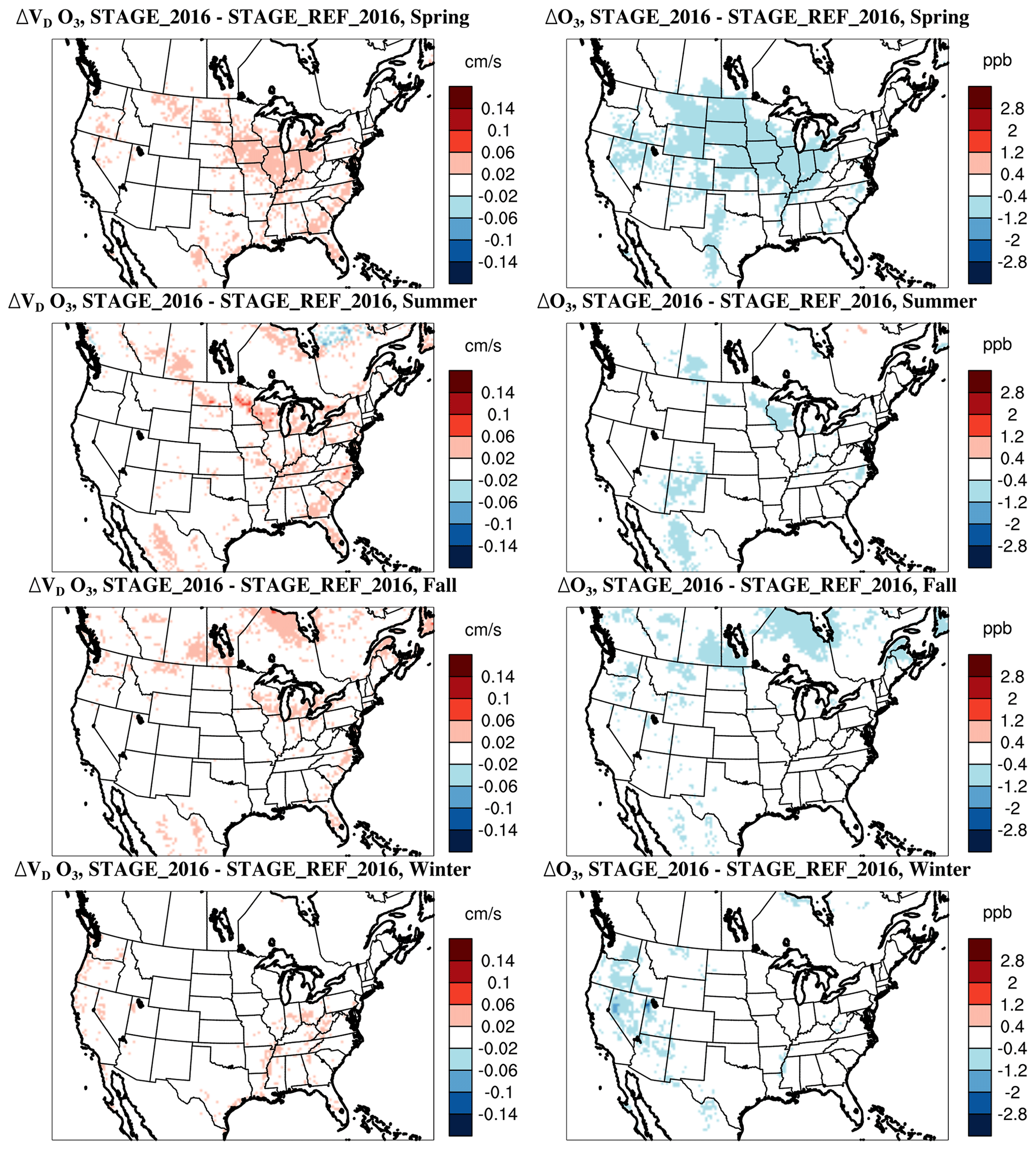
Figure 13 Differences in seasonal mean O₃ deposition velocities and mixing ratios STAGE_2016 minus STAGE_2016_REF.

The results presented in this section showed that differences in LU-specific lookup table values between different deposition schemes and/or between the WRF PX LSM calculations and the deposition scheme calculations within CMAQ, as well as the aggregation of the MODIS LU categories to the AQMEII4 LU categories in the STAGE deposition calculations, can introduce differences in the estimated V_d and resulting mixing ratios. In the next section, we investigate the effects of using a different underlying LU classification scheme in both the WRF PX LSM calculations and the CMAQ M3Dry calculations.

3.3 Impacts of land-use classification scheme

In this section, we compare the effects of replacing the MODIS dataset to represent LU in both WRFv4.1.1 and CMAQ M3Dry with the National Land Cover Dataset (NLCD) (Dewitz and U.S. Geological Survey, 2021; Yang et al., 2018). Similar comparisons between the U.S. Geological Survey (USGS) and NLCD LU datasets in WRF have previously been presented by Mallard et al. (2018). In contrast to the changes discussed in the previous section, the differences between MODIS and NLCD are due to different underlying remote sensing data, their spatial resolution, and different approaches for their classification into distinct LU categories. Specifically, the MODIS LU categorization scheme as implemented in WRFv4.1.1 uses 20 categories following the IGBP land cover classification scheme (Loveland et al., 1999), has a native underlying spatial resolution of 500 m, is based on a 2001–2010 climatology of MODIS satellite data, and features no geophysical boundaries in LU classification categories between the US, Canada, and Mexico. In contrast, the NLCD LU characterization scheme as implemented in WRFv4.1.1 uses 40 categories and is hereafter referred to as NLCD40. The first 20 of these categories mirror those of the MODIS scheme and are used for areas outside of the US where NLCD data are not available. The remaining categories are used over the US and follow a modified Anderson land cover classification scheme (Homer et al., 2015; Yang et al., 2018), are based on a native underlying spatial resolution of 30 m, and are derived from NLCD satellite data for the year 2011 (Homer et al., 2015). The combination of the NLCD and MODIS satellite data for use in WRF across North America is described by Ran et al. (2010).

Table S1 contains a listing of the 20 MODIS and 40 NLCD40 LU categories used in WRFv4.1.1 and CMAQ M3Dry and their mapping to the aggregated 16 AQMEII4 LU categories (Galmarini et al., 2021) used for analysis purposes. As noted in Sect. 2.3.1, the CMAQ M3Dry calculations and post-processor estimates of LU-specific and aggregated diagnostic variables were performed using native LU categories from the MODIS and NLCD40 schemes. Aggregation to the 16-category AQMEII4 LU scheme was then performed through LU-weighted averaging of equivalent categories using the mappings from Table S1. None of the MODIS or NLCD40 LU categories correspond to the AQMEII4 herbaceous category. Figure 14 shows the domain-wide fractional coverage of the AQMEII4 LU categories aggregated from the MODIS and NLCD40 categories, while Fig. S18 shows maps of differences for each of these 16 LU categories between the MODIS and NLCD40 configurations. The bar chart in Fig. 14 shows that MODIS has overall higher fractional coverage than NLCD40 for the evergreen needleleaf forest, mixed forest, planted and cultivated, and grassland categories and lower fractional coverage for the urban, shrubland, savanna, and wetlands categories. However, the maps in Fig. S18 show a more nuanced picture, with both positive and negative differences in the forest categories. For example, MODIS generally has higher evergreen needleleaf forest fractions than NLCD40 over Canada and lower fractions over the US, with the exception of the US West Coast. The higher planted and cultivated fractions in MODIS are most pronounced over the central and northern US, while the higher grassland fractions are most pronounced over the western US MODIS urban, and wetland fractions are lower than NLCD40 at most grid cells, although the magnitude of the difference varies. For shrublands and savanna, MODIS fractions are generally lower than NLCD40 fractions, but exceptions exist in the southeastern US and portions of Canada.

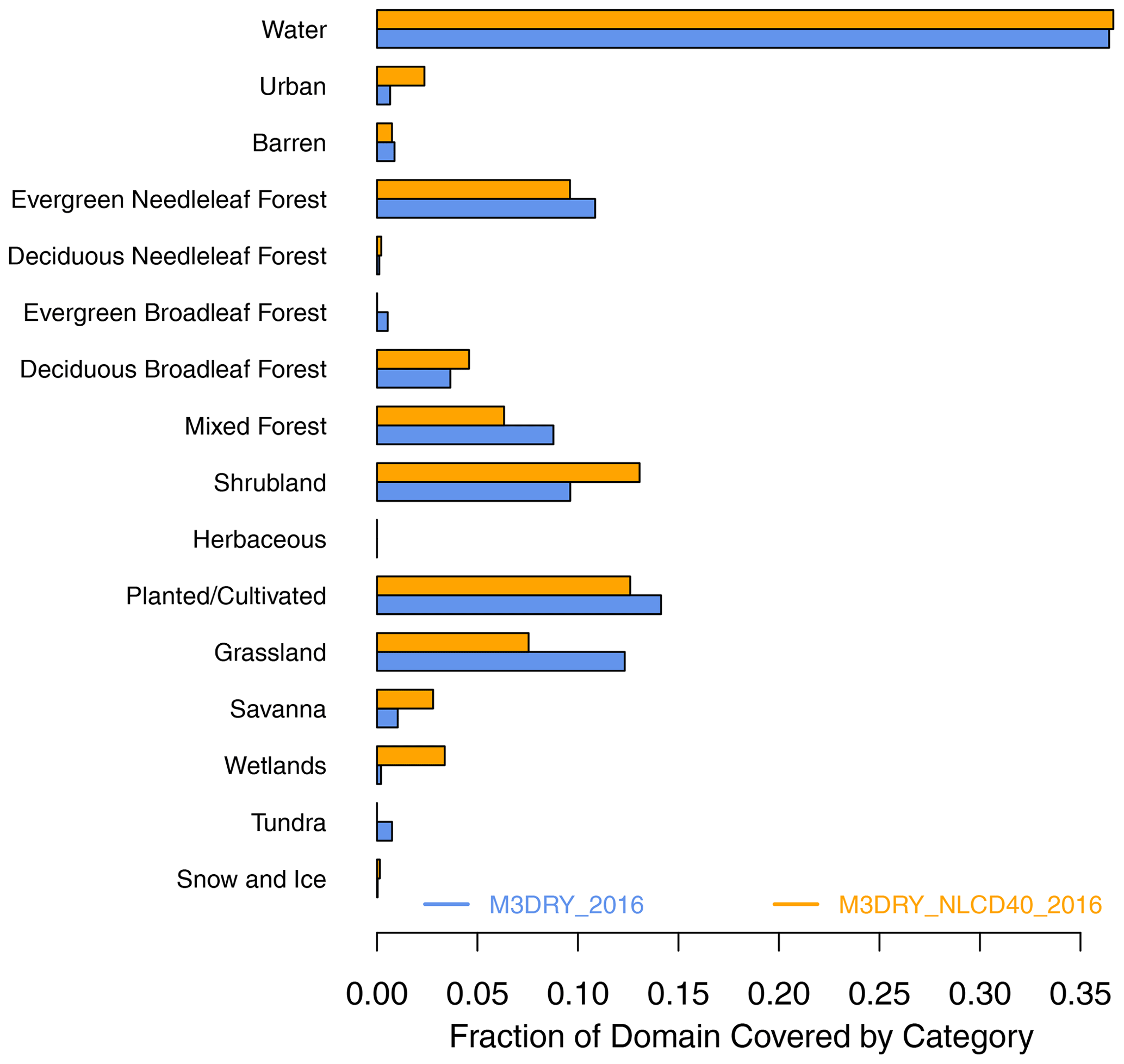
Figure 14 Domain-wide fractional coverage of the 16 AQMEII4 land-use categories (Galmarini et al., 2021) in the M3DRY_2016 (using MODIS LU in WRF PX LSM) and M3DRY_NLCD40_2016 (using NLCD40 LU in WRF PX LSM) simulations. None of the 20 MODIS land-use categories correspond to the AQMEII4 herbaceous category.

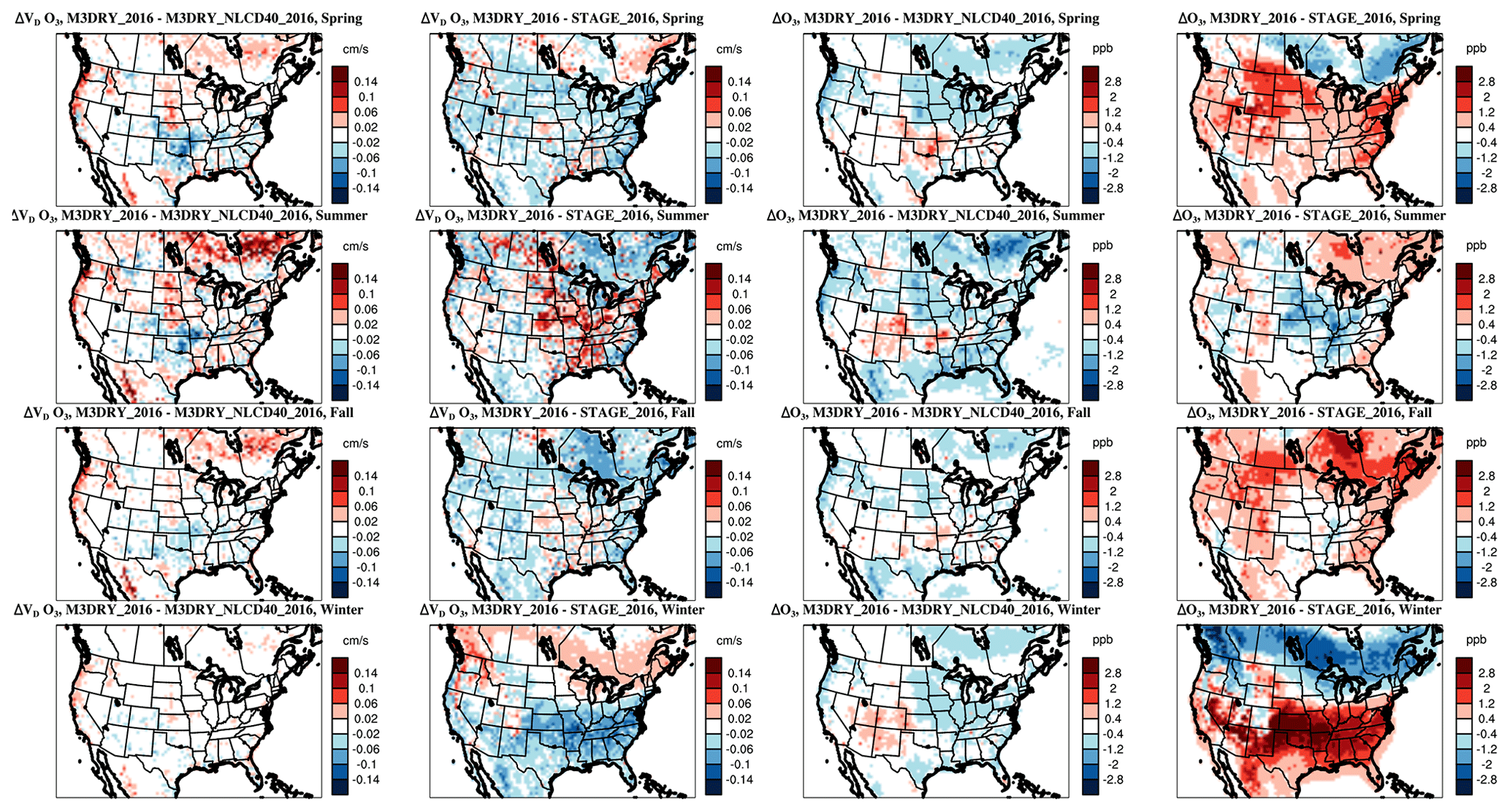
Figure 15 Differences in seasonal mean O₃ deposition velocities (columns 1 and 2) and mixing ratios (columns 3 and 4): M3DRY_2016 minus M3DRY_NLCD40_2016 (columns 1 and 3) and M3DRY_2016 minus STAGE_2016 (columns 2 and 4).

Figure 15 shows differences in seasonal mean O₃ V_d and mixing ratios between M3DRY_2016 and M3DRY_NLCD40_2016 in columns 1 and 3 to quantify the effects of using different LU schemes on these variables. Results show that the M3DRY_2016 simulation using MODIS LU tends to have higher O₃ V_d (and correspondingly lower mixing ratios) than the M3DRY_NLCD40_2016 simulation using NLCD40 LU for most seasons and regions. The differences in LU cause seasonal mean O₃ mixing ratio differences on the order of 1 ppb across large portions of the domain, with the differences generally being largest during summer and in areas characterized by the largest differences in the fractional coverages of the forest, planted and cultivated, and grassland LU categories. Columns 2 and 4 of Fig. 15 also show corresponding differences in seasonal mean O₃ V_d and mixing ratios between M3DRY_2016 and STAGE_2016 (the same data already depicted in Fig. 3) to provide a side-by-side contrast of the LU effect on these variables with the dry deposition scheme effect. While the M3Dry vs. STAGE differences are generally larger than the MODIS vs. NLCD40 differences outside the summer season, the magnitude of both effects is comparable during summer.

To assess the impacts of the LU-induced differences in V_d and mixing concentrations on effective fluxes and total dry deposition not only for O₃ but also other species, Fig. 16 shows annual total domain-wide pathway-specific dry deposition effective fluxes over all non-water grid cells for O₃, H₂O₂, HCHO, SO₂, and oxidized nitrogen species for M3DRY_2016 and M3DRY_NLCD40_2016. Note that like in equivalent Fig. 10 comparing M3DRY_2016 and STAGE_2016, O₃ dry deposition values are divided by a factor 10 to use the same y axis as for the other pollutants. Overall, the use of MODIS vs. NLCD40 results in only very minor differences in domain-total dry deposition for all species analyzed here. However, the small domain total annual differences in these grid-scale deposition fluxes likely mask larger differences existing in different regions and seasons, such as those shown for O₃ V_d and mixing ratios in Fig. 15, and differences existing for LU-specific fluxes examined below. Moreover, there is a tendency for slightly larger effective fluxes through the bare soil pathway and slightly lower effective fluxes through the cuticular and stomatal for the M3DRY_NLCD40_2016 simulation, indicating that the choice of LU datasets can result in different estimates of dry deposition fluxes through specific pathways.

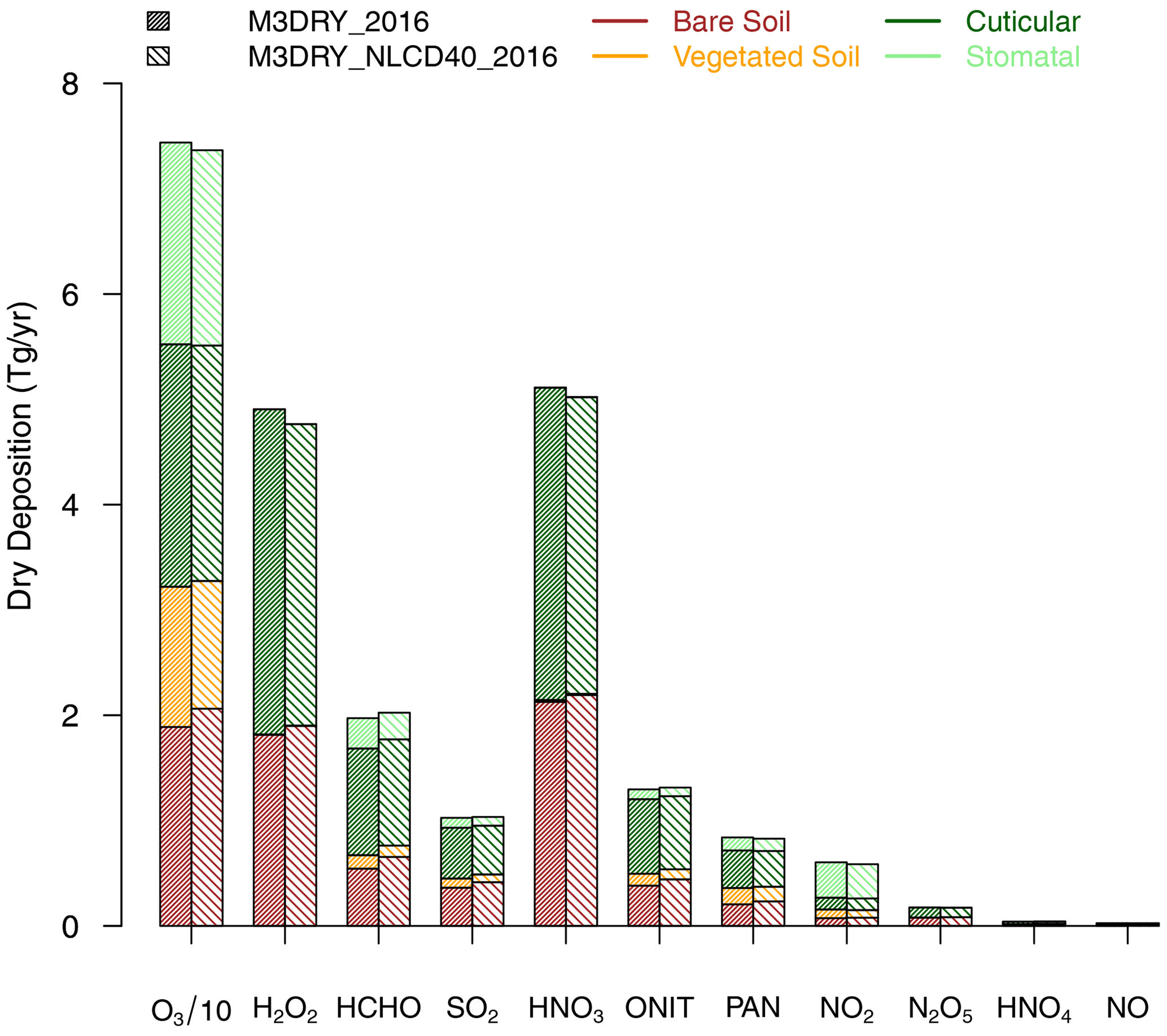
Figure 16 Grid-scale annual total domain-wide (excluding water cells) pathway-specific dry deposition fluxes (“effective fluxes”) for O₃, H₂O₂, HCHO, SO₂, and oxidized nitrogen species for M3DRY_2016 and M3DRY_NLCD40_2016. O₃ dry deposition values are divided by a factor of 10 to use the same y axis as for the other pollutants. (compare to Fig. 10).

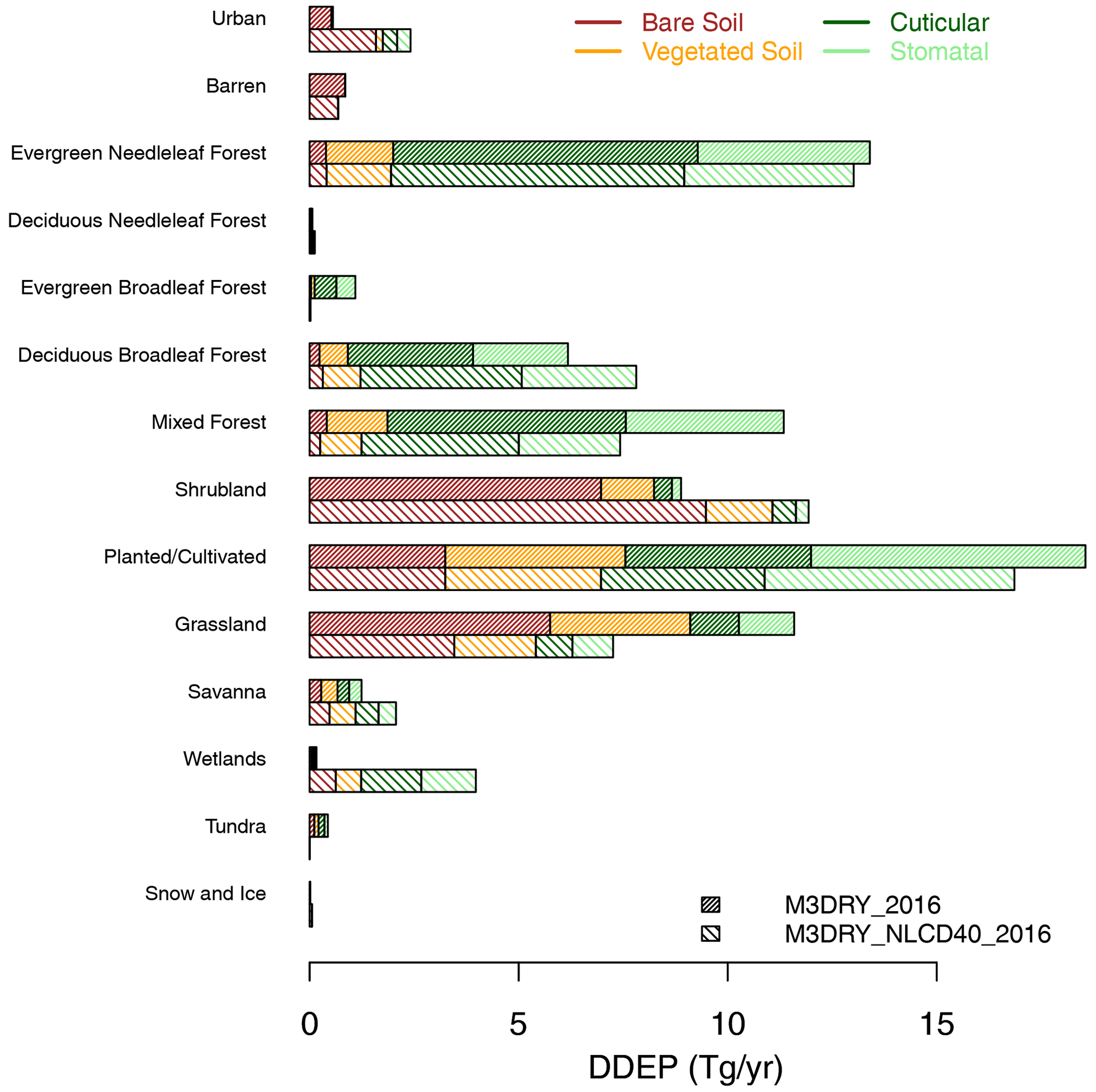
Figure 17 Land-use-specific annual total domain-wide (excluding water cells) pathway-specific O₃ dry deposition fluxes (“effective fluxes”) for M3DRY_2016 and M3DRY_NLCD40_2016. (compare to Fig. 12).

Figure 17 further disaggregates the grid-scale effective fluxes shown in Fig. 16 by LU category using O₃ as an example. Consistent with the differences in fractional coverage for the different LU categories between MODIS and NLCD40 shown in Fig. 14, domain-total O₃ deposition fluxes to the evergreen needleleaf forest, mixed forest, planted and cultivated, and grassland categories are higher for M3DRY_2016 than M3DRY_NLCD40_2016, while the opposite is the case for the urban, deciduous broadleaf forest, shrubland, savanna, and wetlands categories. For example, the fraction of the modeling domain classified as urban is 1 % for MODIS and 2.4 % for NLCD40, resulting in higher deposition estimates for this category in the M3DRY_NLCD40_2016 simulations. Moreover, because of the higher underlying spatial resolution of the NLCD satellite data and the inclusion of lower-density developed areas characterized by more vegetation in the urban LU category, this category has higher estimated effective fluxes through the stomatal and cuticular pathways in the M3DRY_NLCD40_2016 simulations compared to the M3DRY_2016 simulations. Overall, this demonstrates that the deposition impacts of LU differences are caused both by differences in the fractional coverages and spatial distributions of different LU categories and their characterization in terms of variables like VEGF and z₀ in WRF PX LSM lookup tables, which are partially tied to the spatial resolution of the underlying satellite datasets.

4 Summary and discussion

The model evaluation results presented in Sect. 3.1 demonstrate that the AQMEII4 CMAQ simulations perform similarly to other comparable regional-scale modeling studies (Emery et al., 2017; Kelly et al., 2019; Simon et al., 2012; Appel et al., 2021). The analysis of several sensitivity simulations presented in the Supplement indicates that the choice of lateral boundary conditions was the largest driver of differences in mean model concentrations and biases compared to the corresponding CMAQv5.3.1 simulations analyzed in Appel et al. (2021). Moreover, the results also indicate that while the choice of the M3Dry vs. STAGE dry deposition option can impact CMAQ performance, these impacts tend to be smaller than those caused by choices regarding model input datasets and particularly boundary conditions to represent the large-scale chemical environment.

The analysis of O₃ V_d and mixing ratios showed that during summer M3Dry has higher V_d and lower mixing ratios than STAGE for much of the eastern US, whereas the reverse is the case over eastern Canada and along the US West Coast. In contrast, during winter STAGE has higher V_d and lower mixing ratios than M3Dry over most of the southern half of the modeling domain, while the reverse is the case for much of the northern US and southern Canada. The differences in seasonal mean mixing ratios reach 2–3 ppb in a number of locations, indicating that the effects of different dry deposition schemes can be more pronounced locally than in the spatially aggregated model evaluation metrics presented in Sect. 3.1. Absolute differences in seasonal mean O₃ V_d are on the order of 0.05–0.1 cm s⁻¹ for many locations. While these differences tend to be smaller than the range of model differences reported in intercomparison studies performed at flux measurement sites (e.g., Wu et al., 2018; Clifton et al., 2023) and for global models (Hardacre et al., 2015), their magnitude nevertheless represents a variation of about 10 %–30 % in CMAQ-simulated seasonal mean V_d, with the highest relative differences generally occurring during winter.

When using grid-scale effective conductances to further analyze the differences in O₃ V_d, the comparison between M3Dry and STAGE showed generally higher summertime stomatal and wintertime cuticular effective conductances for M3Dry and generally higher soil effective conductances (both vegetated and bare) for STAGE in both summer and winter. On a domain-wide basis, the stomatal effective conductance accounted for about half of the total O₃ V_d during daytime hours in summer for both schemes, although regional variations in these contributions exist due to variations in vegetation coverage. Examining grid-scale component resistances for O₃ shows that values for summertime $\mathrm{1}/R_{\mathrm{s}}$ and wintertime $\mathrm{1}/R_{\mathrm{cut}}$ differ between M3Dry and STAGE, with the higher values of these inverted resistances in M3Dry causing higher effective conductances for these pathways compared to STAGE. Extending the concept of effective conductances to effective fluxes, annual domain total O₃ dry deposition flux results show the larger contributions from the vegetated and bare soil pathways for STAGE and the larger contributions from the stomatal and cuticular pathways for M3Dry.

In contrast to O₃, most other pollutants show larger effective conductances and effective fluxes for the bare soil and sum of bare and vegetated soil pathways for M3Dry than STAGE. The cuticular effective flux is larger for M3Dry than STAGE for HCHO, SO₂, HNO₄, and organic nitrates; smaller for M3Dry than STAGE for H₂O₂ and HNO₃; and similar between M3Dry and STAGE for other species. Stomatal effective fluxes are small for all species except O₃, HCHO, and SO₂ for both M3Dry and STAGE. Domain-wide annual total dry deposition fluxes differ the most between M3Dry and STAGE for HCHO and organic nitrate.

Extending the analysis of grid-scale dry deposition diagnostics further to specific LU categories, results show that total V_d during daytime varies by a factor of 2 between the LU categories with the lowest values (urban, barren, and snow and ice) and those with the highest values (evergreen needleleaf and broadleaf forest, deciduous forest). Effective conductances for the bare soil pathway dominate for the urban, barren, and shrubland LU categories, while conductances for the cuticular and stomatal pathways dominate for the forest LU categories, especially during daytime. Results also show that the M3Dry vs. STAGE differences are most pronounced for the stomatal and vegetated soil pathway for the forest LU categories, with M3Dry estimating larger effective conductances for the stomatal pathway and STAGE estimating larger effective conductances for the vegetated soil pathway for these LU categories. Higher effective conductances for the bare soil pathway in STAGE are particularly noticeable for the urban, shrubland, and tundra LU categories. For annual total deposition, the overall slightly larger grid-scale O₃ deposition flux for STAGE is present for almost all LU categories. Considering effective fluxes for summertime only, the greater importance of the cuticular and stomatal pathways during this season for LU categories most strongly affected by seasonal variations in LAI, along with the greater importance of these pathways in M3Dry compared to STAGE, yield greater overall estimated deposition to these LU categories for M3Dry compared to STAGE. Additional analysis showed that minor differences in LU-specific lookup table values between different deposition schemes as well as the aggregation of the MODIS LU categories to the AQMEII4 LU categories in the STAGE deposition calculations can also contribute to differences in the estimated V_d and resulting mixing ratios. Overall, the analysis of LU-specific diagnostic variables for both the entire year and summer only revealed that even though annual total O₃ deposition fluxes estimated by M3Dry and STAGE are fairly similar, pathway-specific fluxes to individual LU types can vary more substantially on both annual and seasonal scales, which is likely to affect estimates of O₃ damages to sensitive vegetation.

A comparison of two simulations differing only in their LU classification scheme (MODIS vs. NLCD40) showed that the differences in LU cause seasonal mean O₃ mixing ratio differences on the order of 1 ppb across large portions of the domain, with the differences generally largest during summer and in areas characterized by the largest differences in the fractional coverages of the forest, planted and cultivated, and grassland LU categories. These differences are generally smaller than the M3Dry vs. STAGE differences outside the summer season but have a similar magnitude during summer. When considering LU-specific effective fluxes for both simulations, results show that domain-total O₃ deposition fluxes to the evergreen needleleaf forest, mixed forest, planted and cultivated, and grassland categories are higher for the simulation using MODIS LU than the simulation using NLCD40 LU, while the opposite is the case for the urban, deciduous broadleaf forest, shrubland, savanna, and wetlands categories. Moreover, because of the higher underlying spatial resolution of the NLCD satellite data and the inclusion of lower-density developed areas characterized by more vegetation in the urban LU category, this category has higher estimated effective fluxes through the stomatal and cuticular pathways in the M3DRY_NLCD40_2016 simulated compared to the M3DRY_2016 simulations. Results indicate that the deposition impacts of LU differences are caused by differences in the fractional coverages and spatial distributions of different LU categories and their characterization in terms of variables like VEGF and z₀ in the lookup tables used in the LSM and deposition scheme.

Refining the representation of dry deposition in regional modeling systems is an area of ongoing research, leveraging new insights from observational datasets, field-scale modeling, and model intercomparisons such as those performed in AQMEII4 (Galmarini et al., 2021; Clifton et al., 2023). For example, both the M3Dry and STAGE deposition schemes in CMAQ have updated the representation of aerosol dry deposition in the recent release of CMAQv5.4 in October 2022 (U.S. Environmental Protection Agency, 2022; Pleim et al., 2022), while STAGE has also been revised to normalize R_a, R_s, and u_* to grid-scale values from the LSM used in the driving meteorological model. The analyses and results presented in this study serve as an example of how the diagnostic grid-scale and LU-specific dry deposition variables adopted for AQMEII4 can provide insights into a key model process affecting simulated pollutant budgets and ecosystem impacts of atmospheric pollution. Initial analysis of results from all AQMEII4 grid model simulations show that the differences in simulated O₃ V_d, deposition pathways, and deposition fluxes between the CMAQ M3Dry and STAGE simulations analyzed in this study tend to be smaller than the differences relative to other AQMEII4 grid models. It is expected that the forthcoming diagnostic analyses of results from all AQMEII4 grid models as well as a potentially more widespread adoption of such diagnostic variables in other modeling studies will serve the modeling community in their future development efforts. Additionally, it is hoped that the ongoing point intercomparison of the M3Dry and STAGE schemes implemented in CMAQ with schemes implemented in other models (Clifton et al., 2023), along with planned point model simulations to quantify the sensitivity of specific resistances and conductances in different schemes towards individual meteorological, soil, and biophysical forcing variables can help guide future model development efforts.