the Creative Commons Attribution 4.0 License.
the Creative Commons Attribution 4.0 License.
 | 22 May 2023
HUB: a method to model and extract the distribution of ice nucleation temperatures from drop-freezing experiments
Ingrid de Almeida Ribeiro
Konrad Meister
Valeria Molinero
The heterogeneous nucleation of ice is an important atmospheric process facilitated by a wide range of aerosols. Drop-freezing experiments are key for the determination of the ice nucleation activity of biotic and abiotic ice nucleators (INs). The results of these experiments are reported as the fraction of frozen droplets fice(T) as a function of decreasing temperature and the corresponding cumulative freezing spectra Nm(T) computed using Gabor Vali's methodology. The differential freezing spectrum nm(T) is an approximant to the underlying distribution of heterogeneous ice nucleation temperatures Pu(T) that represents the characteristic freezing temperatures of all INs in the sample. However, Nm(T) can be noisy, resulting in a differential form nm(T) that is challenging to interpret. Furthermore, there is no rigorous statistical analysis of how many droplets and dilutions are needed to obtain a well-converged nm(T) that represents the underlying distribution Pu(T). Here, we present the HUB (heterogeneous underlying-based) method and associated Python codes that model (HUB-forward code) and interpret (HUB-backward code) the results of drop-freezing experiments. HUB-forward predicts fice(T) and Nm(T) from a proposed distribution Pu(T) of IN temperatures, allowing its users to test hypotheses regarding the role of subpopulations of nuclei in freezing spectra and providing a guide for a more efficient collection of freezing data. HUB-backward uses a stochastic optimization method to compute nm(T) from either Nm(T) or fice(T). The differential spectrum computed with HUB-backward is an analytical function that can be used to reveal and characterize the underlying number of IN subpopulations of complex biological samples (e.g., ice-nucleating bacteria, fungi, pollen) and to quantify the dependence of these subpopulations on environmental variables. By delivering a way to compute the differential spectrum from drop-freezing data, and vice versa, the HUB-forward and HUB-backward codes provide a hub to connect experiments and interpretative physical quantities that can be analyzed with kinetic models and nucleation theory.
- Article
(5728 KB) - Full-text XML
-
Supplement
(1512 KB) - BibTeX
- EndNote


Ice nucleators (INs) of biological and abiotic origins present in aerosols are responsible for facilitating the heterogeneous freezing of atmospheric water droplets above the homogeneous nucleation temperature (Murray et al., 2012; DeMott et al., 2016, 2003). The potential of these aerosols as ice nuclei has significant implications for cloud properties and precipitation patterns (Gettelman et al., 2012; Mülmenstädt et al., 2015; Froyd et al., 2022). Freezing experiments are key sources of information to determine the range of temperatures over which INs promote ice nucleation. The most common method to characterize INs is through immersion freezing experiments, for which a wide range of assays and instruments have been developed. A comprehensive report of various drop-freezing techniques can be found in Miller et al. (2021). The assays are typically performed by placing uniformly sized water droplets with a known IN concentration or area on a substrate or in a multiwall plate that is gradually cooled from a temperature above 0 ∘C until all droplets are frozen (Kunert et al., 2018; Budke and Koop, 2015). Droplet freezing is detected visually or through the measurement of the latent heat release (Stratmann et al., 2004; Budke and Koop, 2015; Kunert et al., 2018; Reicher et al., 2018), allowing the assignment of a heterogeneous nucleation temperature to each droplet. Drop-freezing experiments record the fraction of frozen droplets, fice(T), as a function of decreasing temperature; for soluble or dispersible INs fice(T) curves are typically collected at various 10-fold dilutions of the IN sample.
Historically, there have been two interpretations of the dispersion of nucleation temperatures in heterogeneous freezing experiments. The first approach suggests that the stochastic nature of the nucleation process dominates the variability in freezing temperatures (Bigg, 1953; Carte, 1956), while the second approach assumes that the dispersion in temperatures mostly arises from a distribution of nucleation sites (Fletcher, 1969), each with a deterministic, singular nucleation temperature (Levine, 1950; Vali and Stansbury, 1966). Variability in the temperature, volume, and amount of ice-nucleating particles per droplet can also contribute to the dispersion of freezing temperatures (Vali, 2019; Knopf et al., 2020). There is consensus now that both stochastic effects and sample heterogeneities contribute to the distribution of freezing temperatures, and both approaches are used for the modeling of drop-freezing experiments (Vali, 1971; Marcolli et al., 2007; Niedermeier et al., 2011; Murray et al., 2011; Broadley et al., 2012; Wright and Petters, 2013; Herbert et al., 2014; Harrison et al., 2016; Alpert and Knopf, 2016; Vali, 2019; Fahy et al., 2022b). Stochastic modeling of the freezing curves is based on predicting the survival probability of liquid water containing INs as a function of supercooling, and it requires a model for the temperature dependence of the nucleation rate of the IN components. These models have been solved numerically or evolved with Monte Carlo simulations to interpret or resolve the distribution of ice nucleation properties of minerals (Marcolli et al., 2007; Murray et al., 2011; Broadley et al., 2012; Wright and Petters, 2013; Herbert et al., 2014; Harrison et al., 2016) and organics (Zobrist et al., 2007; Alpert and Knopf, 2016) and to perform parametric bootstrapping of experimental data (Wright and Petters, 2013; Harrison et al., 2016). The advantage of the stochastic modeling approach is that it enables a direct link to microscopic properties of the nuclei and can account for the cooling rate dependence of the fice(T) data. These approaches require the use of analytical models for the freezing rates and their distribution in the sample.
The modeling of freezing experiments based on the singular approach is based on the framework proposed by Vali (1971). He assumed that each particular IN has a characteristic ice nucleation temperature that is independent of the cooling history. This implies that the IN with the highest characteristic nucleation temperature in a droplet is responsible for its freezing. Given a total number of droplets N0, the number of frozen droplets NF(T) at a temperature T gives the range of characteristic freezing temperatures that determines the ice nucleation activity and is used to produce the cumulative freezing spectrum (Vali, 1971, 2014, 2019):
where is the number of unfrozen droplets; is the fraction of frozen droplets at temperature T; and X is a normalization factor per unit volume of water, unit mass, or surface of the INs (Vali, 2019). For soluble INs, the normalization factor is commonly defined by the mass of the ice-nucleating material , where ρ is the density of the initial solution, Vdrop is the droplet volume, and d is the dilution factor (Kunert et al., 2018). The IN surface area per drop, X=Adrop, is sometimes used as the normalization factor for insoluble INs (e.g., dust, crystals), resulting in a cumulative spectrum per area denoted as Ns(T). However, it is challenging to measure the total IN surface area accurately (Knopf et al., 2020). We note that Eq. (1a) can be used even when the absolute concentrations or areas of the INs are unknown, provided that the user knows the relative concentration of the dilution series derived from a parent sample. The differential freezing spectrum nm(T) is obtained by the differentiation of the cumulative spectrum (Vali, 1971):
The differential spectrum identifies the density of IN active at each temperature and was identified by Vali as the central quantity that can be derived and interpreted from drop-freezing experiments (Vali, 1971, 2019).
The determination of the differential spectrum from the cumulative one by finite differentiation is subject to significant noise, requiring a careful selection of the temperature intervals and extensive sampling (Vali, 2019). As stochastic effects are not considered in the singular temperature formalism, the cumulative and differential spectra should – in principle – depend on the cooling rate (Vali, 1994). The stochastic nature of ice nucleation, combined with the uncertainties associated with the experimental measurements (e.g., different droplet volumes, inhomogeneous samples, different detection efficiencies), can produce significant variations in the cumulative freezing spectra that result in large uncertainties in nm(T) and we provide its associated Python code and user manual (https://github.com/Molinero-Group/underlying-distribution, last access: 5 May 2023), published in de Almeida Ribeiro et al., 2023). Parametric and nonparametric bootstrapping based on the singular approximation and Monte Carlo simulations have been used to estimate confidence intervals in freezing spectrum measurements (Vali, 2019; Fahy et al., 2022a, b).
A central assumption of the singular freezing approximation is that the freezing of a droplet containing multiple INs is promoted by the IN with the highest nucleation temperature (Levine, 1950). The extreme value sampling is apparent in the concentration dependence of fice(T) in experiments (Marcolli et al., 2007; Budke and Koop, 2015; Kunert et al., 2018; Lukas et al., 2022). Using probability theory, Joseph Levine demonstrated that if the distribution of ice nucleation temperatures of the IN population follows an exponential distribution, then the sampling of droplet freezing temperatures corresponds to a Gumbel distribution, and the median freezing temperature TMED of the droplets scales with the logarithm of the number (or total nucleating area) of IN per droplet (Levine, 1950). Richard Sear more recently demonstrated that Levine's approach is a particular solution for a generalized extreme value problem and used modern extreme value statistics to derive the scaling of TMED with the number of IN sites per droplet for the three generalized extreme value (GEV) distributions: Gumbel that would arise from an underlying IN distribution with exponential tails, Frechet from those with power law tails, and Weibull from those with an upper cutoff in the freezing temperature of the INs (Sear, 2013). However, there are limitations for the use of the analytical approaches of Sear and Levine for the interpretation of actual drop-freezing data. First, the extreme value sampling results in one of the three GEV distributions only in the limit of an extremely large number of INs per droplet, while in experiments the sampling is typically performed over dilutions down to a few INs per droplet. There is no analytical formulation for the dependence of the extreme value distribution in the low to intermediate concentration regime. Second, the analytical theory assumes that the sampling is complete (i.e., the number of droplets is extremely large), while experiments are typically performed with tens to hundreds of droplets. Third, Sear notes that there is no general analytical theory to predict the GEV distributions from a mixture of populations of nuclei with different temperature dependences (Sear, 2013). In this study we overcome these three limitations through a numerical implementation of extreme value statistics for the modeling of drop-freezing experiments.
A consequence of extreme value sampling is that the differential spectrum nm(T) represents the underlying distribution of ice nucleation temperatures of all INs in the sample, which we denote as Pu(T), only when the sampling of INs in the drop-freezing experiments is complete. The underlying distribution Pu(T) is akin to a hub that connects the experimental freezing temperatures to physical analysis based on nucleation theory or kinetic and equilibrium models that can elucidate the mechanisms and origins of the distributions of INs (Fig. 1). We here call the cumulative spectrum Nm(T) obtained through Eq. (1a) in this complete sampling limit the intrinsic cumulative spectrum of the system, Iu(T) (Fig. 1). While there is consensus that the quality of the freezing spectrum increases with the number of droplets, a rigorous analysis of how many droplets and IN dilutions should be measured to provide accurate freezing spectra is still lacking. The first goal of the present study is to provide a strategy to optimize the sampling of drop-freezing experiments to derive interpretable differential spectra that are a good approximant of the underlying distribution of heterogeneous ice nucleation temperatures of the sample.
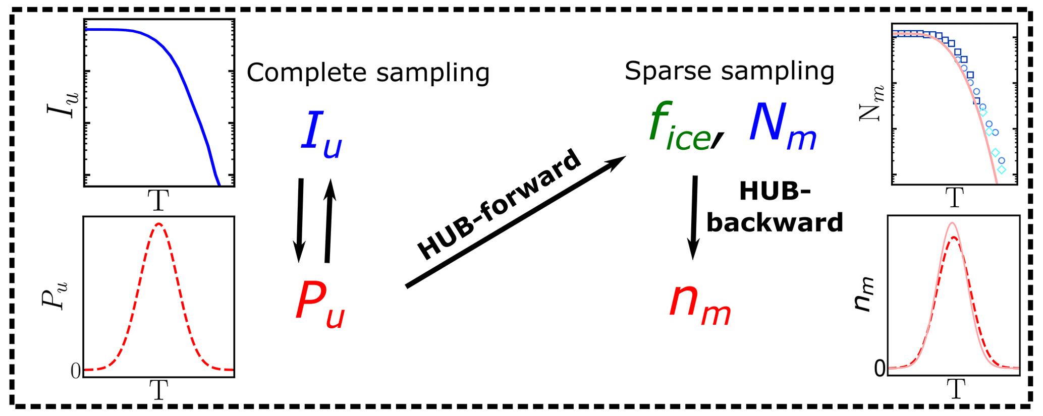
Figure 1Diagram illustrating the usage of the HUB code: nm(T) is obtained from the sparsely sampled fice(T) or Nm(T) through HUB-backward, and the effect on fice(T) or Nm(T) is obtained from the complete sampling of the underlying distribution Pu(T) through HUB-forward. The intrinsic cumulative spectrum Iu(T) is proportional to (Sect. 2.2).
The existence of subpopulations or classes in the population of INs (e.g., different classes of bacterial INs, different ice-nucleating sites on complex materials like dust) (Turner et al., 1990) is common in atmospheric aerosols. While several studies have broadly defined populations from the cumulative spectra by the range of nucleation temperatures they encompass (Turner et al., 1990; Creamean et al., 2019) or the origin of the sample (Steinke et al., 2020), there is currently no simple procedure to identify and quantify subpopulations or classes from cumulative freezing spectra Nm(T). The second aim of our study is to map the cumulative freezing spectrum Nm(T) into the differential spectrum nm(T) in terms of subpopulations that may correspond to different physical nucleation sites in the sample.
To reach the aims above, we develop a method we name HUB (for heterogeneous underlying-based) to model and interpret the results of drop-freezing experiments and provide its associated Python code and user manual (https://github.com/Molinero-Group/underlying-distribution, last access: 5 May 2023). Our method relies on the singular interpretation of freezing experiments: we assume that each individual IN has a characteristic nucleation temperature independent of its cooling history and that the freezing of a droplet containing multiple INs is promoted by the IN with the highest nucleation temperature. This second assumption allows the use of extreme value statistics (Castillo et al., 2005; David and Nagaraja, 2004; Gumbel, 2012; De Haan and Ferreira, 2006) to model and interpret the data.
We present two implementations of the HUB analysis code. The HUB-forward code allows the user to postulate an underlying distribution of heterogeneous nucleation temperatures Pu(T) in the system of interest. The HUB-forward code uses the singular approximation and extreme value statistics to generate an artificial IN dilution series similar to those obtained in experiments, from which it computes the fraction of frozen droplets fice(T) and from these derive Nm(T) using Vali's equation (Fig. 1). The HUB-backward code works in reverse, extracting the differential spectrum nm(T) from a given cumulative Nm(T) using a stochastic optimization procedure (Fig. 1). HUB-backward allows the decomposition of the total population from nm(T) into subpopulations. The combination of HUB-forward and HUB-backward allows for an analysis of the sensitivity of Nm(T) to the number of droplets and dilutions, as well as the impact of the sampling on the closeness of the differential spectrum nm(T) to the underlying distribution Pu(T). The determination of distributions obtained from the HUB-backward code could further enable the interpretation of the experimental ice nucleation spectra with the size and structure of INs using nucleation theory, kinetic models, and molecular simulations. For example, Schwidetzky et al. (2023) illustrate the use of the distribution of freezing temperatures obtained with HUB-backward, together with classical nucleation theory for finite surfaces, to interpret the size of the INs of Fusarium acuminatum.
This paper is organized as follows: Sect. 2 presents the methodology, and Sect. 2.1 discusses the details on the implementation of HUB-forward, while Sect. 2.2 describes the HUB-backward procedure to find the differential spectrum nm(T) and discusses how to determine whether or not nm(T) has converged to the underlying distribution Pu(T). Section 3 presents examples of applications of both HUB-forward and HUB-backward codes and their capabilities. Section 3.1 analyses the effect of the number of droplets sampled on the cumulative freezing spectrum Nm(T). Section 3.2 uses HUB-backward to compute the differential spectra nm(T) of various biological INs with increasing grades of complexity in their cumulative freezing spectra. Section 3.3 demonstrates how to extract nm(T) from the experimental fraction of ice fice(T) and the impact of the cooling rate on nm(T). We end in Sect. 4 with a discussion of the main conclusions and outlook.
2.1 HUB-forward method to compute the fraction of frozen droplets fice(T) and cumulative freezing spectrum Nm(T) from a known underlying distribution Pu(T)
In the HUB-forward analysis we know or assume an underlying distribution Pu(T) of ice nucleation temperatures for the IN in the sample and generate from it an artificial IN dilution series similar to those obtained in experiments, from which we compute the cumulative freezing spectrum Nm(T) using Vali's equation (Eq. 1a). Using this approach, we investigate the relationship between Nm(T) and Pu(T) (Fig. 1) and the sensitivity of Nm(T) with respect to the number of droplets and dilutions. For generality, we represent Pu(T) as a linear combination of normalized continuous distributions Pi(T) that represent subpopulations of freezing temperatures:
where p is the total number of subpopulations, are normalized distribution functions, and c1, c2, …, cp are their weights such that . These subpopulations could correspond to different chemical, topographical, or structural motifs in the IN samples, although chemically distinct species could also produce overlapped freezing signatures, and a single species could display a broad freezing range. Our formalism does not require a mapping of subpopulations of freezing temperatures to physical IN sites. The units of Pu(T) are the same as for nm(T), i.e., those of the cumulative spectrum divided by a unit of temperature, but are generally omitted in what follows. Throughout this work we assume that Pi(T) can be represented by Gaussian (i.e., normal) distributions:
where each subpopulation Pi(T) is further characterized by its most likely temperature of freezing Tmode,i and spread of distribution of freezing temperatures si. We also provide in the HUB code the option for the user to use the log-normal distribution, which has a tail towards higher temperatures, or the left-tailed Gumbel distribution, which has a tail towards lower temperatures. In our model, we assume that the underlying distribution of ice-nucleating temperatures Pu(T) does not change with the concentration of INs. This last condition is violated when INs are involved in chemical, aggregation, or solubility equilibria that alter the proportionality between their concentration and the dilution factor of the sample, resulting in a lack of overlap of the pieces of the cumulative spectra Nm(T) obtained from different dilutions (Bogler and Borduas-Dedekind, 2020).
The number of INs in each droplet is given by the Poisson distribution:
where n is the actual number of INs in each droplet and λ represents the average number of INs among all droplets of the corresponding dilution. Figure 2a shows the probability mass function (PMF) for λ=1, 5, and 10, computed according to Eq. (4) and sampling over N0=104 droplets using the “SciPy Stats” Python framework (Virtanen et al., 2020). As λ increases, the probability that any droplet nucleates homogeneously rapidly approaches zero (inset of Fig. 2a). When there is one IN on average per droplet % of the droplets do not have any INs; i.e., they are “empty” droplets that would nucleate at the homogeneous nucleation temperature. We note that by performing dilutions until a sizeable fraction of droplets nucleate homogeneously, it is possible to calibrate the absolute concentration of ice nuclei in the original, undiluted sample.
To illustrate how the heterogeneous ice nucleation temperatures recorded in drop-freezing experiments depend on the number of INs in the droplets, we start from two examples with Pu(T) represented by one or two Gaussian subpopulations, shown with dashed black lines in Fig. 2b and c, respectively. We assign a temperature to each IN contained in droplets from a 10-fold dilution series of five solutions with λ=1, 10, 102, 103, and 104 average number of INs per droplet. If the droplet volume is constant, λ is proportional to the concentration of INs in the droplets. We sample N0=104 droplets for each concentration. This N0 is much higher than the ∼100 droplets usually sampled in laboratory experiments; we address the effect of sampling in Sect. 3.1 below.
To sample independent random values for each IN, the number of random variates, which are drawn from Pu(T), is the total number of INs among N0 droplets. Thereby, each droplet has a set of temperatures , where j is the droplet index and k is the IN index. Since we assume that freezing occurs at the characteristic temperature of the IN with the highest freezing temperature, the nucleation temperature for each droplet is defined as the maximum, i.e., the extreme upper value, of several independent freezing temperatures . Figure 2b and c show the normalized distribution of for different values of λ, namely . Therefore, Pu(T) represents the underlying probability of heterogeneous ice nucleation temperatures independent of the concentration of INs, while represents the concentration-dependent distribution and has the same units as Pu(T) and the differential spectrum. According to the Fisher–Tippett–Gnedenko theorem, the distribution of extreme upper values of the Gaussian distribution is the right-skewed Gumbel distribution (Castillo et al., 2005; David and Nagaraja, 2004; Gumbel, 2012; De Haan and Ferreira, 2006), which has a fatter tail on the high-temperature side of its maximum. Indeed, the shift in curves in Fig. 1b and c evinces that as the number of INs in the droplet increases, the probability of sampling the higher temperature tail of Pu(T) increases significantly. This skew is the reason why several dilutions are needed to sample the full population of ice nucleants.
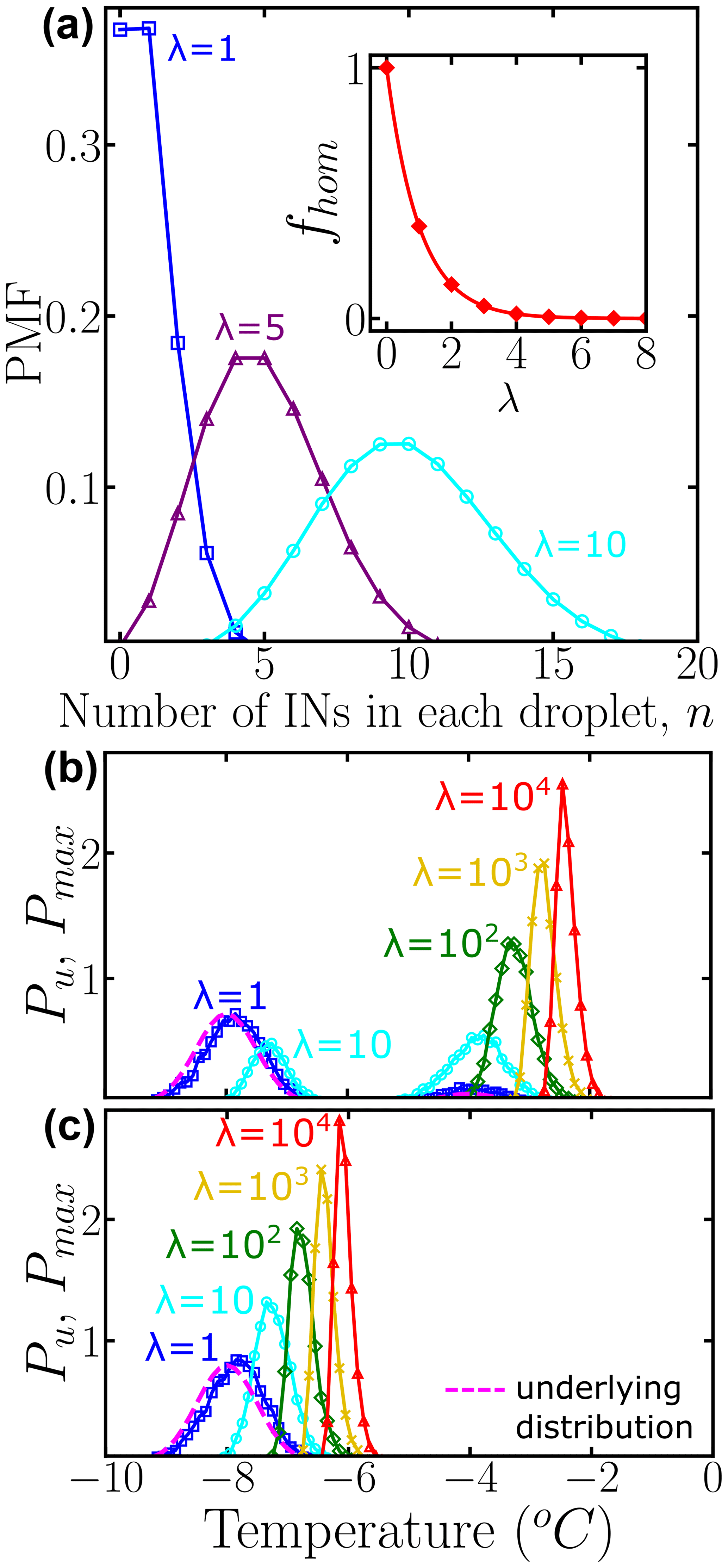
Figure 2(a) Probability mass function (PMF) of the Poisson distribution representing the number of INs per droplet. Colors represent different average numbers of INs per droplet: λ=1 (blue squares), λ=5 (purple triangles), and λ=10 (cyan circles). The inset shows the fraction of empty droplets as a function of λ. The connecting lines are solely guides for the eye. Panels (b) and (c) show the normalized underlying distributions Pu(T) of heterogeneous ice nucleation temperatures (dashed magenta line), composed of two subpopulations and one subpopulation, respectively. Colors represent the concentration-dependent normalized distribution of heterogeneous ice nucleation temperatures: λ=1 (blue squares), λ=10 (cyan circles), λ=102 (green diamonds), λ=103 (yellow ×), and λ=104 (red triangles) INs per droplet. A bin width of 0.1 was used for Pu(T) and . All distributions were obtained using 104 droplets. While the HUB-forward code explicitly accounts for and N0, we note that their ratio can be approximated by based on properties of the Poisson distribution.
HUB-forward computes the fraction of frozen droplets and cumulative spectra from a proposed underlying distribution of freezing temperatures, using extreme value statistics. The fraction of frozen droplets can be calculated as a function of the concentration-dependent distribution:
where the integration is from the ice melting temperature Tm to the temperature is the total number of droplets that freeze heterogeneously, and N0 is the total number of droplets. We note that the approach taken in this work differs from that of previous studies that start from a microscopic model for the nucleation sites and nucleation theory to predict the fraction of frozen droplets using Monte Carlo simulations, as well as from previous modeling using the singular approximation, which do not account for the statistics of extreme sampling.
To use the HUB-forward code, the user must define the total number of droplets “ndroplets” that serves as the total number of each concentration and the number of subpopulations “nsubpop”. If “nsubpop” = 1, the user must provide the temperature of maximum likelihood Tmode,1 and the spread s1. If “nsubpop” = 2, the user must provide Tmode,1, s1, Tmode,2, s2 and c2. If “nsubpop” = 3, the user has to provide Tmode,1, s1, Tmode,2, s2, c2, and Tmode,3, s3, c3. To generate the cumulative freezing spectrum Nm(T), the user needs to define the total number of concentrations “nconc”; the concentration of the parent suspension is defined in “density” and the droplet volume in “volumedrop”. The output is composed of different data plots and files: the normalized Pu(T) and , the artificially generated , and Nm(T) built from the 10-fold dilution series.
Figure 3a and b show the fraction of ice computed using of Fig. 2b and c, which correspond to Pu(T) with two subpopulations and one subpopulation, respectively. The intermediate plateau in Fig. 3b indicates that no droplets freeze at those temperatures. As discussed above, only 63 % of the droplets freeze heterogeneously for λ=1. We assume droplets of uniform volume Vdrop=0.1 µL obtained through 10-fold dilution of a parent suspension with λ=104 INs per droplet corresponding to a mass m=1 mg of IN in a volume Vwash=1 mL. We use Eq. (5) and the Pu(T) of Fig. 2b and c to generate (Fig. 3a and b), sampling either 100 or 104 droplets per dilution. We combine the using Eq. (1a) to build the cumulative freezing spectra Nm(T) shown in Fig. 3c and d (sampling 104 droplets per dilution) and Fig. 3e and f (sampling 102 droplets per dilution).

Figure 3Panels (a) and (b) represent the fraction of ice computed using Eq. (5) and artificially generated data using 104 droplets. Panels (c) and (d) are the corresponding cumulative freezing spectra Nm(T) computed using Vali's equation. Colors represent the different number of INs per droplet: λ=1 (blue squares), λ=10 (cyan circles), λ=102 (green diamonds), λ=103 (yellow ×), and λ=104 (red triangles). Panels (e) and (f) represent Nm(T) obtained using 100 droplets. The dashed black lines in (c) and (d) indicate the temperatures corresponding to the location of the mode(s) in the underlying distribution. The dotted magenta lines are the knee points computed with the Python function “kneed”.
The ability of HUB-forward to generate the cumulative freezing spectrum Nm(T) from the underlying distribution Pu(T) allows for an analysis of the sensitivity of Nm(T) and Pu(T) to the number of droplets and dilutions, as seen in the comparison of Nm(T) generated from the same underlying distributions using 100 and 104 droplets in Fig. 3. In Sect. 3.1 we show that the sampling with 100 droplets for only four dilutions of a system with two subpopulations of INs results in distortions of the distribution of freezing temperatures and the proportions of these populations in the differential spectrum.
The knee point in Nm(T) corresponds to the point of maximum curvature (Satopaa et al., 2011) and has been used to characterize the nucleation temperature of a particular subpopulation (Hartmann et al., 2022). Similar to Hartmann et al. (2022), we have identified in Fig. 3c and d the knee points (dotted magenta line) of the artificially generated Nm(T) by using a Python function named “kneed”. The Python function “kneed” using S=1, curve = “concave”, and direction = “decreasing”. The knee points Tknee are very close to the temperatures of maximum likelihood Tmode (dashed black lines) of the corresponding underlying distribution Pu(T), because under these conditions the differential freezing spectrum nm(T) is a very good approximant for Pu(T). However, we find that the removal of the more dilute solutions eliminates the plateau in Nm(T) and results in poor estimation of the modes of Pu(T) from the knee of Nm(T).
2.2 HUB-backward method to recover the differential freezing spectrum nm(T) from the cumulative freezing spectrum Nm(T) by a stochastic optimization procedure
The HUB-backward code implements a stochastic optimization procedure to extract the differential spectrum nm(T) from a given cumulative spectrum Nm(T) or from an experimental fice(T) curve. The latter is useful when data are available for a single concentration. One possibility for obtaining nm(T) from Nm(T) would be to follow the following steps: (i) propose a trial function , (ii) use HUB-forward to predict the concentration-dependent distributions for various IN concentrations, (iii) use these in Eq. (5) to predict the freezing fractions , (iv) compute from the freezing fractions using Eq. (1a), (v) evaluate the difference between that trial and the target (experimental) value using
and then (vi) evolve the parameters that determine until the difference δ(T) is minimized. However, the use of HUB-forward in steps (ii) and (iii) to generate and evaluate hundreds of droplets containing up to tens of millions of INs would require significant computations that render this optimization process inefficient.
The HUB-backward optimization procedure, sketched in Fig. 4, uses a shortcut for steps (ii) and (iii) above to directly predict from with fast convergence. The shortcut is based on the understanding that, in the asymptotic limit in which the sample is extremely dilute (i.e., λ⟶0), each droplet that nucleates heterogeneously contains a single IN. In such a case, sampling an infinitely large number of droplets with is equivalent to sampling each and every IN, i.e., . In agreement with this ansatz, Fig. 2b and c show that the underlying distribution Pu(T) (dashed black line) and the concentration-dependent (blue squares) sampled with 104 droplets per dilution are already very close, i.e., .
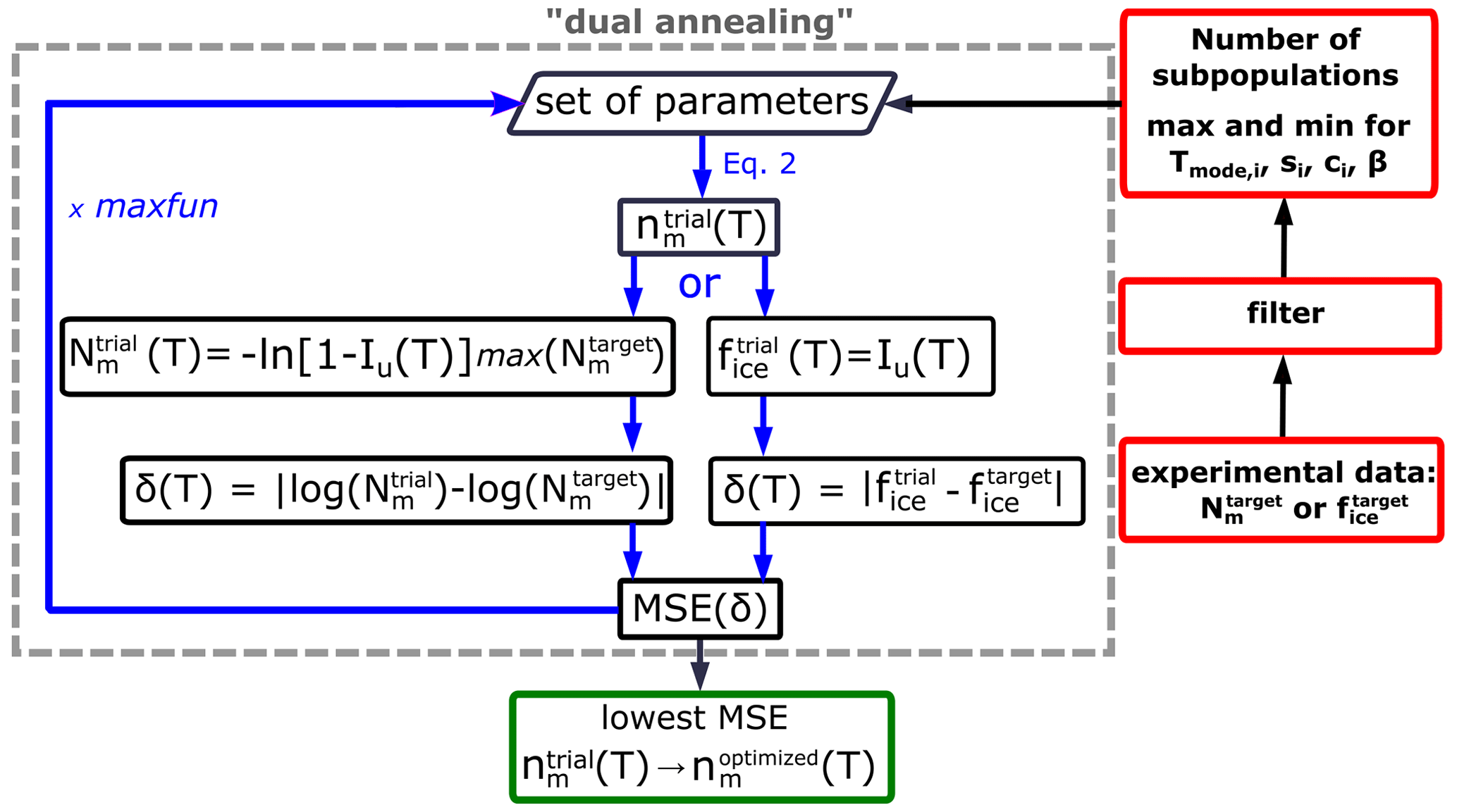
Figure 4Flowchart of the optimization procedure to obtain the differential freezing spectrum nm(T) from the full cumulative freezing spectrum Nm(T) or fraction of frozen droplets fice(T).
With this insight and considering the intrinsic cumulative spectrum, , we define the cumulative integral of the differential spectrum as
where the integration is from the ice melting temperature Tm to the temperature T and β is an adjustable scaling factor to be obtained from the optimization. Likewise, a similar estimate can be made for a single fraction of ice curve using Eq. (7) and the mean squared error can be directly evaluated (Fig. 4). When the target is a cumulative freezing spectrum, HUB-forward uses to predict a trial cumulative freezing spectrum (Fig. 4),
where corresponds to the maximum of the cumulative spectrum in the target distribution, . With Eq. (8) we obtain an that we compare with the target using Eq. (6) (Fig. 4). To do the comparison, HUB-backward uses a spline fit to interpolate the experimental , in order to have equally spaced temperature points to compare with the estimates in . We use the “interp1d” algorithm, which is available in the Python SciPy library (Virtanen et al., 2020), with a linear interpolation to construct new equally spaced data points within the range of the lowest and highest temperature values in the freezing spectrum. The cost function for the optimization is the mean squared error (MSE), computed from the difference δ(T) in Eq. (6):
where t represents the total number of equally spaced points in δ(T).
We use a stochastic global optimization technique based on a simulated annealing algorithm to find the set of parameters of (Eqs. 2 and 3) and β (Eq. 7) that globally minimize the MSE. We use the simulated annealing (SA) algorithm “dual annealing” that is part of the SciPy minimize library (Virtanen et al., 2020) with its default arguments predefined, except for the parameters “maxfun” that sets the maximum number of evaluations of the objective function (we select “maxfun” = 1 000 000 in the examples below) and the seed for the generation of random numbers (a new random integer is automatically generated every time the HUB-backward code is run). We show below that the optimized differential spectra, , are quite insensitive to the value of the seed.
The output of HUB-backward is an optimized differential spectrum or an optimized fraction of ice . To quantify how much this optimized prediction deviates from the known underlying distribution in the examples of Fig. 5, where Pu(T) is known, we define the mean relative error (MRE) for the set of parameters:
where p is the number of subpopulations.
We now turn our focus to how to select the input parameters required by HUB-backward to start the search for the underlying distribution, using the experimental or as a guide. The code requires the user to define the number of distinct Gaussian subpopulations Pi(T) that comprise the underlying distribution (Eq. 2) and to provide upper and lower bounds for the weights ci, their modes Tmode,i, and spreads si of each of these populations. In general, we find that defining the minimum and maximum values for the weights to and (see constraint in Eq. 2), for the modes and to between the homogeneous nucleation temperature (about −30 ∘C) and the melting temperature (0 ∘C), and for the spreads to ∘C and ∘C works well. However, these bounds can be tuned in order to better fit the data (as we find for pollen in Sect. 3.2 below). If the existing experimental data are very noisy, they can be interpolated in HUB-backward using the method “interp1d” with “npoints” = 100 and then smoothed with a Savitzky–Golay filter by changing the parameters “window_length”, which is the length of the filter window, and “polyorder”, which is the order of the polynomial used to fit the samples (“filter” in Fig. 4). The default values are 3 and 1, respectively. HUB-backward generates a plot that compares the original and the interpolated target data.
To identify the minimum number of subpopulations needed to represent a given freezing spectrum, we consider that every time a population is accumulated in Nm(T) or fice(T), these functions display a sharp increase. We note that assuming a large number of subpopulations may challenge the interpretability of the optimized differential spectrum .
We apply the HUB-backward procedure to the Nm(T) obtained in Fig. 3c and d by sampling four 10-fold dilutions with 100 droplets, i.e., only a total of 500 droplets. Figure 5 shows the comparison between the predicted (solid magenta lines) and the target (dashed black lines) Nm(T) (panels a and b) and nm(T) (panels c and d). Table 1 shows the predicted parameters and the precision of the optimization procedure to recover the known underlying distribution Pu(T). The MRE between the underlying distribution Pu(T) and the optimized differential spectrum is 2 % for the system with one subpopulation and 13 % for the one with two despite the low number of droplets used to sample the cumulative freezing spectra in the computer-generated freezing experiments.
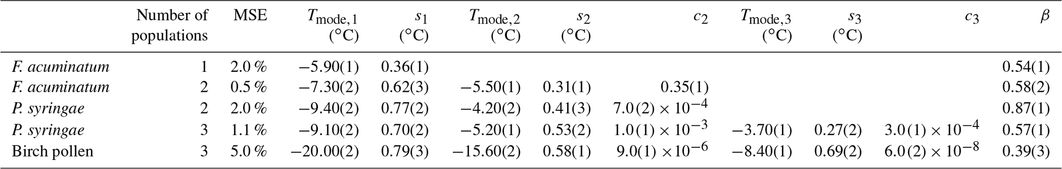
Table 1Mean relative error (MRE), mean squared error (MSE), and parameters of the optimized differential freezing spectra obtained using the HUB-backward code. The values shown here were calculated based on the average of n=3 independent runs. The error bars, shown in parentheses, were calculated by dividing the standard deviation of the values in these runs by 3.

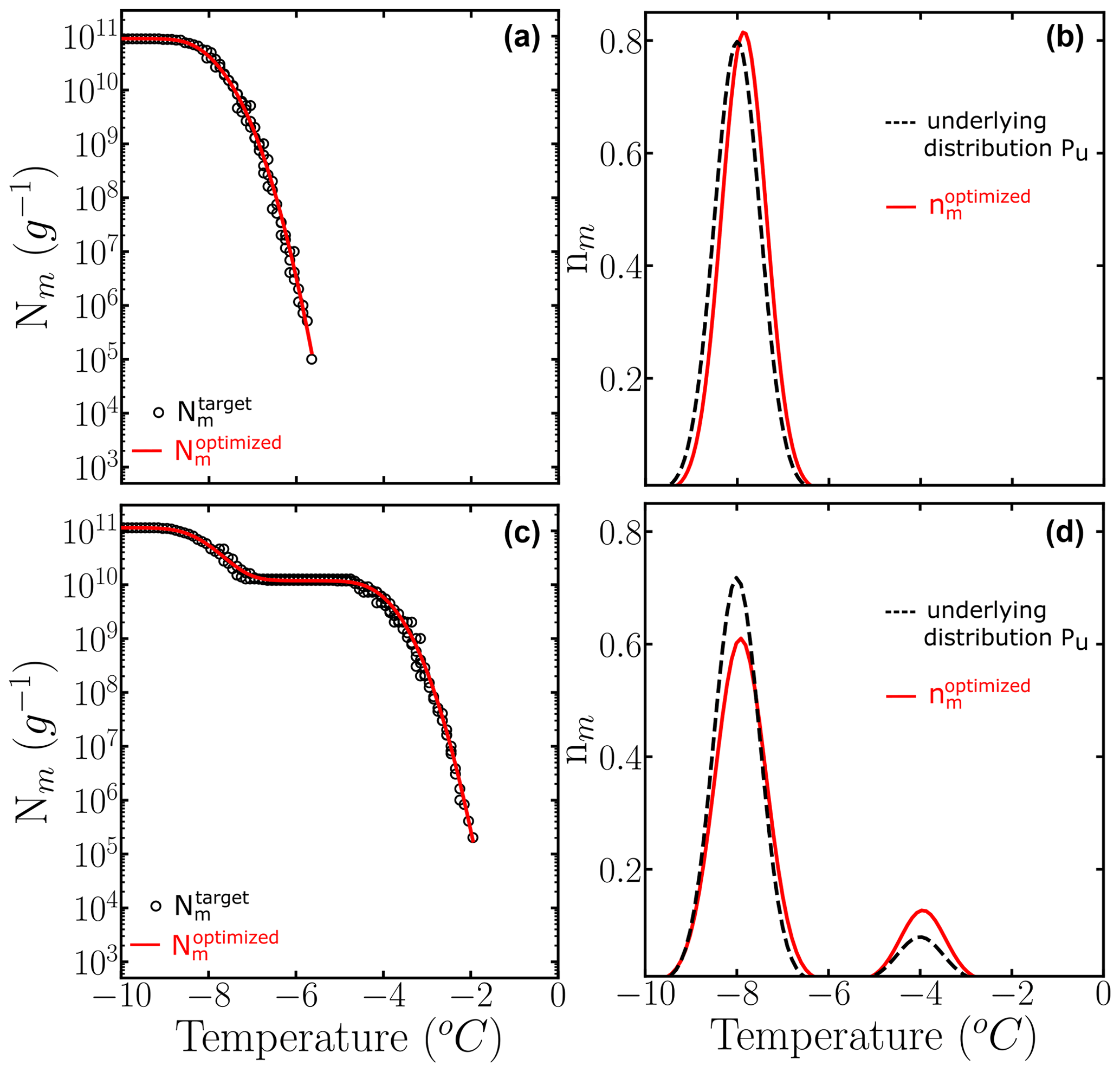
Figure 5Panels (a) and (b) show the comparison between (black circles) and the computed with the optimized solution (solid red line). Panels (c) and (d) show the known underlying distributions Pu(T) (dashed black line) and the optimized underlying distributions (solid red line) based on three independent runs. The parameters of the predicted underlying distribution are summarized in Table 1.
We conclude that the HUB-backward code gives a good estimate of the mode, spread, and weights of the populations of INs in a sample and it can be applied in a situation where Pu(T) is unknown. In Sect. 3.1 we discuss how the accuracy is of the underlying distribution recovered with HUB-backward impacted by various schemes of the sampling of the number of droplets and dilutions to construct Nm(T). In Sect. 3.2, we apply the HUB-backward procedure to obtain from actual Nm(T) of experiments with various soluble biological INs. In Sect. 3.3, we apply the HUB-backward procedure to obtain from fice(T) of experiments of insoluble crystal INs.
3.1 Effect of the number of droplets and dilutions on the cumulative freezing spectrum Nm(T)
Figure 3d–f show Nm(T) generated with HUB-forward using five dilutions from λ=104 to 1 of a solution with Pu(T) containing two populations in a ratio of 9 to 1. The Nm(T) are different when the number of droplets per dilution is 100 (Fig. 3f) or 104 (Fig. 3d). As shown in the previous section, the freezing spectrum obtained with 100 droplets and five dilutions has enough sampling to recover this Pu(T) with good accuracy (Fig. 5c and d). We test different number of droplets and concentrations, defined by the average number of INs per droplet λ, to test the sensitivity of nm(T) to the number of droplets and dilutions when the underlying distribution Pu(T) is known. We use HUB-forward to build Nm(T) based on a combination of different numbers of droplets and concentrations, similar to the case shown in Fig. 3f. Then, we use HUB-backward to obtain , compare it to Pu(T), and test the accuracy of each prediction through its mean relative error (MRE) defined in Eq. (10).
The left panels of Fig. 6 show Nm(T) generated with HUB-forward based on a combination of different concentrations using 100 droplets for each dilution. The magenta lines are based on the data provided by the HUB-backward code. The right panels of Fig. 6 compare in magenta and the known underlying distribution Pu(T) in black. In this example, nm(T) is very close to Pu(T) if both subpopulations are sampled enough. However, if the most dilute solution with λ=1 is not included in Nm(T) (second panel), the estimate of the underlying distribution is very poor. Thus, to improve the sampling of the lower tail of Pu(T), we recommend ending the dilution series always in the immediacy of λ=1, which can be gleaned from the temperature range for which Nm(T) becomes flat and a sizeable fraction of droplets of the more diluted sample nucleates homogeneously (inset of Fig. 2a). The one-to-one correspondence between the fraction of droplets nucleated homogeneously and the average number of particles in the droplet in the highly diluted limit (inset of Fig. 2a) demonstrates that reaching this limit allows for an absolute calibration of the number of INs in the initial sample. Moreover, sampling to concentrations down to about one nucleant per droplet is essential to recover a proper weight of the poorly nucleating IN populations.

Figure 6Panels (a, c, e, g) represent the cumulative freezing spectra Nm(T) sampled from the same underlying distribution Pu(T). Colors represent the different numbers of INs per droplet: λ=1 (blue squares), λ=10 (cyan circles), λ=102 (green diamonds), λ=103 (yellow ×), and λ=104 (red triangles). The sampling was done using 100 droplets for each concentration. Panels (b, d, f, h) represent the differential freezing spectra nm(T) compared to the known underlying distribution Pu(T), shown by the magenta and dashed black lines, respectively. Panels (a–d) were computed with a different number of dilutions. The mean relative error (MRE) was computed using Eq. (10). The parameters of nm(T) and Pu(T) are shown in Table S1.
The relative weights of class A and C populations in Pseudomonas syringae is approximately 1 to 1000 (Sect. 3.2), while the ratio is 9 to 1 in the two-population system example of Fig. 6. To understand the impact of highly imbalanced populations on the sampling of the cumulative spectrum and recovery of the underlying distribution, we show in Fig. 7 the analysis of an example where the subpopulation of highly efficient INs is 3 orders of magnitude less likely to occur than the subpopulation at lower temperatures, mimicking the one of P. syringae. Our analysis confirms that it is important to end the dilution series in the immediacy of λ=1 to fully represent the contribution of the poorer INs (Fig. 7b–f). Furthermore, we find that it is important to sample a concentration high enough to account for the rare INs that nucleate at the warmest temperatures (Fig. 7d–h).
If only 25 droplets per dilution, instead of 100, are used to construct the cumulative spectrum, the impact of insufficient sampling at the higher concentrations is more pronounced: compare Fig. 8c and Fig. 7d obtained with the same underlying distribution Pu(T) with 1000 to 1 subpopulation ratios and number of dilutions.
We conclude that an increase in the accuracy in the account of the subpopulations requires a higher number of dilutions and the checking of the predictions with the addition of each successive concentration to ensure convergence of . Measuring fewer droplets or fewer dilutions leads to poor statistics and results in incompleteness or the misrepresentation of the underlying distribution in samples with multiple subpopulations. In principle, increasing the number of droplets of the most concentrated solutions or adding more 10-fold concentrated ones until there are no changes in the cumulative spectrum is recommended to ensure complete sampling. When that limiting scenario is not attainable, the use of HUB-forward to produce synthetic data from a proposed underlying distribution, followed by the recovery of the differential spectrum from these data sets, allows for an estimation of the errors that may be incurred for putative, proposed underlying distributions with the sampling scheme available in the laboratory.
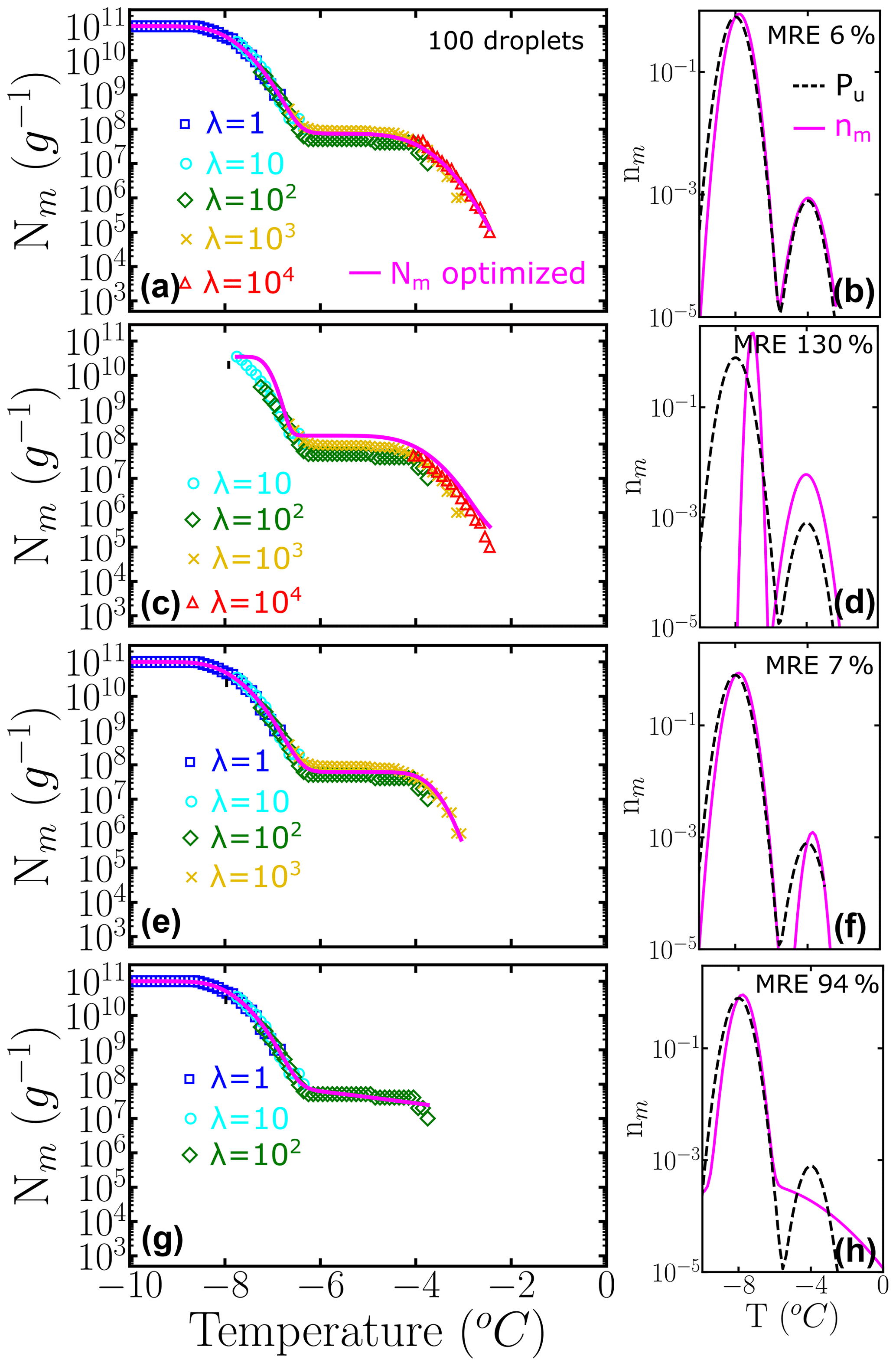
Figure 7Panels (a–d) represent the cumulative freezing spectra Nm(T) sampled from the same underlying distribution Pu(T). Colors represent the different number of INs per droplet: λ=1 (blue squares), λ=10 (cyan circles), λ=102 (green diamonds), λ=103 (yellow ×), and λ=104 (red triangles). The sampling was done using 100 droplets for each concentration. Panels (e–h) represent the differential freezing spectra nm(T) compared to the known underlying distribution Pu(T), shown by the magenta and dashed black lines, respectively. The mean relative error (MRE) was computed using Eq. (10) and the parameters of nm(T) and Pu(T) are shown in Table S2.

Figure 8Panels (a–c) represent the cumulative freezing spectra Nm(T) sampled from the same underlying distribution Pu(T). Colors represent the different number of INs per droplet: λ=1 (blue squares), λ=10 (cyan circles), λ=102 (green diamonds), λ=103 (yellow ×), and λ=104 (red triangles). The sampling was done using 25 droplets for each concentration. Panels (d–f) represent the differential freezing spectra nm(T) compared to the known underlying distribution Pu(T), shown by the magenta and dashed black lines, respectively. The mean relative error (MRE) was computed using Eq. (10). The parameters of nm(T) and Pu(T) are shown in Table S3.
3.2 Obtaining the differential freezing spectrum nm(T) from the experimental cumulative freezing spectrum Nm(T) of biological INs using the HUB-backward code
In this section we use the HUB-backward code to obtain the differential freezing spectrum nm(T) from the cumulative freezing spectra Nm(T) of the fungi Fusarium acuminatum strain 3–68 (Kunert et al., 2019), the bacterium P. syringae (Schwidetzky et al., 2021), and birch pollen (Dreischmeier, 2019). We select these systems because they are important biological INs and show increasing complexity in terms of the apparent number of underlying distributions that define their freezing spectra.
The experimental Nm(T) obtained for F. acuminatum (black squares in Fig. 9a) was obtained by sampling six 10-fold dilutions, each with 96 droplets (Kunert et al., 2019). Figure 9a shows the cumulative spectra optimized assuming one (green curve) and two (cyan curve) subpopulations; Fig. 9b shows the corresponding optimized differential freezing spectra. The with a single subpopulation that peaks at −5.9 ∘C is unable to represent the cumulative density of the most potent nuclei and misses the inflection at around −5.9 ∘C in the experimental data, resulting in a mean squared error MSE = 0.05. The with two subpopulations has a lower MSE = 0.003 and a better fit that suggests a population that peaks at −7.3 ∘C and another at −5.5 ∘C, in comparable amounts (Table 2). Most notably, the two subpopulations do not overlap in the differential freezing spectrum, supporting that they may indeed correspond to different physical entities. The improvement in the fit becomes apparent in the inset of Fig. 9a, which shows Nm(T) on a linear scale. The significant slope of Nm(T) even at the lowest temperatures indicates that the sampling of more diluted solutions is needed to capture the contribution of the less active INs. An attempt to represent F. acuminatum nucleation data with three different subpopulations resulted in two of them being almost identical. We conclude that adding a third subpopulation is unnecessary to reproduce the experimental cumulative freezing spectrum of F. acuminatum. We refer the reader to Schwidetzky et al. (2023) for an interpretation of the size of the ice-nucleating surface of F. acuminatum based on its differential spectrum and nucleation theory.

Figure 9Cumulative freezing spectra Nm(T) obtained from drop-freezing experiments for (a) F. acuminatum strain 3–68 (Kunert et al., 2019), (b) P. Syringae (Schwidetzky et al., 2021), and (c) birch pollen (Dreischmeier, 2019) (black circles). The solid green, long dashed cyan, and short dashed red lines represent computed with the optimized differential freezing spectra obtained with the HUB-backward code considering one, two, and three subpopulations, respectively. Panels (b), (d), and (e) show . The gray circles are experimental data points in the measurement of the birch pollen ice nucleation spectrum that were not considered in the optimization procedure. Insets in (a) and (c) show Nm(T) in normal scale.
Table 2Mean squared error (MSE) and parameters of the differential freezing spectra nm(T) obtained using the HUB-backward code and experimental data as input. The values shown here were calculated based on the average of n=3 independent runs. The error bars, shown in parentheses, were calculated by dividing the standard deviation of the values in these runs by 3.
Next, we apply the HUB-backward code to analyze the experimental freezing spectrum of Snomax®, i.e., inactivated P. syringae. The cumulative spectrum suggests the presence of two distinct subpopulations, usually called class A (at warmer temperatures) and class C (at colder ones). We first assume the differential freezing spectrum nm(T) of P. syringae is a combination of two Gaussian populations. The parameters of the optimized differential spectrum with two subpopulations are listed in Table 2, and the curve is shown in Fig. 9d with a cyan line. We use a logarithmic scale to represent this because the population corresponding to class A accounts for less than 0.1 % of the total (Table 2). While the fit with two subpopulations results in a good overall account of the target data, we note that there is some difference in the region between classes A and C (Fig. 9c). The fitting for P. syringae achieves an excellent agreement between optimized and target cumulative spectra (Fig. 9c), through the prediction of an additional peak located between classes A and C (the elusive class B), with a population comparable to class A (Table 2 and red curve in Fig. 9d). However, more measurements and analyses are needed to establish whether this “class B” peak at −5.2 ∘C is reproducible and truly distinct from the one of class A at −3.7 ∘C to warrant a physical interpretation. Overall, both the analyses with two and three subpopulations agree with previous ones (Govindarajan and Lindow, 1988; Warren, 1987) that concluded that over 99 % of the INs active in P. syringae bacteria in Snomax® belongs to class C. The analysis presented here for fungal and bacterial INs illustrates how HUB-backward can be used to reveal and characterize the underlying number of IN subpopulations of complex biological samples.
To further test the methodology, we model the cumulative freezing spectrum of birch pollen. Given that the original Nm(T) data for pollen in Fig. 3.1 of Dreischmeier (2019) consist of multiple independent curves, we took one of the many presented in this graph as the target (black curve in Fig. 9e) and present some of the additional data – not used in the optimization – with gray circles in Fig. 9e. Section S4 in the Supplement shows that the differential spectrum optimized from the whole data set and its sparse sampling are almost identical because HUB-forward interpolates and smooths the input data to produce an equispaced data set. The seems to contain three quite separated subpopulations, which is confirmed by the accuracy of the optimized cumulative spectrum in Fig. 9e. The parameters of the optimized differential freezing spectrum and the MSE are shown in Table 2. Our analysis indicates that the two subpopulations that nucleate ice above −16 ∘C constitute less than 0.01 % of the active nucleating sites in pollen (Fig. 9e), consistent with drop-freezing assays that only measured solutions with low concentrations of birch pollen and did not observe freezing at higher temperatures (Augustin et al., 2013; Pummer et al., 2012; Felgitsch et al., 2018), while the more extensive data of Dreischmeier (2019) reveal two more active subpopulations of INs.
To further illustrate the use of HUB-backward, Fig. 10 shows the effect of pH in the modes, spread, and weights of the subpopulations that contribute to the nucleation spectrum of P. syringae (Snomax®), using data from Lukas et al. (2020). Freezing in the temperature range of class A drops about 3 orders of magnitude when the pH is lowered from 6.2 to 4.4 (Fig. 10b). However, we note that the cumulative number of INs is preserved in the experimental cumulative freezing spectrum (Lukas et al., 2020), indicating that the change in pH did not impact the number of nucleants. Figure 10c and d demonstrate that the distributions associated with both subpopulations shift to lower temperatures when the pH decreases, and the range of freezing temperatures in class A becomes broader. An attempt to fit the cumulative spectra of Snomax at different pH values with the same subpopulations, allowing only for adjustment of their weights, resulted in a poor fit to the experimental Nm(T), supporting the conclusions of Lukas et al. (2020) of a central role of electrostatic interactions in the assembly of the bacterial ice-nucleating proteins and their ability to bind to ice. This analysis exemplifies how HUB-backward can be applied to quantify the dependence of IN on environmental variables.
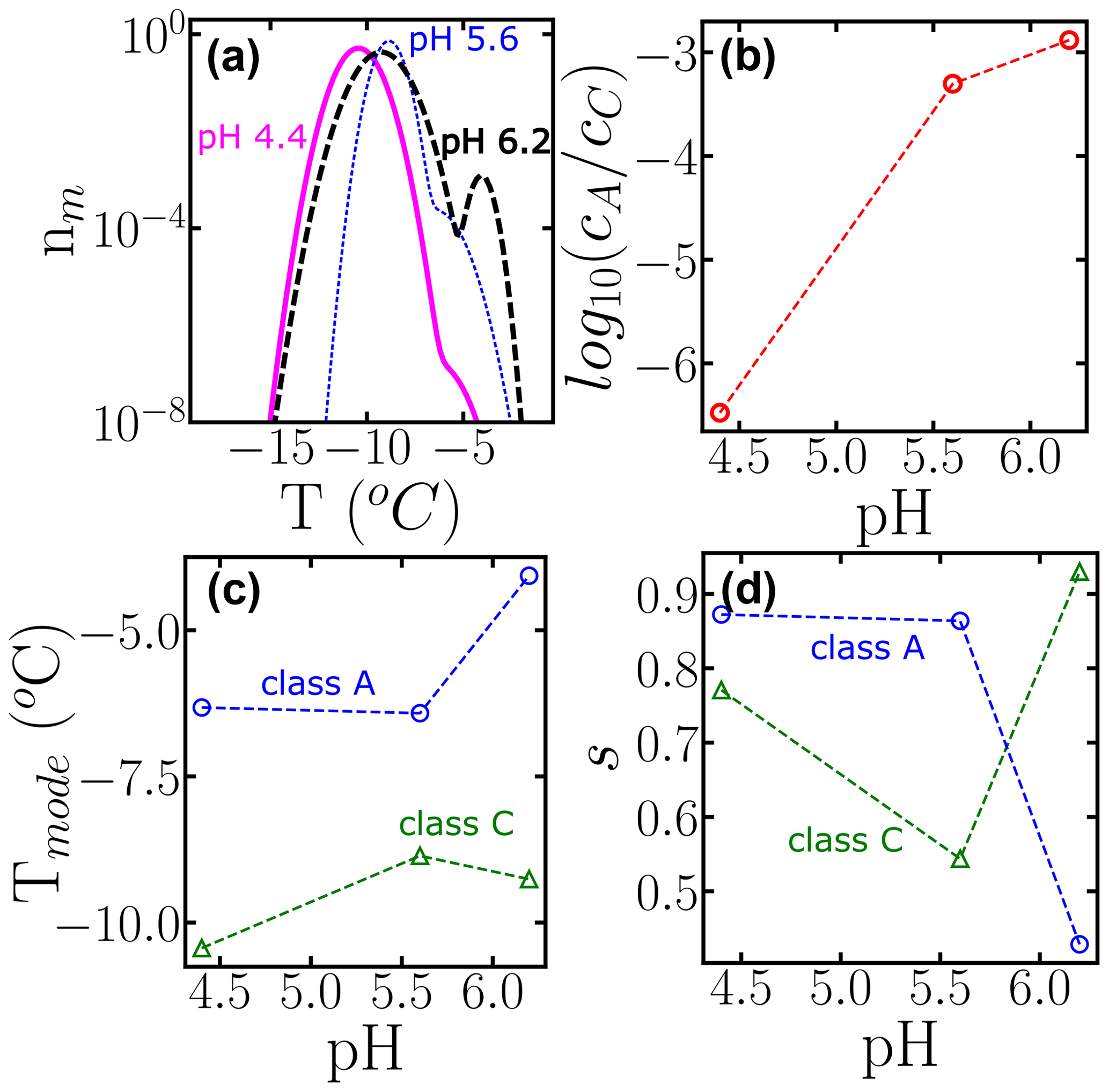
Figure 10Effect of changing the pH on the subpopulations of P. Syringae (Lukas et al., 2020). (a) Differential freezing spectra nm(T) obtained using the HUB-backward code. Colors represent the different pH values: 6.5 (long dashed black line), 5.6 (short dotted blue line), and 4.4 (solid magenta line). (b) Ratio between the weights, (c) the modes, and (d) the spreads of each subpopulation as a function of pH. The fitting of Nm(T) and the parameters of nm(T) are shown in Fig. S1 and Table S4.
3.3 Obtaining the differential freezing spectrum nm(T) from the experimental fraction of ice fice(T) of insoluble ice nucleators using the HUB-backward code
Section 3.1 and 3.2 discuss how to obtain the differential spectrum from a target cumulative one. However, there are many cases where the results are presented as a fraction of frozen droplets as a function of temperature, fice(T). In these cases, the HUB-backward code can be used to obtain the optimized differential freezing spectrum directly from . Section S5 illustrates this approach for the analysis of droplet freezing data for a sample of lignin (Bogler and Borduas-Dedekind, 2020) in which the INs participate in aggregation equilibria. Here, we exemplify the optimization of the differential spectrum of cholesterol from experimental freezing data obtained at two cooling rates with droplets sampled from a single dilution.
In the analysis of drop-freezing experiments, it is assumed that each IN has a singular freezing temperature, independent of the cooling rate. However, ice nucleation is a stochastic process, and the underlying distribution of freezing temperatures Pu(T) strictly depends on both temperature and cooling rate, as slower rates give more time for the system to cross the nucleation barrier at warmer temperatures.
The triangles and squares in Fig. 11a display the experimental fice(T) obtained by sampling the freezing of hundreds of 120 µL droplets pipetted from a suspension of cholesterol monohydrate crystals in contact with Teflon cooled at 0.18 K min−1 (triangles) and 0.06 K min−1 (squares) (Zhang and Maeda, 2022). Our analysis of the freezing data of cholesterol monohydrate shows that even a 3-fold change in the cooling rate can have a significant effect on the differential spectrum (Fig. 11b).

Figure 11Use of the HUB-backward code to estimate the optimized differential freezing spectra based on the fraction of frozen droplets of cholesterol (Zhang and Maeda, 2022) at different cooling rates. Black circles and squares are experimental data, and dashed cyan and solid red lines are the optimized differential spectra given by the HUB-backward code. The parameters of nm(T) are shown in Table S5.
As expected, the modes of the three populations move towards warmer temperatures upon decreasing the cooling rate. We note, however, that the shift in the peaks is not uniform; the middle one seems to be more sensitive to the cooling rate. Different sensitivity of the freezing rate of subpopulations has also been reported in simulations of nucleation data of minerals using the stochastic and modified singular frameworks (Herbert et al., 2014; Murray et al., 2011). The modified singular model proposes an empirical correction to the relation between fice(T) and Nm(T) to account for the effect of the cooling rate on the shift in these quantities (Vali, 1994). That analysis could be extended to the analysis of the subpopulations of INs obtained with HUB-backward. Moreover, it would be interesting in future studies to use the rate dependence of the mode of the subpopulations to extract the steepness of the nucleation barrier with temperature using nucleation theory (Budke and Koop, 2015) and to investigate the relationship between the cooling rate dependence of the differential spectrum obtained in the singular approximation with the interpretation of the same data modeled with the stochastic framework, such as in Wright et al. (2013) and Herbert et al. (2014).
In this study, we present the HUB method and associated Python codes that model (HUB-forward code) and interpret (HUB-backward code) the results of droplet freezing experiments under the assumptions that each ice-nucleating site in the sample has a characteristic nucleation temperature that is time-independent. The use of the singular approximation is the same as that used by Vali (1971, 2014, 2019) in his derivation of the ice nucleation spectra from data of fraction of frozen droplets. Different to previous implementations of the singular model, HUB accounts for the distribution of the number of INs in droplets at a given concentration and uses extreme value statistics to represent the effect of dilutions in the frozen fraction and freezing spectra. Our method and codes allow users to obtain an analytical differential freezing spectrum nm(T) from the experimental distribution of freezing temperatures, and vice versa. The differential freezing spectrum nm(T) is an approximant to the underlying distribution of ice-nucleating temperatures Pu(T), which provides a hub to connect the experimental freezing temperatures with interpretative physical analyses using kinetic models or nucleation theory that can be used to elucidate the mechanisms of nucleation and origins of these distributions.
HUB-forward predicts the cumulative ice nucleation spectrum Nm(T) and fractions of frozen droplets fice(T) from a known (or assumed) underlying distribution Pu(T) of nucleation temperatures for the INs in the sample. The HUB-forward code can be used to investigate the effect of the number of droplets and dilutions on the temperature range of the cumulative freezing spectrum Nm(T). Our analysis shows that the differential freezing spectrum nm(T) is identical to the underlying distribution of heterogeneous ice nucleation temperatures Pu(T) only when sampling is complete. Measuring fewer droplets or fewer dilutions can result in a biased representation of the differential and cumulative spectra. HUB-forward predicts fice(T) and Nm(T) from a proposed distribution of IN temperatures, allowing its users to test hypotheses regarding the role of subpopulations of nuclei in the freezing spectra and providing a guide for a more efficient collection of freezing data.
HUB-backward uses a non-linear optimization method to find the differential freezing spectrum nm(T) that best represents the experimental target cumulative freezing spectrum Nm(T) or fraction of frozen droplets fice(T) in the experiments. The analytical form of the differential freezing spectrum nm(T) obtained from HUB-backward offers an interpretable physical basis. The interpretability of the results in terms of subpopulations provides an advantage over polynomial fitting and differentiation of Nm(T). Indeed, we show that the HUB-backward code can be used to reveal and characterize the underlying number of IN subpopulations of complex biological samples (Snomax®, fungi Fusarium acuminatum, and birch pollen) and quantify the dependence of their subpopulations on environmental variables. Interestingly, our analysis evinces subpopulations that are not obvious to the eye and have not previously been identified in these samples. The robustness of the signals that correspond to these populations and their physical nature require further investigation.
We illustrate the use of HUB-backward to obtain the differential freezing spectrum nm(T) from the fraction of frozen droplets fice(T) collected at a single concentration. We apply that analysis to demonstrate that nm(T) depends on the cooling rate. The shift in the peaks of the subpopulations to higher temperatures upon decreasing the cooling rate is not unexpected, as longer waiting times allow for the surmounting of the same nucleation barrier at warmer temperatures. By providing the temperature dependence of the mode, spread, and weight of the subpopulation peaks, HUB-backward can be combined with nucleation theory and other theoretical analyses to extract the steepness, and maybe even the distribution, of nucleation barriers that control the freezing process.
All codes, a user manual, and input files used in this project can be accessed at https://github.com/Molinero-Group/underlying-distribution (last access: 5 May 2023) and https://doi.org/10.5281/zenodo.7901549 (de Almeida Ribeiro et al., 2023).
All data used in this project can be accessed upon request to the authors.
The supplement related to this article is available online at: https://doi.org/10.5194/acp-23-5623-2023-supplement.
VM, IdAR, and KM designed the project. IdAR developed the model code and performed the simulations. IdAR and VM prepared the manuscript with contributions from KM.
The contact author has declared that none of the authors has any competing interests.
Publisher's note: Copernicus Publications remains neutral with regard to jurisdictional claims in published maps and institutional affiliations.
Ingrid de Almeida Ribeiro and Valeria Molinero gratefully acknowledge support by AFOSR through MURI award no. FA9550-20-1-0351. Konrad Meister acknowledges support by the National Science Foundation under grant no. NSF 2116528 and from the Institutional Development Awards (IDeA) from the National Institute of General Medical Sciences of the National Institutes of Health under grant nos. P20GM103408 and P20GM109095.
This research has been supported by the Air Force Office of Scientific Research (grant no. FA9550-20-1-0351), the National Institutes of Health (grant nos. P20GM103408 and P20GM109095), and the National Science Foundation (grant no. 2116528).
This paper was edited by Daniel Knopf and reviewed by Nadine Borduas-Dedekind and one anonymous referee.
Alpert, P. A. and Knopf, D. A.: Analysis of isothermal and cooling-rate-dependent immersion freezing by a unifying stochastic ice nucleation model, Atmos. Chem. Phys., 16, 2083–2107, https://doi.org/10.5194/acp-16-2083-2016, 2016.
Augustin, S., Wex, H., Niedermeier, D., Pummer, B., Grothe, H., Hartmann, S., Tomsche, L., Clauss, T., Voigtländer, J., Ignatius, K., and Stratmann, F.: Immersion freezing of birch pollen washing water, Atmos. Chem. Phys., 13, 10989–11003, https://doi.org/10.5194/acp-13-10989-2013, 2013.
Bigg, E.: The formation of atmospheric ice crystals by the freezing of droplets, Q. J. Roy. Meteor. Soc., 79, 510–519, 1953.
Bogler, S. and Borduas-Dedekind, N.: Lignin's ability to nucleate ice via immersion freezing and its stability towards physicochemical treatments and atmospheric processing, Atmos. Chem. Phys., 20, 14509–14522, https://doi.org/10.5194/acp-20-14509-2020, 2020.
Broadley, S. L., Murray, B. J., Herbert, R. J., Atkinson, J. D., Dobbie, S., Malkin, T. L., Condliffe, E., and Neve, L.: Immersion mode heterogeneous ice nucleation by an illite rich powder representative of atmospheric mineral dust, Atmos. Chem. Phys., 12, 287–307, https://doi.org/10.5194/acp-12-287-2012, 2012.
Budke, C. and Koop, T.: BINARY: an optical freezing array for assessing temperature and time dependence of heterogeneous ice nucleation, Atmos. Meas. Tech., 8, 689–703, https://doi.org/10.5194/amt-8-689-2015, 2015.
Carte, A.: The freezing of water droplets, P. Phys. Soc. B, 69, 1028–1037, 1956.
Castillo, E., Hadi, A. S., Balakrishnan, N., and Sarabia, J. M.: Extreme value and related models in engineering and science applications, John Wiley & Sons, New York, 179, ISBN 9780471671725, 2005.
Creamean, J. M., Mignani, C., Bukowiecki, N., and Conen, F.: Using freezing spectra characteristics to identify ice-nucleating particle populations during the winter in the Alps, Atmos. Chem. Phys., 19, 8123–8140, https://doi.org/10.5194/acp-19-8123-2019, 2019.
David, H. A. and Nagaraja, H. N.: Order Statistics. Wiley, ISBN 9780471654018, 2004.
de Almeida Ribeiro, I., Meister, K., and Molinero, V.: Codes and data for “HUB: a method to model and extract the distribution of ice nucleation temperatures from drop-freezing experiments” (v1.0), Zenodo [code and data set], https://doi.org/10.5281/zenodo.7901549, 2023.
de Haan, L. and Ferreira, A.: Extreme Value Theory: An Introduction, Springer New York, ISBN 9780387344713, 2007.
DeMott, P. J., Cziczo, D. J., Prenni, A. J., Murphy, D. M., Kreidenweis, S. M., Thomson, D. S., Borys, R., and Rogers, D. C.: Measurements of the concentration and composition of nuclei for cirrus formation, P. Natl. Acad. Sci. USA, 100, 14655–14660, https://doi.org/10.1073/pnas.2532677100, 2003.
DeMott, P. J., Hill, T. C. J., McCluskey, C. S., Prather, K. A., Collins, D. B., Sullivan, R. C., Ruppel, M. J., Mason, R. H., Irish, V. E., Lee, T., Hwang, C. Y., Rhee, T. S., Snider, J. R., McMeeking, G. R., Dhaniyala, S., Lewis, E. R., Wentzell, J. J. B., Abbatt, J., Lee, C., Sultana, C. M., Ault, A. P., Axson, J. L., Martinez, M. D., Venero, I., Santos-Figueroa, G., Stokes, M. D., Deane, G. B., Mayol-Bracero, O. L., Grassian, V. H., Bertram, T. H., Bertram, A. K., Moffett, B. F., and Franc, G. D.: Sea spray aerosol as a unique source of ice nucleating particles, P. Natl. Acad. Sci. USA, 113, 5797–5803, https://doi.org/10.1073/pnas.1514034112, 2016.
Dreischmeier, K.: Heterogene Eisnukleations- und Antigefriereigenschaften von Biomolekülen, Bielefeld University, https://doi.org/10.4119/unibi/2907691, 2019.
Fahy, W. D., Maters, E. C., Giese Miranda, R., Adams, M. P., Jahn, L. G., Sullivan, R. C., and Murray, B. J.: Volcanic ash ice nucleation activity is variably reduced by aging in water and sulfuric acid: the effects of leaching, dissolution, and precipitation, Environ. Sci.-Atmos., 2, 85–99, https://doi.org/10.1039/D1EA00071C, 2022a.
Fahy, W. D., Shalizi, C. R., and Sullivan, R. C.: A universally applicable method of calculating confidence bands for ice nucleation spectra derived from droplet freezing experiments, Atmos. Meas. Tech., 15, 6819–6836, https://doi.org/10.5194/amt-15-6819-2022, 2022b.
Felgitsch, L., Baloh, P., Burkart, J., Mayr, M., Momken, M. E., Seifried, T. M., Winkler, P., Schmale III, D. G., and Grothe, H.: Birch leaves and branches as a source of ice-nucleating macromolecules, Atmos. Chem. Phys., 18, 16063–16079, https://doi.org/10.5194/acp-18-16063-2018, 2018.
Fletcher, N. H.: Active sites and ice crystal nucleation, J. Atmos. Sci., 26, 1266–1271, 1969.
Froyd, K. D., Yu, P., Schill, G. P., Brock, C. A., Kupc, A., Williamson, C. J., Jensen, E. J., Ray, E., Rosenlof, K. H., Bian, H., Darmenov, A. S., Colarco, P. R., Diskin, G. S., Bui, T., and Murphy, D. M.: Dominant role of mineral dust in cirrus cloud formation revealed by global-scale measurements, Nat. Geosci., 15, 177–183, https://doi.org/10.1038/s41561-022-00901-w, 2022.
Gettelman, A., Liu, X., Barahona, D., Lohmann, U., and Chen, C.: Climate impacts of ice nucleation, J. Geophys. Res.-Atmos., 117, D20201, https://doi.org/10.1029/2012JD017950, 2012.
Govindarajan, A. G. and Lindow, S. E.: Size of bacterial ice-nucleation sites measured in situ by radiation inactivation analysis, P. Natl. Acad. Sci. USA, 85, 1334–1338, https://doi.org/10.1073/pnas.85.5.1334, 1988.
Gumbel, E. J. Statistics of Extremes, Dover Publications, ISBN 9780486154480, 2012.
Harrison, A. D., Whale, T. F., Carpenter, M. A., Holden, M. A., Neve, L., O'Sullivan, D., Vergara Temprado, J., and Murray, B. J.: Not all feldspars are equal: a survey of ice nucleating properties across the feldspar group of minerals, Atmos. Chem. Phys., 16, 10927–10940, https://doi.org/10.5194/acp-16-10927-2016, 2016.
Hartmann, S., Ling, M., Dreyer, L. S. A., Zipori, A., Finster, K., Grawe, S., Jensen, L. Z., Borck, S., Reicher, N., Drace, T., Niedermeier, D., Jones, N. C., Hoffmann, S. V., Wex, H., Rudich, Y., Boesen, T., and Šantl-Temkiv, T.: Structure and Protein-Protein Interactions of Ice Nucleation Proteins Drive Their Activity, bioRxiv, 2022.2001.2021.477219, https://doi.org/10.1101/2022.01.21.477219, 2022.
Herbert, R. J., Murray, B. J., Whale, T. F., Dobbie, S. J., and Atkinson, J. D.: Representing time-dependent freezing behaviour in immersion mode ice nucleation, Atmos. Chem. Phys., 14, 8501–8520, https://doi.org/10.5194/acp-14-8501-2014, 2014.
Knopf, D. A., Alpert, P. A., Zipori, A., Reicher, N., and Rudich, Y.: Stochastic nucleation processes and substrate abundance explain time-dependent freezing in supercooled droplets, NPJ Climate and Atmospheric Science, 3, 2, https://doi.org/10.1038/s41612-020-0106-4, 2020.
Kunert, A. T., Lamneck, M., Helleis, F., Pöschl, U., Pöhlker, M. L., and Fröhlich-Nowoisky, J.: Twin-plate Ice Nucleation Assay (TINA) with infrared detection for high-throughput droplet freezing experiments with biological ice nuclei in laboratory and field samples, Atmos. Meas. Tech., 11, 6327–6337, https://doi.org/10.5194/amt-11-6327-2018, 2018.
Kunert, A. T., Pöhlker, M. L., Tang, K., Krevert, C. S., Wieder, C., Speth, K. R., Hanson, L. E., Morris, C. E., Schmale III, D. G., Pöschl, U., and Fröhlich-Nowoisky, J.: Macromolecular fungal ice nuclei in Fusarium: effects of physical and chemical processing, Biogeosciences, 16, 4647–4659, https://doi.org/10.5194/bg-16-4647-2019, 2019.
Levine, J.: Statistical explanation of spontaneous freezing of water droplets, NACA Tech. Note, 2234, 1950.
Lukas, M., Schwidetzky, R., Kunert, A. T., Pöschl, U., Fröhlich-Nowoisky, J., Bonn, M., and Meister, K.: Electrostatic Interactions Control the Functionality of Bacterial Ice Nucleators, J. Am. Chem. Soc., 142, 6842–6846, https://doi.org/10.1021/jacs.9b13069, 2020.
Lukas, M., Schwidetzky, R., Eufemio, R. J., Bonn, M., and Meister, K.: Toward Understanding Bacterial Ice Nucleation, J. Phys. Chem. B, 126, 1861–1867, https://doi.org/10.1021/acs.jpcb.1c09342, 2022.
Marcolli, C., Gedamke, S., Peter, T., and Zobrist, B.: Efficiency of immersion mode ice nucleation on surrogates of mineral dust, Atmos. Chem. Phys., 7, 5081–5091, https://doi.org/10.5194/acp-7-5081-2007, 2007.
Miller, A. J., Brennan, K. P., Mignani, C., Wieder, J., David, R. O., and Borduas-Dedekind, N.: Development of the drop Freezing Ice Nuclei Counter (FINC), intercomparison of droplet freezing techniques, and use of soluble lignin as an atmospheric ice nucleation standard, Atmos. Meas. Tech., 14, 3131–3151, https://doi.org/10.5194/amt-14-3131-2021, 2021.
Mülmenstädt, J., Sourdeval, O., Delanoë, J., and Quaas, J.: Frequency of occurrence of rain from liquid-, mixed-, and ice-phase clouds derived from A-Train satellite retrievals, Geophys. Res. Lett., 42, 6502–6509, https://doi.org/10.1002/2015GL064604, 2015.
Murray, B. J., Broadley, S. L., Wilson, T. W., Atkinson, J. D., and Wills, R. H.: Heterogeneous freezing of water droplets containing kaolinite particles, Atmos. Chem. Phys., 11, 4191–4207, https://doi.org/10.5194/acp-11-4191-2011, 2011.
Murray, B. J., O'Sullivan, D., Atkinson, J. D., and Webb, M. E.: Ice nucleation by particles immersed in supercooled cloud droplets, Chem. Soc. Rev., 41, 6519–6554, https://doi.org/10.1039/C2CS35200A, 2012.
Niedermeier, D., Shaw, R. A., Hartmann, S., Wex, H., Clauss, T., Voigtländer, J., and Stratmann, F.: Heterogeneous ice nucleation: exploring the transition from stochastic to singular freezing behavior, Atmos. Chem. Phys., 11, 8767–8775, https://doi.org/10.5194/acp-11-8767-2011, 2011.
Pummer, B. G., Bauer, H., Bernardi, J., Bleicher, S., and Grothe, H.: Suspendable macromolecules are responsible for ice nucleation activity of birch and conifer pollen, Atmos. Chem. Phys., 12, 2541–2550, https://doi.org/10.5194/acp-12-2541-2012, 2012.
Reicher, N., Segev, L., and Rudich, Y.: The WeIzmann Supercooled Droplets Observation on a Microarray (WISDOM) and application for ambient dust, Atmos. Meas. Tech., 11, 233–248, https://doi.org/10.5194/amt-11-233-2018, 2018.
Satopaa, V., Albrecht, J., Irwin, D., and Raghavan, B.: Finding a “Kneedle” in a Haystack: Detecting Knee Points in System Behavior, 2011 31st International Conference on Distributed Computing Systems Workshops, 20–24 June 2011, 166–171, https://doi.org/10.1109/ICDCSW.2011.20, 2011.
Schwidetzky, R., Sudera, P., Backes, A. T., Pöschl, U., Bonn, M., Fröhlich-Nowoisky, J., and Meister, K.: Membranes Are Decisive for Maximum Freezing Efficiency of Bacterial Ice Nucleators, J. Phys. Chem. Lett., 12, 10783–10787, https://doi.org/10.1021/acs.jpclett.1c03118, 2021.
Schwidetzky, R., de Almeida Ribeiro, I., Bothen, N., Backes, A., DeVries, A. L., Bonn, M., Frhlich-Nowoisky, J., Molinero, V., and Meister, K.: E Pluribus Unum: Functional Aggregation Enables Biological Ice Nucleation, ChemRxiv, Cambridge Open Engage, Cambridge, https://doi.org/10.26434/chemrxiv-2023-63qfl, 2023.
Sear, R. P.: Generalisation of Levine's prediction for the distribution of freezing temperatures of droplets: a general singular model for ice nucleation, Atmos. Chem. Phys., 13, 7215–7223, https://doi.org/10.5194/acp-13-7215-2013, 2013.
Steinke, I., Hiranuma, N., Funk, R., Höhler, K., Tüllmann, N., Umo, N. S., Weidler, P. G., Möhler, O., and Leisner, T.: Complex plant-derived organic aerosol as ice-nucleating particles – more than the sums of their parts?, Atmos. Chem. Phys., 20, 11387–11397, https://doi.org/10.5194/acp-20-11387-2020, 2020.
Stratmann, F., Kiselev, A., Wurzler, S., Wendisch, M., Heintzenberg, J., Charlson, R. J., Diehl, K., Wex, H., and Schmidt, S.: Laboratory Studies and Numerical Simulations of Cloud Droplet Formation under Realistic Supersaturation Conditions, J. Atmos. Ocean. Tech., 21, 876–887, https://doi.org/10.1175/1520-0426(2004)021<0876:Lsanso>2.0.Co;2, 2004.
Turner, M. A., Arellano, F., and Kozloff, L. M.: Three separate classes of bacterial ice nucleation structures, J. Bacteriol., 172, 2521–2526, https://doi.org/10.1128/jb.172.5.2521-2526.1990, 1990.
Vali, G.: Quantitative Evaluation of Experimental Results an the Heterogeneous Freezing Nucleation of Supercooled Liquids, J. Atmos. Sci., 28, 402–409, https://doi.org/10.1175/1520-0469(1971)028<0402:Qeoera>2.0.Co;2, 1971.
Vali, G.: Freezing rate due to heterogeneous nucleation, J. Atmos. Sci., 51, 1843–1856, 1994.
Vali, G.: Interpretation of freezing nucleation experiments: singular and stochastic; sites and surfaces, Atmos. Chem. Phys., 14, 5271–5294, https://doi.org/10.5194/acp-14-5271-2014, 2014.
Vali, G.: Revisiting the differential freezing nucleus spectra derived from drop-freezing experiments: methods of calculation, applications, and confidence limits, Atmos. Meas. Tech., 12, 1219–1231, https://doi.org/10.5194/amt-12-1219-2019, 2019.
Vali, G. and Stansbury, E. J.: TIME-DEPENDENT CHARACTERISTICS OF THE HETEROGENEOUS NUCLEATION OF ICE, Can. J. Phys., 44, 477–502, https://doi.org/10.1139/p66-044, 1966.
Virtanen, P., Gommers, R., Oliphant, T. E., Haberland, M., Reddy, T., Cournapeau, D., Burovski, E., Peterson, P., Weckesser, W., Bright, J., van der Walt, S. J., Brett, M., Wilson, J., Millman, K. J., Mayorov, N., Nelson, A. R. J., Jones, E., Kern, R., Larson, E., Carey, C. J., Polat, Ý., Feng, Y., Moore, E. W., VanderPlas, J., Laxalde, D., Perktold, J., Cimrman, R., Henriksen, I., Quintero, E. A., Harris, C. R., Archibald, A. M., Ribeiro, A. H., Pedregosa, F., van Mulbregt, P., Vijaykumar, A., Bardelli, A. P., Rothberg, A., Hilboll, A., Kloeckner, A., Scopatz, A., Lee, A., Rokem, A., Woods, C. N., Fulton, C., Masson, C., Häggström, C., Fitzgerald, C., Nicholson, D. A., Hagen, D. R., Pasechnik, D. V., Olivetti, E., Martin, E., Wieser, E., Silva, F., Lenders, F., Wilhelm, F., Young, G., Price, G. A., Ingold, G.-L., Allen, G. E., Lee, G. R., Audren, H., Probst, I., Dietrich, J. P., Silterra, J., Webber, J. T., Slaviè, J., Nothman, J., Buchner, J., Kulick, J., Schönberger, J. L., de Miranda Cardoso, J. V., Reimer, J., Harrington, J., Rodríguez, J. L. C., Nunez-Iglesias, J., Kuczynski, J., Tritz, K., Thoma, M., Newville, M., Kümmerer, M., Bolingbroke, M., Tartre, M., Pak, M., Smith, N. J., Nowaczyk, N., Shebanov, N., Pavlyk, O., Brodtkorb, P. A., Lee, P., McGibbon, R. T., Feldbauer, R., Lewis, S., Tygier, S., Sievert, S., Vigna, S., Peterson, S., More, S., Pudlik, T., Oshima, T., Pingel, T. J., Robitaille, T. P., Spura, T., Jones, T. R., Cera, T., Leslie, T., Zito, T., Krauss, T., Upadhyay, U., Halchenko, Y. O., Vázquez-Baeza, Y., and SciPy, C.: SciPy 1.0: fundamental algorithms for scientific computing in Python, Nature Methods, 17, 261–272, https://doi.org/10.1038/s41592-019-0686-2, 2020.
Warren, G. J.: Bacterial Ice Nucleation: Molecular Biology and Applications, Biotechnol. Genet. Eng., 5, 107–136, https://doi.org/10.1080/02648725.1987.10647836, 1987.
Wright, T. P. and Petters, M. D.: The role of time in heterogeneous freezing nucleation, J. Geophys. Res.-Atmos., 118, 3731–3743, https://doi.org/10.1002/jgrd.50365, 2013.
Wright, T. P., Petters, M. D., Hader, J. D., Morton, T., and Holder, A. L.: Minimal cooling rate dependence of ice nuclei activity in the immersion mode, J. Geophys. Res.-Atmos., 118, 10535–10543, https://doi.org/10.1002/jgrd.50810, 2013.
Zhang, X. and Maeda, N.: Nucleation curves of ice in the presence of nucleation promoters, Chem. Eng. Sci., 262, 118017, https://doi.org/10.1016/j.ces.2022.118017, 2022.
Zobrist, B., Koop, T., Luo, B., Marcolli, C., and Peter, T.: Heterogeneous ice nucleation rate coefficient of water droplets coated by a nonadecanol monolayer, J. Phys. Chem. C, 111, 2149–2155, 2007.
- Abstract
- Introduction
- Numerical modeling of drop-freezing experiments
- Using the HUB code to optimize and analyze drop-freezing experiments
- Conclusions
- Code availability
- Data availability
- Author contributions
- Competing interests
- Disclaimer
- Acknowledgements
- Financial support
- Review statement
- References
- Supplement