The future ozone trends in changing climate simulated with SOCOLv4

This study evaluates the future evolution of atmospheric ozone simulated with the Earth system model (ESM) SOCOLv4. Simulations have been performed based on two potential shared socioeconomic pathways (SSPs): the middle-of-the-road (SSP2-4.5) and fossil-fueled (SSP5-8.5) scenarios. The future changes in ozone, as well as in chemical drivers (NO_x and CO) and temperature, were estimated between 2015 and 2099 and for several intermediate subperiods (i.e., 2015–2039, 2040–2069, and 2070–2099) via dynamic linear modeling. In both scenarios, the model projects a decline in tropospheric ozone in the future that starts in the 2030s in SSP2-4.5 and after the 2060s in SSP5-8.5 due to a decrease in concentrations of NO_x and CO. The results also suggest a very likely ozone increase in the mesosphere and the upper and middle stratosphere, as well as in the lower stratosphere at high latitudes. Under SSP5-8.5, the ozone increase in the stratosphere is higher because of stronger cooling (>1 K per decade) induced by greenhouse gases (GHGs), which slows the catalytic ozone destruction cycles. In contrast, in the tropical lower stratosphere, ozone concentrations decrease in both experiments and increase over the middle and high latitudes of both hemispheres due to the speeding up of the Brewer–Dobson circulation, which is stronger in SSP5-8.5. No evidence was found of a decline in ozone levels in the lower stratosphere at mid-latitudes. In both future scenarios, the total column ozone is expected to be distinctly higher than present in middle to high latitudes and might be lower in the tropics, which causes a decrease in the mid-latitudes and an increase in the tropics in the surface level of ultraviolet radiation. The results of SOCOLv4 suggest that the stratospheric-ozone evolution throughout the 21st century is strongly governed not only by a decline in halogen concentration but also by future GHG forcing. In addition, the tropospheric-ozone column changes, which are mainly due to the changes in anthropogenic emissions of ozone precursors, also have a strong impact on the total column. Therefore, even though the anthropogenic halogen-loading problem has been brought under control to date, the sign of future ozone column changes, globally and regionally, is still unclear and largely depends on diverse future human activities. The results of this work are, thus, relevant for developing future strategies for socioeconomic pathways.

1 Introduction

The stratospheric-ozone layer plays an essential role in the Earth’s atmosphere. It shields the ecosystem from dangerous ultraviolet radiation, shapes the vertical temperature profiles, and thus affects the general circulation of the atmosphere. The tropospheric ozone is one of the most potent greenhouse gases (GHGs; e.g., IPCC, 2021), contributing to the rise in near-surface temperature, as well as a toxic air pollutant that is harmful to human health and vegetation. Thus, ozone contributes not only to climate change but also to human, agriculture, and ecosystem development (e.g., Barnes et al., 2019).

A serious challenge for humanity is the consequences of stratospheric-ozone depletion caused by man-made halogenated ozone-depleting substances (hODSs). This prompted nations to ratify the Montreal Protocol in 1987, an international treaty to phase out hODSs. The Montreal Protocol and its Amendments and Adjustments (MPA) allows the ozone layer to recover from the hODS effect. Various studies show that the total ozone column decrease has been reversed at most latitudes, which is attributed to the decline in hODS concentrations, highlighting the success of the MPA in protecting the ozone layer (Newchurch et al., 2003; Solomon et al., 2016; WMO, 2018; Pazmiño et al., 2018; Kuttippurath et al., 2018; McKenzie et al., 2019). Different projections of the future ozone layer evolution during the 21st century suggest that the decrease in hODSs facilitates ozone recovery in the stratosphere (Banerjee et al., 2016). Ozone abundances are expected to return to the pre-1960 level in most atmospheric layers by the middle to late century, except in the lower stratosphere (Eyring et al., 2007; Austin et al., 2010; Dhomse et al., 2018; Keeble et al., 2021). Thus, it is believed that declining hODSs will gradually lose their leading role in determining the evolution of the ozone layer throughout the 21st century (Newman, 2018).

Studies claim that GHGs, such as carbon dioxide (CO₂), methane (CH₄), and nitrous oxide (N₂O), will largely control ozone changes in the 21st century (Morgenstern et al., 2018; Dhomse et al., 2018; Keeble et al., 2021). CO₂ facilitates the stratospheric-ozone enhancement due to direct radiative cooling of the stratosphere, slowing down the gas-phase ozone destruction rate (Randeniya et al., 2002; Stolarski et al., 2015). Therefore, for some parts of the stratosphere, even a super-recovery (i.e., ozone levels well above the pre-1980s level) is expected (Eyring et al., 2007; Meul et al., 2016).

Whilst N₂O is mainly inert in the troposphere, the growth of its concentration will hamper the increase of the stratospheric ozone in the future (Ravishankara et al., 2009; Chipperfield, 2009; Revell et al., 2012, 2015a; Stolarski et al., 2015) due to the increased production of nitrogen oxides (NO_x = NO + NO₂), which catalytically destroy ozone (Crutzen, 1970). Yet, the GHG-related cooling of the stratosphere may reduce the efficiency of catalytic cycles involving NO_x. This is due to the fact that more NO_x is converted to inactive N₂; i.e., the N₂O contribution to ozone destruction can be somewhat lowered (Revell et al., 2015a).

CH₄ plays an ambivalent role in ozone change, as it may have both negative and positive effects on ozone. The negative effect of increased CH₄ on stratospheric ozone is that it increases the efficiency of the hydroxyl oxide (HO_x) catalytic cycle of ozone destruction, since CH₄ is the main source of H₂O in the middle atmosphere (Bates and Nicolet, 1950). However, it should be noted that additional HO_x and NO_x radicals would also partly compensate for the negative effects of each other in the stratosphere through the production of the reservoir species HNO₃ (OH + NO₂ + M → HNO₃ + M). CH₄ also has a positive effect on ozone, as it causes an additional chlorine deactivation (CH₄ + Cl → CH₃ + HCl) throughout the stratosphere (Hitchman and Brasseur, 1988) and promotes an increase in tropospheric ozone by being a source of CO (Brasseur and Solomon, 2005; Morgenstern et al., 2013), which is a precursor for ozone formation in the lower atmosphere.

The future evolution of tropospheric ozone will be strongly driven by the changes in CO and NO_x, leading to large differences in projections of tropospheric ozone for distinct climate scenarios (Revell et al., 2015b; Archibald et al., 2020). In addition, the projections indicate that the future ozone changes in the troposphere are even more non-linear than in the stratosphere (Revell et al., 2015b).

Most chemistry–climate models (CCMs) project that the ozone layer will continue to thin in the tropical lower stratosphere throughout the 21st century (Zubov et al., 2013; Banerjee et al., 2016; Dhomse et al., 2018; Keeble et al., 2021). The speed of this thinning depends on the climate scenario for GHGs (Morgenstern et al., 2018; Dhomse et al., 2018; Keeble et al., 2021; Shang et al., 2021). GHG-induced temperature changes in the lower atmosphere strengthen the meridional transport via the shallow branch of the Brewer–Dobson circulation (BDC) due to an increase in the temperature gradient between tropical and mid-latitudes. This raises the tropopause, alters the wave propagation and dissipation, and extends the subtropical transport barriers upward (Zubov et al., 2013; Butchart, 2014; Chiodo et al., 2018; Abalos and de la Cámara, 2020). The faster atmospheric upwelling decreases the ozone production in the ascending air parcel (Avallone and Prather, 1996). The intensified transport also increases the stratosphere–troposphere exchange, with more ozone-poor tropospheric air being transported to the lower stratosphere (WMO, 2018). Models also exhibit significant differences in the magnitude of the simulated GHG-induced acceleration of the BDC (Morgenstern et al., 2018).

Projections of the ozone layer and, hence, of the future surface UV levels strongly depend on the GHG scenarios applied, especially by the end of the 21st century (Butler et al., 2016). The current Intergovernmental Panel on Climate Change (IPCC) Coupled Model Intercomparison Project Phase 6 (CMIP6) activities (Eyring et al., 2016) have developed GHG emission scenarios based on shared socioeconomic pathways (SSP), which take economic, demographic, and technological perspectives into account (O'Neill et al., 2016, 2017; Riahi et al., 2017; Zhang et al., 2019). Therefore, an important task is to examine the sensitivity of the ozone evolution to these contemporary GHG scenarios applied. By analyzing simulations with CMIP6 models under various SSP scenarios, Keeble et al. (2021) showed that, under SSP5-8.5, the total ozone column is expected to be 10 DU higher than its 1960 level by the end of the 21st century. On the contrary, total tropical column ozone is not predicted to return to 1960 levels in most of the SSP scenarios due to either tropospheric or lower-stratospheric-ozone decreases (Keeble et al., 2021). In Shang et al. (2021), an intercomparison of three CMIP6 models under several SSP scenarios (SSP1-2.6, SSP2-4.5, SSP3-7.0, and SSP5-8.5) was presented. The general ozone increase in the global stratosphere has been demonstrated for all employed scenarios. Also, all GHG scenarios contribute positively to closing the Antarctic ozone hole. However, the projected changes in the tropical stratospheric-ozone column are shown to scale non-linearly with the growth of social development, i.e., with incrementing GHG emissions. In addition, Shang et al. (2021) showed that, due to the decline in lower-stratospheric ozone, the tropical ozone column is expected to be largely determined by tropospheric-ozone abundance, which might be higher if the SSP5-8.5 scenario plays out. Revell et al. (2022) showed the importance of simulating stratospheric ozone accurately for Southern Hemisphere climate change projections, particularly of wind, by comparing CMIP6 model simulations performed with and without interactive chemistry under moderate (SSP2-4.5) and high (SSP5-8.5) scenarios. Their results demonstrate inconsistency between simulations with and without interactive chemistry, showing differences in temperature and westerly wind patterns in the Southern Hemisphere that are driven by differences in Antarctic springtime ozone. This underscores the importance of accurately modeling ozone changes for future climate projections.

Despite the future evolution of atmospheric ozone and its trends on a global and regional scale from various CCMs based on SSP scenarios that have been recently evaluated (Keeble et al., 2021; Shang et al., 2021; Revell et al., 2022), the assessment was made without performing a robust statistical or multivariate regression analysis, i.e., excluding the well-known natural forcings to derive future ozone trends. The quantitative analysis of ozone changes can be promoted by state-of-the-art regression models, utilizing a complex and robust statistical approach to diagnose ozone trends. Applying such tools may increase the accuracy of the trend estimation, especially if the tools can handle variables that have a non-linear time-varying change. In the past, it was found that one of the most suitable tools for analyzing ozone evolution and for estimating ozone trends is an advanced type of regression modeling, namely the method of dynamic linear modeling (DLM).

Using DLM to analyze space-borne ozone measurements, Ball et al. (2018) provided evidence for an ongoing ozone decrease in the mid-latitude lower stratosphere despite the ozone recovery from the decline in hODSs. CCMs are still incapable of fully reproducing these trends, yet they exhibit some marginally significant signs of ozone decline, which are not completely consistent with observations (Karagodin-Doyennel et al., 2022). The model projections also show no evidence of future lower-stratospheric-ozone decreases at mid-latitudes, whereas they do project the ozone decline in the tropics (Zubov et al., 2013; Banerjee et al., 2016). This brings into question their ability to accurately simulate future ozone evolution at mid-latitudes, including the most densely populated regions. In essence, asserting the statistical significance and robustness of ozone trends in the lower stratosphere is not straightforward due to the large uncertainties induced by natural variability (WMO, 2018; Ball et al., 2018; Karagodin-Doyennel et al., 2022). Yet, DLM has proven itself to be a flexible regression tool for quantifying highly variable ozone changes and the natural variability contribution to these changes, giving us a reason to expect a higher level of accuracy for trend calculation and estimation of the statistical significance than via conventional multi-linear regression (Laine et al., 2014; Ball et al., 2018; Bognar et al., 2022). This motivates an application of DLM to properly evaluate the anthropogenic impact on future atmospheric-ozone trends under modern SSP scenarios.

In this study, we assess future atmospheric-ozone evolution simulated with the SOCOLv4 Earth system model for the period 2015–2099 and for several subperiods (i.e., 2015–2039, 2040–2069, and 2070–2099). To provide the estimates for ozone trends, we carried out two sets of simulations, where the prescribed future GHG evolution and tropospheric-ozone precursors follow either the SSP2-4.5 or SSP5-8.5 scenario. Changes are derived and evaluated by employing the advanced dynamic linear-modeling algorithm (Laine et al., 2014; Ball et al., 2018; Alsing, 2019; Karagodin-Doyennel et al., 2022). Section 2 outlines the computational methods and experiment design. The results of this study are provided in Sect. 3, followed by the discussion and conclusions summarized in Sect. 4.

2 Computational methods

2.1 The SOCOLv4 ESM description

In this study, simulations were performed with the Earth system model (ESM) SOCOLv4.0 (SOlar Climate Ozone Links, version 4; hereinafter SOCOLv4). SOCOLv4 consists of the Max Planck Institute for Meteorology (MPI-M) ESM version 1.2 (MPI-ESM1.2; Mauritsen et al., 2019), the chemical module MEZON (Rozanov et al., 1999; Egorova et al., 2003), and the size-resolving sulfate aerosol microphysical module AER (Weisenstein et al., 1997; Sheng et al., 2015; Feinberg et al., 2019). MPI‐ESM1.2 contains the general circulation model MA-ECHAM6 (the middle-atmosphere version of the European Centre-Hamburg Model version 6) to compute atmospheric transport, physics, and radiation transfer; the Hamburg Ocean Carbon Cycle (HAMOCC) model; the Max Planck Institute for Meteorology Ocean Model (MPIOM); and the Jena Scheme for Biosphere-‐Atmosphere Coupling in Hamburg (JSBACH). A chemical solver is based on the Newton–Raphson implicit iterative method (Ozolin, 1992; Stott and Harwood, 1993) that includes approximately 100 chemical compounds and 216 gas-phase, 72 photochemical, and 16 stratospheric heterogeneous reactions on polar stratospheric cloud particles and in aqueous sulfuric acid aerosols. It is worth saying that updates for MEZON in SOCOLv4, compared to its previous version SOCOLv3 used in CCMI-1, also include several newly discovered and unregulated hODSs, as well as additional chlorine- and bromine-containing very-short-lived substances uncontrolled by the MPA (see Sukhodolov et al., 2021). The advection scheme of Lin and Rood (1996) operates the transport of chemical species. Photolysis rates are calculated using a lookup-table approach (Rozanov et al., 1999), including the effects of the solar irradiance variability. MA-ECHAM6, MEZON, and AER are interactively coupled, exchanging gas concentrations, sulfate aerosol properties, and meteorological fields.

SOCOLv4 is formulated on the T63 horizontal resolution, which corresponds to ∼ 1.9^∘ × 1.9^∘ and uses 47 vertical levels in hybrid pressure coordinates between Earth's surface and 0.01 hPa (∼80 km). The 15 min time step is used in SOCOLv4 to calculate dynamic processes, while chemistry and radiation calculations are performed every 2 h. SOCOLv4 reproduces well the distribution of atmospheric tracers, climatology, and the variability of the temperature and circulation fields. Details of the SOCOLv4 model description and validation can be found in Sukhodolov et al. (2021).

2.2 Experiment design

Here, we analyze two types of transient simulations spanning the 2015–2099 period and based on projections of GHG emissions from the up-to-date climate scenarios under the shared socioeconomic pathways (SSPs; Riahi et al., 2017). In our study, simulations are performed using two selected SSP scenarios representing pathways of middle-of-the-road (SSP2-4.5) and fossil-fueled (SSP5-8.5) development (O'Neill et al., 2016, 2017; Riahi et al., 2017; Zhang et al., 2019). Under these scenarios, the surface temperature is expected to rise by about 3 and 5 ^∘C by around 2100, respectively (Zhao et al., 2020).

The SOCOLv4 simulations are conducted under standard conditions. This means that runs were initiated from MPI-ESM 1.2 restart files for 1970 and that chemistry was initiated from SOCOLv3 runs (Revell et al., 2016). This experiment was carried out starting from the year 1949. In 1980, the experiment was divided into ensemble members, which were initialized with slightly changing initial conditions, namely with a small (about 0.1 %) perturbation of the first-month CO₂ concentration. From 2015, all historical climate forcings (following the recommendations of CMIP6; Eyring et al., 2016) are branched to either SSP2-4.5 or SSP5-8.5 scenarios using projected GHG concentrations. The future solar irradiance projection is provided by HEPPA-SOLARIS, as it is also recommended for CMIP6 (Eyring et al., 2016). Each experiment consists of three ensemble members in order to properly address the impact of internal model variability on ozone evolution and to assess the level of statistical significance of the obtained results. In this study, we analyze trends in the ensemble mean ozone time series, as well as in chemical drivers and temperature.

2.3 Dynamic linear modeling (DLM)

We employ DLM (Laine et al., 2014; Alsing, 2019) to quantify long-term changes in the variables under study. DLM is a stochastic model to explain the natural or anthropogenic variability in times series using explanatory and proxy variables. Its application for the historical ozone trends and a detailed description can be found in previous studies (Laine et al., 2014; Ball et al., 2018, 2019, 2020; Alsing, 2019; Karagodin-Doyennel et al., 2022).

In this study, the DLM setup includes time series of several statistically independent explanatory variables, which attribute to the known natural variability of ozone and which are commonly used for regression analysis of ozone time series (WMO, 2018). These include the projection of total solar irradiance (TSI – W m⁻²; Matthes et al., 2017); the El Niño–Southern Oscillation (ENSO) variability, represented by ENSO's 3.4 index (K) and calculated from the sea surface temperature field; equatorial zonal winds at 30 and 50 hPa, which are two principal components of the quasi-biennial oscillation variability (QBO30 and QBO50, m s⁻¹); a stratospheric aerosol optical depth (SAOD – dimensionless), which is determined by the aerosol extinction at 300–500 nm band; and the Arctic and Antarctic Oscillation indices (AO and AAO – hPa), calculated from the geopotential height fields at 1000 and 700 mb pressure levels. These proxies are prepared for each ensemble member of both experiments (except for TSI, which is the same for all simulations; see Fig. A1 in the Appendix). Although future volcanic eruptions were not considered in the simulations, SAOD is also included in the analysis. This was done because aerosol fields are calculated interactively in SOCOLv4 and are slightly different between SSP scenarios (see Fig. A1), as they depend in particular on temperature and atmospheric dynamic changes, driven by GHGs. The DLM might be sensitive to these changes.

All used proxies are orthogonal, have admissible covariance, and can be used in the regression analysis (see Fig. A2). The DLM also accounts for a first-order autoregressive (AR1) process (Tiao et al., 1990). In addition, DLM estimates 6- and 12-month harmonics for the seasonal cycle.

The advantage of DLM against conventional multiple linear regressions is that DLM accounts for the level of trend nonlinearity as a free parameter, allowing the trend to evolve over time. This nonlinearity parameter is inferred from the data along with the trend term, seasonal cycle, proxy amplitudes, and the AR1 process (Laine et al., 2014). In principle, this makes the DLM method more accurate for capturing the ozone variability, especially for the after-turnaround period (post-1997) of the ozone evolution (Ball et al., 2017).

The long-term evolution of the dependent variable, excluding the effects of several independent proxies, is characterized in DLM by the “trend term” or background level. Consequently, we extracted the background level from the DLM output that, in this case, represents the evolution, excluding the effect of natural variability, induced by proxies. We inferred the posterior distributions on the background level by means of the Markov chain Monte Carlo sampling (Alsing, 2019). The DLM was applied for each individual ensemble member of both experiments, using appropriate proxies for each calculation. We have drawn 200 samples from the DLM results, which describe the uncertainty in the posterior distribution. The resulting trends were estimated from the sample mean background levels at each grid point by means of the Mann–Kendall test for the entire 2015–2099 period, as well as for several subperiods, namely 2015–2039, 2040–2069, and 2070–2099, respectively. This was done to properly trace the evolution of trends during the considered period. This is essential, especially in the context of the clarity of ozone change prediction. Following this, the trend estimates from all individual ensemble members are averaged to get the mean trends in the ensemble of each experiment. The statistical significance of the calculated ensemble mean trend is estimated by applying the Student's t test using the standard deviation of trends between individual ensemble members.

3 Results

3.1 Evolution of drivers of ozone change

The temporal evolution of several critical drivers of ozone changes is displayed in Fig. 1 and demonstrates a considerable difference between the SSP2-4.5 and SSP5-8.5 scenarios. CH₄ starts to decrease in the mid-2040s in SSP2-4.5, whereas it occurs only in the 2070s under SSP5-8.5. Since CO is partially a product of methane, its evolution in the lower atmosphere resembles the change in CH₄ but with a decrease during the first decades in SSP5-8.5. In contrast, near-global NO_x in SSP5-8.5 increases during this period, and after 2045 it starts to decrease, similarly to the RCP6.0 scenario (Revell et al., 2015b). Yet, under SSP2-4.5, NO_x gradually decreased during the entire period. As such, the decline in tropospheric NO_x and CO columns relates to the air quality change and the decline in CH₄. In addition, NO_x in the troposphere is produced by lightning activity and airplanes; i.e., future changes in convective activity due to climate change and the growth of aircraft use may contribute to NO_x production. The resilient increase in CO₂ and N₂O is observed in both scenarios, with a higher and abrupt increase in SSP5-8.5 but with a sharp slowdown in the growth of CO₂ and N₂O concentrations in the last decades of the century, according to SSP2-4.5. Chlorine-containing ODSs (red line in panel e of Fig. 1) decrease throughout the whole period. In its turn, a decline in bromine-containing hODSs (dark-red line in panel e of Fig. 1) is decelerated by the end of the century. Biogenic isoprene (C₅H₈) evolves with a steady increase in SSP2-4.5, whilst in SSP5-8.5, C₅H₈ decreases till the 2060s and increases slightly by the end of the century. The global mean temperature changes relative to the present time show a stable increase in mean tropospheric and a decrease in mean stratospheric temperatures, with a more intense change under SSP5-8.5 that is in line with expectations discussed in the IPCC report (IPCC, 2021). Under SSP2-4.5, the temperature changes become less pronounced in the late century due to a significant slowdown in CO₂ growth.

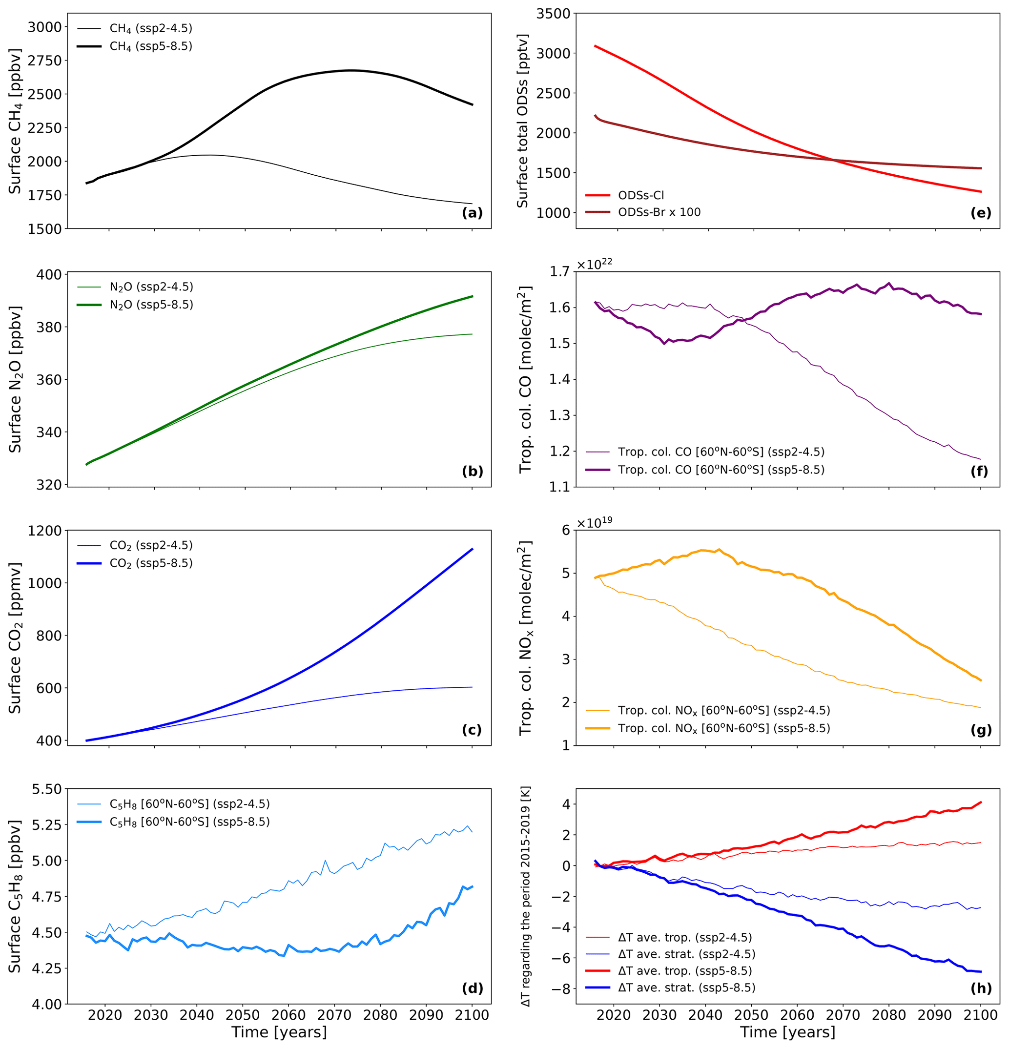
Figure 1 Annual mean evolution of drivers of ozone changes between 2015 and 2099 from both SSP2-4.5 (faded lines) and SSP5-8.5 (bold lines) – ODSs are presented as a single line, since their amounts are identical in both considered scenarios. This includes (a) global surface methane (CH₄) concentration [ppbv], (b) global surface nitrous oxide (N₂O) concentration [ppbv], (c) global surface carbon dioxide (CO₂) concentration [ppmv], (d) near-global (60^∘ N–60^∘ S) surface isoprene (C₅H₈) concentration [ppbv], (e) surface total organic chlorine (red line) and bromine (×100; dark-red line) ODS concentrations [pptv], (f) near-global (60^∘ N–60^∘ S) tropospheric carbon monoxide (CO) column [molec. cm⁻²], (g) near-global (60^∘ N–60^∘ S) tropospheric nitrogen oxide (NO_x) column [molec. cm⁻²], and (h) global mean changes in averaged tropospheric (red line) and averaged stratospheric (blue line) temperature (ΔT) regarding its mean for the period 2015–2019.

3.2 Ozone anomalies for the period 2015–2099 relative to the present-day ozone concentration

Figure 2 shows the annual mean partial and total column ozone changes in the near-global region throughout the 21st century with respect to the period 2015–2019 in different atmospheric layers. We calculated changes in O₃ relative to the period 2015–2019 to estimate the future modeled ozone change regarding its current concentration. It was noted that the evolution of tropospheric ozone is largely determined by changes in CH₄, CO, and NO_x (see Fig. 1). The contribution of CO seems to play a larger role in both scenarios, which might be due to less abundant NO_x. Nevertheless, in SSP5-8.5, the sharp decrease in O₃, starting after 2065, resulted mainly from the decrease in NO_x, as both CH₄ and CO start to decrease later. On the other hand, the projected sharp decline in NO_x makes CO a more important driver of tropospheric-ozone evolution in the last part of the century, especially under SSP5-8.5. Note that the decline in tropospheric-ozone concentration in SSP2-4.5 starts in the 2030s, much earlier than in SSP5-8.5. A steady increase in tropospheric ozone in SSP5-8.5 is observed by the 2060s; afterwards, it starts to sharply decrease during the last decades of the century, similarly to the RCP6.0 scenario (Revell et al., 2015b). Albeit, in the late century, tropospheric ozone will be lower than it is now in both scenarios – the difference in the zero-crossing point time is about 50 years between scenarios. In SSP2-4.5, the tropospheric-ozone concentration already becomes lower than the present-day one after 2050, while in SSP5-8.5, it is lower only around the end of the century.

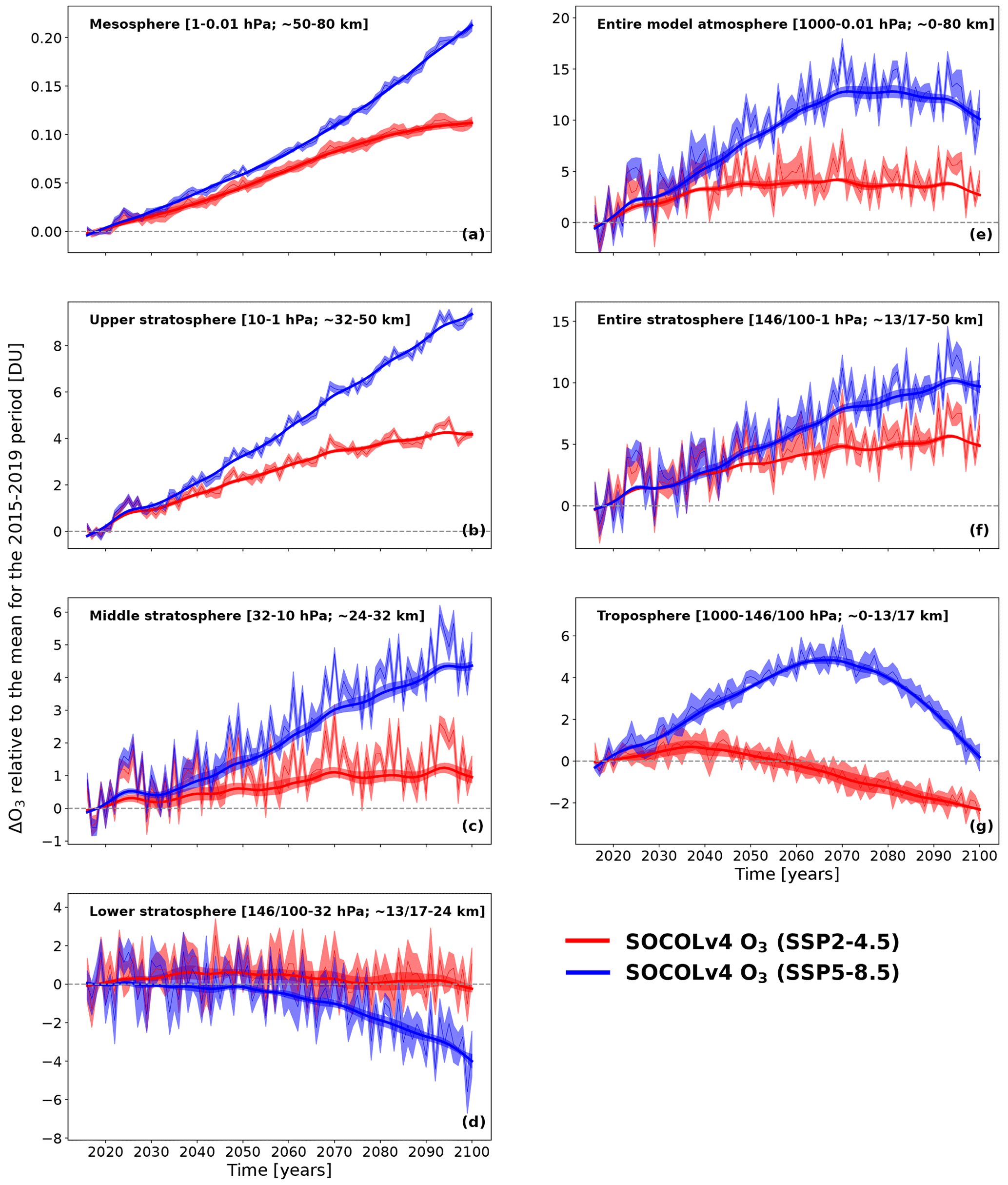
Figure 2 Near-global (60^∘ N–60^∘ S) annual mean anomaly (ΔO₃) of column ozone and DLM fits (both in Dobson units – DU) between 2015 and 2099, presented regarding the O₃ mean for the 2015–2019 period. The red line indicates ΔO₃ under the SSP2-4.5 scenario; the blue line indicates ΔO₃ under the SSP5-8.5 scenario. ΔO₃ is presented for (a) the mesosphere, (b) the upper stratosphere, (c) the middle stratosphere, (d) the lower stratosphere, (e) the entire model atmosphere, (f) the entire stratosphere, and (g) the troposphere. Shadings represent the 1σ standard deviation between ensemble members of the experiment.

The lower-stratospheric ozone on a near-global scale shows signs of a slight increase until the mid-century in SSP2-4.5. However, over the last half of the century, it began to gradually decline, showing a moderate reduction of about −1 DU (Dobson units) by 2099. In SSP5-8.5, the gradual decrease in ozone is visible during the whole considered period, showing a decrease of about −4 DU by the end of the century. In fact, this ozone decrease is mainly induced by the intensification of transport from the tropics toward the mid-latitudes. In addition, the decline in averaged ozone over 60^∘ N–60^∘ S indicates that the tropical ozone decrease in the lower stratosphere starts to prevail over the ozone recovery from the effects of hODSs on a near-global scale, as seen in Fig. 2. In contrast, increased NO_x might still contribute to ozone production in the lower stratosphere via smog reactions (e.g., Wang et al., 1998), and when it starts to decline, the ozone abundance also decreases more strongly. It should be also mentioned that the expansion of the ozone hole in SOCOLv4 is larger than in observations (see Sukhodolov et al., 2021), and the near-global averaged future ozone decline in the lower stratosphere can be slightly underestimated. In the middle and upper stratosphere, ozone recovers throughout the period due to a decline in hODS level, with a growth of 1 DU (in the middle stratosphere) and 4 DU (in the upper stratosphere) according to SSP2-4.5 and about 4.5 DU (in the middle stratosphere) and 9 DU (in the upper stratosphere) according to SSP5-8.5 by the end of the century. In SSP5-8.5, a much more intense growth after the 2040s is observed when the discrepancy in CO₂ evolution between scenarios becomes larger (see Fig. 1); i.e., the stratospheric temperature is lower in SSP5-8.5. In both scenarios, the evolution of the near-global averaged mesospheric ozone also increases. By the end of the century, the ozone content in the mesosphere will be higher than its modern level by ∼ 0.12 DU under SSP2-4.5 and by ∼ 0.22 DU under SSP5-8.5. This larger ozone enhancement in SSP5-8.5 might be due to lower temperatures and some influence of decreasing NO_x in the mesosphere. The total ozone column in SSP2-4.5 increases until the mid-century, after which it starts to slowly decline. In SSP5-8.5, the sharp increase in total ozone column transitions into a gradual decrease after the 2060s, which correlates well with the timing of both the sharp decline in tropospheric ozone and the intensification of the ozone decrease in the lower stratosphere. Even so, extra-polar mean total column ozone content by the end of the century will definitely be higher than present, wherein the magnitude of the increase is ∼ 2 to 3 times higher in SSP5-8.5 than in SSP2-4.5, which agrees well with previous studies (e.g., Keeble et al., 2021).

3.3 Ozone and driver trends development during the period 2015–2099

The understanding of ozone evolution requires knowing the changes in the driving agents such as temperature and important gas species involved in the ozone production and destruction cycles. The evolution of the CO, NO_x, temperature, and O₃ trends between 2015 and 2099 from both experiments is presented in Fig. 3.

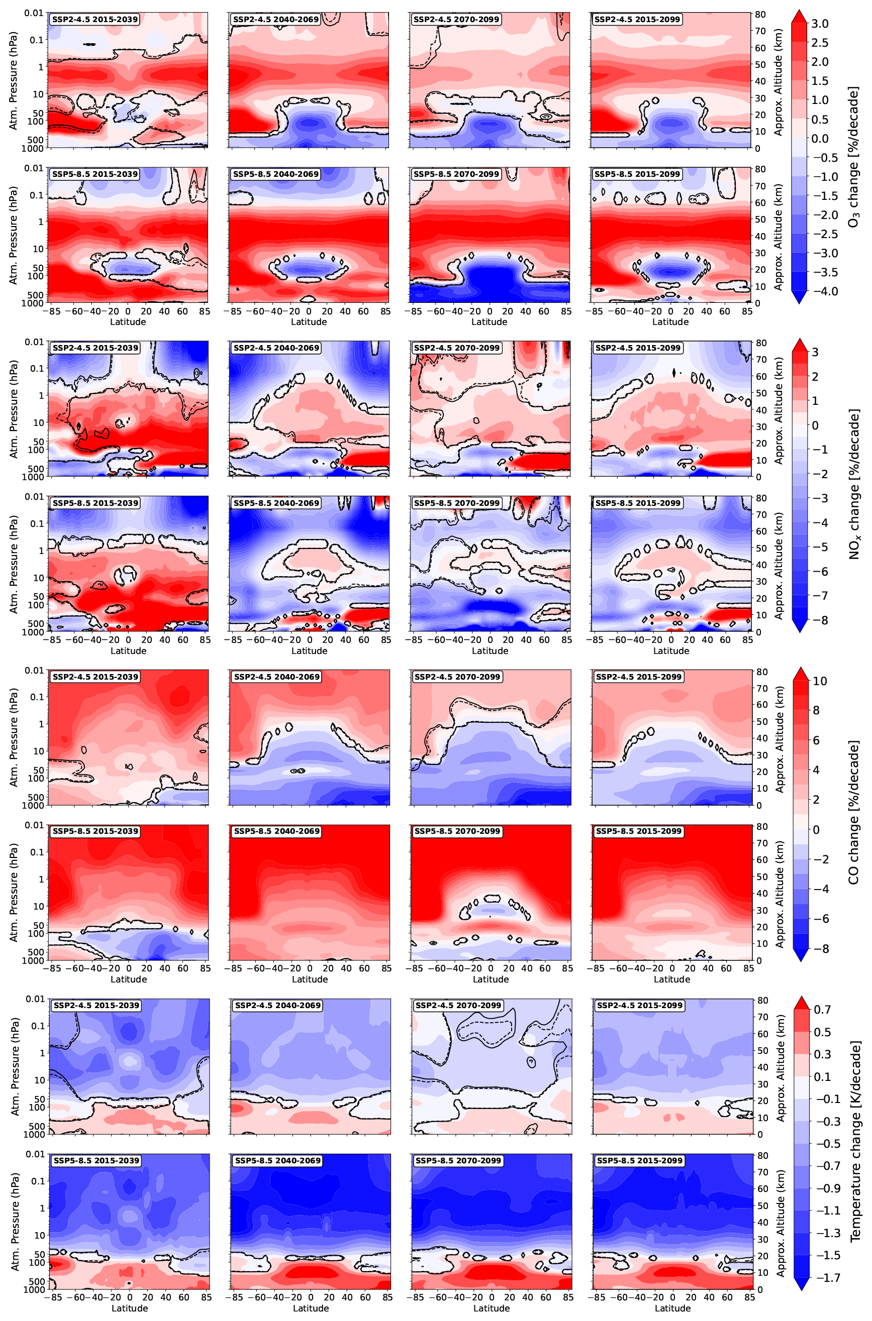
Figure 3 Profiles of trends in O₃, NO_x, CO, and temperature for the 2015–2099 period and different subperiods from both SSP2-4.5 and SSP5-8.5 simulations. The names of the corresponding scenario and the period are indicated in the upper left corner of each panel. The dashed line is the delimiter of the region, with significance at the 90 % level for positive or negative changes; the solid line is the same at the 95 % level.

Carbon monoxide is produced via CO₂ photolysis by solar irradiance in the upper atmosphere (e.g., Thompson et al., 1963; Solomon et al., 1985) and can be transported downward, mostly over the high latitudes during cold seasons. Therefore, its abundance in these areas strongly reflects CO₂ behavior, mimicking a steady increase in SSP5-8.5 and stabilization in SSP2-4.5. The increase in CO in the stratosphere should not strongly contribute to the ozone changes; however, some slight effect can be expected from the removal of OH caused by the CO + OH → CO₂ + H reaction (Wofsy et al., 1972). In the troposphere, the CO source is driven by methane and biogenic volatile organic compounds (VOCs). Therefore, we observe a steady CO decline after 2040 in SSP2-4.5 following the drop in methane emissions (see Fig. 1). For the SSP5-8.5, the change of signs appears in 2070 after flattening and a small decline of the methane mixing ratio. An initial negative tendency for the 2015–2039 subperiod is related to a small decrease in VOCs. The CO tendencies in the stratosphere are defined by the upward transport and mixing of the tropospheric air. Carbon monoxide can be considered as a proxy for the level of organic species, which are a necessary part of the tropospheric-ozone production mechanism. The concentration of NO_x is the second part participating in this process.

In the mesosphere, NO_x (NO + NO₂) is mostly produced by N₂O oxidation, energetic particles, and influx from the thermosphere. They can be destroyed by solar irradiance via NO₂ photolysis followed by a cannibalistic N + NO → N₂ + O reaction. Because the thermospheric source is the same for both cases and is partly accounted for by solar proxies, the NO_x trend in the mesosphere depends on the available N₂O and temperature, which regulate the efficiency of the cannibalistic reaction, making it faster for the cooler environment in the future. Despite a steady N₂O increase (see Fig. 1), the N₂O in the mesosphere is less available due to its higher destruction by enhanced ozone and O(¹D) concentration in the stratosphere. Thus, less N₂O abundance and cooler temperature lead to a general decrease of the mesospheric NO_x. For the 2070–2099 subperiod, however, the NO_x depletion for the SSP2-4.5 case is not so pronounced due to mesospheric cooling that is probably very small.

Stratospheric NO_x concentration is mostly regulated by the production via N₂O + O(¹D) → NO + NO and the conversion to reservoir species, which depend on the temperature and availability of hydrogen- and halogen-containing species, which deactivate NO_x-building reservoir species like HNO₃ or ClONO₂. Therefore, the stratospheric NO_x increase is more substantial in the SSP2-4.5 case when the cooling and water vapor increases are not so pronounced as in the SSP5-8.5 case (see Keeble et al., 2021 for trends in H₂O).

NO_x mostly declines in the lower troposphere due to improved air quality. Also, most periods in both scenarios show the permanent increase in free tropospheric NO_x over the Northern Hemisphere's upper troposphere, which is maintained by aircraft emissions.

The temperature trend patterns look as expected (e.g., IPCC, 2021). A continuous increase of greenhouse gases leads to tropospheric warming and stratospheric cooling (e.g., Lee et al., 2021), and both are substantially more pronounced in the SSP5-8.5 scenario due to more intensive anthropogenic activity. The tropospheric warming in this case is more prominent over the Northern Hemisphere due to Arctic amplification (e.g., Previdi et al., 2021) and in the lower stratosphere over the southern high latitude, where the ozone concentration is increasing due to the recovery from the halogen loading to pre-ozone hole conditions. The radiative cooling by greenhouse gases dominates in the stratosphere in relation to some warming caused by the stratospheric-ozone increase, and it agrees with the time evolution shown in Fig. 1. During the first 2015–2039 subperiod, the quadrupole structure of stratospheric temperature trends is observed in both scenarios, which is dynamically induced (Ball et al., 2016) and is barely observed in later subperiods.

The ozone change patterns substantially differ between layers. In the troposphere, the ozone decrease is observed for the SSP2-4.5 scenario starting from 2040, as well as for the entire period. This behavior is explained by the continuous decrease of the ozone precursors related to the improvement of air quality. For the SSP5-8.5, a similar process occurs only after 2070 when the NO_x atmospheric abundance decline, together with the decline in CO, is the most prominent (see Fig. 1g). A similar decrease in the tropospheric ozone resembles the results obtained by Revell et al. (2015b) using the RCP6.0 scenario. Some increase in NO_x level before 2070 leads to positive tropospheric-ozone trends, which makes the ozone trend positive for the entire period. The pattern and magnitude of obtained statistically significant tropospheric-ozone trends over the entire period are consistent with those in the multi-model mean given in Keeble et al. (2021) and for WACCM and IPSL models from Shang et al. (2021) for corresponding SSP scenarios.

In the upper stratosphere and southern lower stratosphere, the ozone increase is very persistent because it is driven by a steady decline of the halogen loading (see Fig. 1). The ozone increase in the upper stratosphere is stronger for the SSP5-8.5 case because a more pronounced stratospheric cooling leads to less intensive catalytic ozone destruction cycles. Another area with a persistent trend appears in the tropical lower stratosphere, where intensification in the warmer-climate Brewer–Dobson circulation drives negative ozone trends (e.g., Zubov et al., 2013). This feature is more pronounced for the SSP5-8.5 scenario after 2070 because of the stronger warming. Before 2070 and for the entire period, the magnitude of the ozone decline in this area is virtually the same for both cases due to compensation of the dynamical loss by means of increased tropospheric ozone obtained for SSP5-8.5. Overall, stratospheric-ozone trends are mostly statistically significant for the entire period and are consistent with previous findings (Keeble et al., 2021; Shang et al., 2021). In MRI-ESM2, the pattern of future ozone trends (see Shang et al., 2021) differs from that modeled with SOCOLv4, but this was anticipated due to limitations identified in MRI-ESM2 (Keeble et al., 2021).

In the upper mesosphere, ozone decreases until 2070 under SSP5-8.5 due to an increase in CH₄ causing an increase in mesospheric abundance of H₂O and, hence, an enhancement of HO_x radicals. Under SSP2-4.5, mesospheric ozone has generally increased over the entire period of 2015–2099, since CH₄ only increases slightly until the 2040s and then begins to decline.

3.4 Total column ozone trend development during the period 2015–2099

One way or another, changes in ozone in different layers of the atmosphere contribute to a change in total column ozone. It is essential for humanity to know the future evolution of total ozone because it affects changes in ground-level UV radiation. Figure 4 shows the evolution of trends in total column ozone as a function of month and latitude over the period 2015–2099 and intermediate subperiods.

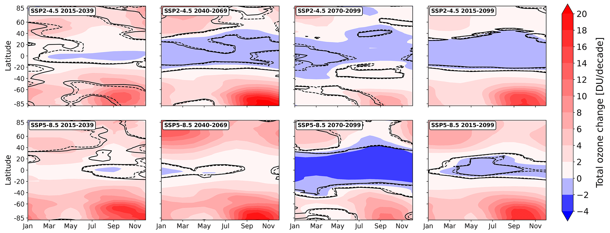
Figure 4 Trends in total column ozone as a function of month and latitude for the 2015–2099 period and different subperiods from both SSP2-4.5 and SSP5-8.5 simulations. The names of the corresponding scenario and the period are indicated in the upper left corner of each panel. The dashed line is the delimiter of the region, with significance at the 90 % level for positive or negative changes; the solid line is the same at the 95 % level.

The total ozone recovery in austral spring over the Southern Hemisphere is generally similar between both scenarios, since it is driven by the phase-out of hODSs emissions, which are identical in both scenarios. However, the ozone increase is slightly higher in SSP5-8.5 owing to a lower temperature in the stratosphere. It is also seen that, during 2070–2099, in both scenarios, the ozone increase is slowed down. This might be because of the slower hODS decline and the GHG increase (see Fig. 1) and due to the contribution of tropospheric-ozone decline (see Fig. 2). In mid-latitudes, the ozone increase is also higher in SSP5-8.5 due to both temperature and more intense transport from the tropics. In contrast, in the tropics, trends in total ozone largely differ between scenarios. In SSP2-4.5, the tropical total ozone tends to reduce during the entire period by about −2 DU per decade due to ozone decreases in the lower stratosphere and troposphere. A strong decline in total ozone of about −4 DU per decade between 2070 and 2099 is observed in SSP5-8.5, but in other subperiods, the trend in tropical total column ozone is generally near zero due to an increase in tropospheric ozone that partly compensates for the ozone decline in the lower-stratospheric ozone. During boreal spring, the total ozone also increases in the Northern Hemisphere in both scenarios, with a higher increase in SSP5-8.5. The presented statistically significant total ozone column change distributions for the entire 2015–2099 period are highly compatible with the multi-model mean given in Keeble et al. (2021) for both considered SSP scenarios.

Thus, some increase in surface UV level over the tropics and a decrease over the middle and high latitudes can be expected in both scenarios, but in SSP2-4.5, it will be higher in the tropics throughout the entire period, while in SSP5-8.5, it will be higher in the late century only. On the contrary, the decrease in surface UV level at middle and high latitudes is expected to be greater in SSP5-8.5 than in SSP2-4.5 due to higher ozone.

4 Discussion and conclusions

In this paper, we have evaluated atmospheric-ozone trends based on two sets of ensemble simulations using SOCOLv4, covering the period from 2015 to 2099. One simulation is based on the SSP2-4.5 scenario, and the other is based on the SSP5-8.5 scenario; these scenarios differ in terms of greenhouse gas emissions and ozone precursors. The trends in ozone, as well as in non-hODS drivers of ozone evolution such as NO_x, CO, and temperature, are derived using DLM. The ozone layer is expected to increase on a near-global scale throughout the entire century because of the ban on the production of hODSs by the Montreal Protocol. However, the evolution of atmospheric ozone in different atmospheric layers differs greatly between the two SSP scenarios. The tropospheric-ozone evolution, driven mainly by CO and NO_x changes, shows a difference in the time of inflection point when tropospheric ozone begins to decline. In SSP2-4.5, it began to be observed after 2040, while in SSP5-8.5, it began to be observed after 2065. In the mesosphere and the upper and middle stratosphere, a resilient increase in ozone is about 2 to 3 times higher in SSP5-8.5 than in SSP2-4.5, since the negative temperature trends in these regions in SSP5-8.5 are more than 1 K per decade stronger, which retards the catalytic ozone loss. In the lower stratosphere, the near-global ozone content tends to decline after 2040 in SSP2-4.5 and during the whole considered period in SSP5-8.5; by the end of the century, the decrease in SSP5-8.5 is more than 3 times higher due to faster meridional transport of ozone to the poles. The obtained ozone trends for different regions are consistent with those presented in previous studies (Keeble et al., 2021; Shang et al., 2021).

In general, it is difficult to establish trends in ozone in the extratropical lower stratosphere due to the large uncertainty associated with natural variability (Ball et al., 2018). However, for the long-term periods, statistically robust projection in this part of the atmosphere is possible, as we show in this study. In addition, there are other factors which might contribute to the uncertainty of future ozone evolution. For instance, we have no future volcanic activity considered in our study because it is hard to predict volcanic eruptions. However, severe implications for the ozone layer in the future are expected if strong volcanic eruptions occur (Klobas et al., 2017). In addition, no less important for the future ozone evolution might be the projected decline in solar activity throughout the 21st century (Steinhilber and Beer, 2013; Matthes et al., 2017), which also has not been considered in our study. Yet, it is well known that solar activity mainly drives photochemical and dynamical processes in the stratosphere and is responsible for the ozone formation and radiation budget (Haigh, 1994; Rozanov et al., 2004; Hood and Soukharev, 2003; Egorova et al., 2004). Therefore, a decline in solar activity might lead to a decrease in atmospheric-ozone production, causing some negative implications for its future evolution (Anet et al., 2013; Rozanov et al., 2016; Arsenovic et al., 2018).

Nevertheless, total column ozone is expected to increase almost everywhere, except in the tropics. In both polar regions, the total ozone increases with a slightly higher intensity in SSP5-8.5. In the mid-latitudes, the total ozone also increases thanks to the upper-stratospheric-ozone increase and transport from the tropics. Conversely, in the tropics, it generally declines in SSP2-4.5 due to both tropospheric- and lower-stratospheric-ozone decreases, equating to about −2 DU per decade; it changes in SSP5-8.5, with a sharp decrease of about −4 DU per decade only during the last decades of the century due to a severe reduction in both tropospheric- and lower-stratospheric-ozone content. We showed that, besides changes in the stratospheric-ozone column, it is also essential to consider the tropospheric column ozone evolution, since it may seriously contribute to total column ozone evolution, especially in the tropics.

A much stronger ozone increase in the upper part of the middle atmosphere and the middle to high latitudes of the lower stratosphere might also be expected in the SSP5-8.5 scenario. In this regard, it may seem that the more-greenhouse-gases scenario is better because, despite higher near-surface temperatures, it will be more favorable for ozone increases over the most populated areas. However, the excessive increase in ozone over middle to high latitudes may also have negative consequences for human well-being. Exceeding the required level of total ozone content, especially over the most inhabited areas, means more UV absorption and, consequently, less surface-level UV radiation than what is required for human health. It causes less vitamin D synthesis and therefore increases the risk of diseases related to vitamin D deficiency, like rickets and osteomalacia (Butler et al., 2016). In addition, it is worth paying attention to the evolution of ozone in the tropics. There is a risk of a decrease in total ozone content, leading to an increase in surface UV level abnormalities, which also has negative effects on human health, like an increased risk of skin cancer and cataracts (Butler et al., 2016).

The important message in this regard is to find a way to bring the ozone content in the atmosphere to an equilibrium state, where it is neither lower nor higher than necessary. Thus, we emphasize that the findings presented in this study will be useful for further improvement of socioeconomic-pathway policies to determine the route to maintain the global total ozone content that is favorable for the sustainable development of human civilization.

Appendix A

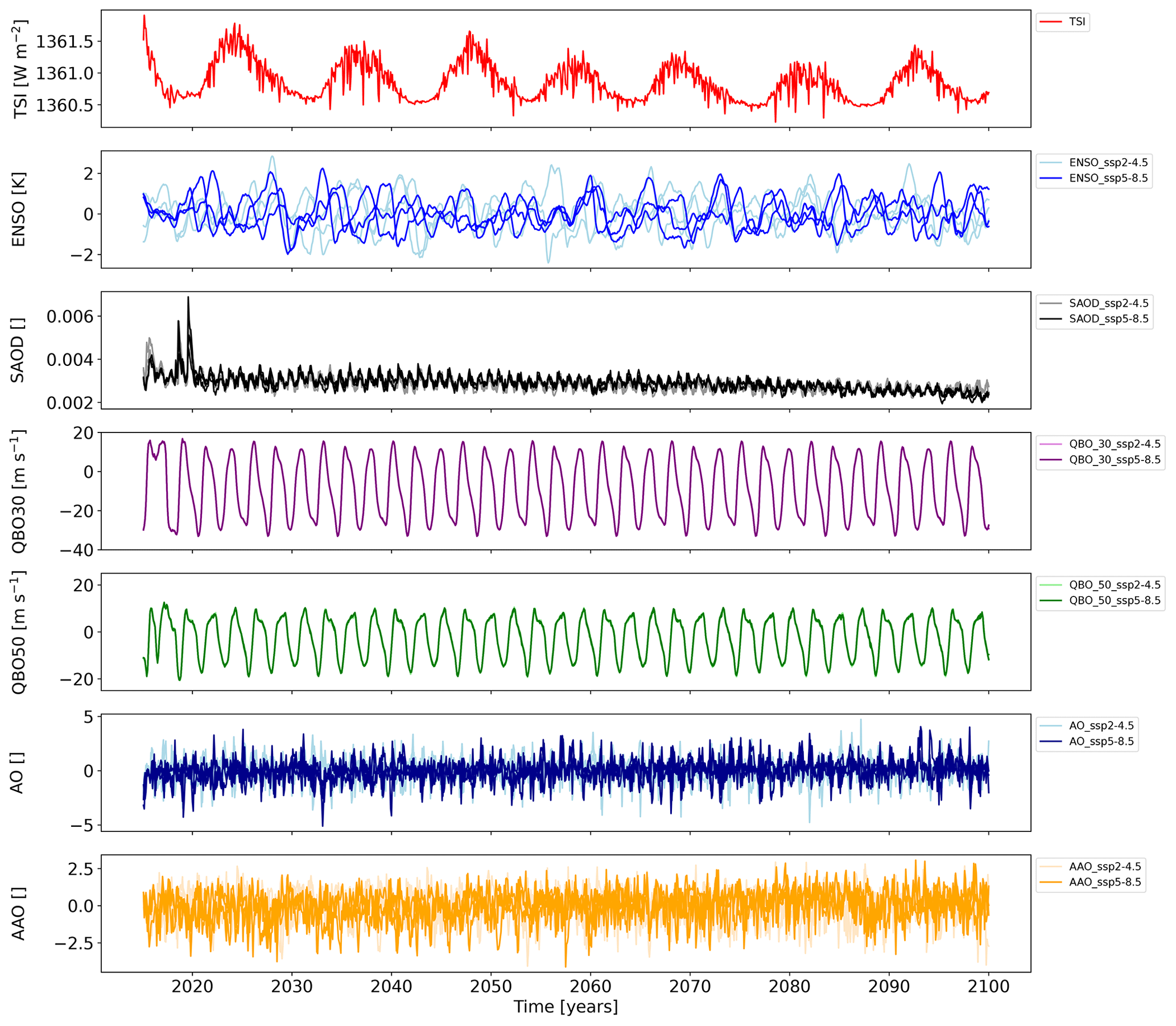
Figure A1 Input quantities (proxy variables) for the forcing of the SOCOLv4 simulations. Faded colors are for SSP2-4.5; bright colors are for SSP 5-8.5.

Figure A2 Pearson’s linear correlation coefficients for different covariate variables (proxy variables) of the SOCOLv4 simulations for the 2015–2099 period: (a) for SSP2-4.5 and (b) for SSP5-8.5. Error bars represent the 1σ standard deviation of the correlation coefficients between ensemble members.