Impacts of land cover changes on biogenic emission and its contribution to ozone and secondary organic aerosol in China

The greening impacts on China from 2000 to 2017 led to an increase in vegetated areas and thus enhanced biogenic volatile organic compound (BVOC) emissions. BVOCs are regarded as important precursors for ozone (O₃) and secondary organic aerosol (SOA). As a result, accurate estimation of BVOC emissions is critical to understand their impacts on air quality. In this study, the Model of Emissions of Gases and Aerosols from Nature (MEGAN) v2.1 was used to investigate the impact of different leaf area index (LAI) and land cover (LC) datasets on BVOC emissions in China in 2016, and the effects on O₃ and SOA were evaluated based on the Community Multiscale Air Quality (CMAQ) modeling system. Three LAI satellite datasets of the Global LAnd Surface Satellite (GLASS), the Moderate Resolution Imaging Spectroradiometer (MODIS) MOD15A2H version 6 (MOD15), and the Copernicus Global Land Service (CGLS), as well as three LC satellite datasets of the MODIS MCD12Q1 LC products, the Copernicus Climate Change Service (C3S) LC products, and the CGLS LC products, were used in five parallel experiments (cases: C1–C5). Results show that changing LAI and LC datasets of the model input has an impact on BVOC estimations. BVOC emissions in China ranged from 25.42 to 37.39 Tg in 2016 and were mainly concentrated in central and southeastern China. Changing the LC inputs for the MEGAN model has a more significant difference in BVOC estimates than using different LAI datasets. The combination of C3S LC and GLASS LAI performs better in the CMAQ model, indicating that it is the better choice for BVOC estimations in China. The highest contribution of BVOCs to O₃ and SOA can reach 12 ppb and 9.8 µg m⁻³, respectively. Changing the MEGAN inputs further impacts the concentrations of O₃ and SOA, especially changing LC datasets. The relative difference between MCD12Q1 LC and C3S LC is over 52 % and 140 % in O₃ and biogenic SOA (BSOA) in central and eastern China. The BSOA difference is mainly attributed to the isoprene SOA (ISOA), a major contributor to BSOA. The relative differences in ISOA between different cases are up to 160 % in eastern China. Therefore, our results suggest that the uncertainties in MEGAN inputs should be fully considered in future O₃ and SOA simulations.

1 Introduction

Volatile organic compounds (VOCs) from both natural and anthropogenic sources play important roles in the formation of ozone (O₃) and secondary components of fine particulate matter (PM_2.5) in addition to their adverse health effects (Volkamer et al., 2006; Laothawornkitkul et al., 2009; Calfapietra et al., 2013; Zhao et al., 2021). Globally, biogenic VOCs (BVOCs) from vegetation are the dominant contributor (with ∼ 90 % contribution) to VOCs (Fehsenfeld et al., 1992; Guenther et al., 1995). Isoprene, monoterpenes, and sesquiterpenes are major BVOC species (Guenther et al., 2006; H. Wang et al., 2018) with high photochemical reactivity with O₃, hydroxyl radical (OH), and nitrate radical (NO₃). In addition, changes in BVOC emissions also apparently alter the concentrations of key pollutants that affect the climate. In particular, O₃ and CH₄ can warm the climate, while the aerosols (organics, sulfate, and nitrate) have a cooling effect by scattering solar radiation (Unger, 2014a, b). Consequently, studies on BVOC emissions and their effects on air quality and climate are of vital significance.

The Model of Emissions of Gases and Aerosols from Nature (MEGAN) is a widely used (Guenther et al., 2012; Zhao et al., 2016; Emmerson et al., 2018) model to quantify BVOC emissions at different spatial scales (Guenther et al., 1995; Sindelarova et al., 2014; Zhang et al., 2017; Jiang et al., 2019; Wang et al., 2021). Global annual inventories of the isoprene emission range from 500 to 750 Tg yr⁻¹ (Guenther et al., 2006) and those of monoterpene emissions range from 74.4–157 Tg yr⁻¹ (Guenther et al., 2012; Messina et al., 2016). BVOC emissions have also been estimated in China by various studies, and the results showed that isoprene emissions were 7.17–29.30 Tg yr⁻¹, and monoterpene emissions were 2.83–5.60 Tg yr⁻¹ (Guenther et al., 2006; Fu and Liao, 2012; Li et al., 2020). The model determined the vegetation types according to model inputs and then used the activity factor multiplied with the emission factor to calculate emissions for each vegetation type (Guenther et al., 2012). However, there are considerable uncertainties in BVOC estimations due to incomplete information on model inputs, activity factors, and emission factors (Situ et al., 2014; Guenther et al., 2012). Those factors can influence the accuracy of estimations and further result in uncertainties of O₃ and SOA. Therefore, it is necessary to quantify the influence of those factors and to determine the bias in BVOC emissions.

Land cover (LC), including leaf area index (LAI) and plant function type (PFT) fractions, is a major factor affecting the BVOC emissions in the MEGAN model (Guenther et al., 2006; Pfister et al., 2008; Guenther et al., 2012). There are many LAI and LC products generated by various satellite sensors with different process methods and spatial and temporal resolutions. These products show discrepancies in biomass distributions and PFT fractions, which can increase bias in BVOC estimations (Leung et al., 2010; Y. Wang et al., 2020; Opacka et al., 2021). Guenther et al. (2006) reported that differences in isoprene emissions could be 24 % and 29 % due to changing PFTs and LAI, respectively. Pfister et al. (2008) found that differences in BVOC emissions were more significant on a regional scale than a global scale by employing three different PFT and LAI databases to drive the MEGAN model. H. Wang et al. (2018) showed that the differences in BVOC estimations were 35.5 % and 22.8 % as a result of changing PFTs and LAI, respectively. China is globally a typical greening country with a forest area of 22.96 % in 2018 (SFA, 2019), contributing large annual BVOC emissions to the world (Opacka et al., 2021), and thus reasonable comparisons in LAI and LC satellite products are essential for a better understanding of BVOC emissions from China.

Contributions of BVOCs to surface O₃ and SOA have been evaluated through chemical transport models (CTMs) at different spatial scales (Carlton and Baker, 2011; Fu and Liao, 2014; Jiang et al., 2019; Zhang et al., 2020). Fu and Liao (2012) used the Goddard Earth Observing System chemical transport model (GEOS-Chem) to quantitate the impact of biogenic emissions on O₃ in China over the years 2001–2006 and found that the difference in O₃ concentrations induced by interannual variability of BVOCs could be 2 %–5 %. Based on the Weather Research and Forecasting model coupled with Chemistry (WRF-Chem), Situ et al. (2013) reported that about 57 % higher O₃ formed from isoprene in urban areas than in rural areas in the Pearl River Delta (PRD). In addition to the impact on surface O₃, Wu et al. (2020) studied the contributions of BVOCs to SOA in China in 2017 by using the Community Multiscale Air Quality (CMAQ) model, and the result indicated that BVOCs are the main source of the formation of SOA in summer, which was up to 70 %. Qin et al. (2018) investigated the biogenic SOA (BSOA) during summertime in 2012 and found that a high level of BSOA concentration appeared in the Sichuan Basin. However, previous studies have only focused on the impacts of BVOCs estimated by the specific LAI and LC satellite products on air quality. The uncertainties in BVOC estimations induced by different satellite products also have an impact on O₃ and SOA concentrations. Kim et al. (2014) showed that the different PFT distributions had a significant impact on hourly and local O₃, which was up to 13 ppb. Y. Wang et al. (2020) evaluated that the impacts on O₃ reached 20 % by using different LC datasets in BVOC emissions in the Yangtze River Delta (YRD). The influence of these uncertainties on air quality was not well quantified, and the bias in the air quality remained unclear in China. Therefore, it is necessary to conduct a comprehensive analysis of the influence of different satellite products on BVOC emissions as well as the further impact on air quality.

In this study, the objectives are to estimate the difference in BVOC emissions induced by different LAI and LC databases in China and to study the effects of differences in BVOC emissions on surface O₃ and SOA concentration in China. We used three LAI satellite datasets and three LC satellite datasets as the MEGAN v2.1 inputs to estimate the BVOC emissions and then determined their impacts on air quality by using a source-oriented model. Section 2 introduces the MEGAN model, the source-oriented CMAQ model, and datasets. The model performance, BVOC estimations based on different satellite products, as well as the impact of BVOCs on atmospheric pollutants, are described in Sect. 3, while Sect. 4 concludes the study.

2 Methodology

2.1 Model setup

An updated source-oriented CTM was applied to determine O₃ and SOA concentrations from BVOCs based on the CMAQ model v5.0.1 (Byun and Schere, 2006). The model utilizes a revised State-wide Air Pollution Research Center version 11 (SAPRC-11) photochemical mechanism (S11) (Carter and Heo, 2013), which includes a more explicit description of isoprene oxidation chemistry to improve isoprene aerosol predictions (Ying et al., 2015). Changes in the SOA module includes the surface uptake of dicarbonyls and isoprene epoxides, as well as predictions of glyoxal and methylglyoxal (Ying et al., 2015). The aerosol yields are updated to account for vapor wall loss during chamber experiments as described by Zhang et al. (2014). The S11 gas-phase mechanism and the SOA module are further expanded with a precursor tracking scheme to track emissions from different sources separately so that the formation of SOA can be determined. The complete description of SOA source tracking has been described by Zhang and Ying (2011) and P. Wang et al. (2018), and a brief introduction is described below.

The modified S11 mechanism expands the specific original reactions into two sets of similar reactions to track the formation of O₃ and SOA. The concentrations of O₃ from different VOC sources (henceforth O₃_VOC_i) were determined by the source-oriented method (Ying and Krishnan, 2010). Based on the method, the non-reactive O₃ tracer is used to track O₃ attributed to BVOCs, which is tagged as O₃_VOC_bio and directly predicted. The descriptions of O₃ source apportionment are detailed in Wang et al. (2019). As for SOA, the specific source x (for instance, biogenic source) is tracked by adding a superscript x on the precursors related to SOA (like TERP, the abbreviation of monoterpene in the S11 photochemical mechanism) and their products, while the contributions from all other sources are simulated based on none-tagged TERP. The tagged species TERP^x reacts with OH to form the primary product TRPRXN^x, which is the counterspecies for the aerosol precursor from monoterpenes and subsequently formed semi-volatile oxidation products SV_TRP1^x and SV_TRP2^x based on the two-product approach and thus determines the fine-mode SOA species ATRP1^x and ATRP2^x due to gas-to-particle partitioning. By considering those species with the superscript x, it is possible to track the SOA formed by the ATRP of source x. The contributions of other precursors of SOA are calculated using the same approach.

The WRF model v3.6.1 was used to generate meteorological conditions for MEGAN and CMAQ. The modeling domain in WRF was 36 km × 36 km in horizontal spatial resolution, which covers China and its surrounding countries in East Asia (Fig. S1 in the Supplement) (Zhang et al., 2012). The boundary and initial conditions applied in WRF were from the National Centers for Environmental Prediction (NCEP) Final (FNL) Operational Model Global Tropospheric Analyses dataset (available at http://rda.ucar.edu/datasets/ds083.2/, last access: 18 May 2022). The model configurations are similar to that of the previous studies (P. Wang et al., 2018, 2020; Zhu et al., 2021), and Table S1 briefly lists the physical options used for the WRF model. MEGAN v2.1 was applied to estimate 19 compound classes of BVOCs (Guenther et al., 2012). In MEGAN, the LC and LAI datasets in 2016 were used and then were gridded to the same spatial resolution to generate PFT fractions and LAIv (the LAI of vegetation-covered surfaces) maps as inputs for the model. The CMAQ model used the same horizontal resolution as WRF with a horizontal domain of 197 × 127 grid cells. This domain covers China and its surrounding areas (Fig. S1). The meteorological conditions as inputs to the CMAQ model were provided by the WRF model v3.6.1. The anthropogenic emissions of China used the datasets from the Multi-resolution Emission Inventory for China (MEIC; available at http://www.meicmodel.org, last access: 3 May 2022). Since the MEIC only provides anthropogenic emissions for China, anthropogenic emissions from foreign countries were provided by the Emissions Database for Global Atmospheric Research (EDGAR) v4.3 (available at http://edgar.jrc.ec.europa.eu/overview.php?v=_431, last access: 10 May 2022). The MEIC inventory is widely used in air quality studies in China (M. Li et al., 2017; Hu et al., 2016; Wu et al., 2020). It was improved in a vehicle emission inventory with high resolution (Zheng et al., 2014) and a non-methane VOC mapping approach for different chemical mechanisms (Li et al., 2014). EDGAR is a gridded emission inventory with a high horizontal resolution of 0.1^∘ × 0.1^∘ (Saikawa et al., 2017).

2.2 Data description

LAI and PFTs are key parameters for BVOC estimations. Three LC datasets were applied as PFT inputs, including the Moderate Resolution Imaging Spectroradiometer (MODIS) MCD12Q1 LC products (Friedl and Sulla-Menashe, 2019), the Copernicus Climate Change Service (C3S) LC products (C3S, 2019), and the Copernicus Global Land Service (CGLS) LC products (Buchhorn et al., 2020). MCD12Q1 provides yearly global LC maps from 2001 to 2020 with a spatial resolution at 500 m, which has been widely used in previous studies (Guenther et al., 2006; H. Wang et al., 2018; Wu et al., 2020). Thus, MCD12Q1 is chosen as the baseline LC input for MEGAN v2.1 to investigate the model performance with different LAI satellite products. Sources of these products are listed in Table S2. PFTs used in the MEGAN model adopt the scheme used for the Community Land Model v4.0 (CLM4) (Guenther et al., 2012). Three LC maps are first regridded to the CMAQ domain (Fig. S2). Secondly, LC types are categorized into eight vegetation types according to legend descriptions of LC maps. Lastly, eight vegetation types are further reclassified into 15 CLM4 PFTs based on the climate rules described in Bonan et al. (2002). Figure 1 shows the simulation domain with the spatial distribution of major PFTs. The three datasets show a consistent distribution of grass in northwestern China, but they display distinct PFTs in central and southern China. Cropland is the dominant PFT in central and southern China in the C3S LC map. Although MCD12Q1 and CGLS LC both show a large area in central and southern China, the area fraction of the broadleaf tree in CGLS LC is higher than that in MCD12Q1 (Figs. 1 and S3).

Figure 1 Simulation domain with the spatial distribution of major PFTs in each grid.

Figure 2 Distribution of LAIv from different satellite datasets in the summer of 2016.

The Global LAnd Surface Satellite (GLASS) (Xiao et al., 2014, 2016), the MODIS MOD15A2H version 6 (MOD15) (Myneni et al., 2015), and the CGLS LAI products (Fuster et al., 2020) were applied as LAI inputs for MEGAN v2.1. The spatial resolutions of GLASS, MOD15, and CGLS are 500, 500, and 300 m, respectively, while the temporal resolutions of these three products are 8, 8, and 10 d, respectively. Sources of these products are listed in Table S2. According to validation results in Xiao et al. (2016), GLASS shows better consistency than MOD15 in high resolution in LAI maps, while CGLS is slightly less accurate than MOD15 (Fuster et al., 2020). Therefore, GLASS is used as the baseline LAI input. In the MEGAN model, the grid average LAI is divided by the fraction of the grid that is covered by vegetation to represent the LAI of vegetation-covered surface, which is referred to as LAIv (Guenther et al., 2006). Figure 2 represents the spatial distribution of LAI from three satellite datasets in the summer of 2016. The MOD15 LAI dataset used in C2 shows differences from C1, especially in southern China, where the GLASS LAIv is about 50 % higher than the MOD15 LAIv. The MOD15 LAIv is lower in the North China Plain (NCP) than in other products because the MOD15 underestimates the LAI of maize and wheat in NCP (Yang et al., 2015; Wang et al., 2022).

Table 1 Simulation schemes with different land cover (LC) and leaf area index (LAI).

Table 1 presents the setup of the simulation scenarios. Scenarios C1 to C3 use MCD12Q1 as the PFT input and different LAI inputs to investigate the effects of varied LAI datasets on BVOC emissions, while the impacts of different PFT maps on BVOC estimations are studied in scenarios C1, C4, and C5, which use GLASS as the LAI input. It should be noted that those experiments use the same meteorological conditions provided by the WRF model for BVOC estimations. Besides BVOC simulations, a 1-year CMAQ simulation with five different sets of MEGAN input data is conducted in the year 2016 in China with the same meteorological conditions and anthropogenic emissions to investigate the impacts of BVOCs on O₃ and SOA concentrations. It is worth noting that the meteorological conditions remain constant when simulating, and the model chemistry does not affect them.

3 Results and discussion

3.1 Model performance

Temperature (T2), relative humidity (RH), wind speed (WS), and wind direction (WD) at 10 m above the surface were compared to observations from the National Climate Data Center (NCDC, available at https://www.ncei.noaa.gov/access, last access: 13 May 2022). The statistical measures and results are shown in Tables S3 and S4, respectively. The T2 predictions for the entire year show a negative mean bias (MB) value, which is slightly lower than the benchmarks suggested by Emery et al. (2001). This is primarily due to the overestimation of cloud coverage in the WRF model, resulting in an underestimated T2 (Wu et al., 2020). Although biases exist in the T2 simulation, the yearly long WRF simulation in this study shows relatively small biases compared to previous studies (Wu et al., 2020; H. Wang et al., 2018), and the daily variation in temperature is successfully simulated for most cities in China (Fig. S4). The gross error (GE) values of WS are within the acceptable criteria of 2 for all seasons, but the WRF model still overpredicts the WS. The MB values of WD meet the benchmarks of ±10 in all seasons, indicating a good agreement between model predictions and observations. However, the GE values exceed the benchmarks of ±30. Moreover, the predicted RH in spring and winter shows a slight underestimation compared to observations, whereas in summer and fall it is overestimated. Generally, the performance of the WRF model in this study is comparable to previous studies (Hu et al., 2016; H. Wang et al., 2018; Wang et al., 2010; Ma et al., 2021). Therefore, the meteorological conditions predicted by the WRF model are acceptable inputs for the CMAQ model in follow-up research.

Hourly observations from the publishing website of the China National Environmental Monitoring Center (available at http://www.cnemc.cn/, last access: 4 May 2022) were used to validate the CMAQ model prediction of O₃ and PM_2.5. In order to investigate the impacts of varied total BVOC emissions on air pollutants, the model performance was evaluated separately for different cases. Table S5 presents the model performance statistics for maximum daily averaged 1 h (MDA1) O₃ and maximum daily averaged 8 h (MDA8) O₃ in 2016, including mean observations (OBS), mean predictions (PRE), mean fractional bias (MFB), mean fractional error (MFE), mean normalized bias (MNB), and mean normalized error (MNE). Cutoff concentrations of 60 ppb were used for MDA1 O₃ and MDA8 O₃ in this validation, which was suggested by the U.S. EPA (U.S. EPA, 2005). In general, the model performance of MDA1 O₃ and MDA8 O₃ in China, including its important regions, meets the model performance benchmarks suggested by the U.S. EPA (2005). The MNB values of MDA1 O₃ in China range from 0.02–0.05, which fall within the criteria of ±0.15. Similarly, the MNE values of MDA1 O₃ range from 0.18–0.19, which fall within the criteria of ±0.3. Notably, the MDA1 O₃ concentration in the PRD shows a better consistency with observations than in the YRD and NCP. Moreover, the statistical values of MDA1 O₃ in C4 are closer to benchmarks, indicating the better performance of the model simulation in C4. While the MNB values of MDA8 O₃ are slightly higher than those of MDA1 O₃, they still meet the criteria.

Table S6 presents the model performance statistics of PM_2.5. The statistical values of PM_2.5 in all cases are within the criteria (MFB ≤ ±60 % and MFE ≤ 75 %) suggested by Boylan and Russell (2006). However, the predicted PM_2.5 is slightly lower than observations, as the negative MFB values indicate. The MNB values in the YRD are slightly higher compared to other regions, while MFE and MNE values are higher in the PRD. In comparison with other cases, the statistical values of PM_2.5 in C4 are lower, indicating a better performance of PM_2.5 in C4. Therefore, the BVOC emissions in C4 generated by C3S LC and GLASS are the best BVOC inventory in this study. While different accuracies of LAI satellite products were used for C1, C2, and C3, similar statistic values indicate that the accuracies of these products have no significant impact on the model performance. Additionally, the overall statistical values meet the criteria in all cases, indicating that O₃ and PM_2.5 are well captured by the model. Generally, the simulation results of air pollutants in this study are acceptable for the source apportionment study of O₃ and SOA and are comparable to other studies (Hu et al., 2016; Wu et al., 2020; Liu et al., 2020).

3.2 Simulated BVOC emissions in China

3.2.1 Quantity of BVOC emissions

Table 2 shows the total amount of BVOC emissions and its major components in each case in China in 2016. The use of different LAI and LC datasets as the MEGAN inputs has an impact on BVOC emissions. Isoprene constitutes the largest share of BVOC emissions, accounting for an average of 54 %. The variation in the isoprene emission is the primary reason for the discrepancy in total BVOC emissions between each case. Among all cases, C5 exhibits the highest BVOC emissions of 37.39 Tg, with the isoprene emission at 22.73 Tg also the highest. In contrast, BVOC emissions of 25.42 Tg and the isoprene emission of 12.1 Tg in C4 are the lowest. The difference between C1, C2, and C3 indicates the impact of LAI on BVOC emissions. In addition to the impact of LAI datasets, the LC dataset used in C4 leads to a 21.4 % decrease in isoprene emissions compared to C1. Moreover, C5, which uses the CGLS LC dataset, shows an 8 % increase in the isoprene emission than C1 due to a higher percentage of broadleaf tree cover (Figs. S3 and S5). Although C5 has 1.29 Tg higher BVOC emissions than C1, emissions of monoterpenes, sesquiterpenes, and other VOCs are lower than those in C1. This can be attributed to the difference in the distribution of needleleaf trees and shrubs between C1 and C5, which is consistent with the findings of H. Wang et al. (2018) (Figs. S3 and S5).

Table 2 Estimated BVOC emissions (Tg) in different cases across China.

3.2.2 Temporal and spatial variation of BVOC emissions

Figure 3 illustrates the seasonal variations in isoprene, monoterpenes, sesquiterpenes, and total BVOC emissions in China. It is noteworthy that the use of different LAI and LC products has a significant impact on the temporal variability of BVOC emissions. Despite this, the seasonal patterns of BVOC emissions remain relatively consistent across all cases, with peak emissions occurring predominantly during summer, accounting for 60.9 % to 63.8 % of the total BVOC emissions, compared to only 2.9 % to 3.4 % in winter. Besides, the differences in BVOC emissions between C1 and the other cases are more pronounced during the summer months, as BVOC emissions are highly sensitive to changes in temperature and radiation in the atmosphere (Guenther et al., 2006, 2012). Isoprene is the largest contributor to BVOCs, with summer emissions ranging from 7.94 to 14.79 Tg. The percentage of winter monoterpenes in the total monoterpenes is higher than that of isoprene and sesquiterpenes, probably because isoprene and sesquiterpenes are more sensitive to temperature changes than monoterpenes (Ibrahim et al., 2010; Bai et al., 2015). C4 shows the lowest total BVOC emissions along with its primary species during each season. Although C5 has the highest isoprene emission compared to the other cases, its monoterpene and sesquiterpene emissions are lower than those in C1 and C3. This can be because CGLS LC has a higher distribution of broadleaf trees with a high isoprene emission factor (EF) and a lower distribution of grass with high monoterpene and sesquiterpene EF compared to those in MCD12Q1 (Fig. S3).

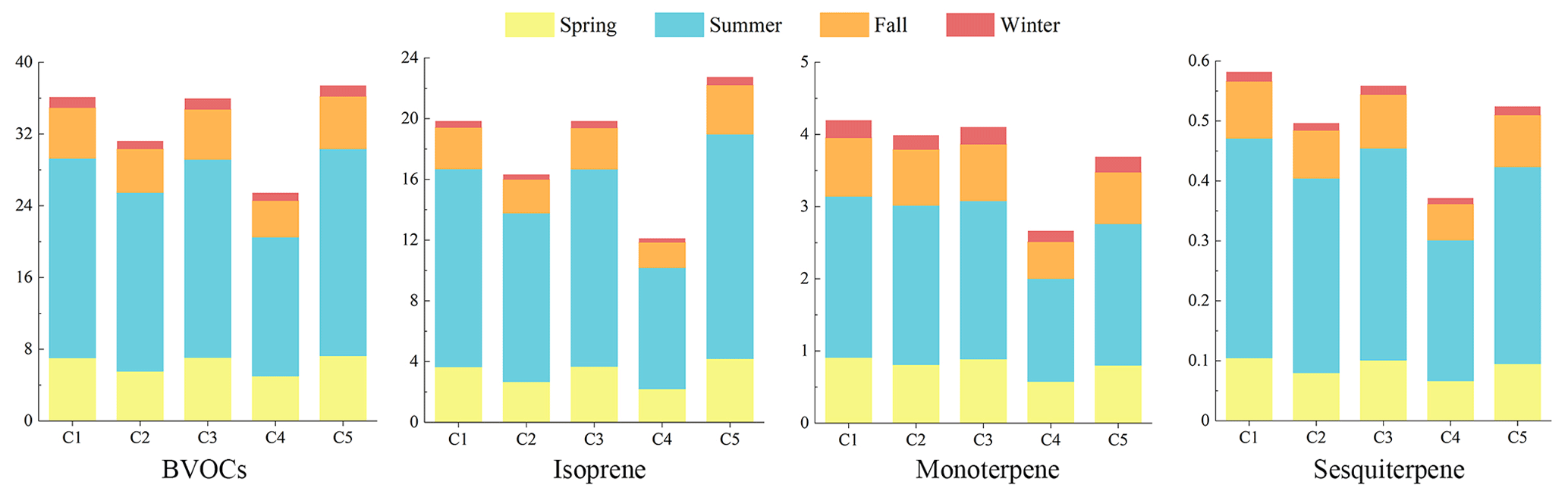
Figure 3 Seasonal emissions of isoprene, monoterpenes, sesquiterpenes, and total BVOCs of each case in China. Unit is teragrams.

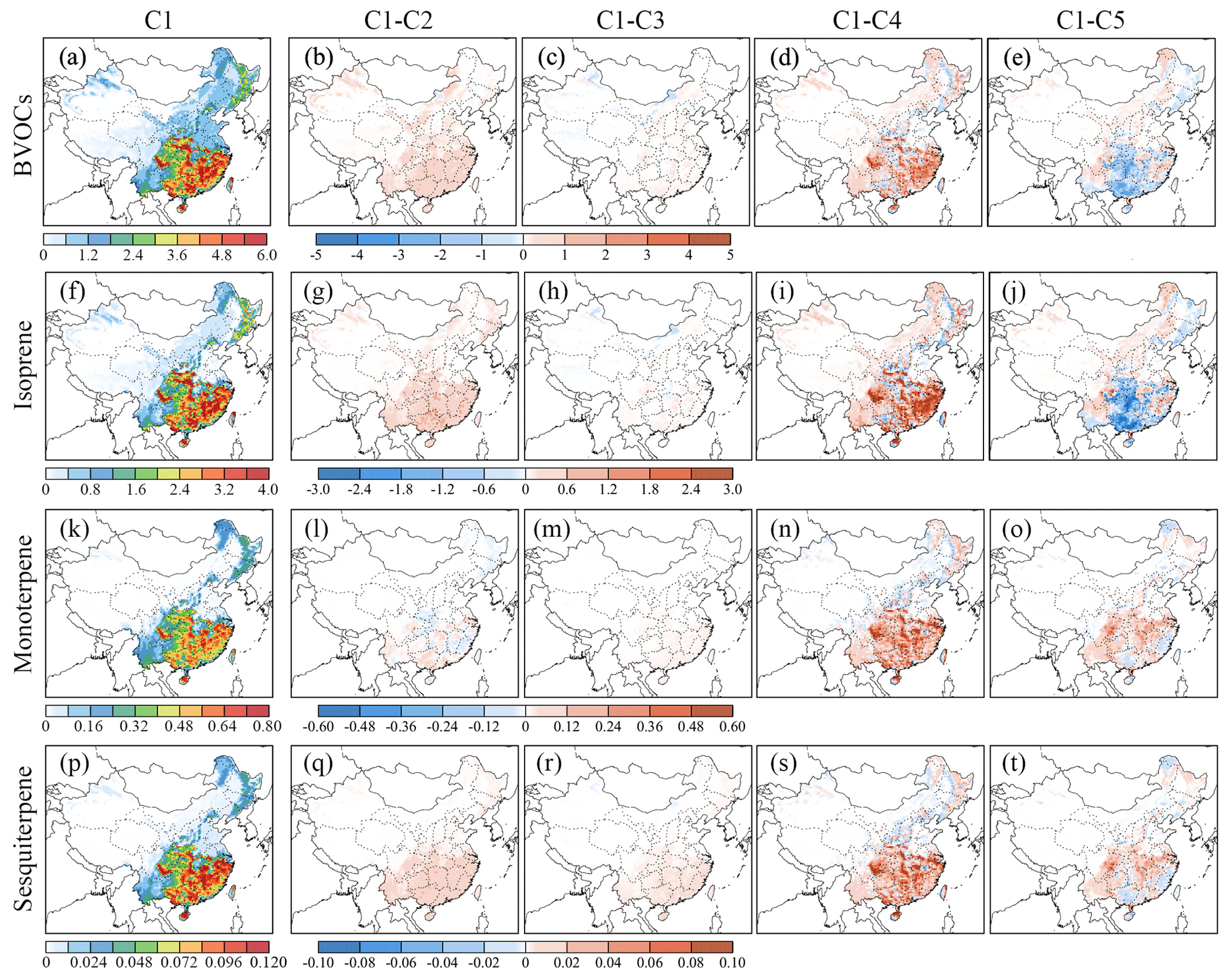
Figure 4 Comparison of three main BVOC species in different cases in summer (June, July, and August). (a, f, k, p) C1, (b, g, l, q) C1–C2, (c, h, m, r) C1–C3, (d, i, n, s) C1–C4, and (e, j, o, t) C1–C5. Unit is milligrams per square meter per hour (mg m⁻² h⁻¹).

Since a large proportion of BVOCs is released in summer, contributing about 62 % of total annual emissions, the analysis of the spatial distribution is mainly concentrated on summer BVOC emissions. Figure 4 illustrates the spatial distribution of total BVOCs, isoprene, monoterpenes, and sesquiterpenes during summer in C1 as well as the comparisons between C1 and the other cases. In general, the difference in the spatial distribution of BVOCs mainly focuses on central and southeastern China, and the differences induced by different LC products are more significant than those by different LAI products. Isoprene, monoterpene, and sesquiterpene emissions show similar distribution patterns with hotspots primarily located in central and southeastern China, as shown in Fig. 4f, k, and p. This is due to the high density of tree covers in those regions. Although GLASS has the same temporal resolution of 8 d as MOD15, differences between the two products still play an important role in impacting the BVOC emissions (Figs. 2 and 4b). According to Fig. 4a and q, the emission distribution of isoprene and sesquiterpene differs between C1 and C2, consistent with the difference in GLASS and MOD15 in summer (Fig. 2). Compared to C2 and C3, the changes in the spatial distribution of BVOC emissions in C4 and C5 are more significant. This is because the impact on BVOC emissions decreases when LAIv exceeds three (Guenther et al., 2012). Higher BVOC emissions in southern China in C1 compared to C4 are due to higher vegetation cover in C1, as shown in Fig. 4i, n, and s. C4 uses the C3S LC as the model input, with crops dominating in nearly half of China. This results in lower BVOC estimations in C4 because of the relatively low EF of the crop for BVOC emissions compared to the other PFTs (Figs. 1 and S5). The spatial distribution of isoprene emission in C5 is conspicuously different from that in C1, which is consistent with a difference in the broadleaf tree distribution (Fig. S5). Although C5 shows a higher forest cover than C1 in the north of China, the isoprene emission in C1 is higher than in C5 likely due to the difference in the grass distribution and the impact of temperature. Cooler temperatures at higher latitudes inhibit the release of isoprene from forests (Guenther et al., 2006).

3.2.3 Comparison with previous studies

Table 3 illustrates the annual BVOC emissions estimated by MEGAN in China in this study and previous studies. The annual BVOC emissions in this study range from 25.42–37.39 Tg, within the range of 17.30–54.60 Tg reported in the literature from 2001 to 2018. BVOC emissions estimated by this study are higher than 18.85 and 23.54 Tg estimated by Fu and Liao (2012) and Wu et al. (2020), respectively. However, the results of this study are lower than 58.9 Tg estimated by Li et al. (2020) for 2018. Several factors may account for the differences between this study and previous studies. One major reason could be the increase in forest coverage. According to the National Forest Resources census reports, forest coverage increased by about 18.8 % between 2003 and 2013 (SFA, 2003, 2014). In addition, BVOC emissions can be influenced by the inputs and algorithms used in the MEGAN model. In this study, the default EFs listed in Guenther et al. (2012) are used for all BVOC species. Fu and Liao (2012) used a set of EFs with 25 PFTs for isoprene and monoterpenes, which generally have lower EFs than the default ones used in MEGAN. Consequently, their study reported much lower BVOC emissions of 18.85 Tg compared to our findings. Wu et al. (2020) used the same datasets of MODIS MOD15A2H and MODIS MCD12Q1 as this study but estimated lower BVOC emissions due to lower area fractions of high-isoprene-emitting broadleaf trees (Guenther et al., 2012) and no inclusion of crop area in calculations for China. Moreover, Li et al. (2020) reported a considerable difference in BVOC emissions compared to this study, mainly due to the combined effect of emission rate and PFTs. Liu et al. (2020) produced the basal emission rates for 192 plant species and categorized them into 82 PFTs for China, resulting in more BVOC estimates. Besides, the higher estimate of 35.48 Tg for 2016 by Wang et al. (2021) may be attributed to the overestimated temperature. This is the primary reason for the significant difference between this study and theirs. In conclusion, uncertainties in the MEGAN simulations can be attributed to these factors in different years, and such uncertainties can lead to significant differences between this study and previous studies. Nonetheless, this study suggests that the simulated BVOC emissions fall within acceptable limits compared to the previous studies.

Table 3 Previous studies of BVOC emissions estimated using MEGAN in China; unit is teragrams per year.

3.3 Sensitivity of O₃ to BVOC emissions

3.3.1 Spatial distribution of O₃

Figure 5 displays the spatial distribution of MDA1 O₃ and MDA8 O₃ concentrations formed by the BVOCs during the summer in C1 as well as the difference between C1 and other cases. Changing the LC dataset in the MEGAN model has a more significant impact on O₃ concentrations compared to changing the LAI dataset. The O₃ concentration hotspots are mainly concentrated in central and eastern China, with MDA1 O₃ concentrations exceeding 12 ppb in C1. This is possibly due to the combined effect of BVOC emissions and the Asian summer monsoon. The monsoon carries oceanic air masses with low O₃ concentrations and transports O₃ from southern to central and northern China (Zhao et al., 2010; Li et al., 2018). In Fig. 5d, the spatial distribution of O₃ concentration in C4 differs from that of C1, especially in central and eastern China, where the relative difference exceeds 52 %. Although C5 has higher BVOC emissions than C1 in southern China, it has little impact on O₃ formation (Fig. 4). This may be due to the effect of O₃–NO_x–VOC sensitivity, as reported by Jin and Holloway (2015). These regions belong to NO_x-limited regions in which NO_x is limited but VOCs are abundant. Thus, the higher BVOC emissions have minimal effects on the O₃ formation. Conversely, areas with low VOC emissions, such as the NCP and YRD, will contribute more to the O₃ formation when VOC emissions increase. The spatial distribution pattern of MDA8 O₃ is similar to that of MDA1 O₃ in C1, but its concentration is 3–6 ppb lower than that of MDA1 O₃.

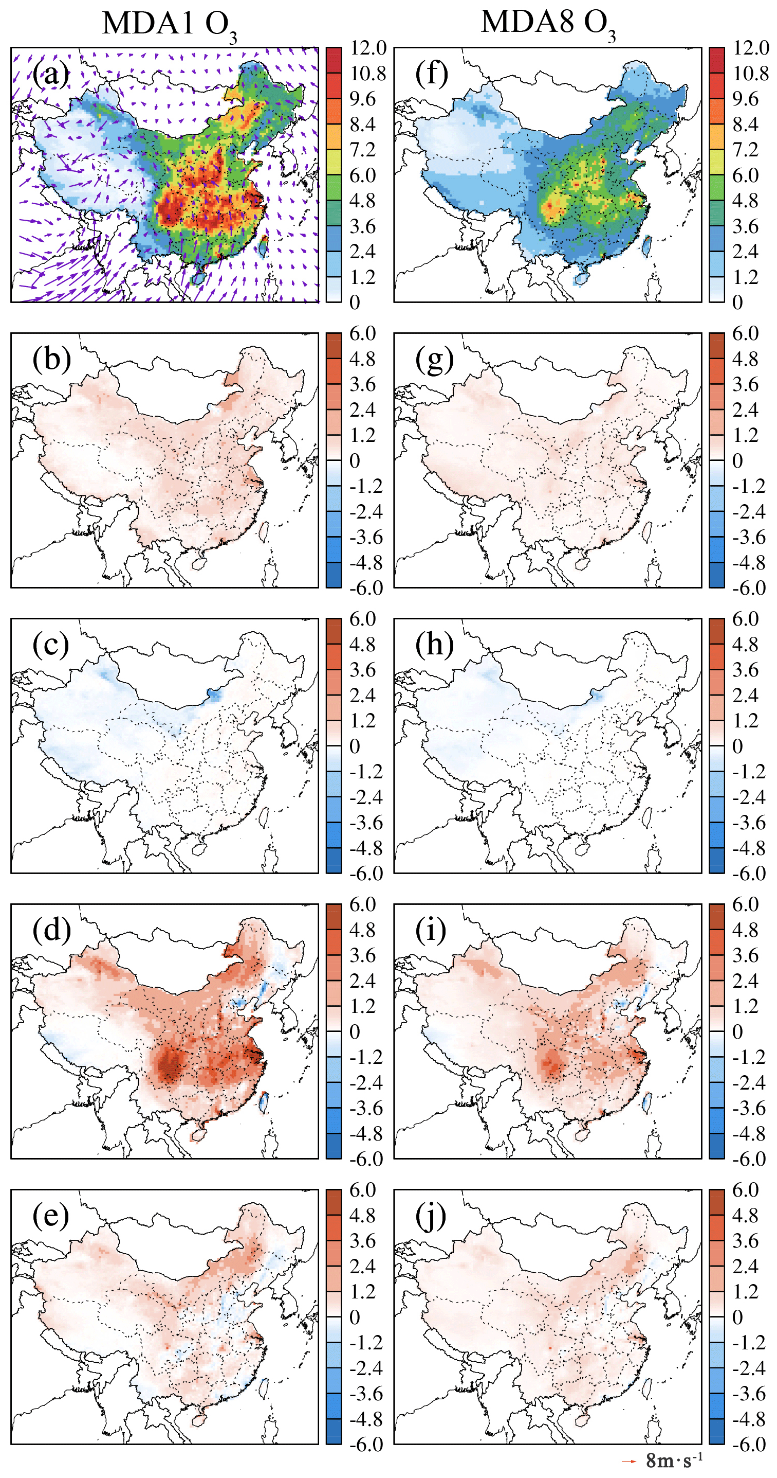
Figure 5 Spatial distributions of MDA1 O₃ and MDA8 O₃ from biogenic sources in the different cases in summer. (a, f) C1, (b, g) C1–C2, (c, h) C1–C3, (d, i) C1–C4, and (e, j) C1–C5. Unit is parts per billion.

3.3.2 Temporal distribution of O₃

Figure 6 illustrates the contribution of BVOC emissions to MDA1 O₃ and MDA8 O₃ in China and important regions in different seasons. O₃ concentrations, which are formed by BVOCs, show seasonal variations in China, with the highest in summer and the lowest in winter. This is a result of the interplay between BVOC emissions and wind. In the PRD, wind plays an important role in O₃ concentrations (Fig. S6), as it can transport clean oceanic air masses to the southeast of China, decreasing local O₃ concentrations (Zhao et al., 2010). However, wind transports heavy pollutants from northern to southern China in the fall, increasing O₃ concentrations in the PRD (Li et al., 2018). In addition, compared to other regions, the temperature variation in the PRD is not significant (Table S7). Therefore, the seasonal variations in O₃ are not significant in the PRD due to the combined effect of wind and temperature. The seasonal variation in O₃ formed by BVOCs also varies in different cases. In China, MDA1 O₃ concentrations increase by approximately 40 %–50 % in summer compared to spring, whereas C2 increases by 75 %. C2 also shows the highest increase in O₃ concentrations in important regions from spring to summer. Moreover, in the YRD, MDA1 O₃ in C1 is 78 % higher than in C4 because of the O₃–NO_x–VOC sensitivity, with higher BVOC emissions in VOC-limited areas leading to higher O₃ formation (Jin and Holloway, 2015). In China and other important regions, MDA8 O₃ shows a temporal distribution similar to MDA1 O₃ in all cases. However, the contribution of MDA8 O₃ to the fall season is lower than its contribution to the spring season, which contrasts with MDA1 O₃.

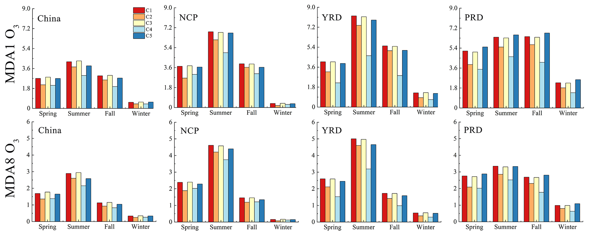
Figure 6 Seasonal-averaged concentrations of MDA1 O₃ and MDA8 O₃ from biogenic emissions in important regions and China.

3.4 Sensitivity of SOA to BVOC emissions

3.4.1 Spatial distribution of SOA and components

Figure 7 presents the spatial distribution of BSOA during summer in C1 and the difference between C1 and other cases. Changing the LC dataset in the MEGAN model has a more significant impact on BSOA formation than changing the LAI dataset. The hotspots of BSOA are mainly concentrated in central and eastern China, with the Sichuan Basin (Fig. S1) having the highest BSOA concentration of up to 9.8 µg m⁻³. This is because high surface winds transport BSOA from southern China to central China, where low wind speeds and the topography of the Sichuan Basin hinder pollutant diffusion, leading to BSOA accumulation (J. Li et al., 2017). The difference in BSOA concentrations between C1 and C2 is minor due to the slight change in BVOCs. In contrast, the difference in BSOA concentrations between C1 and C4 is significant due to the use of different LC datasets. As shown in Fig. 7d, the difference in BSOA concentrations between C1 and C4 is noticeable, especially in central and eastern China, where the relative difference is over 140 % in summer. The differences in the spatial distribution of BSOA between C1 and C5 are similar to those in isoprene, suggesting that BSOA concentrations are more sensitive to isoprene emissions. Considering the share of BSOA in the total SOA concentration in summer, the difference in BVOC emissions due to changing the MEGAN inputs can significantly impact SOA concentrations estimated by CMAQ.

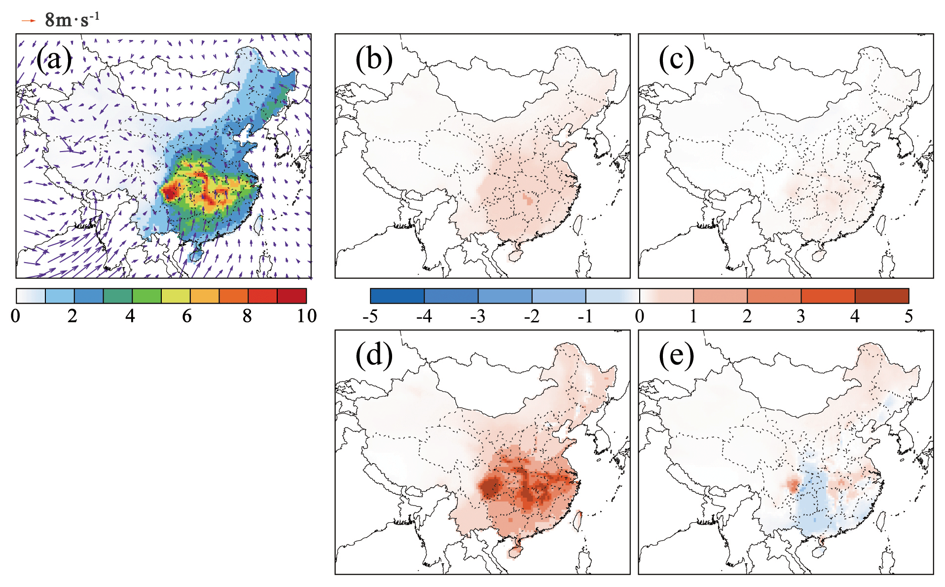
Figure 7 Spatial distributions of simulated SOA from biogenic sources in the different cases in summer. Unit is micrograms per cubic meter of air. (a) C1, (b) C1–C2, (c) C1–C3, (d) C1–C4, and (e) C1–C5.

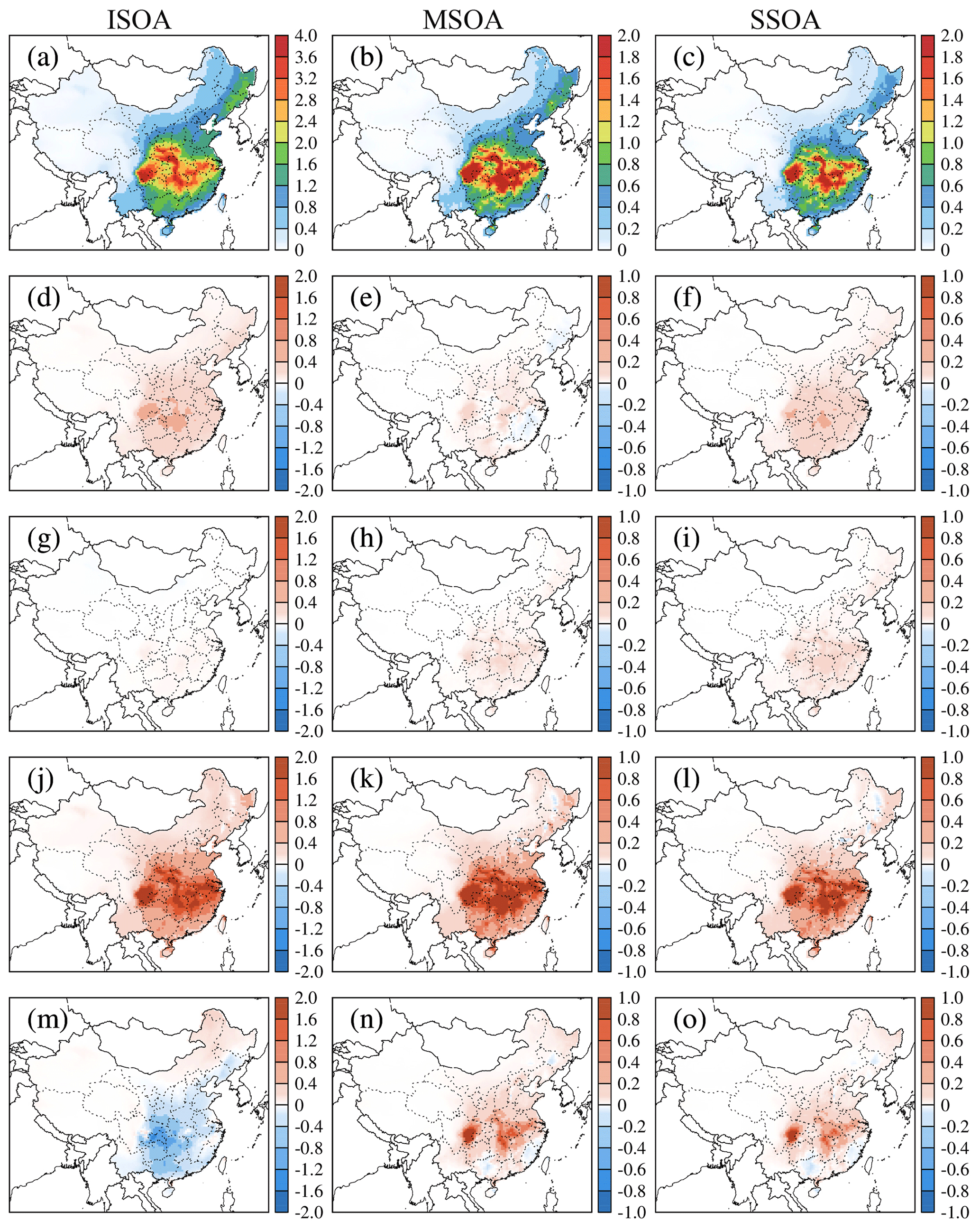
Figure 8 Spatial distributions of simulated SOA from isoprene (ISOA), monoterpenes (MSOA), and sesquiterpenes (SSOA) in the different cases in summer. (a–c) C1, (d–f) C1–C2, (g–i) C1–C3, (j–l) C1–C4, and (m–o) C1–C5). Unit is micrograms per cubic meter of air.

Figure 8 displays the spatial distribution of SOA formed by isoprene (ISOA), monoterpenes (MSOA), and sesquiterpenes (SSOA) during summer in C1 as well as the difference between C1 and the other cases. The ISOA, MSOA, and SSOA show a similar spatial distribution in China. According to Fig. 8a, b, and c, high SOA concentrations from these three BVOC species are mainly concentrated in central and eastern China. This phenomenon is likely due to the combined effect of BVOC emissions and meteorological conditions in these areas. A large amount of SOA is generated in southern China and then transported to central and eastern China due to wind effects in summer. The ISOA is the most crucial contributor to BSOA, which is 1 time higher than MSOA and 1.5 times higher than SSOA. Comparing C1 with other cases, the difference in ISOA concentrations basically shows a certain correlation with the difference in BVOCs (Fig. 4). The relative difference in ISOA concentrations between C1 and C4 can reach 160 % in eastern China, which is higher than that in MSOA and SSOA. This can be attributed to the large discrepancy in their isoprene emission (Fig. 8j, k, and l). ISOA concentrations in southeastern China are lower in C1 than in C5, but MSOA and SSOA concentrations are higher than in C5, which is due to the difference in BVOC estimations. Changing the MEGAN inputs has a large impact on isoprene emissions, which are the main contributor to BVOC emissions. This further impacts the formation of SOA.

3.4.2 Temporal distribution of SOA

Figure 9 illustrates the seasonal variation in BSOA concentrations in China and the important regions for all cases. In general, the differences in BSOA concentrations between each case are more significant in summer than in other seasons. The BSOA concentration follows the seasonal cycle of summer > spring > fall > winter in China, NCP, and YRD. However, the higher BSOA concentration in the PRD occurs during spring, and this can be attributed to changes in wind direction, from erratic winds in spring to southerly winds in summer, as shown in Fig. S7. BSOA concentrations vary slightly between C1, C3, and C5 in China, but the differences are significant between C2 and C4, particularly in the YRD, where the summer BSOA in C1 is 2.5 times higher than in C4. This is because the summer BVOC emissions in C1 are higher than those in C4 in the YRD (Fig. S8) and thus formed more BSOA. C1 tends to have higher BSOA concentrations than C5 in most regions of China. However, this differs in the PRD, where C5 has higher BSOA concentrations due to higher isoprene emissions (Fig. 4).

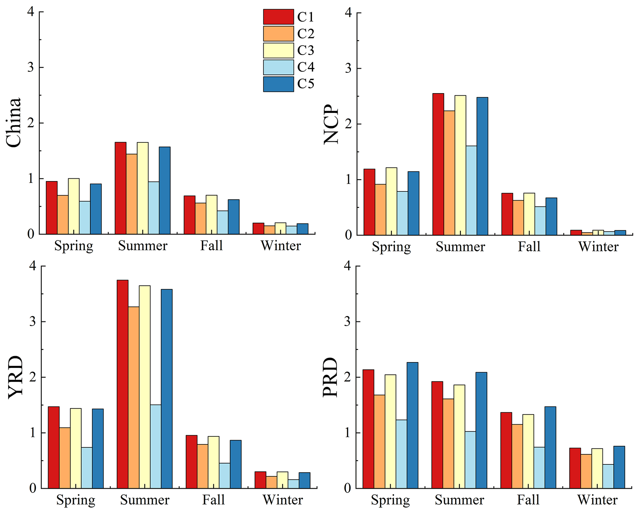
Figure 9 Seasonal distributions of biogenic SOA (BSOA) for all cases in important regions and China. Unit is micrograms per cubic meter of air.

4 Conclusion

In this study, we used the different LAI and LC datasets as the MEGAN inputs to estimate the BVOC emissions in 2016 over China and then utilized the WRF-CMAQ model to quantify the contribution of BVOCs to O₃ and SOA concentrations. Besides, the impact induced by those inputs on O₃ and SOA formation was also evaluated. Five experiments were conducted based on three LAI satellite products (GLASS, MOD15, and CGLS) and three LC satellite products (MCD12Q1, C3S, and CGLS). According to model validations, C4 with GLASS and C3S LC was a better choice for China BVOC estimations than other scenarios. BVOC emissions in China ranged from 25.42 to 37.39 Tg in 2016 and were mainly concentrated in central and southeastern China due to the high density of tree covers in those regions. In comparison with LAI inputs, using different LC satellite products had a more significant impact on BVOC emissions.

The O₃ formed by BVOCs was mainly concentrated in central and eastern China, where O₃ concentrations could reach 12 ppb. This was likely due to the combined effect of BVOC emissions and the summer monsoon. According to the sensitivity analysis, C1 contributed the most to the summer O₃, which was 78 % higher than C4 in the YRD. The BSOA was also concentrated in central and eastern China, especially in the Sichuan Basin, where the BSOA concentration was up to 9.8 µg m⁻³. The differences in BSOA concentrations between C1 and C2 are inconspicuous due to the slight change in BVOCs induced by LAI inputs. In contrast, the LC inputs show higher impacts on BSOA concentrations. This is the same as for O₃. Therefore, changing LAI and LC datasets in the model impacts O₃ and SOA formation, where the LC shows a more pronounced effect than the LAI. Our results suggest that the uncertainties in MEGAN inputs should be carefully considered in future O₃ and SOA simulations.

From 2000 to 2017, the global leaf area of vegetation increased by 6.6 % due to direct land use management, which may also enhance BVOC emissions and further affect air quality. Thus, the findings of this study can be extended to other regions and global scales, suggesting an urgent need to construct a reliable BVOC emission inventory for local and global scales and to evaluate their impacts on air quality. However, the limitation in observed data of BVOCs and organic components impedes the construction of an accurate emission inventory. Therefore, field measurements are needed to provide more data for model validations. In addition, urban BVOC emissions play important roles in urban air quality. It would be interesting to study the impact of biogenic sources on urban air quality using high-resolution LC satellite maps.