Dependency of vertical velocity variance on meteorological conditions in the convective boundary layer

Measurements of vertical velocity from vertically pointing Doppler lidars are used to derive the profiles of normalized vertical velocity variance. Observations were taken during the FESSTVaL (Field Experiment on Submesoscale Spatio-Temporal Variability in Lindenberg) campaign during the warm seasons of 2020 and 2021. Normalized by the square of the convective velocity scale, the average vertical velocity variance profile follows the universal profile of Lenschow et al. (1980). However, daily profiles still show a high day-to-day variability. We found that moisture transport and the content of moisture in the boundary layer could explain the remaining variability of the normalized vertical velocity variance. The magnitude of the normalized vertical velocity variance is highest on clear-sky days and decreases as the absolute humidity increases and surface latent heat flux decreases on cloud-topped days. This suggests that moisture content and moisture transport are limiting factors for the intensity of turbulence in the convective boundary layer. We also found that the intensity of turbulence decreases with an increase in the boundary layer cloud fraction during FESSTVaL, while the latent heating in the cloud layer was not a relevant source of turbulence in this case. We conclude that a new vertical velocity scale has to be defined that would take into account the moist processes in the convective boundary layer.

1 Introduction

Turbulence has an important role in distributing heat, momentum, moisture and trace gases from the land surface to the free troposphere. As a measure of the intensity of turbulent structures in a convective boundary layer, such as updrafts or thermals, the vertical velocity variance, ${\mathit{\sigma }}_w^{\mathrm{2}}$, is frequently used. The vertical velocity variance normalized by the square of the convective velocity scale (Deardorff, 1970), ${\mathit{\sigma }}_w^{\mathrm{2}}/w_{*}^{\mathrm{2}}$, has been studied using both observational data (e.g. Hogan et al., 2009; Maurer et al., 2016) and numerical models (e.g. Lenschow et al., 2012; Zhou et al., 2019). Previous studies consistently show that the mean vertical profile of ${\mathit{\sigma }}_w^{\mathrm{2}}/w_{*}^{\mathrm{2}}$ follows the universal function introduced by Lenschow et al. (1980):

$$\begin{array}{}\text{(1)}& {\mathit{\sigma }}_w^{\mathrm{2}}/w_{*}^{\mathrm{2}}=\mathrm{1.8}(z/z_i{)}^{\mathrm{2}/\mathrm{3}}{\left(\mathrm{1}-\mathrm{0.8}(z/z_i)\right)}^{\mathrm{2}},\end{array}$$

where z represents the height above ground level and z_i is the depth of the mixed layer. This function gives an asymmetric vertical profile with a maximum of ${\mathit{\sigma }}_w^{\mathrm{2}}/w_{*}^{\mathrm{2}}$ at about 0.3 z_i–0.4 z_i. The universal profile was derived from in situ aircraft measurement data recorded during AMTEX (Air Mass Transformation Experiment) that took place over the East China Sea during wintertime cold-air outbreaks.

Although there is universality in the mean ${\mathit{\sigma }}_w^{\mathrm{2}}/w_{*}^{\mathrm{2}}$ profile across many case studies and seasons in both clear-sky and cloud-topped boundary layers, the variability of daily profiles of ${\mathit{\sigma }}_w^{\mathrm{2}}/w_{*}^{\mathrm{2}}$ is high, and their dependency on the boundary layer conditions varies from case to case. A considerable scatter of the ${\mathit{\sigma }}_w^{\mathrm{2}}/w_{*}^{\mathrm{2}}$ profiles was found in the study of Hogan et al. (2009), which analysed profiles of 2 clear-sky days and 4 shallow-cumulus days. They found that the mean profile was similar to the universal profile of Lenschow et al. (1980) with no significant difference between the profiles on clear-sky and cloud-topped days. Lareau et al. (2018) conducted a study at the ARM Southern Great Plains (SGP) site in Oklahoma, United States, and found significantly different behaviour of ${\mathit{\sigma }}_w^{\mathrm{2}}/w_{*}^{\mathrm{2}}$ compared to the previous study of Chandra et al. (2010) conducted at the same location. A higher magnitude of ${\mathit{\sigma }}_w^{\mathrm{2}}/w_{*}^{\mathrm{2}}$ was found on days with a higher cloud fraction in Chandra et al. (2010), while Lareau et al. (2018) found the highest magnitude of ${\mathit{\sigma }}_w^{\mathrm{2}}/w_{*}^{\mathrm{2}}$ at an intermediate range of cloud fraction. Moreover, Lareau et al. (2018) observed a lower magnitude of ${\mathit{\sigma }}_w^{\mathrm{2}}/w_{*}^{\mathrm{2}}$ on clear-sky days compared to the cloud-topped days, opposite to Chandra et al. (2010), who found the largest magnitude of ${\mathit{\sigma }}_w^{\mathrm{2}}/w_{*}^{\mathrm{2}}$ in the clear-sky category. In a year-long dataset from the same site (ARM SGP), Berg et al. (2017) found a sensitivity of the ${\mathit{\sigma }}_w^{\mathrm{2}}/w_{*}^{\mathrm{2}}$ magnitude on clear-sky days to the season, friction velocity, stability and wind shear across the boundary layer top. An earlier study of Lenschow et al. (2012) also found a considerable residual scatter after normalization in the daily profiles of the ${\mathit{\sigma }}_w^{\mathrm{2}}/w_{*}^{\mathrm{2}}$, with about 10 % of the variations that could not be explained by the effects of wind shear, stability or variability in land surface properties. Furthermore, during the days with mesoscale circulations, such as longitudinal roll circulations, the peak of the ${\mathit{\sigma }}_w^{\mathrm{2}}/w_{*}^{\mathrm{2}}$ profile was lifted to about 0.6 z_i–0.7 z_i even when the surface heat flux values remained comparable to the other cases (Lenschow et al., 2012).

The following research questions stem from the previous studies: where does the residual variation in the daily profiles after normalization come from? Is cloud fraction a relevant parameter to study the changes in the magnitude of ${\mathit{\sigma }}_w^{\mathrm{2}}/w_{*}^{\mathrm{2}}$ from case to case? Are boundary layer clouds a significant source of turbulence in the convective boundary layer?

Various observational methods can be used to obtain the variance of vertical velocity measurements. In the cited studies, most of the vertical velocity data were obtained by in situ aircraft measurement, but the measurements were limited to the height and the number of flights. The conventional meteorological tower using sonic anemometers can be used to obtain the vertical velocity variance (e.g. Bonin et al., 2016). However, in this case, the height of the retrieval is also limited depending on the height of the tower. These limitations of the earlier measurement techniques are overcome by the advance of ground-based remote sensing using Doppler lidars. Doppler lidars are able to measure continuously and can cover the entire boundary layer depth. Besides vertical velocity measurement, Doppler lidars have been used to measure wind speed and wind direction (e.g. Päschke et al., 2015), wind gusts (e.g. Suomi et al., 2017), and turbulence (e.g. Sathe et al., 2015; Smalikho and Banakh, 2017) and to identify coherent structures (e.g. Ansmann et al., 2010; Cheliotis et al., 2020). Doppler lidars are a reliable method to retrieve the ${\mathit{\sigma }}_w^{\mathrm{2}}/w_{*}^{\mathrm{2}}$ profile, as shown in a comparison between the ${\mathit{\sigma }}_w^{\mathrm{2}}/w_{*}^{\mathrm{2}}$ profile derived from a Doppler lidar, large eddy simulations (LESs) and the empirical profile (Lenschow et al., 2012).

In this study, we investigate the dependency of ${\mathit{\sigma }}_w^{\mathrm{2}}/w_{*}^{\mathrm{2}}$ on the meteorological parameters using Doppler lidar measurements. The aim is to find the key parameters that explain the day-to-day variability of ${\mathit{\sigma }}_w^{\mathrm{2}}/w_{*}^{\mathrm{2}}$ that could be used in the future to derive a scaling velocity taking into account the missing factors controlling the intensity of turbulence in the convective boundary layer. The Doppler lidar data were collected during two consecutive summer periods of the FESSTVaL (Field Experiment on Submesoscale Spatio-Temporal Variability in Lindenberg) campaign (https://fesstval.de/, last access: 25 July 2022), from June–August 2020 and May–August 2021. The measurement campaigns aimed at identifying sub-mesoscale variability, such as atmospheric boundary layer structure, cold pools and wind gusts, and took place at the Meteorological Observatory Lindenberg – Richard Aßmann Observatory (MOL-RAO) of the German Weather Service (DWD) near Berlin. The structure of this paper is as follows: we describe the instruments and the measurements in Sect. 2. The selected days and case categories are described in Sect. 3. In Sects. 4 and 5, we present the results and a discussion, followed by the conclusion at the end of the paper.

2 Data, method and measurements

Two different units of the Halo Photonics StreamLine XR Doppler lidar set up in a vertical stare configuration were used to measure the vertical velocity during FESSTVaL. In the 2020 measurement campaign, the Halo Photonics StreamLine XR 161 (DL161) was used, while in the 2021 measurement campaign, we used the Halo Photonics StreamLine XR 146 (DL146). The details of the specifications are shown in Table 1. Besides the Doppler lidar data, the routine measurements from the Falkenberg site are used in this study. The surface heat flux for the calculation of the convective velocity scale was obtained from the eddy-covariance measurement using a sonic anemometer (USA-1, METEK GmbH) and an infrared gas analyser (LI7500RS, Licor Inc.) at a height of 2.4 m. We also used the friction velocity (u_*) retrieved from the same instrument for the analysis in Sect. 4. The 10 m wind speed, relative humidity at 10 and 98 m, and temperature at 98 m were obtained from the 99 m meteorological mast which is located near the Doppler lidar position as shown in Fig. 1 using a Thies cup anemometer and a Vaisala HMP-45. In addition, precipitation measurements were used to sort out the rainy days in the collected datasets and the ceilometer data from the CHM15k-080066 instrument to make a comparison to the cloud detection from Doppler lidar data.

Table 1 Technical specification of Doppler lidars DL161 and DL146.

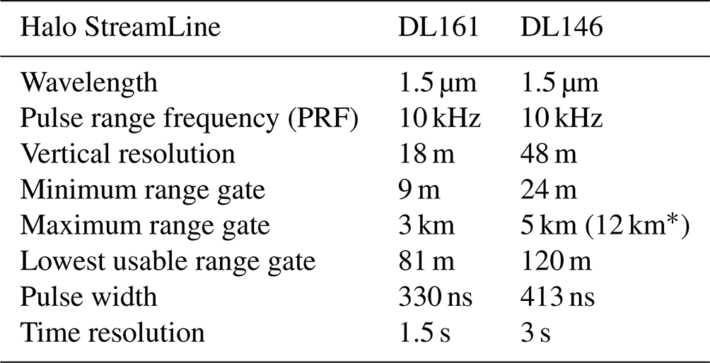
^∗ Period after 12 August 2021.

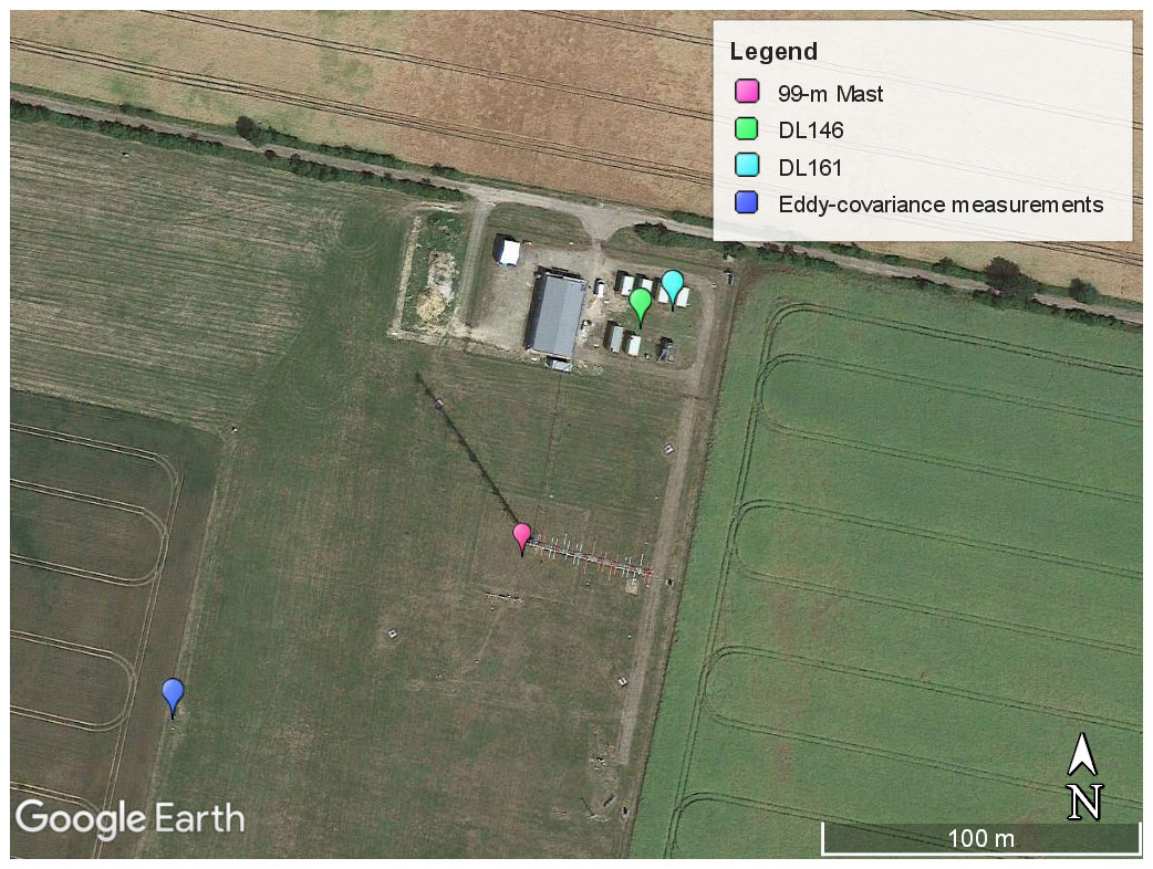
Figure 1 Measurement location in Falkenberg, MOL-RAO (source: © Google Earth).

For Doppler lidar data quality control, different signal-to-noise ratio (SNR) filters were applied to the two datasets. For DL161 data, we applied 1.005 as a threshold of the backscatter intensity (SNR+1) parameter in the first filtering step. The following additional procedure was applied to the DL161 data after the SNR filtering. The tested data point is removed if the difference between the tested data to the surrounding data in an 8 × 8 matrix is more than 5 m s⁻¹, while for the DL146 data, the SNR+1 threshold is different from day to day in order to obtain more data at the highest height level. A threshold within a range between 0.994 and 1.005 is determined as a limit close to the data which is no longer distributed over the search band (±19 m s⁻¹) as shown in Fig. 2. Besides the SNR filter, the first two elevation levels in DL146 and first four elevation levels in DL161 datasets were removed due to the high noise level in these lowest range gates as shown by the horizontal straight line in Fig. 2. Therefore, the lowest level is 81 m for DL161 and 120 m for DL146. To ensure comparability between the two different Doppler lidar units, an intercomparison between DL161 and DL146 was performed on 23–25 July 2021 in vertical stare mode. The 1 min averages of vertical velocity at a height of 120 m show a good agreement between the two Doppler lidars (Fig. 3e). Furthermore, we compared the mixed-layer depth and convective velocity between the two Doppler lidars within the analysis time window between 10:00–15:00 UTC, except for 25 July 2021, for which we only used the time window up to 14:30 UTC due to the rain events in the afternoon. Although the mixed-layer height has a small bias, the comparison results in Fig. 3 show a good agreement in both parameters with a coefficient correlation of 0.99 for mixing layer depth and the convective velocity.

Figure 2 A 2D histogram of intensity (SNR+1) and vertical velocity on 24 July 2021 from DL161 (a) and DL146 (b). The dashed red line indicates the 1.005 of SNR+1, and the horizontal straight blue line at 15 m s⁻¹ is the example of noise data in the lowest range gates.

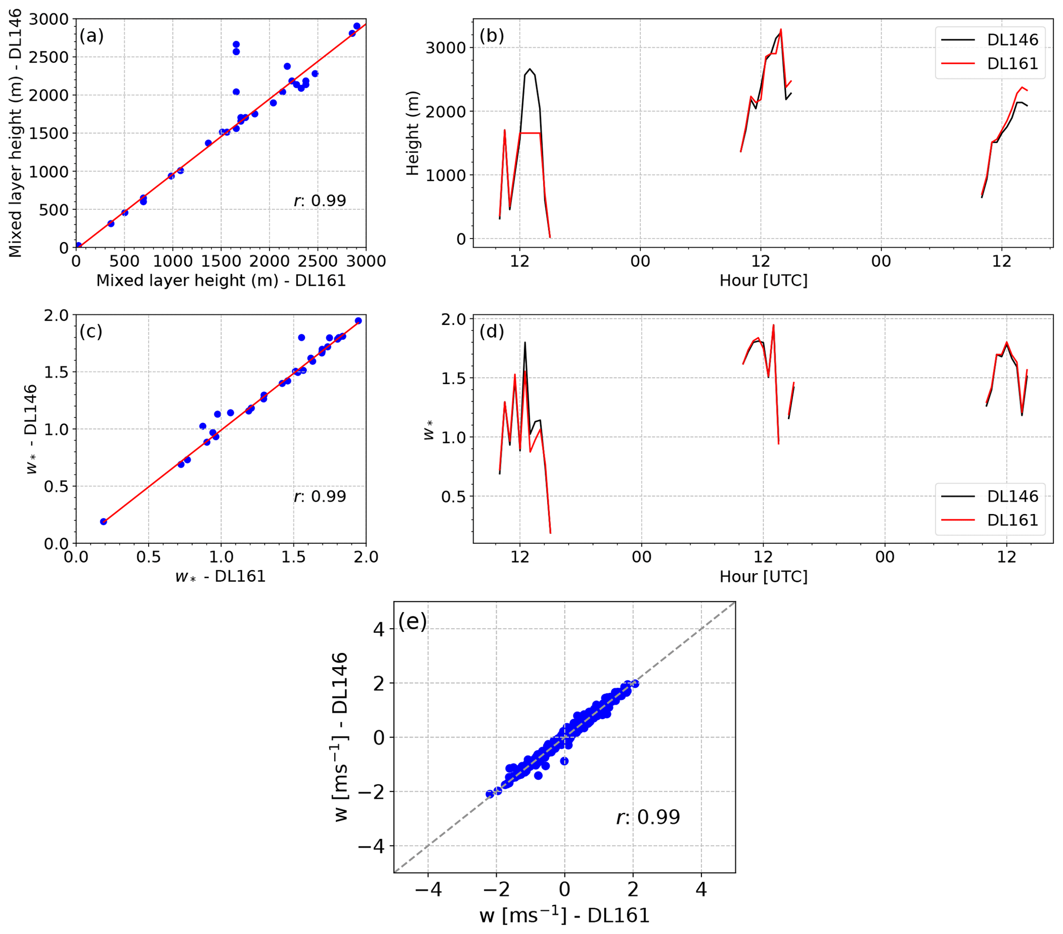
Figure 3 Comparison between the two co-located Doppler lidars, DL161 and DL146, during 23, 24 and 25 July 2021 within the time window 10:00–15:00 UTC, except for 25 July only up to 14:30 UTC on (a, b) mixed-layer height, (c, d) convective velocity scale and (e) 1 min average of vertical velocity comparison at 120 m.

The vertical velocity variance was calculated for 30 min periods using the method from Lenschow et al. (2000) to remove uncorrelated noise in the higher-order statistics. First, auto-covariance is calculated for the first 40 points. Next, the corrected variance was estimated by extrapolating the autocovariance to zero lag by linear extrapolation. The difference between the extrapolated variance at zero lag and the uncorrected variance is the uncorrelated noise.

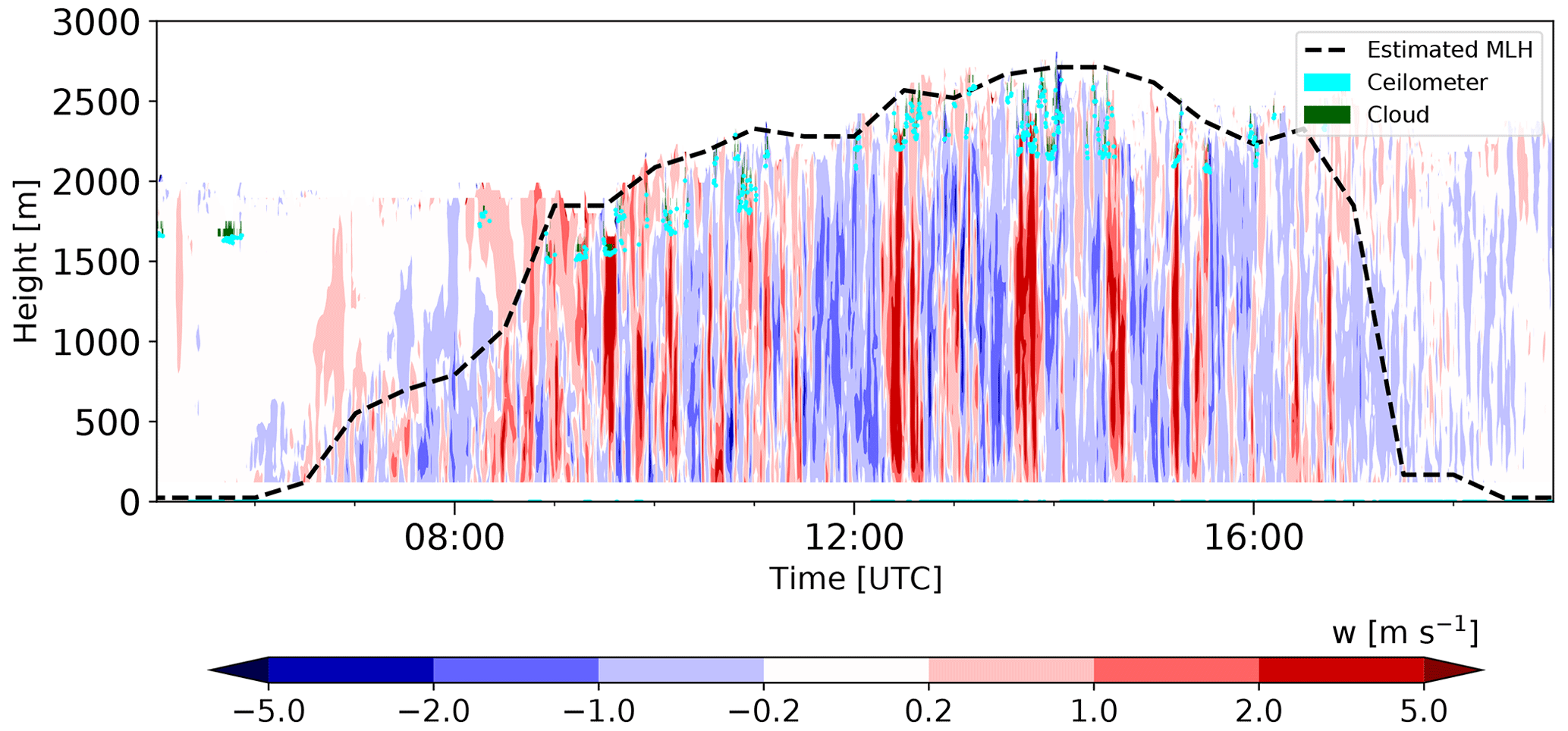
Figure 4 Vertical velocity averaged over 1 min on 11 June 2021. The dashed black line indicates the estimated mixing-layer height based on the Doppler lidar measurements, the green dot shows the clouds from attenuated backscatter coefficient from the Doppler lidar, and the cyan dot indicates the cloud base height based on ceilometer measurements.

For the analysis, the vertical velocity variance was normalized by the convective velocity as shown in Eq. (2). The equation is derived from Eq. (2.80) in Garratt (1994).

$$\begin{array}{}\text{(2)}& w_{*}={\left[g{z}_i(\mathrm{SHF}+\mathrm{0.07}\mathrm{LHF})/\left(T_{\mathrm{v}}\mathit{\rho }{c}_p\right)\right]}^{\mathrm{1}/\mathrm{3}},\end{array}$$

where g is the acceleration of gravity, z_i is the estimated mixing-layer height, SHF and LHF are the surface sensible and latent heat fluxes respectively, c_p is the specific heat capacity, T_v is the virtual temperature, and ρ is the air density. Besides the normalization of vertical velocity variance, the height also has to be normalized by the mixing-layer height. The latter was estimated using the variance method with a 0.09 threshold in both datasets. The mixed-layer top is estimated as the first layer for which the variance is below the threshold. An example of the estimated mixing-layer height is shown in Fig. 4 by the dashed black line. We also used cloud fraction as one of the meteorological parameters for the analysis. Clouds are detected using the attenuated backscatter from the Doppler lidar data, employing a threshold of 10⁻⁴ m⁻¹ sr⁻¹. The clouds identified based on the Doppler lidar data (green) and ceilometer data (cyan) show good agreement (Fig. 4).

3 Data selection and categorization

Two main categories were created based on the presence of clouds: clear-sky and cloud-topped days. The days with rainy events during the day are excluded from the cloud-topped category and put into the rainy day category. The analysis used a total of 88 selected days from two consecutive summer periods, consisting of 11 clear-sky days, 59 cloud-topped days and 18 rainy days. Specifically for rainy days, the rain period was excluded. An example of 1 min average vertical velocity and 30 min average of the vertical velocity variance for a clear-sky, cloud-topped and rainy day is given in Fig. 5. We focus on the clear-sky and cloud-topped days for the analysis in this study. The impact of rainy events on the atmospheric boundary layer turbulence is not the focus of our study and would require a separate investigation. However, we keep the mean profile of ${\mathit{\sigma }}_w^{\mathrm{2}}/w_{*}^{\mathrm{2}}$ on the rainy days for comparison purposes in this study.

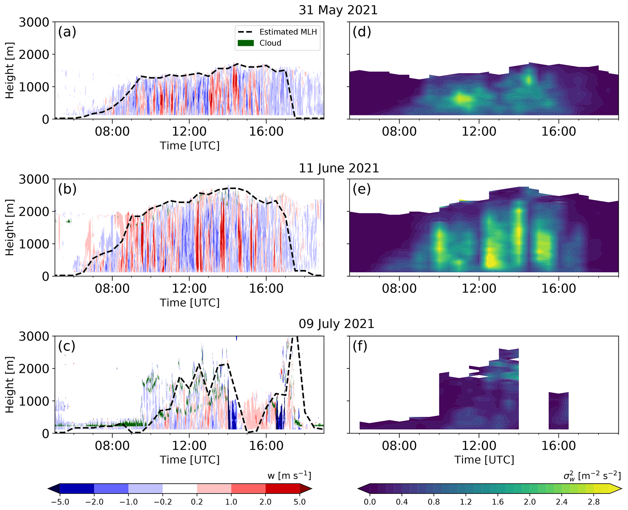
Figure 5 Example of (a–c) 1 min averages of vertical velocity and (d–f) 30 min averages of variance of vertical velocity on a clear-sky day (31 May 2021), cloud-topped day (11 June 2021) and rainy day (9 July 2021). The estimated mixing-layer height based on the Doppler lidar measurements is indicated by a dashed black line, while the cloud layer is given in green.

The hourly cloud fraction is used to categorize clear-sky and cloud-topped days. Days with an average cloud fraction above 0.003 within the analysis period were categorized as cloud-topped. This study considers the low clouds but does not consider the type of clouds and focuses more on finding a general dependency of the ${\mathit{\sigma }}_w^{\mathrm{2}}/w_{*}^{\mathrm{2}}$ profile on cloud fraction.

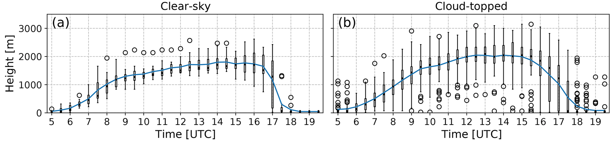
Figure 6 Composite of 30 min mixing-layer height for (a) clear-sky days and (b) cloud-topped days. The blue line indicates the mean of mixing-layer height, the box denotes the upper quartile and lower quartile, and the whiskers show the extension of 1.5 times the interquartile range. The outliers are denoted by the circles.

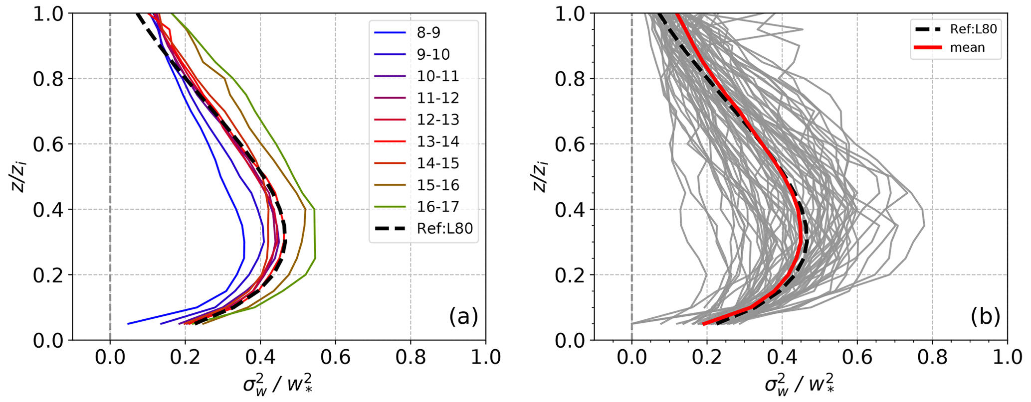
Figure 7 (a) Diurnal change of the composite hourly profiles of ${\mathit{\sigma }}_w^{\mathrm{2}}/w_{*}^{\mathrm{2}}$ from clear-sky and cloud-topped days combined and (b) daily profiles of ${\mathit{\sigma }}_w^{\mathrm{2}}/w_{*}^{\mathrm{2}}$ showing individual days (grey line) and the mean profile (red line). The universal profile of Lenschow et al. (1980) is given as a dashed black line.

All of the analysis in this study is based on the time period from 10:00 to 15:00 UTC with the assumption that the boundary layer is in a relatively well developed stage during this period. Figure 6 shows the evolution of the mixing-layer height on clear-sky days and cloud-topped days from the 30 min composites in each case. A higher boundary layer height is observed on cloud-topped days compared to clear-sky days. The composite of the hourly ${\mathit{\sigma }}_w^{\mathrm{2}}/w_{*}^{\mathrm{2}}$ profiles from combined clear-sky and cloud-topped days is shown in Fig. 7a. The magnitude of the ${\mathit{\sigma }}_w^{\mathrm{2}}/w_{*}^{\mathrm{2}}$ profiles increases from the morning hours as the boundary layer starts to develop till about 10:00 UTC. During the day when the boundary layer was well developed, between 10:00 and 15:00 UTC, the magnitude of the ${\mathit{\sigma }}_w^{\mathrm{2}}/w_{*}^{\mathrm{2}}$ profile becomes less variable. After 15:00 UTC, the magnitude of the ${\mathit{\sigma }}_w^{\mathrm{2}}/w_{*}^{\mathrm{2}}$ profile increases again as the surface heat flux decreases, and the boundary layer starts to collapse in the afternoon hours.

4 Results

4.1 Vertical velocity variance

The mean ${\mathit{\sigma }}_w^{\mathrm{2}}/w_{*}^{\mathrm{2}}$ profile from the selected clear-sky and cloud-topped days is similar to the empirical universal profile as shown in Fig. 7b. However, as in the previous studies, there is considerable variation in the day-to-day ${\mathit{\sigma }}_w^{\mathrm{2}}/w_{*}^{\mathrm{2}}$ profiles. This variability remains after scaling the vertical velocity variance with $w_{*}^{\mathrm{2}}$, which signifies that there is another relevant factor that controls the intensity of turbulence in the convective boundary layer, other than the generation of turbulence by buoyancy, that is not accounted for. Furthermore, we also tested the effect of including shear in the scaling velocity, introduced by Moeng and Sullivan (1994), and found no significant reduction in the variability of the day-to-day ${\mathit{\sigma }}_w^{\mathrm{2}}/w_{*}^{\mathrm{2}}$ profiles (not shown).

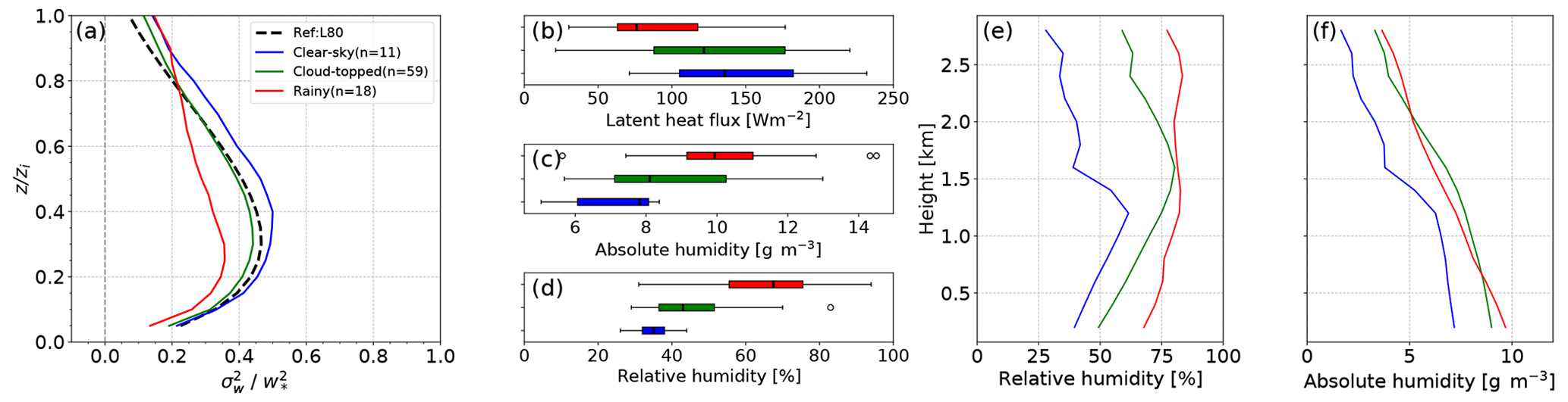
Figure 8 (a) Average profiles of ${\mathit{\sigma }}_w^{\mathrm{2}}/w_{*}^{\mathrm{2}}$ of the three main categories: clear-sky, cloud-topped and rainy days. The universal profile is given as a dashed black line. Box plot of the (b) surface latent heat flux (LHF), (c) absolute humidity and (d) relative humidity (RH) averaged over the three categories and (e) vertical profile of relative humidity and (f) absolute humidity at 12:00 UTC in the boundary layer averaged over the three main categories from radiosonde data (https://weather.uwyo.edu/upperair/sounding.html, last access: 5 January 2023).

The difference in the mean ${\mathit{\sigma }}_w^{\mathrm{2}}/w_{*}^{\mathrm{2}}$ profiles of the three main categories, clear-sky, cloud-topped and rainy days, is shown in Fig. 8. The magnitude of ${\mathit{\sigma }}_w^{\mathrm{2}}/w_{*}^{\mathrm{2}}$ is highest during the clear-sky days, while it decreases on cloud-topped days and has the lowest value during the rain-free periods of the rainy days. The relative humidity profiles reflect the meteorological conditions in the three main categories and show an increase from clear-sky to rainy days, followed by a decrease in ${\mathit{\sigma }}_w^{\mathrm{2}}/w_{*}^{\mathrm{2}}$. If we look at the absolute humidity within the boundary layer (Fig. 8f), the cloud-topped and rainy days could not be as clearly distinguished as for the relative humidity (Fig. 8e). The near-surface absolute humidity on cloud-topped days has a very broad range of values, while the median value is slightly higher than on clear-sky days. Similar to the absolute humidity, the range of surface latent heat flux is also larger on cloud-topped days including very low surface latent heat flux values. The surface latent heat flux is decreasing, while the absolute humidity near the surface is increasing from the clear-sky to the rainy day category (Fig. 8b and c). The mean surface latent heat flux does not significantly differ between clear-sky and cloud-topped days. While the rainy days are not distinguishable in absolute humidity terms from the cloudy category, the influence of the rain, associated downdrafts and cold pools is clearly visible in the reduced magnitude of ${\mathit{\sigma }}_w^{\mathrm{2}}/w_{*}^{\mathrm{2}}$ and a different shape of the ${\mathit{\sigma }}_w^{\mathrm{2}}/w_{*}^{\mathrm{2}}$ profile in the rainy category.

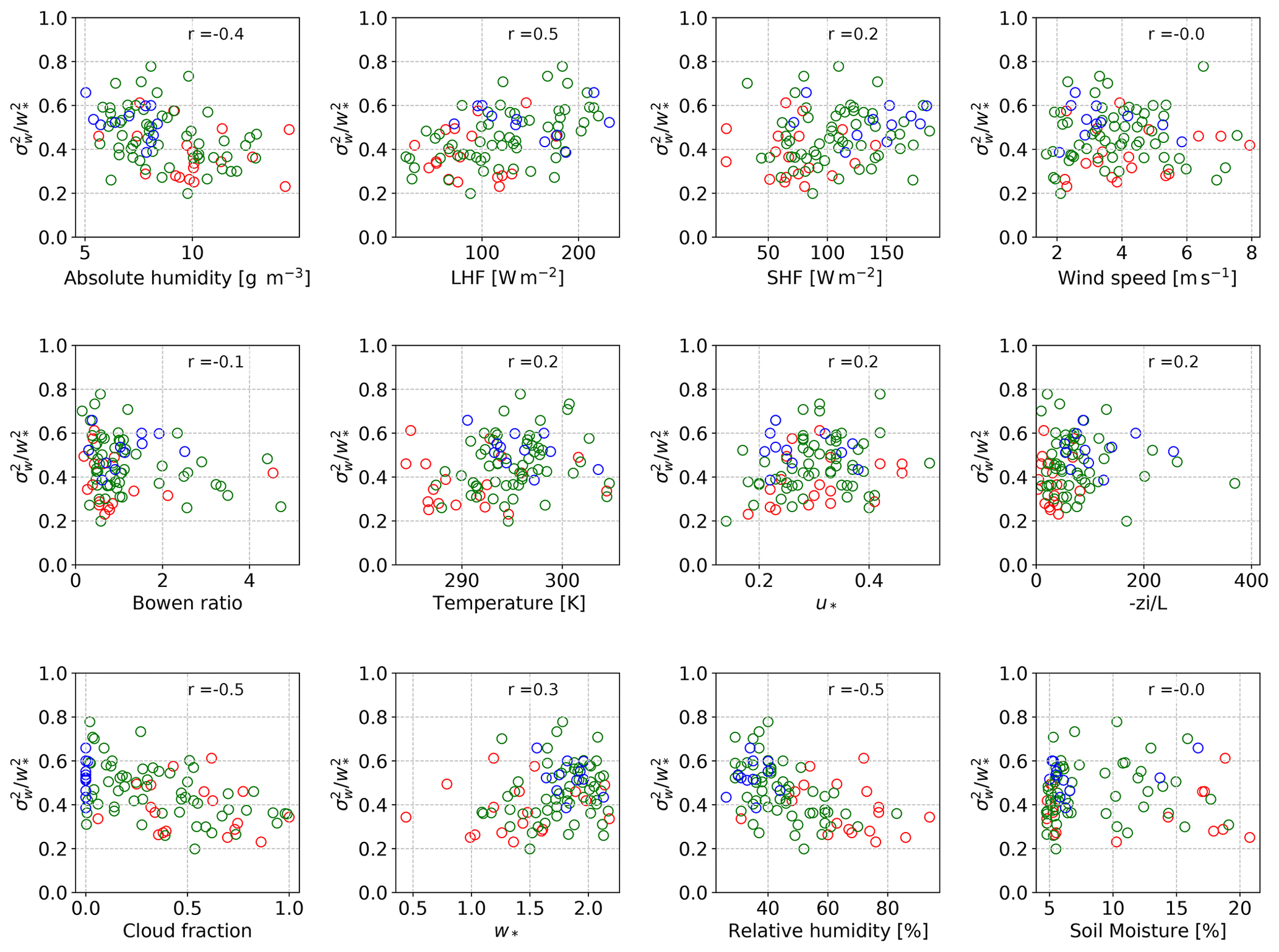
Figure 9 Scatter plots of the daily maximum values of ${\mathit{\sigma }}_w^{\mathrm{2}}/w_{*}^{\mathrm{2}}$ below 0.6 z_i and the typical meteorological parameters describing the state of the atmospheric boundary layer. The blue dots represent the data on clear-sky days, green dots represent the data on cloud-topped days and red dots represent the data on rainy days.

To investigate the origin of the variability between the clear-sky and cloud-topped days, we look in more detail at how the ${\mathit{\sigma }}_w^{\mathrm{2}}/w_{*}^{\mathrm{2}}$ depends on different meteorological parameters, taking the maximum values below 0.6 z_i of the ${\mathit{\sigma }}_w^{\mathrm{2}}/w_{*}^{\mathrm{2}}$ profiles as shown in Fig. 9. The parameters related to moisture such as latent heat flux, relative humidity, absolute humidity and cloud fraction show an absolute correlation higher than 0.4. In the following section, we present the dependency of the ${\mathit{\sigma }}_w^{\mathrm{2}}/w_{*}^{\mathrm{2}}$ profiles on the meteorological parameters particularly as mentioned above.

4.2 Factors that control the vertical velocity variance

4.2.1 Clear-sky boundary layer

The variability of the daily ${\mathit{\sigma }}_w^{\mathrm{2}}/w_{*}^{\mathrm{2}}$ profiles over the 11 clear-sky days shows a clear distinction between the datasets of the 2 years, 2020 and 2021 (Fig. 10a). We found that this distinction results from a significant difference in the surface Bowen ratio (BR) between the 2020 and 2021 datasets as shown in Fig. 10b. In the 2020 dataset, the Bowen ratio value is larger (BR higher than about 1) compared to the 2021 dataset (BR lower than 1), indicating drier surface conditions in 2020. In the dataset with the lower Bowen ratio, the magnitude of ${\mathit{\sigma }}_w^{\mathrm{2}}/w_{*}^{\mathrm{2}}$ is lower, and vice versa. One exception is a single case on 31 May 2021 which was most likely driven by synoptic-scale patterns. Other meteorological parameters, such as the bulk stability and friction velocity, do not show any systematic influence on ${\mathit{\sigma }}_w^{\mathrm{2}}/w_{*}^{\mathrm{2}}$. Within these clear-sky days, the bulk stability parameter falls in the range between $-z_i/L$ = 52 and $-z_i/L$ = 258, and the friction velocity has a range of 0.21–0.38 m s⁻¹.

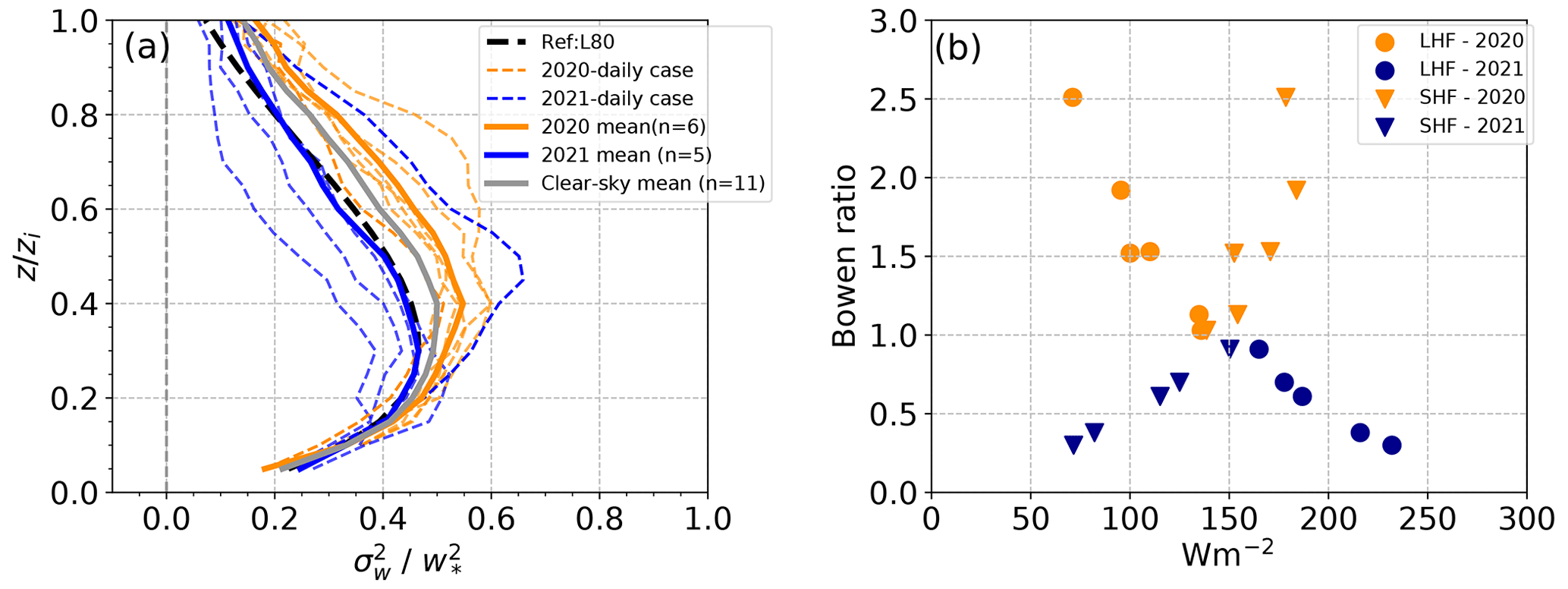
Figure 10 (a) ${\mathit{\sigma }}_w^{\mathrm{2}}/w_{*}^{\mathrm{2}}$ profiles averaged from 10:00–15:00 UTC by individual days in the clear-sky category and (b) surface sensible heat flux (triangle) and surface latent heat flux (circle) for the 2020 (orange) and the 2021 (blue) datasets.

4.2.2 Cloud-topped boundary layer

In the previous section, a good correlation is shown between absolute humidity, latent heat flux, cloud fraction, relative humidity and the daily average of ${\mathit{\sigma }}_w^{\mathrm{2}}/w_{*}^{\mathrm{2}}$ (Fig. 9). Based on these significant parameters, we further classify the cloud-topped days by cloud fraction, surface latent heat flux, absolute humidity, relative humidity and additionally surface sensible heat flux to demonstrate how the normalization by w_* leads to similar profiles and Bowen ratio to compare the behaviour with the profiles analysed in the clear-sky days. For each parameter, we defined three subcategories based on the 33 % percentile and 67 % percentile of the parameter values.

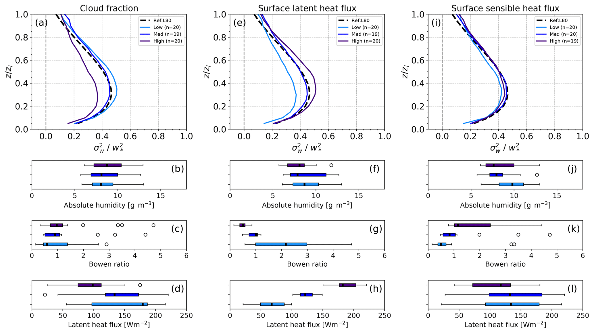
Figure 11 Vertical profiles of ${\mathit{\sigma }}_w^{\mathrm{2}}/w_{*}^{\mathrm{2}}$ averaged based on different classifications: (a) cloud fraction, (e) surface latent heat flux and (i) surface sensible heat flux. In the box plots, the corresponding values of relative humidity (b, f, j), Bowen ratio (c, g, k) and surface latent heat flux (d, h, l) for each classification are shown. The number of days (n) in each category are added in the legend.

Figure 11a shows the profiles of ${\mathit{\sigma }}_w^{\mathrm{2}}/w_{*}^{\mathrm{2}}$ averaged over the days that fall into three ranges of cloud fraction,with 0.17 and 0.48 as threshold values. As the cloud fraction increases, the ${\mathit{\sigma }}_w^{\mathrm{2}}/w_{*}^{\mathrm{2}}$ magnitude becomes smaller. The Bowen ratio and absolute humidity do not significantly differ between the three cloud fraction ranges. In the case of high cloud fraction, the surface latent heat flux value is lower, while the two other categories do not show such a clear distinction in the surface latent heat flux.

As one of the driving factors of the turbulence, the dependency of ${\mathit{\sigma }}_w^{\mathrm{2}}/w_{*}^{\mathrm{2}}$ on the surface heat flux is investigated. The profiles of ${\mathit{\sigma }}_w^{\mathrm{2}}/w_{*}^{\mathrm{2}}$ are similar in the different categories based on the sensible heat flux (Fig. 11i). This is an expected result, since the sensible heat flux is the main source of buoyancy accounted for in the definition of w_*. Since the contribution of the latent heat flux to w_* is negligible compared to the contribution of sensible heat flux, we examined if there is any remaining dependency of the normalized profiles to the latent heat flux, as suggested the Fig. 9. The collected data are divided into three categories: low (LHF < 100 W m⁻²), medium (100 W m⁻² ≤ LHF < 150 W m⁻²) and high (LHF ≥ 150 W m⁻²) latent heat flux. Figure 11e shows that the ${\mathit{\sigma }}_w^{\mathrm{2}}/w_{*}^{\mathrm{2}}$ profiles systematically increase from low to high surface latent heat flux. This is consistent with the result of the cloud fraction classification, where lower ${\mathit{\sigma }}_w^{\mathrm{2}}/w_{*}^{\mathrm{2}}$ values are also associated with lower surface latent heat flux values. In this case, the absolute humidity does not significantly differ in the three latent heat flux categories. It is interesting to observe that the Bowen ratio only has values higher than 1 if the surface latent heat flux is lower than the selected threshold of 100 W m⁻². This implies that the high Bowen ratio values result primarily from a low surface latent heat flux rather than from high values of the surface sensible heat flux.

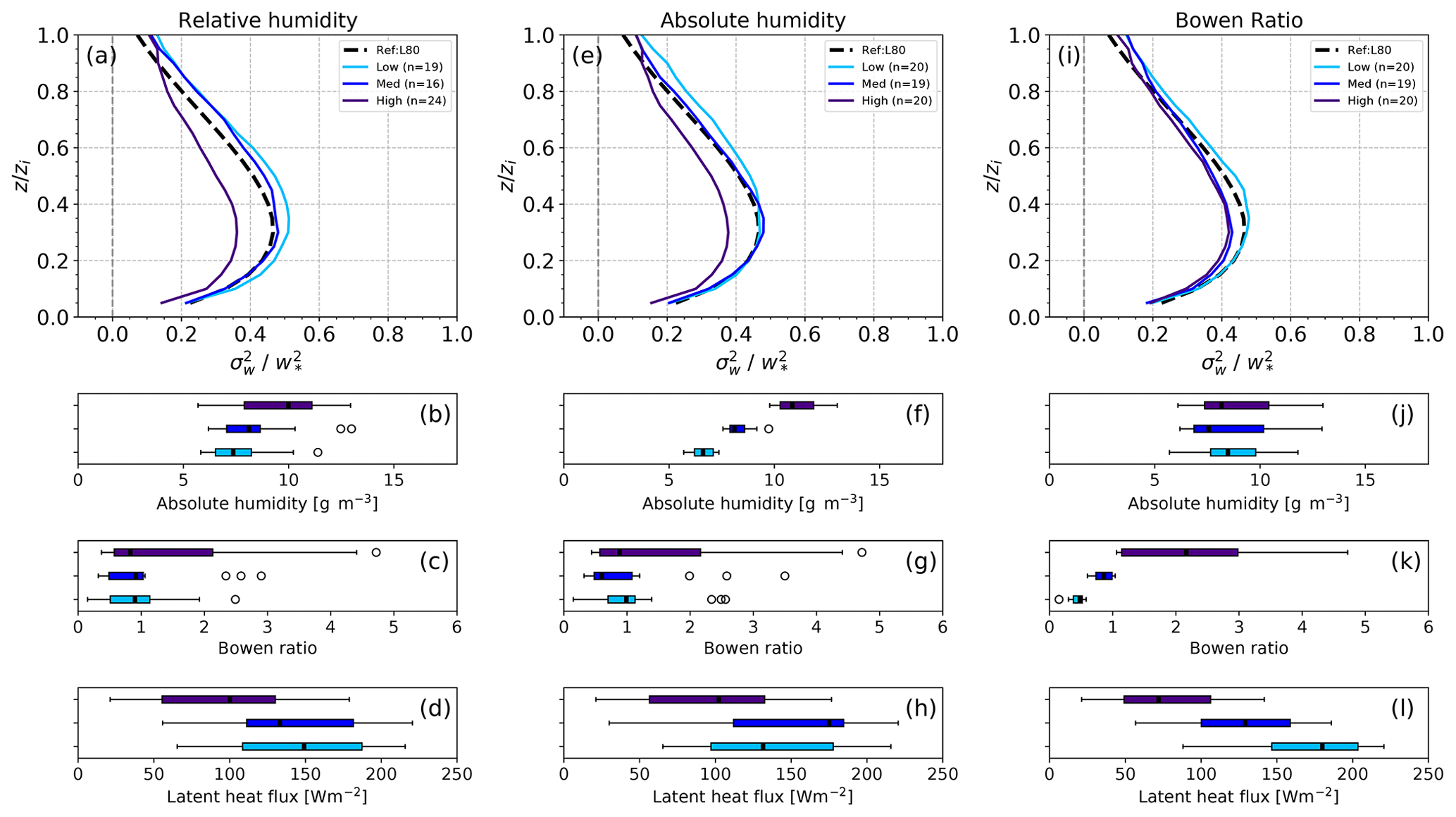
Figure 12 Similar as in Fig. 11 but for (a) relative humidity, (e) absolute humidity and (i) Bowen ratio.

Figure 12a shows the ${\mathit{\sigma }}_w^{\mathrm{2}}/w_{*}^{\mathrm{2}}$ profiles averaged over days that fall into the three ranges of relative humidity with a threshold at 38 % and 45 %. The ${\mathit{\sigma }}_w^{\mathrm{2}}/w_{*}^{\mathrm{2}}$ shows a larger magnitude in the range of relative humidity below 45 %, while a lower magnitude of ${\mathit{\sigma }}_w^{\mathrm{2}}/w_{*}^{\mathrm{2}}$ is found in the high relative humidity range. This pattern can also be seen in the clear-sky, cloud-topped and rainy day comparison in Fig. 8 and also in the cloud fraction classification Fig. 11a.

We have also examined the dependency of the variance profiles on absolute humidity as shown in Fig. 12e. Three categories of absolute humidity are defined with a threshold at 8 g m⁻² and 10.4 g m⁻². The ${\mathit{\sigma }}_w^{\mathrm{2}}/w_{*}^{\mathrm{2}}$ profiles in the low and medium absolute humidity categories have a similar magnitude below 0.4 z_i. Above 0.4 z_i, the low absolute humidity category is characterized by a higher magnitude of ${\mathit{\sigma }}_w^{\mathrm{2}}/w_{*}^{\mathrm{2}}$. This similar behaviour is also shown in the surface latent heat flux, where a similar range of values is found in the low and medium categories. As expected, the lower magnitude of ${\mathit{\sigma }}_w^{\mathrm{2}}/w_{*}^{\mathrm{2}}$ falls in the high absolute humidity category, which we can also see in the clear-sky, cloud-topped and rainy day comparison in Fig. 8.

The dependency of the averaged ${\mathit{\sigma }}_w^{\mathrm{2}}/w_{*}^{\mathrm{2}}$ on the Bowen ratio is not as clear as on clear-sky days. The ${\mathit{\sigma }}_w^{\mathrm{2}}/w_{*}^{\mathrm{2}}$ profiles averaged over the days with high and medium Bowen ratio are similar, while the days with a lower Bowen ratio have a higher magnitude of ${\mathit{\sigma }}_w^{\mathrm{2}}/w_{*}^{\mathrm{2}}$ (Fig. 12i). In the cloud-topped boundary layer, the dependency of the profiles on the Bowen ratio is opposite to the dependency found on clear-sky days. This could be the result of a significantly higher relative humidity on cloud-topped days, as the magnitude of ${\mathit{\sigma }}_w^{\mathrm{2}}/w_{*}^{\mathrm{2}}$ is lower in the case of higher relative humidity.

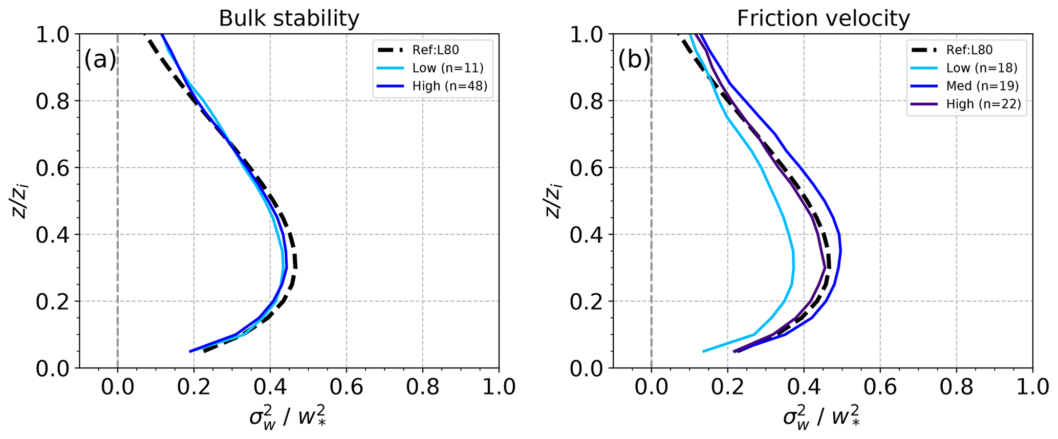
Figure 13 Classification of ${\mathit{\sigma }}_w^{\mathrm{2}}/w_{*}^{\mathrm{2}}$ based on the (a) bulk stability and (b) friction velocity. In the legend, n indicates the number of days in each class.

We did not find any considerable dependency of ${\mathit{\sigma }}_w^{\mathrm{2}}/w_{*}^{\mathrm{2}}$ on other parameters used to characterize turbulence, such as bulk stability. We used the bulk stability, $-z_i/L$, where L is the Obukhov length. The same threshold as in Lenschow et al. (2012) is applied with $-z_i/L<\mathrm{30}$ for the less unstable and $-z_i/L\ge \mathrm{30}$ for the more unstable category. From the total of 59 d used for this case, 11 d are in the less unstable category, and 48 d are in the more unstable category. Even though the range of the values of the stability parameter is similar to the range in Lenschow et al. (2012), we found similar profiles of ${\mathit{\sigma }}_w^{\mathrm{2}}/w_{*}^{\mathrm{2}}$ in the two categories (Fig. 13). On the other hand, there is a dependency of ${\mathit{\sigma }}_w^{\mathrm{2}}/w_{*}^{\mathrm{2}}$ on the friction velocity (u_*); however it does not show a systematic pattern. The ${\mathit{\sigma }}_w^{\mathrm{2}}/w_{*}^{\mathrm{2}}$ profiles are divided into three categories based on the friction velocity with a threshold at 0.28 and 0.34 m s⁻¹. The lowest magnitude of ${\mathit{\sigma }}_w^{\mathrm{2}}/w_{*}^{\mathrm{2}}$ is found for the low friction velocity, while the highest magnitude of ${\mathit{\sigma }}_w^{\mathrm{2}}/w_{*}^{\mathrm{2}}$ is found for the medium friction velocity.

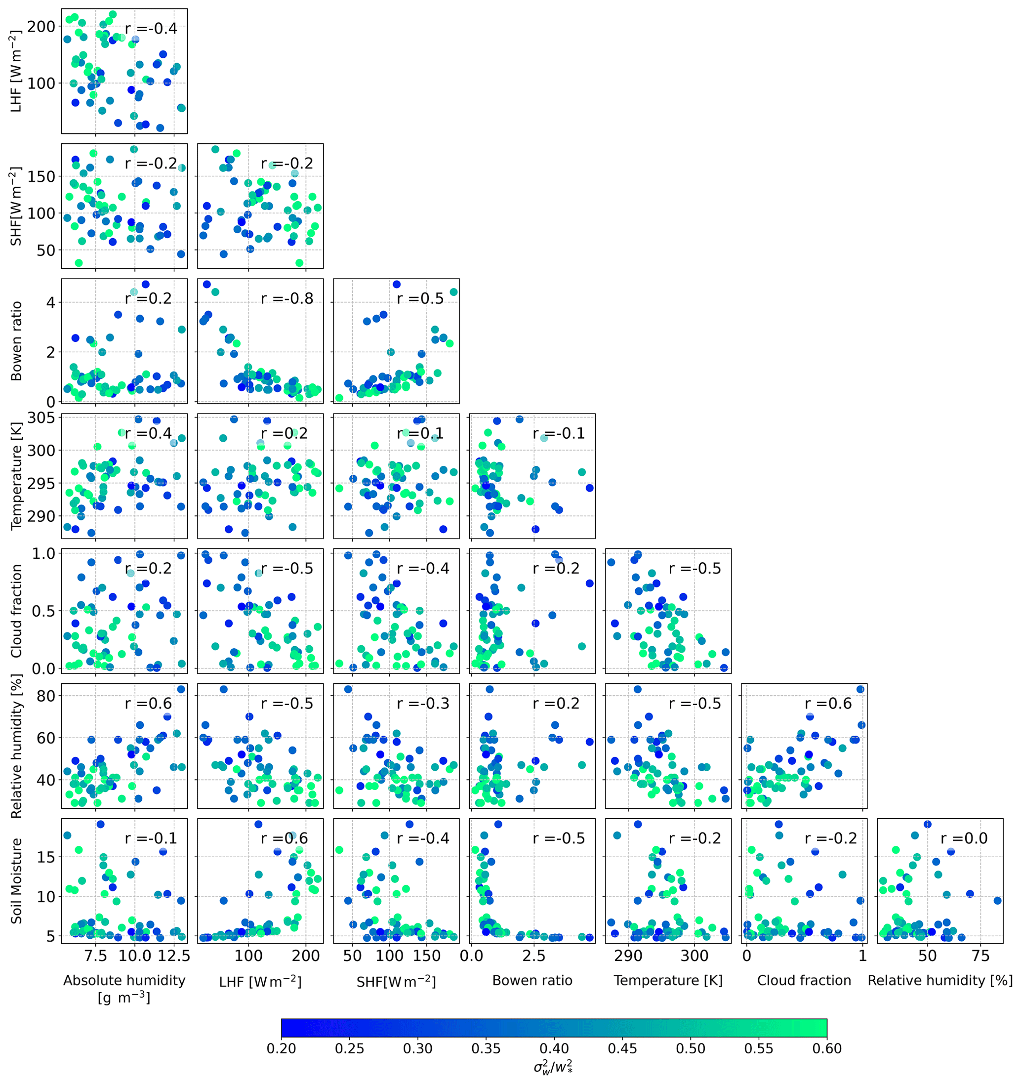
Figure 14 Correlation matrix of seven meteorological parameters, with colour representing the maximum value of the daily average of ${\mathit{\sigma }}_w^{\mathrm{2}}/w_{*}^{\mathrm{2}}$ below 0.6 z_i.

To complete the analysis, we have further investigated the joint dependency between the meteorological parameters analysed above as shown by the correlogram in Fig. 14. The dots are coloured by the maximum value of ${\mathit{\sigma }}_w^{\mathrm{2}}/w_{*}^{\mathrm{2}}$ below 0.6 z_i to demonstrate bivariate changes in ${\mathit{\sigma }}_w^{\mathrm{2}}/w_{*}^{\mathrm{2}}$, and the coefficient correlation indicates the correlation between two parameters. We found a good joint dependency of ${\mathit{\sigma }}_w^{\mathrm{2}}/w_{*}^{\mathrm{2}}$ where relative humidity is one of the examined parameters. However, relative humidity is also dependent on temperature, which complicates the interpretation of the observed dependencies of ${\mathit{\sigma }}_w^{\mathrm{2}}/w_{*}^{\mathrm{2}}$. As expected, the latent heat flux shows a high correlation with soil moisture, absolute humidity and cloud fraction. Although the data are scattered, we still can see the trend of ${\mathit{\sigma }}_w^{\mathrm{2}}/w_{*}^{\mathrm{2}}$ on the joint-parameter scatter plots. The joint parameters which show a clear trend in ${\mathit{\sigma }}_w^{\mathrm{2}}/w_{*}^{\mathrm{2}}$ are aligned with the parameters that we used for the ${\mathit{\sigma }}_w^{\mathrm{2}}/w_{*}^{\mathrm{2}}$ profile analysis in this section, which further strengthens our conclusions.

5 Discussion

Daily averaged profiles of ${\mathit{\sigma }}_w^{\mathrm{2}}/w_{*}^{\mathrm{2}}$ on clear-sky days are strongly related to the values of the surface Bowen ratio. Since the profiles are normalized by the convective velocity scale (w_*), the dependency of ${\mathit{\sigma }}_w^{\mathrm{2}}/w_{*}^{\mathrm{2}}$ on the surface Bowen ratio is introduced through the changes in the surface latent heat flux and cannot be explained by the generation of turbulence by buoyancy. The ${\mathit{\sigma }}_w^{\mathrm{2}}/w_{*}^{\mathrm{2}}$ was lower during days with a higher surface latent heat flux and vice versa. This suggests that a higher flux of moisture from the land surface might place a limit on the strength of convective circulations that maybe act as a dehumidifier of the boundary layer in these cases similar to the case of deep convection (Pauluis and Held, 2002); however, this is only a speculation and needs further investigation. One outlier in the clear-sky 2021 dataset, 31 May 2021, shows a larger ${\mathit{\sigma }}_w^{\mathrm{2}}/w_{*}^{\mathrm{2}}$ with maximum values at 0.5 z_i. Compared to the other sample days in 2021, a higher soil moisture content, around 17 %, is found on that day, while all other days had a soil moisture content well below 14 %. We also observed a higher magnitude of the mean ${\mathit{\sigma }}_w^{\mathrm{2}}/w_{*}^{\mathrm{2}}$ on clear-sky days compared to the result in the study of Berg et al. (2017), which focuses on clear-sky days in a year-long dataset, and also the study of Lareau et al. (2018), which included clear-sky days.

We looked into the dependency of ${\mathit{\sigma }}_w^{\mathrm{2}}/w_{*}^{\mathrm{2}}$ on cloud fraction, as the previous studies showed contrasting results. We found that the magnitude of ${\mathit{\sigma }}_w^{\mathrm{2}}/w_{*}^{\mathrm{2}}$ decreased with an increase in cloud fraction, which is the opposite to the results of the previous studies. While Hogan et al. (2009) found no significant difference between ${\mathit{\sigma }}_w^{\mathrm{2}}/w_{*}^{\mathrm{2}}$ on clear-sky and cloud-topped days, Chandra et al. (2010) found higher ${\mathit{\sigma }}_w^{\mathrm{2}}/w_{*}^{\mathrm{2}}$ on days with a higher cloud fraction. On the other hand, Lareau et al. (2018) found the highest ${\mathit{\sigma }}_w^{\mathrm{2}}/w_{*}^{\mathrm{2}}$ on days with an intermediate cloud fraction. Our results thus confirm the conclusion made in Hogan et al. (2009) that boundary layer clouds are not a relevant source of turbulence in the convective boundary layer; moreover, our results suggest the opposite, that the formation of clouds acts as a sink rather than a source of turbulence. A similar dependency is also found in the comparison between clear-sky, cloud-topped and rainy days, with the magnitude of ${\mathit{\sigma }}_w^{\mathrm{2}}/w_{*}^{\mathrm{2}}$ decreasing from clear-sky to rainy days.

The results of our study related to cloud-topped days should not be generalized to other locations or seasons. The development of boundary layer clouds involves a number of complex and competing mechanisms of the land–atmosphere system. These interactions manifest in a non-linear dependency of cloud development on the state of soil moisture. So, for example, if the atmospheric stability above the boundary layer is strong, soil moisture acts to support the cloud development. However, if the atmospheric stability is weak, clouds will be favoured over dry soils, while the increase of soil moisture will act to decrease the probability of cloud development (Ek and Holtslag, 2004; Gentine et al., 2013). The intensity of convective updrafts that form the clouds is thus more likely related to the state of soil moisture and the magnitude of the surface heat fluxes and not the cloud fraction itself. Although we could not find a good agreement between the magnitude of ${\mathit{\sigma }}_w^{\mathrm{2}}/w_{*}^{\mathrm{2}}$ and a single measurement of soil moisture under the invariant soil moisture regime at the Falkenberg site within the time period of the analysis, the soil moisture seems to have an indirect impact through the moisture transport as shown by the surface heat flux analysis. So, differences in the type of soil and climate regime might explain the differences between the results for the Lindenberg observatory and those for the ARM SGP site, the two observational sites that have a very distinct regime of soil moisture: the first one is generally abundant in soil moisture, while the second one is in a semi-arid regime (Koster et al., 2004).

The contrasting results in the dependency of ${\mathit{\sigma }}_w^{\mathrm{2}}/w_{*}^{\mathrm{2}}$ on the surface Bowen ratio on clear-sky and cloud-topped days in our study (Figs. 10 and 12i) can be explained by the compounding dependency of ${\mathit{\sigma }}_w^{\mathrm{2}}/w_{*}^{\mathrm{2}}$ on relative humidity. During the clear-sky days, the relative humidity at 10 m was in a narrow range of 26 %–43 %, while on the cloud-topped days, this range was much wider, 28 %–77 %.

6 Conclusions

In this study, the dependency of the normalized vertical velocity variance, ${\mathit{\sigma }}_w^{\mathrm{2}}/w_{*}^{\mathrm{2}}$, on the meteorological conditions in the convective boundary layer is studied statistically during the summer periods (May–August) of the 2 consecutive years of the FESSTVaL 2020/21 field experiment. The mean day-to-day profiles were calculated from the raw Doppler lidar data at 1.5–3 s resolution averaged over 30 min during the convective time of the day with a well developed boundary layer.

Similar to previous studies, we found that the mean ${\mathit{\sigma }}_w^{\mathrm{2}}/w_{*}^{\mathrm{2}}$ profile of all of the selected days is similar to the universal profile of Lenschow et al. (1980). However, daily mean profiles also show a high day-to-day scatter after normalization using the square of the convective velocity scale ($w_{*}^{\mathrm{2}}$). To investigate where this residual scatter originates from, we categorized the ${\mathit{\sigma }}_w^{\mathrm{2}}/w_{*}^{\mathrm{2}}$ profiles into two levels: first we distinguished between clear-sky, cloud-topped and rainy days, and second, for the clear-sky and cloud-topped days, we applied an additional level of categorization based on the relevant meteorological parameters.

The magnitude of the mean ${\mathit{\sigma }}_w^{\mathrm{2}}/w_{*}^{\mathrm{2}}$ profile is highest during clear-sky days and systematically decreases for the cloud-topped and rainy days. We found that this change in the magnitude of ${\mathit{\sigma }}_w^{\mathrm{2}}/w_{*}^{\mathrm{2}}$ follows changes in the mean of absolute humidity in the boundary layer and the surface latent heat flux: ${\mathit{\sigma }}_w^{\mathrm{2}}/w_{*}^{\mathrm{2}}$ is lower in the case of a higher absolute humidity and lower surface latent heat flux, and vice versa. However, the distinction in the absolute humidity values between cloud-topped and rainy days could not be made, although the variance profiles did show a significant difference in magnitude and their shape. This result suggests that the content of water vapour in the boundary layer and the vertical transport of moisture could explain most of the scatter in the observed profiles of ${\mathit{\sigma }}_w^{\mathrm{2}}/w_{*}^{\mathrm{2}}$ on the clear-sky days and cloud-topped days. Since this dependency is a reversed one, the moisture content and the vertical transport of moisture are limiting factors on the intensity of turbulence in the convective boundary layer.

We further investigated the ${\mathit{\sigma }}_w^{\mathrm{2}}/w_{*}^{\mathrm{2}}$ profiles in two of the main categories, the clear-sky and the cloud-topped days, separately. Since the effect of buoyancy is already taken into account in the scaling parameter w_*, we investigated other relevant meteorological parameters of the convective boundary layer.

In the clear-sky boundary layer, two regimes are found in the 2 different years, a low Bowen ratio regime with lower ${\mathit{\sigma }}_w^{\mathrm{2}}/w_{*}^{\mathrm{2}}$ and a high Bowen ratio regime with higher ${\mathit{\sigma }}_w^{\mathrm{2}}/w_{*}^{\mathrm{2}}$ magnitudes. These differences in ${\mathit{\sigma }}_w^{\mathrm{2}}/w_{*}^{\mathrm{2}}$ and its dependency on the Bowen ratio are driven by differences in the surface latent heat flux in the 2 years. Besides the Bowen ratio and the surface latent heat flux, the ${\mathit{\sigma }}_w^{\mathrm{2}}/w_{*}^{\mathrm{2}}$ profiles did not show any robust sensitivity to other parameters such as bulk stability or friction velocity under clear-sky conditions.

On the cloud-topped days, a systematic change of the ${\mathit{\sigma }}_w^{\mathrm{2}}/w_{*}^{\mathrm{2}}$ profiles is found for changes in the cloud fraction, surface latent heat flux, absolute humidity and Bowen ratio. We found no dependency of the ${\mathit{\sigma }}_w^{\mathrm{2}}/w_{*}^{\mathrm{2}}$ profiles on the bulk stability, while the highest ${\mathit{\sigma }}_w^{\mathrm{2}}/w_{*}^{\mathrm{2}}$ is found at the intermediate friction velocity (u_*) values. However, scaling of ${\mathit{\sigma }}_w^{\mathrm{2}}$ using a modified convective velocity that accounts for the effects of wind shear (Moeng and Sullivan, 1994) did not significantly reduce the variability of the daily profiles compared to the scaling using the square of the convective velocity scale ($w_{*}^{\mathrm{2}}$).

Based on our results and the comparison to previous studies, we conclude that a systematic and robust dependency of ${\mathit{\sigma }}_w^{\mathrm{2}}/w_{*}^{\mathrm{2}}$ on cloud fraction across different locations and seasons could not be expected. This relationship will depend on the soil moisture regime because of a complex interplay of multiple competing mechanisms of land–atmosphere interaction that leads to the formation of clouds. Therefore, the cloud fraction is not an adequate parameter on its own for investigating the day-to-day variability of ${\mathit{\sigma }}_w^{\mathrm{2}}/w_{*}^{\mathrm{2}}$ profiles.

Our study confirms the conclusion made in Hogan et al. (2009) that shallow clouds are not a relevant source of turbulence in the convective boundary layer. Moreover, we find that the intensity of turbulence reduces with an increase in the fraction of boundary layer clouds, except in the cloud layer between approximately 0.9 z_i and z_i.

The results of our study have an implication for the development of parameterizations of boundary layer turbulence and convection. The convective velocity scale, w_*, frequently used in these parameterizations does not account for important factors that control the intensity of turbulence in the convective boundary layer, expressed through the variance of vertical velocity. To improve these parameterizations, a new scaling law has to be developed that will take into account the influence of moisture transport from the land surface to the atmosphere, the water content in the boundary layer and development of boundary layer clouds that is highly controlled by the state of the land surface.