Capturing synoptic-scale variations in surface aerosol pollution using deep learning with meteorological data

The estimation of daily variations in aerosol concentrations using meteorological data is meaningful and challenging, given the need for accurate air quality forecasts and assessments. In this study, a 3×50-layer spatiotemporal deep learning (DL) model is proposed to link synoptic variations in aerosol concentrations and meteorology, thereby building a “deep” Weather Index for Aerosols (deepWIA). The model was trained and validated using 7 years of data and tested in January–April 2022. The index successfully reproduced the variation in daily PM_2.5 observations in China. The coefficient of determination between PM_2.5 concentrations calculated from the index and observation was 0.72, with a root mean square error (RMSE) of 16.5 µg m⁻³. The DeepWIA performed better than Weather Forecast and Research (WRF)-Chem simulations for eight aerosol-polluted cities in China. The simulating power of the model also outperformed commonly used PM_2.5 concentration retrieval models based on random forest (RF), extreme gradient boost (XGB), and multilayer perceptron (MLP). The index and the DL model can be used as robust tools for estimating daily variations in aerosol concentrations.

1 Introduction

Meteorology and emissions drive variations in aerosol concentrations, with the latter strongly modulating seasonality and long-term trends (Q. Zhang et al., 2019; Wang et al., 2011) but remaining stable at synoptic scales, excluding unexpected events such as volcanic activity and emergency lockdowns. Meteorology dominates synoptic scale (i.e., high-frequency) variations in aerosol concentrations (Bei et al., 2016; Zheng et al., 2015; Leung et al., 2018) and regulates aerosol physicochemical processes including their generation, diffusion, transport, and deposition (Feng et al., 2016), thus synchronizing periodic accumulation–removal of aerosol pollution with activities of synoptic systems (Chen et al., 2008; Guo et al., 2014).

Air quality forecasts and emission-reduction evaluations require the estimation of aerosol concentrations and their variations from meteorological data. The strong impacts of meteorology on physicochemical processes make such estimation possible. Chemical transport models (CTMs) can be used as a tool for this purpose. Given an emission inventory, CTMs aim to detail the physicochemical processes and simulate variations in aerosol concentrations over all timescales. The CTM-based simulations provide information on intermediate processes, allowing convenient analysis of mechanisms of aerosol pollution. However, uncertainties in parameterization and emission inventories lead to significant estimation errors in aerosol concentrations (Zhong et al., 2016; Zhang et al., 2016, 2018). Taking the commonly used Weather Forecast and Research (WRF)-Chem model as an example, Sicard et al. (2021) reported a Pearson correlation coefficient of 0.44 (equivalent to a coefficient of determination (R²) of ∼0.2) between simulated and observed daily surface PM_2.5 (particle matter of diameter < 2.5 µm) concentrations in China, based on a resolution simulation of 8 km in 2015. Another WRF-Chem simulation over 2014–2015 gave a better R² value of 0.44 for a smaller WRF-Chem simulation domain over 131 cities in eastern China (Zhou et al., 2017). In addition, the complexity of CTMs requires large computational resources.

Data-based models provide another estimation tool, using historical datasets to establish empirical or semiempirical models linking meteorology and aerosol concentrations without a description of intermediate processes. A data-based model requires negligible computational resources compared with CTMs. In China, two semiempirical meteorological indices are used for daily variations in aerosol concentrations, the Parameter Linking Air quality to Meteorological conditions (PLAM; Yang et al., 2016) and Air Stagnation Index (ASI; Feng et al., 2018, 2020b). Both indices include an extra “background factor” describing the effects of slowly changing emissions and regional differences. However, the weak nonlinear fitting power of these meteorological indices makes it difficult to beat CTMs for daily aerosol concentration estimation. In addition, such simple meteorological indices cannot be applied to a large region such as the whole of China (Sect. 4).

As machine learning (ML) and deep learning (DL) are approaches to promoting the nonlinear fitting power of data-based models, it is possible to establish an ML/DL model for variations in aerosol concentrations. The ML/DL-based observation retrieval for PM_2.5 concentration has become very popular (Yuan et al., 2020). Estimations in such studies use satellite-based aerosol optical depth (AOD; Wei et al., 2019a, 2020; Geng et al., 2021; Li et al., 2020) or surface visibility observations (Zhong et al., 2021; Gui et al., 2020) as “primary” data and meteorological variables and other quasistatic data (e.g., topography, population, emissions) as “auxiliary” data, with these being fed into a generic ML/DL model to estimate PM_2.5 concentrations. Commonly used models include random forest (RF; Wei et al., 2019a; Geng et al., 2021), extreme gradient boost (XGB; Gui et al., 2020), and multilayer perceptron (MLP; Li et al., 2020) methods, applied individually or together (Song et al., 2021). Compared with CTM simulations and meteorological indices, the injection of observation data improves the estimation of PM_2.5 concentrations and its variations. In turn, the popularity of these studies indicates that using only meteorological data as primary data for aerosol concentrations is a challenging task, even with ML/DL.

To address this issue, two key points should be considered in model design. First, the model should focus only on the synoptic-scale variability of aerosols, as meteorology is not a predominant factor in the low-frequency variability of aerosol concentrations. Indeed, the direct fitting of aerosol concentrations misinterprets the relationship between meteorology and aerosols, possibly leading to an overfitting ML/DL model. Second, the model should include more spatiotemporal meteorological features and a more powerful nonlinear capability to cover the complex characteristics of aerosol variations over large regions such as China than previous linear and DL/ML models.

Therefore, here we propose a spatiotemporal deep neural network linking daily averaged meteorological fields and aerosol concentrations in China. Rather than fitting PM_2.5 concentrations, the DL model focuses on capturing their synoptic variations. In the DL model, daily averaged meteorological variables over 3 d and quasistatic data (as the input variables) are fused to provide a daily deep Weather Index for Aerosols (as the model output), termed “deepWIA” (the model is named “deepWIA model”). Compared with CTM-based and other data-based estimations reported in previous studies, the model efficiently reduces the estimation error in PM_2.5 concentrations over China with no significant overfitting, as often occurs in previous ML-based models.

The rest of this paper is organized as follows. Section 2 describes the deepWIA model, training data, methods of feature engineering (i.e., preprocessing to generate input variables), and results with training–validation datasets. Section 3 focuses on the performance of the model using a test dataset, with a comparison with a WRF-Chem simulation in eight heavily polluted cities. Section 4 gives a comparison with related studies. We also undertook several ablation experiments to illustrate possible reasons for the strong performance of the deepWIA model. Section 5 provides the geographic distribution of synoptic variations in aerosol pollution over the test period. Section 6 concludes the study.

2 DeepWIA model

2.1 Input variables

Input variables of the deepWIA model includes daily averaged meteorological variables from the fifth-generation European Centre for Medium-range Weather Forecasts (ECMWF) reanalysis data (ERA5), with a horizontal resolution of $\mathrm{0.25}{}^{\circ }\times \mathrm{0.25}{}^{\circ }$. Since a trained DL model can automatically select the input variables to compose the best model that fits the target variable (PM_2.5 concentrations) with activation functions, the task for feature engineering is to feed the DL model with as many variables as possible that are related to the day-to-day variation of PM_2.5 concentrations. These input variables (Table 1) can be classified into four categories as follows.

Table 1 The input variables and their corresponding categories, references and importance ranking in the deepWIA model.

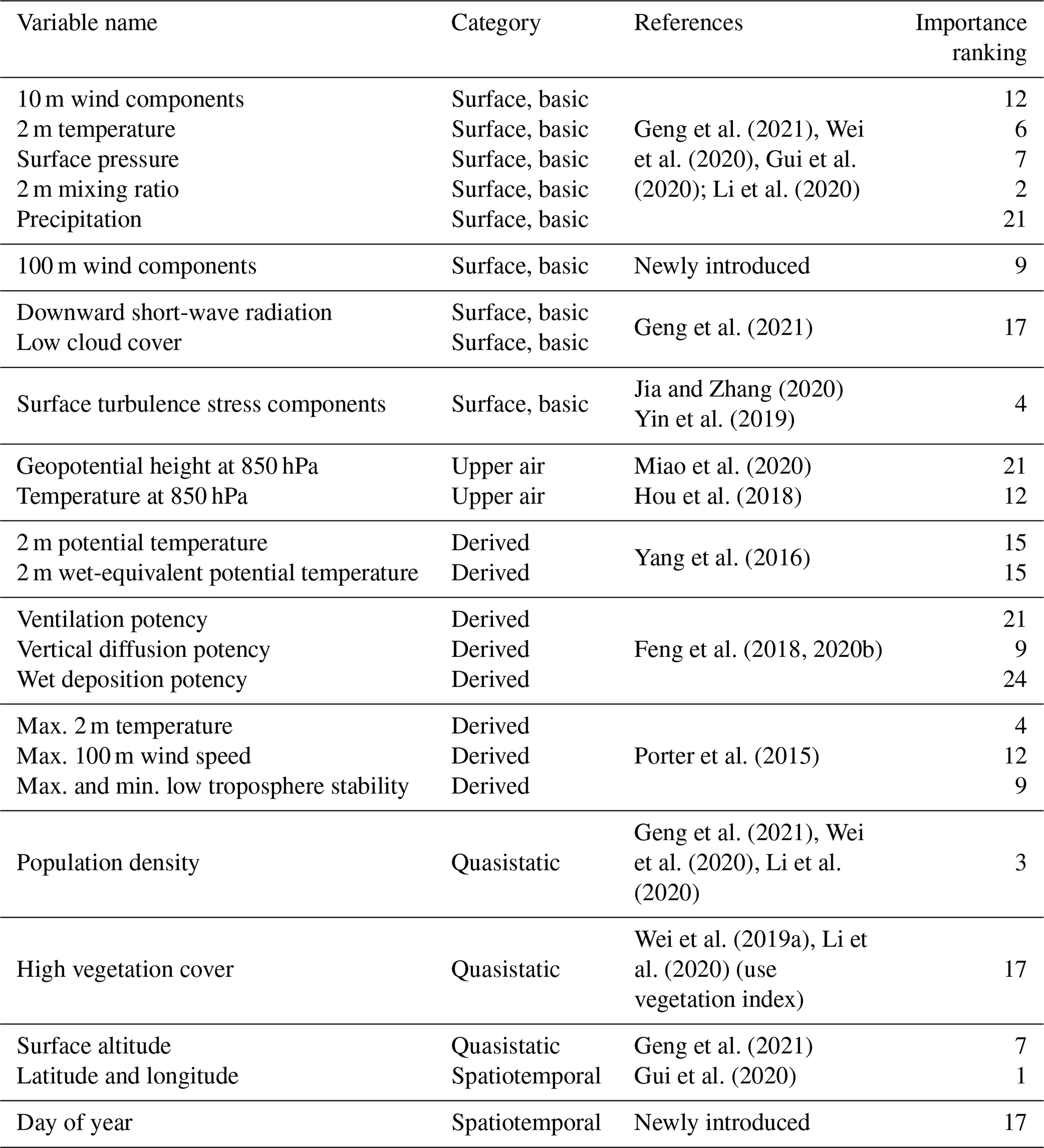
Basic meteorological variables near the surface. We use 10 m altitude wind components, 2 m temperature, surface pressure, surface downward short-wave radiation, and total precipitation, which are frequently used as input variables in ML/DL-based studies of PM_2.5 retrieval (Geng et al., 2021; Wei et al., 2020; Gui et al., 2020; Li et al., 2020). In addition, we introduce 100 m wind components and surface turbulent stress, as they are related to horizontal and vertical diffusion in the planetary boundary layer (PBL), respectively.

Meteorological fields in the upper air include geopotential height and temperature at 850 hPa. We introduce these two variables for the deepWIA model in learning the effects of synoptic patterns on aerosol variations.

Derived input variables referring to previous studies of aerosol concentration–meteorology relationships. Our model contains potential temperature and wet-equivalent potential temperature derived from PLAM, as they can identify the types of aerosol-related air masses controlling the local area (Yang et al., 2016). In addition, we introduce three kernel parameters of ASI, including ventilation potency, vertical diffusion potency, and wet deposition potency of aerosols (Feng et al., 2018). The ventilation potency illustrates the effects of wind speed in local PBL, which are simply represented by the nonlinear function of the height-weighted average of wind speed over the PBL; vertical diffusion potency is represented by the inverse of PBL height, which roughly presents the vertical diffusion range of aerosols due to turbulence; and wet deposition potency illustrates a significant decrease in the aerosol concentrations due to precipitation. The values of 0 and e correspond to precipitation greater than or equal to and less than 3 mm d⁻¹, respectively. All the formulae for these variables derived from ASI are given in the Supplement (Eqs. S1–S3l). Moreover, referring to Porter et al. (2015), we use the daily maxima and minima of low-troposphere stability (i.e., the potential temperature difference between 700 hPa and the surface) and daily maxima of 2 m temperature and of 100 m wind speed.

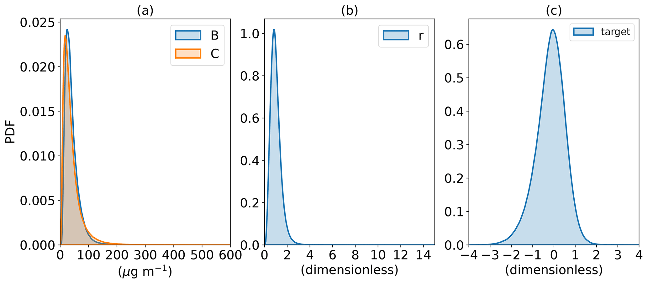
Figure 1 Probability density functions of (a) observed PM_2.5 concentrations (C, orange line) and background concentrations (B, blue line), (b) $r\left(\frac{C}{B}\right)$, and (c) $\widehat{r}$ (deepWIA target variable).

Quasistatic and spatiotemporal variables (non-meteorological variables) include population density, surface altitude, and surface high vegetation cover, which are also commonly used in PM_2.5 observation retrieval. The population density is regridded from the Gridded Population of the World (GPW) version 4 dataset at an original resolution of 1 km. Surface altitude and surface high vegetation cover are from the ERA5 datasets. These variables as well as latitude and longitude (Gui et al., 2020; Zhong et al., 2021) aid learning of the local characteristics of aerosol concentration. In addition, the model is built uniformly using all observed samples in China as the dataset (see Sect. 2.3). It is difficult for the model to obtain the correct seasonal information in the meteorological variables of these samples. Hence, we introduce seasonal information to the deepWIA model through a variable of “day of the year”, which has rarely been considered in previous models.

2.2 Target

The fitting target of the deepWIA model is not the PM_2.5 concentration per se but an index that tracks synoptic variations in PM_2.5 concentrations. Motivated by the ASI and PLAM approaches, we use the predefined form

$$\begin{array}{}\text{(1)}& r=C/B\end{array}$$

to separate the long-term background aerosol concentration, B, and synoptic variability, r, superimposed on B, where C is the daily averaged PM_2.5 concentration. We term this process “timescale separation”. B is calculated as a 31 d running average over the current year and the previous year, i.e.,

$$\begin{array}{}\text{(2)}& B={\displaystyle \frac{\mathrm{1}}{\mathrm{62}}}\left(\sum _{y-\mathrm{1}}^y\sum _{d-\mathrm{15}}^{d+\mathrm{15}}C\right),\end{array}$$

where d and y denote the date and year of the PM_2.5 sample, respectively. The seasonality, the long-term trend in emissions and local characteristics of each sample are contained in B, and r, estimated from meteorological data, indicates the effect of weather on high-frequency variations in PM_2.5 concentrations. It should be noted that the timescale of the running average is not a sensitive parameter for the performance of the deepWIA model. When a new model with the same structure, input variables, and training method as the original deepWIA model, but with a 61 d running average for the current year and the previous year as the background is used, the model performance is close to the original one using the background value with 31 d running averaged (see Fig. S1 in the Supplement).

Target data imbalance is an issue of concern. Previous studies have shown that PM_2.5 concentrations have an extremely asymmetric long-tailed probability distribution function (PDF; Lu, 2002; Feng et al., 2018). The number of samples with low and medium values is much larger than that for high values (Fig. 1); r has a similar PDF, with values of 0–15, but concentrated mainly between 0 and 2. Such a distribution would weaken the performance of a data-based model, as it is difficult for such a model to discern small differences among low-value samples. To mitigate such data imbalance, the fitting target (i.e., the deepWIA, labeled $\widehat{r}$) of our model is defined as

$$\begin{array}{}\text{(3)}& \widehat{r}={\log }_{\mathrm{2}}r.\end{array}$$

This label transformation maintains the value of the target between −4 and 4 (Fig. 1c), giving a meaningful weather index for aerosol, with positive and negative values denoting aerosol-pollution days and clean days, respectively. For example, $\widehat{r}=+\mathrm{1}$ and −1 mean that the PM_2.5 concentrations will be 2 times (i.e., 2¹) and $\mathrm{1}/\mathrm{2}$ of (i.e., 2⁻¹) the background concentration B, respectively.

National surface PM_2.5 observations are from the real-time air quality platform (https://air.cnemc.cn:18007, last access: 3 August 2022) of the China National Environmental Monitoring Center. This platform has published air quality data since 2013. We use data from 2015 because the number of observation sites since that year exceeds 1000, with a widespread distribution across the country, making the sample more representative. Furthermore, the number of PM_2.5 observation sites within different ERA5 grid cells is uneven, which would also undermine the representativeness of the sampling. Therefore, we use gridded observations, with the PM_2.5 observation in a grid cell being the mean of all observations within that cell.

2.3 Model description

Aerosol concentrations at specific times and locations depend on local and surrounding meteorological fields over the current and past few days, as CTMs indicate. Therefore, we designed the deepWIA model as a spatiotemporal neural network (Fig. 2).

Figure 2 Backbone architecture of the deepWIA model.

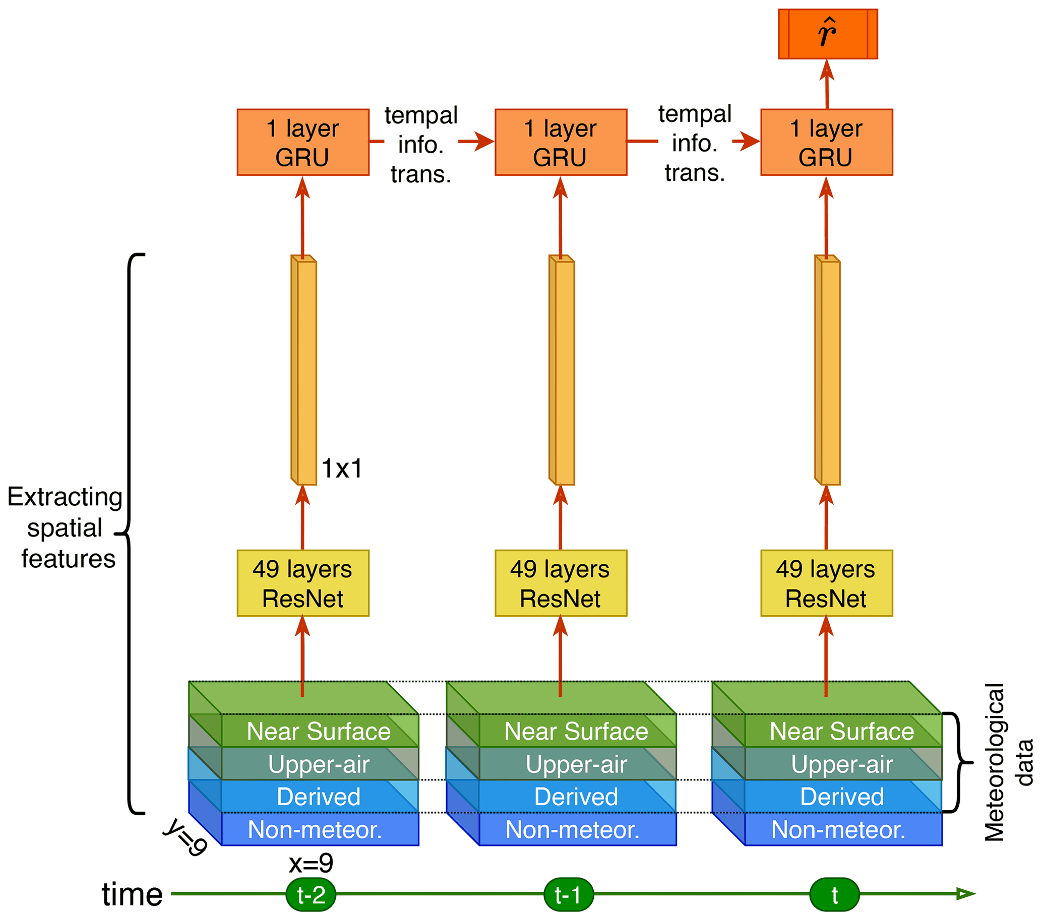
The spatial module of the model is based on residual network (ResNet; He et al., 2016). At each time step (i.e., day), the module can extract the information of the input variable and its spatial pattern within 9×9 ERA5 grid cells (about 200×200 km in China) around each observation sample point. We chose such a 9×9 sampling grid cell with reference to Feng et al. (2020b) and the limitations of our computational resources. The ResNet has a structure similar to that of the classical ResNet-50 (He et al., 2016), but only 49 convolution layers and a maximum of 512 channels (i.e., variables in convolution layers). These convolution layers of the ResNet automatically reorganize the input variables into multiple features associated with the target (i.e., PM_2.5 concentrations). This ResNet does not have the final pooling (i.e., spatial average) layer of the original ResNet-50, because a sample over the 9×9 ERA5 grid cell has shrunk to a scalar spatially after 49 convolution layers. The number of channels is also less than the traditional ResNet-50 due to our computational resource limitation. And more channels do not provide better model performance. To be summarized, the ResNet module fuses meteorological and quasistatic variables around the sample points at each time step into multiple features.

The ResNet-extracted features are fed into the temporal module based on a gated recurrent unit (GRU) (Cho et al., 2014). The GRU is a recurrent neural network (RNN) that links the multiple features in a day-by-day order, combines the features together, and provides the final estimation of PM_2.5 concentrations. Here, we consider a short 3 d GRU structure, with the exclusion of impacts of weather more than 3 d earlier. Unlike other applications of GRU, we do not use the output in every time step, except for the final day (Fig. 2), as we fit the deepWIA only on the last day. The GRU has learnable “gate” parameters that determine the extent to which features in previous days affect current aerosol concentrations. In other words, they would help the model understand aerosol accumulation–removal processes caused by weather changes. There is only 1 hidden layer with 1024 channels, and it is therefore computationally efficient. To summarize, GRU quantifies the influences of meteorology over 3 consecutive days and maps these influences on the PM_2.5 concentrations on the final day.

Model outputs on the final day fit the target $\widehat{r}$ for observation samples, using the mean squared error as the loss function.

2.4 Training and validation

We used ERA5 data and PM_2.5 observations for 2015–2021 for training and validation. The number of training–validation samples was about 1.6 million. We selected the model using traditional 10-fold cross validation (CV), dividing training–validation samples randomly into 10 approximately equal parts, 9 of which were used for training and the remaining 1 for validation. To avoid model overfitting, the training process stopped when the loss function in the validation dataset did not decrease for several training epochs. Using every part as a validation dataset, the training–validation process was then repeated 10 times, generating 10 models. The RMSE for all validation datasets was used to select optimal hyperparameters such as learning rate, number of convolution channels, and batch size. Finally, retraining the entire training–validation dataset using these hyperparameters determined the final deepWIA model.

Both the deepWIA and the PM_2.5 concentrations from Eqs. (1) and (3) were evaluated to illustrate model performance. We used five evaluation metrics in scatterplots, including the commonly used R², RMSE, and mean absolute error (MAE). It is common for ML/DL-based models to underestimate high values and overestimate low values due to data imbalance (including in PM_2.5 retrieval models). Therefore, we used biases in the ranges of $\widehat{r}<\mathrm{0}$ and $\widehat{r}>\mathrm{0}$ to evaluate model performance for clean and polluted weather, respectively. For PM_2.5 concentrations (C), we used the ranges of C>35 µg m⁻³ and C<35 µg m⁻³, as 35 µg m⁻³ is the PM_2.5 concentration limit of the China ambient air quality standard.

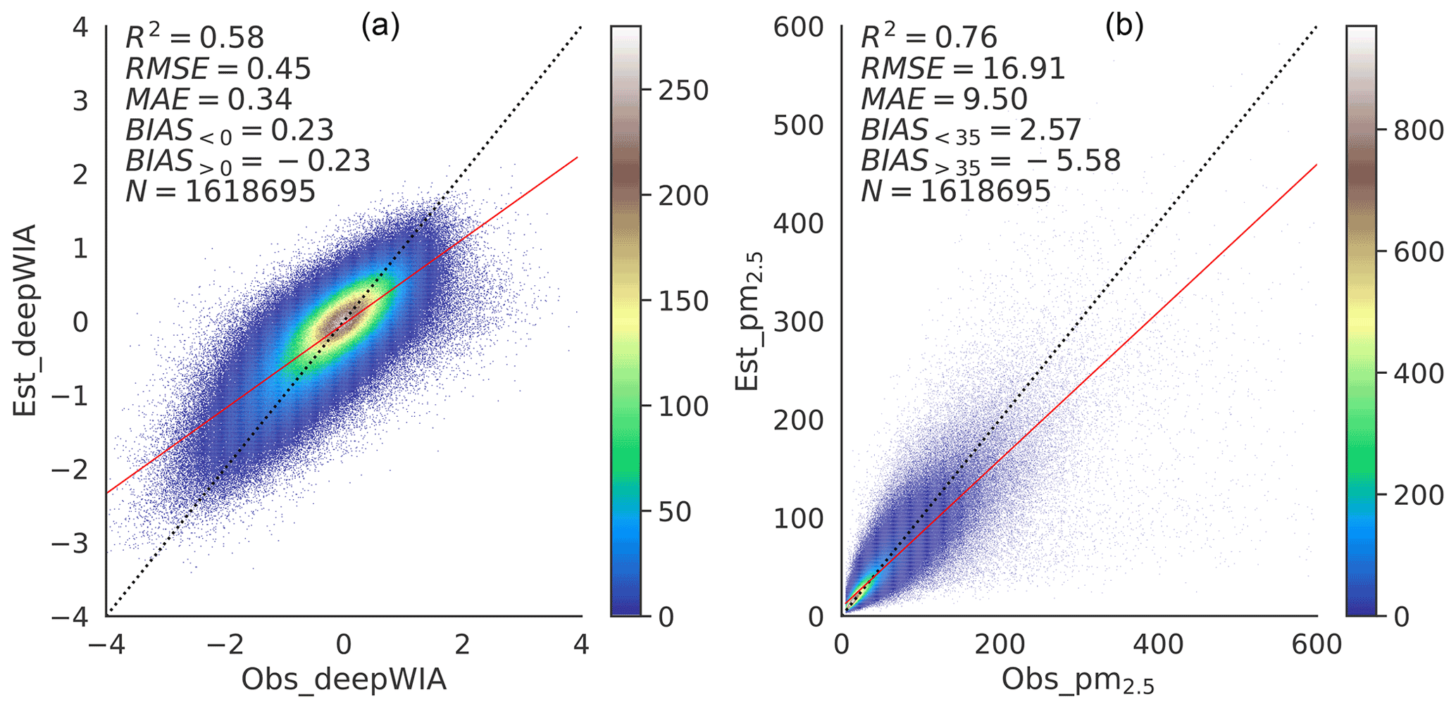
Figure 3 Training density scatterplots of (a) deepWIA ($\widehat{r}$) and (b) PM_2.5 concentrations using data for 2015–2021 as a training set.

Figure 4 As for Fig. 3, but for the first validation dataset.

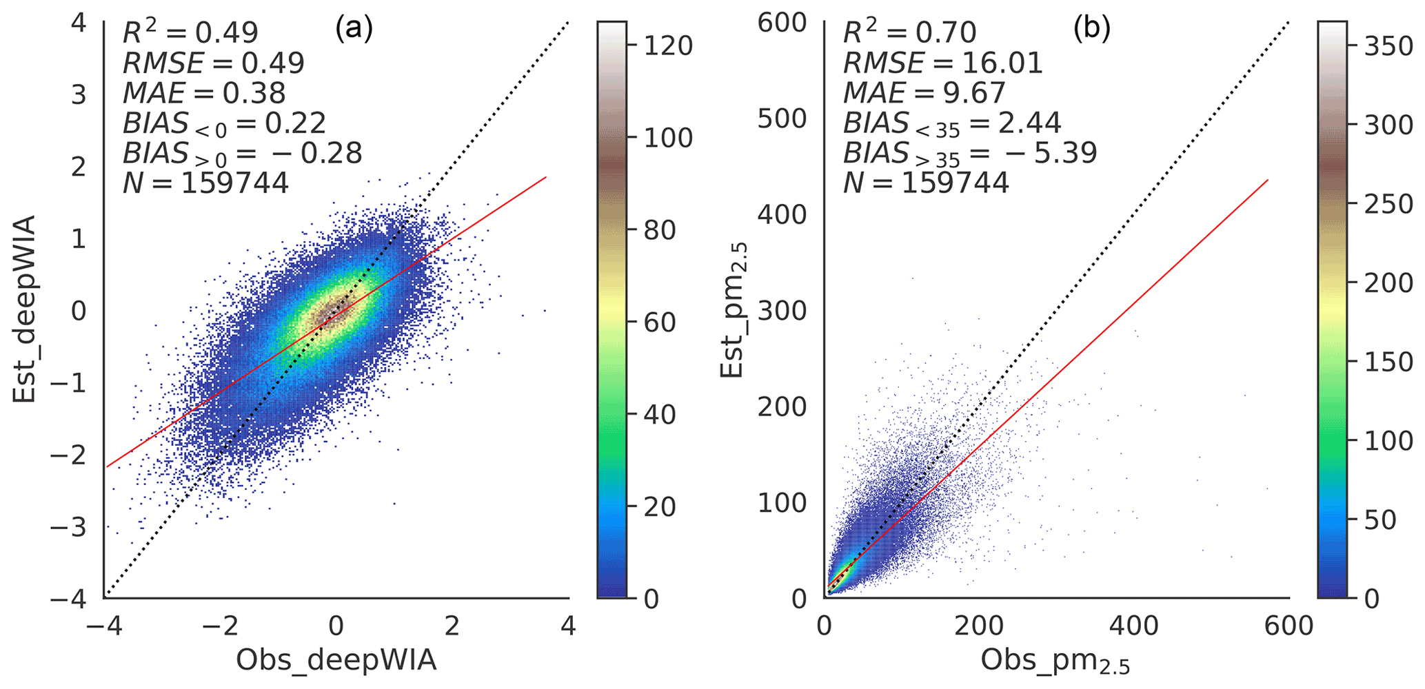
Figure 3 shows the fitting scatterplots of deepWIA and PM_2.5 concentrations for the entire training–validation dataset. The $\widehat{r}$ value had an RMSE of 0.45, an MAE of 0.34, and an R² value of 0.58. The PM_2.5 concentration had an RMSE of 16.91 µg m⁻³, an MAE of 9.5 µg m⁻³, and an R² value of 0.76. Additionally, The DL model still underestimated high values and overestimated low values, although label transformation and some other processes were performed.

Scatterplots for the first validation dataset (Fig. 4) show slightly lower performance than that for the training set (RMSE = 0.49, MAE = 0.38, and R²=0.49 for $\widehat{r}$; and 16.01 µg m⁻³, 9.67 µg m⁻³ and 0.70, respectively, for PM_2.5 concentration), partly because of the smaller set of training samples than that used in final training. Validations in the other nine validation datasets had similar performance, as summarized in Figs. S2 and S3. The RMSE and R² values for $\widehat{r}$ for these validation datasets were in narrow ranges of 0.48–0.55 and 0.47–0.50, and the RMSE and R² values for PM_2.5 concentrations were 0.67–0.77 and 15.54–21.68 µg m⁻³, respectively. These metrics for 10-fold CV indicate no significant overfitting by the final deepWIA model and prove the stability of the model generated by the ResNet–GRU structure.

Once the DL model is established after training, a question worth discussing is the relative importance of these input variables. A DL model cannot answer by voting as the RF model. Therefore, here we perform sensitivity experiments to solve the problem: (1) for every input variable shown in Table 1, we deactivate it by setting all related model parameters to zero in the first convolutional layer; (2) we apply the modified model (i.e., without the effect of the given variable) to the training dataset and compute the RMSE of deepWIA; (3) we compute the difference between the RMSE and that of the original model. The larger the RMSE increases, the more important the input variable is. We applied these steps to all input variables and showed their importance rankings in Table 1. The five most important variables are latitude and longitude, 2 m mixing ratio, population density, maximal 2 m temperature, and surface turbulence stress components. However, some variables take little effect on the model (with an RMSE increase of less than 0.001), including wet deposition potency, precipitation, geopotential height at 850 hPa, ventilation potency, downward short-wave radiation, low cloud cover, and high vegetation cover.

Figure 5 As for Fig. 3, but for the test dataset for 3 January to 30 April 2022.

Nevertheless, it would not be fair to compare the contribution of individual input variables to the DL model because there are overlaps in the contribution of several variables, such as 100 and 10 m winds. Therefore, we grouped all variables into six groups, namely near-surface wind variables, near-surface temperature-humidity variables, near-surface vertical diffusion variables, spatiotemporal geographic variables, synoptic pattern and radiation variables, and precipitation variables (Table S1 in the Supplement). Using the same approach as the individual variable, we compute the importance of each group of variables. The most important group is the spatiotemporal geographic variable, followed by the vertical diffusion and near-surface wind variables. The least important one is precipitation (Fig. S4).

3 Model performance on the test dataset

Data for 3 January to 30 April 2022 were used as the test dataset including about 85 000 samples to demonstrate model performance in the normal aerosol-pollution season in China. Feeding the input variables from the test dataset into the final deepWIA model yields the estimated $\widehat{r}$. A scatterplot of $\widehat{r}$ and the corresponding PM_2.5 concentration of the test dataset is shown in Fig. 5. The $\widehat{r}$ value had an RMSE of 0.5, an MAE of 0.39, and R² of 0.53. The performance just decreased slightly relative to that with the training set, indicating that the deepWIA model is strongly robust with the test dataset. And the $\widehat{r}$-based PM_2.5 concentrations had an RMSE of 16.54 µg m⁻³, an MAE of 10.25 µg m⁻³, and R² of 0.72. Note that some of the evaluation metrics were better than those of validation datasets because more samples were used to generate the final model than were used in validation. The stable performance using the training set, the 10-fold CV sets, and the test dataset indicates that our model can be safely used for quantifying weather conditions of PM_2.5 concentrations, at least in aerosol-pollution seasons.

The geographic distribution of biases and RMSEs for $\widehat{r}$ and PM_2.5 concentrations estimated by the deepWIA model are shown in Fig. 6. There was no significant estimation bias of $\widehat{r}$ with observations in most grid cells. Small overestimations (positive biases) of $\widehat{r}$ occurred in Northeast China, the North China Plain (NCP), Ningxia, and the Zhuhai–Hong Kong–Macao Bay area (ZHM), whereas underestimations (negative biases) mainly occurred in south-central China. The estimated PM_2.5 concentration remained unbiased in some areas but was underestimated in some grid cells in the NCP, Northeast China, the Sichuan Basin, and south-central China, with values of −6 to −8 µg m⁻³. The model also significantly underestimated PM_2.5 concentrations in the area around the Taklamakan Desert by up to −10 µg m⁻³. The $\widehat{r}$ values had small RMSEs in the southern NCP, the Sichuan Basin, and the ZHM, with corresponding small RMSEs in estimated PM_2.5 concentrations of 0–10 µg m⁻³. Larger RMSEs for PM_2.5 concentrations occurred in some grid cells located in Northeast China, Xinjiang, Ningxia, and the western NCP, with values of >20 µg m⁻³. Large RMSEs and biases in Xinjiang and Ningxia may be attributed to the frequent occurrence of dust storms there (Wang et al., 2004). Due to the scarcity of samples, a meteorological data-based model cannot fully understand dust storm occurrence.

Figure 6 Test biases (a, c) and RMSEs (b, d) in deepWIA ($\widehat{r}$) (a, b) and PM_2.5 concentrations (c, d) over China from 3 January to 30 April 2022.

Eight cities were selected to illustrate the performance of the deepWIA model in time series, with analysis of daily variations in PM_2.5 concentrations (Fig. 7). The cities (Fig. 6c) are in northern China (Beijing and Xi'an), eastern China (Shanghai and Hangzhou), southwest China (Chengdu and Chongqing), and south-central China (Wuhan and Changsha), all of which suffer from aerosol pollution.

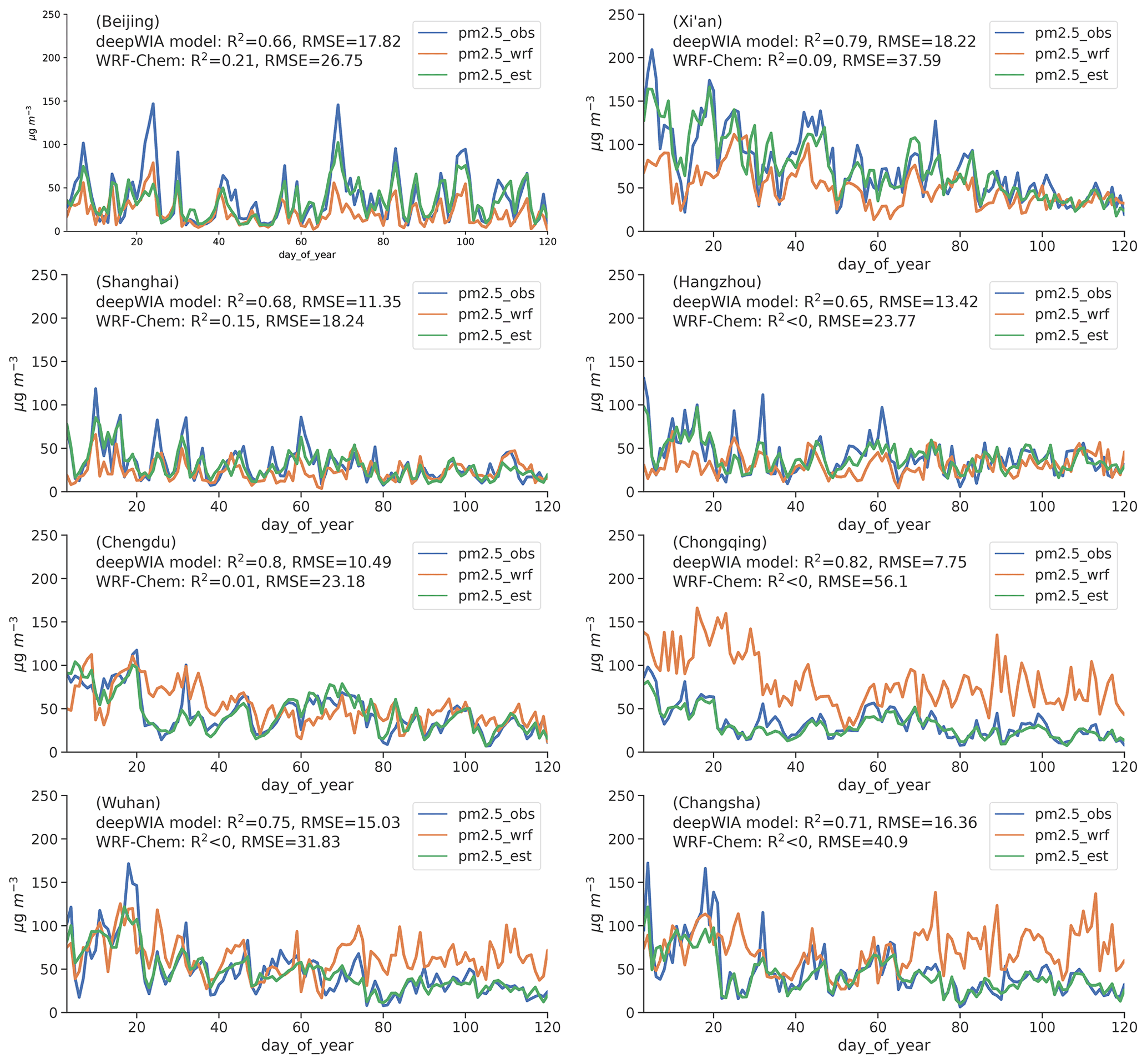
Figure 7 Day-to-day series of PM_2.5 concentrations based on observations (blue curves), WRF-Chem (orange curves), and deepWIA model (green curves) in eight cities in China, 3 January to 30 April 2022.

For comparison, the results of a WRF-Chem simulation are also presented (Fig. 7). Similar to deepWIA, we also use the ERA5 data to drive the WRF-Chem model. Hence, both WRF-Chem and deepWIA models are run in hindcast mode. The simulation domain covered China, including the above eight cities, with a high horizontal resolution of 9 km. The model used the Multi-resolution Emission Inventory for China (MEIC, http://meicmodel.org/, last access: 3 August 2022) (Li et al., 2017) as an emission inventory. To avoid weather-system drift due to long-term model integration (Feng et al., 2020a), the simulation restarted every day at 12:00 UTC, with the mean of 12–35 h (i.e., 00:00–23:00 UTC) simulated PM_2.5 concentrations being used as the daily value.

Estimations using the deepWIA model captured day-to-day variations in PM_2.5 concentrations, outperforming the WRF-Chem simulation in all eight cities with a significant reduction in RMSEs and improvement in R² (RMSEs ≤ 19 µg m⁻³ and R²≥0.65). The simulation accuracy of WRF-Chem varied substantially in different regions of China. The four cities, including Beijing, Shanghai, Hangzhou, and Chengdu, yielded good performances, with RMSE ≤ 30 µg m⁻³. The WRF-Chem model largely failed to capture the day-to-day variations in aerosol concentrations in the other five cities. In comparison, the deepWIA model gave a robust performance in both northern and southern China, indicating a wide application potential for different regions. In conclusion, Fig. 5 shows that the main problem with the deepWIA model is underestimation in extreme values of PM_2.5 concentration, leading to the omission of some heavy haze events.

To further present the good performance of the deepWIA model, two additional comparisons with WRF-Chem are given. The first is the comparison of synoptic variabilities that remove the variation longer than 31 d (Fig. S5), like the timescale focused by the deepWIA model. The second is a comparison with an operational system for air quality forecast based on WRF-Chem (Fig. S6). The simulation has the same spatial and temporal resolution as the ERA5-driven one above but is optimized for northern China. To reduce initial and boundary errors, the system used the real-time assimilated meteorological field and assimilated PM_2.5, PM₁₀, SO₂, NO₂, O₃, and CO concentrations within the domain using the newly developed 3DVar module for WRF-Chem. In both comparisons, the deepWIA model significantly outperforms the corresponding WRF-Chem simulations for all eight cities.

4 Ablation experiments and related studies

4.1 Comparison of ablation experiments

Although the deepWIA appears accurate and robust in capturing synoptic variations in PM_2.5 concentrations, it is of interest to investigate the reason for its strong performance. The model has three key points: (1) a ResNet–GRU structure with more meteorological variables; (2) a timescale separation approach making the model focus only on the effects of meteorology on synoptic variations in PM_2.5 concentrations; and (3) a label transformation approach based on a logarithmic function to mitigate data imbalance. To investigate the relative importance of these processes for the final deepWIA model, two additional ablation experiments were performed for comparison:

• AbExp_1: with fitting of PM_2.5 concentrations directly using the same ResNet–GRU structure, samples, and training strategy, but with no timescale separation or label transformation. This experiment was similar to studies of ML-based PM_2.5 concentration retrieval but using meteorological variables as primary data. This experiment was intended to assess the basic fitting power due to the DL structure and input variables.

• AbExp_2: with fitting of r (Sect. 2.2) using the same model structure, samples, training strategy, and timescale separation, but with no label transformation. A comparison of the results of AbExp_1 and AbExp_2 illustrates the importance of timescale separation. A comparison of the results of AbExp_2 and original deepWIA illustrates the impacts of label transform.

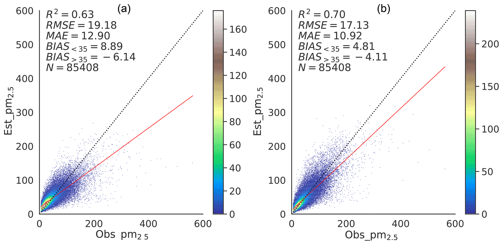
Figure 8 Density scatterplots of PM_2.5 concentrations for the test dataset from the ablation experiments (a) directly using the PM_2.5concentration as the target, and (b) using r as the target (i.e., without label transform based on logarithmic function).

Scatterplots of PM_2.5 concentrations for AbExp_1 and AbExp_2 using the same test dataset as that used for the deepWIA model are shown in Fig. 8. The AbExp_1 experiment had an RMSE of 19.18 µg m⁻³, an MAE of 12.9 µg m⁻³, and an R² value of 0.63, achieving the level of ML-based PM_2.5 concentration retrieval (Sect. 4.2). The DL structure and the feature engineering for input variables thus builds a solid foundation for the fitting power of the deepWIA model. Compared with AbExp_1, AbExp_2 improved the R² value to 0.70, with the RMSE decreasing to 17.13 µg m⁻³ and the MAE to 10.92 µg m⁻³, indicating the importance of timescale separation. Furthermore, the focus on synoptic variation also helped mitigate the overestimation of low values and underestimation of high values. The final deepWIA model further improved the general performance in estimating PM_2.5 concentrations, with improved R², MAE, and RMSE values. The logarithmic function-based label transformation mitigated the overestimation of low values while exacerbating the underestimation of high values, with this treatment increasing the distance between low values but decreasing the distance between high values of the samples. A scheme such as AbExp_2 may therefore be applicable to studies of extreme haze events. To summarize, model and feature engineering are most important in determining the final performance of the deepWIA model, with timescale separation and label transformation following in that order.

4.2 Comparison with models used in previous studies

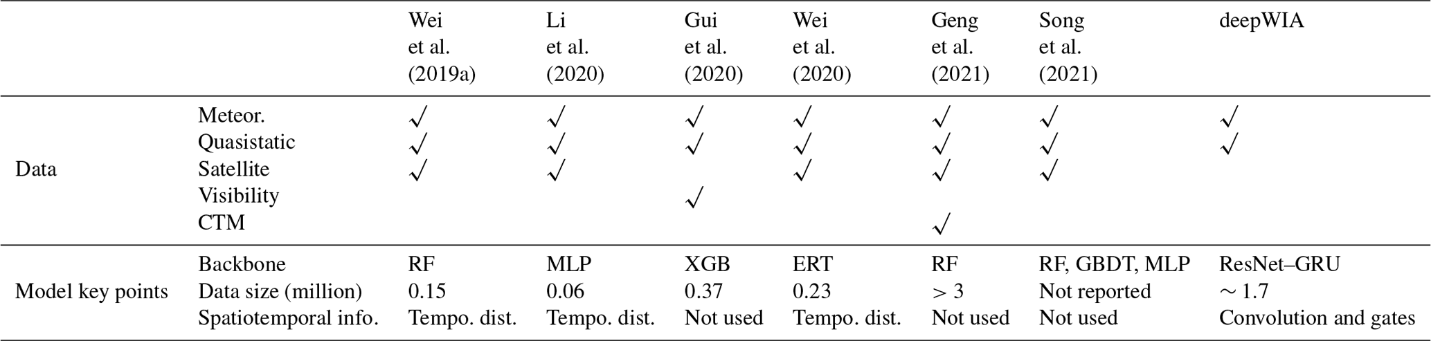
Recent studies of PM_2.5 concentration retrieval use ML/DL models such as RF, XGB and MLP (Table 2). Unlike our model, these studies were not concerned with the role of meteorology but only with the accuracy of estimated PM_2.5 concentrations. There are many differences between these methods and the deepWIA model in the model-building processes. For example, (1) the deepWIA model uses timescale separation to focus on synoptic variations in aerosol concentrations caused by meteorology. We do not use an emission inventory as an input feature for the model because of its significant uncertainty. It is difficult for DL models, which rely heavily on input data, to build robust relationships among emissions, meteorology, and aerosol concentrations. (2) Except for the approach of Geng et al. (2021), the training sample size used in deepWIA is much larger than that used in previous models, which often used data of 1 year for training (Geng et al., 2021 also built the ML model year-by-year, starting from 2013). The large sample size aids the building of a more robust model. (3) We introduce more derived meteorological variables than most studies by feature engineering.

Table 2 Comparison of studies of observation retrieval of PM_2.5 concentrations and deepWIA. “√” indicates data used as model input features. ERT and GBDT denote extreme random trees and gradient boosting decision trees, respectively.

Therefore, to make a fair comparison of the model per se, we use six popular ML/DL models, with the same periods, stations, and input parameters as the deepWIA model, including two RF, two XGB, and two MLP models using the input data over 3 d (i.e., the same as the deepWIA) and only 1 d that is fitted, named RF1, RF3, XGB1, XGB3, MLP1, and MLP3 respectively (Table 3). The MLP models have nine full connection layers with the maximal 512 neurons in the fifth layer. Following the previous studies, all the models fit the PM_2.5 concentrations directly. It should be noted that these models are applied here for the role of meteorological variables and thereby do not introduce satellite or visibility data, so the RMSEs here are slightly higher than those reported in previous studies.

Table 3 Comparison of ML/DL models performance using the same time periods, stations, and input parameters as the deepWIA model.

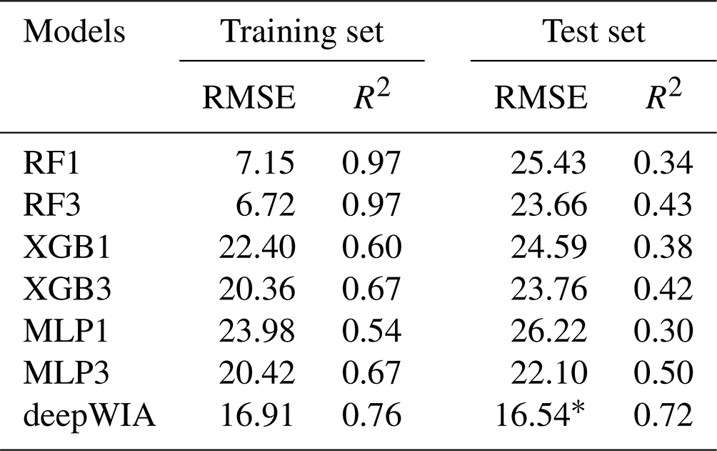
^* Note that the RMSE of deepWIA on the test dataset is smaller than that on the training dataset because the model does not directly fit the PM_2.5 concentration.

These six models all have higher RMSEs and lower R² than the deepWIA model in the test set (even than that of the AbExp_1, which also fits PM_2.5 concentrations directly; Fig. 8a). The models with 3 d data always performed better than these with only 1 d data, indicating the importance of temporal information. Additionally, there is more severe overfitting for these models than the deepWIA model, as evidenced by the large performance difference between the training and test sets, especially those of the RF1 and RF3.

The advantages of deepWIA over traditional RF, XGB and MLP models should be attributed to two points: (1) the deepWIA model is much deeper than the commonly used RF, XGB and MLP models, which aids learning of the complex nonlinear relationship between meteorology and aerosol concentration; and (2) previous models do not necessarily include temporal correlations of aerosol concentrations; rather, some use a predefined spatiotemporal distance for the injection of temporal information (Wei et al., 2019a, b, 2020; Li et al., 2020). The deepWIA model uses gate parameters to learn dynamic links of aerosol concentration among days.

We also compare the deepWIA and two semiempirical meteorological indices for aerosol pollution, namely PLAM and ASI. These indices are commonly used to assess meteorological effects on variations in aerosol concentrations (Wang et al., 2021; X. Zhang et al., 2019). PLAM was applied to the NCP (Yang et al., 2016), using visibility as the target variable, while ASI was applied to North and Northeast China, using PM_2.5 concentrations as the target variable. Both indices only considered the meteorology on that day only. By comparison, as described in Section 2.1, deepWIA includes all the kernel variables of these two indices, as well as other spatiotemporal information. It will form the best DL model to take advantage of these variables. Hence, its applicability extends to the whole country. Additionally, PLAM and ASI cannot provide a uniform model for PM_2.5 concentrations, unlike deepWIA. PLAM focused on the relationship between meteorology and visibility; ASI just illustrates the temporal relationship between meteorology and PM_2.5 concentrations, which varies from location to location. Therefore, estimating PM_2.5 concentrations also requires additional linear modeling at each grid cell. Due to these advantages, the deepWIA could be a better tool for assessing the impact of weather on aerosol concentrations.

5 Spatial distribution of deepWIA and its application in quantifying the aerosol-related weather condition

This section is to show the geographic distribution of deepWIA ($\widehat{r}$) over the test period, which can also be used to quantify the aerosol-related weather conditions over China. A positive or negative deepWIA indicates weather-related enhancement or reduction of aerosol pollution, respectively, relative to background concentrations (B). We prepared an animation of daily deepWIA from 3 January to 30 April 2022, to illustrate synoptic variations in aerosol-associated weather in China (see the data availability statements). To assess weather conditions over the test period, we applied a statistical metric, the ratio of good weather (RGW) days for aerosol pollution calculated as

$$\begin{array}{}\text{(4)}& \mathrm{RGW}=N_{\widehat{r}\le \mathrm{0}}/N,\end{array}$$

where $N_{\widehat{r}\le \mathrm{0}}$ and N denote the number of days with $\widehat{r}\le \mathrm{0}$ values and total days over the test period, respectively.

The geographic distributions of the RGW indicate that most areas in China had good weather for higher air quality during January–April 2022 (Fig. 9). In south-central China, almost all grid points had RGWs > 0.5 and negative MVs, implying favorable weather conditions for higher air quality. In Beijing, RGW was about 0.65, implying a 15 % increase in clean air days relative to background concentrations. Unfavorable weather for aerosol pollution was found mainly in the south-central NCP and on the western fringe of the Sichuan Basin, with RGWs of 0.4–0.5. Note that with Eqs. (1) and (2), all synoptic-scale changes are relative to long-term background concentrations for the same season of the last two years. A similar approach can be used to compare the effects of weather on aerosols between two periods (e.g., 2 years), by replacing the background concentration with that calculated over the base period.

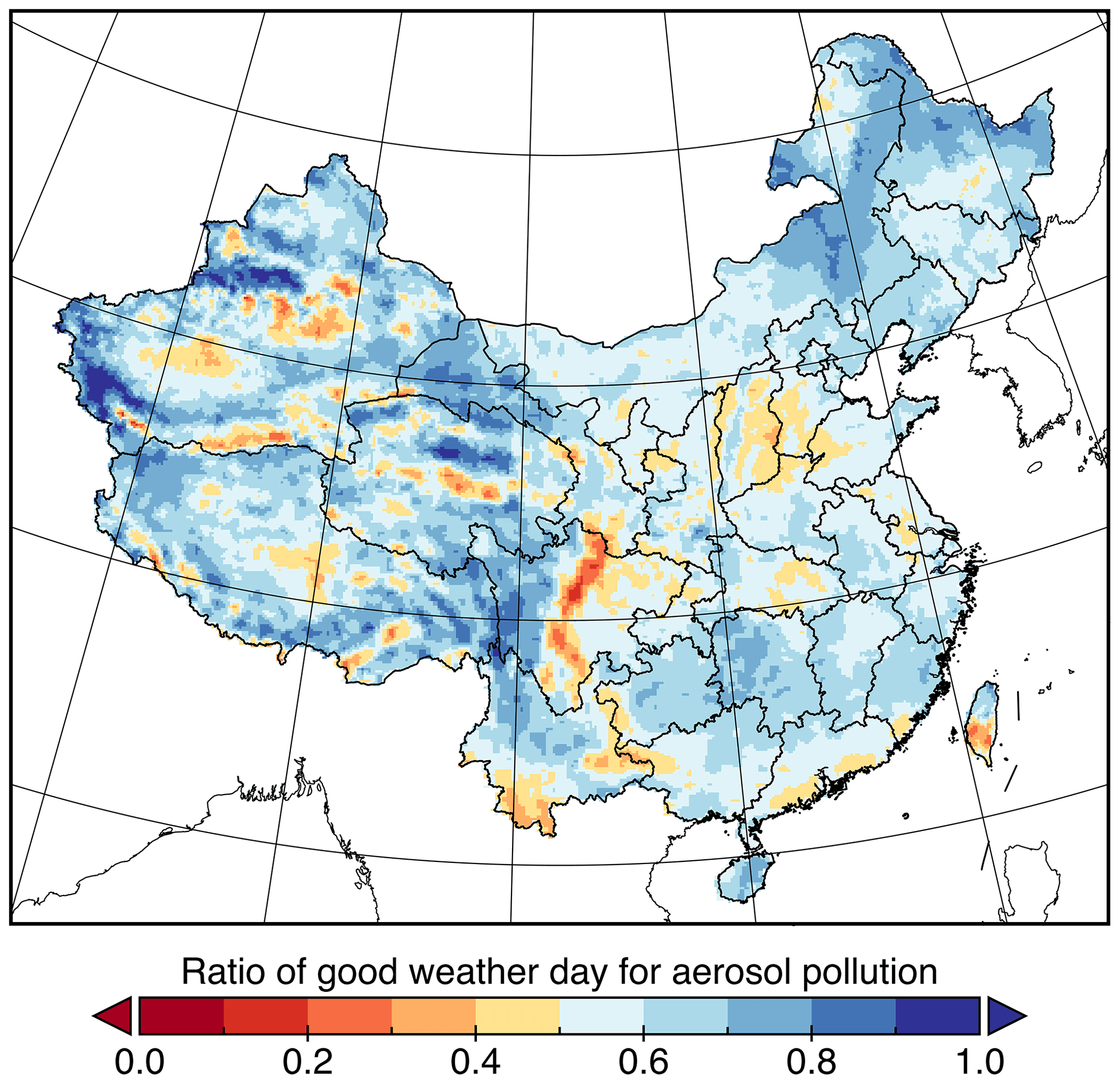
Figure 9 Geographic distributions of the ratio of good weather (RGW) days for PM_2.5 concentrations, 3 January to 30 April 2020.

6 Conclusions

We propose a spatiotemporal deep network architecture to link meteorology and aerosol concentrations. The network uses a 49-layer ResNet structure to extract meteorological information in the vicinity of observed grid points and a GRU to dynamically fuse the information from the ResNet for 3 consecutive days. Many approaches were undertaken in improving its performance, including feature engineering, timescale separation, and logarithmic function-based label transformation. Based on the model, we produced a meteorology index, deepWIA, to capture synoptic variations in aerosol concentrations.

The model was trained and 10-fold CV applied using ground-based PM_2.5 observations in China and ERA5 meteorological fields for the period 2015–2021. Tests were performed using data for January–April 2022. The results indicate that the model well estimates synoptic variations in PM_2.5 concentrations and corresponding weather changes. Performance using the test dataset does not decrease significantly relative to the training set, indicating very weak overfitting in the model. We also compared time series of PM_2.5 concentrations between deepWIA and WRF-Chem in eight cities in China. The deepWIA performed better than WRF-Chem simulations with higher R² values and lower RMSEs in each city. In particular, the model yields consistent simulating power in both southern and northern China, whereas WRF-Chem failed to capture aerosol variations in four cities in southern China. The predictive power of the deepWIA model also outperformed the previously reported PM_2.5 concentration retrieval scheme based on other ML/DL models.

The strong performance of deepWIA is due to the powerful ResNet–GRU architecture and the treatment of timescale separation. Meteorology and emissions dominate different timescales in aerosol variations. Meteorological variables also vary on different timescales, ranging from hourly to interannually. Therefore, it is very difficult to accurately estimate aerosol concentrations directly using a single data-based model. The timescale separation used in this study is thus necessary in allowing the model, despite its complexity, to focus on day-to-day variations in aerosol concentrations and associated weather.

As the background aerosol concentration is currently computed from observations, the deepWIA model cannot directly provide the spatial distribution of aerosol concentrations. However, this can be obtained from a CTM simulation, observation retrieval, or even another ML/DL learning model. Owing to the strong performance of deepWIA, a study is planned for short- and medium-range forecast schemes for PM_2.5 concentrations based on the spatiotemporal DL model and numerical weather prediction (NWP). In a real medium-range forecast system, a re-trained deepWIA model should be applied, with the real-time NWP data (i.e., from ECMWF or WRF) as input meteorological data. Moreover, a short-range forecast DL model should be more complex as it is more sensitive to initial aerosol concentrations. Therefore, more variables such as pre-forecast observations should be injected into the DL model to provide better initial conditions.