the Creative Commons Attribution 4.0 License.
the Creative Commons Attribution 4.0 License.
 | 10 Mar 2023
South Pole Station ozonesondes: variability and trends in the springtime Antarctic ozone hole 1986–2021
Bryan J. Johnson
Patrick Cullis
John Booth
Irina Petropavlovskikh
Glen McConville
Birgit Hassler
Gary A. Morris
Chance Sterling
Samuel Oltmans
Balloon-borne ozonesondes launched weekly from South Pole Station (1986–2021) measure high-vertical-resolution profiles of ozone and temperature from the surface to 30–35 km altitude. The launch frequency is increased in late winter before the onset of rapid stratospheric ozone loss in September. Ozone hole metrics show that the yearly total column ozone and 14–21 km partial column ozone minimum values and September loss rate trends have been improving (less severe) since 2001. The 36-year record also shows interannual variability, especially in recent years (2019–2021). Here we show additional details of these 3 years by comparing annual minimum profiles observed on the date when the lowest integrated total column ozone occurs. We also compare the July–December time series of the 14–21 km partial column ozone values to the 36-year median with percentile intervals. The 2019 anomalous vortex breakdown showed stratospheric temperatures began warming in early September followed by reduced ozone loss. The minimum total column ozone of 180 Dobson units (DU) was observed on 24 September. This was followed by two stable and cold polar vortex years during 2020 and 2021 with total column ozone minimums at 104 DU (1 October) and 102 DU (7 October), respectively. These years also showed broad near-zero-ozone (loss saturation) regions within the 14–21 km layer by the end of September which persisted into October.
Validation of the ozonesonde observations is conducted through the ongoing comparison of total column ozone measurements with the South Pole ground-based Dobson spectrophotometer. The ozonesondes show a more positive bias of 2 ± 3 % (higher) than the Dobson following a thorough evaluation and homogenization of the long-term ozonesonde record completed in 2018.
- Article
(7181 KB) - Full-text XML
- BibTeX
- EndNote


In 1986, NOAA began launching weekly balloon-borne ozonesondes at Amundsen–Scott South Pole Station (90∘ S) measuring high-resolution vertical profiles of ozone and temperature. This same year numerous field projects were deployed to Antarctica (Anderson et al., 1989; Tuck et al., 1989) to investigate the discovery of the springtime Antarctic ozone hole by Farman et al. (1985). Subsequent studies confirmed that the chlorine catalytic destruction of ozone was enhanced over Antarctica in the presence of wintertime polar stratospheric clouds (PSCs) (Solomon, 1999; Solomon et al., 1986; McElroy et al., 1986). The following decade of balloon-borne profiles and satellite and ground-based measurements showed a broad and deepening ozone hole that stabilized in its expansion by the early 2000s (Hofmann et al., 2009). More recently, several analyses of the ongoing ground-based and satellite measurements indicate that the ozone hole has been slowly recovering since 2000 (for a list of studies, see Langematz et al. (2018). The current recovery stage and upward trend in springtime ozone have been linked to the decline in the concentration of man-made ozone-depleting substances (ODSs) due to the successful implementation of the Montreal Protocol international guidelines phasing out the production of ODSs. In 2020, the ODS abundance over Antarctica was 25 % below the 2001 peak (Montzka et al., 2021). Full recovery is predicted to occur by around 2056–2070 when ODS levels return to the 1980 benchmark levels (Newman et al., 2006; Dhomse et al., 2018; Amos et al., 2020). However, while long-lived ODS concentrations are steadily declining, the extent of chemical ozone loss may be quite different from year to year due to meteorological conditions (Newman et al., 2006; Keeble et al., 2014; de Laat et al., 2017; Tully et al., 2019; Stone et al., 2021).
After polar sunset, the strengthening of circumpolar winds and the development of a potential vorticity gradient form the polar vortex boundary region that isolates stratospheric air over Antarctica (Nash et al., 1996). Near the center of the vortex, over the South Pole, ozonesondes measure stratospheric temperatures steadily decreasing during the polar night and remaining well below the −78 ∘C threshold for PSC formation and growth. PSCs provide the surface reaction sites for activating stable chlorine species into radicals that rapidly destroy ozone after sunlight returns in September (WMO, 2018). However, planetary wave disturbances in late winter may weaken or completely break apart the cold and stable Antarctic polar vortex, ending the optimum conditions for rapid ozone loss in September (Schoeberl et al., 1989; Newman et al., 2004; Hassler et al., 2011a; Salby et al., 2012; Strahan et al., 2016; de Laat et al., 2017; Strahan et al., 2019; Milinevsky et al., 2020). These conditions were observed in the warmer and weaker polar vortex conditions in 1986 and 1988 (Stolarski et al., 1990). The most extreme disruptions in the polar vortex occurred during the stratospheric warming events in 2002 and 2019 (Hoppel et al., 2003; Safieddine et al., 2020; Wargan et al., 2020).
The South Pole ozonesondes play a key role in monitoring ozone and temperature during all phases of the ozone hole. These unique measurements are critical after Antarctic sunset when several months of darkness limit the ground-based Dobson spectrophotometer and solar ultraviolet satellite optical measurements. Several indices and indicators have been presented in past analyses of the Antarctic ozonesonde records by Hofmann et al. (1997, 2009); Solomon et al. (2005, 2016); and Hassler et al. (2011a).
This paper is a review of the South Pole ozonesonde observations beginning with an overview in Sect. 2 of the electrochemical concentration (ECC) ozonesonde and recent homogenization of the South Pole data record by Sterling et al. (2018). Section 3 shows a comparison of ozone and temperature profiles during the last 3 years when the early polar vortex breakup and weak ozone hole in September 2019 were followed by severe ozone loss in 2020 and 2021 when cold vortex conditions persisted into early December (Kramarova et al., 2021, 2022). Section 4 shows the updated 36-year homogenized ozone time series and ozone hole metrics focusing on the 14–21 km layer column ozone minimums and linear ozone loss rates during September. In addition, we update ozone mixing ratio loss rates at selected pressure levels from the analysis by Hassler et al. (2011a) that showed maximum September loss rates occur in the 33–48 hPa region, while the 89 hPa was found to be the optimum layer for observing early detection of reduced ozone loss rates as ODSs decline. Section 5 illustrates the extent of ozone loss saturation observed each year during the annual minimum-ozone period from 26 September to 15 October. The near-zero-ozone layers were variable and narrowing after 2008 but were near maximum extent again in 2020 and 2021. The summary is given in Sect. 6.
The basic design of the electrochemical concentration cell (ECC) ozonesonde has remained relatively unchanged during the 36-year South Pole record (Komhyr, 1967). A Teflon piston pump bubbles ambient air into a sensor cell chamber with a platinum gauze electrode submerged in 3 mL of dilute, buffered potassium iodide (KI) solution. The ozone–iodide reaction in the ECC cell generates an electrical signal proportional to the ozone concentration.
Since about the mid-1990s, the ECC sonde manufacturers have improved the sensor cell design and the purity of the platinum electrodes, thus reducing the sensor's current background to approximately 0.02 µA when sampling no-ozone filtered air (Vömel and Diaz, 2010; Smit and Thompson, 2021). The limit of detection (LOD) is equivalent to 3×0.02 µA background. This converts to an ozone partial pressure of 0.10 mPa or a mixing ratio of 0.02 ppmv (parts per million by volume) at 50 hPa ambient pressure.
A Styrofoam box houses and insulates the ozonesonde pump and sensor. The weather radiosonde, attached to the outside of the box, measures and transmits meteorological and ozone data to the ground-based receiving equipment during ascent to the balloon-burst altitude of about 34 km. Consistent burst altitudes are maintained during the dark, cold months at the South Pole by switching from standard rubber weather balloons to 500 m3 volume polyethylene film balloons during the first week of April and then returning to rubber balloons by mid-October.
2.1 Data homogenization
Each ECC ozonesonde profile represents a new instrument, used only once; thus, ozonesonde trends may show an offset or sudden bias rather than a slow drift in the data record when a new ozonesonde design or standard operating procedure change occurs (Johnson et al., 2002; Smit et al., 2007; Tarasick et al., 2016; Thompson et al., 2017; Van Malderen et al., 2016; Witte et al., 2017). The ozonesonde model and standard operating procedures (SOPs) at the South Pole have not changed since 2006. However, prior to 2006, several dual and triple ozonesondes were flown to compare new ozonesonde models or adjustments made in the SOP in order to determine ad hoc corrections to account for these changes.
A thorough review and homogenization of the ozonesonde record was completed by Sterling et al. (2018) following homogenization methods that were formulated from the Assessments of Standard Operating Procedures (ASOPOS) workshops (Smit and ASOPOS, 2012; Deshler et al., 2017). The ozonesonde guidelines, presented in the ASOPOS GAW/WMO report no. 268 (2021), are based on the World Calibration Center Jülich Ozonesonde Intercomparison Experiments (JOSIE). The JOSIE environmental simulation chamber experiments are the global reference for evaluation of new ozonesonde designs and SOPs and the foundation for improving long-term vertical ozone trends determined by ozonesondes with a goal to reduce uncertainty to ±5 % throughout the profile (Smit et al., 2007; Thompson et al., 2019).
Additional verification of the ozonesonde record at South Pole Station is conducted through the ongoing comparison of total column ozone (TCO) with the NOAA ground-based Dobson spectrophotometer direct-sun (DS) AD wavelength pair measurements over South Pole Station from 20 October to 20 February (Komhyr et al., 1997). Globally, the Dobson network is an important long-term stable reference for ozonesonde sites and useful for identifying drifts in satellite platforms (McPeters and Komhyr, 1991; Bodeker et al., 2005; Thompson et al., 2017). Figure 1 shows the homogenized ozonesonde TCO record is a constant 2 ± 3 % offset compared to the Dobson observations. The Dobson DS/AD observations are accurate to within ±1 % (Köhler et al., 2018). The ozonesonde TCO includes a residual value to account for estimated ozone above the balloon-burst altitude by extrapolating a constant mixing ratio (CMR) from the balloon-burst pressure (occurring between 20 to 7 hPa) to zero pressure. While using the ozone residual lookup values from the satellite SBUV (Solar Backscatter Ultraviolet Radiometer) global climatological residual table from McPeters et al. (1997) and McPeters and Labow (2012) is the recommended procedure for determining ozonesonde residuals (Smit and Thompson, 2021), we have found that the CMR extrapolation is more consistent when comparing with the Dobson spectrophotometer TCO at South Pole Station.
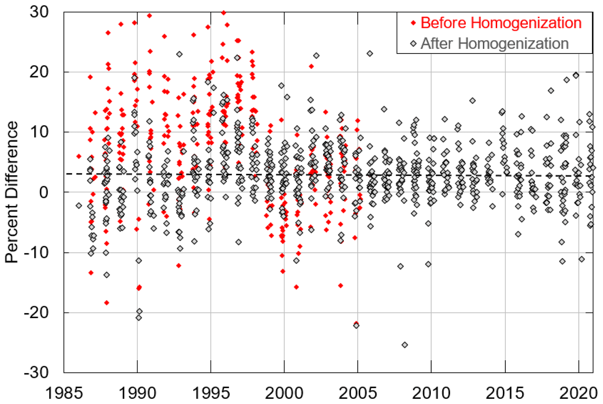
Figure 1Percent difference (100×(sonde − Dobson) Dobson) comparing total column ozone of the South Pole ozonesondes and Dobson spectrophotometer direct-sun AD wavelength measurements. The solid red diamonds represent the percent differences before the homogenization of the 1986–2006 ozonesonde data. The gray diamonds show a more consistent record after homogenization. The dashed horizonal line shows the trend in the offset is relatively stable at 2 %.
2.2 Temperature profile validation
Sterling et al. (2018) discuss the details in the transition from three different radiosonde models at the South Pole from VIZ (1986–1991) to Vaisala RS80 (1991–2014) and the current GPS-enabled InterMet (Imet) radiosondes (2015–2021). The Imet measurements added GPS-computed winds and geometric altitude to the South Pole profile data. For homogenization of the non-GPS Vaisala RS80 data, the NOAA SkySonde software (Allen Jordan author – see acknowledgements) was updated to retrieve nearby weather service radiosonde data. This provided a data source to identify and flag temperature outliers and to adjust the radiosonde pressure when offsets were >2 hPa near burst altitude (Sterling et al., 2018).
The ozonesonde radiosonde temperatures were not adjusted in the homogenization of the data record. However, temperature accuracy for each flight was validated by comparing it with an additional radiosonde flown by the Antarctic Meteorological Research Center (AMRC) at the South Pole. For nearly a decade, the AMRC–South Pole Meteorology Office radiosondes (using Vaisala RS92 and Vaisala RS41 GPS models) were “piggy-backed” on board the NOAA ozonesonde package. This is an important collaboration during the winter months when NOAA switches to the cold-resistant polyethylene balloons to maintain burst altitudes of 30–34 km. This results in two independent temperature profiles to monitor the coldest temperatures in the polar stratosphere where PSCs begin to form. The typical rubber balloon will fail/burst at 14–15 km over the South Pole under these extreme cold and dark conditions. The comparisons between the Vaisala radiosonde models (RS80 and RS92) during the 2012–2013 flights show almost no difference in stratospheric temperature measurement during the summer months and only a slight 0.2 ∘C difference in winter. The Imet radiosonde measures slightly higher temperatures by about 0.5 ∘C than the Vaisala RS41, primarily during the summer months. Steinbrecht et al. (2008) observed similar offsets in campaigns comparing Vaisala RS80 and RS92 radiosondes.
Balloon-borne ozonesondes provide a unique overview of the yearly ozone hole over the South Pole by comparing vertical profiles measured during winter (before depletion begins) with the annual minimum-ozone profile typically observed between 26 September to 15 October. Figure 2 shows the 2019–2021 ozone (upper panels) and temperature (lower panels) profiles representing the ozone holes of these 3 years. The winter profiles (blue) are an average of the six to eight vertical profiles measured from 15 June to 15 August, when the stratospheric temperatures range between −85 to −95 ∘C and TCO averages 263 ± 17 Dobson units (DU).
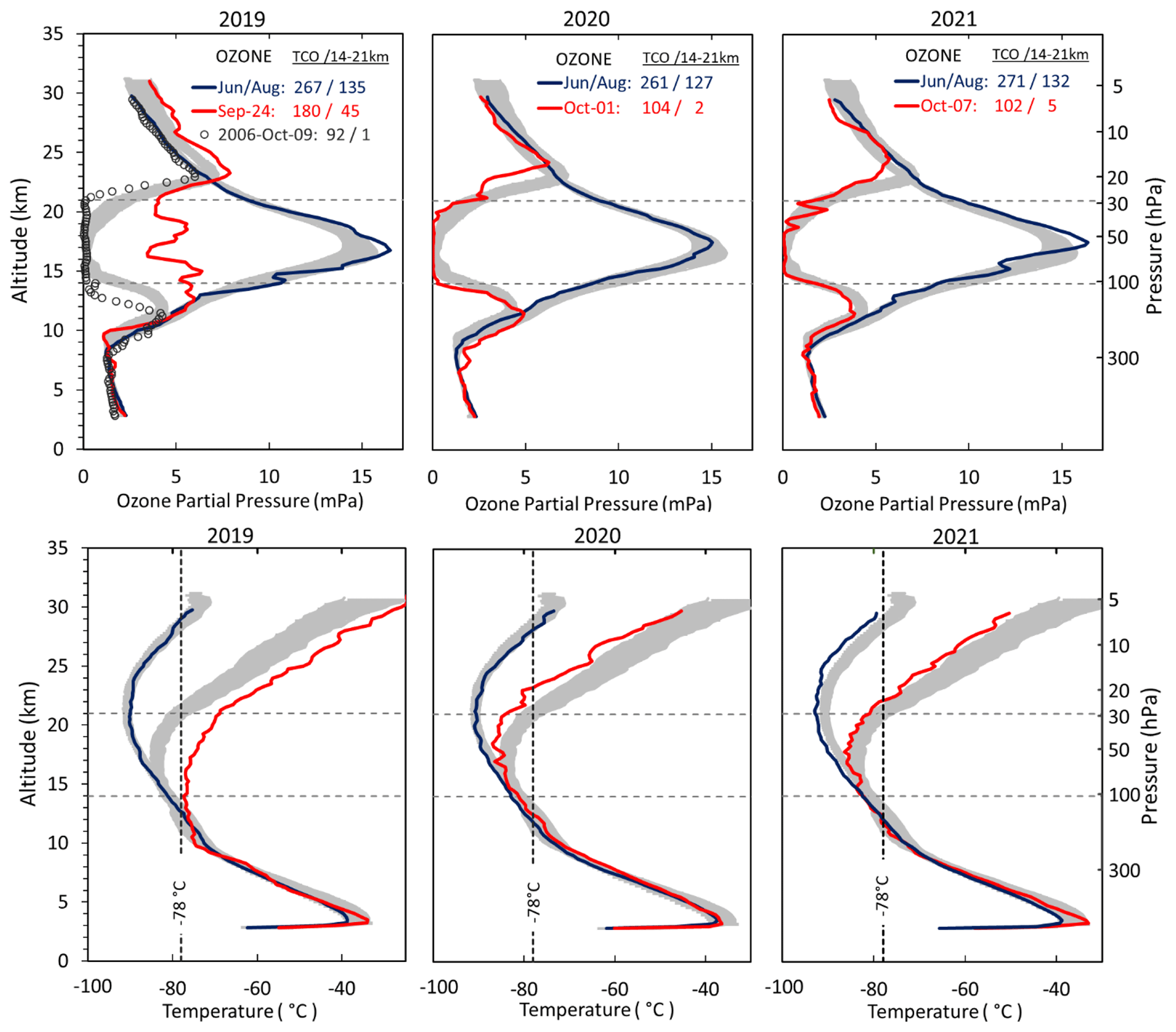
Figure 2Selected ozonesonde profiles from 2019–2021 representing the ozone hole severity over the South Pole by comparing the average winter profile before depletion begins (blue line) to the minimum-ozone profile (red line). The minimum total column ozone (TCO) and 14–21 km (dashed horizontal line region) partial column ozone values are given in Dobson units (DU). The gray shaded region represents the 1986–2018 median 30–70th percentiles for winter and minimum periods. The record low of 92 DU TCO measured in 2006 is shown as a dotted line in the 2019 graph. The temperature graphs show the −78 ∘C PSC threshold as a dashed vertical line.
The wintertime ozone profiles are similar to the long-term climatology each year and typically do not provide any insight into how the polar vortex conditions and the severity of ozone depletion will unfold when rapid depletion begins by 1 September at the South Pole. However, during the last 2 weeks of August the first signs of ozone loss are occasionally observed above 21 km, likely from transported air parcels originating near the polar vortex boundaries where sunrise, Cl2 photolysis, and chemical ozone destruction begin (Schoeberl and Hartmann, 1991; Lee et al., 2001; Hassler et al., 2011a; Strahan et al., 2019).
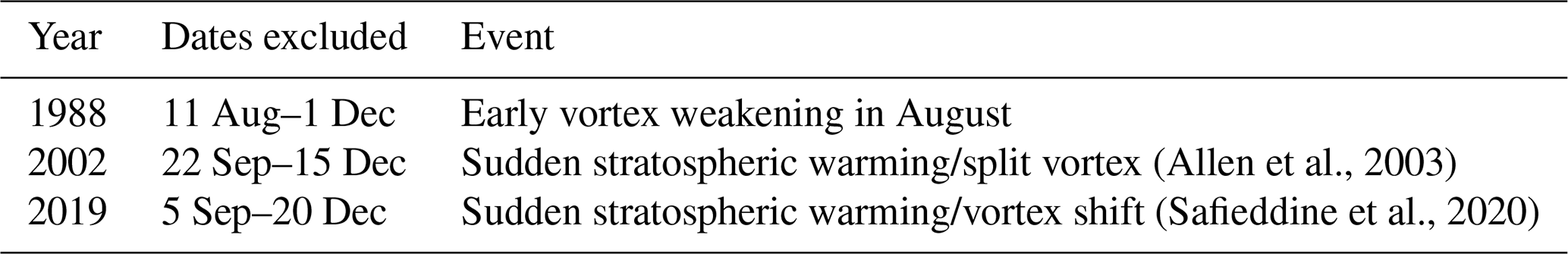
The springtime minimum-TCO profiles (red) average 114 ± 15 Dobson units (DU), which represents a 55 %–65 % ozone loss when compared to the wintertime profile. The 2019 minimum TCO of 180 DU was observed on 24 September, the second-highest minimum in the 36-year South Pole record. This was the third season when the polar vortex was dramatically disrupted, leading to an early September warming and meridional mixing of ozone-rich air into the polar region from the mid-latitude stratosphere (Wargan et al., 2020; Safieddine et al., 2020). Table 1 lists the other 2 years (1988 and 2002) when similar events occurred. The table also includes the date intervals when data were excluded in our long-term median calculations since these extremes in ozone and temperatures were not representative of typical chemical ozone hole losses.
Table 1Years when an early disruption of the polar vortex was observed over the South Pole and the corresponding period when the profile data were excluded from the ozonesonde median and percentile climatology.
The stable and cold polar vortex conditions in 2020 and 2021 led to severe ozone holes over the South Pole with minimum-TCO measurements of 104 DU on 1 October and 102 DU on 7 October, respectively. The profiles in Fig. 2 show the near-complete destruction of ozone within the 14–21 km vertical layer during those 2 years. The record-low-TCO profile in 2006 (92 DU) on 9 October, shown as the dotted line in Fig. 2, had a 7 km vertical extent of near-zero ozone (ozone loss saturation) from 14 to 21 km. Thereafter, the 14–21 km layer became the baseline region for tracking ozone loss metrics and the severity of the annual ozone hole over the South Pole (Hofmann et al., 2009). The term “near-zero ozone” from here on will represent stratospheric-ozone partial-pressure measurements that fall below 0.2 mPa (2 times the LOD). The next section shows all of the observations of the 14–21 km column ozone during 2019–2021 from July–December to illustrate the temporal evolution and variability in the ozone hole.
South Pole ozonesonde 14–21 km time series: 2019–2021
Figure 3 shows the July–December time series of 14–21 km column ozone and temperature in 2019, 2020, and 2021 compared to the 1986–2021 climatological median with 30–70th and 10–90th percentiles in gray shading. The median and percentile values were calculated using a sliding time series bin that is gradually reduced from ±14 d in July to a ±3 d bin during the month of September when more frequent ozonesonde launches track the rapidly decreasing ozone column. The slope of the median 14–21 km column ozone (black line) decreases linearly during September at a rate of DU d−1. This metric is computed for each individual year and presented in Sect. 4 to show the ozone loss rate trend. After 1 November the ozone and temperature percentiles broaden significantly due to variable dates when the Antarctic polar vortex fully dissipates (Bodeker et al., 2005; Karpetchko et al., 2005).
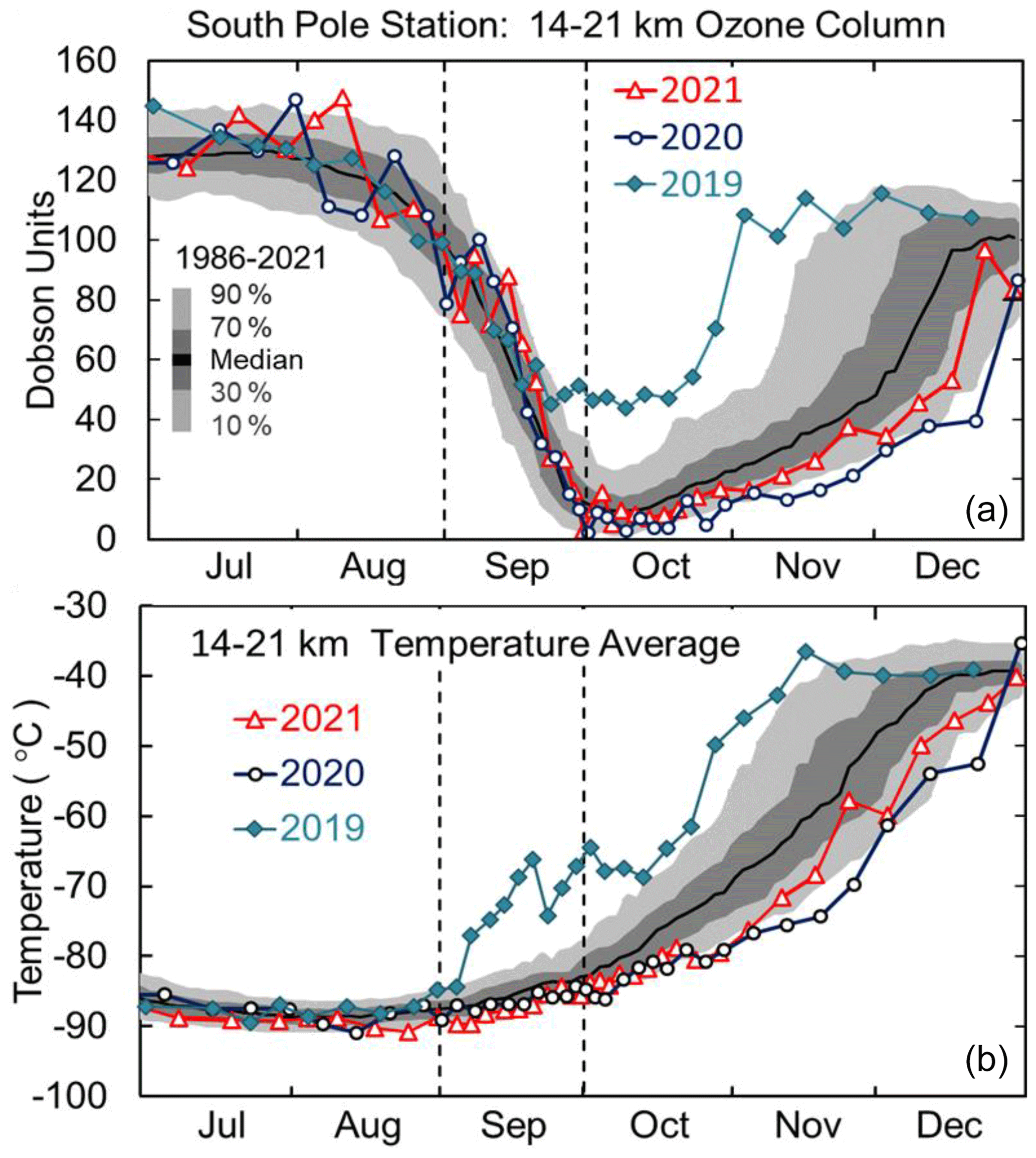
Figure 3Ozonesonde July–December time series in 2019–2021 showing the 14–21 km column ozone in Dobson units (DU) (a) and average temperature (b) compared to the 36-year median (black line) with gray percentile envelopes. The dramatic polar vortex disruption in September 2019 versus cold and stable conditions in 2020 and 2021 shows the extreme variability in September to November measurements that eventually all converge to normal ozone values and temperatures by the end of December.
The stratospheric warming event in 2019 included a large-scale shift in the polar vortex towards the tip of South America (Safieddine et al., 2020) away from the typical position centered near the South Pole. Figure 3 shows the anomalous high-ozone and temperature breakout in early to mid-September 2019 over the South Pole. The 8 September temperature profile showed the first sign of this weakening vortex with an abrupt increase of more than 10 ∘C in the 14–21 km layer. However, the column ozone within the 14–21 km layer remained close to the median line until 20 September when the strong depletion period ended and ozone values leveled off in the 45–50 DU range. Then on 10 October, it dropped to the minimum for the year at 44 DU when the polar vortex briefly centered back over the Antarctic continent and South Pole Station.
The opposite polar vortex conditions were observed in 2020 and 2021 when cold temperatures and column ozone tracked well below the median near the lower edge of the 10–90th percentile line from September through December in Fig. 3. Both years showed severe loss in the 14–21 km column with minimums of 2 DU (1 October 2020) and 3 DU (1 October 2021). The daily Dobson TCO observations also tracked the slow return to typical seasonal values. The latest date the South Pole exceeded the 220 DU ozone hole threshold value (Stolarski et al., 1990) was 12 December 2020 when 236 DU was measured nearly 2 months after the South Pole Dobson observed 109 DU in mid-October. The NASA satellite observations also showed the longest-lived ozone hole on record in 2020 due to the very weak planetary-scale wave activity (Kramarova et al., 2021).
Table 2 lists the altitude layer metrics presented in this study related to ozone loss during September and the minimum ozone occurring by early October. While the lowest ozone is a key metric of ozone hole severity each year, many recovery indices focus on the September observations when the highest sensitivity and correlation with decreasing ODSs may be ascribed (Solomon et al., 2016; de Latt et al., 2017; Pazmiño et al., 2018; Strahan et al., 2019). The South Pole ozonesonde metrics here focus on the 14–21 km layer and include two additional metrics showing an update of the mixing ratio loss rate profiles at selected pressure levels from Hassler et al. (2011a) and a metric showing the yearly vertical extent of layers with near-zero ozone.
Table 2Altitude layers and metrics updated for the 1986–2021 ozonesonde record at the South Pole.
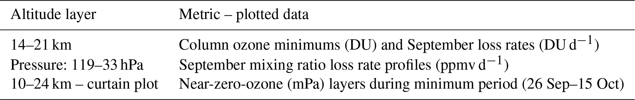
Dobson units (DU), mixing ratio (parts per million by volume – ppmv), millipascals (mPa), and hectopascals (hPa).
Figure 4a shows an overview of the 36-year time series of selected 14–21 km integrated column ozone values representing three stages of the ozone hole over the South Pole. This panel shows the winter average ozone observed before depletion begins and the spring minimum-ozone series. An additional series shows the 15 September values when an ozonesonde is launched each year on this date to track the progress of ozone depletion (Hofmann et al., 2009).
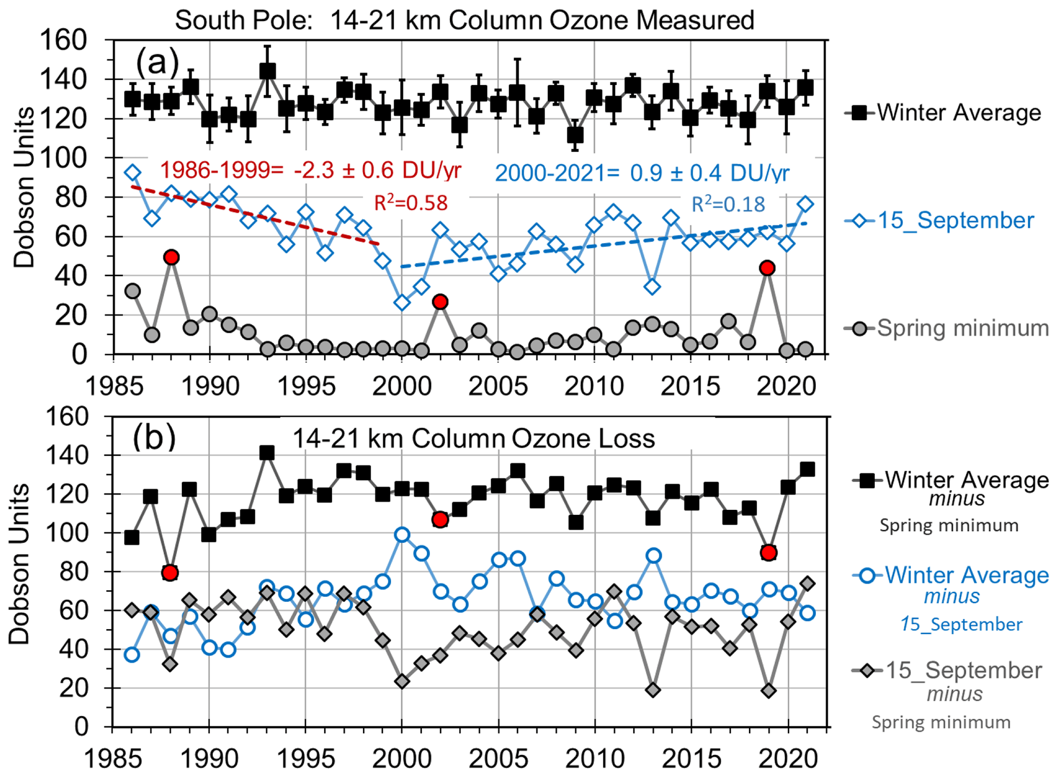
Figure 4(a) The 1986–2021 yearly observations of 14–21 km column ozone over the South Pole showing the winter (15 June–15 August average), 15 September, and the spring minimum ozone in Dobson units (DU). The two dashed lines show the simple regression linear trends and R2 values for all 15 September measurements before and after 2000. (b) The lower panel shows the difference between the three time series in the upper panel to illustrate maximum column ozone loss, the loss during the first half of September (blue open-circle line), and second half (gray diamond line) of the depletion period after 15 September.
The winter average 14–21 km column ozone (15 June–15 August) has been relatively constant at 130 ± 10 DU. The spring minimum-ozone series bottomed out at near-zero ozone from 1993–2001 followed by an upward trend after 2001. The long-term trends in 14–21 km column ozone are more evident in the 15 September series when the 1986–1999 period showed ozone decreasing at a rate of −2.3 ± 0.6 DU yr−1. This was followed by an upward trend line at +0.9 ± 0.4 DU yr−1. The simple linear regression lines in Fig. 4a were computed by the “least squares” method. The uncertainty is the standard error in the slope.
Both the spring minimum and the 15 September series show year-to-year variability. However, the three anomalous polar vortex breakup years (red dots) stand out as peaks in the minimum series, while the 15 September observations showed almost no signal. This may be attributed to the South Pole being near the center of the ozone hole during early September, far from the vortex edge where there is greater dynamical influence on ozone observed (Hassler et al., 2011b). Also, the first signs of the polar vortex weakening typically appear as layers of higher ozone and sudden increases in temperature above 24 km altitude at South Pole Station.
The lower panel (Fig. 4b) shows the result of subtracting selected series in Fig. 4a in order to illustrate the 14–21 km layer total ozone loss each year (winter average minus the spring minimum) and the loss that occurred before and after 15 September. From 1991–2000, there was an increasing trend in the 14–21 km column ozone loss during the first half of September (blue line in Fig. 4b) reaching a peak of 100 DU loss in 2000. This was followed by a downward trend with significant variability, until reaching a relatively stable 60–65 DU after 2014. The loss during the second half of September depends on the amount of ozone remaining on 15 September and meteorological conditions governing the stability of the polar vortex. An early vortex weakening or breakup may result in transport and mixing of high-ozone air masses with the depleted ozone thus reducing or ending loss before the end of September. The year 2021 shows the second-highest overall loss on record at 133 DU. This year began at a slower than average pace with only 59 DU of ozone loss by 15 September but followed with a record loss of 74 DU for the second half of September when only 3 DU remained in the 14–21 km layer on 1 October.
4.1 September column ozone loss rates: 14–21 km
The South Pole September 14–21 km column ozone loss rate is a key metric suggested by Hofmann et al. (1997, 2009) for observing changes related to potential recovery in stratospheric ozone. The metric is useful since the rapid ozone loss during the month of September follows a nearly linear decline which can be compared with the 1986–2021 median loss rate of DU d−1 (see Fig. 3).
Figure 5 shows the yearly September ozone column (14–21 km) loss rates from the ozonesondes launched every 2–4 d during late August until mid-October. The selection of the start and end day for the ∼30 d loss period is adjusted forward or backward by ±3 d to obtain the best linear fit to the observations (see method description in Hassler et al., 2011a). In late September, near the minimum date, the linear depletion data point selection ends when a sharp increase in ozone either is observed or, in severe depletion years, drops to near-zero or shifts to a nonlinear loss rate when approaching ozone loss saturation. The selected values between the start and end points are used to determine the yearly loss rate slope and uncertainty by simple linear regression. The 36-year time series shows that the 14–21 km column ozone loss rate has increased (lower ozone loss rate) from a minimum of −3.8 DU d−1 during 2002–2007 to −3.0 DU d−1 in 2016–2021. The sudden stratospheric warming in 2002 (red dot) showed rapid ozone loss but within a shortened time period ending on 22 September. This was the date when the first sign of the sudden stratospheric warming (increase in ozone and temperature) began to show at altitudes above 21 km. The following ozonesonde profile on 25 September 2002 showed substantial ozone increases throughout the 15 to 32 km layer elevating TCO to 397 DU, the highest ever observed during September and October over the South Pole. In 2019, the loss rate calculation period was also shortened to just 2 weeks before the linear ozone decline ended on 15 September. The loss rate data point for 2019 is included in Fig. 5 with high uncertainty.
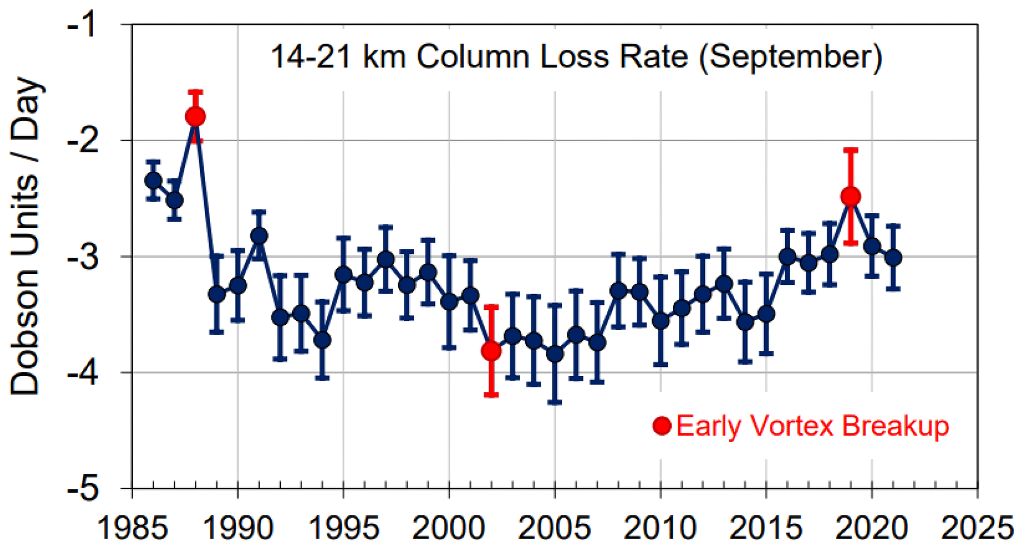
Figure 5Linear loss rates (DU d−1) within the 14–21 km column during 1–30 September. The yearly data include 1σ uncertainty bars. The loss rates calculated for the three anomalous vortex years, shown as red dots, do not include any measurements after the vortex disruption was observed in middle to late September.
4.2 September ozone mixing ratio loss rates: 119–33 hPa
Hassler et al. (2011a) analyzed vertical profiles of ozone mixing ratio loss rates during September in 20 layers from 200 to 10 hPa showing that peak loss rates occurred within the 48 and 33 hPa layers. The 89 hPa pressure level was found to be the optimum layer for detecting significantly lower loss rates based on model estimates of future declining equivalent effective stratospheric chlorine (EESC) and lower variability in measured ozone loss at this level. Early detection was estimated to occur sometime within the 2017–2021 period.
Figure 6 shows the September ozone mixing ratio loss rates (ppmv d−1) for five selected pressure levels from 119 hPa (13.6 km) to 33 hPa (20.6 km). Following the analysis method by Hassler et al. (2011a), the ozone mixing ratios during September (∼ days 235–270) are grouped in 5-year intervals to reduce the influence of prevailing phases of the quasi-biennial oscillation (QBO) and other dynamical processes affecting temperature, meridional transport, and mixing depending on polar vortex conditions. Figure 6 shows that overall loss rates peaked during 2001–2005. All the selected pressure levels showed decreases in loss rates by 2016–2020. The 89 hPa loss rate showed improvement (29 % decrease) with the lowest variability as predicted in the Hassler et al. (2011a) assessment. The highest altitude layer at 33 hPa showed a substantial 49 % decline from the 2001–2005 peak loss rate.
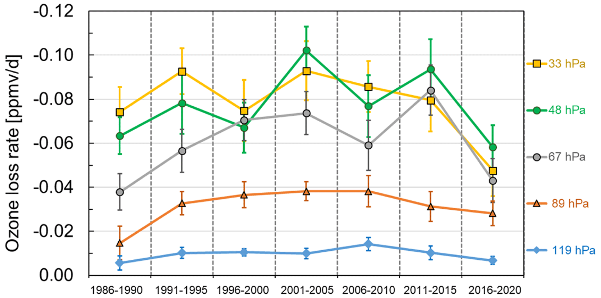
Figure 6September loss rates (ppmv d−1) calculated within 5-year blocks at five selected pressure levels within the primary depletion layer from 119 hPa (13.6 km) to 33 hPa (20.6 km) at the South Pole. The linear fit to the data includes 1σ uncertainty bars.
Figure 7 shows the 1986–2021 temperature time series for the five pressure levels during the month of September and during winter before sunrise from 15 July to 15 August when stratospheric temperatures remain cold (−90 to −94 ∘C) and stable. These data indicate that there have been no systematic winter temperature trends at these altitudes that may affect stratospheric-cloud particle surface area and heterogeneous ozone destruction chemistry. However, 2021 was the coldest September observed at all pressure levels. In addition, Fig. 7 shows that the stable vortex in 2021 remained very cold with almost no temperature difference between winter and September at pressure levels of 119, 89, and 67 hPa and just 2 to 3 ∘C warmer at 48 and 33 hPa. This was similar to the record-low-ozone year in 2006, but the 2006 temperatures were not as cold as 2021. The highest temperatures occurred in 2002 after the sudden stratospheric warming on 22 September when the 30–50 ∘C increase in temperature observed from 100–20 hPa sent the September temperature average off the scale in Fig. 7.
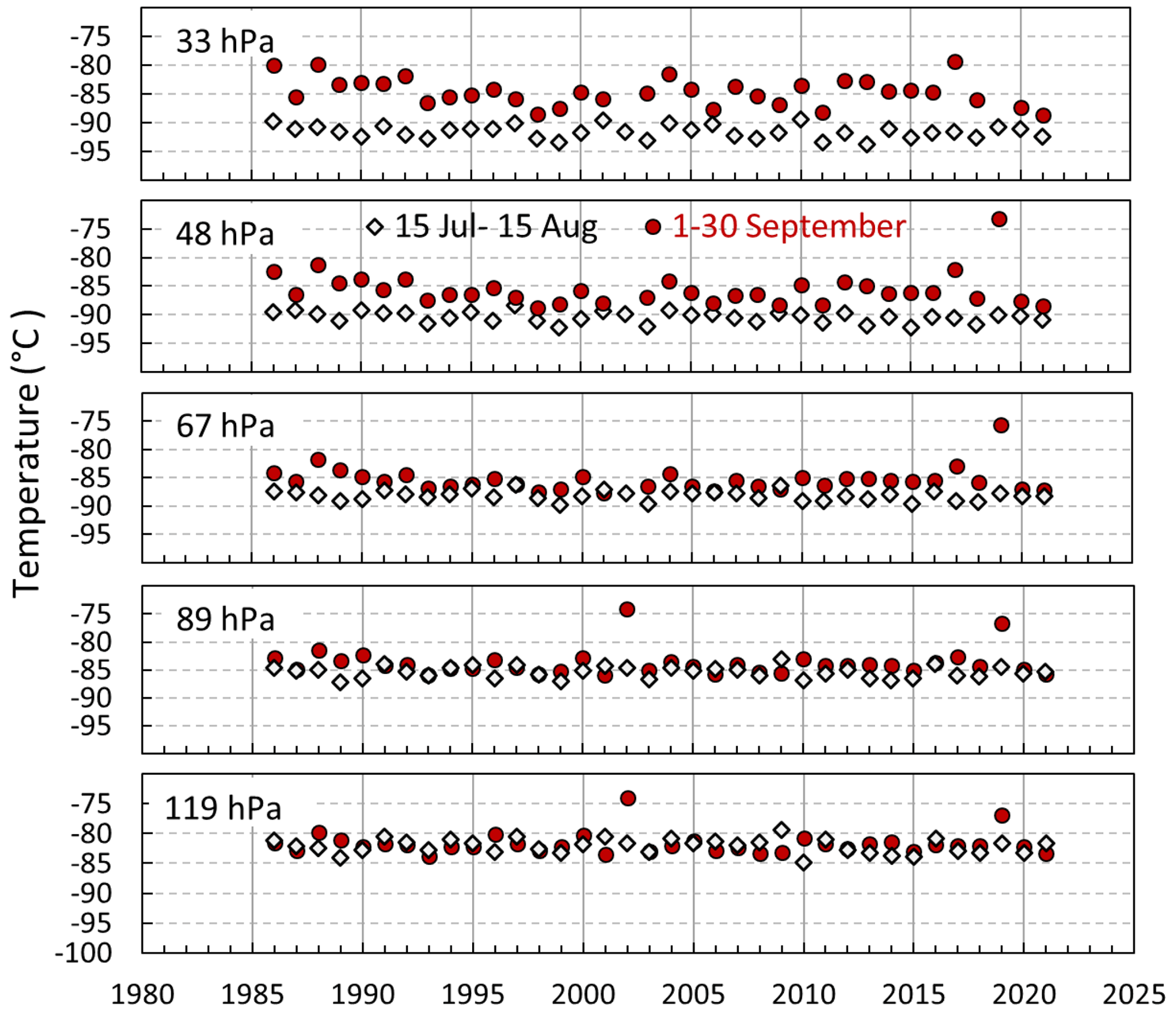
Figure 7Average 30 d winter temperatures from 15 July to 15 August (black diamonds) and during 1–30 September (red circles) from 1986 to 2021. The pressure levels are selected to correspond with the ozone loss rates shown in Fig. 6 within the primary ozone depletion altitude region from 119 hPa (13.6 km) to 33 hPa (20.6 km).
The near-complete destruction of stratospheric ozone (loss saturation) within the 14–21 km layer is a feature of the Antarctic ozone hole that is observed in detail by high-resolution ozonesondes. Near the end of September, as the linear decrease in ozone begins to slow, other nonlinear depletion reactions complete the pathway to near-zero ozone (Grooß et al., 2011; Kuttippurath et al., 2018; Müller et al., 2018). A reduction in the vertical extent of the near-zero-ozone layers will be an important indicator of recovery showing when decreasing EESC is no longer the excess component in the reactions that destroy ozone (Kuttippurath et al., 2018).
The vertical extent of near-zero-ozone layers observed over the South Pole is shown in Fig. 8 as a curtain plot of dark to light gray shaded bars showing only the lowest partial-pressure minimums from 0 to 0.7 mPa. This range of values in the shaded regions represent a 95 %–99 % loss compared to the 14–16 mPa values observed during the winter before ozone depletion begins (see Fig. 2). The near-zero-ozone values for each year are selected from the lowest-partial-pressure ozone out of all seven to nine vertical profiles measured during the ozone hole minimum period (26 September–15 October). All values greater than 0.7 mPa are not included in order to highlight the lowest-ozone region. The three early vortex breakup years, listed in Table 2, are shown as light red bars when ozone minimums were >4–5 mPa.
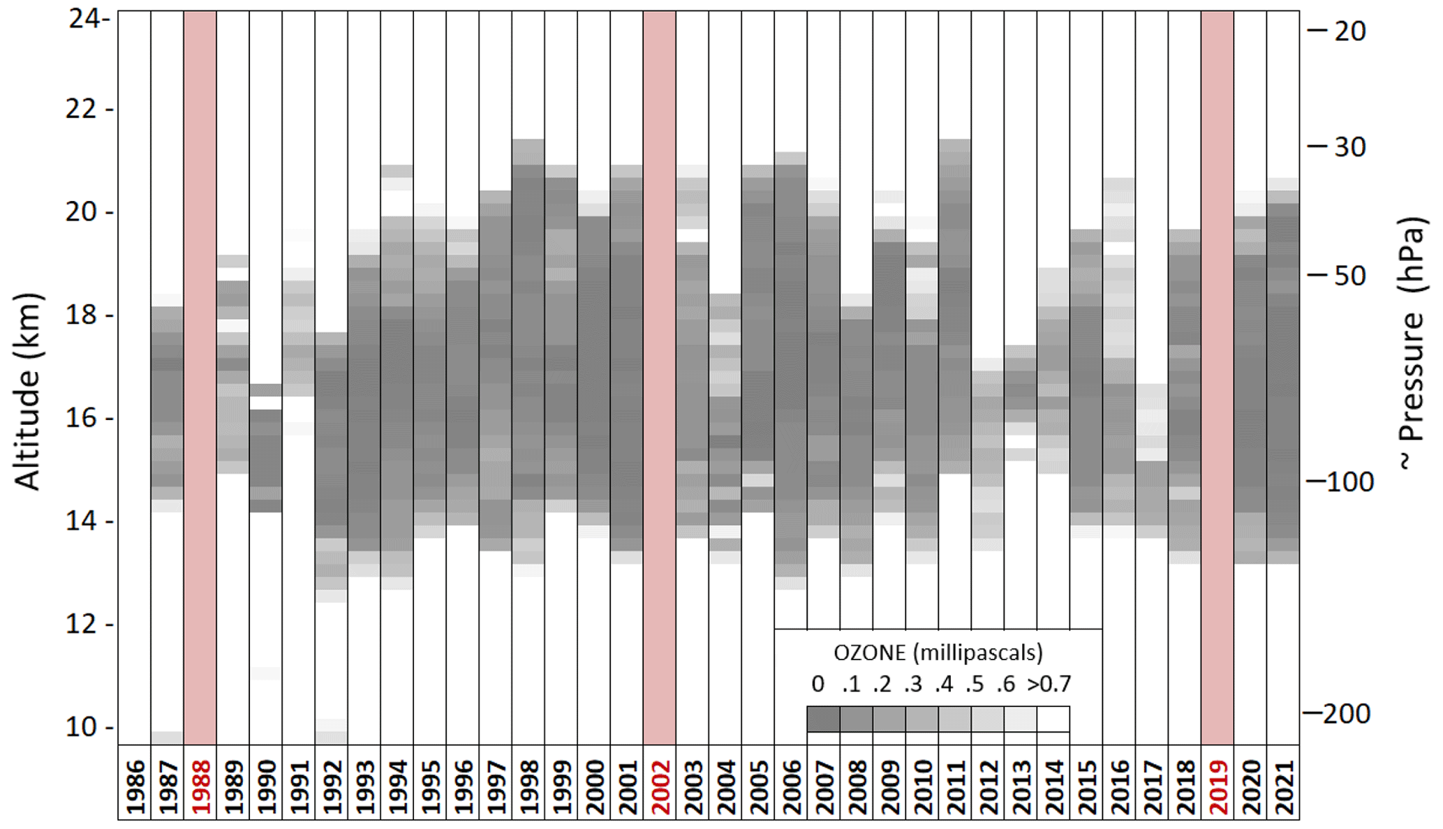
Figure 8The South Pole 10–24 km curtain plots highlighting the lowest observed ozone partial pressure of 0 to 0.7 mPa represented by the dark to light gray shading during the yearly ozone hole minimum period from 24 September to 15 October. All values greater than 0.7 mPa are excluded from the scale shown.
Figure 9 shows the average temperature curtain plot during the minimum-ozone period. The PSC threshold temperature of −78 ∘C is selected as the break point between cold (blue) and warm (red) temperature scales. Together, Figs. 8 and 9 show the coincidence of years with cold temperatures and low ozone. The recurring year-to-year severe depletion from 1991–2001 also shows that the upper boundary of the near-complete ozone loss layer was extending to higher altitudes each year, eventually peaking at 21 km. Hofmann et al. (1997) and Hoppel et al. (2003) noted that a reversal of ozone loss in the upper altitudes may be an important indicator of stratospheric ozone recovery as ODSs decline.
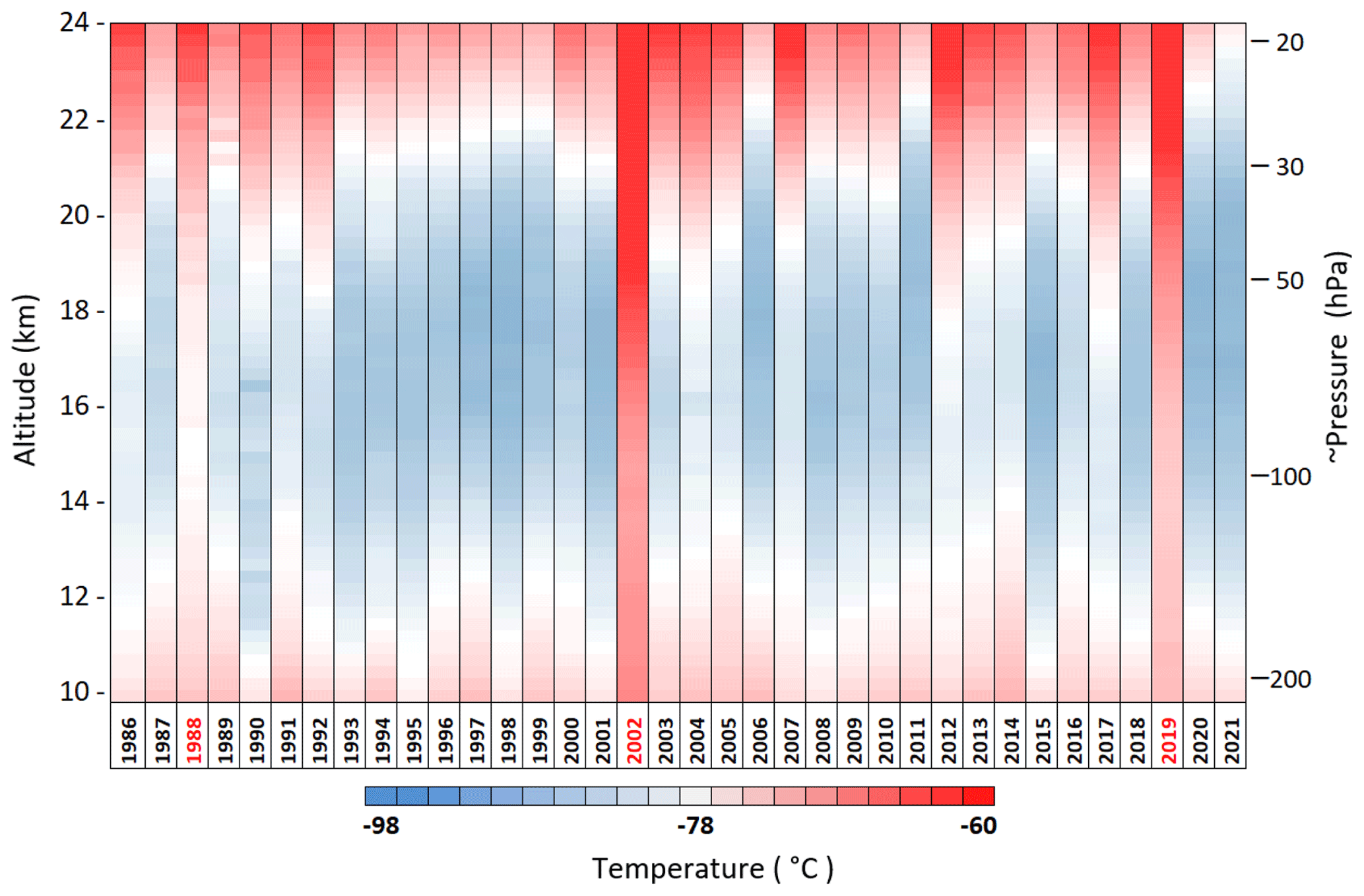
Figure 9The average temperature during 24 September to 15 October (ozone hole minimum period over South Pole Station). The blue to red transition temperature falls at −78 ∘C to highlight the polar stratospheric cloud formation threshold temperature.
Figure 8 shows that after the record low in 2006, the near-zero-ozone vertical extent appeared to be narrowing and becoming irregular. Then in 2020 and 2021 ozonesondes observed the optimum cold polar vortex conditions in September to late October along with extensive near-zero ozone within 13.5 to 20.5 km altitude. However, the 7 km near-zero-ozone layer was not observed in a single profile as it was in the record-low-ozone profile in 2006. For example, in 2021 the near-zero-ozone layer was initially observed at 15–20.5 km on 1 October and from 13.5–17.5 km on 21 October.
Severe ozone loss extending below the 14–21 km layer is not common during the minimum-ozone period over the South Pole. However, the near-zero-ozone region may extend below 14 km following major volcanic eruptions. The transport of volcanic plumes may eventually bring sulfate aerosol into the polar stratosphere leading to additional ozone loss through surface reactions that are similar to PSC heterogeneous chemistry (Hofmann and Solomon, 1989). For example, there was significant depletion from 12–14 km in 1992–1994 after the major eruption of Mount Pinatubo (15.1∘ N; Philippines) in 1991 (Hofmann and Oltmans, 1993; Deshler et al., 1996). The Calbuco eruption (41.2∘ S; Chile) (Bègue et al., 2020) in 2015 also led to an increase in ozone loss below about 14 km (100 hPa) at the South Pole (Stone et al., 2017). More recently, the 15 January 2022 Hunga Tonga–Hunga Ha'apai (20.5∘ S) volcanic eruption plume in the SW Pacific Ocean reached altitudes of nearly 55 km (Carr et al., 2022). This recent mass injection and transport of volcanic aerosols, SO2, and water vapor (Millán et al., 2022; Vömel et al., 2022) may enhance future stratospheric ozone depletion within the Antarctic polar vortex. The ongoing ozonesonde observations along with the 36-year ozone climatology record over the South Pole will assist in identifying any additional ozone loss layers.
Table 3The South Pole yearly ozone hole minimums in total column and 14–21 km partial column ozone and the September loss rates during the long-term record (1986–2021) compared to the record low in 2006 and the extreme variability in the metrics in 2019–2021.

South Pole Station ozonesondes provide essential year-round high-resolution ozone and temperature profiles tracking all phases of the Antarctic yearly ozone hole near the core of the polar vortex, monitoring both the winter development of the vortex and the conditions that lead up to rapid ozone depletion in September, as well as looking precisely in the region where the ozone loss is taking place. The 36-year ozonesonde record has been reviewed, homogenized, and validated by comparing TCO with the South Pole Dobson spectrophotometer DS TCO measurements. Ozonesondes show a positive bias with respect to the Dobson TCO of 2 ± 3 %.
The 2019, 2020, and 2021 South Pole ozonesonde measurements showed the greatest year-to-year variability in ozone hole conditions ever observed in the South Pole long-term record. Table 3 shows several of the key metrics for those years compared to the long-term median and record low in 2006. The anomalous polar vortex warming in 2019 disrupted ozone depletion in early September, resulting in the second-weakest ozone hole on record, but the following 2 years saw cold and persistent vortex conditions with TCO minimums dropping to the 8th and 12th lowest in the 36-year record. In addition, the 2020 and 2021 profiles in early to late October showed near-zero ozone (ozone loss saturation) within the 14–21 km altitude layer under the persistent cold and stable vortex conditions.
The time series (1986–2021) of 14–21 km column ozone during the winter months (15 June–15 August) shows no trend, averaging 130 ± 10 DU. However, rapid ozone loss during 1–30 September at rates of −3.5 ± 0.3 DU d−1 results in 95 %–99 % loss of ozone in the 14–21 km layer. Minimums of near-zero ozone (∼ 1–2 DU) were observed every year from 1993–2001. This was followed by an irregular upward trend from 2002–2021 with the minimum 14–21 km column ozone values ranging from 1–9 DU. The near-zero-ozone minimum years after 2001 include the following: 2003, 2005, 2006, 2011, 2015, 2020, and 2021.
The 15 September 14–21 km column ozone time series indicates a turnaround year in 2000/2001. The simple linear regression lines show decreasing ozone from 1986–1999 at −2.3 ± 0.6 DU yr−1 followed by a reversal to a slight positive trend at +0.9 ± 0.4 DU yr−1 in 2000–2021. This pattern is consistent with several Antarctic ozone hole studies focused on the detection of ozone recovery due to decreasing ODSs (Langematz et al., 2018; Petropavlovskikh et al., 2019).
The September mixing ratio loss rates at selected pressure levels averaged within 5-year blocks all showed improvements by 2016–2020 compared to the peak loss period in 2001–2005. The ozone loss at 33 hPa showed the greatest improvement with a 49 % reduction in loss rate. The optimum pressure level (89 hPa) for detecting significantly lower loss rates showed a 26 % reduction with the lowest variability as predicted by Hassler et al. (2011a).
The long uninterrupted 36-year South Pole ozonesonde record and future balloon-borne measurements provide unique and vital data for ozone hole analyses. The continuing year-round ozonesonde observations at South Pole Station will be beneficial for observing anomalies in the ozone layer driven by meteorological events disrupting the polar vortex and for identifying layers where volcanic aerosols influence ozone depletion.
The South Pole ozonesonde data records are publicly available from the NOAA Global Monitoring Lab (GML) at https://gml.noaa.gov/aftp/ozwv/Ozonesonde/ (NOAA Global Monitoring Lab, 2023). The South Pole ozonesonde data are also made available at https://www.ndacc.org (NDACC, 2022).
BJJ analyzed the data and wrote the manuscript. PC and CS reviewed, edited, and homogenized the long-term ozonesonde data. JB carried out several years of collecting data from ozonesondes and ground-based Dobson. GlM reviewed and provided the ground-based Dobson ozone data. BJJ prepared the manuscript with contributions from all co-authors.
The contact author has declared that none of the authors has any competing interests.
Publisher’s note: Copernicus Publications remains neutral with regard to jurisdictional claims in published maps and institutional affiliations.
This article is part of the special issue “Atmospheric ozone and related species in the early 2020s: latest results and trends (ACP/AMT inter-journal SI)”. It is a result of the 2021 Quadrennial Ozone Symposium (QOS) held online on 3–9 October 2021.
The authors are indebted to the many personnel who conducted the balloon flights over the 36-year period at the South Pole, spending full-year assignments in extreme cold and high-altitude conditions. Without their dedicated service to the US National Oceanic and Atmospheric Administration this work would have been impossible. We thank Allen Jordan, the NOAA/GML/OZWV division programmer/electronics engineer, for the ongoing development of the extremely valuable balloon-tracking telemetry and data analysis SkySonde software. Birgit Hassler was supported by the Helmholtz Society project “Advanced Earth System Model Evaluation for CMIP” (EVal4CMIP). We also acknowledge the logistics support in Antarctica provided by the National Science Foundation, Office of Polar Programs. Finally, we sadly note the passing of coauthor John Booth in June 2021, several months after being diagnosed with an aggressive form of cancer. In 15 years working with NOAA, John spent 11 of those wintering at the South Pole consistently carrying out meticulous ozonesonde and Dobson observations at South Pole Station.
This research has been supported by the US National Oceanic and Atmospheric Administration base funding and observatory operations.
This paper was edited by Jens-Uwe Grooß and reviewed by two anonymous referees.
Allen, D. R., Bevilacqua, R. M., Nedoluha, G. E., Randall, C. E., and Manney, G. L.: Unusual stratospheric transport and mixing during the 2002 Antarctic winter, Geophys. Res. Lett., 30, 1599, https://doi.org/10.1029/2003gl017117, 2003.
Amos, M., Young, P. J., Hosking, J. S., Lamarque, J.-F., Abraham, N. L., Akiyoshi, H., Archibald, A. T., Bekki, S., Deushi, M., Jöckel, P., Kinnison, D., Kirner, O., Kunze, M., Marchand, M., Plummer, D. A., Saint-Martin, D., Sudo, K., Tilmes, S., and Yamashita, Y.: Projecting ozone hole recovery using an ensemble of chemistry–climate models weighted by model performance and independence, Atmos. Chem. Phys., 20, 9961–9977, https://doi.org/10.5194/acp-20-9961-2020, 2020.
Anderson, J. G., Brune, W. H., and Proffitt, M. H.: Ozone destruction by chlorine radicals within the Antarctic vortex – the spatial and temporal evolution of ClO-O3 anticorrelation based on insitu ER-2 data, J. Geophys. Res.-Atmos., 94, 11465–11479, https://doi.org/10.1029/JD094iD09p11465, 1989.
Bègue, N., Shikwambana, L., Bencherif, H., Pallotta, J., Sivakumar, V., Wolfram, E., Mbatha, N., Orte, F., Du Preez, D. J., Ranaivombola, M., Piketh, S., and Formenti, P.: Statistical analysis of the long-range transport of the 2015 Calbuco volcanic plume from ground-based and space-borne observations, Ann. Geophys., 38, 395–420, https://doi.org/10.5194/angeo-38-395-2020, 2020.
Bodeker, G. E., Shiona, H., and Eskes, H.: Indicators of Antarctic ozone depletion, Atmos. Chem. Phys., 5, 2603–2615, https://doi.org/10.5194/acp-5-2603-2005, 2005.
Carr, J. L., Horvath, A., Wu, D. L., and Friberg, M. D.: Stereo plume height and motion retrievals for the record-setting Hunga Tonga-Hunga Ha'apai eruption of 15 January 2022, Geophys. Res. Lett., 49, e2022GL098131, https://doi.org/10.1029/2022gl098131, 2022.
de Laat, A. T. J., van Weele, M., and van der A, R. J.: Onset of stratospheric ozone recovery in the Antarctic ozone hole in assimilated daily total ozone columns, J. Geophys. Res.-Atmos., 122, 11880–11899, https://doi.org/10.1002/2016JD025723, 2017.
Deshler, T., Johnson, B. J., Hofmann, D. J., and Nardi, B.: Correlations between ozone loss and volcanic aerosol at altitudes below 14 km over McMurdo Station, Antarctica, Geophys. Res. Lett., 23, 2931–2934, https://doi.org/10.1029/96gl02819, 1996.
Deshler, T., Stübi, R., Schmidlin, F. J., Mercer, J. L., Smit, H. G. J., Johnson, B. J., Kivi, R., and Nardi, B.: Methods to homogenize electrochemical concentration cell (ECC) ozonesonde measurements across changes in sensing solution concentration or ozonesonde manufacturer, Atmos. Meas. Tech., 10, 2021–2043, https://doi.org/10.5194/amt-10-2021-2017, 2017.
Dhomse, S. S., Kinnison, D., Chipperfield, M. P., Salawitch, R. J., Cionni, I., Hegglin, M. I., Abraham, N. L., Akiyoshi, H., Archibald, A. T., Bednarz, E. M., Bekki, S., Braesicke, P., Butchart, N., Dameris, M., Deushi, M., Frith, S., Hardiman, S. C., Hassler, B., Horowitz, L. W., Hu, R.-M., Jöckel, P., Josse, B., Kirner, O., Kremser, S., Langematz, U., Lewis, J., Marchand, M., Lin, M., Mancini, E., Marécal, V., Michou, M., Morgenstern, O., O'Connor, F. M., Oman, L., Pitari, G., Plummer, D. A., Pyle, J. A., Revell, L. E., Rozanov, E., Schofield, R., Stenke, A., Stone, K., Sudo, K., Tilmes, S., Visioni, D., Yamashita, Y., and Zeng, G.: Estimates of ozone return dates from Chemistry-Climate Model Initiative simulations, Atmos. Chem. Phys., 18, 8409–8438, https://doi.org/10.5194/acp-18-8409-2018, 2018.
Farman, J. C., Gardiner, B. G., and Shanklin, J. D.: Large losses of total ozone in Antarctica reveal seasonal ClOx/NOx interaction, Nature, 315, 207–210, https://doi.org/10.1038/315207a0, 1985.
Grooß, J.-U., Brautzsch, K., Pommrich, R., Solomon, S., and Müller, R.: Stratospheric ozone chemistry in the Antarctic: what determines the lowest ozone values reached and their recovery?, Atmos. Chem. Phys., 11, 12217–12226, https://doi.org/10.5194/acp-11-12217-2011, 2011.
Hassler, B., Daniel, J. S., Johnson, B. J., Solomon, S., and Oltmans, S. J.: An assessment of changing ozone loss rates at South Pole: Twenty-five years of ozonesonde measurements, J. Geophys. Res.-Atmos., 116, D22301, https://doi.org/10.1029/2011jd016353, 2011a.
Hassler, B., Bodeker, G. E., Solomon, S., and Young, P. J.: Changes in the polar vortex: Effects on Antarctic total ozone observations at various stations, Geophys. Res. Lett., 38, L01805, https://doi.org/10.1029/2010gl045542, 2011b.
Hofmann, D. J. and Oltmans, S. J.: Anomalous Antarctic ozone during 1992 - evidence for Pinatubo volcanic aerosol effects, J. Geophys. Res.-Atmos., 98, 18555–18561, https://doi.org/10.1029/93jd02092, 1993.
Hofmann, D. J. and Solomon, S.: Ozone destruction through heterogeneous chemistry following the eruption of El Chichon, J. Geophys. Res.-Atmos., 94, 5029–5041, https://doi.org/10.1029/JD094iD04p05029, 1989.
Hofmann, D. J., Oltmans, S. J., Harris, J. M., Johnson, B. J., and Lathrop, J. A.: Ten years of ozonesonde measurements at the south pole: Implications for recovery of springtime Antarctic ozone, J. Geophys. Res.-Atmos., 102, 8931–8943, https://doi.org/10.1029/96jd03749, 1997.
Hofmann, D. J., Johnson, B. J., and Oltmans, S. J.: Twenty-two years of ozonesonde measurements at the South Pole, Int. J. Remote. Sens., 30, 3995–4008, https://doi.org/10.1080/01431160902821932, 2009.
Hoppel, K., Bevilacqua, R., Allen, D., Nedoluha, G., and Randall, C.: POAM III observations of the anomalous 2002 Antarctic ozone hole, Geophys. Res. Lett., 30, 1394, https://doi.org/10.1029/2003gl016899, 2003.
Johnson, B. J., Oltmans, S. J., Vomel, H., Smit, H. G. J., Deshler, T., and Kroger, C.: Electrochemical concentration cell (ECC) ozonesonde pump efficiency measurements and tests on the sensitivity to ozone of buffered and unbuffered ECC sensor cathode solutions, J. Geophys. Res.-Atmos., 107, 4393, https://doi.org/10.1029/2001jd000557, 2002.
Karpetchko, A., Kyro, E., and Knudsen, B. M.: Arctic and Antarctic polar vortices 1957-2002 as seen from the ERA-40 reanalyses, J. Geophys. Res.-Atmos., 110, D21109, https://doi.org/10.1029/2005jd006113, 2005.
Keeble, J., Braesicke, P., Abraham, N. L., Roscoe, H. K., and Pyle, J. A.: The impact of polar stratospheric ozone loss on Southern Hemisphere stratospheric circulation and climate, Atmos. Chem. Phys., 14, 13705–13717, https://doi.org/10.5194/acp-14-13705-2014, 2014.
Köhler, U., Nevas, S., McConville, G., Evans, R., Smid, M., Stanek, M., Redondas, A., and Schönenborn, F.: Optical characterisation of three reference Dobsons in the ATMOZ Project – verification of G. M. B. Dobson's original specifications, Atmos. Meas. Tech., 11, 1989–1999, https://doi.org/10.5194/amt-11-1989-2018, 2018.
Komhyr, W. D.: Nonreactive gas sampling pump, Rev. Sci. Instrum., 38, 981–983, https://doi.org/10.1063/1.1720949, 1967.
Komhyr, W. D., Reinsel, G. C., Evans, R. D., Quincy, D. M., Grass, R. D., and Leonard, R. K.: Total ozone trends at sixteen NOAA/CMDL and cooperative Dobson spectrophotometer observatories during 1979–1996, Geophys. Res. Lett., 24, 3225–3228, https://doi.org/10.1029/97gl03313, 1997.
Kramarova, N., Newman, P. A., Nash, E. R., Strahan, S. E., Long, C. S., Johnson, B., Pitts, M., Santee, M. L., Petropavlovskikh, I., Coy, L., de Laat, J., Bernhard, G. H., Stierle, S., and Lakkala, K.: 2020 Antarctic ozone hole [in “State of the Climate in 2020”], B. Am. Meteor. Soc., 102, S345–S349, https://doi.org/10.1175/BAMS-D-21-0081.1, 2021.
Kramarova, N. A., Newman P. A., Nash E. R., Strahan, S.E. Strahan, Johnson, B., Pitts, M., Santee, M. L., Petropavlovskikh, I., Coy, L., and De Laat, J.: 2021 Antarctic ozone hole [in “State of the Climate in 2021”], B. Am. Meteor. Soc., 103, S332–S335, https://doi.org/10.1175/BAMS-D-22-0078.1, 2022.
Kuttippurath, J., Kumar, P., Nair, P. J., and Pandey, P. C.: Emergence of ozone recovery evidenced by reduction in the occurrence of Antarctic ozone loss saturation, Npj Clim. Atmos. Sci., 1, 42, https://doi.org/10.1038/s41612-018-0052-6, 2018.
Langematz, U., Tully, M. (Lead Authors), Calvo, N., Dameris, M., de Laat, A. T. J., Klekociuk, A., Müller, R., and Young, P.: Polar stratospheric ozone: Past, present, and future, chapter 4 in scientific assessment of ozone depletion: 2018, global ozone research and monitoring project–Report No. 58. Geneva, Switzerland: World Meteorological Organization, 2018.
Lee, A. M., Roscoe, H. K., Jones, A. E., Haynes, P. H., Shuckburgh, E. F., Morrey, M. W., and Pumphrey, H. C.: The impact of the mixing properties within the Antarctic stratospheric vortex on ozone loss in spring, J. Geophys. Res.-Atmos., 106, 3203–3211, https://doi.org/10.1029/2000jd900398, 2001.
McElroy, M. B., Salawitch, R. J., Wofsy, S. C., and Logan, J. A.: Reductions of Antarctic ozone due to synergistic interactions of chlorine and bromine, Nature, 321, 759–762, https://doi.org/10.1038/321759a0, 1986.
McPeters, R. D. and Komhyr, W. D.: Long-term changes in the total ozone mapping spectrometer relative to world primary standard Dobson spectrometer-83, J. Geophys. Res.-Atmos., 96, 2987–2993, https://doi.org/10.1029/90jd02091, 1991.
McPeters, R. D. and Labow, G. J.: Climatology 2011: An MLS and sonde derived ozone climatology for satellite retrieval algorithms, J. Geophys. Res.-Atmos., 117, D10303, https://doi.org/10.1029/2011jd017006, 2012.
McPeters, R. D., Labow, G. J., and Johnson, B. J.: A satellite-derived ozone climatology for balloonsonde estimation of total column ozone, J. Geophys. Res.-Atmos., 102, 8875–8885, https://doi.org/10.1029/96jd02977, 1997.
Milinevsky, G., Evtushevsky, O., Klekociuk, A., Wang, Y., Grytsai, A., Shulga, V., and Ivaniha, O.: Early indications of anomalous behaviour in the 2019 spring ozone hole over Antarctica, Int. J. Remote Sens., 41, 7530–7540, https://doi.org/10.1080/2150704x.2020.1763497, 2020.
Millán, L., Santee, M. L., Lambert, A., Livesey, N. J., Werner, F., Schwartz, M. J., Pumphrey, H. C., Manney, G. L., Wang, Y., Su, H., Wu, L., Read, W. G., and Froidevaux, L.: The Hunga Tonga-Hunga Ha'apai Hydration of the Stratosphere, Geophys. Res. Lett., 49, e2022GL099381, https://doi.org/10.1029/2022gl099381, 2022.
Montzka, S. A., Dutton, G. S., and Butler, J. H.: The NOAA Ozone Depleting Gas Index: Guiding Recovery of the Ozone Layer, NOAA Earth System Research Laboratory, NOAA, USA, https://gml.noaa.gov/hats/odgi.html (last access: last access: 15 December, 2021), 2021.
Müller, R., Grooß, J.-U., Zafar, A. M., Robrecht, S., and Lehmann, R.: The maintenance of elevated active chlorine levels in the Antarctic lower stratosphere through HCl null cycles, Atmos. Chem. Phys., 18, 2985–2997, https://doi.org/10.5194/acp-18-2985-2018, 2018.
Nash, E. R., Newman, P. A., Rosenfield, J. E., and Schoeberl, M. R.: An objective determination of the polar vortex using Ertel's potential vorticity, J. Geophys. Res.-Atmos., 101, 9471–9478, https://doi.org/10.1029/96jd00066, 1996.
NDACC: Measurement Stations, NDACC [data set], https://www.ndacc.org, last access: 8 August 2022.
Newman, P. A., Kawa, S. R., and Nash, E. R.: On the size of the Antarctic ozone hole, Geophys. Res. Lett., 31, L21104, https://doi.org/10.1029/2004gl020596, 2004.
Newman, P. A., Nash, E. R., Kawa, S. R., Montzka, S. A., and Schauffler, S. M.: When will the Antarctic ozone hole recover?, Geophys. Res. Lett., 33, L12814, https://doi.org/10.1029/2005gl025232, 2006.
NOAA Global Monitoring Lab: Index of /aftp/ozwv/Ozonesonde/, NOAA Global Monitoring Lab [data set], https://gml.noaa.gov/aftp/ozwv/Ozonesonde/, last access: 10 January 2023.
Pazmiño, A., Godin-Beekmann, S., Hauchecorne, A., Claud, C., Khaykin, S., Goutail, F., Wolfram, E., Salvador, J., and Quel, E.: Multiple symptoms of total ozone recovery inside the Antarctic vortex during austral spring, Atmos. Chem. Phys., 18, 7557–7572, https://doi.org/10.5194/acp-18-7557-2018, 2018.
Petropavlovskikh, I., Godin-Beekmann, S., Hubert, D., Damadeo, R., Hassler, B., and Sofieva, V.: SPARC/IO3C/GAW report on Long-term Ozone Trends and Uncertainties in the Stratosphere, SPARC/IO3C/GAW, SPARC Report No. 9, WCRP-17/2018, GAW Report No. 241, https://doi.org/10.17874/f899e57a20b, 2019.
Salby, M. L., Titova, E. A., and Deschamps, L.: Changes of the Antarctic ozone hole: Controlling mechanisms, seasonal predictability, and evolution, J. Geophys. Res.-Atmos., 117, D10111, https://doi.org/10.1029/2011jd016285, 2012.
Safieddine, S., Bouillon, M., Paracho, A. C., Jumelet, J., Tence, F., Pazmino, A., Goutail, F., Wespes, C., Bekki, S., Boynard, A., Hadji-Lazaro, J., Coheur, P. F., Hurtmans, D., and Clerbaux, C.: Antarctic ozone enhancement during the 2019 sudden stratospheric warming event, Geophys. Res. Lett., 47, 14, https://doi.org/10.1029/2020gl087810, 2020.
Schoeberl, M. R. and Hartmann, D. L.: The dynamics of the stratospheric polar vortex and its relation to springtime ozone depletions, Science, 251, 46–52, https://doi.org/10.1126/science.251.4989.46, 1991.
Schoeberl, M. R., Stolarski, R. S., and Krueger, A. J.: The 1988 Antarctic ozone depletion – comparison with previous year depletions, Geophys. Res. Lett., 16, 377–380, https://doi.org/10.1029/GL016i005p00377, 1989.
Smit, H. G. J., Straeter, W., Johnson, B. J., Oltmans, S. J., Davies, J., Tarasick, D. W., Hoegger, B., Stubi, R., Schmidlin, F. J., Northam, T., Thompson, A. M., Witte, J. C., Boyd, I., and Posny, F.: Assessment of the performance of ECC-ozonesondes under quasi-flight conditions in the environmental simulation chamber: Insights from the Juelich Ozone Sonde Intercomparison Experiment (JOSIE), J. Geophys. Res.-Atmos., 112, D19306, https://doi.org/10.1029/2006jd007308, 2007.
Smit, H. G. J. and the Panel for the Assessment of Standard Operating Procedures for Ozonesondes (ASOPOS): Guidelines for homogenization of ozonesonde data, SI2N/O3S-DQA activity as part of “Past changes in the vertical distribution of ozone assessment”, Univ. of Wy, USA, http://www-das.uwyo.edu/~deshler/NDACC_O3Sondes/O3s_DQA/O3S-DQA-Guidelines Homogenization-V2-19November2012.pdf (last access: 15 June, 2021), 2012.
Smit, H. G. J., Thompson, A. M., and the Panel for the Assessment of Standard Operating Procedures for Ozonesondes, v2.0 (ASOPOS 2.0), Ozonesonde Measurement Principles and Best Operational Practices, World Meteorological Organization, GAW Report 268, 2021.
Solomon, S.: Stratospheric ozone depletion: A review of concepts and history, Rev. Geophys., 37, 275–316, https://doi.org/10.1029/1999rg900008, 1999.
Solomon, S., Garcia, R. R., Rowland, F. S., and Wuebbles, D. J.: On the depletion of Antarctic ozone, Nature, 321, 755–758, https://doi.org/10.1038/321755a0, 1986.
Solomon, S., Portmann, R. W., Sasaki, T., Hofmann, D. J., and Thompson, D. W. J.: Four decades of ozonesonde measurements over Antarctica, J. Geophys. Res.-Atmos., 110, D21311, https://doi.org/10.1029/2005jd005917, 2005.
Solomon, S., Ivy, D. J., Kinnison, D., Mills, M. J., Neely, R. R., and Schmidt, A.: Emergence of healing in the Antarctic ozone layer, Science, 353, 269–274, https://doi.org/10.1126/science.aae0061, 2016.
Steinbrecht, W., Claude, H., Schenenborn, F., Leiterer, U., Dier, H., and Lanzinger, E.: Pressure and temperature differences between Vaisala RS80 and RS92 radiosonde systems, J. Atmos. Ocean. Tech., 25, 909–927, https://doi.org/10.1175/2007jtecha999.1, 2008.
Sterling, C. W., Johnson, B. J., Oltmans, S. J., Smit, H. G. J., Jordan, A. F., Cullis, P. D., Hall, E. G., Thompson, A. M., and Witte, J. C.: Homogenizing and estimating the uncertainty in NOAA's long-term vertical ozone profile records measured with the electrochemical concentration cell ozonesonde, Atmos. Meas. Tech., 11, 3661–3687, https://doi.org/10.5194/amt-11-3661-2018, 2018.
Stolarski, R. S., Schoeberl, M. R., Newman, P. A., McPeters, R. D., and Krueger, A. J.: The 1989 Antarctic ozone hole as observed by TOMS, Geophys. Res. Lett., 17, 1267–1270, https://doi.org/10.1029/GL017i009p01267, 1990.
Stone, K. A., Solomon, S., Kinnison, D. E., Pitts, M. C., Poole, L. R., Mills, M. J., Schmidt, A., Neely, R. R., Ivy, D., Schwartz, M. J., Vernier, J. P., Johnson, B. J., Tully, M. B., Klekociuk, A. R., Konig-Langlo, G., and Hagiya, S.: Observing the impact of Calbuco volcanic aerosols on south polar ozone depletion in 2015, J. Geophys. Res.-Atmos., 122, 11862–11879, https://doi.org/10.1002/2017jd026987, 2017.
Stone, K. A., Solomon, S., Kinnison, D. E., and Mills, M. J.: On recent large Antarctic ozone holes and ozone recovery metrics, Geophys. Res. Lett., 48, e2021GL095232, https://doi.org/10.1029/2021gl095232, 2021.
Strahan, S. E., Douglass, A. R., and Steenrod, S. D.: Chemical and dynamical impacts of stratospheric sudden warmings on Arctic ozone variability, J. Geophys. Res.-Atmos., 121, 11836–11851, https://doi.org/10.1002/2016jd025128, 2016.
Strahan, S. E., Douglass, A. R., and Damon, M. R.: Why do Antarctic ozone recovery trends vary?, J. Geophys. Res.-Atmos., 124, 8837–8850, https://doi.org/10.1029/2019jd030996, 2019.
Tarasick, D. W., Davies, J., Smit, H. G. J., and Oltmans, S. J.: A re-evaluated Canadian ozonesonde record: measurements of the vertical distribution of ozone over Canada from 1966 to 2013, Atmos. Meas. Tech., 9, 195–214, https://doi.org/10.5194/amt-9-195-2016, 2016.
Thompson, A. M., Witte, J. C., Sterling, C., Jordan, A., Johnson, B. J., Oltmans, S. J., Fujiwara, M., Vomel, H., Allaart, M., Piters, A., Coetzee, G. J. R., Posny, F., Corrales, E., Andres Diaz, J., Felix, C., Komala, N., Nga, L., Nguyen, H. T. A., Maata, M., Mani, F., Zainal, Z., Ogino, S.-y., Paredes, F., Penha, T. L. B., da Silva, F. R., Sallons-Mitro, S., Selkirk, H. B., Schmidlin, F. J., Stubi, R., and Thiongo, K.: First reprocessing of Southern Hemisphere Additional Ozonesondes (SHADOZ) ozone profiles (1998-2016): 2. comparisons with satellites and ground-based instruments, J. Geophys. Res.-Atmos., 122, 13000–13025, https://doi.org/10.1002/2017jd027406, 2017.
Thompson, A. M., Smit, H. G. J., Witte, J. C., Stauffer, R. M., Johnson, B. J., Morris, G., von der Gathen, P., Van Malderen, R., Davies, J., Piters, A., Allaart, M., Posny, F., Kivi, R., Cullis, P., Nguyen Thi Hoang, A., Corrales, E., Machinini, T., da Silva, F. R., Paiman, G., Thiong'o, K., Zainal, Z., Brothers, G. B., Wolff, K. R., Nakano, T., Stubi, R., Romanens, G., Coetzee, G. J. R., Diaz, J. A., Mitro, S., Mohamad, M., and Ogino, S.-Y.: Ozonesonde quality assurance the JOSIE-SHADOZ (2017) Experience, B. Am. Meteorol. Soc., 100, 155–171, https://doi.org/10.1175/bams-d-17-0311.1, 2019.
Tuck, A. F., Watson, R. T., Condon, E. P., Margitan, J. J., and Toon, O. B.: The planning and execution of ER-2 and DC-8 aircraft flights over Antarctica, August and September 1987, J. Geophys. Res.-Atmos., 94, 11181–11222, https://doi.org/10.1029/JD094iD09p11181, 1989.
Tully, M. B., Krummel, P. B., and Klekociuk, A. R.: Trends in Antarctic ozone hole metrics 2001–17, Journal of Southern Hemisphere Earth Systems Science, 69, 52–56, https://doi.org/10.1071/es19020, 2019.
Van Malderen, R., Allaart, M. A. F., De Backer, H., Smit, H. G. J., and De Muer, D.: On instrumental errors and related correction strategies of ozonesondes: possible effect on calculated ozone trends for the nearby sites Uccle and De Bilt, Atmos. Meas. Tech., 9, 3793–3816, https://doi.org/10.5194/amt-9-3793-2016, 2016.
Vömel, H. and Diaz, K.: Ozone sonde cell current measurements and implications for observations of near-zero ozone concentrations in the tropical upper troposphere, Atmos. Meas. Tech., 3, 495–505, https://doi.org/10.5194/amt-3-495-2010, 2010.
Vömel, H., Evan, S., and Tully, M.: Water vapor injection into the stratosphere by Hunga Tonga-Hunga Ha'apai, Science, 377, 1444–1447, 2022.
Wargan, K., Weir, B., Manney, G. L., Cohn, S. E., and Livesey, N. J.: The Anomalous 2019 Antarctic Ozone Hole in the GEOS Constituent Data Assimilation System With MLS Observations, J. Geophys. Res.-Atmos., 125, e2020JD03333, https://doi.org/10.1029/2020jd033335, 2020.
Witte, J. C., Thompson, A. M., Smit, H. G. J., Fujiwara, M., Posny, F., Coetzee, G. J. R., Northam, E. T., Johnson, B. J., Sterling, C. W., Mohamad, M., Ogino, S.-Y., Jordan, A., and da Silva, F. R.: First reprocessing of Southern Hemisphere ADditional OZonesondes (SHADOZ) profile records (1998–2015): 1. Methodology and evaluation, J. Geophys. Res.-Atmos., 122, 6611–6636, https://doi.org/10.1002/2016jd026403, 2017.
World Meteorological Organization: Scientific Assessment of Ozone Depletion: 2018, Global Ozone Research and Monitoring Project – Report No. 58, Geneva, Switzerland, 572 pp., 2018.
- Abstract
- Introduction
- ECC ozonesonde overview
- South Pole ozonesonde profiles: 2019–2021
- Ozonesonde metrics: altitude intervals: 1986–2021
- Ozone loss saturation: near-zero-ozone layers
- Summary
- Data availability
- Author contributions
- Competing interests
- Disclaimer
- Special issue statement
- Acknowledgements
- Financial support
- Review statement
- References