How aerosol size matters in aerosol optical depth (AOD) assimilation and the optimization using the Ångström exponent

Satellite-based aerosol optical depth (AOD) has gained popularity as a powerful data source for calibrating aerosol models and correcting model errors through data assimilation. However, simulated airborne particle mass concentrations are not directly comparable to satellite-based AODs. For this, an AOD operator needs to be developed that can convert the simulated mass concentrations into model AODs. The AOD operator is most sensitive to the input of the particle size and chemical composition of aerosols. Furthermore, assumptions regarding particle size vary significantly amongst model AOD operators. More importantly, satellite retrieval algorithms rely on different size assumptions. Consequently, the differences between the simulations and observations do not always reflect the actual difference in aerosol amount.

In this study, the sensitivity of the AOD operator to aerosol properties has been explored. We conclude that, to avoid inconsistencies between the AOD operator and retrieved properties, a common understanding of the particle size is required. Accordingly, we designed a hybrid assimilation methodology (hybrid AOD assimilation) that includes two sequentially conducted procedures. First, aerosol size in the model operator has been brought closer to the assumption of the satellite retrieval algorithm via assimilation of Ångström exponents. This ensures that the model AOD operator is more consistent with the AOD retrieval. The second step in the methodology concerns optimization of aerosol mass concentrations through direct assimilation of AOD (standard AOD assimilation). The hybrid assimilation method is tested over the European domain using Moderate Resolution Imaging Spectroradiometer (MODIS) Deep Blue products. The corrections made to the model aerosol size information are validated through a comparison with the ground-based Aerosol Robotic Network (AERONET) optical product. The increments in surface aerosol mass concentration that occur due to either the standard AOD assimilation analysis or the hybrid AOD assimilation analysis are evaluated against independent ground PM_2.5 observations. The standard analysis always results in relatively accurate posterior AOD distributions; however, the corrections are hardly transferred into better aerosol mass concentrations due to the uncertainty in the AOD operator. In contrast, the model AOD and mass concentration states are considerably more accurate when using the hybrid methodology.

1 Introduction

Aerosol transport models describe how particulate pollution is formed from precursor gases, how pollution is transported by atmospheric dynamics, and how it is removed by chemical reactions or deposition. Transport models are an important part of the earth modeling system. Aerosol transport is relevant for understanding and predicting weather and climate because aerosol particles redistribute energy through direct absorption and scattering of (solar) radiation and they serve as nuclei upon which cloud droplets and ice crystals form, thus changing the cloud reflectivity (Twomey, 1977) and cloud lifetime (Albrecht, 1989). Aerosols also play a wider role in atmospheric chemistry and biogeochemical cycles in the Earth system (Andreae and Crutzen, 1997), for example by carrying nutrients to ocean ecosystems (Baker et al., 2003) or nitrogen deposition that significantly affects plant diversity (Bobbink et al., 2010). Air pollution is a major environmental risk to health, and particulates affect more people than any other pollutant. In their 2018 fact sheet, the World Health Organisation estimates air pollution was responsible for 4.2 million premature deaths worldwide in 2016 (World Health Organization, 2018), costing an estimated USD 5.7 trillion or 4.8 % of global GDP (The World Bank, 2019). Air pollution levels continue to rise, the strongest in urban environments in low- and middle-income countries. Aerosol transport models contribute to our understanding of the life cycles of airborne aerosols and hence support effective emission reduction policies, and they are therefore important elements of operational air quality forecast and analysis systems. Despite the enormous importance and efforts to improve models, validation studies (Dennis et al., 2010; Zhang et al., 2012b) continue to report inconsistencies with observations that have different origins, e.g., uncertain emission inventories (Fan et al., 2018), mismatch in transport (Solazzo et al., 2017) and removal procedures (Croft et al., 2012). This also implies that our understanding of how aerosol pollution will respond to mitigation strategies is still quite limited.

The introduction of the 2008 European Directive on Ambient Air Quality and Cleaner Air for Europe encouraged the use of model simulations to perform air quality management tasks such as air quality assessment, forecasting and planning (Europe Environmental Agency, 2011) that were previously performed using measurements. At the same time we see rapid advances in sensor technologies and the availability of aerosol measurements from large-scale network activities that can complement the modeling activities. Those measurements are preferably used to calibrate models and to perform model error corrections through the application of data assimilation techniques (Kalnay, 2002). Examples of popular aerosol measurements used for this purpose are ground-based lidar data (Yumimoto et al., 2008), surface particular matter (PM) concentration observations (Lin et al., 2008; Jin et al., 2018, 2019a), polar-orbiting satellite observations (Schutgens et al., 2012; Khade et al., 2013; Yumimoto et al., 2016a; Di Tomaso et al., 2017; Jin et al., 2022) and geostationary remote sensing data (Yumimoto et al., 2016b; Jin et al., 2019b, 2020). Among available measurements, satellite aerosol products provide valuable information through their high spatial coverage: a single instrument is used to observe a large spatial area making additional harmonization efforts unnecessary.

Using satellite-based observations to improve simulated aerosol concentrations is not straightforward. Aerosol model and remote sensing data are not comparable directly, since the model simulates aerosol mass concentrations, while the sensor measures aerosol optical properties. In order to assimilate aerosol optical data, typically the 3D mass concentration fields are converted into 2D fields of the optical properties retrieved from the measurements. This conversion is performed by a model operator that matches the retrieval algorithm. To obtain retrieved aerosol properties, assumptions need to be made about the aerosol type, size and optical properties in order to obtain quantities such as aerosol optical depth (AOD). However, these assumptions may be inconsistent with similar assumptions in the AOD operator of the aerosol transport model that intends to assimilate the retrievals. At each assimilation cycle some of the difference between the transport-model-derived AOD and the retrieved AOD may simply be due to these inconsistent assumptions. Assimilating the observed radiance as done by Weaver et al. (2007) avoids this inconsistency issue. Using satellite reflectances (radiances) to improve surface concentrations (Drury et al., 2010) and aerosol emissions (Wang et al., 2012; Xu et al., 2013) is another example of an initiative to avoid the mismatch between assumptions in retrieval algorithms and model operators. However, although assimilation of radiances is promising to avoid inconsistencies, other scientific challenges remain. The most notable challenge might be that the information content of space-borne radiance (intensity) measurements is mostly limited to a few degrees of freedom (Veihelmann et al., 2007; Mishchenko et al., 1999; Tanré et al., 1996; Hasekamp and Landgraf, 2005). Consequently, additional a priori information is needed to simulate top-of-atmosphere radiance intensities, such as the solar spectrum, cloud handling, surface reflectance properties, meteorological information (temperature, pressure, humidity), and sun and satellite geometries, and all of these need to be known accurately.

To simulate AOD in a model, the observation operator relies on the chemical composition and aerosol size information from the transport model. Information on size is needed for other processes too, for example aerosol–gas-phase interaction and deposition (Khan and Perlinger, 2017). In transport models aerosol size distributions are represented by sectional (e.g., Jacobson, 2001; Gong et al., 2003; Rodriguez and Dabdub, 2004) or modal (e.g., Ackermann et al., 1998) approaches; the difference between these approaches has been reviewed by Zhang et al. (2002). In this study, the target application of the aerosol modeling is to improve the forecast of particulate matter concentrations, in which the aerosol size is not of major concern; therefore, a modal approach with a diameter-based parametrization is used. Assumptions on aerosol size are part of the parameterization, but these assumptions differ from those made in satellite retrieval algorithms. Harmonization of these assumptions is difficult, for example, because aerosol retrieval algorithms differ per instrument, each with different assumptions on aerosol sizes and other parameters. It is therefore necessary to use different parameterizations of aerosol sizes in the model for each observation operator that is used to simulate retrievals.

Information on the aerosol sizes could be obtained from measurements too. Satellite-based aerosol products are usually reported in several wavelength bands, and the multi-wavelength interpolated Ångström exponent (Ångström, 1929) actually contains aerosol size information. Up to now, this information has only occasionally been used in aerosol studies (Schuster et al., 2006; Saide et al., 2013; Liu et al., 2019). Most of the AOD assimilation efforts only incorporate AOD observations at a single wavelength into the model (referred to as standard AOD assimilation in the whole paper). A few studies assimilated remote sensing aerosol optical products at several wavelength bands; for example Schutgens et al. (2010) assimilated both the Ångström and AOD simultaneously, and Saide et al. (2013) assimilated multi-wavelength AODs. These two studies both assumed that the size-related mismatch between model and observations is due to the uncertainty in the distribution of aerosol emissions over the fine or coarse modes and/or the distribution of aerosol mass over different particle types such as anthropogenic, mineral dust and sea salt. In addition, both assumed that the radius distribution of aerosol types is constant and known, which is not the case for most aerosol mixtures.

In this study, we first explore the role that aerosol sizes play in the conversion of mass concentration to AOD. A common understanding of the role of the particle size in the AOD operator and the retrieval algorithms is necessary when trying to calibrate the AOD computations by comparison with actual AOD observations. Aerosol extinction sensitivity has therefore been studied using an offline AOD operator code based on Mie scattering theory (De Rooij and Van der Stap, 1984). The sensitivity of the AOD calculations to aerosol sizes have been examined. When assimilating AOD observations it is important that assumptions on size are consistent between simulation and retrieval. Therefore, a hybrid AOD assimilation system has been designed that consists of two sequentially conducted steps. The first step aims at estimating the size distribution parameters by assimilating Ångström exponents. The second step aims at estimating the aerosol mass distribution through the assimilation of AOD, using the size distribution parameters just estimated. The hybrid assimilation has been compared to a reference that only assimilates AOD, which might still provide AOD fields that are in agreement with observations but might lead to incorrect mass concentrations. To the best of our knowledge, this is the first time that Ångström assimilation has been coupled with a standard AOD assimilation to optimize the radius parameterizations of aerosol fields.

This paper is organized as follows: Sect. 2 illustrates the Mie-theory-based AOD operator that converts aerosol mass concentrations into AOD values. By employing an offline AOD operator, aerosol extinction sensitivity experiments are conducted to explore the role of aerosol radius in the calculations. Section 3 describes the measurements that have been used in this study for assimilation or independent validation. Section 4 describes the LOTOS-EUROS chemical transport model (CTM) and the configuration used for this study. The hybrid assimilation methodology combining Ångström and AOD assimilation is introduced in Sect. 5 and applied to observations from the MODIS satellite instrument. The increments in surface aerosol mass concentration induced by the assimilations are evaluated using PM_2.5 surface concentration measurements. Section 6 summarizes the results and discusses the added value of using hybrid AOD assimilation.

2 Computation of AOD from aerosol mass concentrations

The aerosol optical depth (AOD) for a certain wavelength is a measure of the extinction of light by aerosols in the atmosphere. Here we describe how AOD is usually computed in a simulation model and specifically the role of the aerosol size distribution in this.

2.1 Aerosol species

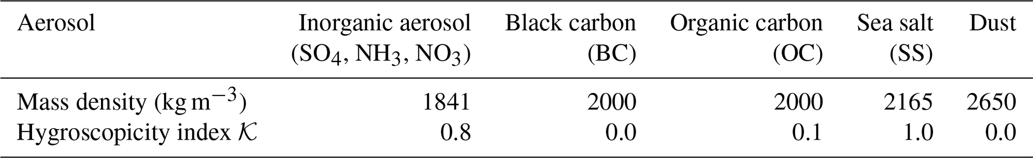
When modeling aerosol concentrations, the aerosol types are often categorized into groups based on their chemical composition. In this study we distinguish five different types: black carbon, organic carbon, mineral dust, sea salt and secondary inorganic aerosol (sulfate, nitrate and ammonium). For the computation of AOD it is necessary to define the specific properties for each aerosol type. The refractive index is a complex number (with a real and an imaginary part) that quantifies the bending and attenuation of light by a layer of aerosols. The hygroscopicity describes the tendency of aerosols to absorb moisture from the surrounding atmosphere, which is important for the AOD since aerosol water has an impact on scattering and absorption by altering aerosol size and refractive index. The hygroscopicity index and mass density for the five types of aerosols used in the following aerosol extinction sensitivity calculations and our aerosol model can be found in Table 1.

Table 1 Mass density and hygroscopicity index for different aerosol types.

2.2 AOD operator

AOD is a direct measure of the total light lost in the atmospheric column, which occurs due to aerosol absorption and scattering along the radiation transmission path. It is, therefore, not directly comparable with simulated 3D aerosol mass concentrations, which is the state calculated in a simulation model. To perform model calibration through AOD observations or to adjust the model using AOD assimilation, an AOD operator (ℋ) is necessary:

$$\begin{array}{}\text{(1)}& {\mathit{\tau }}^{\mathrm{m}}=\mathcal{H}\mathit{X},\end{array}$$

where X denotes the 3D aerosol mass concentration for all aerosol species, and τ^m denotes the 2D field of simulated AOD values. Calibration or assimilation is then based on the difference between the simulation and observations, referred to as the innovation:

$$\begin{array}{}\text{(2)}& \mathit{d}={\mathit{\tau }}^{\mathrm{m}}-\mathit{\tau },\end{array}$$

where τ is the AOD measurement vector.

2.3 Mie theory

In most chemical transport models including the LOTOS-EUROS chemical transport model described in Sect. 4.1, the numerical conversion from aerosol mass concentration into AOD simulation follows the Mie theory. The basis is to calculate the scattering and absorption coefficients of spherical particles with a given radius and refractive index. In the Mie calculation, the model AOD τ^m is defined as a vertical integration of the extinction coefficient ϵ_ext (1 m⁻¹) over n model layers:

$$\begin{array}{}\text{(3)}& {\mathit{\tau }}^{\mathrm{m}}=\sum _{k=\mathrm{1}}^n{\mathit{ϵ}}_{\text{ext}}^k\cdot z^k,\end{array}$$

where ${\mathit{ϵ}}_{\text{ext}}^k$ and z^k denote the extinction coefficient and layer thickness at the kth layer, and ϵ_ext is the product of the dimensionless extinction efficiency 𝒬_ext, the total cross section per unit mass 𝒮 (m² g⁻¹) and the aerosol mass concentration 𝒞 (g m⁻³):

$$\begin{array}{}\text{(4)}& {\mathit{ϵ}}_{\text{ext}}={\mathcal{Q}}_{\text{ext}}\cdot \mathcal{S}\cdot \mathcal{C},\end{array}$$

in which 𝒬_ext equals the sum of scattering efficiency and absorption efficiency. It depends on the ratio of aerosol radius and incident wavelength, as well as the chemical composition (Hulst and van de Hulst, 1981). 𝒮 itself is governed by the particle size and aerosol mass density. Their complex manner will be discussed later in Sect. 2.4.

The Ångström exponent 𝒜 has been introduced for measuring the variability in wavelength-dependent extinction coefficients at different incident wavelengths. 𝒜 is a quantitative indicator of aerosol size (Ångström, 1929); specifically, it reflects the size of aerosols with a sub-micrometer radius (O’Neill et al., 2001). Mathematically, 𝒜 is the slope of the line from the AODs (τ_i, τ_j) at two wavelengths (λ_i, λ_j) when both are on a log-scale:

$$\begin{array}{}\text{(5)}& {\mathcal{A}}_{i-j}=-{\displaystyle \frac{\log ({\mathit{\tau }}_i/{\mathit{\tau }}_j)}{\log ({\mathit{\lambda }}_i/{\mathit{\lambda }}_j)}}.\end{array}$$

2.4 Aerosol extinction sensitivity experiments

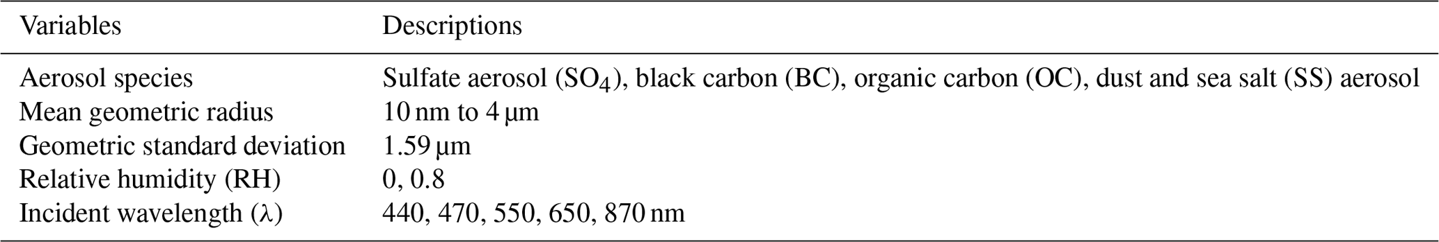
Following Eq. (4), the extinction coefficient is a product of the three individual terms: 𝒬_ext, 𝒮, and 𝒞. To explore the sensitivities of the extinction coefficients to aerosol radius, Mie calculations are performed for aerosols of various sizes and with different refractive indices. The calculation is based on the offline Mie code proposed by De Rooij and Van der Stap (1984). It is slightly different from the Mie code (Boucher, 1998) coupled in our LOTOS-EUROS model, in which the 𝒬_ext calculations from the Mie model are stored in lookup tables for higher computational efficiency. Recently, we showed both of the codes give the exact same result. Aerosol size distributions in LOTOS-EUROS are described using a modal approach. Each mode is represented by a mean geometric radius r_g and a geometric standard deviation σ_g as has been illustrated in Table 4. In the following aerosol extinction sensitivity tests, the independent variable r_g is varied over the range from 10 nm to 4 µm with a step of 10 nm. The control variables associated with the conversion of mass concentration to AOD can be found in Table 2.

The radius-dependent variation in the extinction efficiency 𝒬_ext, total cross section per unit mass 𝒮, extinction coefficients ϵ_ext, and the Ångström exponent 𝒜 of the five aerosol species for two relative humidities (RH = 0 and 0.8) and five wavelengths (λ=440, 470, 550, 650 and 870 nm) are calculated and presented in detail in Figs. S1 to S5, respectively. These five incident wavelengths are employed for the aerosol optical property retrieval in either the Aerosol Robotic Network (AERONET) or MODIS data collection. Parts of the representative results are also shown in Fig. 1 to illustrate the relationship between aerosol extinction and radius.

Table 2 Control variables in the aerosol extinction sensitivity experiments.

2.4.1 Extinction efficiency

The relationship between the extinction efficiency 𝒬_ext and mean geometric radius for sulfate and organic carbon aerosols are presented in Fig. 1a. Small particles are very poorly scattered, and their light absorption capacity is also well below what we may expect from their physical size; the extinction efficiency of particles much smaller than the wavelength of light is therefore ≪1. Very large particles remove twice as much light as we may expect from their geometrical cross section. Physically, this is explained by the sum of light scattered by reflection and refraction within the particle plus the diffracted component that is lost from the direct beam. Particles are most active, or have the highest extinction efficiency, when their sizes are in the range of the wavelength. For single particles that do not absorb light the scattering may be 4 times more efficient than their real size suggests. When considering distributions of particles as in Fig. 1 rather than the combination with less optically efficient particles reduces the maximum in the extinction efficiency. A particle size distribution also removes the well-known maxima, minima and secondary-order ripples in the extinction efficiency curve that are due to the interference of light with spheres that have just the right dimension to diffract and transmit light.

For absorbing aerosol the peak in the scattering efficiency is reduced (e.g., Hansen and Travis, 1974). For non-absorbing aerosol the scattering efficiency curve seems to move to the left for higher real parts of the refractive index; see, for example, Fig. 2 in Moosmüller and Ogren (2017) and our Fig. 1a where the extinction efficiency curve of OC (organic carbon; m_real=1.53, λ=550 nm) peaks at a smaller size distribution than the extinction efficiency curve of SO₄ (m_real=1.43, λ=550 nm). Next to the chemical constituent, the extinction efficiency also depends on the ratio of particle size and wavelength of light, which are usually expressed as a size parameter $x=\mathrm{2}\mathit{\pi }\cdot r_{\mathrm{g}}/\mathit{\lambda }$. As can be seen in Fig. 1a, although the peak of the extinction efficiency is found at a larger size distribution when the incident wavelength is changed from 550 to 870 nm, the peak is actually found at the fixed size parameter x like for the same aerosol species.

Also in Fig. 1a we show the effect of a higher humidity (RH = 0.8). The hydrophilic nature of SO₄ leads to water uptake and thus physical size growth. The smaller dry particles – distributions to the left of the extinction efficiency peak – thus grow into the more optically active region; i.e., the curve and peak move to the left. On the other hand, the uptake of water, with a real part of the refractive index of 1.33, will make the curve move to the right. The net effect of water uptake is a move to the left. Hence the change in size is more important than the change in refractive index.

2.4.2 Total cross section

Figure 1b plots the total cross section per dry mass 𝒮 for sulfate, organic carbon and black carbon aerosols at different size distributions. The total cross section 𝒮 is a product of the mean cross section and total number per dry mass. The former is proportional to the square of the geometric mean radius r_g, while the latter is proportional to the negative cubic power of r_g. In terms of 𝒮, aerosols at a larger size distribution are less effective in diminishing the total solar radiation compared to finer aerosol bins. A steady decline in 𝒮 is therefore found with an increase in the aerosol size distribution over all the species.

For the inorganic aerosols, the hydrophilic characteristic tends to efficiently increase 𝒮. Take SO₄ (hygroscopicity index 𝒦=0.8) for instance: there is a 1.61 times growth in the diameter when they are surrounded by a wet atmosphere (RH = 0.8) following the aerosol diameter hygroscopic growth function $f\left(\text{RH}\right)=\mathit{\{}\mathrm{1}+\mathcal{K}\cdot \text{RH}/(\mathrm{1}-\text{RH}){\mathit{\}}}^{\mathrm{1}/\mathrm{3}}$ (Petters and Kreidenweis, 2007), which is equal to a 2.60 times growth in 𝒮 here. The total cross section 𝒮 of OC is less sensitive to relative humidity since it has a much lower hygroscopicity index (𝒦=0.1). For hydrophobic aerosols like dust and black carbon, their total cross section will not change when they are moved to a wet atmosphere.

We also show the effect of mass density on the 𝒮 calculation. The aerosol with a lower mass density has a larger size, which results in a higher total cross section. The mass density of sulfate, organic carbon and black carbon aerosols are 1841, 2000 and 2000 kg m⁻³. In terms of 𝒮, sulfate aerosol bins are slightly more efficient in diminishing the total solar radiation than the organic carbon and black carbon aerosols when they are at the same size distribution.

2.4.3 Extinction coefficient

The extinction coefficients ϵ_ext are then calculated as a product of 𝒬_ext, 𝒮 and a given dry aerosol concentration 𝒞 (1 g m⁻³) following Eq. (4). The relationship between the aerosol extinction coefficients ϵ_ext and the size distribution r_g are shown in Fig. 1c. In general, ϵ_ext presents an up-and-down pattern: aerosols at a small size distribution result in a low ϵ_ext due to their inactive extinction efficiency 𝒬_ext (see Fig. 1a), while particles at a large size distribution that leads to a small total cross section 𝒮 would result in a low ϵ_ext as well (see Fig. 1b). Particles with a geometric mean radius ranging from tens to hundreds of nanometers are most active in diminishing the solar radiation. The effect of chemical constituent on the extinction coefficient can also be found in Fig. 1c. Black carbon reaches a higher peak at a smaller size distribution than organic carbon and inorganic carbon due to its high extinction efficiency 𝒬 curves at the small size. Water absorption (RH = 0.8) makes the hygroscopic aerosols become more efficient in diminishing the light absorption and scattering; e.g., the ϵ_ext curve and peak of SO₄ aerosol move to the upper left.

The efficient coefficients vary significantly at different sizes distribution. For instance, ϵ_ext of SO₄ at an incident wavelength of λ=550 nm (RH = 80 %) reaches 12.21 (1 m⁻¹) at a geometric mean radius of r_g=110 nm; it reduces rapidly to 4.73 (1 m⁻¹) at r_g=350 nm. Therefore, the 3D conversion from mass concentration to AOD in aerosol models is highly sensitive to the aerosol size distribution. For a fair comparison between the model AODs and actual AOD observations, the aerosol size should remain consistent in the AOD operator and the satellite AOD retrieval algorithm.

2.4.4 Ångström exponent

Following Eq. (5), the Ångström exponent is calculated using the extinction coefficients at two incident wavelengths. The Ångström exponents at 870–440 and 650–470 nm are calculated in this study: the former is used in the AERONET Ångström product, while the latter corresponds to the MODIS Ångström observational wavelengths. The size-dependent Ångström curves for inorganic carbon (SO₄), organic carbon and black carbon aerosols are presented in Fig. 1d. It is worth noting that a continual decline is observed in the Ångström exponent curve for all the species when the aerosol size distribution grows to 400 nm. Subsequently, the Ångström curve remains stable with an increase in the aerosol geometric mean radius. It is evident that the Ångström data contain valuable aerosol size information. Apart from the coarse-mode-dominated dust and sea salt aerosols, inorganic carbon, black carbon and organic carbon aerosols are believed to be fine-mode-dominated and exhibit a mean radius of less than 400 nm. Therefore, Ångström is a key quantitative indicator of aerosol bin sizes.

In real situations, airborne aerosols are a mixture of several species. The extinction coefficients of mixed aerosols equal the sum of ϵ_ext for all species. The Ångström exponent is interpolated using the integrated ϵ_ext at two different incident bands, thus indicating the size distribution of mixed aerosols.

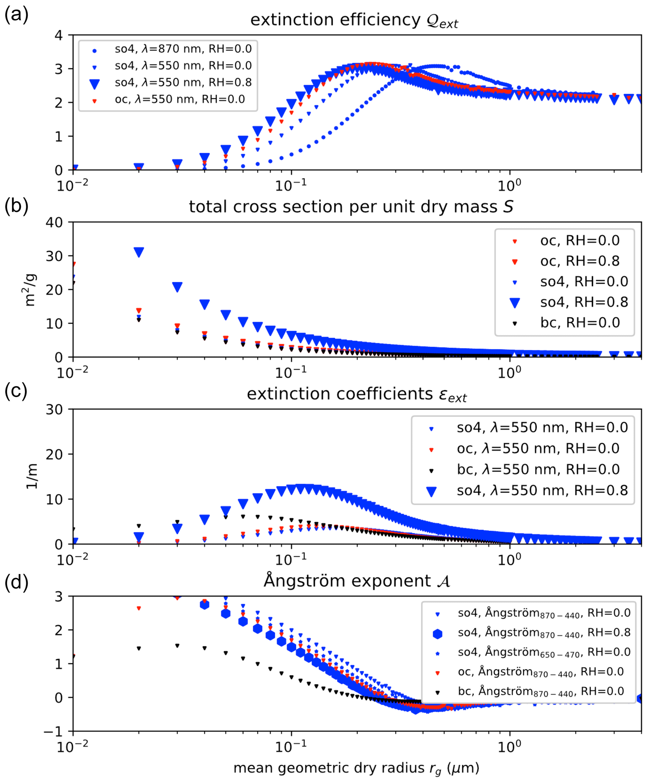
Figure 1 Aerosol extinction vs. mean geometric dry radius r_g. (a) Extinction efficiency 𝒬_ext; (b) total cross section per unit dry mass 𝒮; (c) extinction coefficients ϵ_ext; (d) Ångström exponent 𝒜. Note that λ represents the incident wavelength. Abbreviations: BC: black carbon; SO₄: sulfate aerosols; OC: organic carbon; RH: relative humidity.

3 Measurements

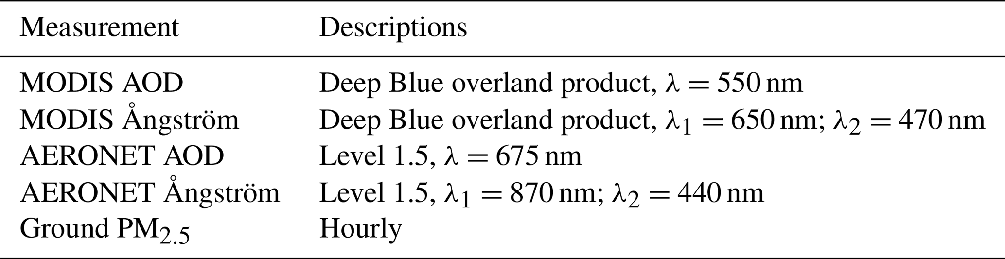
Measurement data from three different sources are used in this study. The Ångström exponent and AOD measurements from MODIS Deep Blue products have been used in the assimilation system that will be described in Sect. 5. The corrections made to the model aerosol size information are validated through a comparison with the AERONET optical products, while the corrections made to the surface aerosol mass concentration simulation are evaluated using independent ground PM_2.5 observations. The datasets and relevant information are summarized in Table 3.

3.1 MODIS

In this study, Deep Blue aerosol products (Hsu et al., 2013; Sayer et al., 2014) of the Moderate Resolution Imaging Spectroradiometer (MODIS) C6.1 data suite have been used in the aerosol assimilation system. Its Ångström exponent 𝒜_650−470 is assimilated to estimate the aerosol radius, while its AOD data τ₅₅₀ are assimilated to estimate the aerosol mass concentration field. The assimilation of MODIS aerosol properties is conducted in the original MODIS observational space. Specifically, each of the MODIS measurements is compared to the aerosol simulation at the grid cell that is holding the MODIS pixel.

Snapshots of MODIS AOD and Ångström captured on 24 July (between 10:00–11:00 UTC) are presented in Fig. 2a and b. Most MODIS AOD observations stay in the range from 0.05 to 0.8. Ångström exponents exhibit less spatial variability, and most values stay around 1.2 to 1.6. However, there are still some low Ångström exponents, for instance, the ones in the green-colored region in Fig. 2b, which have been validated as inconsistent measurements in Sect. 3.2.

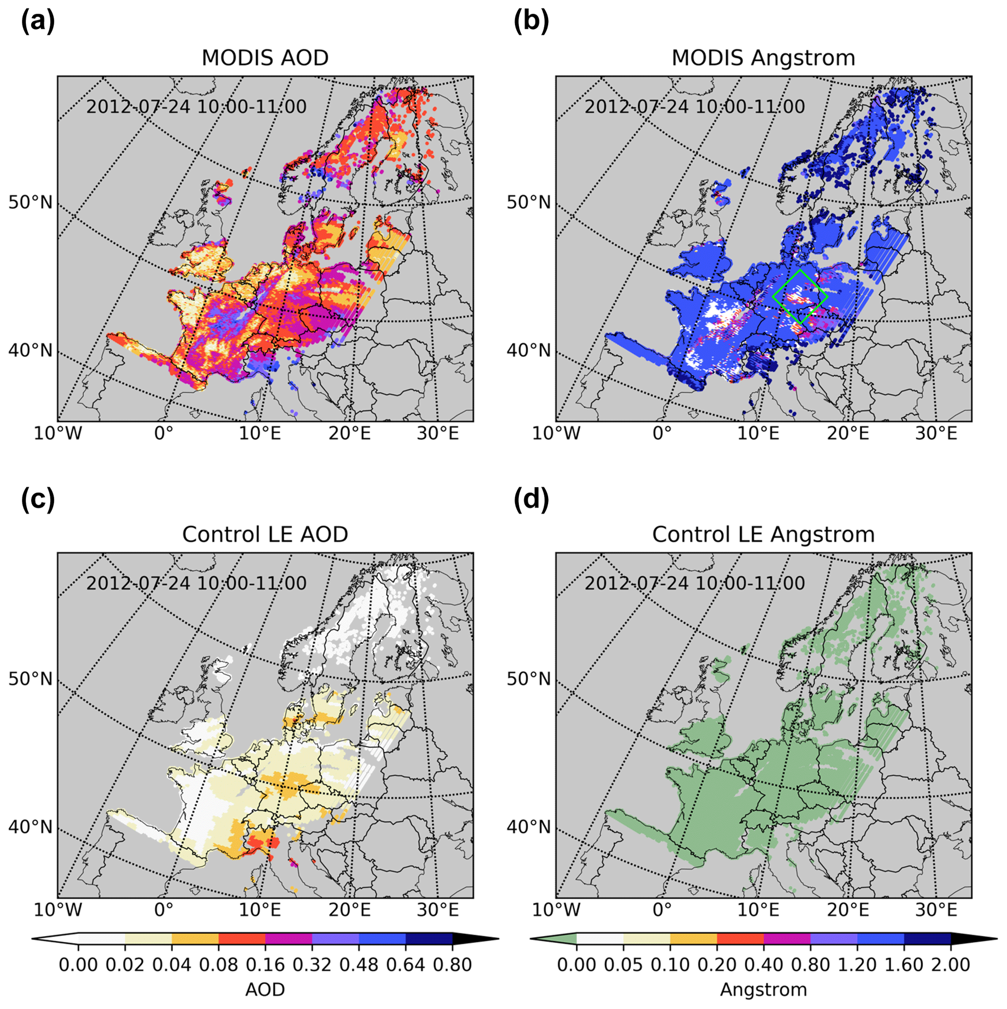
Figure 2 MODIS AOD, MODIS Ångström, control LOTOS-EUROS (LE) AOD₅₅₀ and control Ångström_650−470. Although LE AOD and Ångström can be simulated anywhere, they are only projected into the MODIS space for making the comparison easier. Gray pixels indicate observation vacancy.

3.2 AERONET

The MODIS product is first evaluated through a comparison with ground-based observations collected from the Aerosol Robotic Network (AERONET). At the sites of this network, the total number of AOD columns is measured using ground sun photometers. AOD and Ångström measurements at Cabauw and Leipzig have been used for validation. The locations of these two AERONET sites are marked in Fig. 5. Figures 3 and 4 show the time series of AERONET AOD and Ångström observations at these two sites from the level 1.5 product (cloud-screened and quality controlled). MODIS AODs and Ångströms at 500 nm are also shown as an average over the 0.1^∘ × 0.1^∘ model grid cell in which the site is located.

The time series reveal that the MODIS AOD and Ångström observations match the spread in the AERONET observations well. There are also some inconsistent MODIS Ångström values that did not match the AERONET measurements all the time. Specifically, we have several MODIS Ångström measurements around 0 at the Leipzig site, as shown in the green-colored region in Fig. 4b; meanwhile, the nearby MODIS Ångström exponents and AERONET measurements exhibit high levels. The 0 MODIS Ångström exponent at Leipzig on 24 July refers to the pixels in the green-colored region (Fig. 2b). These local inconsistent Ångström observations are supposed to occur due to the retrieval error, which might prevent us from exploring fine-scale aerosol size distributions in Sect. 5.1.2.

AERONET AOD and Ångström observations are calculated at wavelengths (pairs) different from those used to interpolate the MODIS Deep Blue aerosol product; the details are presented in Table 3. They are the only aerosol optical products released for the two AERONET stations (Cabauw and Leipzig) and the MODIS Deep Blue product for vegetated lands. To accurately calculate the AOD and Ångström difference between simulations and observations, our LOTOS-EUROS model simulated the AODs and Ångström exponents at all these wavelengths (pairs).

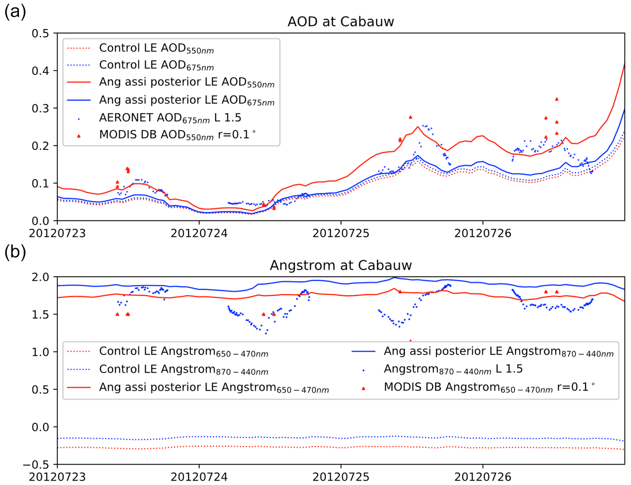
Figure 3 AERONET, MODIS and LOTOS-EUROS prior AOD (a) and Ångström (b) at Cabauw (51^∘58' N, 04^∘55' E). Note that r defines the radius for mapping the MODIS product into test sites. Observations from AERONET and the consistent LE simulations are marked in blue; observations from MODIS and the comparable simulations are shown in red.

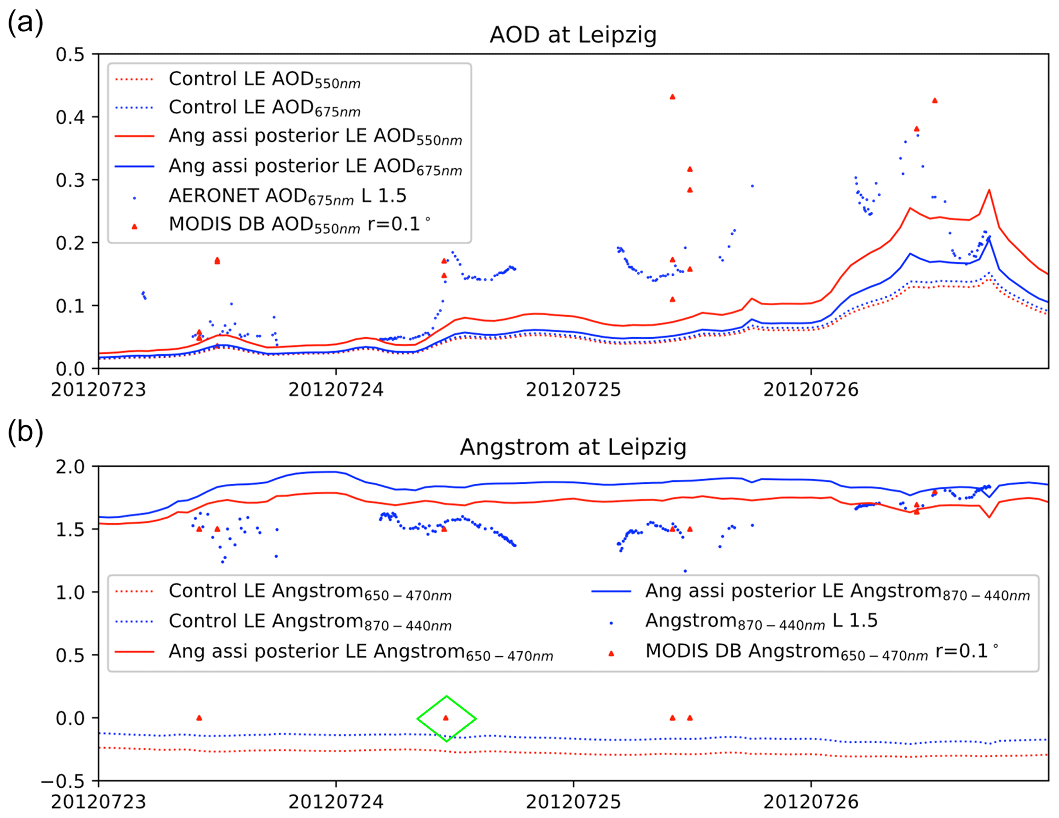
Figure 4 AERONET, MODIS and LOTOS-EUROS prior AOD (a) and Ångström (b) at Leipzig (51^∘21' N, 12^∘26' E). Note that r defines the radius for mapping the MODIS product into the test site.

3.3 Ground PM_2.5 concentration

The focus of aerosol models and remote sensing data assimilation is to achieve accurate estimation of the aerosol state field, which would subsequently move forward an accurate forecasting of aerosol mass concentrations. In this study, hourly PM_2.5 observations over 151 EU air quality ground stations have been collected to validate the model simulations on surface aerosol concentrations. The distributions of these ground stations are shown in Fig. 5. Although other air quality monitoring stations were available during our study, they only provide daily-averaged aerosol measurements. They have large uncertainties for representing the instant aerosol loading measured by the MODIS instruments, and therefore they are not used here.

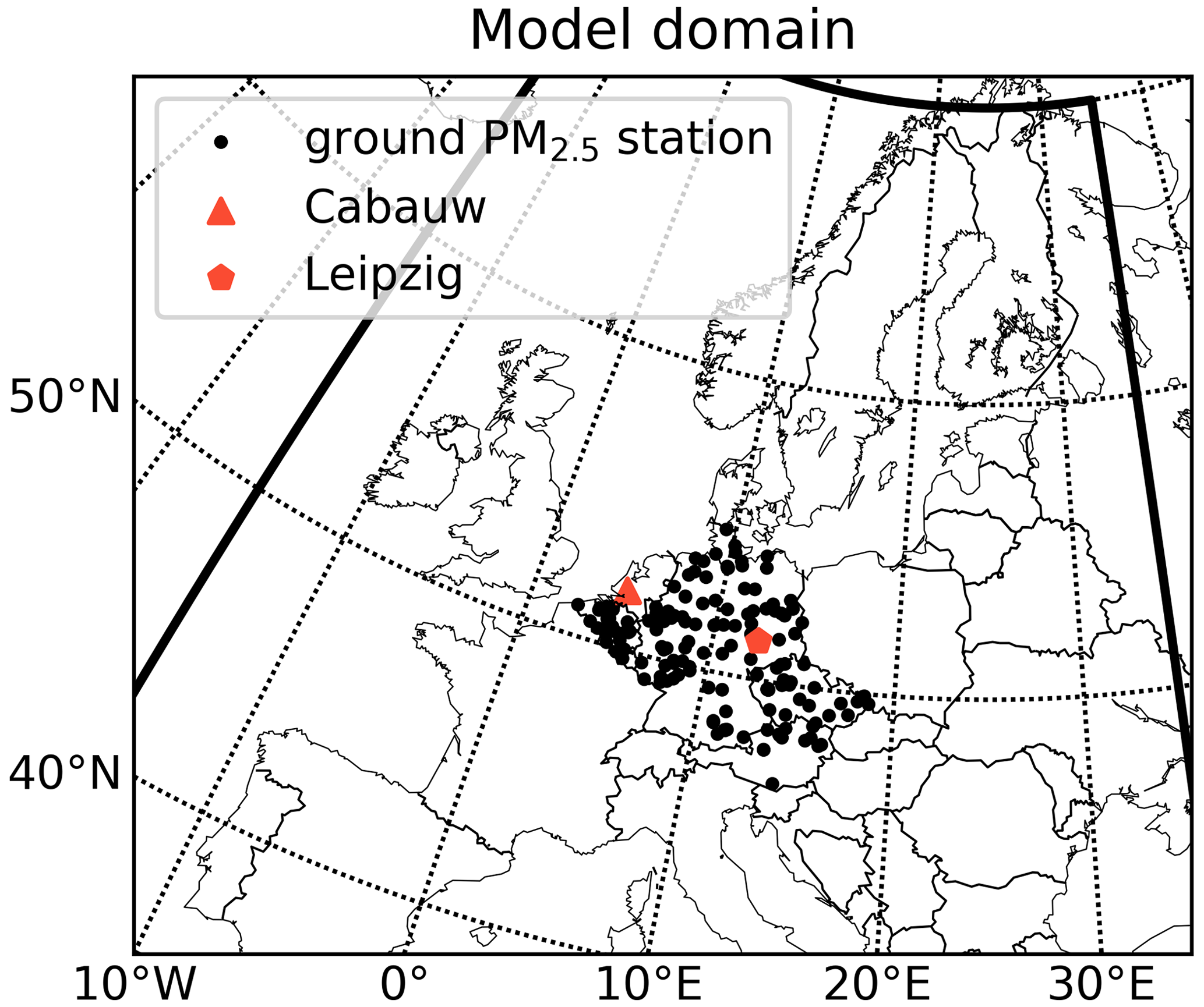
Figure 5 Model domain and locations of ground PM_2.5 stations and AERONET sites at Cabuaw and Leipzig.

Table 3 Measurements for assimilation and validation.

4 Model description

The satellite observations of AODs and derived Ångström exponents will be assimilated with model simulations to obtain the best possible representation of aerosol concentrations. For the simulations a regional chemical transport model (CTM) will be used, which is described in Sect. 4.1. As reference for the assimilation experiments, a standard simulation has been performed, which is described in Sect. 4.2.

4.1 Model description and aerosol size distribution

The regional chemistry transport model (CTM) LOTOS-EUROS will be used to simulate aerosol concentrations. This simulation model has been used for a wide range of applications related to air quality simulations, forecasts and scenario studies both inside and outside of Europe (Manders et al., 2017).

For the current study, the LOTOS-EUROS model has been configured over a domain from 35 to 70^∘ N and 15^∘ W to 35^∘ E (shown in Fig. 5), with a resolution of 0.25^∘ × 0.25^∘ (about 15×25 km at these latitudes). In the vertical a simple mixing layer approach is used with only five layers in total: a surface layer of 25 m, a mixing layer, two reservoir layers and a top layer that reaches an altitude of 5 km. This rather coarse configuration allows fast simulation of the main trace gas and aerosol concentrations. Physical processes included are emission, advection, diffusion, dry and wet deposition, and sedimentation. Anthropogenic emissions of trace gases and aerosols are taken from a TNO emission inventory (Kuenen et al., 2014). The partitioning of nitrate and ammonium between the gas and aerosol phase is described using ISORROPIA (Fountoukis and Nenes, 2007). Natural emissions of dust and sea salt aerosols are calculated online given surface characteristics and meteorology.

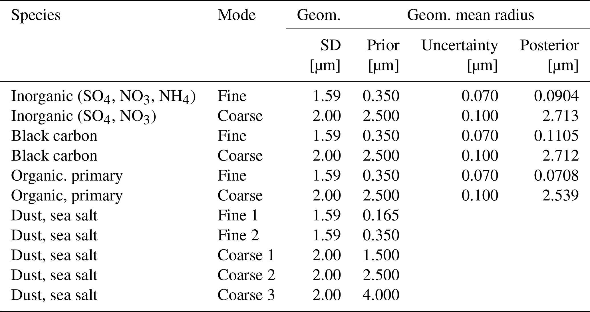
The gas-phase chemistry is based on a carbon-bond mechanism. Aerosol concentrations are represented by 21 different species corresponding to particles with a specific chemical composition within a certain size mode. A size mode characterizes a distribution of aerosol radii following a lognormal distribution, defined by its geometric mean and standard deviation. For most aerosol types two size modes are defined to characterize a fine and a coarse model; for dust and sea salt aerosols, two fine and three coarse modes are used that allow more detailed modeling of emission and deposition processes. The prior geometric mean and standard deviation of the aerosol species are provided in Table 4. The table also includes numbers for uncertainty and posterior estimates of the geometric mean, which are input and output of the assimilation procedure.

A considerable amount of the literature on ground observations indicated that there is remarkable spatial and temporal variation in the aerosol size distribution, e.g., the geometric mean radius ranging from tens to hundreds of nanometers (Costabile et al., 2009). It is insufficient to describe these spatiotemporally varying characteristics using a fixed value that is used in practice. Using a fixed value, the model AOD and Ångström exponents are likely to be strongly biased, as will be discussed in Sect. 4.2, and the AOD assimilation result will be misleading, as is illustrated in Sect. 5.3. Meanwhile, comparisons against other aerosol models, e.g., WRF-Chem (Palacios-Peña et al., 2020) and ECHAM-HAM (Zhang et al., 2012a), indicated our aerosol size assumptions differ from them to some extent (mainly overestimated). Therefore, as a first step to improve the AOD simulations, we assign the mismatch between the simulated and observed Ångström exponents only to the errors in the assumption of aerosol radii in our Ångström assimilation.

The standard deviations (SDs) are another key factor of the aerosol size distribution. The same choice as used in this study is present in several other aerosol models. For instance, ECHAM-HAM (Zhang et al., 2012a) and EC-Earth3 (van Noije et al., 2021) also use 1.59 and 2.0 for characterizing the SDs of fine and coarse aerosol distributions, respectively. Similar choices (1.6 and 2.0) were also used in GEOS-Chem for describing their sulfate aerosols (Yu and Luo, 2009). The SD of the size distribution is therefore assumed to be more certain in this study.

Our hybrid AOD assimilation method that will be described in Sect. 5 has been tested over Europe for the period 23 to 26 July 2012. This period was chosen because hardly any clouded pixels were present in these 4 d, and therefore many high-quality satellite observations are available.

Table 4 Geometric means and standard deviations used for aerosol radius size distributions in this study. The columns for (prior) uncertainty and posterior geometric mean are used as input and obtained as output of the assimilation procedure.

4.2 Prior simulation

The aerosol concentrations during the evaluation period have been simulated with the the LOTOS-EUROS model using a standard configuration. This simulation will serve as the prior simulation for the assimilation, also referred to as the background or control simulation. For the aerosol size distributions, the geometric mean radii from the prior column in Table 4 are used.

Snapshots of the AOD and Ångström exponent simulations for a single hour are shown in Fig. 2c and d. To allow better comparison with the corresponding MODIS observations, the model simulations are only shown where observations are available. Compared to the MODIS observations, the simulation shows a strong underestimation of AOD. Most of the model-simulated AOD values are less than 0.2, while observations reach values up to 0.8. Also the simulated Ångström exponent strongly underestimates the MODIS observations. Almost all simulated Ångström exponents are smaller than zero, while the observations are in a range of 1.2 to 1.6.

Since AOD scales linearly with the aerosol concentrations, the underestimation of the observed AOD suggests a lack of aerosol in the model. There are many uncertainties in the model that could explain an aerosol load that is too low: absence of secondary organic aerosols, underestimation of emissions, or deposition and sedimentation that are too strong. However, the simulation of AOD from the concentrations is also uncertain, for example, because it relies on the assumed size distributions. The underestimation of the Ångström exponents by the model hints at this too: according to the relationship between Ångström and radius shown in Fig. 1d, this underestimation might be a result of assuming aerosol sizes that are too large in the prior model. This study will focus on the latter issue first when trying to improve the simulations of AOD; when optimal size distributions are found, the next step is to adjust the emissions in order to change the aerosol load.

5 Ångström and AOD assimilation

The observations of AOD and the Ångström exponent have been assimilated with the model simulations in order to obtain improved aerosol concentrations fields. The assimilation procedure is described first, followed by the results of the assimilation experiments.

5.1 Assimilation setup

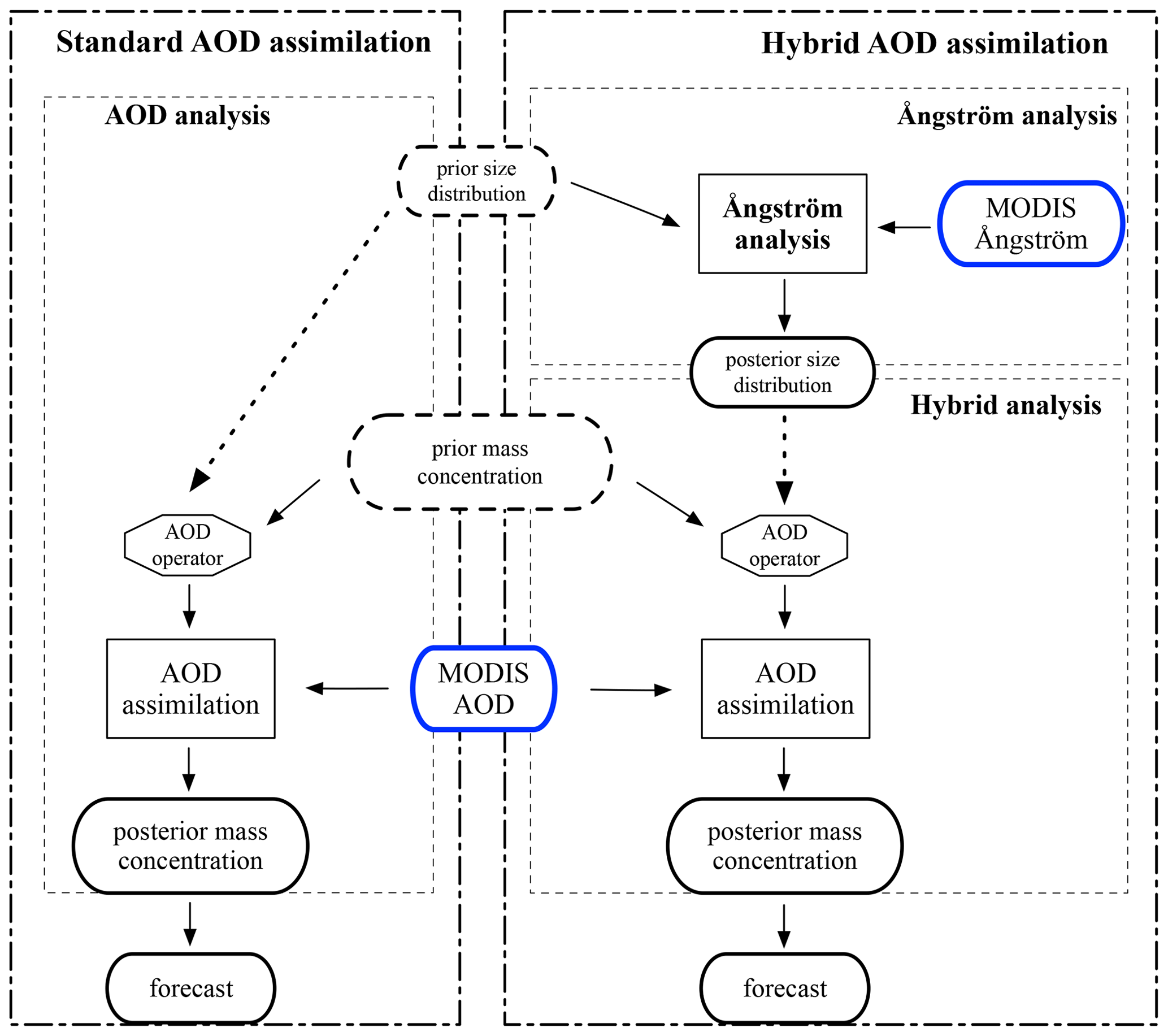
The data flow in the assimilation experiments is illustrated in Fig. 6. Two different assimilation configurations are distinguished: standard AOD assimilation that takes only AOD observations into account and the new hybrid AOD assimilation that also includes Ångström exponent observations. In both systems, the observations are used to obtain posterior aerosol mass concentrations that should better represent the actual concentrations. These could be used as initial conditions for a forecast, a simulation with a standard model configuration starting from the posterior concentrations; in this study, no forecast experiments are performed however. The assimilation of AOD observations is done in the same way in both systems; however, in the hybrid system, the assumed aerosol size distributions for the AOD simulations are obtained through an extra Ångström analysis. To distinguish the AOD assimilations from each other, the AOD assimilation using the AOD operator based on prior aerosol size distribution is referred to as the AOD analysis, while the AOD assimilation based on the posterior aerosol size distribution from the Ångström analysis is referred to as the hybrid analysis.

Both the AOD and hybrid assimilation methodologies will be applied to aerosol simulations over Europe from 23 to 26 July 2012. A single assimilation window of 4 d is used, collecting all available observations during the period and optimizing AOD or radii and AOD once. A systematic study with longer model periods and more assimilation cycles would help us to further understand temporal variation in the aerosol radius; this will be a part of our future work.

Figure 6 Standard and hybrid AOD data assimilation systems.

5.1.1 AOD assimilation methodology

The assimilation of AOD observations is performed using a 3D variational approach (Kalnay, 2002). The goal of the assimilation is to find posterior 3D aerosol concentrations X that provide the best simulation of AOD compared to the observations. In the variational approach, the optimal (analyzed) concentrations X_a are defined as an increment δX_a on the prior (or background) concentrations X_b:

$$\begin{array}{}\text{(6)}& {\mathit{X}}_{\mathrm{a}}={\mathit{X}}_{\mathrm{b}}+\mathit{\delta }{\mathit{X}}_{\mathrm{a}}.\end{array}$$

For simplicity (and computational efficiency) it is assumed that in the analyzed concentrations the ratios between different aerosol concentrations remain the same as in the background and that the vertical profile of the concentrations remains the same too. Under this assumptions it is sufficient to find an optimal 2D AOD field first and compute from that all 3D mass concentration increments. For this, first the AOD should be simulated from the background concentrations:

$$\begin{array}{}\text{(7)}& {\mathit{\tau }}_{\mathrm{b}}^{\mathrm{m}}=\mathcal{H}\left({\mathit{r}}_{\mathrm{b}}\right){\mathit{X}}_{\mathrm{b}}.\end{array}$$

Here, ℋ is the AOD observation operator that depends on the assumed aerosol size distribution parameters, which for the standard assimilation are the background or prior size distributions collected in r_b. In practice, ℋ represents the AOD simulation from the mass concentration in the model, as well as the observation selection operator. The latter is a matrix filled with 0/1 used for selecting the model AOD into the AOD observation space (white pixels excluded). To distinguish these two parts, we directly perform AOD assimilation analysis at pixels where AOD measurements are available. Hence, ℋ purely represents the conversion of aerosol mass concentration to AOD solely for this study.

The optimal (analyzed) AOD field ${\mathit{\tau }}_{\mathrm{a}}^{\mathrm{m}}$ is then defined as an increment of the background values:

$$\begin{array}{}\text{(8)}& {\mathit{\tau }}_{\mathrm{a}}^{\mathrm{m}}={\mathit{\tau }}_{\mathrm{b}}^{\mathrm{m}}+\mathit{\delta }{\mathit{\tau }}_{\mathrm{a}}^{\mathrm{m}}.\end{array}$$

When the optimal AOD increment $\mathit{\delta }{\mathit{\tau }}_{\mathrm{a}}^{\mathrm{m}}$ is found, the optimal concentration increment is calculated from

$$\begin{array}{}\text{(9)}& \mathit{\delta }{\mathit{X}}_{\mathrm{a}}(i,k,s)=\mathit{X}(i,k,s)\cdot {\displaystyle \frac{\mathit{\delta }{\mathit{\tau }}_{\mathrm{a}}^{\mathrm{m}}\left(i\right)}{{\mathit{\tau }}_{\mathrm{b}}^{\mathrm{m}}\left(i\right)}},\end{array}$$

where i and k denote the spatial and vertical location in the 3D model fields, and s denotes the aerosol tracer.

The optimal AOD increment $\mathit{\delta }{\mathit{\tau }}_{\mathrm{a}}^{\mathrm{m}}$ is defined as the field that minimizes the cost function:

$$\begin{array}{}\text{(10)}& \begin{array}{rl}J\left(\mathit{\delta }{\mathit{\tau }}_{\mathrm{a}}^{\mathrm{m}}\right)& ={\displaystyle \frac{\mathrm{1}}{\mathrm{2}}}\left(\mathit{\delta }{\mathit{\tau }}_{\mathrm{a}}^{\mathrm{m}}{)}^{\text{T}}{\mathbf{B}}_{\mathit{\tau }}^{-\mathrm{1}}\right(\mathit{\delta }{\mathit{\tau }}_{\mathrm{a}}^{\mathrm{m}})\\ & +{\displaystyle \frac{\mathrm{1}}{\mathrm{2}}}{\left({\mathit{\tau }}_{\mathrm{b}}^{\mathrm{m}}+\mathit{\delta }{\mathit{\tau }}_{\mathrm{a}}^{\mathrm{m}}-\mathit{\tau }\right)}^{\text{T}}{\mathbf{R}}_{\mathit{\tau }}^{-\mathrm{1}}\left({\mathit{\tau }}_{\mathrm{b}}^{\mathrm{m}}+\mathit{\delta }{\mathit{\tau }}_{\mathrm{a}}^{\mathrm{m}}-\mathit{\tau }\right).\end{array}\end{array}$$

The first part of the cost function defines a penalty on a perturbation from the background AOD. The background error covariance B_τ defines the weight of the penalty; how this covariance is defined is described below. The second part of the cost function defines a penalty on a deviation of the simulated AOD from the observations τ; the observation error covariance R_τ defines the weight of the penalty on an observation-minus-simulation mismatch.

The background and observation error covariance B_τ and R_τ together define the optimal solution of the minimization problem of Eq. (10) and are therefore the most important entities of the data assimilation system (Kalnay, 2002). In the background covariance B_τ, the main diagonal defines the assumed variance of the model AOD, while the offline elements represent the correlations between two AOD values in different grid cells. In this study the focus is on using the available AOD observations to obtain insight in the validity of the assumptions on the aerosol size distribution. Correlations between grid cells that would also influence the assimilation in practice are therefore simply ignored, and all optimizations are done per grid cell. The background covariance is therefore implemented as a diagonal matrix. We have used 30 % to characterize the uncertainty of our background AOD simulation, with a minimum uncertainty of 0.2 to prevent the posterior solution from becoming too close to the low-value AOD prior simulation:

$$\begin{array}{}\text{(11)}& {\mathbf{B}}_{\mathit{\tau }}(i,i)=\text{max}{\left(\mathrm{0.2},\mathrm{0.3}{\mathit{\tau }}_{\mathrm{b}}\left(i\right)\right)}^{\mathrm{2}}.\end{array}$$

The observation representation error covariance R_τ defines the errors in the observed AODs from instrument and retrieval uncertainties. These errors are assumed to be independent from each other, and therefore R_τ is modeled as a diagonal matrix. The diagonal elements are directly taken from the MODIS Deep Blue product.

5.1.2 Hybrid assimilation methodology

The hybrid assimilation is carried out by sequentially implementing the Ångström analysis and the AOD analysis. The Ångström assimilation focuses on estimating the aerosol size distribution and is performed through minimizing the following cost function:

$$\begin{array}{}\text{(12)}& \begin{array}{rl}J\left({\mathit{r}}_{\mathrm{a}}\right)& ={\displaystyle \frac{\mathrm{1}}{\mathrm{2}}}{\left({\mathit{r}}_{\mathrm{a}}-{\mathit{r}}_{\mathrm{b}}\right)}^{\text{T}}{\mathbf{B}}_{\mathit{r}}^{-\mathrm{1}}({\mathit{r}}_{\mathrm{a}}-{\mathit{r}}_{\mathrm{b}})\\ & +{\displaystyle \frac{\mathrm{1}}{\mathrm{2}}}{\left(\mathcal{M}\left({\mathit{r}}_{\mathrm{a}}\right){\mathit{X}}_{\mathrm{b}}-\mathcal{A}\right)}^{\text{T}}{\mathbf{R}}_{\mathcal{A}}^{-\mathrm{1}}\left(\mathcal{M}\left({\mathit{r}}_{\mathrm{a}}\right){\mathit{X}}_{\mathrm{b}}-\mathcal{A}\right).\end{array}\end{array}$$

The first part defines the mismatch between the optimal aerosol radius and the prior size assumptions, while the second part quantifies the penalty from the MODIS Ångström observations.

Vectors r_a and r_b denote the analyzed and prior aerosol radii over the 21 aerosol bins in Table 4. The aerosol radii are assumed to be spatially and temporally constant during the short period used for the experiments. Spatially varying radii would of course allow the assimilated Ångström exponent to better fit the MODIS Ångström exponent. However, the locally inconsistent MODIS Ångström observations found during comparison with AERONET observations in Sect. 3.2 would introduce strong local misadjustments in the case a (large) spatial degree of freedom is allowed. Data quality control for excluding these polluted data is required. Introducing spatial variations also requires information on spatial correlations and will increase computational costs; hence, this aspect has not been explored in this study. The radii of the different aerosol species are also assumed to be independent of each other. The background covariance matrix B_r is therefore diagonal, with elements set to the square of the uncertainties listed in Table 4. The uncertainties are chosen empirically and are capable of resolving the mismatch between the observed and simulated Ångström exponents.

During the test period, our LOTOS-EUROS simulated negligible dust levels. There were indeed some sea salt aerosols, but most of them stay over the ocean areas. This can be clearly seen in the snapshots of the column concentration of total fine aerosol, dust and sea salt in Fig. S6. However, our AOD assimilation was performed only in the MODIS Deep Blue observational space, as has been illustrated in Sect. 5.1.1, which only provides measurements over land areas. Therefore, both sea salt and dust aerosols have limited effects on our assimilation, and they are assumed to be certain and are not estimated in this study.

In the second part of the cost function Eq. (12), the operator ℳ(r_a) represents the Ångström simulation from the model state X_b, which depends on the aerosol size distribution r_a. Covariance matrix R_𝒜 defines the weight of the penalty for a mismatch between the simulation and the Ångström observation 𝒜. Similar to that for the AOD observation representation error, it is defined as a diagonal matrix under the assumption that all Ångström measurements are independent from each other. The diagonal elements are set to the square of 0.3, which is an empirical chosen value obtained from a comparison between the MODIS Ångström and AERONET Ångström measurements.

The aerosol radius r_a that minimizes the cost function Eq. (12) is obtained using a 4DvEnvar method (Liu et al., 2008), and the detailed procedures can be found in the Ångström analysis cost function minimization. An updated model AOD simulation is then obtained via

$$\begin{array}{}\text{(13)}& {\mathit{\tau }}_h^{\mathrm{m}}=\mathcal{H}\left({\mathit{r}}_{\mathrm{a}}\right)\mathit{X}.\end{array}$$

Following the same procedure as for the standard AOD assimilation, a new AOD analysis increment is obtained through the minimization of a cost function similar to Eq. (10):

$$\begin{array}{}\text{(14)}& \begin{array}{rl}J\left(\mathit{\delta }{\mathit{\tau }}_h^{\mathrm{m}}\right)& ={\displaystyle \frac{\mathrm{1}}{\mathrm{2}}}{\left(\mathit{\delta }{\mathit{\tau }}_h^{\mathrm{m}}\right)}^{\text{T}}{\mathbf{B}}_{\mathit{\tau }}^{-\mathrm{1}}\left(\mathit{\delta }{\mathit{\tau }}_h^{\mathrm{m}}\right)\\ & +{\displaystyle \frac{\mathrm{1}}{\mathrm{2}}}{\left({\mathit{\tau }}_h^{\mathrm{m}}+\mathit{\delta }{\mathit{\tau }}_h^{\mathrm{m}}-\mathit{\tau }\right)}^{\text{T}}{\mathbf{R}}_{\mathit{\tau }}^{-\mathrm{1}}\left({\mathit{\tau }}_h^{\mathrm{m}}+\mathit{\delta }{\mathit{\tau }}_h^{\mathrm{m}}-\mathit{\tau }\right).\end{array}\end{array}$$

With the optimal increments of AOD simulation δτ^m obtained through minimizing the above penal function (Eq. 14), the increments of aerosol mass concentration X can be calculated via

$$\begin{array}{}\text{(15)}& \mathit{\delta }{\mathit{X}}_h(i,k,s)=\mathit{X}(i,k,s)\cdot {\displaystyle \frac{\mathit{\delta }{\mathit{\tau }}_h^{\mathrm{m}}\left(i\right)}{{\mathit{\tau }}_h^{\mathrm{m}}\left(i\right)}}.\end{array}$$

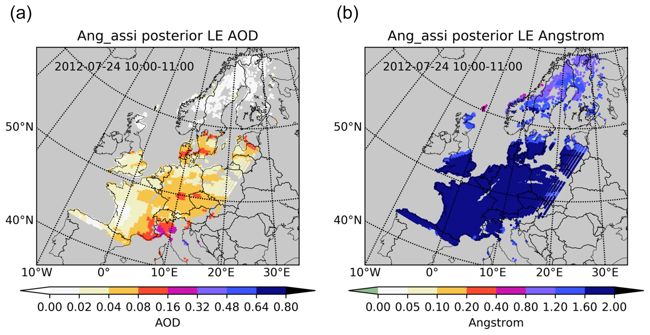
Figure 7 Posterior LOTOS-EUROS simulations of AOD (a) and Ångström exponent (b) on 24 July, 10:00 to 11:00 UTC after Ångström analysis.

5.2 Ångström analysis results

The Ångström analysis is performed first following the previously described methodology. The posterior radii of the 21 aerosol species are listed in Table 4. Compared to the prior assumptions, the Ångström analysis estimates smaller radii for the fine modes. The initial assumption of a geometric mean radius of 350 nm is reduced to about 90 nm for the inorganic aerosol in the fine mode, to 110 nm for black carbon, and 71 nm for organic and primary aerosols. The sizes assumed for the coarse mode are slightly increased from 2.5 µm initially to 2.7 µm for inorganic and black carbon aerosols, and they remain about the same for the organic and primary aerosols.

Before validating our optimized LOTOS-EUROS AOD operator, these posterior aerosol radii obtained through Ångström analysis are first compared to some aerosol size measurements. As shown in Table 5 there are several recent ground observations of aerosol lognormal size distribution over Europe. Compared to these observed radii, our prior assumption (0.35 µm) generally overestimated the fine aerosol size. The posterior geometric mean radii of the fine aerosols listed in Table 4 fall into the scope of most fine aerosol modes observed in Europe. However, as the documented aerosol size observations were collected in limited locations and different time periods, they cannot fully represent the true aerosol radii or assumptions in the satellite retrieval algorithm in our simulation. Further evaluation will be carried out using the AERONET optical measurements and ground PM_2.5 observations collected synchronously.

Costabile et al. (2009)Dall'Osto et al. (2019)Wu and Boor (2021)Rose et al. (2021)Leinonen et al. (2022)

Table 5 Summary of published observed lognormal size distribution parameters over Europe.

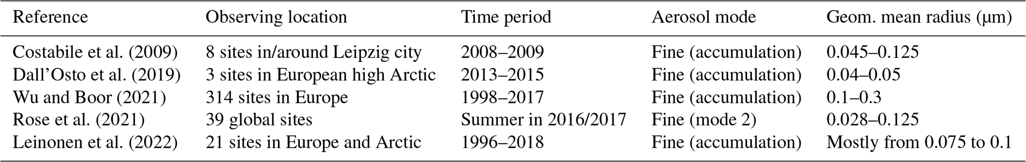
Figure 7 shows posterior simulations of AOD and the Ångström exponent using the optimized radii from the Ångström analysis. The simulated posterior Ångström exponents are now in the same range as the MODIS observations in Fig. 2b. Most of the values are in the range of 1.2 to 1.6, while the prior simulation produced negative values. The simulated Ångström exponent field is rather smooth since no spatial variation in the analysis was allowed. The AOD values simulated using the optimized radii (Fig. 7a) have increased compared to the prior simulation (Fig. 2c). The simulated AOD is however still underestimating the MODIS observations (Fig. 2a).

Time series of the posterior AOD and Ångström exponent simulations in the two AERONET sites of Cabauw and Leipzig are included in Figs. 3 and 4, respectively. Compared to the prior simulation, the posterior Ångström simulations are much closer to the independent AERONET observations. However, the temporal variability that is seen in the AERONET observations (blue dots) is not reproduced by the model. This could be explained by the use of aerosol radii that are constant in time. A temporally varying aerosol size is for the current application not feasible since it is based on MODIS data which have only a limited number of overpasses per day. The simulated AOD in the two sites is increased when using the posterior radii, but still an underestimation is present.

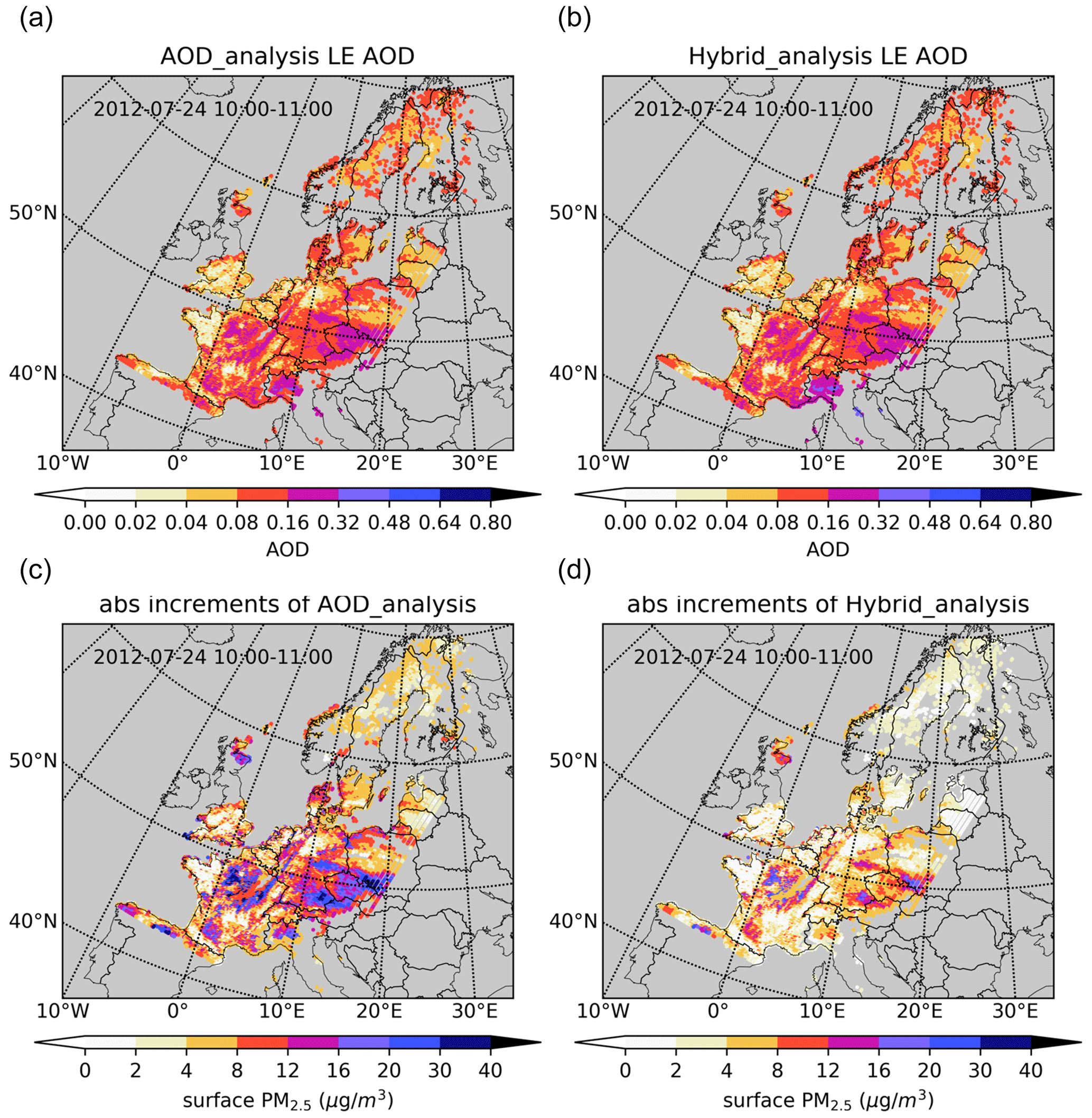
Figure 8 Posterior AOD simulations (a, b) and increments of surface PM_2.5 concentrations (c, d) in either AOD assimilation (a, c) or hybrid assimilation (b, d) on 24 July, 10:00 to 11:00 UTC.

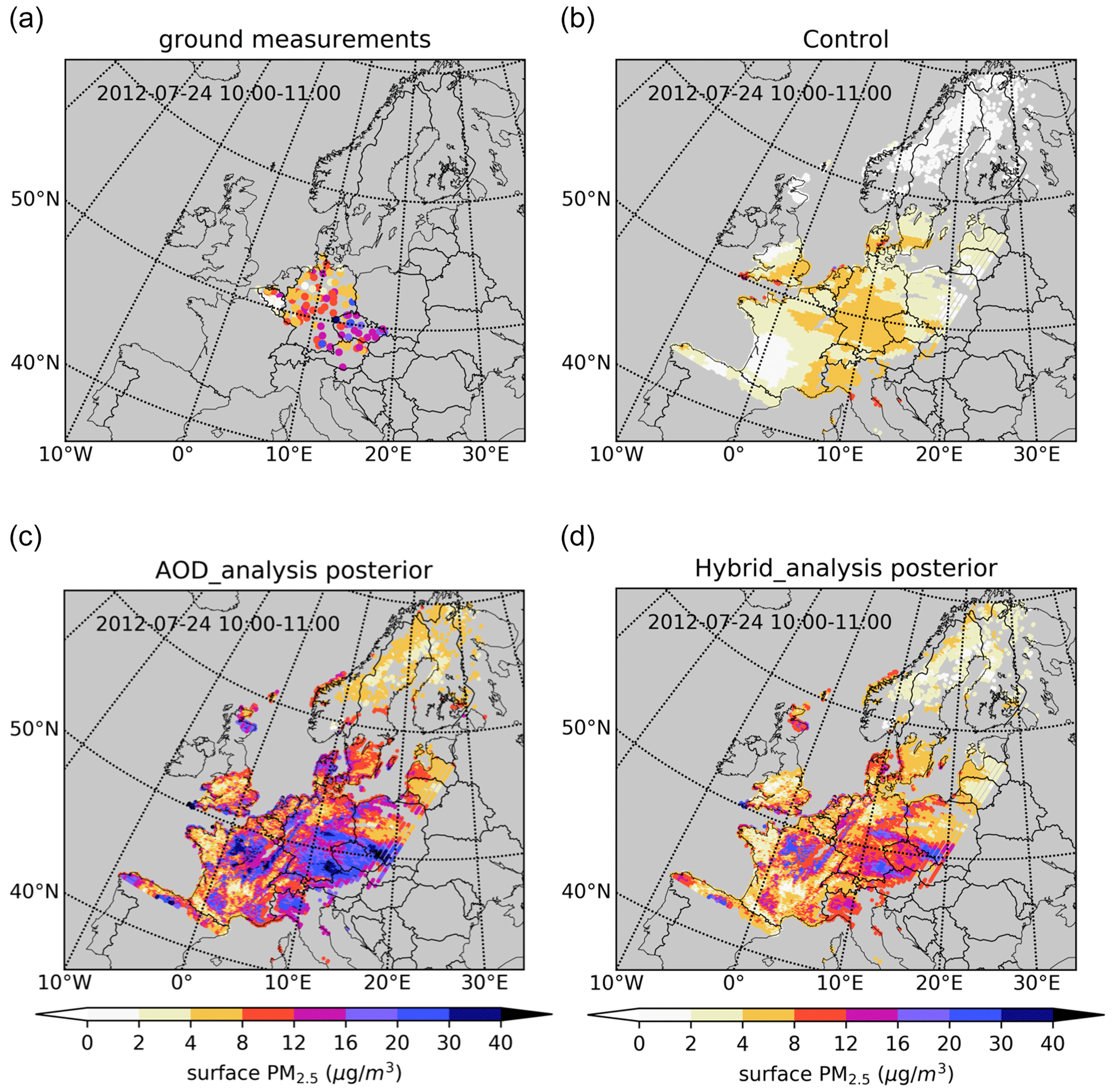
Figure 9 The surface PM_2.5 measurements (a), the simulations from the control run (b), the AOD analysis posterior (c) and the hybrid analysis posterior (d) on 24 July 2012 at 10:00–11:00 UTC.

5.3 AOD analysis results

Two assimilations of MODIS AOD have been performed either using the prior aerosol size distribution (AOD analysis) or using the posterior aerosol radius determined from the Ångström analysis (hybrid analysis). Figure 8a and b show examples of the posterior AOD simulations. Although the analyses are based on different prior AOD fields (see Figs. 2c and 7a), the posterior AOD values are very similar since they are optimized to represent the same MODIS AOD observations. However, the increments that were applied to the aerosol mass concentrations could be very different. The lower panels of Fig. 8 show the increment in surface PM_2.5 for the same hour as the AOD simulations in the upper panels. While in the AOD assimilation the increments range from 12 to 24 µg m⁻³, the increments in the hybrid assimilation are much lower and range from about 6 to 12 µg m⁻³. This shows that the AOD operator (or in this study, the assumed aerosol radii) strongly influences the aerosol mass concentration estimation during assimilations of AOD.

To evaluate the effect of the AOD and hybrid assimilation on aerosol concentrations, the posterior surface PM_2.5 simulations are compared to the ground PM_2.5 observations. Figure 9 shows maps of surface PM_2.5 measurements, as well as simulations from the control run, the AOD assimilation and the hybrid assimilation on 24 July (10:00–11:00 UTC). The PM_2.5 concentrations (Fig. 9a) are underestimated in the control run (Fig. 9b) but strongly increased by the assimilations (Fig. 9c and d). If only AOD is assimilated (Fig. 9c), the surface PM_2.5 concentrations actually exceed the observations. However, if aerosol radii are optimized first using the Ångström analysis in the hybrid assimilation, the simulated concentrations are in good agreement with the observations. This indicates that, although a standard AOD assimilation might be able to improve the AOD fields, it does not ensure the improvement on the aerosol mass concentration due to uncertainties in the AOD operator. The hybrid assimilation seems better able to relate AOD with aerosol masses since it uses aerosol sizes that are in better agreement with the retrieved Ångström exponent. It would be interesting to see whether the estimated radii are also in better agreement with the assumptions made in the aerosol retrieval algorithm.

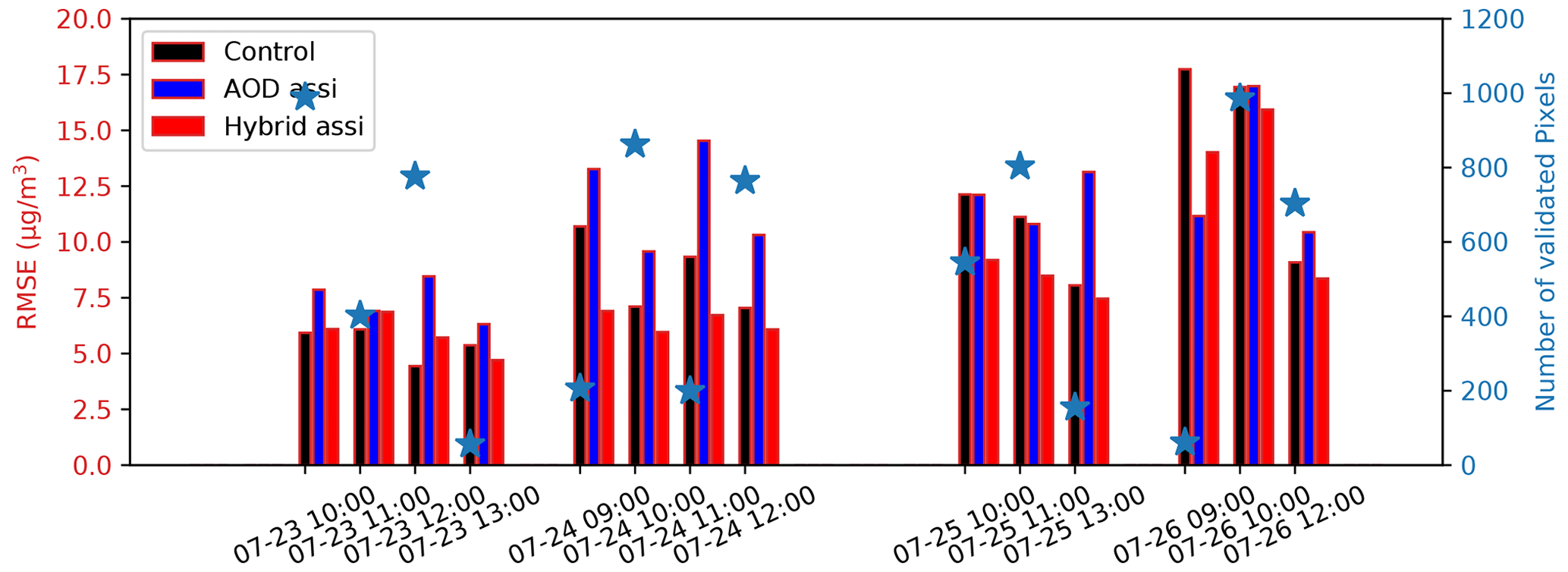
Figure 10 RMSE of the control, AOD analysis posterior (assi) and hybrid analysis posterior surface PM_2.5 level vs. the ground PM_2.5 measurements.

To further evaluate the impact of the Ångström analysis on PM_2.5 concentrations, the root mean square error (RMSE) between observations and simulations has been calculated for each of the hours for which MODIS observations were available in the 4 d window. The result is shown in Fig. 10, which also shows the number of MODIS observations available for analysis at each moment. For the control simulations the RMSE values are on average about 9 µg m⁻³. Assimilation of just the AOD observations actually increases the RMSE at most times, with an average value around 10.8 µg m⁻³; this indicates that the relation between aerosol mass and AOD is uncertain here. However, the hybrid assimilation is able to decrease the RMSE for almost all occasions to about 8.0 µg m⁻³.

6 Conclusions

In this study, we investigated the role of aerosol size distribution in calculating aerosol optical depth from aerosol mass concentrations in a simulation model. The assumptions on aerosol size distribution in the model should be in agreement with the assumptions made by the algorithms that retrieve AOD from remote sensing instruments. This is especially essential when remote sensing products such as AOD are assimilated in the model in order improve aerosol mass concentrations.

Aerosol extinction sensitivity tests based on an offline Mie code have been performed to test the relation between the aerosol size distribution and the extinction coefficients for different aerosol species (e.g., organic and inorganic carbon, black carbon, mineral dust, and sea salt aerosols) and for incident wavelengths. The results illustrated the high dependence of extinction coefficients on aerosol radii. However, the results also show that the Ångström exponent that is computed based on AOD at two different wavelengths is a suitable quantitative indicator of aerosol size. The Ångström exponents could therefore be used to improve the assumptions on aerosol size made in the simulation model.

To bring the retrieval and model AOD calculations in better agreement with each other using the Ångström exponent, a hybrid assimilation methodology is proposed. Different from a standard AOD assimilation that directly assimilates AOD observations and ignores the potential mismatch of the particle radius distribution, the hybrid approach first estimates optimal aerosol size parameters by assimilating Ångström exponent observations before performing the AOD analysis. In both the AOD and hybrid assimilation, the relative change in AOD obtained from the assimilation is used to scale aerosol mass concentrations. The proposed hybrid assimilation has been evaluated by assimilating MODIS Deep Blue AOD in a regional CTM over Europe during a 4 d assimilation window, preceded by an assimilation of corresponding Ångström exponents.

For the Ångström analysis that is part of the hybrid approach, validation with Ångström exponents retrieved from remote sensing observations from ground-based stations from the AERONET network showed strong improvement in simulated Ångström exponents. Since neither spatial nor temporal variation in aerosol radii was allowed in the experiments, fine-scale spatial and temporal variations could not be resolved yet. However, the first-order estimate of suitable aerosol radii is shown to be a useful improvement already and helps to avoid fine-scale inconsistencies in retrieved Ångström exponents having too strong an impact on results. It is advised that data selection procedures are applied on Ångström exponent observations before these are used in an assimilation.

Assimilations of AOD have been performed without and with a preceding analysis of Ångström exponents to optimize assumed aerosol radii. Both assimilations provide similar posterior AOD simulations since the same MODIS AOD observations are used; however, the assimilations provide different aerosol mass concentration. The posterior surface aerosol mass concentrations have been validated through a comparison with ground-based PM_2.5 measurements. In our 4 d test, the average RMSE of the simulations in the control run is about 9.3 µg m⁻³; when assimilating only AOD this actually increases to 10.8 µg m⁻³, which shows that a better AOD simulation does not necessarily imply a better aerosol mass representation. If in the hybrid assimilation Ångström exponents are also assimilated, the average RMSE decreases to 8.0 µg m⁻³.

The experiments show that for the assimilation of AOD observations with the goal of improving aerosol mass concentrations it is essential to take AOD at more than one wavelength into account, for example in the form of Ångström exponents. In this way it is possible to optimize the aerosol parameters that AOD simulations are sensitive to, such as the aerosol size that was the focus of this study. Further optimization of this and other parameters, including spatiotemporal variability in the aerosol size distribution and mass ratio of different aerosol species, will be the subject of future studies. A multiple-parameter optimization would benefit from extra observations, e.g., aerosol absorption optical depth, in addition to the currently used Ångström and AOD. With such a multi-observation assimilation it will be more possible to optimize aerosol mass concentrations including the different aerosol composition.