the Creative Commons Attribution 4.0 License.
the Creative Commons Attribution 4.0 License.
 | 01 Dec 2023
Long-term studies of the summer wind in the mesosphere and lower thermosphere at middle and high latitudes over Europe
Toralf Renkwitz
Huixin Liu
Christoph Jacobi
Robin Wing
Aleš Kuchař
Masaki Tsutsumi
Njål Gulbrandsen
Jorge L. Chau
Continuous wind measurements using partial-reflection radars and specular meteor radars have been carried out for nearly 2 decades (2004–2022) at middle and high latitudes over Germany (∼ 54° N) and northern Norway (∼ 69° N), respectively. They provide crucial data for understanding the long-term behavior of winds in the mesosphere and lower thermosphere. Our investigation focuses on the summer season, characterized by the low energy contribution from tides and relatively stable stratospheric conditions. This work presents the long-term behavior, variability, and trends of the maximum velocity of the summer eastward, westward, and southward winds. In addition, the geomagnetic influence on the summer zonal and meridional wind is explored at middle and high latitudes. The results show a mesospheric westward summer maximum located around 75 km with velocities of 35–54 m s−1, while the lower-thermospheric eastward wind maximum is observed at ∼ 97 km with wind speeds of 25–40 m s−1. A weaker southward wind peak is found around 86 km, ranging from 9 to 16 m s−1. The findings indicate significant trends at middle latitudes in the westward summer maxima with increasing winds over the past decades, while the southward winds show a decreasing trend. On the other hand, only the eastward wind in July has a decreasing trend at high latitudes. Evidence of oscillations around 2–3, 4, and 6 years modulate the maximum velocity of the summer winds. In particular, a periodicity between 10.2 and 11.3 years found in the westward component is more significant at middle latitudes than at high latitudes, possibly due to solar radiation. Furthermore, stronger geomagnetic activity at high latitudes causes an increase in eastward wind velocity, whereas the opposite effect is observed in zonal jets at middle latitudes. The meridional component appears to be disturbed during high geomagnetic activity, with a notable decrease in the northward wind strength below approximately 80 km at both latitudes.
- Article
(6304 KB) - Full-text XML
- BibTeX
- EndNote


The Earth's atmosphere constitutes a complex and dynamic system. The mesosphere and lower thermosphere (MLT) spanning between 50 and 110 km is a region where the neutral and ionized atmosphere coexist. The ionization process due to the absorption of solar irradiance governs the thermosphere, whereas the neutral atmosphere is subjected to active winds and wave interactions, leading to chemical mixing and temperature regulation. The stratosphere, which is located below the mesosphere, is the region where ozone mainly absorbs the ultraviolet (UV) radiation from the Sun.
In the 1980s, the ozone hole was discovered, which led to the awareness of health problems due to UV radiation. In 1987, the Montreal Protocol was implemented to stop the emission of ozone-depleting substances, and studies show a positive shift in the trends of stratospheric ozone in 1995 at equatorial latitudes and in 2000 at high latitudes (e.g., Weber et al., 2022). Since then, researchers have been studying long-term compositions, temperatures, and dynamics to understand the behavior of the atmosphere and the human footprint on the environment. Greenhouse gases, including CH4, H2O, O3, and CO2, are studied as tracers to monitor the evolution of the atmosphere (Bremer and Berger, 2002; Bremer and Peters, 2008; Yue et al., 2015; Peters and Entzian, 2015; Qian et al., 2017; Peters et al., 2017; Karagodin-Doyennel et al., 2021, etc.). At an altitude of 96 km, atomic oxygen is formed through the photo-dissociation of O2 and O3 in the mesopause. The atomic oxygen then interacts with CO2 through collisions, resulting in a radiative cooling effect that leads to hydrostatic contraction of the atmosphere (Gu et al., 2022; Akmaev, 2002; Li et al., 2021; Pisoft et al., 2021; Dawkins et al., 2023, etc.). As a consequence, carbon dioxide serves as a reliable indicator of cooling in the middle atmosphere, even during periods of disturbed geomagnetic activity (e.g., Liu et al., 2020).
The dynamics of the MLT are governed by the interaction of mean winds and waves, from large-scale planetary waves to small-scale gravity waves. The latter are driven by gravity and buoyancy in the atmosphere and are generated by orographic forcing, convection, wind shear, or wave interactions (Fritts and Alexander, 2003). Most gravity waves are generated in the troposphere and propagate upward and horizontally, breaking already in the troposphere and lower stratosphere. During winter, the zonal-mean zonal wind in the stratosphere and mesosphere is eastward and reverses in summer to be westward. The mean wind flow is crucial for the propagation of gravity waves. The linearized theory explains that gravity waves with an eastward velocity phase filtered by the westward wind reach the mesopause, where they break and deposit the momentum that decelerates the mean flow. This deceleration causes a wind reversal from westward to eastward in the summer lower thermosphere. As a consequence of the injection of energy from the breaking of the gravity waves and under the Coriolis force, a mean meridional circulation is induced from the summer hemisphere to the winter hemisphere, generating an upwelling in summer and a downwelling in winter. This circulation is the cause of the cold (warm) summer (winter) mesopause (Andrews et al., 1987; Holton and Alexander, 2000; Holton, 2004). In a non-linear regime, the contribution of anisotropic gravity waves has been proven to deposit a significant amount of momentum to the mean flow at lower altitudes (Medvedev et al., 1998). Furthermore, regions characterized by intense wind jets exhibit significant anisotropy, particularly in the upper area of a strong wind jet (Warner et al., 2005; Gong et al., 2008), which is a characteristic of the summer MLT. Additionally, the MLT exhibits sensitivity to external phenomena such as the stratospheric quasi-biennial oscillation (QBO), which alters the direction of the zonal winds over a span of 26–28 months, and the equatorial ocean–atmospheric warming (and cooling) that occurs during the Northern Hemisphere's winter season. This phenomenon, referred to as the El Niño–Southern Oscillation (ENSO), has periods that are not precisely defined but generally span around 3 to 6 years (Baldwin et al., 2001; Jacobi and Kürschner, 2002; Wang and Picaut, 2004; Espy et al., 2011; Offermann et al., 2015; French et al., 2020; Jaen et al., 2022).
Sprenger and Schminder (1969) studied the wind at 95 km during winter at middle latitudes and identified changes in the wind due to solar activity. The eastward component would reach 30–40 m s−1 during solar maximum but around 23 m s−1 during low solar activity. On the other hand, the meridional component shifted from 0 to 15 m s−1 in the southward direction during solar maximum and minimum, respectively. Later on, Bremer et al. (1997) identified weakly negative correlations with solar activity during most months (1964–1994) in the zonal component but with low significance, although the authors identified significant non-solar trends. Jacobi (1998) identified weaker eastward winds during solar maximum between 1972 and 1996. Portnyagin et al. (2006) studied the annual winds at middle latitudes between 1964 and 2004 and reported that zonal winds exhibited a decreasing trend, while meridional winds increased until 1980. However, after this time period, no significant trends were observed. The authors also identified different trends for the summer winds, specifically an increase in the summer zonal component in the 90s, as well as in the summer meridional component in the 70s, and concluded that these trends are non-uniform. Keuer et al. (2007) also found a correlation between solar activity and the MLT winds during summer, and the trend shows an increase in the zonal wind and a decrease in the meridional component during 1990–2005. Later on, Jacobi et al. (2015) reported an increase with weaker tendencies in the eastward winds, with a decrease in the southward component (1979–2014).
Hoffmann et al. (2010) compared 1 year of measurements from radars with the Kühlungsborn Mechanistic General Circulation Model (KMCM), showing the role of gravity wave drag in the summer MLT and the differences between middle and high latitudes and the interaction with waves between 12 and 72 h. Later on, Hoffmann et al. (2011) studied the long-term behavior of the winds and gravity wave activity from kinetic energy over Germany and Norway and showed differences between the intensity of these two. Particularly, they found trends in the westward wind increasing around 75 km and a corresponding increase in gravity wave activity of 3–6 h above 80 km (1990–2010) at middle latitudes, while this was not the behavior observed at high latitudes by Hibbins et al. (2007). Offermann et al. (2011) also identified trends in the eastward wind due to an increase in gravity waves at 87 km with hydroxyl (OH) measurements.
Considering all the mentioned studies, the MLT exhibits varying trends over time, with distinct behavior during winter and summer due to differences in the seasonal wind dynamics inherent to the wind field properties. Additionally, many studies have focused solely on wind velocities at fixed altitudes. However, as mentioned before, research suggests that the MLT height has been decreasing over the past decades (e.g., Peters et al., 2017; Vincent et al., 2019; Yuan et al., 2019; Dawkins et al., 2023). In light of this, the present study examines the maximum velocity of the horizontal winds independent of their altitude, their variability, and their trends over 19 years at high and middle latitudes over Europe during summer. In addition, the mesospheric time series at middle latitudes is extended to 33 years. Therefore, an introduction to the radar system and analysis methods implemented to extract the time series and analyze the trends is in Sect. 2. Section 3 describes the results obtained, while Sects. 4 and 5 provide the discussion and concluding remarks, respectively.
2.1 Radar observations
The observational data used in this work are entirely from two types of radars: partial-reflection radars (PRRs, also called MF radars) and specular meteor radars (SMRs). The PRR typically covers between 60 and 90 km altitude. Saura (69.14° N, 16.02° E) is located on Andøya, Norway, and has been in operation since 2004. This particular system operates with a peak power of 116 kW at a frequency of 3.17 MHz, having a Mills cross array that is composed of 29 crossed half-wave dipoles and thus offers a narrow beam for measurements (more information in Singer et al., 2005; Renkwitz and Latteck, 2017). A slightly smaller system which also has a Mills cross shape is located in Juliusruh (54.63° N 13.37° E), Germany, having an altitude coverage between 60 and 90 km. It has only 13 antennas and operates at a frequency of 3.18 MHz with a peak power of 64 kW. Starting as a frequency-modulated continuous wave radar in 1990, it was modernized into a modular pulsed system (more details on the Juliusruh PRR systems can be found in Keuer et al., 2007; Singer et al., 1992).
The SMRs use the plasma trails left by meteors disintegrating in the atmosphere to retrieve the MLT winds by measuring their position and Doppler shift (e.g., Hocking et al., 2001). These systems are capable of measuring winds between 70 and 110 km (depending on the number of meteor detections). Particularly for this work, we have combined detections from two closely located SMRs. This combination allows us to estimate the MLT mean winds, reducing data gaps and improving the precision and continuity of the time series. The latter is especially useful for long-term studies (e.g., Jaen et al., 2022).
At high latitudes, the Andenes SMR (69.27° N, 16.04° E) and Tromsø SMR (69.58° N, 19.22° E) are combined for measurements between 2004 and 2022, with a 4 km–4 h resolution to derive winds from 70 up to 110 km. In the case of middle latitudes, winds with 1 km–1 h resolution have been obtained by combining meteor detections from Collm SMR (51.3° N, 13.0° E) and Juliusruh SMR (54.63° N, 13.37° E), both operating in a pulsed mode. Note that both Andenes and Juliusruh SMR systems were upgraded in 2021 to operate in a coded continuous wave (CW) and multiple-input–multiple-output mode (e.g., Huyghebaert et al., 2022; Poblet et al., 2023, for details of the upgrades in Andenes and Juliusruh). In this work, measurements from only one receiving station located close to each coded-CW transmitter are used.
The SMR systems cover a volume spanning from a 250 km radius around a single system to 500 km or more, depending on the number of systems in the network. The winds used in the study are representative of the entire volume covered by the systems. While the SMR winds measure a larger volume than the PRR winds, the mean zonal wind is not affected by this difference in volume. However, the meridional wind presents a relatively larger latitudinal and longitudinal dependence, and these differences are more important. It has been studied and debated that PRRs underestimate the wind velocity above 80 km (Hall et al., 2005; Reid et al., 2018; Nozawa et al., 2002; Jacobi et al., 2009). Particularly for Saura PRR, the winds are corrected based on the angle of arrival statistics and compared to mesospheric very high frequency (VHF) wind measurements (Renkwitz et al., 2018).
2.2 Data analysis
In this study, most of the measurements have a length of 19 years (2004–2022), except for Juliusruh PRR with 33 years (1990–2022) at middle latitudes, from which we studied the mesospheric westward jet. To study the long-term behavior of the summer winds and their variability, we focus on the maximum median velocity per month as a proxy of the MLT dynamics. The different altitude ranges in the zonal and meridional data used for the climatologies aim to capture the maximum wind velocity. The zonal component is built with the combination of two datasets from different instruments, while the meridional component is only from SMRs since it captures the maximum wind velocity during summer. To obtain the time series, we calculated monthly median values and extracted the maximum velocity between a range of altitudes corresponding to the peak and latitude (i.e., westward jet: 65–96 km, southward wind: 75–95 km, and eastward jet: 80–106 km). With the maximum wind velocity per month v, we implemented a linear function to fit by least squares, , where m is the slope, yr is the year, and b is the v intercept. To test the slope of the linear fit, we implemented Student's t test to reject the null hypothesis () and calculated the confidence interval with 95 % confidence for the slope.
In order to study the variability of the time series, we implemented a generalized Lomb–Scargle (LS) periodogram analysis, with the difference between the 75 % and 25 % quartiles (third minus first) being an indication of the variability (since this is bigger than the measurements uncertainties), taken as the signal error (Czesla et al., 2019). The periodograms give the periods in years and the normalized power provided by PyAstronomy (Zechmeister and Kürster, 2009). With this implementation, it is possible to obtain the false-alarm probability (FAP) that responds to the question of what the probability is that a signal with no periodic component would lead to a peak of this magnitude over the highest peak, but it does not give information on the remaining peaks (VanderPlas, 2018). Even though the data are evenly spaced, one of the time series has a missing year (2000 in the Julisusruh PRR), which presents a complication in implementing the classical Fourier transform. In addition, Mossad et al. (2023) compared the Fourier transform to LS and found that LS is slightly more accurate for estimating the amplitude of a single frequency in the presence of minor gaps. The only disadvantage is the computation time, which, in this study, is not of importance given the number of data points.
It is widely known that there are many indices to categorize the atmosphere's external or internal forcing. In this case, we use the daily Ap index calculated from a network of magnetic observatories around the world. The Ap index varies between 0 and 400 and is the product of a conversion of the daily average of the 3 h mean Kp index (Matzka et al., 2021). Following the study at middle latitudes by Jacobi et al. (2021), we extend the work to 33 years below 82 km at middle latitudes and to high latitudes with the 19-year time series and investigate the response to disturbed and undisturbed geomagnetic conditions during summer. We divided the days of the years with low geomagnetic activity, Ap ≤5, and high geomagnetic activity, Ap ≥20, for middle latitudes and Ap ≥15 for high latitudes. The reason for the distinction comes from the nature of the behavior of the geomagnetic field with the change in latitudes. Juliusruh is located at 52° N geomagnetic latitude, while Andenes is located at 67° N. Renkwitz and Latteck (2017) showed that the majority of the particle precipitation events already occur at Kp =3 (Ap ≥15), which allows us to have a more robust time series considering the low geomagnetic activity in the last 19 years. In the case of middle latitudes, we use the limits already established by Jacobi et al. (2021). The time period used for the summer mean is 2004–2022, except for the zonal vertical profile (below 82 km) and the meridional profile (below 80 km) at middle latitudes, where the time period used is 1990–2022. Considering this selection, the total number of days between 2004 and 2022 is 888, 171, and 115 for Ap ≤5, Ap ≥15, and Ap ≥20, respectively. In the case of 1990–2022, it is 1228 (Ap ≤5) and 355 d (Ap ≥20)
The summer mean vertical wind profile is determined by utilizing the time series from the selected Ap index. The difference between high and low geomagnetic activity in the summer winds is computed, and then a Behrens–Fisher Student's t test is calculated since the variance hypothesis is not satisfied (i.e., the variances of the samples are not assumed to be equal), and a combined degree of freedom is calculated for this objective (Robinson, 1976).
3.1 Seasonal variations of winds
Figure 1a and b depict the climatologies of the mean zonal winds between 60 and 110 km at middle and high latitudes, respectively. The climatologies are the mean of all the years (2004–2021) after a 16 d smoothing window shifted by 1 d. The horizontal lines at 79.5 km at middle latitudes and at 85.5 km at high latitudes indicate the transition between the SMR and PRR measurements. Colors represent wind direction and intensity, while contour lines indicate wind velocity levels. Between January and March, the mean winds remain eastward until the springtime when the wind reversal occurs and the summertime begins (Jaen et al., 2022). During the summer months, the vertical wind profile (60–100 km) depicts the formation of the summer wind jets, with an increase in the wind velocity in May and reaching the maximum velocities between June and August (see Fig. 1a and b in blue). As a result of the eastward wind in the lower thermosphere and the westward wind in the mesosphere, a strong wind shear around 83–86 km at middle latitudes (87–90 km at high latitudes) is located at the mesopause. The intensity of the wind jets differs quantitatively: at middle latitudes, they are stronger than at high latitudes due to the mesospheric wind circulation. Below the zonal wind shear height and between 72 and 76 km (75 and 78 km), the westward wind velocity maxima reach a mean of approximately 54 m s−1 (45 m s−1). Above the strong wind shear and in the range of 93–98 km (97–100 km), the eastward jet mean is approximately 40 m s−1 (32 m s−1). As August progresses, the maximum velocity of the wind reduces, and by the end of the summer (middle of September), the wind reversal occurs below 85 km (88 km), leaving eastward wind during the winter in the MLT (Jaen et al., 2022).
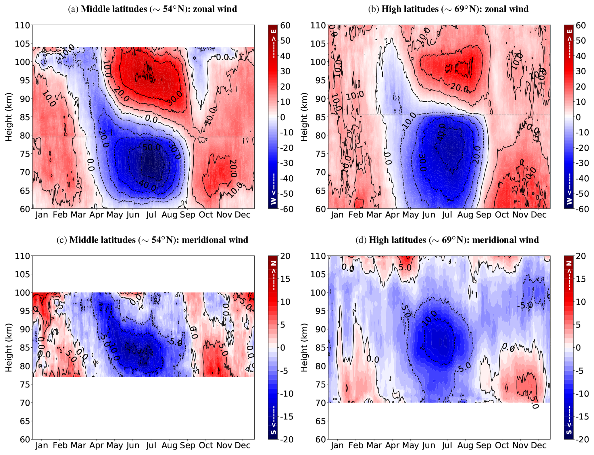
Figure 1Horizontal wind height–time cross-section of the annual variation at middle (a, c) and high (b, d) latitudes. The upper row depicts the zonal (a, b) component with eastward (red) and westward (blue) wind velocity (m s−1) by means of the color bar and the contour lines. The horizontal gray lines mark the change in the instrument. Similarly, the bottom row depicts the meridional component (c, d) with the northward (red) and southward (blue) wind velocity. Note that the meridional wind climatologies are only from SMR.
In terms of the meridional wind climatologies, Fig. 1c and d were obtained similarly to the zonal component, with the difference of using only the SMRs since the maximum summer wind altitude range is well captured by these radars. The meridional wind is less intense than the zonal wind. The velocity is quite variable in the observed range of 75–100 km. The velocity during the winter remains in the range of −5 to 5 m s−1. The time period between June and July depicts the strongest southward wind throughout the year and is located between 82 and 86 km at middle latitudes (85–89 km at high latitudes), with a median of 16 m s−1 (13 m s−1).
3.2 Trend in the horizontal winds
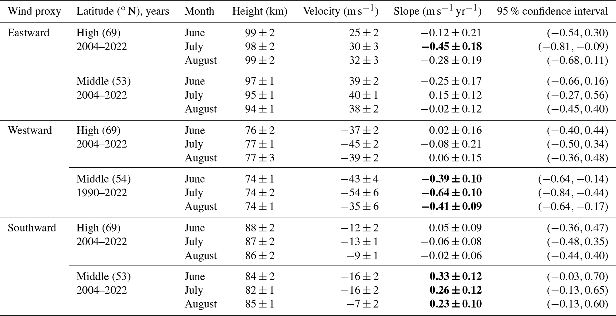
Figure 2 shows the time series peak velocity of the wind. Figure 2a and b are the eastward lower-thermospheric jets per year for June, July, and August (blue stars, red dots, and green triangles) at middle and high latitudes, respectively. For each time series, the shaded area represents the interval between the first and the third quartiles (25th and 75th empirical quartiles), and the linear fit is displayed in the corresponding color. Through the implementation of Student's t test and rejecting the null hypothesis (i.e., null slope, as discussed in Sect. 2.2), we obtain a statistical p value. The color lines are the possible trends where m is the slope, wherein a dashed colored line indicates a significance level exceeding 95 %. Conversely, a dotted line suggests that Student's t test did not reject the null hypothesis, implying that the slope could potentially be zero and thus that no significant trend exists. As a summary, the median height, the median velocity of the wind maxima, the slopes, and the 95 % confidence interval for the individual fit are listed in Table 1. In addition, the slopes with more than 95 % significance are highlighted in bold.
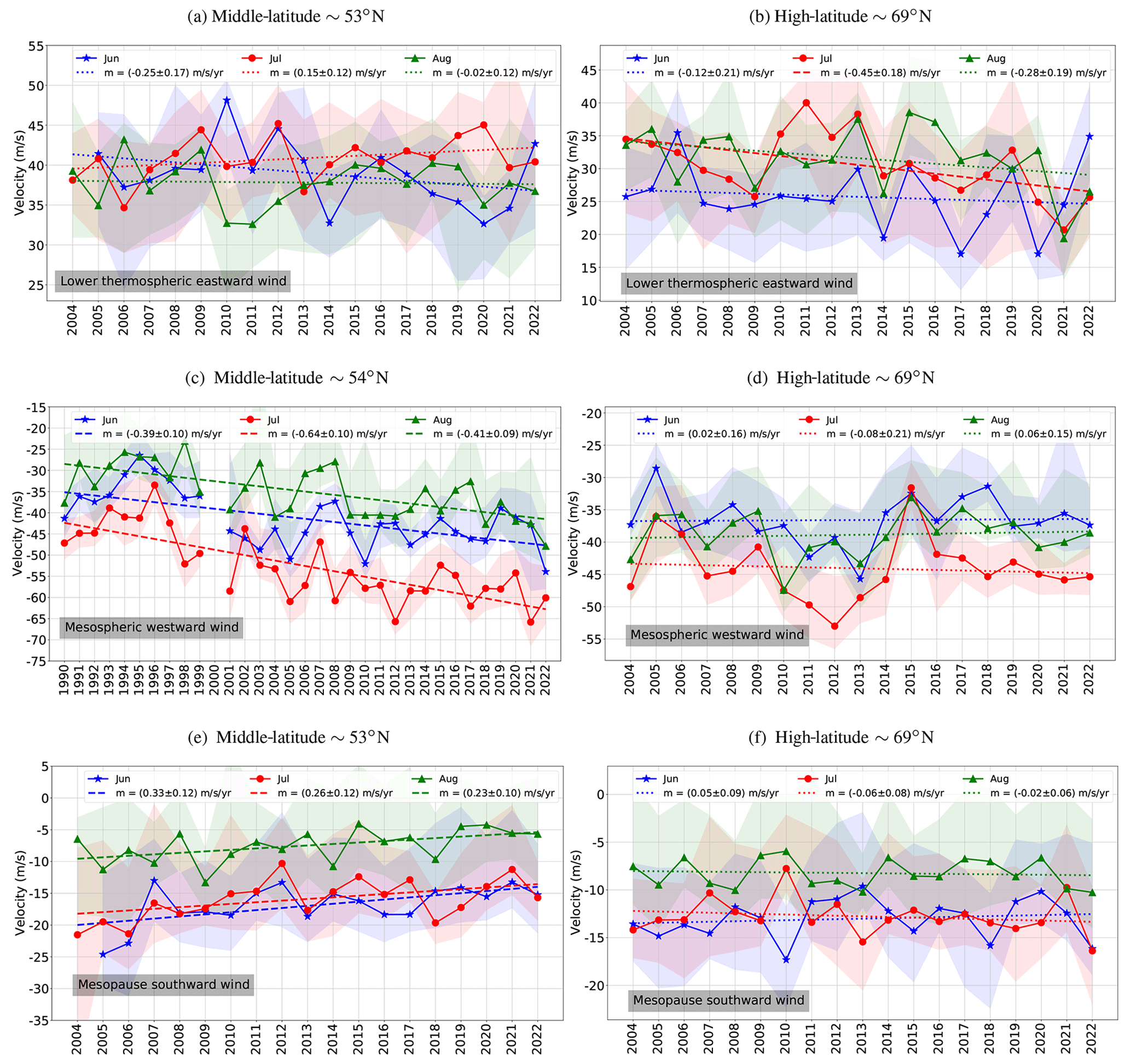
Figure 2Middle-latitude (a, c, e) and high-latitude (b, d, f) zonal and meridional wind maxima for every year. The eastward (a, b), westward (c, d), and southward (e, f) velocity maxima. Each wind component has the yearly velocity maxima obtained with a monthly median and their respective quartile difference (i.e., 75th and 25th quartiles). June (blue stars), July (red dots), and August (green triangles) with the linear fit where m represents the slope. The dashed lines depict the trends with 95 % significance.
Table 1Summary of the wind maxima characteristics with the respective latitude, the range of years, median height, median velocity, monthly slope with standard deviation, and the 95 % confidence interval. Highlighted in bold are the significant trends with more than 95 % confidence.
The eastward jets at middle latitudes (Fig. 2a) show no significant trends. However, at high latitudes, July depicts a significant trend with more than 98 % (see Fig. 2b), indicating weaker eastward winds over the years. In the case of the mesospheric westward jet at high latitudes, Student's t test does not reject the null-slope hypothesis, but the westward jet at middle latitudes depicts significant trends with more than 99.9 % for all the months, indicating a tendency for stronger westward winds since 1990 (Fig. 2c).
Figure 2e and f depict the southward winds at middle and high latitudes, respectively. In both cases, the jets are stronger during June and July than during August. While the southward maximum wind velocity remains approximately constant at high latitudes, at middle latitudes a significant trend (more than 95 % confidence) is visible, indicating a weakening of the meridional wind component over the years.
The altitude of the wind maxima fluctuates from year to year while consistently maintaining its mean height (see Table 1) without any significant trends between 2004 and 2022.
3.3 Interannual variability of winds
The time series in Fig. 2 reveals year-to-year variability, which motivated us to investigate the interannual variability of the time series through periodogram analyses. Figure 3 depicts the Lomb–Scargle periodograms of winds for each summer month. The upper row corresponds to middle latitudes, while the bottom row refers to high latitudes. The columns from left to right represent the lower-thermospheric eastward, mesospheric westward, and mesopause southward winds, respectively
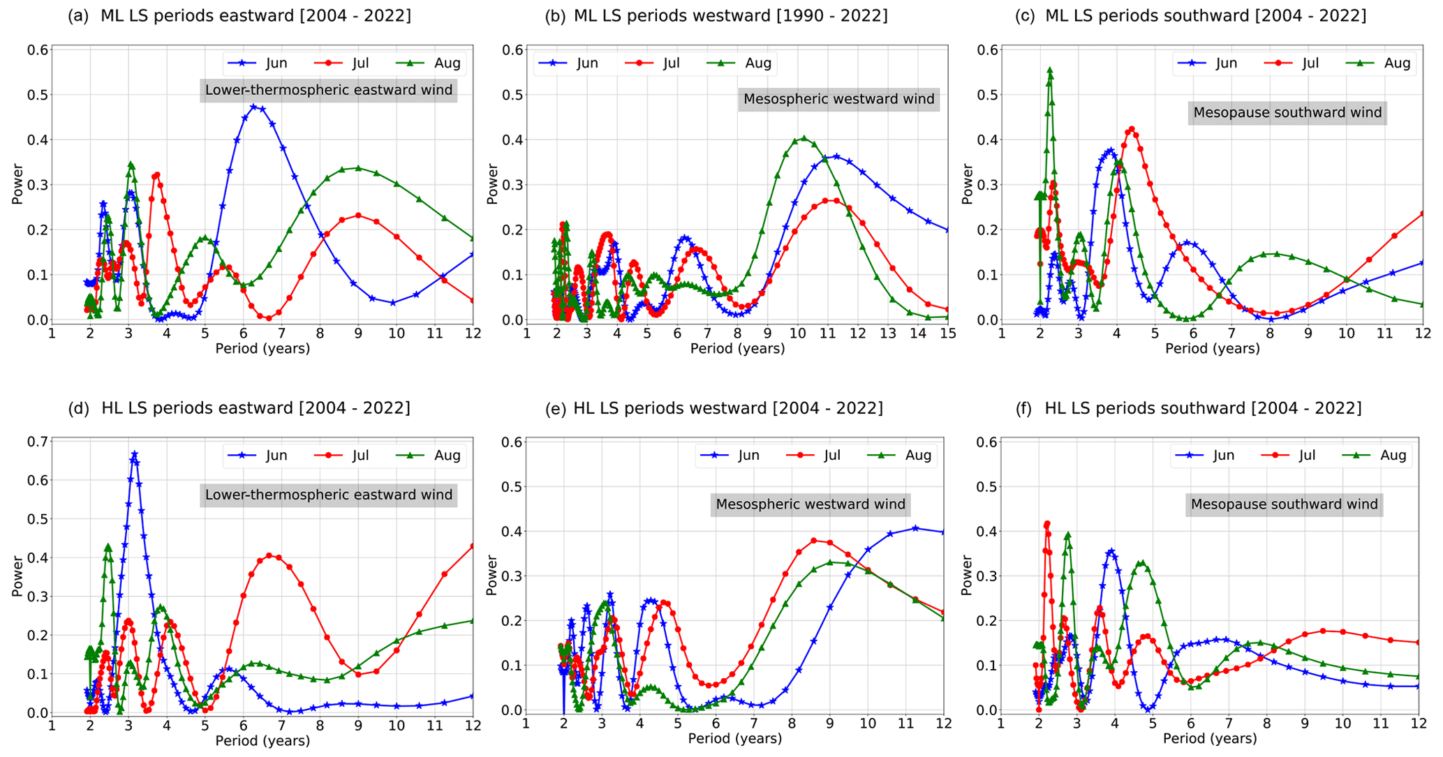
Figure 3Middle-latitude (a, b, c) and high-latitude (d, e, f) periodograms calculated with Lomb–Scargle. The left column represents the periodograms from the time series of the eastward maxima (a, d), the middle are the westward maxima (b, e), and the right column is the southward wind maxima (c, f).
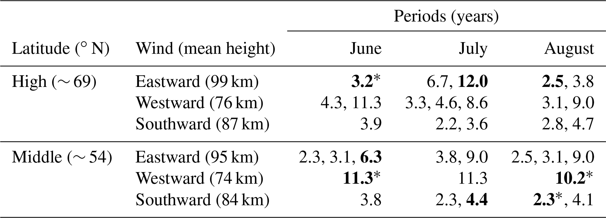
Table 2 summarizes the corresponding periods. At high latitudes, the eastward wind exhibits significant (over 90 % confidence level) periodicities of 2–3 years in June and August and of 12 years in July. At middle latitudes, significant periodicities are seen in the eastward wind around 6 years in June, in the westward wind around 10–11 years in June and August, and 2–4 years in the southward wind in July and August.
Table 2Summary of the periods obtained from LS analysis of monthly time series. The periods in bold are the ones that passed the false-alarm probability of 90 %, and the ones with a star are the ones that passed the false-alarm probability of 95 %.
3.4 Wind response to geomagnetic activity
Figure 4 shows the summer wind at high latitudes under quiet and disturbed geomagnetic conditions over the years. Figure 4a and b depict the yearly median summer zonal wind at low (Ap ≤5) and high (Ap ≥15) geomagnetic activity, respectively. On a simple visual examination, an enhancement in the eastward jet (red) under high geomagnetic activity is evident, while the westward jet (blue) remains in the same velocity range. The meridional component under disturbed geomagnetic conditions (Fig. 4d) displays a more variable velocity than at low geomagnetic activity (Fig. 4c). Note that, for high geomagnetic activity (Fig. 4b and d), the year 2020 depicts significant differences compared to the rest of the years due to the reduced number of days (2) with Ap ≥15.
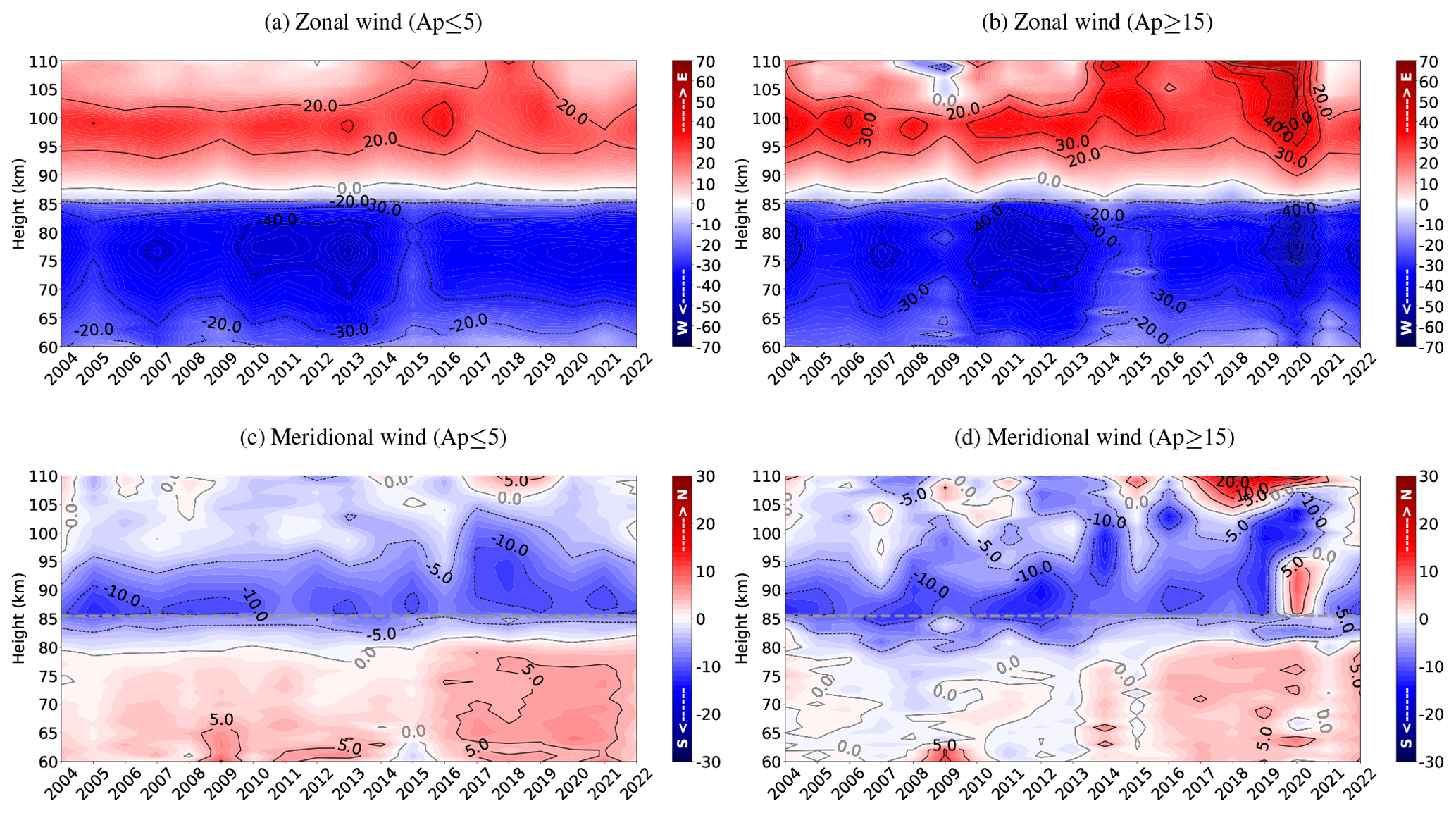
Figure 4Summer zonal winds at high latitudes over the years with low (a) and high (b) geomagnetic activity. In the same way, the bottom row depicts the summer meridional mean winds with low (c) and high (d) geomagnetic activity; this is also the case for high latitudes.
In order to quantify the possible differences, a summer mean with its standard deviation is calculated. The altitude velocity profiles for the summer mean at high latitudes are shown in Fig. 5 with low (green) and high (purple) geomagnetic activity for the zonal component (Fig. 5a) and the meridional component (Fig. 5b). They show stronger eastward winds under high geomagnetic activity above 92 km, while the rest of the profile does not exhibit a distinct difference between high and low geomagnetic activity.
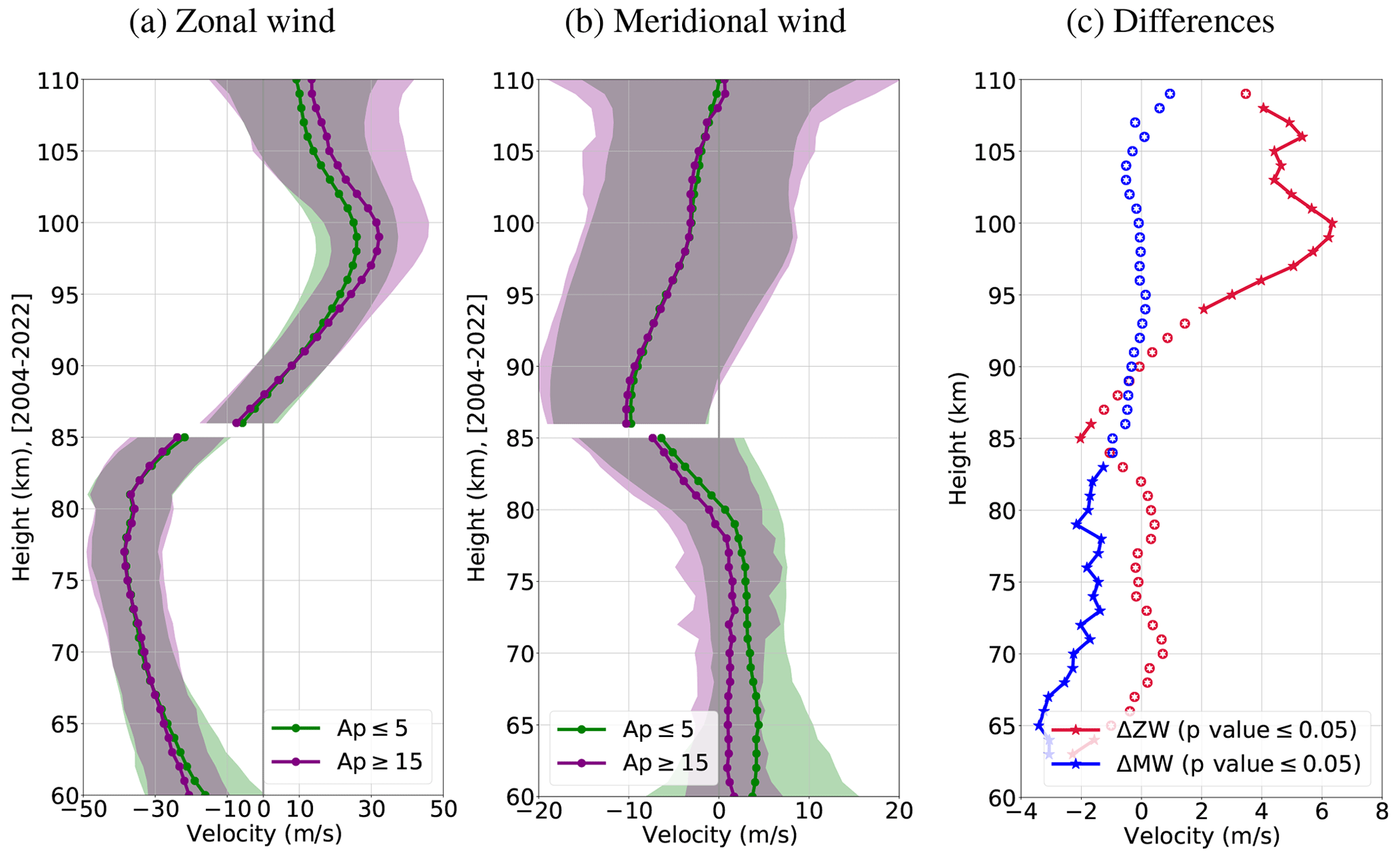
Figure 5Mean velocity profiles at high latitudes for low (green, Ap ≤5) and high (purple, Ap ≥15) geomagnetic activity for the summer zonal (a) and meridional (b) winds. The difference between both profiles under high and low geomagnetic activity (c) for the zonal (red) and the meridional (blue) wind component. The stars depict the values with more than 95 % significance, tested with the Behrens–Fisher test, and the circles the values with no significant difference between the means.
In the case of the meridional component (Fig. 5b), considerable differences appear below 85 km, with a stronger northward wind under quiet geomagnetic conditions. Figure 5c shows the difference between low and high geomagnetic activity for the zonal (red) and meridional (blue) summer wind components. Significant mean differences beyond 95 % according to the Behrens–Fisher test are denoted by stars, while circles indicate differences where the hypothesis of equal means was not rejected by the test. The summer eastward wind is significantly affected by geomagnetic activity, with 2–6 m s−1 stronger eastward wind velocities above 94 km and 1–3.5 m s−1 weaker northward winds below 83 km for strong geomagnetic activity.
A similar analysis is done for mid-latitudes, with the results shown in Fig. 6. Note that the zonal wind between 70 and 82 km and the meridional wind at 70–80 km are obtained between 1990 and 2022, while the winds above are obtained from 2004–2022 due to the use of different systems (see Sect. 2). The selection of the different range of altitudes or systems over the wind components is to avoid the instrument shift over the wind maxima, which is the focus of our study.
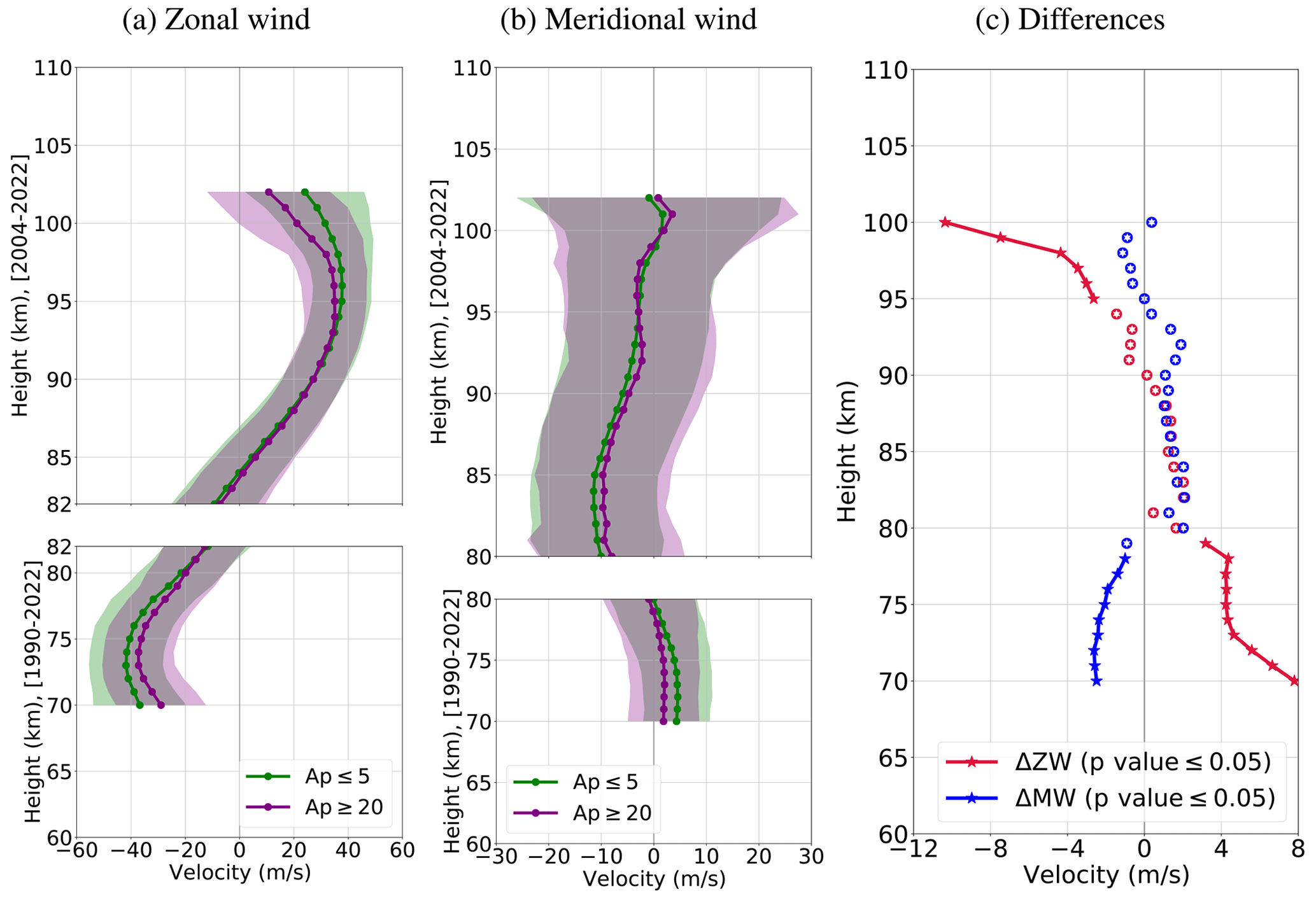
Figure 6Mean velocity profiles at middle latitudes for low (green, Ap ≤5) and high (purple, Ap ≥20) geomagnetic activity for the summer zonal (a) and meridional (b) winds. In the range of 70–82 (80) km, the zonal (meridional) components are calculated for the years 1990–2022. Above these heights, the analyzed years are 2004–2022. (c) The difference between both profiles under high and low geomagnetic activity for the zonal (red) and the meridional (blue) wind components. The stars depict the values with more than 95 % significance, tested with the Behrens–Fisher test, and the circles are the values with no significant difference between the means.
As shown in Fig. 6c, higher geomagnetic activity has a significant impact on the middle-latitude zonal wind, decelerating both the eastward jet (by up to −10 m s−1) above 95 km altitude and the westward jet below 80 km (by up to 8 m s−1). Its impact on the meridional wind is mainly seen below 78 km altitude, decelerating the northward wind by up to −3 m s−1. Note that there are differences between the meridional winds from Figs. 1d and 4c, d, which are a consequence of different instruments (see Sect. 2.1). Table 3 contains the trends calculated for July eastward and the summer westward maximum at high and middle latitudes, respectively, with only the days of low geomagnetic activity to compare with the significant trends in the zonal wind.
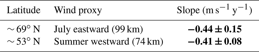
Table 3Wind maxima slopes obtained with the linear fit with days of low geomagnetic activity. Highlighted in bold are the significant trends with more than 95 % confidence.
In this work, we have explored the long-term variability of MLT summer wind using the maximum wind velocity as a proxy. The resulting time series were fitted with linear functions, and the slopes were tested in search of significant trends. In addition, we calculated the periodograms of the time series and explored the response of the wind under disturbed and non-disturbed geomagnetic conditions at high and middle latitudes.
4.1 Seasonal wind variations and trends
The wind climatologies are in agreement with previous studies at similar latitudes, considering the differences in height and investigated time lengths (Wilhelm et al., 2019; Hoffmann et al., 2010; Jaen et al., 2022; Schminder et al., 1997; Manson et al., 2004, etc.). However, a comparison with models shows that, in the summer season, WACCM-X(SD) and UA-ICON exhibit a good agreement with radars, while winter is better represented by GAIA (Ground-to-topside model of Atmosphere and Ionosphere for Aeronomy; Stober et al., 2021). Zhou et al. (2022) compared a network of meteor radars located at different latitudes (from middle to low latitudes) with WACCM-X(SD), finding similar results.
The wind trends observed in July for the lower-thermospheric eastward maxima at high latitudes and the southward maxima at middle latitudes are consistent with the study done by Wilhelm et al. (2019). In their work, the authors studied the trends at high latitudes and middle latitudes from 2002 to 2018 with specular meteor radars, and with this limitation, the westward wind maxima are not captured in their study, although a significant westward wind trend is visible below 85 km during the summer months. Hall and Tsutsumi (2013) made a similar study comparing two SMRs at latitudes of 70 and 78° N between 2001 and 2012. The authors identified a strengthening of the summer westward jet, contradicting our results. However, considering the time period during which their results overlap with those of our study (i.e., 2004–2012), it is visible in Fig. 2d that a possible significant trend could be found. On the other hand, Jacobi et al. (2023) analyzed 43 years of the winds near 90 and 81–85 km over Collm and Juliusruh, respectively, obtaining significant trends at Juliusruh for the summer-month eastward wind that do not agree with our findings. The differences can be attributed to the varying heights that were studied, which do not capture the proxies from this study. Hoffmann et al. (2011) studied the trends in the zonal wind for July at middle latitudes and found significant trends at 72 and 76 km, where the lower and upper limits of the westward jet are located. These trends showed stronger westward winds of 1.1 and 0.643 m s−1 yr−1, respectively, over the period of 1990–2010. Vincent et al. (2019) studied the trends in the meridional wind over the Antarctic (∼ 69° S) between 1994 and 2018 during the austral summer. While the study shows a descent in the height of the maximum wind velocity by 1.5 km, the strengths of the wind maxima did not change, which agrees with our findings in the Northern Hemisphere.
It is essential to highlight that, while the zonal wind shows a good representation of the global zonal wind behavior, the meridional component has a higher dependence on the region where it is observed, as a consequence of the gravity wave input at the mesopause (e.g., Jacobi et al., 2001). This could also explain the variations in trends across different latitudes and longitudes, as well as the limitations of global models, which often rely on parameterizations. Moreover, different lengths of the time series, their locations, and their parameters may show different trends due to the complex dynamics. Laštovička and Jelínek (2019) listed the main difficulties when studying trends.
4.2 Interannual oscillations
From the periodograms, several periods are identified (Fig. 3). Those periods of around 2–3 years could be associated with modulations from the stratospheric QBO, also called mesospheric QBO (MQBO). Espy et al. (2011) showed QBO modulation on the summer mesospheric OH temperatures at 60° N. The mesopause southward winds are a result of the eastward-phase gravity waves that reach the mesopause where they break and deposit momentum. Coupled with the Coriolis force, the meridional component of these winds drives the summer-to-winter pole circulation (e.g., Andrews et al., 1987; Holton, 2004). These gravity waves are previously filtered by the stratospheric flow, which is predominantly influenced by QBO (e.g., Baldwin et al., 2001; Lindzen and Holton, 1968). As such, these filtered gravity waves may be the underlying cause of the observed wind oscillations in the mesopause.
The periods between 3 and 4 years have been associated with modulation from ENSO. Reid et al. (2014) obtained oscillations of 3–4 years in OH and O (1 s) airglow at 96 and 87 km at 35° S. Perminov et al. (2018) obtained similar oscillations in OH temperatures at 56° N (2000–2016). García-Herrera et al. (2006) found a lag of a few months between ENSO and the temperature response in the stratosphere at high latitudes. Considering that ENSO's main phase occurs in December and the fact that it is an ocean–atmospheric event at equatorial latitudes, a signal's attenuation with time and space would be expected. While these findings are a result of mesospheric temperature observations, they are intrinsically linked to the mesospheric dynamics as expressed in the thermal-wind equation. Jacobi and Kürschner (2002) identified a possible signature of ENSO with Collm zonal winds in the 1980s and 1990s, and later on, Jacobi et al. (2017) found that this signal changes between the mesosphere and lower thermosphere. However, having common periodicity does not necessarily mean causality, and dedicated work needs to be done to connect these oscillations to QBO and ENSO phenomena.
4.3 Solar cycle dependence
The summer wind also shows a significant periodicity around 6 and 10–12 years, which could be a signature of the solar cycle and its harmonic (see Table 2). Previous works have shown connections between the solar cycle and the winds (e.g., Jacobi and Kürschner, 2006), while other authors have shown that these signatures have disappeared in past solar cycles (Portnyagin et al., 2006; Fiedler et al., 2011; DeLand and Thomas, 2015). For our data, a simple Pearson correlation between the Lyman α and the June westward wind maximum at middle latitudes gives , with a p value of 0.56, which indicates a non-significant anti-correlation. When considering the periods of 1990–2004 and 2004–2022 separately, we find two different correlations of (p value =0.01) and (p value =0.51), respectively. The first one shows a significant (≥95 %) anti-correlation between the westward wind maximum and Lyman α during the time length of 1990 to 2004, while the latter is not significant. Recently, Vellalassery et al. (2023) showed how the attenuation of the solar cycle response with Lyman α is correlated with the increase in water vapor in the mesosphere at polar latitudes.
4.4 Impact of geomagnetic activity on trends
Our results reveal an impact of geomagnetic activity on MLT winds in summer (Figs. 5 and 6), with higher geomagnetic activity weakening the winds at both middle and high latitudes, except for the eastward wind at high latitudes, which strengthens under disturbed conditions. The results at middle latitudes agree with those of Jacobi et al. (2021), who found weaker winds at a higher geomagnetic activity at two mid-latitude stations, Collm and Kazan, during the summers of 2016–2020.
Li et al. (2023, 2019) studied the response of the MLT during a geomagnetic storm with the thermosphere–ionosphere–mesosphere–electrodynamic general circulation model (TIMEGCM) at high and middle latitudes, respectively. While the effects of Joule heating penetrate up to ∼95 km at 70° N, the temperature contribution is minor compared to vertical heat advection and the adiabatic processes. Above 100 km, the Joule heating becomes significant and comparable to the other two processes. In the MLT, the major heating contributions are due to adiabatic heating and cooling and vertical heat advection associated with vertical winds. During a storm, the temperature increases and decreases with the vertical wind advection, and the horizontal advection also contributes to the total heating rate (Li et al., 2023). The meridional winds showed a shift in the direction, from southward to northward, similarly to the decrease in the winds observed below 79 km (Figs. 5b and 6b). These changes are a consequence of the temperature changes leading to downward or upward vertical winds which, together with the Coriolis force, produce a change in the pressure gradient (Li et al., 2019). However, Sun et al. (2022) compared the simulation with TIMEGCM and SABER (Sounding of the Atmosphere using Broadband Emission Radiometry) and found that the storm effects penetrate down to ∼ 80 km, and the model agrees with the observation but overestimates the temperature increase and underestimates the temperature decrease at high and middle latitudes.
The geomagnetic activity could significantly affect long-term trend studies, as demonstrated by Liu et al. (2021). Given the significant geomagnetic activity effect on the mesospheric wind, the long-term variation of the geomagnetic activity could potentially contribute to the wind trend we obtained in Fig. 2. The histogram in Fig. 7 shows the count of days from 1990 to 2022 with Ap ≤5 (green) and Ap ≥20 (purple). The right axis shows the scaled Lyman α (red line) to illustrate the solar activity over the investigated time period.
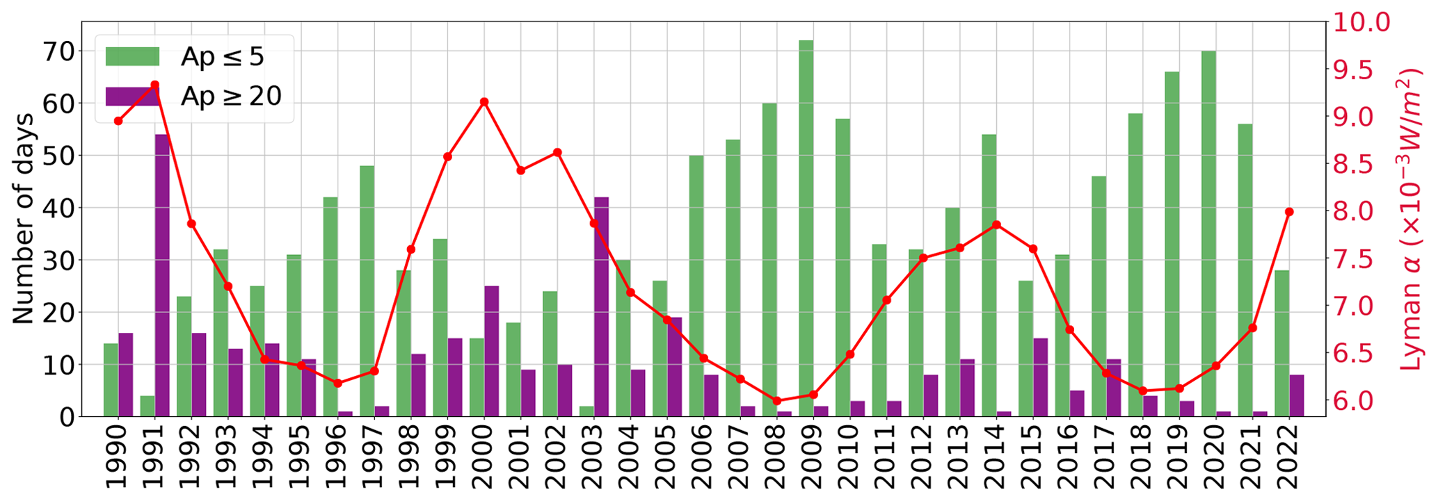
Figure 7Histogram with the counts of days for Ap ≤5 (green) and Ap ≥20 (purple). On the right axis is the Lyman α (red) scale with yearly summer mean values.
Comparatively, the first half of the time series has more days with high geomagnetic activity than the second half. This could imply that the negative trend in the westward jet can partially be due to more quiet days in the recent 2 decades. To test this, we calculated the summer mean (June–August averaged) maximum velocity from the yearly summer winds under only quiet conditions. At high latitudes, the eastward jet shows a significant summer trend of m s−1 yr−1 and a July eastward trend of m s−1 yr−1, in agreement with the complete time series (see Table 1). At middle latitudes, the westward jet also shows a significant trend of m s−1 yr−1, which is similar to the summer mean with the complete time series ( m s−1 yr−1). This result suggests that the winds are getting stronger due to different causes.
As to the cause of the long-term trends in the winds observed here, it could be related to changes in various atmospheric waves, such as planetary waves, tides, and gravity waves, as discussed by Laštovička et al. (2012). However, during summer, the contribution of tides is filtered at lower altitudes in the stratosphere, leaving less of a contribution in the mesosphere (Conte et al., 2017; Wilhelm et al., 2019; Pedatella et al., 2021). Ern et al. (2011) and Alexandre et al. (2021) found evidence of the fact that gravity waves generated in the lower latitudes of the summer hemisphere contribute to the momentum budget of the mesospheric jet in the middle and high latitudes. Hoffmann et al. (2011) found a significant trend of increasing gravity waves above 80 km. Liu et al. (2017) studied the gravity wave potential energy derived from satellite-observed temperatures and also found a positive trend below 80 km during July at 50° N. Furthermore, Luo et al. (2021) found a decreasing gravity wave trend in the stratosphere between 2007 and 2020, derived from temperature observations of GNSS radio occultation. A likely scenario could be a decrease in the stratospheric filtering of gravity waves, allowing them to reach higher altitudes and to deposit momentum flux in the mean westward flow (Medvedev et al., 1998; Yiğit and Medvedev, 2017; Conte et al., 2023). In a similar way, the southward wind is decreasing, and this could be a consequence of less energy reaching the mesopause due to the intense westward flow. In the future, we want to explore this possibility to identify the origin of this long-term trend.
The current paper examines long-term variations by analyzing the median maximum wind velocity in June, July, and August as an indicator of wind dynamics over the years. Linear functions were fitted to the time series, and the slope was tested using Student's t test; in addition, Lomb–Scargle periodograms were calculated. This study also investigates the relationship between wind patterns and geomagnetic activity by using the Ap index and tests its influence on the identified trends. The results are summarized as follows:
-
The lower-thermospheric eastward summer maximum in July shows a significant trend from 2004 to 2022 at high latitudes, with a decrease of (0.45±0.18) m s yr−1, exceeding 95 % statistical significance. The wind velocity reaches its peak between June and August, ranging from 25 to 32 m s−1 at an altitude of 98–99 km.
-
The mesospheric westward summer maximum has strengthened over the past 33 years (1990–2022) at middle latitudes. The highest velocity occurs in July, where it exhibits a significant trend of 0.64±0.10 m s−1. The summer mesospheric westward trends are independent of the geomagnetic activity.
-
The mesopause southward wind velocity experiences a significant decline during the 3 studied months at middle latitudes between 2004 and 2022, with the most substantial decrease occurring in June and July with slopes of 0.33±0.12 and 0.26±0.12 m s yr−1, respectively.
-
The summer mesospheric westward wind maxima exhibit an oscillation related to the solar cycle (8.6–11.3 years). This oscillation is significant for the months of June, July, and August during the period from 1990 to 2022. Additionally, other oscillations with periods of 2.3–2.8 and 3.2–4.4 years are present in most of the time series and could be associated with modulation from the QBO or ENSO.
-
Geomagnetic activity induces higher lower-thermospheric eastward winds above 94 km at high latitudes and weaker zonal winds at middle latitudes above 95 km and below 79 km.
-
The mesopause southward wind displays a disturbed pattern under high geomagnetic activity, reducing the wind velocity below 84 km at high latitudes and below 78 km at middle latitudes.
As the Earth's atmosphere continues evolving, the pursuit of long-term studies becomes increasingly challenging, yielding changing results over the years. Therefore, the acquisition of longer time series becomes imperative in order to truly comprehend the dynamics of the MLT. Although models have made notable improvements in their results, they still encounter certain limitations that need to be addressed. While measurements provide localized insights and show specific latitudinal characteristics, they inherently lack a comprehensive view of the entire system. Additionally, understanding the complexities of gravity waves in the middle atmosphere is crucial as they emerge as a significant energy source in the MLT dynamics.
The data to produce the figures are available in HDF5 format at https://doi.org/10.22000/1603 (Jaen, 2023).
JJ, TR, HL, and JC developed the idea and helped in the interpretation of results. NG and MT ensured the operation of the Tromsø specular meteor radar, and CJ ensured the operation of the Collm specular meteor radar. The writing of this paper was done by JJ with the assistance of all the authors, who made contributions to the discussion, draft review, and editing.
The contact author has declared that none of the authors has any competing interests.
Publisher’s note: Copernicus Publications remains neutral with regard to jurisdictional claims made in the text, published maps, institutional affiliations, or any other geographical representation in this paper. While Copernicus Publications makes every effort to include appropriate place names, the final responsibility lies with the authors.
This article is part of the special issue “Long-term changes and trends in the middle and upper atmosphere”. It is a result of the 11th International Workshop on Long-Term Changes and Trends in the Atmosphere, Helsinki, Finland, 23–27 May 2022.
Juliana Jaen thanks Axel Gabriel and Federico Conte for the helpful discussions and Matthias Clahsen for the data processing.
Lyman α is obtained from LISIRD (https://lasp.colorado.edu/lisird/, last access: 18 February 2023). Ap index is available from GFZ (https://www.gfz-potsdam.de/en/section/geomagnetism/data-products-services/geomagnetic-kp-index, last access: 25 November 2022).
The authors acknowledge the financial support of the Deutsche Forschungsgemeinschaft and the Bundesministerium für Bildung und Forschung (TIMA). Huixin Liu acknowledges the support of the JSPS KAKENHI and JRPs-LEAD with DFG.
This research has been supported by the Deutsche Forschungsgemeinschaft (grant nos. PO 2341/2-1, JA 836/47-1, and JPJSJPR 20181602), the Bundesministerium für Bildung und Forschung (grant no. 01 LG 1902A), and the Japan Society for the Promotion of Science (grant nos. 18H01270, 17KK0095, 20H00197, and 22K21345).
The publication of this article was funded by the Open Access Fund of the Leibniz Association.
This paper was edited by John Plane and reviewed by two anonymous referees.
Akmaev, R. A.: Modeling the cooling due to CO2 increases in the mesosphere and lower thermosphere, Phys. Chem. Earth, 27, 521–528, https://doi.org/10.1016/S1474-7065(02)00033-5, 2002. a
Alexandre, D., Thurairajah, B., England, S. L., and Cullens, C. Y.: A Hemispheric and Seasonal Comparison of Tropospheric to Mesospheric Gravity-Wave Propagation, J. Geophys. Res.-Atmos., 126, e2021JD034990, https://doi.org/10.1029/2021JD034990, 2021. a
Andrews, D. G., Holton, J. R., and Leovy, C. B.: Middle Atmosphere Dynamics, Vol. 40, 1st edn., Academic Press, ISBN: 0-12-058576-6, 1987. a, b
Baldwin, M. P., Gray, L. J., Dunkerton, T. J., Hamilton, K., Haynes, P. H., Randel, W. J., Holton, J. R., Alexander, M. J., Hirota, I., Horinouchi, T., Jones, D. B. A., Kinnersley, J. S., Marquardt, C., Sato, K., and Takahashi, M.: The quasi-biennial oscillation, Rev. Geophys., 39, 179–229, https://doi.org/10.1029/1999RG000073, 2001. a, b
Bremer, J. and Berger, U.: Mesospheric temperature trends derived from ground-based LF phase-height observations at mid-latitudes: Comparison with model simulations, J. Atmos. Sol.-Terr. Phy., 64, 805–816, https://doi.org/10.1016/S1364-6826(02)00073-1, 2002. a
Bremer, J. and Peters, D. H.: Influence of stratospheric ozone changes on long-term trends in the meso- and lower thermosphere, J. Atmos. Sol.-Terr. Phy., 70, 1473–1481, https://doi.org/10.1016/J.JASTP.2008.03.024, 2008. a
Bremer, J., Schminder, R., Greisiger, K. M., Hoffmann, P., Kürschner, D., and Singer, W.: Solar cycle dependence and long-term trends in the wind field of the mesosphere/lower thermosphere, J. Atmos. Sol.-Terr. Phy., 59, 497–509, https://doi.org/10.1016/S1364-6826(96)00032-6, 1997. a
Conte, J. F., Chau, J. L., Stober, G., Pedatella, N. M., Maute, A., Hoffmann, P., Janches, D., Fritts, D. C., and Murphy, D. J.: Climatology of semidiurnal lunar and solar tides at middle and high latitudes: Interhemispheric comparison, J. Geophys. Res.-Space, 122, 7750–7760, https://doi.org/10.1002/2017JA024396, 2017. a
Conte, J. F., Chau, J. L., Yigit, E., Suclupe, J., and Rodríguez, R. R.: Investigation of mesosphere and lower thermosphere dynamics over central and northern Peru using SIMONe systems, J. Geophys. Res.-Atmos., https://doi.org/10.1029/2009JD012388, 2023. a
Czesla, S., Schröter, S., Schneider, C. P., Huber, K. F., Pfeifer, F., Andreasen, D. T., and Zechmeister, M.: PyA: Python astronomy-related packages, https://ui.adsabs.harvard.edu/abs/2019ascl.soft06010C (last access: 23 April 2023), 2019. a
Dawkins, E. C. M., Stober, G., Janches, D., Carrillo‐Sánchez, J. D., Lieberman, R. S., Jacobi, C., Moffat‐Griffin, T., Mitchell, N. J., Cobbett, N., Batista, P. P., Andrioli, V. F., Buriti, R. A., Murphy, D. J., Kero, J., Gulbrandsen, N., Tsutsumi, M., Kozlovsky, A., Kim, J. H., Lee, C., and Lester, M.: Solar Cycle and Long‐Term Trends in the Observed Peak of the Meteor Altitude Distributions by Meteor Radars, Geophys. Res. Lett., 50, e2022GL101953, https://doi.org/10.1029/2022GL101953, 2023. a, b
DeLand, M. T. and Thomas, G. E.: Updated PMC trends derived from SBUV data, J. Geophys. Res.-Atmos., 120, 2140–2166, https://doi.org/10.1002/2014JD022253, 2015. a
Ern, M., Preusse, P., Gille, J. C., Hepplewhite, C. L., Mlynczak, M. G., Russell, J. M., and Riese, M.: Implications for atmospheric dynamics derived from global observations of gravity wave momentum flux in stratosphere and mesosphere, J. Geophys. Res.-Atmos., 116, D19107, https://doi.org/10.1029/2011JD015821, 2011. a
Espy, P. J., Ochoa Fernández, S., Forkman, P., Murtagh, D., and Stegman, J.: The role of the QBO in the inter-hemispheric coupling of summer mesospheric temperatures, Atmos. Chem. Phys., 11, 495–502, https://doi.org/10.5194/acp-11-495-2011, 2011. a, b
Fiedler, J., Baumgarten, G., Berger, U., Hoffmann, P., Kaifler, N., and Lübken, F.-J.: NLC and the background atmosphere above ALOMAR, Atmos. Chem. Phys., 11, 5701–5717, https://doi.org/10.5194/acp-11-5701-2011, 2011. a
French, W. J. R., Klekociuk, A. R., and Mulligan, F. J.: Analysis of 24 years of mesopause region OH rotational temperature observations at Davis, Antarctica – Part 2: Evidence of a quasi-quadrennial oscillation (QQO) in the polar mesosphere, Atmos. Chem. Phys., 20, 8691–8708, https://doi.org/10.5194/acp-20-8691-20200, 2020. a
Fritts, D. C. and Alexander, M. J.: Gravity wave dynamics and effects in the middle atmosphere, Rev. Geophys., 41, 1003, https://doi.org/10.1029/2001RG000106, 2003. a
García-Herrera, R., Calvo, N., Garcia, R. R., and Giorgetta, M. A.: Propagation of ENSO temperature signals into the middle atmosphere: A comparison of two general circulation models and ERA-40 reanalysis data, J. Geophys. Res. Atmos., 111, D06101, https://doi.org/10.1029/2005JD006061, 2006. a
Gong, J., Geller, M. A., and Wang, L.: Source spectra information derived from U.S. high-resolution radiosonde data, J. Geophys. Res., 113, D10106, https://doi.org/10.1029/2007JD009252, 2008. a
Gu, S., Zhao, H., Wei, Y., Wang, D., and Dou, X.: Atomic Oxygen SAO, AO and QBO in the Mesosphere and Lower Thermosphere Based on Measurements from SABER on TIMED during 2002–2019, Atmosphere, 13, 517, https://doi.org/10.3390/ATMOS13040517, 2022. a
Hall, C. M. and Tsutsumi, M.: Changes in mesospheric dynamics at 78° N, 16° E and 70° N, 19° E: 2001–2012, J. Geophys. Res.-Atmos., 118, 2689–2701, https://doi.org/10.1002/jgrd.50268, 2013. a
Hall, C. M., Aso, T., Tsutsumi, M., Nozawa, S., Manson, A. H., and Meek, C. E.: A comparison of mesosphere and lower thermosphere neutral winds as determined by meteor and medium-frequency radar at 70° N, Radio Sci., 40, RS4001, https://doi.org/10.1029/2004RS003102, 2005. a
Hibbins, R. E., Espy, P. J., Jarvis, M. J., Riggin, D. M., and Fritts, D. C.: A climatology of tides and gravity wave variance in the MLT above Rothera, Antarctica obtained by MF radar, J. Atmos. Sol.-Terr. Phy., 69, 578–588, https://doi.org/10.1016/J.JASTP.2006.10.009, 2007. a
Hocking, W. K., Fuller, R. A., and Vandepeer, B.: Real-time determination of meteor-related parameters utilizing modern digital technology, J. Atmos. Sol.-Terr. Phy., 63, 155–169, https://doi.org/10.1016/S1364-6826(00)00138-3, 2001. a
Hoffmann, P., Becker, E., Singer, W., and Placke, M.: Seasonal variation of mesospheric waves at northern middle and high latitudes, J. Atmos. Sol.-Terr. Phy., 72, 1068–1079, https://doi.org/10.1016/j.jastp.2010.07.002, 2010. a, b
Hoffmann, P., Rapp, M., Singer, W., and Keuer, D.: Trends of mesospheric gravity waves at northern middle latitudes during summer, J. Geophys. Res., 116, D00P08, https://doi.org/10.1029/2011JD015717, 2011. a, b, c
Holton, J. R.: An Introduction to Dynamic Meteorology, Elsevier, 4th edn., ISBN 0123540151, 2004. a, b
Holton, J. R. and Alexander, M. J.: The Role of Waves in the Transport Circulation of the Middle Atmosphere, Geoph. Monog. Series, 123, 161–176, https://doi.org/10.1029/GM123p0161, 2000. a
Huyghebaert, D., Clahsen, M., Chau, J. L., Renkwitz, T., Latteck, R., Johnsen, M. G., and Vierinen, J.: Multiple E-Region Radar Propagation Modes Measured by the VHF SIMONe Norway System During Active Ionospheric Conditions, Frontiers in Astronomy and Space Sciences, 9, 1–16, https://doi.org/10.3389/fspas.2022.886037, 2022. a
Jacobi, C.: On the solar cycle dependence of winds and planetary waves as seen from mid-latitude D1 LF mesopause region wind measurements, Ann. Geophys., 16, 1534–1543, https://doi.org/10.1007/s00585-998-1534-3, 1998. a
Jacobi, C. and Kürschner, D.: A possible connection of mid-latitude mesosphere/lower thermosphere zonal winds and the southern oscillation, Phys. Chem. Earth, 27, 571–577, https://doi.org/10.1016/S1474-7065(02)00039-6, 2002. a, b
Jacobi, C. and Kürschner, D.: Long-term trends of MLT region winds over Central Europe, Phys. Chem. Earth, 31, 16–21, https://doi.org/10.1016/j.pce.2005.01.004, 2006. a
Jacobi, C., Lange, M., Kürschner, D., Manson, A., and Meek, C.: A long-term comparison of saskatoon MF radar and collm LF D1 mesosphere-lower thermosphere wind measurements, Phys. Chem. Earth Pt. C, 26, 419–424, https://doi.org/10.1016/S1464-1917(01)00023-X, 2001. a
Jacobi, C., Arras, C., Kürschner, D., Singer, W., Hoffmann, P., and Keuer, D.: Comparison of mesopause region meteor radar winds, medium frequency radar winds and low frequency drifts over Germany, Adv. Space Res., 43, 247–252, https://doi.org/10.1016/j.asr.2008.05.009, 2009. a
Jacobi, C., Lilienthal, F., Geißler, C., and Krug, A.: Long-term variability of mid-latitude mesosphere-lower thermosphere winds over Collm (51° N, 13° E), J. Atmos. Sol.-Terr. Phy., 136, 174–186, https://doi.org/10.1016/j.jastp.2015.05.006, 2015. a
Jacobi, C., Krug, A., and Merzlyakov, E.: Radar observations of the quarterdiurnal tide at midlatitudes: Seasonal and long-term variations,J. Atmos. Sol.-Terr. Phy., 163, 70–77, https://doi.org/10.1016/j.jastp.2017.05.014, 2017. a
Jacobi, C., Lilienthal, F., Korotyshkin, D., Merzlyakov, E., and Stober, G.: Influence of geomagnetic disturbances on mean winds and tides in the mesosphere/lower thermosphere at midlatitudes, Adv. Radio Sci., 19, 185–193, https://doi.org/10.5194/ars-19-185-2021, 2021. a, b, c
Jacobi, C., Kuchar, A., Renkwitz, T., and Jaen, J.: Long-term trends of midlatitude horizontal mesosphere/lowerthermosphere winds over four decades, 2022 Kleinheubach Conference, KHB 2022, 1–11, https://doi.org/10.5194/ars-21-1-2023, 2023. a
Jaen, J.: JaenACP2023, Leibniz Institute of Atmospheric Physics at the University of Rostock [data set], https://doi.org/10.22000/1603, 2023. a
Jaen, J., Renkwitz, T., Chau, J. L., He, M., Hoffmann, P., Yamazaki, Y., Jacobi, C., Tsutsumi, M., Matthias, V., and Hall, C.: Long-term studies of mesosphere and lower-thermosphere summer length definitions based on mean zonal wind features observed for more than one solar cycle at middle and high latitudes in the Northern Hemisphere, Ann. Geophys., 40, 23–35, https://doi.org/10.5194/angeo-40-23-2022, 2022. a, b, c, d, e
Karagodin-Doyennel, A., Rozanov, E., Kuchar, A., Ball, W., Arsenovic, P., Remsberg, E., Jöckel, P., Kunze, M., Plummer, D. A., Stenke, A., Marsh, D., Kinnison, D., and Peter, T.: The response of mesospheric H2O and CO to solar irradiance variability in models and observations, Atmos. Chem. Phys., 21, 201–216, https://doi.org/10.5194/acp-21-201-2021, 2021. a
Keuer, D., Hoffmann, P., Singer, W., and Bremer, J.: Long-term variations of the mesospheric wind field at mid-latitudes, Ann. Geophys., 25, 1779–1790, https://doi.org/10.5194/angeo-25-1779-2007, 2007. a, b
Laštovička, J. and Jelínek, Š.: Problems in calculating long-term trends in the upper atmosphere, J. Atmos. Sol.-Terr. Phy., 189, 80–86, https://doi.org/10.1016/j.jastp.2019.04.011, 2019. a
Laštovička, J., Solomon, S. C., and Qian, L.: Trends in the Neutral and Ionized Upper Atmosphere, Space Sci. Rev., 168, 113–145, https://doi.org/10.1007/s11214-011-9799-3, 2012. a
Li, J., Wang, W., Lu, J., Yue, J., Burns, A. G., Yuan, T., Chen, X., and Dong, W.: A Modeling Study of the Responses of Mesosphere and Lower Thermosphere Winds to Geomagnetic Storms at Middle Latitudes, J. Geophys. Res.-Space, 124, 3666–3680, https://doi.org/10.1029/2019JA026533, 2019. a, b
Li, J., Wei, G., Wang, W., Luo, Q., Lu, J., Tian, Y., Xiong, S., Sun, M., Shen, F., Yuan, T., Zhang, X., Fu, S., Li, Z., Zhang, H., and Yang, C.: A Modeling Study on the Responses of the Mesosphere and Lower Thermosphere (MLT) Temperature to the Initial and Main Phases of Geomagnetic Storms at High Latitudes, J. Geophys. Res.-Atmos., 128, 1–14, https://doi.org/10.1029/2022JD038348, 2023. a, b
Li, T., Yue, J., Russell, J. M., and Zhang, X.: Long-term trend and solar cycle in the middle atmosphere temperature revealed from merged HALOE and SABER datasets, J. Atmos. Sol.-Terr. Phy., 212, 105506, https://doi.org/10.1016/J.JASTP.2020.105506, 2021. a
Lindzen, R. S. and Holton, J. R.: A Theory of the Quasi-Biennial Oscillation, J. Atmos. Sci., 25, 1095–1107, https://doi.org/10.1175/1520-0469(1968)025<1095:ATOTQB>2.0.CO;2, 1968. a
Liu, H., Tao, C., Jin, H., and Nakamoto, Y.: Circulation and Tides in a Cooler Upper Atmosphere: Dynamical Effects of CO2 Doubling, Geophys. Res. Lett., 47, 1–9, https://doi.org/10.1029/2020GL087413, 2020. a
Liu, H., Tao, C., Jin, H., and Abe, T.: Geomagnetic activity effects on CO2-driven trend in the thermosphere and ionosphere: ideal model experiments with GAIA, J. Geophys. Res.-Space, 126, e2020JA028607, https://doi.org/10.1029/2020JA028607, 2021. a
Liu, X., Yue, J., Xu, J., Garcia, R. R., Russell, J. M., Mlynczak, M., Wu, D. L., and Nakamura, T.: Variations of global gravity waves derived from 14 years of SABER temperature observations, J. Geophys. Res., 122, 6231–6249, https://doi.org/10.1002/2017JD026604, 2017. a
Luo, J., Hou, J., and Xu, X.: Variations in stratospheric gravity waves derived from temperature observations of multi-gnss radio occultation missions, Remote Sensing, 13, 1–20, https://doi.org/10.3390/rs13234835, 2021. a
Manson, A. H., Meek, C. E., Hall, C. M., Nozawa, S., Mitchell, N. J., Pancheva, D., Singer, W., and Hoffmann, P.: Mesopause dynamics from the scandinavian triangle of radars within the PSMOS-DATAR Project, Ann. Geophys., 22, 367–386, https://doi.org/10.5194/angeo-22-367-2004, 2004. a
Matzka, J., Stolle, C., Yamazaki, Y., Bronkalla, O., and Morschhauser, A.: The Geomagnetic Kp Index and Derived Indices of Geomagnetic Activity, Space Weather, 19, e2020SW002641, https://doi.org/10.1029/2020SW002641, 2021. a
Medvedev, A. S., Klaassen, G. P., and Beagley, S. R.: On the role of an anisotropic gravity wave spectrum in maintaining the circulation of the middle atmosphere, Geophys. Res. Lett., 25, 509–512, https://doi.org/10.1029/98GL50177, 1998. a, b
Mossad, M., Strelnikova, I., Wing, R., and Baumgarten, G.: Assessing Atmospheric Gravity Wave Spectra in the Presence of Observational Gaps, EGUsphere [preprint], https://doi.org/10.5194/egusphere-2023-1598, 2023. a
Nozawa, S., Brekke, A., Manson, A., Hall, C. M., Meek, C., Morise, K., Oyama, S., Dobashi, K., and Fujii, R.: A comparison study of the auroral lower thermospheric neutral winds derived by the EISCAT UHF radar and the Tromso medium frequency radar, J. Geophys. Res.-Space, 107, SIA 29-1–SIA 29-20, https://doi.org/10.1029/2000JA007581, 2002. a
Offermann, D., Hoffmann, P., Knieling, P., Koppmann, R., Oberheide, J., Riggin, D. M., Tunbridge, V. M., and Steinbrecht, W.: Quasi 2 day waves in the summer mesosphere: Triple structure of amplitudes and long-term development, J. Geophys. Res., 116, D00P02, https://doi.org/10.1029/2010JD015051, 2011. a
Offermann, D., Goussev, O., Kalicinsky, C., Koppmann, R., Matthes, K., Schmidt, H., Steinbrecht, W., and Wintel, J.: A case study of multi-annual temperature oscillations in the atmosphere: Middle Europe, J. Atmos. Sol.-Terr. Phy., 135, 1–11, https://doi.org/10.1016/j.jastp.2015.10.003, 2015. a
Pedatella, N. M., Liu, H. L., Conte, J. F., Chau, J. L., Hall, C., Jacobi, C., Mitchell, N., and Tsutsumi, M.: Migrating Semidiurnal Tide During the September Equinox Transition in the Northern Hemisphere, J. Geophys. Res.-Atmos., 126, 1–14, https://doi.org/10.1029/2020JD033822, 2021. a
Perminov, V., Semenov, A., Pertsev, N., Medvedeva, I., Dalin, P., and Sukhodoev, V.: Multi-year behaviour of the midnight OH* temperature according to observations at Zvenigorod over 2000–2016, Adv. Space Res., 61, 1901–1908, https://doi.org/10.1016/j.asr.2017.07.020, 2018. a
Peters, D. H. and Entzian, G.: Long-term variability of 50 years of standard phase-height measurement at Kühlungsborn, Mecklenburg, Germany, Adv. Space Res., 55, 1764–1774, https://doi.org/10.1016/j.asr.2015.01.021, 2015. a
Peters, D. H., Entzian, G., and Keckhut, P.: Mesospheric temperature trends derived from standard phase-height measurements, J. Atmos. Sol.-Terr. Phy., 163, 23–30, https://doi.org/10.1016/j.jastp.2017.04.007, 2017. a, b
Pisoft, P., Sacha, P., Polvani, L. M., Añel, J. A., de la Torre, L., Eichinger, R., Foelsche, U., Huszar, P., Jacobi, C., Karlicky, J., Kuchar, A., Miksovsky, J., Zak, M., and Rieder, H. E.: Stratospheric contraction caused by increasing greenhouse gases, Environ. Res. Lett., 16, 064038, https://doi.org/10.1088/1748-9326/abfe2b, 2021. a
Poblet, F. L., Vierinen, J., Avsarkisov, V., Conte, J. F., Charuvil Asokan, H., Jacobi, C., and Chau, J. L.: Horizontal Correlation Functions of Wind Fluctuations in the Mesosphere and Lower Thermosphere, J. Geophys. Res.-Atmos., 128, e2022JD038092, https://doi.org/10.1029/2022JD038092, 2023. a
Portnyagin, Y. I., Merzlyakov, E. G., Solovjova, T. V., Jacobi, C., Kürschner, D., Manson, A. H., and Meek, C.: Long-term trends and year-to-year variability of mid-latitude mesosphere/lower thermosphere winds, J. Atmos. Sol.-Terr. Phy., 68, 1890–1901, https://doi.org/10.1016/j.jastp.2006.04.004, 2006. a, b
Qian, L., Burns, A. G., Solomon, S. C., and Wang, W.: Carbon dioxide trends in the mesosphere and lower thermosphere, J. Geophys. Res.-Space, 122, 4474–4488, https://doi.org/10.1002/2016JA023825, 2017. a
Reid, I. M., Spargo, A. J., and Woithe, J. M.: Seasonal variations of the nighttime O(1S) and OH (8-3) airglow intensity at Adelaide, Australia, J. Geophys. Res., 119, 6991–7013, https://doi.org/10.1002/2013JD020906, 2014. a
Reid, I. M., McIntosh, D. L., Murphy, D. J., and Vincent, R. A.: Mesospheric radar wind comparisons at high and middle southern latitudes, Earth Planets Space, 70, 1–16, https://doi.org/10.1186/s40623-018-0861-1, 2018. a
Renkwitz, T. and Latteck, R.: Variability of virtual layered phenomena in the mesosphere observed with medium frequency radars at 69° N, J. Atmos. Sol.-Terr. Phy., 163, 38–45, https://doi.org/10.1016/j.jastp.2017.05.009, 2017. a, b
Renkwitz, T., Tsutsumi, M., Laskar, F. I., Chau, J. L., and Latteck, R.: On the role of anisotropic MF/HF scattering in mesospheric wind estimation, Earth Planets Space, 70, 158, https://doi.org/10.1186/s40623-018-0927-0, 2018. a
Robinson, G. K.: Properties of student's t and of the Behrens-Fisher solution to the two means problem, Ann. Stat., 4, 963–971, https://doi.org/10.1214/aos/1176343594, 1976. a
Schminder, R., Kürschner, D., Singer, W., Hoffmann, P., Keuer, D., and Bremer, J.: Representative height-time cross-sections of the upper atmosphere wind field over Central Europe 1990-1996, J. Atmos. Sol.-Terr. Phy., 59, 2177–2184, https://doi.org/10.1016/S1364-6826(97)00062-X, 1997. a
Singer, W., Hoffmann, P., Keuer, D., Schminder, R., and Kuerschner, D.: Wind in the middle atmosphere with partial reflection measurements during winter and spring in middle europe, Adv. Space Res., 12, 299–302, https://doi.org/10.1016/0273-1177(92)90483-E, 1992. a
Singer, W., Latteck, R., Friedrich, M., Dalin, P., Kirkwood, S., Engler, N., and Holdsworth, D. A.: D-region electron densities obtained by differential absorption and phase measurements with a 3-MHz-Doppler radar, in: 17th ESA Symposium on European Rocket and Balloon Programmes and Related Research, Sandefjord, Norway, 30 May–2 June 2005, 233–238, ISBN 9783540773405, 2005. a
Sprenger, K. and Schminder, R.: Solar cycle dependence of winds in the lower ionosphere, J. Atmos. Terr. Phys., 31, 217–221, https://doi.org/10.1016/0021-9169(69)90100-7, 1969. a
Stober, G., Kuchar, A., Pokhotelov, D., Liu, H., Liu, H.-L., Schmidt, H., Jacobi, C., Baumgarten, K., Brown, P., Janches, D., Murphy, D., Kozlovsky, A., Lester, M., Belova, E., Kero, J., and Mitchell, N.: Interhemispheric differences of mesosphere–lower thermosphere winds and tides investigated from three whole-atmosphere models and meteor radar observations, Atmos. Chem. Phys., 21, 13855–13902, https://doi.org/10.5194/acp-21-13855-2021, 2021. a
Sun, M., Li, Z., Li, J., Lu, J., Gu, C., Zhu, M., and Tian, Y.: Responses of Mesosphere and Lower Thermosphere Temperature to the Geomagnetic Storm on 7–8 September 2017, Universe, 8, 96, https://doi.org/10.3390/universe8020096, 2022. a
VanderPlas, J. T.: Understanding the Lomb–Scargle Periodogram, Astrophys. J. Suppl. S., 236, 16, https://doi.org/10.3847/1538-4365/AAB766, 2018. a
Vellalassery, A., Baumgarten, G., Grygalashvyly, M., and Lübken, F.-J.: Greenhouse gas effects on the solar cycle response of water vapour and noctilucent clouds, Ann. Geophys., 41, 289–300, https://doi.org/10.5194/angeo-41-289-2023, 2023. a
Vincent, R. A., Kovalam, S., Murphy, D. J., Reid, I. M., and Younger, J. P.: Trends and Variability in Vertical Winds in the Southern Hemisphere Summer Polar Mesosphere and Lower Thermosphere, J. Geophys. Res.-Atmos., 124, 11070–11085, https://doi.org/10.1029/2019JD030735, 2019. a, b
Wang, C. and Picaut, J.: Understanding ENSO physics–a review, Geoph. Monog. Series, 147, 21–48, https://doi.org/10.1029/147GM02, 2004. a
Warner, C. D., Scaife, A. A., and Butchart, N.: Filtering of parameterized nonorographic gravity waves in the Met Office Unified Model, J. Atmos. Sci., 62, 1831–1848, https://doi.org/10.1175/JAS3450.1, 2005. a
Weber, M., Arosio, C., Coldewey-Egbers, M., Fioletov, V. E., Frith, S. M., Wild, J. D., Tourpali, K., Burrows, J. P., and Loyola, D.: Global total ozone recovery trends attributed to ozone-depleting substance (ODS) changes derived from five merged ozone datasets, Atmos. Chem. Phys., 22, 6843–6859, https://doi.org/10.5194/acp-22-6843-2022, 2022. a
Wilhelm, S., Stober, G., and Brown, P.: Climatologies and long-term changes in mesospheric wind and wave measurements based on radar observations at high and mid latitudes, Ann. Geophys., 37, 851–875, https://doi.org/10.5194/angeo-37-851-2019, 2019. a, b, c
Yiğit, E. and Medvedev, A. S.: Influence of parameterized small-scale gravity waves on the migrating diurnal tide in Earth's thermosphere, J. Geophys. Res.-Space, 122, 4846–4864, https://doi.org/10.1002/2017JA024089, 2017. a
Yuan, T., Solomon, S. C., She, C.-Y. Y., Krueger, D. A., and Liu, H.-L. H. L.: The Long‐Term Trends of Nocturnal Mesopause Temperature and Altitude Revealed by Na Lidar Observations Between 1990 and 2018 at Midlatitude, J. Geophys. Res.-Atmos., 124, 5970–5980, https://doi.org/10.1029/2018JD029828, 2019. a
Yue, J., Russell, J., Jian, Y., Rezac, L., Garcia, R., López-Puertas, M., and Mlynczak, M. G.: Increasing carbon dioxide concentration in the upper atmosphere observed by SABER, Geophys. Res. Lett., 42, 7194–7199, https://doi.org/10.1002/2015GL064696, 2015. a
Zechmeister, M. and Kürster, M.: The generalised Lomb-Scargle periodogram, Astron. Astrophys., 496, 577–584, https://doi.org/10.1051/0004-6361:200811296, 2009. a
Zhou, B., Xue, X., Yi, W., Ye, H., Zeng, J., Chen, J., Wu, J., Chen, T., and Dou, X.: A comparison of MLT wind between meteor radar chain data and SD-WACCM results, Earth and Planetary Physics, 6, 451–464, https://doi.org/10.26464/epp2022040, 2022. a