the Creative Commons Attribution 4.0 License.
the Creative Commons Attribution 4.0 License.
 | 24 Nov 2023
Two years of satellite-based carbon dioxide emission quantification at the world's largest coal-fired power plants
Andrew K. Thorpe
Charles E. Miller
Alana K. Ayasse
Ralph Jiorle
Riley M. Duren
Ray Nassar
Jon-Paul Mastrogiacomo
Robert R. Nelson
Carbon dioxide (CO2) emissions from combustion sources are uncertain in many places across the globe. Satellites have the ability to detect and quantify emissions from large CO2 point sources, including coal-fired power plants. In this study, we routinely made observations with the PRecursore IperSpettrale della Missione Applicativa (PRISMA) satellite imaging spectrometer and the Orbiting Carbon Observatory-3 (OCO-3) instrument aboard the International Space Station at over 30 coal-fired power plants between 2021 and 2022. CO2 plumes were detected in 50 % of the acquired PRISMA scenes, which is consistent with the combined influence of viewing parameters on detection (solar illumination and surface reflectance) and unknown factors (e.g., daily operational status). We compare satellite-derived emission rates to in situ stack emission observations and find average agreement to within 27 % for PRISMA and 30 % for OCO-3, although more observations are needed to robustly characterize the error. We highlight two examples of fusing PRISMA with OCO-2 and OCO-3 observations in South Africa and India. For India, we acquired PRISMA and OCO-3 observations on the same day and used the high-spatial-resolution capability of PRISMA (30 m spatial/pixel resolution) to partition relative contributions of two distinct emitting power plants to the net emission. Although an encouraging start, 2 years of observations from these satellites did not produce sufficient observations to estimate annual average emission rates within low (<15 %) uncertainties. However, as the constellation of CO2-observing satellites is poised to significantly improve in the coming decade, this study offers an approach to leverage multiple observation platforms to better quantify and characterize uncertainty for large anthropogenic emission sources.
- Article
(7033 KB) - Full-text XML
- BibTeX
- EndNote


The works published in this journal are distributed under the Creative Commons Attribution 4.0 License. This license does not affect the Crown copyright work, which is re-usable under the Open Government Licence (OGL). The Creative Commons Attribution 4.0 License and the OGL are interoperable and do not conflict with, reduce or limit each other.
© Crown copyright 2023
Anthropogenic carbon dioxide (CO2) emissions are dominated by strong discrete point sources: power and other industrial combustion are estimated to make up 59 % of global anthropogenic CO2 emissions with transport, buildings, and other sources making up the remaining 20 %, 9 %, and 12 %, respectively (Crippa et al., 2022). Fossil fuel combustion is the largest contributor to warming trends globally since the preindustrial era (IPCC, 2021). However, uncertainty in the total magnitude of emissions from these sectors remains, as bottom-up emission estimates rely on reported emission factors and activity data, which may vary in granularity and quality across countries and provinces (Hong et al., 2017; Guan et al., 2012). Accurate CO2 emission quantification is important in light of the Paris Agreement, as participating countries must develop plans and report progress with respect to reducing their country's greenhouse gas (GHG) emissions (UN, 2015). Leveraging atmospheric measurements, particularly satellite remote sensing, can help reduce uncertainty in facility-level CO2 emission estimates, provided that the observations are accurate and sufficiently sample the facility in time (Hill and Nassar, 2019). Deployed systematically with robust error characterization, this system could be an anchor towards assessing and verifying anticipated CO2 emission reductions as part of national and global GHG emission reduction plans and agreements.
Several studies have shown that atmospheric-sounding satellites can accurately quantify some point source CO2 emissions from large individual coal-fired power plants. First, the Orbiting Carbon Observatory-2 (OCO-2; Crisp et al., 2017) is a space-based instrument that observes solar backscattered near-infrared radiance in the oxygen A-band (758–772 nm; 0.04 nm spectral resolution), the weak CO2 band (1594–1619 nm; 0.08 nm spectral resolution), and the strong CO2 band (2042–2082 nm; 0.10 nm spectral resolution). OCO-2 views in nadir mode over land and uses sun glint mode over water to increase signal, thereby giving measurements over both land and water. The instrument also employs target mode to target specific validation or calibration sites. With its 10 km wide swath, ≤1.3 km × 2.25 km pixel resolution, and better than 1.0 ppm precision for retrievals of the column-mean dry-air mole fraction of CO2 (XCO2) (Taylor et al., 2023), OCO-2 is sensitive to single CO2 point sources that emit sufficiently close to an OCO-2 orbital track and are spatially isolated from other major CO2 sources. Using satellite observations from OCO-2, Nassar et al. (2017) detected strong CO2 enhancements in the close vicinity of seven large coal-fired power plants and employed a Gaussian plume model emission quantification technique to estimate emission rates for these facilities. Further study expanded the set of facilities that could be quantified by OCO-2 (Nassar et al., 2021). Other studies have leveraged the nitrogen dioxide (NO2) retrieval capability and wide swath of the TROPOspheric Monitoring Instrument (TROPOMI; van Geffen et al., 2020) to attribute and corroborate strong CO2 signals seen in OCO-2 observations (Hakkarainen et al., 2021; Reuter et al., 2019). The Orbiting Carbon Observatory-3 (OCO-3; Eldering et al., 2019), the flight spare of OCO-2, has been on board the International Space Station (ISS) since May 2019. Like OCO-2, it has been shown capable of quantifying CO2 power plant emissions. Nassar et al. (2022) analyzed nine successful OCO-3 acquisitions of the Bełchatów Power Station and found that the variability in satellite-based emission estimates agreed well with the variability in independently reported hourly power generation. Guo et al. (2023) estimated emissions at Chinese power plants using OCO-2 and OCO-3 and found close agreement with emission inventories. OCO-3 is different from OCO-2 in that it has a two-axis pointing mirror assembly (PMA) for more agile pointing, allowing it to rapidly point off-nadir and take snapshot area mapping (SAM) mode observations over the course of 2 min. These SAM observations are collections of measurements over approximately 80 km × 80 km and are typically over sites of interest, including cities, power plants, volcanoes, and flux towers.
Another class of remote-sensing imaging spectrometers – sometimes referred to as hyperspectral imagers – have also been shown to be capable of detecting and quantifying strong CO2 signals from large point sources. Thorpe et al. (2017) flew the Airborne Visible InfraRed Imaging Spectrometer – Next Generation. (AVIRIS-NG) over a coal-fired power plant in Four Corners, New Mexico, and detected strong CO2 plumes. AVIRIS-NG observes a large range of solar backscattered radiance (380–2500 nm) but at much coarser spectral resolution (5 nm) and high spatial resolution (e.g., 3 m when flown at 3 km altitude). The much finer spatial resolution of AVIRIS-NG allows for improved visualization of the origin of a CO2 plume, although at the expense of fine precision for a single observed CO2 column. Still, Cusworth et al. (2021) analyzed a combination of AVIRIS-NG and the identically built Global Airborne Observatory (GAO) at over 20 power plants in the USA, quantified emission rates, and found close agreement with continuous emission monitoring system (CEMS) hourly emission observations. From space, the PRecursore IperSpettrale della Missione Applicativa (PRISMA), launched in 2019, is, like AVIRIS-NG and GAO, sensitive to a large range of solar backscattered radiance (400–2500 nm), albeit at coarser spectral and spatial resolution (10 nm spectral resolution and 30 m spatial resolution; Loizzo et al., 2018). PRISMA is a tasked satellite instrument potentially capable of hundreds of 30 km × 30 km observations per day, with an equatorial crossing time of 10:30 LT (local time) and a target revisit time of 7 d, although the true revisit time depends on the tasking priorities of the system. Cusworth et al. (2021) showed a few examples of CO2 plumes detected and quantified with PRISMA, with quantified emissions similar in magnitude to reported CEMS emissions.
The capacity for satellites to be leveraged as useful tools for reducing uncertainty in the global CO2 anthropogenic emission sector requires synthesis and routine observations (i.e., tasking) of a critical number of facilities. Therefore, in this study, we routinely made observations at a subset of global coal-fired power plants over the course of 2 years to probe detection limits, emission quantification uncertainty, and data yields. We observed these facilities with both OCO-3 and PRISMA. To our knowledge, this study represents the largest satellite-based facility-scale investigation of direct CO2 emission quantification across a diverse set of global power plants to date, and it is the first investigation to assess the capability of PRISMA to reliably detect and quantify CO2 point sources. The results, although not sufficient by themselves to significantly reduce uncertainty relative to bottom-up inventories on an annual basis, show a path forward for data fusion and synthesis of observations from the growing constellation of planned CO2-sensing satellites.
Table 1 lists the locations of all of the power plants that we targeted during this study between 2021 and 2022 with PRISMA. OCO-3 includes a subset of these sites as well as other fossil fuel combustion sites as part of its list of possible targets. We identified coal-fired power plants to routinely target using a combination of bottom-up and top-down information. Bottom-up coal-fired power plant CO2 emission estimates rely on activity data, which usually include the permitted capacity of a power plant and its operational state, and emission factors, which are usually estimated from the composition of the coal that is combusted. Inventories, like the Global Energy Monitor (GEM), include these data for a large set of coal-fired power plants across the globe (GEM, 2023). From the GEM database, we gathered the top 10 largest bottom-up coal-fired power plants globally. We then gathered a list of top-down TROPOMI NO2 combustion hotspots, as inferred by Beirle et al. (2021). We included an additional seven unique power plants using this dataset. Because the imaging scene size of PRISMA is 30 km × 30 km, some adjacent smaller power plants were imaged simultaneously along with these larger power plants. In total, outside of the USA, we made PRISMA observations at 27 power plants. In the USA, we chose 10 power plants to routinely target using reported Environmental Protection Agency (EPA) CEMS information (https://campd.epa.gov, last access: 16 November 2023): 5 of the top 30 emitting power plants and 5 progressively lower emitters, chosen so that we could assess satellite detection capabilities.
Table 1Power plants that were targeted specifically by PRISMA in this study.
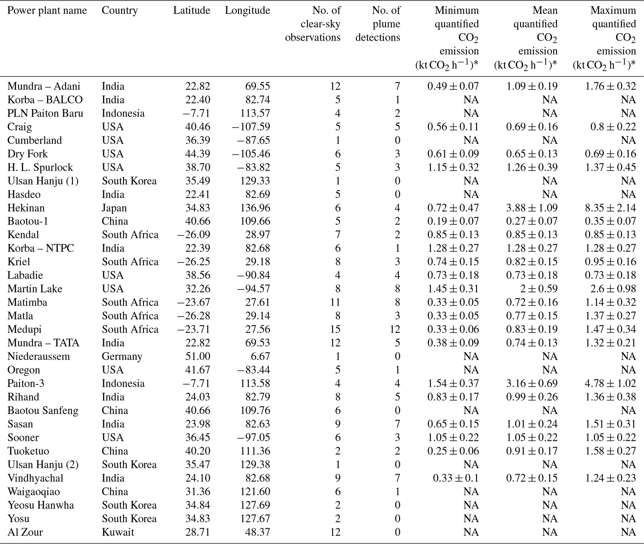
* “NA” indicates that no plumes were detected at this power plant or that the emission quantification algorithm (described in Sect. 2) failed to quantify an emission rate.
2.1 PRISMA observations and quantification
PRISMA is a tasked satellite instrument that is capable of collecting around 200 30 km × 30 km targets per day with a 20∘ off-nadir pointing capability. Authenticated users can program single observation requests through PRISMA's web portal (https://prisma.asi.it, last access: 16 November 2023), which currently allows for 13 concurrent requests at a time per user. We specified 2-week observing windows for each request and configured requests to collect if the scene-averaged solar zenith angle (SZA) was less than 70∘ and the forecast meteorology anticipated less than 20 % cloud cover. If the orbital configuration, weather, and SZA align and there are no other conflicting or higher-priority requests, PRISMA images a target.
For each acquired PRISMA image, we performed XCO2 retrievals on all pixels within a 2.5 km radius around the power plant. We retrieve XCO2 using the iterative maximum a posteriori – differential optical absorption spectroscopy (IMAP-DOAS) algorithm, as implemented in Cusworth et al. (2021). This approach estimates XCO2 by decomposing an observed radiance spectrum into high- and low-frequency features between 1900 and 2100 nm. For high-frequency features, we simulate atmospheric transmission of CO2, H2O, and N2O using a Beer–Lambert approximation. For low-frequency features (e.g., surface reflectance and aerosol scattering), we use an eighth-degree polynomial. Therefore, the forward model that drives IMAP-DOAS has the following form:
where Fh is simulated backscattered radiance at wavelength λ, I0 is incident solar intensity, Al is the air mass factor at vertical level l∈ [1,72], τn,l is the optical depth for each trace gas element, sn is the scaling factor applied to the optical depth, and ak is a polynomial coefficient (K=8). Optical depths are computed by querying meteorological information for pressure and temperature from the MERRA-2 (Modern-Era Retrospective analysis for Research and Applications, Version 2) reanalysis (Gelaro et al., 2017) and using that information to select proper High Resolution Transmission (HITRAN) absorption cross sections for each trace gas (Kochanov et al., 2016). To compare the model from Eq. (1) against PRISMA observed radiance (y), we compute Fh(x) between 1900 and 2100 nm at a 0.02 nm resolution, convolve the output using the PRISMA full width at half maximum, and sample at PRISMA wavelength positions. This results in vector F(x) that is comparable to y. The vector x, also called the state vector, includes scale factors for CO2, H2O, N2O, and polynomial coefficients: .
XCO2 is retrieved from PRISMA radiance using a Bayesian optimal estimation approach (Rodgers, 2000). Here, the optimized state vector solution, or posterior, is solved through Gauss–Newton iteration:
where SO= [εεT] is the observation error covariance matrix defined by the instrument signal-to-noise ratio (SNR), xA is the prior estimate of the state vector, and SA is the prior error covariance matrix. The matrix K, or Jacobian matrix, represents the first derivative of the F(x) with respect to the state vector:
The posterior error covariance matrix can be computed explicitly to quantify retrieval precision:
Across the scenes that we acquired with PRISMA, using this retrieval approach, we quantify an average 3.3 ppm precision for an XCO2 column. Absolute biases in PRISMA XCO2 retrievals are less important for CO2 plume detection and quantification: systematic retrieval biases are removed from a scene through the quantification and removal of a local background, as described below. To characterize bias in emission quantification, we compare emission rates derived from PRISMA to stack-level CEMS measurements (Sect. 3.2).
We quantified emissions for each PRISMA plume detection using the integrated mass enhancement (IME) approach (Cusworth et al., 2021). However, we updated the masking scheme for this analysis to produce more reliable masks for each CO2 plume. Figure 1 shows the plume-masking procedure for a plume detected at the Hekinan power plant, Japan, on 19 July 2021. First, we apply a background threshold to differentiate candidate plume pixels from the background (method to quantify background threshold described in Sect. 3.2). We then group enhanced XCO2 pixels into clusters of at least 20 connected pixels. These groups are then buffered with a one-pixel dilation filter to smooth edges and any gaps that exist in a group (Dougherty, 1992). Finally, each cluster is considered part of the plume if at least one of its pixels is within 500 m of an exhaust stack.
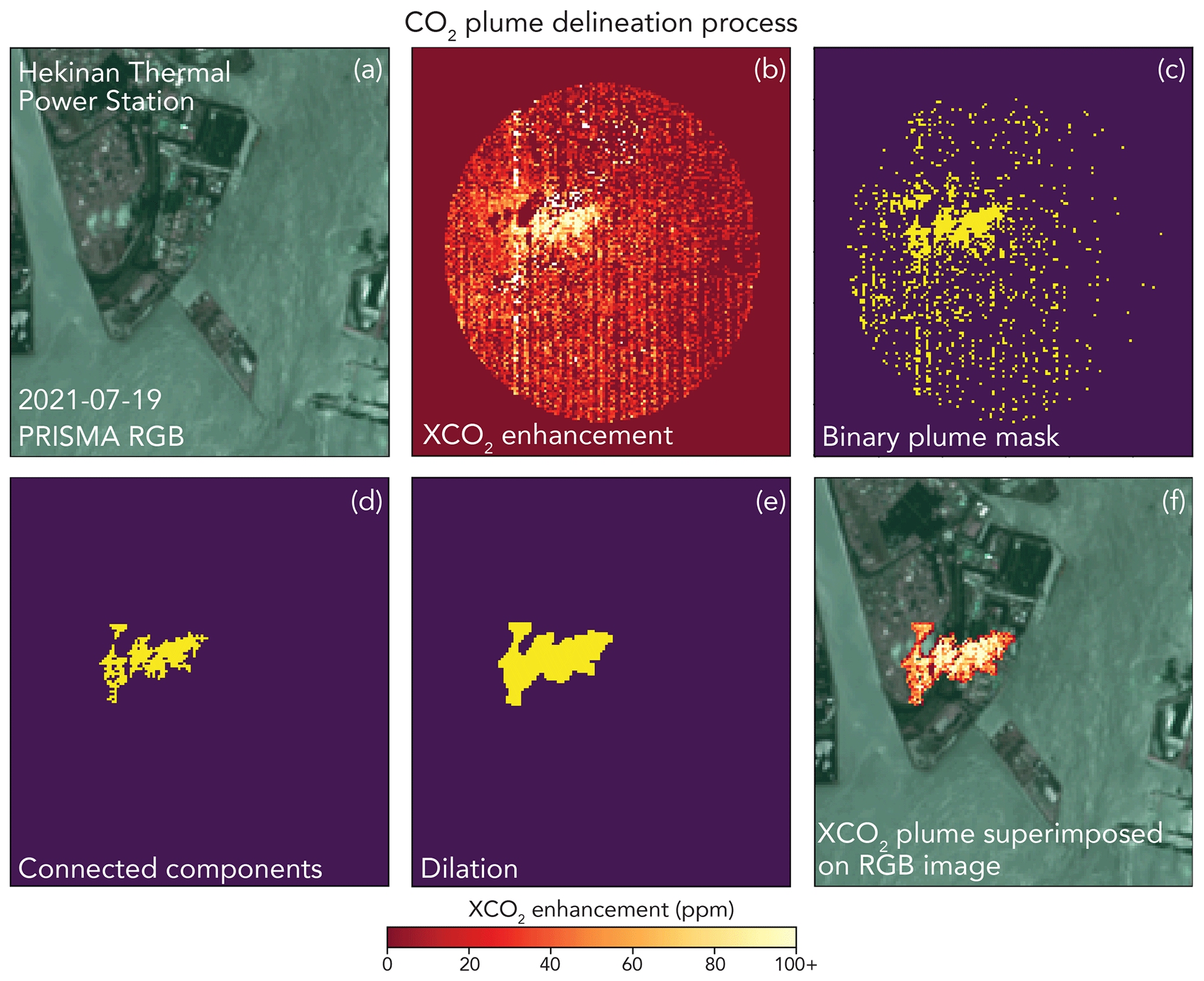
Figure 1Example of the plume delineation and masking process performed on XCO2 retrievals derived from PRISMA observations. Panel (a) shows the simultaneously observed RGB PRISMA imagery, panel (b) shows retrieved XCO2 above the background, panels (c)–(e) show the plume-masking procedure to isolate enhanced pixels and remove noise, and panel (f) shows the resulting CO2 plume superimposed on the RGB imagery.
IME is calculated for a plume using the following equation:
where ΔΩi is the XCO2 mass enhancement in pixel i relative to the background (kg m−2), Λi is the pixel area (900 m2), and N is the number of pixels in the plume. The CO2 emission rate Q is estimated from the IME using the following relationship:
where is the plume length and Ueff is the effective wind speed. The parameter L is an operational parameter that needs to be related to the extent of the plume. As a plume dissipates in all directions due to turbulent diffusion, an explicit scaling function (i.e., an effective wind speed Ueff) that relates L and 10 m wind speed (U10) to the true emission can be derived through large-eddy simulations (Varon et al., 2018):
where Ueff and U10 are in units of meters per second. We query the ERA5-Land reanalysis using the Open-Meteo application programming interface (https://open-meteo.com, last access: 16 November 2023), which provides hourly wind information globally at a 0.1∘ spatial resolution (Muñoz-Sabater et al., 2021). Uncertainty due to winds is calculated by generating an ensemble of U10 values assuming 50 % error (Cusworth et al., 2021). Uncertainty due to the CO2 background is calculated by generating many emission estimates and calculating a standard deviation using an ensemble of background thresholds. Background thresholds are set to vary with scene-averaged CO2 retrieval precision. Total emission uncertainty is estimated by adding in quadrature the contribution of wind and background uncertainties.
2.2 OCO-3 observations and quantification
OCO-3 is also a tasked mission: it can take SAM observations over any place of interest within the latitude range of the ISS orbit (about 52∘ S to 52∘ N). In addition to the SAM locations that we supplied to OCO-3 to overlap with PRISMA targets, there are many other power plant and fossil fuel combustion sources that make up its set of mission targets. However, unlike PRISMA, OCO-3 does not consider cloud forecasts, snow cover, or viewing geometry when planning SAM observations; thus, the majority of observations fail to produce useful maps of XCO2. Additionally, aerosol- and albedo-induced XCO2 artifacts are present in many SAM observations (Bell et al., 2023) and, thus, make the detection of plumes even more difficult.
For all cloud-free soundings, OCO-3 XCO2 concentrations are derived using the Atmospheric Carbon Observations from Space (ACOS; O'Dell et al., 2012, 2018; Crisp et al., 2012) v10 optimal estimation retrieval, which employs the Levenberg–Marquardt modification of the Gauss–Newton method. In this work, bias-corrected XCO2 from the OCO-3 Lite files is used, but the official data quality flag is not applied. This was done because the quality flag often removes XCO2 retrievals within the plume and makes emission estimation more difficult or impossible (Nassar et al., 2022). For SAM observations where we visually identified CO2 plumes (e.g., Fig. 2), emission rates are estimated using two approaches: (1) a Gaussian plume model and (2) the IME method. For the Gaussian plume model approach, we follow the algorithm outlined in Nassar et al. (2022):
Here, V represents the vertical columns within the plume (g m−2), Q is the CO2 emission rate (g s−1), y is the wind direction perpendicular to the plume (m), u is the wind speed at the height of the plume at its midline (m s−1) assuming plume rise of 250 m above the stack height, σy(x) is the standard deviation of the y direction, xo is a characteristic plume length (1000 m), and a is a stability parameter (Nassar et al., 2021). Following Nassar et al. (2022), wind speed and direction inputs are estimated by taking the average of the European Centre for Medium-Range Weather Forecasts Reanalysis Version 5 (ERA5) (Bell et al., 2021) and MERRA-2 reanalysis data. The wind direction is optimized by rotating the plume, typically between −30 and 30∘ away from the mean ERA5/MERRA-2 direction, and calculating the correlation coefficient (R) of the modeled and observed XCO2. The optimized wind direction is the direction that produces the largest R. The background is typically estimated by averaging OCO-3 footprints within a radius of 30 km, excluding the plume itself and a narrow 3 km buffer zone. However, if there are visible artifacts in the XCO2 background that are unrelated to the power plant plume, the background field is modified to avoid them – for example, by decreasing the radius of footprints used from 30 to 20 km. The uncertainty in the wind speed is calculated by taking the difference of the emission estimate using two different models (ERA5 and MERRA2). The background concentration uncertainty is calculated by estimating Q using three different background radii of 30, 40, and 50 km. Q is also calculated for a 30 km radius background but only using the left and right halves of the background, relative to the direction of the plume. The standard deviation of both of these methods is calculated and the larger of the two is the background uncertainty. The plume rise uncertainty is calculated by estimating Q using plume rise values of 100, 200, 250, 300, and 400 m and taking the standard deviation of those values. Total uncertainty in the emission rate Q using the Gaussian plume method is estimated by adding in quadrature the contribution of wind speed, background concentration, and plume rise uncertainties.
To obtain another estimate of emission rate, we also apply an IME quantification approach to the CO2 plumes, which (to our knowledge) is the first time that the IME method has been applied to OCO-3 SAM observations at coal power plants. We first interpolate the XCO2 retrievals in a SAM observation to a uniform 2 km × 2 km grid to account for occasional OCO-3 footprint overlap. Similar to Varon et al. (2018), 3 pixel × 3 pixel neighborhoods are sampled, and the distributions are compared to the background using a Student's t test. The default confidence level for the t test is 95 %, but this is often lowered to visually capture most of the plume. The plume is then smoothed using a 3 pixel × 3 pixel median filter and a Gaussian filter with a standard deviation of 0.5. The Ueff calculation is done using an equation approximately equal to Eq. (7) (). Other recent studies have used various methods (Lin et al., 2023; Brunner et al., 2023), but further research is needed to determine the most accurate way to estimate Ueff for an OCO-3-like instrument. The wind direction is the optimized direction determined by the Gaussian plume model. The background XCO2 estimate is taken from the Gaussian plume model methodology and the plume is typically required to be within 50 km downwind and 8 km crosswind of the source, although these parameters are modified if the plume curves outside of the 8 km crosswind threshold or there are XCO2 artifacts that should be avoided.
The uncertainty in the IME method is estimated similarly to the Gaussian plume model method. The uncertainty in wind speed is calculated by taking the standard deviation of the emission estimates using wind speed from two different models (ERA5 and MERRA2). The background concentration uncertainty is calculated by estimating Q using the different backgrounds calculated in the Gaussian plume model method: a 20 km radius, 30 km radius, 40 km radius, left half, full circle, and right half. The standard deviation of the three radii estimates and of the left half, full circle, and right half estimates are calculated, and the larger of the two is the background uncertainty. The uncertainty in the Student's t test confidence level is also estimated. The confidence level and −10 % and +10 % of the confidence level are used to find Q. For example, if the confidence level needed to visually capture the XCO2 plume is 85 %, Q is calculated for 75 %, 85 %, and 95 % and the standard deviation of those three values represents the confidence level uncertainty. Total uncertainty in the emission rate Q using the IME method is estimated by adding in quadrature the contribution of the wind speed, background concentration, and Student's t test confidence level uncertainties.
Figure 2 shows the IME methodology successfully identifying an XCO2 plume from an OCO-3 SAM observation taken over the Colstrip power plant.
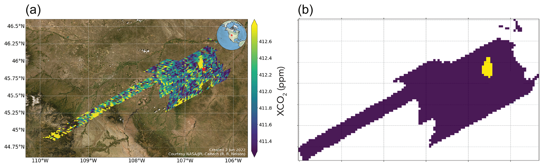
Figure 2The IME plume identification approach applied to an example OCO-3 SAM observation at the Colstrip Power Plant on 18 August 2021. Panel (a) shows the OCO-3 SAM bias-corrected XCO2. In panel (b), the yellow pixels indicate the final plume mask.
3.1 Global yields from 2 years of observations
Figure 3a shows a global map of the power plants that we targeted with PRISMA, with the marker for each power plant's location (latitude and longitude) scaled to represent the number of successful acquisitions between 2021 and 2022. In total, we acquired 181 PRISMA images, which correspond to 314 unique power plant observation scenes. Of these scenes, 210 were of sufficient quality to attempt CO2 retrieval and plume detection, with quality mostly determined by visual inspection for clouds and haze. Of these 210 scenes, 104 were determined to have CO2 plumes (Fig. 3b). Scenes were marked as containing CO2 plumes through inspection of XCO2 and visible imagery: if a large cluster of pixels with elevated XCO2 above the background were also in the vicinity of a power plant exhaust stack, an analyst would mark the scene as containing a CO2 plume. Routine tasking observations with PRISMA resulted in an average of 6 acquisitions for each power plant (maximum 15), roughly 1 image acquired per quarter. Of these acquisitions, plumes were detected on average 4 times per facility (maximum 12).
For OCO-3, 1363 power plant SAM observations were taken during the period from September 2019 to December 2022. Of these, 139 XCO2 plumes emanating from power plants were visually identified. However, only 14 were for power plants that were also observed by PRISMA and have CEMS validation (9 Colstrip cases, 2 Martin Lake cases, and 3 Craig cases). The acquisition rates are low relative to PRISMA because OCO-3 does not account for scene favorability when planning its SAM observations. For example, OCO-3 took 66 Colstrip SAM observations from 2019 to 2022 but only yielded 9 high-quality XCO2 plume cases.
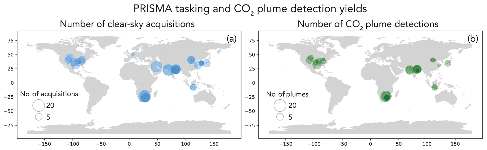
Figure 3Data yields from PRISMA continually between 2021 and 2022. Panel (a) shows the number of clear-sky acquisitions for each power plant. Panel (b) shows the number of plumes detected by an analyst for each of the observed power plants.
The low observed average detection rate of CO2 plumes is a result of three primary factors: (1) the observing conditions at each facility, including solar zenith angle (SZA) and surface reflectance; (2) the local meteorology; and (3) the operational status at each power plant at the time of acquisition. To test how well these factors predict the presence of a plume for PRISMA, we fit a logistic regression classification function with a sparse (L1) penalty to our dataset (Fan et al., 2008). This algorithm fits a logit function to the plume detection outcome of each scenes (i.e., detected plume is TRUE, whereas no detected plume is FALSE) using a set of predictor variables that are likely candidates to explain prediction results. In this setup, the statistical model is fit using the following predictor variables: SZA, U10, average single-sounding retrieval precision across the scene, annual bottom-up emission estimate for the power plant using GEM, and average observed radiance between 1900 and 2100 nm within the scene normalized by the cosine of the SZA. This last factor is a simple proxy for surface reflectance, although it does not take into account other factors that influence radiance observations (e.g., water vapor, aerosols, and other atmospheric constituents). We split the data so that 50 % was used to train the model and 50 % was reserved as a test set. The predictor variables were all standardized by their mean and standard deviation before the model was fit. The results of classification can be summarized using two statistics: precision (ratio of true positives to sum of true positives and false positives) and recall (ratio of true positives to sum of true positives and false negatives). The results of fitting a logistic regression model to the data show minor prediction performance, with precision =0.60 and recall =0.69 for positive plume detection. The regression coefficients are shown in Fig. 4a. The coefficient with the highest weight is normalized radiance. Figure 4b shows the SZA against normalized radiance, with red dots indicating no plume detection and blue dots representing positive plume detection. Although no clear separation exists, there is a cluster of no plume detection at a high SZA and low normalized radiance. This is a consistent and expected relationship, as SZA and surface reflectance are principal drivers of the quantity of light that is observed by the satellite, and therefore the SNR of the observation.
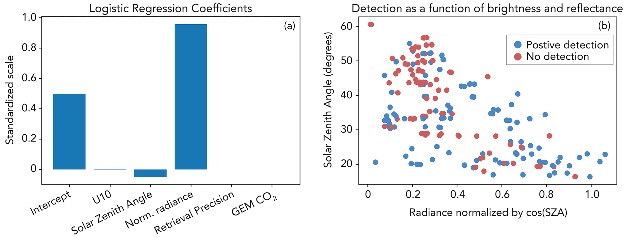
Figure 4CO2 plume prediction using various atmospheric, retrieval, and bottom-up information. Panel (a) shows the results of fitting a logistic regression classification model to the set of PRISMA acquisitions where an analyst identified the presence or lack of a plume. Panel (b) shows the top two explanatory variables (SZA and normalized radiance) along with plume classification.
The logistic regression model performed better on the test dataset than predictions made at random, although the prediction performance was still low. Missing from the model is sub-annually resolved information regarding operating status. For most of the power plants outside the USA, we do not have information on daily operations. In many cases of non-detects, we could simply be observing a power plant temporarily not in operation. Another possibility is that some power plants were operating at reduced capacity at the time of acquisition, meaning that CO2 emission rates were lower than those predicted by annual emission factors or activity data. If the true CO2 emission rate was below the minimum detection limit (MDL) of the PRISMA satellite, it would show as a non-detect. However, even if the emission were near or slightly above the PRISMA MDL, the probability of detection would still be low, as slight variations in atmospheric properties (as seen in Fig. 4) would then influence the ability to detection a CO2 plume.
3.2 Validation of PRISMA and OCO-3 emission rates against CEMS
For each power plant where a CO2 plume was identified, we quantify emissions using the IME approach described by Eqs. (5)–(7). In order to estimate the XCO2 mass enhancement (ΔΩ in Eq. 1), a local background must be quantified and subtracted from total XCO2 retrievals across the scene. To do this, we apply a concentration threshold β to initiate the plume-masking and segmentation process (described in Sect. 2). Once we have a plume mask, we apply another concentration threshold γ to the remaining XCO2 pixels that exist outside of the plume. This value γ represents the XCO2 background that we use to calculate the XCO2 enhancement that is used in the IME formulation of Eq. (1). Thresholds β and γ largely influence the magnitude of the emission rate and are not known a priori. For global generalizability, we wish to estimate β and γ such that they do not vary across power plants, seasons, regions, etc. Therefore, we parameterize β and γ as percentiles under the assumption that the local contrast between enhanced CO2 plume pixels and the background should be similar across PRISMA scenes.
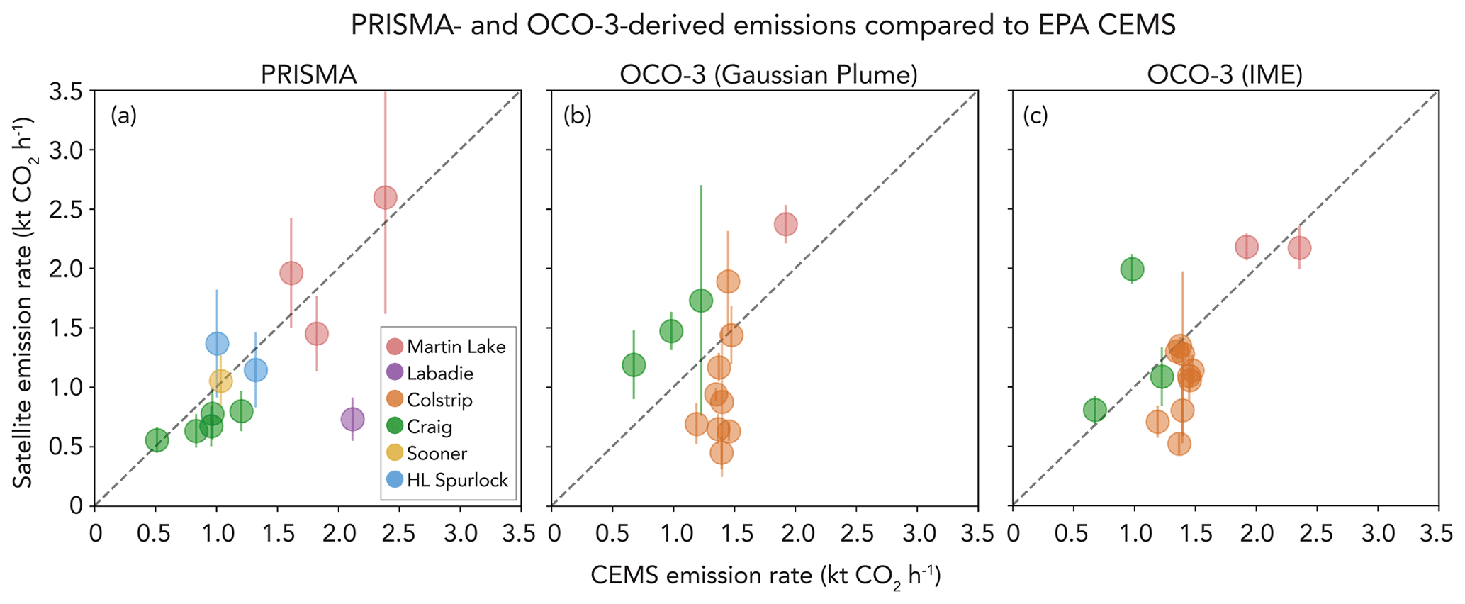
Figure 5Comparison of emission rates in the USA between satellite-derived estimates and CEMS information. Panel (a) shows a comparison between PRISMA-derived emission rates and CEMS (R2=0.43), panel (b) shows a comparison between OCO-3 and CEMS using the Gaussian plume model (R2=0.51), and panel (c) shows a comparison between OCO-3 and CEMS using IME (R2=0.32).
To estimate values for β and γ, we compare EPA CEMS data for power plants in the USA with estimated emission rates from PRISMA. In total, we have 12 scenes in the USA with CEMS information that pertain to 5 power plants. We then optimize β and γ such that the output of an ordinary least squares regression produces a slope near unity. Figure 5a shows the results of this optimization which produces an optimal β percentile of 94 % and a γ percentile of 62 %.The results also show a decent correlation between CEMS data and PRISMA-derived emission rates (R2=0.43). A single outlier at the Labadie power plant (imaged 10 July 2022) shows the largest discrepancy from CEMS data (69 %), but the remaining plumes show an average 27 % relative difference from CEMS data. If we remove the one data point at Labadie, the R2 improves to 0.75. Although a limited sample size, between PRISMA and OCO-3, these scenes represent variability in solar geometries (20–40∘ SZA), surface reflectance (0.09–0.90 normalized radiance), and reported emission rates (0.51–2.39 kt CO2 h−1). Therefore, we use these optimal parameters and apply them to our global dataset of PRISMA detections. These emission rates are reported in Table 1. There are some instances in which performing IME emission calculations using these thresholds and plume-masking technique do not result in emission rates (e.g., the plume-masking procedure produces a mask with no pixels). In these cases, we report a detection but not an emission quantification.
Figure 5b and c show the comparison between OCO-3 and CEMS at some power plants that overlap with PRISMA observations (14 scenes total). OCO-3 Gaussian plume model emission rates (Fig. 5b) have an improved correlation compared with PRISMA (R2=0.51), although with greater bias (average 47 % relative difference from CEMS). The OCO-3 IME estimates (Fig. 5c) have a worse R2 (0.32) but a better RMSE (0.45 kt CO2 h−1) compared with the Gaussian plume model estimates (0.84 kt CO2 h−1), with 9 of the 14 cases being within 30 % of the reported CEMS emission and an average relative difference of 30 % for all 14 cases. Additionally, the least squares fit for IME is closer to the one-to-one line than for the Gaussian plume model.
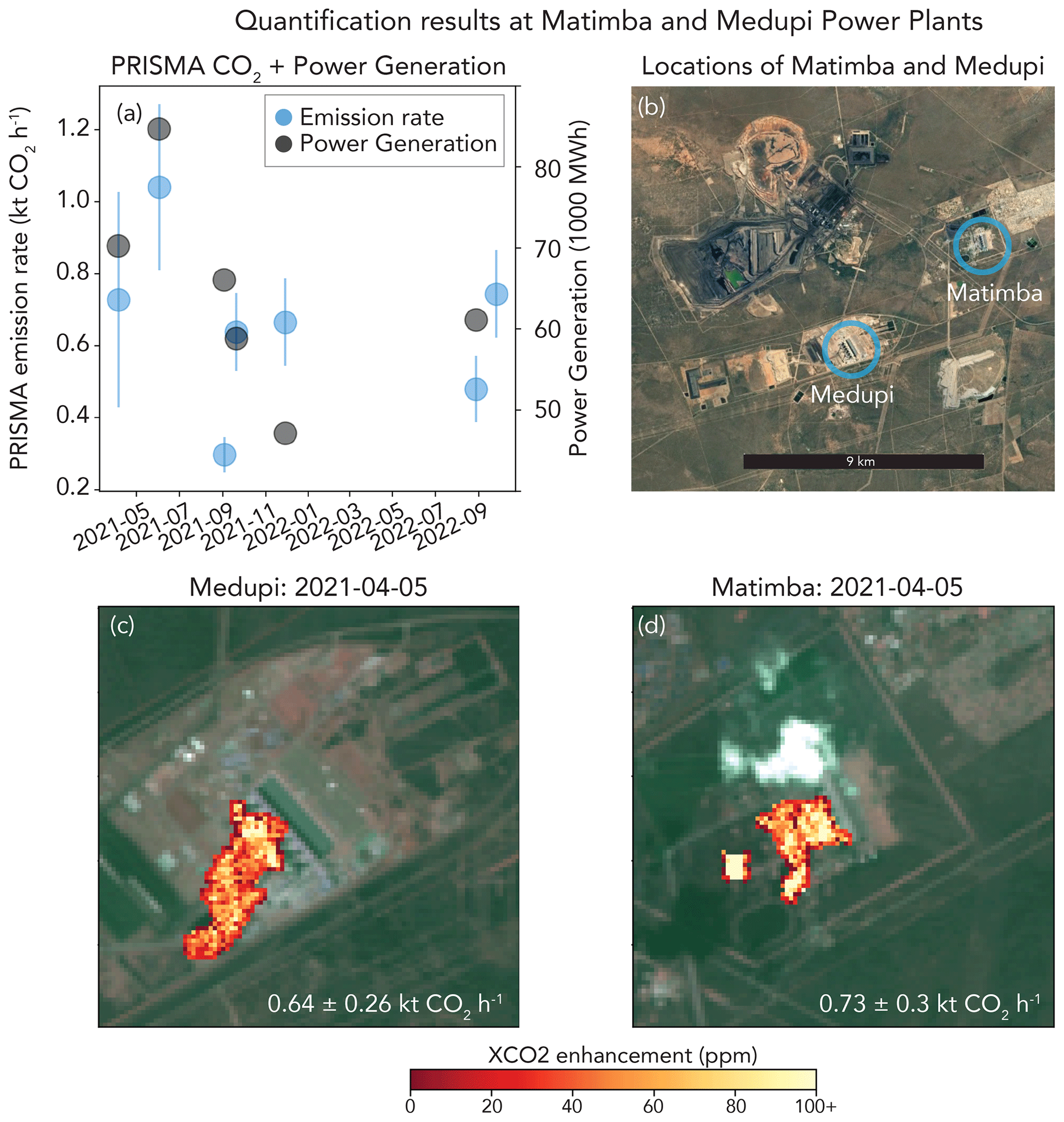
Figure 6Emission rates and reported power generation at the Matimba and Medupi power plants in South Africa. Panel (a) shows the CO2 emission rates derived from PRISMA and the reported daily power generation for the day of PRISMA overpass, panel (b) shows the locations of the Medupi and Matimba power plants (base imagery provided by Google Earth; © Google Earth 2023), and panels (c) and (d) show plume imagery and emission rates for a PRISMA overpass on 5 April 2021.
Unique sources of error for OCO-3 emission estimates include geolocation errors in the XCO2 product. These errors are typically less than 1 km but can be up to 2 km (Taylor et al., 2023). Errors of this magnitude, about the size of an OCO-3 footprint (∼ 2 km × 2 km), may mean that an entire footprint is not included when estimating emissions using the Gaussian plume method, which assumes that the plume only extends downwind of the known source location. The Gaussian plume model is also susceptible to wind direction errors and requires the plume to be Gaussian in shape, the latter of which is often not true. IME, while not suffering from wind-direction- or geolocation-induced errors, assumes that the entire plume is captured in a given SAM observation, which is sometimes not true and results in an underestimation of emissions. IME is also sensitive to errors in Ueff parameterization.
3.3 Comparison and fusion of PRISMA and OCO
Outside the USA, PRISMA observed the Matimba power station in South Africa 11 times and quantified emission rates 7 times. Emissions from Matimba have previously been quantified and validated using OCO-2 (Hakkarainen et al., 2021). This station does not report hourly emission rates, but it does report daily power generation (Eskom, 2023). Although not a direct comparison, we can use this information to check if the emission quantification approach that we describe above captures some variability in activity at this power plant. Figure 6a shows the emission rates that we quantified compared against reported power generation. We see rough agreement in variability: the high power generation reported between April and July 2021 (70 000–85 000 MW h) drops for subsequent dates (47 000–66 000 MW h) between September 2021 and September 2022, a drop which is also seen in the PRISMA-derived CO2 emission rate. Across all observations, we estimate an emission rate range of 0.30–1.04 kt CO2 h−1 (average of 0.66 kt CO2 h−1). This average emission rate is substantially lower than the average 2.50 kt CO2 h−1 emission rate estimated from OCO-2 and TROPOMI between 2018 and 2020, but it is within the range of emissions estimates directly quantified with OCO-2 (0.30–7.20 kt CO2 h−1; Hakkarainen et al., 2021). However, this discrepancy could be result of (1) changes in activity or variability or (2) the existence of other nearby emission sources. For changes in activity, during August 2020, the Matimba reported a large range of power generation (65 000–94 000 MW h), and emission estimates derived directly from OCO-2 were also highly variable (0.88–4.33 kt CO2 h−1). Given that maximum power generation at the time of a PRISMA observation was 85 000 MW h, some of the discrepancy in maximum CO2 quantification between PRISMA and OCO-2 could be due to activity.
Near (7 km) the Matimba Power Station is the Medupi Power Station (Fig. 6b). Figure 6c shows the Medupi CO2 plume observed during the same PRISMA overpass on 5 April 2021. The PRISMA-derived emission rate is 0.64±0.26 kt CO2 h−1 for Medupi and 0.73±0.30 kt CO2 h−1 for Matimba. Given the proximity of the two power plants, the higher derived emission rate reported for Matimba from previous studies could actually be a result of a net emission from these two facilities. The OCO-2 flight track is located tens of kilometers downwind of Matimba and Medupi, making a clear delineation between potentially co-emitted distinct emission plumes almost impossible. If we sum emission rates from both Medupi and Matimba, we quantify a range of 0.89–1.73 kt CO2 h−1 (average of 1.30±0.28 kt CO2 h−1), which, although still lower, is closer to the average emissions quantified by OCO-2.
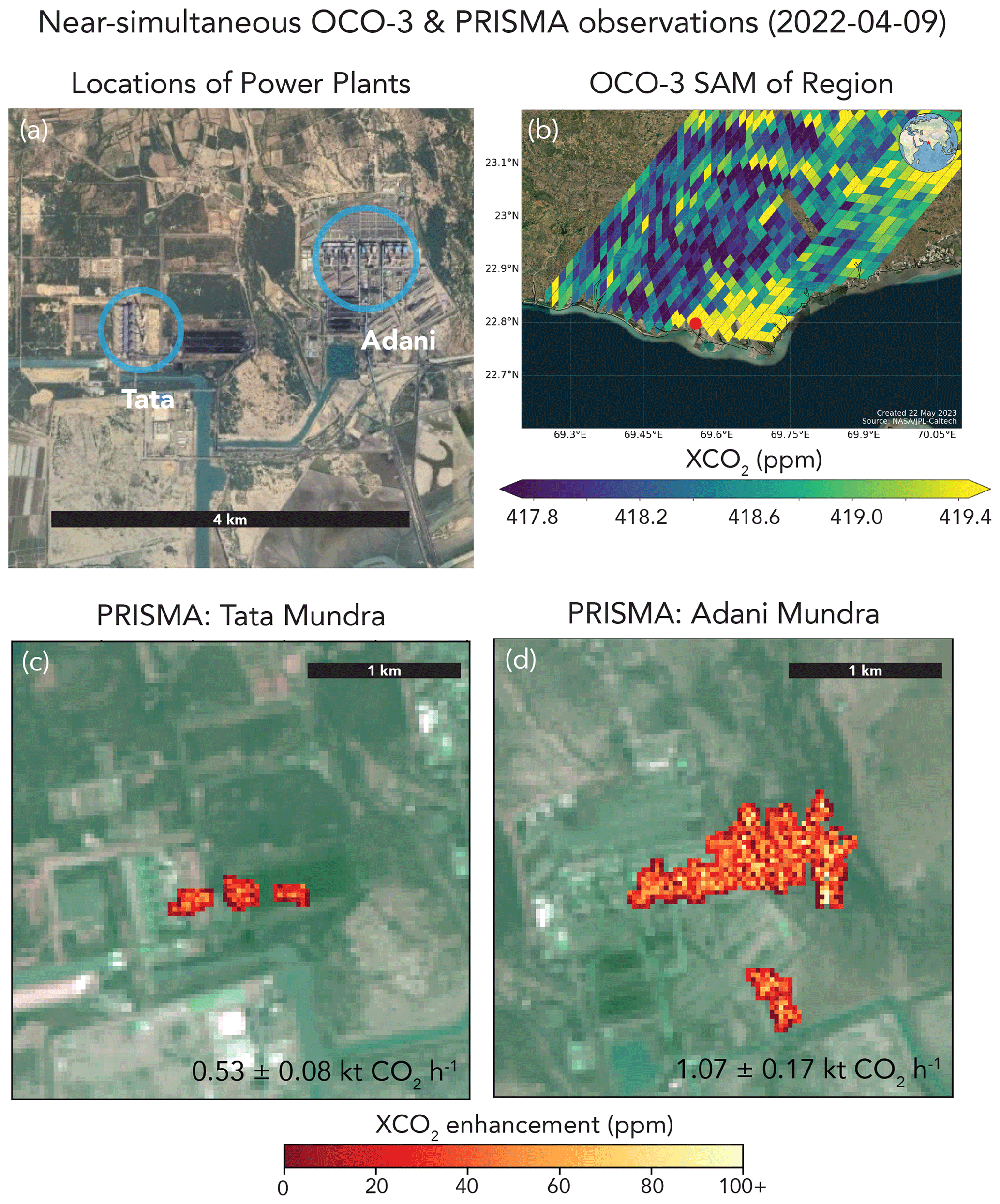
Figure 7Near-simultaneous observation of two power plants in Mundra, India, on 9 April 2022. Panel (a) shows the locations of two power plants, Mundra –TATA and Mundra – Adani, spaced less than 3 km apart (base imagery provided by Google Earth; © Google Earth 2023); panel (b) presents the OCO-3 SAM observation, with a red dot showing the location of the power plants; and panels (c) and (d) show the PRISMA acquisition (less than 2 h after OCO-3) over the two power plants with the associated emission rates.
The ability to differentiate the contribution of unique point sources to a regional total is an application made possible by joint observations from imaging spectrometers and atmospheric sounders. Figure 7 shows observations that were made at the Mundra TATA Ultra Mega Power Plant and the Mundra Adani Thermal Power Project: two power plants less than 3 km apart. Both OCO-3 and PRISMA imaged the power plants on 9 April 2022. Figure 7b shows the OCO-3 SAM observation (taken at 04:41 UTC): large CO2 enhancements appear along the coastline, likely associated with emission from these power plants. PRISMA imaged the power plants less than 2 h later (at 06:02 UTC) and detected CO2 plumes at each facility (Fig. 7b, c). The OCO-3-derived emission rate using Gaussian plume approaches is 5.5±0.7 kt CO2 h−1, but the emission rate derived using the IME approach is much lower (3.0 kt CO2 h−1). For this case, the IME approach may be more appropriate, as the shape of the OCO-3 plume (Fig. 7b) is more diffuse in nature and does not visibly resemble a Gaussian structure. The PRISMA emission rate is 1.07±0.17 kt CO2 h−1 for the Adani plant and 0.53±0.08 kt CO2 h−1 for the Mundra TATA plant. We can use this information to estimate that 67 % of the net CO2 emission was from Adani and the remaining 33 % was from the TATA plant. The combined emission rate (1.60±0.25 kt CO2 h−1) is lower than the OCO-3 IME emission rate. Like the Matimba power plant, some of this discrepancy may partially be explained by bias or uncertainty in retrievals, background, and wind information. Also, lower estimates of CO2 emissions from PRISMA are consistent with the fact that PRISMA is only sensitive to emissions at two exhaust stacks, while the OCO-3 observation includes all CO2 sources in the industrial area around Mundra. Continued validation of retrieved emission rates against ground standards (e.g., CEMS) will help better quantify bias and uncertainty. However, even with lingering uncertainty, the near-simultaneous observations of OCO-3 and PRISMA can help us disentangle the relative contributions from each power plant.
We observed a global set of power plants for 2 years between 2021 and 2022 with both PRISMA and OCO-3 to test the ability of these satellite platforms to carry out routine operational monitoring of CO2 emissions. When PRISMA observations were of sufficient quality to perform XCO2 retrievals, we detected CO2 plumes nearly half of the time. We fit a logistic regression classification using plume detections and find that there is some relationship between the SZA and surface reflectance that partially explains plume prediction; this is consistent with the fact that these factors are major drivers of the SNR. The remaining non-plume detections may be due to the operational status of a power plant at the time of observation. We compared emission rates from both PRISMA and OCO-3 to power plants in the USA, where we have access to hourly in situ CEMS emission information. We find a significant correlation between satellite and in situ estimates, although some significant biases may exist for some of the observations for both PRISMA and OCO-3. Also, the quantity of CEMS observations was limited (∼10 for each instrument), so robust calibration is not yet possible. Still, early results show that under the right conditions, satellites can provide reliable estimates of CO2 emissions at discrete point source locations. This is consistent with the close agreement between airborne imaging spectrometer emissions and CEMS information (Cusworth et al., 2021).
Fusion of information from atmospheric sounders, like OCO-3, and imaging spectrometers, like PRISMA, is valuable for cross-validation and source attribution. We see this particularly for our examples at the Matimba and Medupi power plants in South Africa and the TATA and Adani power plants in Mundra, India. In these cases, and particularly at Mundra where near-simultaneous PRISMA and OCO-3 observations were taken, OCO-2 and OCO-3 provide a local but coarse-resolution emission constraint for a complex of facilities that emit large CO2 quantities. PRISMA, with its 30 m pixel resolution, can then help refine the relative contributions of single emitters against the net emission flux. More work is needed to refine cross-validation between instruments, but initial observation shows one avenue for data from multiple observing systems to be combined and analyzed.
Even when combining information from both satellites, there are still too few samples to constrain facility emissions within low uncertainties. Cusworth et al. (2021), using arguments from Hill and Nassar (2019), suggested that nearly 30 unbiased observations from a PRISMA-class instrument are needed per year at each power plant to reduce annual uncertainties below 14 % (i.e., reduce emission uncertainty from Non-Annex I countries to below 1 Gt CO2 yr−1). No power plant in this study met this minimum sampling requirement. However, there will be a significant increase in data volumes and observation performance of satellite remote-sensing capabilities for CO2, from both recently launched and planned imaging spectrometers, including the Earth surface Mineral dust source InvesTigation instrument (EMIT – launched 2022; Thorpe et al., 2023), the Environmental Mapping and Analysis Program instrument (EnMAP – launched 2022; Guanter et al., 2015), and the Carbon Mapper/Tanager 1–2 (planned launch in 2024; Duren et al., 2021), and atmospheric sounders, including the Copernicus Carbon Dioxide Monitoring mission instrument (CO2M; Sierk et al., 2019). Improved observation of global power plants and emission quantification with robust error characterization will be vital to reduce global uncertainty in anthropogenic emissions from fossil fuel combustion sources.
The OCO-3 XCO2 and other retrieval products are publicly available from the NASA Goddard Earth Science (GES) Data and Information Services Center (DISC). The full suite of retrieval products in the standard per-orbit format can be obtained from https://doi.org/10.5067/D9S8ZOCHCADE (OCO Science Team, 2021) and the lightweight per-day format data (Lite files), which include the bias-corrected estimates of XCO2, can be obtained from https://doi.org/10.5067/970BCC4DHH24 (OCO-2/OCO-3 Science Team, 2022). PRISMA data, including radiance for each scene and XCO2 retrievals, are available from a Zenodo data repository (https://doi.org/10.5281/zenodo.8083596, Cusworth, 2023).
DHC designed the study. DHC, AKA, and RJ requested and acquired PRISMA data. DHC performed PRISMA emission quantification and validation. RRN performed OCO-3 quantification and validation. RN and JPM helped implement OCO-3 quantification algorithms. All authors provided feedback on the results and the manuscript.
The contact author has declared that none of the authors has any competing interests.
Publisher’s note: Copernicus Publications remains neutral with regard to jurisdictional claims made in the text, published maps, institutional affiliations, or any other geographical representation in this paper. While Copernicus Publications makes every effort to include appropriate place names, the final responsibility lies with the authors.
This work was supported by the Orbiting Carbon Observatory Science Team. We thank the Italian Space Agency for the PRISMA satellite targets. Portions of this work were undertaken at the Jet Propulsion Laboratory, California Institute of Technology, under contract with NASA.
This research has been supported by the National Aeronautics and Space Administration.
This paper was edited by Qiang Zhang and reviewed by two anonymous referees.
Beirle, S., Borger, C., Dörner, S., Eskes, H., Kumar, V., de Laat, A., and Wagner, T.: Catalog of NOx emissions from point sources as derived from the divergence of the NO2 flux for TROPOMI, Earth Syst. Sci. Data, 13, 2995–3012, https://doi.org/10.5194/essd-13-2995-2021, 2021.
Bell, B., Hersbach, H., Berrisford, P., Dahlgren, P., Horányi, A., Sabater, M., Nicolas, J., Radu, R., Schepers, D., Soci, C., Villaume, S., Bidlot, J., Haimberger, L., Woollen, J., Buontempo, C., and Thépaut, J.: ERA5 hourly data on pressure levels from 1950 to 1978 (preliminary version), Copernic. Clim. Change Serv. (C3S) Clim. Data Store (CDS), https://cds.climate.copernicus.eu/cdsapp#!/dataset/reanalysis-era5-pressure-levels-preliminary-back-extension?tab=overview (last access: 16 November 2023), 2021.
Bell, E., O'Dell, C. W., Taylor, T. E., Merrelli, A., Nelson, R. R., Kiel, M., Eldering, A., Rosenberg, R., and Fisher, B.: Exploring bias in the OCO-3 snapshot area mapping mode via geometry, surface, and aerosol effects, Atmos. Meas. Tech., 16, 109–133, https://doi.org/10.5194/amt-16-109-2023, 2023.
Brunner, D., Kuhlmann, G., Henne, S., Koene, E., Kern, B., Wolff, S., Voigt, C., Jöckel, P., Kiemle, C., Roiger, A., Fiehn, A., Krautwurst, S., Gerilowski, K., Bovensmann, H., Borchardt, J., Galkowski, M., Gerbig, C., Marshall, J., Klonecki, A., Prunet, P., Hanfland, R., Pattantyús-Ábrahám, M., Wyszogrodzki, A., and Fix, A.: Evaluation of simulated CO2 power plant plumes from six high-resolution atmospheric transport models, Atmos. Chem. Phys., 23, 2699–2728, https://doi.org/10.5194/acp-23-2699-2023, 2023.
Crippa, M., Guizzardi, D., Banja, M., Solazzo, E., Muntean, M., Schaaf, E., Pagani, F., Monforti-Ferrario, F., Olivier, J., Quadrelli, R., Risquez Martin, A., Taghavi-Moharamli, P., Grassi, G., Rossi, S., Jacome Felix Oom, D., Branco, A., San-Miguel-Ayanz, J., and Vignati, E.: CO2 emissions of all world countries – 2022 Report, EUR 31182 EN, Publications Office of the European Union, Luxembourg, https://doi.org/10.2760/730164, JRC130363, 2022.
Crisp, D., Fisher, B. M., O'Dell, C., Frankenberg, C., Basilio, R., Bösch, H., Brown, L. R., Castano, R., Connor, B., Deutscher, N. M., Eldering, A., Griffith, D., Gunson, M., Kuze, A., Mandrake, L., McDuffie, J., Messerschmidt, J., Miller, C. E., Morino, I., Natraj, V., Notholt, J., O'Brien, D. M., Oyafuso, F., Polonsky, I., Robinson, J., Salawitch, R., Sherlock, V., Smyth, M., Suto, H., Taylor, T. E., Thompson, D. R., Wennberg, P. O., Wunch, D., and Yung, Y. L.: The ACOS CO2 retrieval algorithm – Part II: Global X data characterization, Atmos. Meas. Tech., 5, 687–707, https://doi.org/10.5194/amt-5-687-2012, 2012.
Crisp, D., Pollock, H. R., Rosenberg, R., Chapsky, L., Lee, R. A. M., Oyafuso, F. A., Frankenberg, C., O'Dell, C. W., Bruegge, C. J., Doran, G. B., Eldering, A., Fisher, B. M., Fu, D., Gunson, M. R., Mandrake, L., Osterman, G. B., Schwandner, F. M., Sun, K., Taylor, T. E., Wennberg, P. O., and Wunch, D.: The on-orbit performance of the Orbiting Carbon Observatory-2 (OCO-2) instrument and its radiometrically calibrated products, Atmos. Meas. Tech., 10, 59–81, https://doi.org/10.5194/amt-10-59-2017, 2017.
Cusworth, D.: CO2 retrievals at global power plants using PRISMA satellite data, Zenodo [data set], https://doi.org/10.5281/zenodo.8083596, 2023.
Cusworth, D. H., Duren, R. M., Thorpe, A. K., Eastwood, M. L., Green, R. O., Dennison, P. E., Frankenberg, C., Heckler, J. W., Asner, G. P., and Miller, C. E.: Quantifying global power plant carbon dioxide emissions with imaging spectroscopy, AGU Adv., 2, e2020AV000350, https://doi.org/10.1029/2020AV000350, 2021.
Dougherty, E. R.: An introduction to morphological image processing, in: SPIE Optical Engineering Press, ISBN-10:081940845X, 1992.
Duren, R., Cusworth, D., Ayasse, A., Herner, J., Thorpe, A., Falk, M., Heckler, J., Guido, J., Giuliano, P., Chapman, J., and Green, R.: December, Carbon Mapper: on-orbit performance predictions and airborne prototyping, in: AGU Fall Meeting Abstracts, December 2021, New Orleans, Louisiana, USA, A53F-05, https://ui.adsabs.harvard.edu/abs/2021AGUFM.A53F..05D (last access: 16 November 2023), 2021.
Eldering, A., Taylor, T. E., O'Dell, C. W., and Pavlick, R.: The OCO-3 mission: measurement objectives and expected performance based on 1 year of simulated data, Atmos. Meas. Tech., 12, 2341–2370, https://doi.org/10.5194/amt-12-2341-2019, 2019.
Eskom: Atmospheric emissions license reports, https://www.eskom.co.za/dataportal/emissions/ael/matimba-c2/ (last access: 16 November 2023), 2023.
Fan, R. E., Chang, K. W., Hsieh, C. J., Wang, X. R., and Lin, C. J.: LIBLINEAR: A library for large linear classification, J. Mach. Learn. Res., 9, 1871–1874, 2008.
Gelaro, R., McCarty, W., Suárez, M. J., Todling, R., Molod, A., Takacs, L., Randles, C. A., Darmenov, A., Bosilovich, M. G., Reichle, R., and Wargan, K.: The modern-era retrospective analysis for research and applications, version 2 (MERRA-2), J. Climate, 30, 5419–5454, https://doi.org/10.1175/JCLI-D-16-0758.1, 2017.
GEM: Global Energy Monitor's Global Coal Plant Tracker, https://globalenergymonitor.org/projects/global-coal-plant-tracker/tracker/, last access: 24 May 2023.
Guan, D., Liu, Z., Geng, Y., Lindner, S., and Hubacek, K.: The gigatonne gap in China's carbon dioxide inventories, Nat. Clim. Change, 2, 672–675, https://doi.org/10.1038/nclimate1560, 2012.
Guanter, L., Kaufmann, H., Segl, K., Foerster, S., Rogass, C., Chabrillat, S., Kuester, T., Hollstein, A., Rossner, G., Chlebek, C., and Straif, C.: The EnMAP spaceborne imaging spectroscopy mission for earth observation, Remote Sens., 7, 8830–8857, https://doi.org/10.3390/rs70708830, 2015.
Guo, W., Shi, Y., Liu, Y., and Su, M.: CO2 emissions retrieval from coal-fired power plants based on OCO-2/3 satellite observations and a Gaussian plume model, J. Clean. Prod., 397, 136525, https://doi.org/10.1016/j.jclepro.2023.136525, 2023.
Hakkarainen, J., Szeląg, M. E., Ialongo, I., Retscher, C., Oda, T., and Crisp, D.: Analyzing nitrogen oxides to carbon dioxide emission ratios from space: A case study of Matimba Power Station in South Africa, Atmos. Environ., 10, 100110, https://doi.org/10.1016/j.aeaoa.2021.100110, 2021.
Hill, T. and Nassar, R.: Pixel size and revisit rate requirements for monitoring power plant CO2 emissions from space, Remote Sens., 11, 1608, https://doi.org/10.3390/rs11131608, 2019.
Hong, C., Zhang, Q., He, K., Guan, D., Li, M., Liu, F., and Zheng, B.: Variations of China's emission estimates: response to uncertainties in energy statistics, Atmos. Chem. Phys., 17, 1227–1239, https://doi.org/10.5194/acp-17-1227-2017, 2017.
IPCC: Climate Change 2021: The Physical Science Basis, Contribution of Working Group I to the Sixth Assessment Report of the Intergovernmental Panel on Climate Change, edited by: Masson-Delmotte, V., Zhai, P., Pirani, A., Connors, S. L., Péan, C., Berger, S., Caud, N., Chen, Y., Goldfarb, L., Gomis, M. I., Huang, M., Leitzell, K., Lonnoy, E., Matthews, J. B. R., Maycock, T. K., Waterfield, T., Yelekçi, O., Yu, R., and Zhou, B., Cambridge University Press, Cambridge, United Kingdom and New York, NY, USA, in press, https://doi.org/10.1017/9781009157896, 2021.
Muñoz-Sabater, J., Dutra, E., Agustí-Panareda, A., Albergel, C., Arduini, G., Balsamo, G., Boussetta, S., Choulga, M., Harrigan, S., Hersbach, H., Martens, B., Miralles, D. G., Piles, M., Rodríguez-Fernández, N. J., Zsoter, E., Buontempo, C., and Thépaut, J.-N.: ERA5-Land: a state-of-the-art global reanalysis dataset for land applications, Earth Syst. Sci. Data, 13, 4349–4383, https://doi.org/10.5194/essd-13-4349-2021, 2021.
Kochanov, R. V., Gordon, I. E., Rothman, L. S., Wcisło, P., Hill, C., and Wilzewski, J. S.: HITRAN Application Programming Interface (HAPI): A comprehensive approach to working with spectroscopic data, J. Quant. Spectrosc. Ra., 177, 15–30, https://doi.org/10.1016/j.jqsrt.2016.03.005, 2016.
Lin, X., van der A, R., de Laat, J., Eskes, H., Chevallier, F., Ciais, P., Deng, Z., Geng, Y., Song, X., Ni, X., Huo, D., Dou, X., and Liu, Z.: Monitoring and quantifying CO2 emissions of isolated power plants from space, Atmos. Chem. Phys., 23, 6599–6611, https://doi.org/10.5194/acp-23-6599-2023, 2023.
Loizzo, R., Guarini, R., Longo, F., Scopa, T., Formaro, R., Facchinetti, C., and Varacalli, G.: PRISMA: The Italian hyperspectral mission, in: IGARSS 2018–2018 IEEE International Geoscience and Remote Sensing Symposium, July 2018, Valencia, Spain, https://doi.org/10.1109/IGARSS.2018.8518512, 175–178, 2018.
Nassar, R., Hill, T. G., McLinden, C. A., Wunch, D., Jones, D. B., and Crisp, D.: Quantifying CO2 emissions from individual power plants from space, Geophys. Res. Lett., 44, 10–045, https://doi.org/10.1002/2017GL074702, 2017.
Nassar, R., Mastrogiacomo, J. P., Bateman-Hemphill, W., McCracken, C., MacDonald, C. G., Hill, T., O'Dell, C. W., Kiel, M., and Crisp, D.: Advances in quantifying power plant CO2 emissions with OCO-2, Remote Sens. Environ., 264, 112579, https://doi.org/10.1016/j.rse.2021.112579, 2021.
Nassar, R., Moeini, O., Mastrogiacomo, J. P., O'Dell, C. W., Nelson, R. R., Kiel, M., Chatterjee, A., Eldering, A., and Crisp, D.: Tracking CO2 emission reductions from space: A case study at Europe's largest fossil fuel power plant, Front. Remote Sens., 3, 98, https://doi.org/10.3389/frsen.2022.1028240, 2022.
OCO Science Team: OCO-3 Level 2 geolocated XCO2 retrievals results, physical model, Retrospective Processing V10r, Greenbelt, MD, USA, Goddard Earth Sciences Data and Information Services Center (GES DISC) [data set], https://doi.org/10.5067/D9S8ZOCHCADE, 2021.
OCO-2/OCO-3 Science Team: OCO-3 Level 2 bias-corrected XCO2 and other select fields from the full-physics retrieval aggregated as daily files, Retrospective processing v10.4r, Greenbelt, MD, USA, Goddard Earth Sciences Data and Information Services Center (GES DISC) [data set], https://doi.org/10.5067/970BCC4DHH24, 2022.
O'Dell, C. W., Connor, B., Bösch, H., O'Brien, D., Frankenberg, C., Castano, R., Christi, M., Eldering, D., Fisher, B., Gunson, M., McDuffie, J., Miller, C. E., Natraj, V., Oyafuso, F., Polonsky, I., Smyth, M., Taylor, T., Toon, G. C., Wennberg, P. O., and Wunch, D.: The ACOS CO2 retrieval algorithm – Part 1: Description and validation against synthetic observations, Atmos. Meas. Tech., 5, 99–121, https://doi.org/10.5194/amt-5-99-2012, 2012.
O'Dell, C. W., Eldering, A., Wennberg, P. O., Crisp, D., Gunson, M. R., Fisher, B., Frankenberg, C., Kiel, M., Lindqvist, H., Mandrake, L., Merrelli, A., Natraj, V., Nelson, R. R., Osterman, G. B., Payne, V. H., Taylor, T. E., Wunch, D., Drouin, B. J., Oyafuso, F., Chang, A., McDuffie, J., Smyth, M., Baker, D. F., Basu, S., Chevallier, F., Crowell, S. M. R., Feng, L., Palmer, P. I., Dubey, M., García, O. E., Griffith, D. W. T., Hase, F., Iraci, L. T., Kivi, R., Morino, I., Notholt, J., Ohyama, H., Petri, C., Roehl, C. M., Sha, M. K., Strong, K., Sussmann, R., Te, Y., Uchino, O., and Velazco, V. A.: Improved retrievals of carbon dioxide from Orbiting Carbon Observatory-2 with the version 8 ACOS algorithm, Atmos. Meas. Tech., 11, 6539–6576, https://doi.org/10.5194/amt-11-6539-2018, 2018.
Rodgers, C. D.: Inverse methods for atmospheric sounding: theory and practice, Vol. 2, World scientific, https://doi.org/10.1142/3171, 2000.
Reuter, M., Buchwitz, M., Schneising, O., Krautwurst, S., O'Dell, C. W., Richter, A., Bovensmann, H., and Burrows, J. P.: Towards monitoring localized CO2 emissions from space: co-located regional CO2 and NO2 enhancements observed by the OCO-2 and S5P satellites, Atmos. Chem. Phys., 19, 9371–9383, https://doi.org/10.5194/acp-19-9371-2019, 2019.
Sierk, B., Bézy, J. L., Löscher, A., and Meijer, Y.: The European CO2 Monitoring Mission: observing anthropogenic greenhouse gas emissions from space, in: International Conference on Space Optics–ICSO 2018, October 2018, Chania, Greece, 11180, 237–250, https://doi.org/10.1117/12.2535941, 2019.
Taylor, T. E., O'Dell, C. W., Baker, D., Bruegge, C., Chang, A., Chapsky, L., Chatterjee, A., Cheng, C., Chevallier, F., Crisp, D., Dang, L., Drouin, B., Eldering, A., Feng, L., Fisher, B., Fu, D., Gunson, M., Haemmerle, V., Keller, G. R., Kiel, M., Kuai, L., Kurosu, T., Lambert, A., Laughner, J., Lee, R., Liu, J., Mandrake, L., Marchetti, Y., McGarragh, G., Merrelli, A., Nelson, R. R., Osterman, G., Oyafuso, F., Palmer, P. I., Payne, V. H., Rosenberg, R., Somkuti, P., Spiers, G., To, C., Weir, B., Wennberg, P. O., Yu, S., and Zong, J.: Evaluating the consistency between OCO-2 and OCO-3 XCO2 estimates derived from the NASA ACOS version 10 retrieval algorithm, Atmos. Meas. Tech., 16, 3173–3209, https://doi.org/10.5194/amt-16-3173-2023, 2023.
Thorpe, A. K., Frankenberg, C., Thompson, D. R., Duren, R. M., Aubrey, A. D., Bue, B. D., Green, R. O., Gerilowski, K., Krings, T., Borchardt, J., Kort, E. A., Sweeney, C., Conley, S., Roberts, D. A., and Dennison, P. E.: Airborne DOAS retrievals of methane, carbon dioxide, and water vapor concentrations at high spatial resolution: application to AVIRIS-NG, Atmos. Meas. Tech., 10, 3833–3850, https://doi.org/10.5194/amt-10-3833-2017, 2017.
Thorpe, A. K., Green, R. O., Thompson, D. R., Brodrick, P. G., Chapman, J. W., Elder, C. D., Irakulis-Loitxate, I., Cusworth, D. H., Ayasse, A. K., Frankenberg, C., Guanter, L., Worden, J. R., Dennison, P., Roberts, D. A., Chadwick, K. D., Eastwood, M. L., Fahlen, J. E., and Miller, C. E. Attribution of individual methane and carbon dioxide emission sources using EMIT observations from space, Sci. Adv., 9, eadh2391, https://doi.org/10.1126/sciadv.adh2391, 2023.
van Geffen, J., Boersma, K. F., Eskes, H., Sneep, M., ter Linden, M., Zara, M., and Veefkind, J. P.: S5P TROPOMI NO2 slant column retrieval: method, stability, uncertainties and comparisons with OMI, Atmos. Meas. Tech., 13, 1315–1335, https://doi.org/10.5194/amt-13-1315-2020, 2020.
UN: 7. d Paris Agreement, Paris, 12 December 2015, https://treaties.un.org/Pages/ViewDetails.aspx?src=TREATY&mtdsg_no=XXVII-7-d&chapter=27&clang=_en (last access: 17 November 2023), 2015.
Varon, D. J., Jacob, D. J., McKeever, J., Jervis, D., Durak, B. O. A., Xia, Y., and Huang, Y.: Quantifying methane point sources from fine-scale satellite observations of atmospheric methane plumes, Atmos. Meas. Tech., 11, 5673–5686, https://doi.org/10.5194/amt-11-5673-2018, 2018.