the Creative Commons Attribution 4.0 License.
the Creative Commons Attribution 4.0 License.
 | 09 Nov 2023
Evaluating F2-region long-term trends using the International Reference Ionosphere (IRI) model: is this a feasible approximation for experimental trends?
Bruno S. Zossi
Trinidad Duran
Franco D. Medina
Blas F. de Haro Barbas
Yamila Melendi
Ana G. Elias
The International Reference Ionosphere (IRI) is a widely used empirical ionospheric model based on observations from a worldwide network of ionospheric stations. Therefore, it would be reasonable to expect it to capture long-term changes in key ionospheric parameters, such as foF2 and hmF2 linked to trend forcings like greenhouse gas increasing concentrations and the Earth's magnetic field secular variation. Despite the numerous reported trends in foF2 and hmF2 derived from experimental data and model results, there are inconsistencies that require continuous refinement of trend estimation methods and regular data updates. This ongoing effort is crucial to address the difficulties posed by the weak signal-to-noise ratio characteristic of ionospheric long-term trends. Furthermore, the experimental verification of these trends remains challenging, primarily due to time and spatial coverage limitations of measured data series. Achieving these needs for accurate detection of long-term trends requires extensive global coverage and high resolution of ionospheric measurements together with long enough periods spanning multiple solar cycles to properly filter out variations of shorter terms than the sought trend. Considering these challenges, IRI-modeled foF2 and hmF2 parameters offer a valuable alternative for assessing trends and obtaining a first approximation of a plausible global picture representative of experimental trends. This work presents these global trend patterns, considering the period 1960–2022 using the IRI-Plas 2020 version, which are consistent with other model predictions. While IRI explicitly takes into account the Earth's magnetic field variations, the increase in the concentrations of greenhouse gases appears indirectly through the Ionospheric Global index (IG) which is derived from ionospheric measurements. F2-region trends induced by the first mechanism should be important only around the magnetic equator at the longitudinal range with the strongest displacement, and it should be negligible out of this region. Conversely, trends induced by the greenhouse effect, which are the controversial ones, should be dominant away from the geomagnetic equator and should globally average to negative values in both cases, i.e., foF2 and hmF2. Effectively, these negative global means are verified by trends based on IRI-Plas, even though not for the correct reasons in the hmF2 case. In addition, a verification was performed for more localized foF2 trend values, considering data from nine mid-latitude stations, and a reasonable level of agreement was observed. It is concluded that the IRI model can be a valuable tool for obtaining preliminary approximations of the Earth's magnetic-field-induced long-term changes in foF2 and hmF2, as well as of experimental trends only in the foF2 case. The latter does not hold for hmF2, even if the trends obtained are close to the expected values.
- Article
(4156 KB) - Full-text XML
- BibTeX
- EndNote


The International Reference Ionosphere (IRI) (Bilitza et al., 2022) is an empirical model based on observations from diverse sources. Therefore, it is reasonable to expect it to reflect, to some extent, the long-term trends observed in key ionospheric parameters such as the F2 region critical frequency, foF2, and the electron density peak height, hmF2. These trends, in timescales of decades to a century, are theoretically expected as a consequence of trends in certain ionospheric forcings, such as the increasing greenhouse gas concentrations and the Earth's magnetic field secular variation, among others (Laštovička, 2017, 2021a).
There are countless foF2 and hmF2 reported trends based on experimental data, which, combined with model results, led to a global scenario of trends with the main forcing being the increasing greenhouse gas concentrations over the last decades (Laštovička, 2017, 2021a). However, several inconsistencies remain to date that require a permanent update of data and refinement of the trend estimation methods in order to improve the signal-to-noise ratio that is extremely weak in the case of ionospheric long-term trends. Additionally, experimental verification is still far from being achieved mainly due to two reasons: the limited time span and sparse spatial coverage of measured data. The time length should cover at least two complete solar cycles in order to efficiently filter out this variability that is essential for detecting long-term trends. Moreover, the ionosphere presents other challenges that need extensive series in order to properly identify and analyze trends. Regarding the spatial coverage, it should be global and with enough resolution so as to detect other forcings interfering with the expected trends whose intensity depends on location. This is the case, for example, with Earth's magnetic field secular variation effect on the ionosphere, which seems more prominent close to the geomagnetic equator in some longitudinal ranges (Cnossen, 2020; Elias et al., 2022). Given the difficulty of achieving these two requirements, we found it useful to evaluate trends from IRI modeled foF2 and hmF2 parameters and to analyze their usefulness as a reliable approximation of experimental trends.
This research initially focuses on presenting the trends spanning the entire planet. These trends are derived for foF2 and hmF2, which are among the most significant ionospheric parameters (Cander, 2019). They are calculated following the same methodology applied to experimental data involving the simplest solar activity filtering approach. Furthermore, a comparative analysis is conducted between the trend values obtained from the IRI model and experimental trends in order to assess their accuracy. The continued refinement and updating of ionospheric trend estimation methods from data and models, together with data collection efforts, are essential for improving our understanding of the underlying factors driving long-term changes in ionospheric parameters and their potential impacts on the diverse systems affected, such as communication and navigation systems.
This study is structured as follows. Sect. 2 provides an overview of the IRI model used. Sections 3 and 4 outline the methodology to derive global trends from IRI and to make a comparative analysis between these trends and experimental data of nine selected stations, respectively. The results are presented in Sect. 5, followed by a comparison with trends derived from a general circulation model in Sect. 6, and the discussions and conclusions are given in Sects. 7 and 8.
The IRI model is an observation-based climatological standard model of the ionosphere that is widely used for several purposes, including the prediction of ionospheric behavior useful for communication and global positioning systems (Gulyaeva and Bilitza, 2012). The model is designed to provide vertical profiles of the main ionospheric parameters for any location over the globe, hours, seasons, and levels of solar activity, representing monthly mean conditions based on experimental evidence. Even though the improvement of the IRI representation of ionospheric parameters, including those selected in this study, still remains a challenge for the IRI project, and despite its empirical nature and the potential for ongoing improvements, we choose to examine its suitability in estimating F2-region long-term trends.
Since its first edition in 1969, the IRI model has been steadily improved with newer data and with better mathematical descriptions of global and temporal variation patterns. A large number of independent studies have validated the IRI model in comparisons with direct and indirect ionospheric measurements not used in the model development (Gulyaeva and Bilitza, 2012; Bilitza et al., 2022).
In this study, we used an IRI adaptation, IRI-Plas, that has been modified to include the plasmasphere, extending the model up to 20 000 km (Gulyaeva et al., 2011). While traditional IRI versions use a given solar activity proxy, such as the Ionospheric Global index (IG) for foF2, to estimate variations in ionospheric parameters associated to the solar activity quasi-decadal cycle, IRI-Plas allows for selecting between eight different solar proxies, among them the MgII index (core-to-wing ratio derived from the magnesium II doublet at 280 nm). Since we chose this solar activity proxy for the filtering step before trend estimation, we decided to use this IRI version.
The IRI-Plas model from IZMIRAN (Institute of Terrestrial Magnetism, Ionosphere and Radiowave Propagation of the Russian Academy of Sciences) (Moscow, Russia) was used, which is available at https://www.izmiran.ru/ionosphere/weather/ (last access: 12 September 2023).
According to IRI general specifications, long-term variations linked to changes in the geomagnetic field are expected since IRI uses the International Geomagnetic Reference Field (IGRF) model to specify magnetic poles and the equator, as well as the modified dip latitude, which is an input for foF2 and hmF2 interpolation procedures. Thus, trends due to the magnetic field changes, which are stronger near to the geomagnetic poles and equator, may arise from IRI mathematical interpolation coefficients, which ultimately depend on magnetic inclination. Since these changes are extremely small away from the geomagnetic equator, trends observed in other regions could be attributed to additional sources.
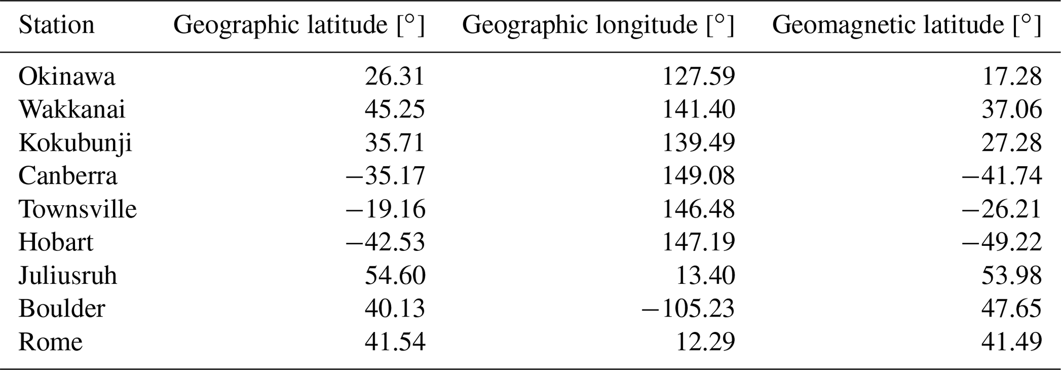
A key aspect in the present study is how IRI determines F2 parameters for a given location. To begin, foF2 is obtained from CCIR (Consultative Committee on International Radio) maps that are based on a procedure of numerical mapping of a set of coefficients (CCIR Atlas of Ionospheric Characteristics, 1991) determined from a fitting to observed monthly median foF2 data from a worldwide network of ionosonde stations (∼150 in total). From these coefficient maps, IRI reproduces the diurnal, seasonal, and solar activity variation of foF2 in terms of latitude and longitude through Fourier time series. First, there is a set of functions in terms of geographic coordinates and the modified dip latitude used to describe the variation of the Fourier coefficients for a given number of harmonics defining the diurnal variation. Then, the seasonal variation is taken into account through a set of these coefficients (988 in total) for every month of the year. Finally, the solar activity dependence is considered by having all these monthly coefficients for two different activity levels: IG12=0 and IG12=100. From a linear fit between these two extremes, the harmonic coefficients for any solar activity level can be estimated. IG was originally computed using 13 globally distributed ionosonde stations that included two of the nine stations here analyzed: Kokubunji and Canberra (Liu et al., 1983). The distribution of these stations was a compromise between good global coverage and reliable long-operating-period ionosonde stations. Due to station closures and data unavailability, the number of stations used in IG has decreased to four but still includes the two stations used in the present study (Brown et al., 2018). Therefore, this proxy, being obtained from ionospheric measurements, involves foF2 variations not covered by a solar index.
Specifically, when a given solar proxy is selected among the eight IRI-Plas options, it is automatically converted to other related indices used by the different modules' procedures (Gulyaeva et al., 2018). In this way, foF2 interannual variation is determined by IG12, since this index finally defines the CCIR coefficient values.
In the case of hmF2, we consider the default option, which corresponds to the AMTB-2013 model (standing for Altadill-Magdaleno-Torta-Blanch) (Altadill et al., 2013). This model is based on quiet ionosphere data from 26 digisondes collected between 1998 and 2006. The monthly averages of the global hmF2 variations are represented by spherical harmonics including modified dip latitude and longitude for two selected levels of Rz12 (0 and 100, as in the case of IG). The interannual variation of hmF2 is defined then by Rz12 since, for a given date, hmF2 is obtained from a linear fit of the spherical harmonic coefficients between Rz12=0 and 100 particularized for the corresponding Rz12 value. The same procedure is applied in the cases of the other two options for hmF2 modeling. Thus, the proxy used in this case, unlike the foF2 case, is only reflecting solar activity variability. Nevertheless, we include its long-term trend analysis considering that the correlation between IG and Rz is higher than 0.99 and that, for a given location and hour, foF2 and hmF2 interannual variation highly correlates. Moreover, IG correlates the highest with Rz exceeding 0.99 throughout the period 1960–2022. The linear correlation between IG and MgII, F10.7 and Lyman-α, for example, are 0.975, 0.985 and 0.970, respectively.
To assess foF2 and hmF2 trends, monthly values were obtained first from IRI-Plas. This model was run over a latitude–longitude grid, covering 90∘ N to 90∘ S and 180∘ E to 180∘ W, throughout the period 1960–2022, specifically at 00:00 and 12:00 LT, with the following inputs: (1) MgII as the solar activity proxy, (2) CCIR maps for foF2, (3) storm model off, and (4) AMTB-2013 model for hmF2. Considering just one day in the month or assessing the monthly median from all its daily values should give similar results due to the fact that the IRI model presents a smooth variation at daily timescale. Therefore, we considered foF2 and hmF2 values for the 15th day of each month as equivalent to the monthly median. Selecting other days or estimating all daily values within a month to assess the true median does not significantly affect the final results, as is discussed later in the Discussion section.
A total of series were obtained for foF2 and hmF2. In each case, annual mean series were constructed, together with series for each of the 12 months (that is, 13 series per grid point and per local time considered), all covering the period 1960–2022, which implies 63 points per series.
The foF2 and hmF2 filtering was made in the usual way by estimating the residuals from a linear regression with MgII as the solar extreme UV (EUV) proxy (Laštovička, 2021b, c), according to
where XIRI is the IRI modeled foF2 or hmF2 data, and A and B are the least square parameters of the linear regression between XIRI and MgII. The linear trend was assessed from the linear regression between these residuals and time; that is,
where t is in years, and α is the desired trend [MHz yr−1] for foF2 or [km yr−1] for hmF2. We will then have one α value for each grid point for the annual and for the 12 monthly series. Global means were also calculated in each case using a cosine (latitude) weighting.
The selection of MgII as the solar proxy input for IRI-Plas (and to filter foF2 and hmF2 variability linked to solar activity) is based on recent studies which recommend the use of this index as a solar proxy for foF2 trend estimations (Laštovička, 2021b, c; de Haro Barbas et al., 2021). We assume it is also the most adequate in the case of hmF2.
The MgII index was obtained from the University of Bremen. It is freely available at http://www.iup.uni-bremen.de/UVSAT/Datasets/MgII (last access: 12 September 2023) (Viereck et al., 2010; Snow et al., 2014). The extended time series was considered in order to cover the period before 1978.
To determine trends induced by Earth's magnetic field secular variation only, we also run IRI-Plas for fixed solar activity conditions by keeping Rz constant at a mean level while running the years from 1960 to 2022. Trends were assessed directly through Eq. (2). A previous filtering is not needed since the only foF2 and hmF2 time variations generated by the model are those linked to the slow changes of the modified dip at each location.
Only foF2 was considered in the comparison between IRI and experimental trend values. In order to assess the level of agreement between model and data, nine stations were chosen, which are listed in Table 1. Trends were evaluated using Eq. (1) to filter the solar activity effect and Eq. (2) to estimate trends in two ways: using the monthly median data, which will be called experimental trends (αexp), and the IRI-Plas model output, which will be called IRI trends (αIRI).
Table 1Geographic coordinates and geomagnetic latitude of the nine ionospheric stations analyzed to determine IRI foF2 trends accuracy.
The following metrics commonly used in data-model prediction comparisons (Willmott and Matsuura, 2005; Chicco et al., 2021) were considered to compare IRI to experimental trends: the mean relative error (MRE) and the mean absolute error (MAE). Their equations are
These parameters were assessed to determine overall IRI performance and also for each station separately. In the first case, summation is carried over the nine stations considering the annual mean series for 12:00 and 00:00 LT. In the second case, summation is carried out for each station over the 12 months.
MRE measures the average bias of IRI trends that are overestimating or underestimating the experimental trends depending on its sign: positive or negative, respectively. It gives similar information to the percentage bias, and its optimal value is 0. MAE is a scale-dependent measure of deviation that corresponds to the IRI trend deviations from experimental ones. The optimal value of MAE is 0, indicating that both trends are identical.
Monthly median foF2 data from the ionospheric stations were obtained as follows. Japanese and Australian station data are available from the National Institute of Information and Communications Technology, Japan (https://wdc.nict.go.jp/IONO/index_E.html, last access: 12 September 2023), and the World Data Centre (WDC) for Space Weather, Australia (https://downloads.sws.bom.gov.au/wdc/iondata/au/, last access: 12 September 2023), respectively. Both databases contain monthly medians updated to 2022. European station monthly medians up to 2009 were obtained from the Damboldt and Suessmann database (Damboldt and Suessmann, 2012) (https://downloads.sws.bom.gov.au/wdc/iondata/medians/, last access: 12 September 2023). In the case of Juliusruh, the period was updated until 2022 with monthly medians available from https://www.ionosonde.iap-kborn.de/mon_fof2.htm (last access: 12 September 2023). In the case of Boulder and Rome, the period was updated with data from the Lowell GIRO Data Center (LGDC) (Reinisch and Galkin, 2011). The foF2 from the Digital Ionogram Data Base (DIDBase) at LGDC has a frequency of 5 min. In order to obtain the monthly medians, we first selected data with autoscaling confidence score (CS) greater than 70 %, and then we estimated for each month the hourly median. In the case of these two stations, it was checked that the last 2 years available from the Damboldt and Suessmann database had a reasonable coincidence (within 95 %) with the data obtained from the other two sources.
5.1 foF2 and hmF2 trends based on the IRI model, as well as spatial variation patterns
Figure 1 shows foF2 and hmF2 trend values for 12:00 and 00:00 LT. The geomagnetic equator is also plotted for years 1960 and 2022. The foF2 trends are plotted in percent, which were estimated by dividing α into foF2 means along the complete period (1960–2022) at each grid point. In addition to overall negative trends in all cases, it can be noticed that the strongest trends occur in the region of the greatest geomagnetic equator displacement.
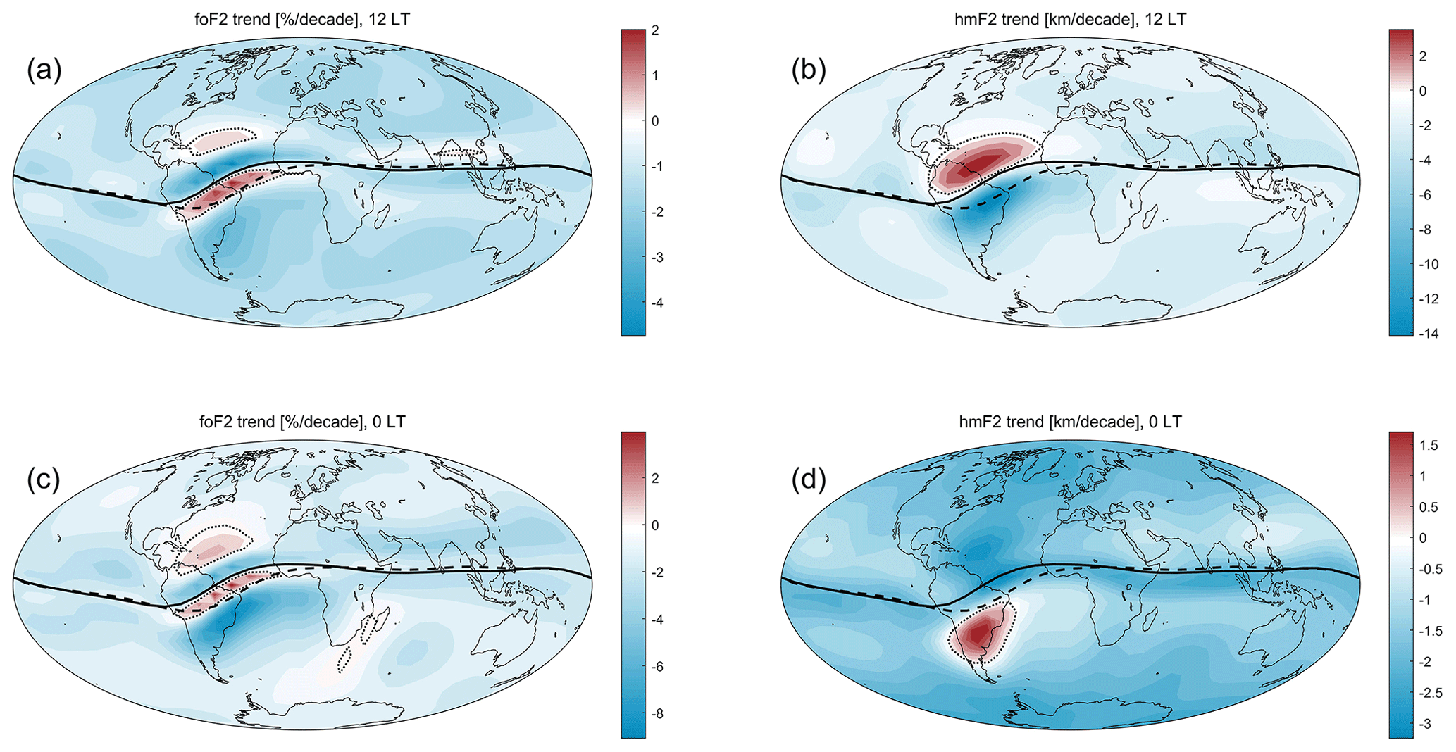
Figure 1Trends of foF2 (a, c) and hmF2 (b, d) at 12:00 LT (a, b) and 00:00 LT (c, d) throughout the period 1960–2022 assessed with the IRI outputs, which were previously filtered using Eq. (1). Note that trends are indicated per decade and that foF2 trends are in percent. Enhanced dashed and solid lines indicate the magnetic equator position in 1960 and in 2022, respectively. Dotted lines indicate zero trend.
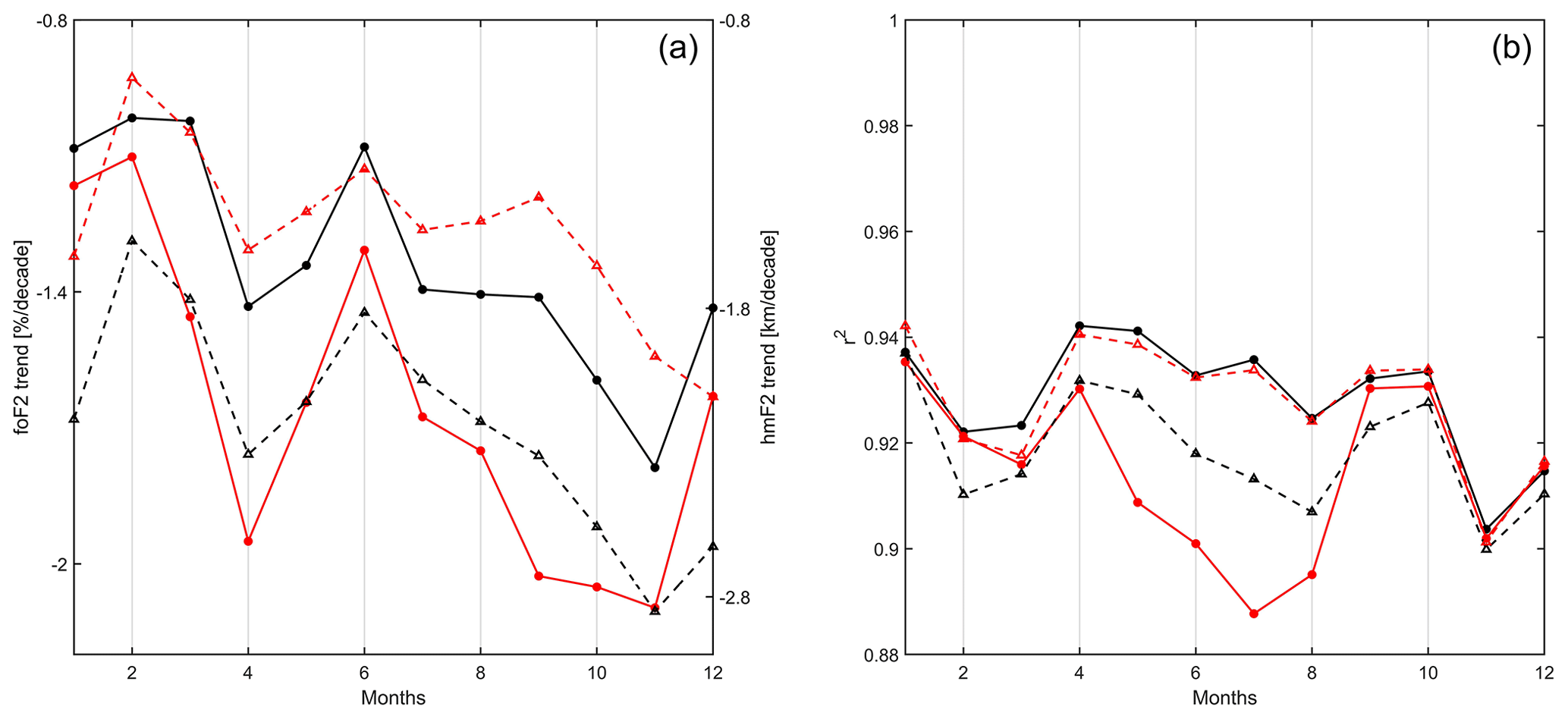
Figure 2Global mean values of the linear trends (a) and the squared correlation coefficient (r2) between each parameter and MgII (b) of foF2 (solid line with circles) and hmF2 (dashed lines with triangles) at 12:00 (in black) and 00:00 LT (in red).
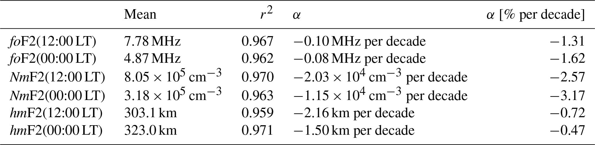
The global mean trends in each case are listed in Table 2, together with the mean values of F2-region parameters, to which the peak electron density, NmF2, was added in order to make some comparisons with other published results in the next section. Trends are listed in absolute and percentage values. The squared correlation coefficient, r2, of each parameter and MgII is also listed to indicate the quality of the fit to each regression model given by Eq. (1).
Table 2Global mean values, using a cosine (latitude) weighting, of F2-region ionospheric parameters, squared correlation coefficient (r2) of each parameter and MgII, linear trends of filtered parameters indicated in units per decade, and the same trends in percentage per decade.
Trends assessed for each month have a similar spatial pattern as the annual trends shown in Fig. 1, even though they are not identical. Figure 2 (left panel) shows the global mean trend values from January to December. Weaker global trends are noticed in February and in June. Something to notice is the decrease of r2 of the fit to filter solar activity, shown in Fig. 2 (right panel). All values are lower than the annual case. This would be due to the variation of foF2 and hmF2 associated with solar activity being efficiently described by the 12-month moving average of a solar proxy. When analyzing the time series corresponding to each month separately, considering the unsmoothed monthly values lower r2 because the inter-monthly variation is not eliminated. As an additional comment, in general, when considering solar EUV proxies, they are all more alike when the time series compared consist of annual means rather than monthly or daily means. This is because, at these shorter timescales, each time series conserves distinct variability patterns that are erased when annual or 12-month running means are used.
Figure 3 shows trends for IRI-Plas run keeping Rz constant at a mean level (Rz=70). These trends result, then, from the Earth's magnetic field secular variation only since they reflect the modified dip changes at each location. From a comparison with Fig. 1 trend values and spatial patterns, two things become clear: (1) the positive and negative trend spatial configuration is due to the magnetic field variation, and (2) the overall negative trends, away from the region with the pronounced geomagnetic field equator displacement throughout the period considered, are not due to the magnetic field effect. Global mean trends in the case of Fig. 3 are −0.0004 MHz per decade and −0.086 km per decade. In percentage they become −0.0006 % per decade and −0.023 % per decade, respectively. When comparing these values with those listed in Table 2 for 12:00 LT, it could be said that the global mean trend driven by the Earth's magnetic field, despite being relatively strong at some regions, averages essentially to zero. The foF2 and hmF2 global means in this case are 7.93 MHz and 308.6 km, similar to the Table 2 values.
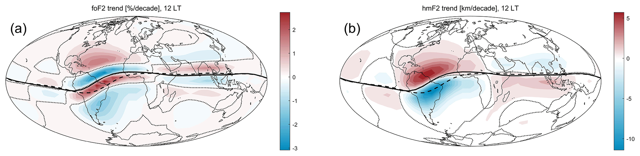
Figure 3Trends of foF2 (a) and hmF2 (b) at 12:00 LT throughout the period 1960–2022 assessed with the IRI outputs using Eq. (1), without previously filtering. Note that trends are indicated per decade, and foF2 trends are in percent. Enhanced dashed and solid lines indicate the magnetic equator position in 1960 and in 2022, respectively. Dotted lines indicate zero trend.
5.2 Agreement between IRI and experimental trends for selected stations
Figures 4 and 5 show experimental and IRI foF2 trends for each of the nine stations, at 12:00 and 00:00 LT, respectively, in terms of months. Error bars are estimated as 1σ. Generally good agreement can be noticed, which is evinced by MAE and MRE values listed in Table 3, in particular for the 12:00 LT case. Annual experimental and IRI trends are listed in Table 4.
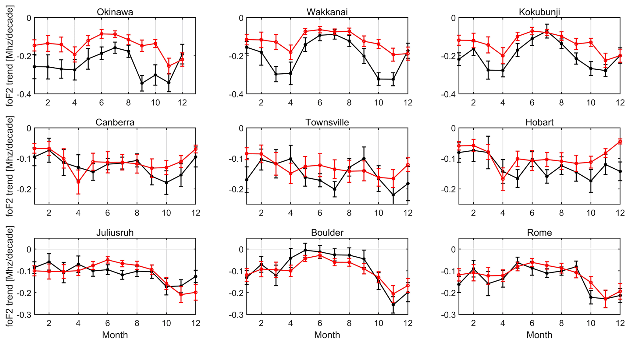
Figure 4Monthly variation of foF2 trends [MHz per decade], at 12:00 LT, estimated with experimental data (black) and with the IRI-Plas model (red). Error bars correspond to 1 standard deviation.
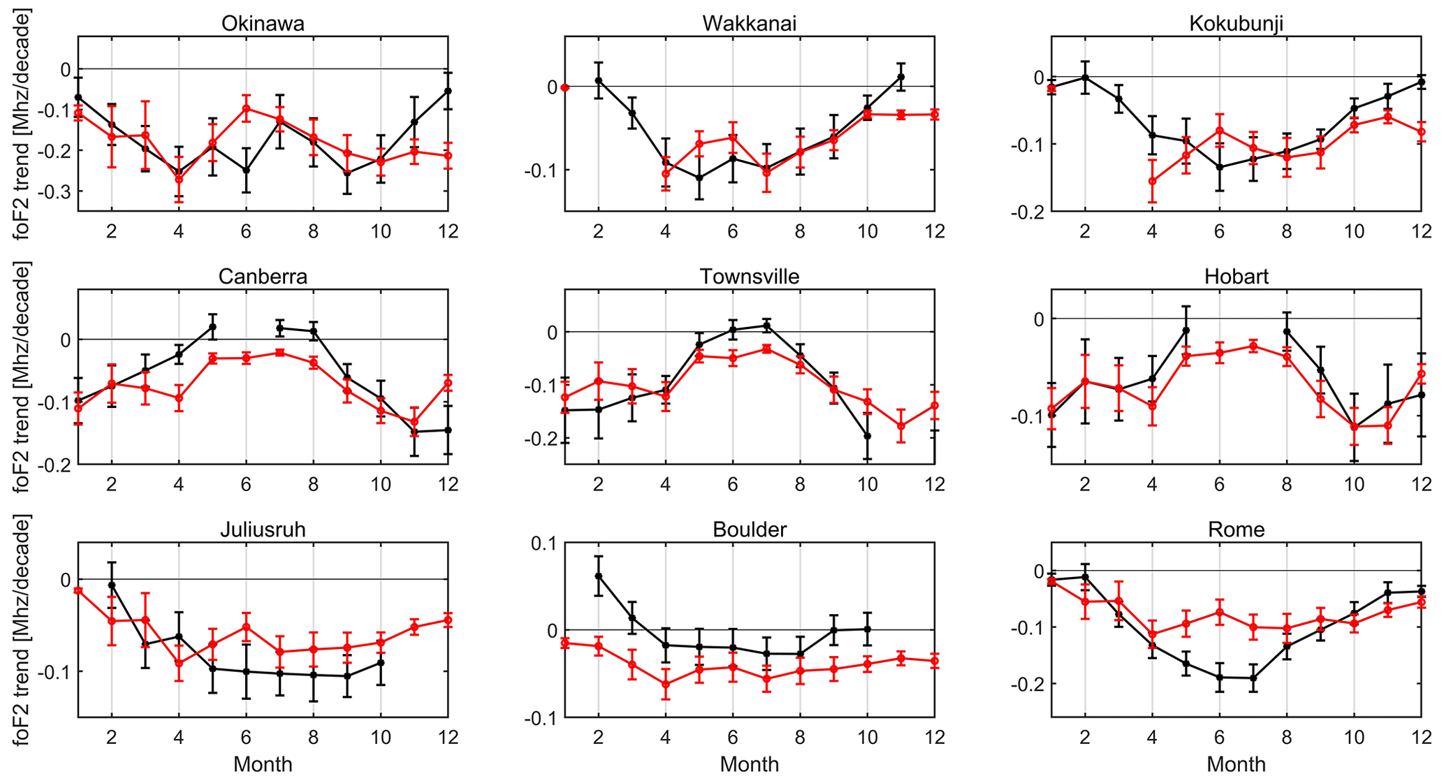
Figure 5Monthly variation of foF2 trends [MHz per decade], at 00:00 LT, estimated with experimental data (black) and with the IRI-Plas model (red). Error bars correspond to 1 standard deviation.
Table 3The foF2 trends assessed with experimental data and with the IRI-Plas model, considering annual mean data series at 12:00 and 00:00 LT. The last rows present the MAE and MRE between these trends carried over the nine stations. MRE* corresponds to MRE without the stations of highest relative error; that is, Okinawa in the 12:00 LT case and Boulder in the 00:00 LT case.
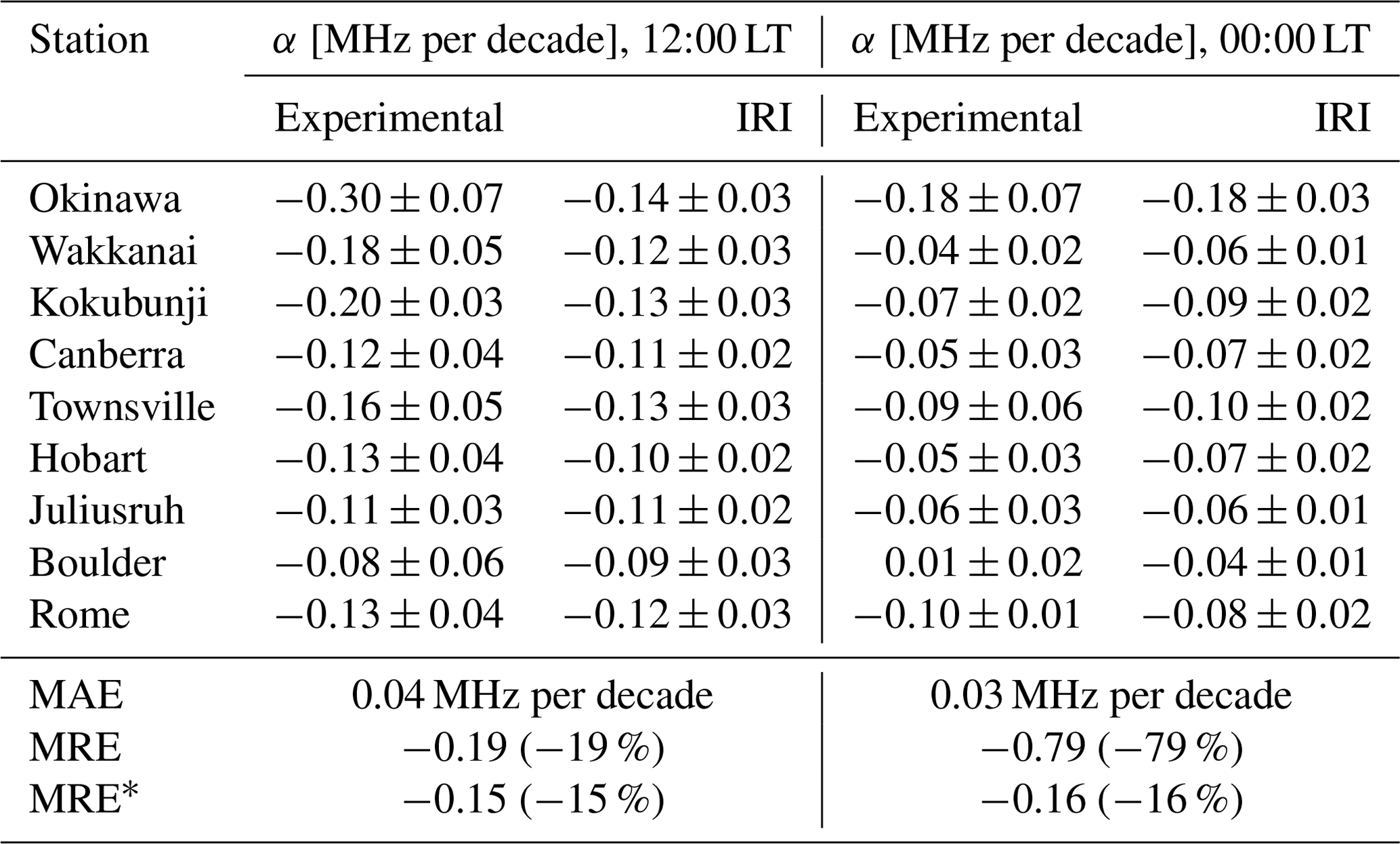
Table 4MAE and MRE of foF2 trends assessed with experimental data and with the IRI-Plas model, considering monthly data series at 12:00 and 00:00 LT, for each station. MRE values between round brackets correspond to estimations excluding experimental trends equal to zero within the error.
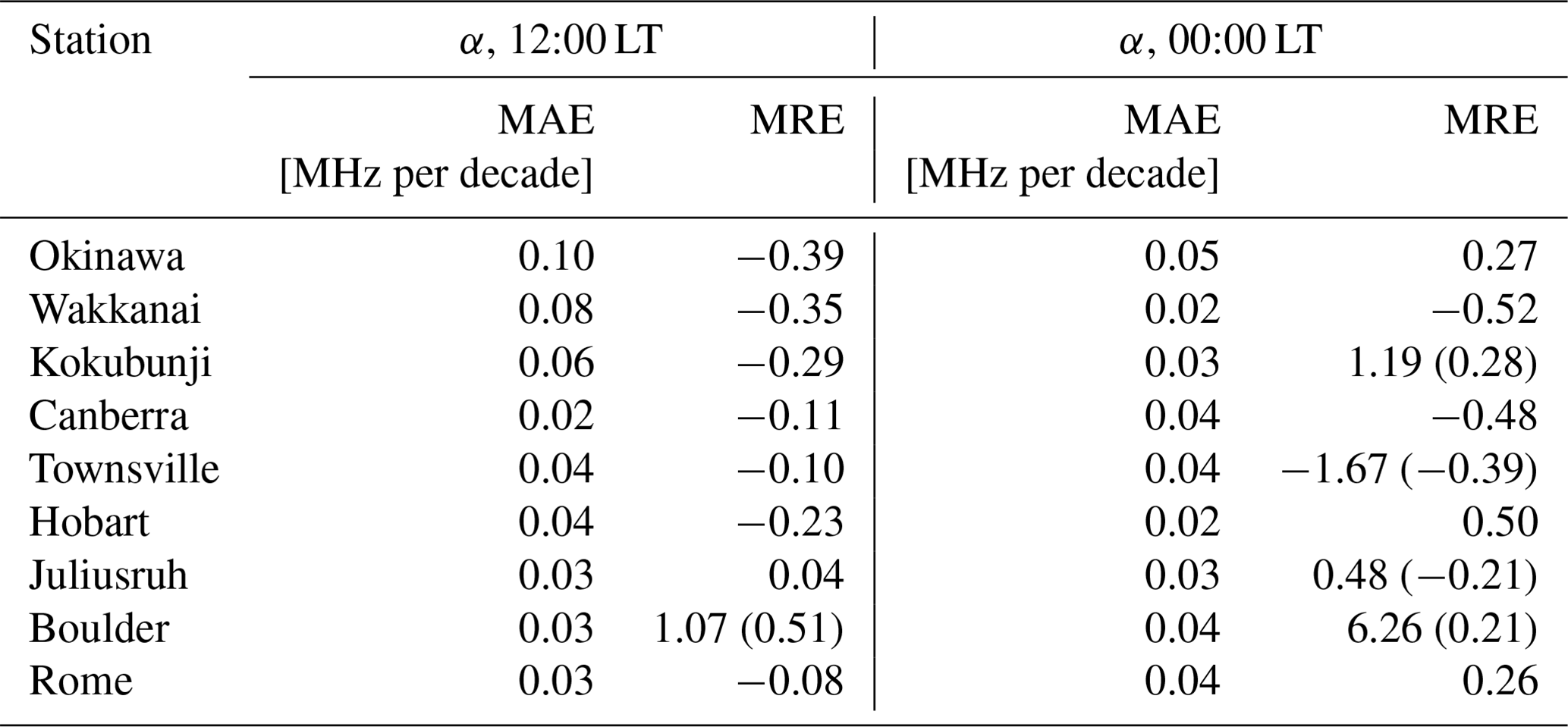
The cases with large MRE values correspond to those stations and local times that have an experimental trend value very close to zero. Since this value appears in the denominator of MRE (see Eq. 3), even a small difference in the numerator leads to a large MRE. However, we can re-estimate MRE values excluding experimental trends equal to zero within the error. Specifically, in the 12:00 LT case, these would correspond to experimental trend values for Boulder in May. In the 00:00 LT case, these would correspond to Kokubunji in February and December, Townsville in June, Juliusruh in February, and Boulder in September and October. By doing so, the MRE decreases, as indicated by the values presented within round brackets in Table 4.
The Whole Atmosphere Community Climate Model eXtension (WACCM-X) has been run to assess trends in the upper atmosphere (Solomon et al., 2018; Cnossen, 2020) and some results can be analyzed comparatively with the mean global trends here obtained with IRI-Plas, as well as the spatial variation of the trends.
WACCM-X is a general circulation and complex model with high-resolution modeling capabilities, which incorporates a comprehensive set of physics processes to estimate a more realistic representation of the atmospheric (and ionospheric) status, including chemical, dynamical, and radiative processes. This model is coupled with several Earth systems, making it easy to analyze the weighting of any change in trends, e.g., the increase of a particular component in atmospheric composition. The trend results obtained by Solomon et al. (2018) and by Cnossen (2020) with WACCM-X that can be compared with those of IRI-Plas are listed in Table 5.
Table 5Comparison between IRI-Plas and WACCM-X results from Solomon et al. (2018) and Cnossen (2020). All values correspond to global means throughout the period analyzed in each case, with the exception of NmF2 and hmF2 mean values which correspond to global means along solar minimum activity level periods.
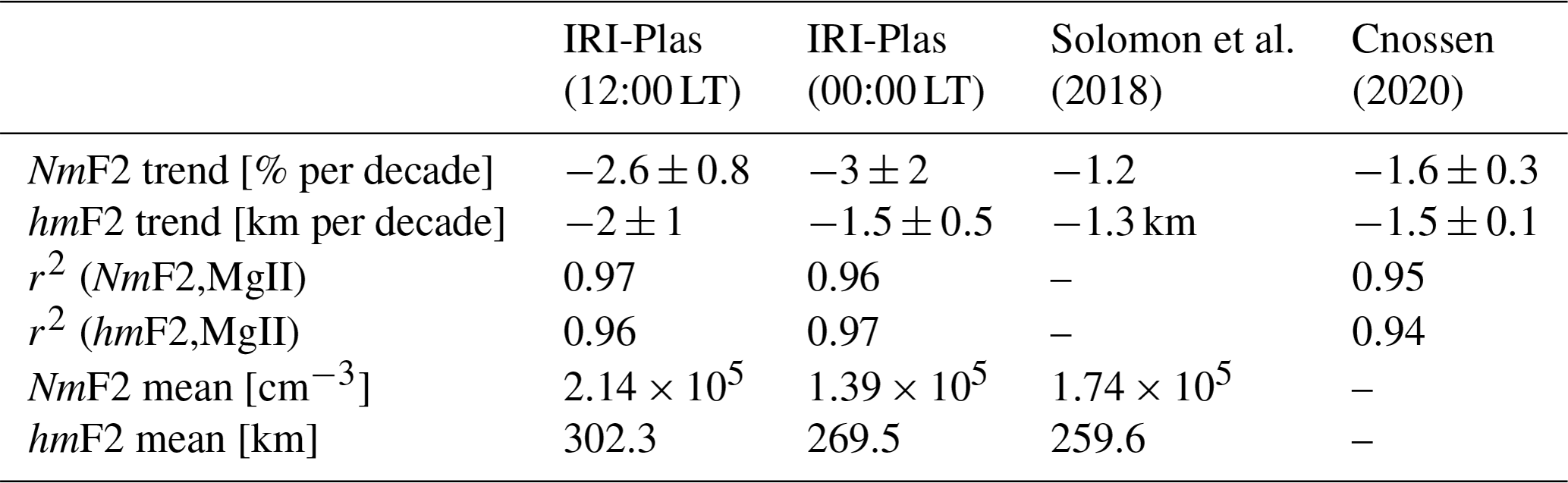
In the case of Solomon et al. (2018), global mean values are presented considering only minimum solar activity level and solar quiet conditions, with which no filtering is needed before the trend assessment. The period considered is 1972–2005, and there is no local time consideration, so we will assume that their values could be compared to the mean of our 12:00 and 00:00 LT values. Their trends are weaker than assessed with IRI-Plas, even if we reassess trends considering 1972–2005 instead of 1960–2022. In both cases, trends are negative, but the NmF2 trend they obtain is around half the IRI-Plas trend, as can be deduced from Table 5. In addition to trend values, NmF2 and hmF2 mean global values estimated by Solomon et al. (2018) can be compared to IRI-Plas output averages considering only years around solar minimum activity levels out of the 1960–2022 period. In this case, the results are similar for NmF2, but for hmF2 their mean value is lower than that obtained with IRI-Plas.
Cnossen (2020) presents the global mean values, as in the previous case, and the spatial pattern variation. Our trend estimation methodology is similar to “Model 1”, which includes terms for only solar activity and a long-term trend, with two differences: F10.7 is used instead of MgII as solar proxy, and the trend term is included in a multiple regression together with the solar activity term. The differences due to methodologies are not expected to be significant (Laštovička et al., 2006). Absolute values of trends in this case are slightly higher than in Solomon et al. (2018) but again lower than those of IRI-Plas, with the greatest difference in the NmF2 trend case, as can be noticed from Table 5. The squared correlation coefficient, that indicates the quality of the fit to each regression model given by Eq. (1), is similar in all the cases.
Is important to remark that the trends reported by Solomon et al. (2018) may have resulted in lower values because they run the simulation with constant low solar activity. This would have neglected part of the trend that may be induced by the solar EUV flux negative trend along the last minima periods and which we consider partly responsible for the overall negative trends observed in measured ionospheric data.
The spatial variation pattern can also be compared. In the case of hmF2, the Cnossen (2020) spatial pattern is consistent with the IRI-Plas trends at 12:00 LT, with overall negative trends and a positive patch above the geomagnetic equator between Africa and South America. This would be in agreement with the trend expected from the northward geomagnetic equator secular displacement, which is strongest in this region, and assuming that the equatorial ionization anomaly (EIA) pattern of hmF2 moves along with this displacement. The highest decreasing trends are observed consequently below this positive patch, in response to the northward movement of hmF2 highest values. With respect to trend values, the strongest positive trends seem similar, around 2 km per decade. However, the highest negative trends are greatest in the IRI-Plas case, reaching values of 12 km per decade at noontime, while in the Cnossen (2020) case this value corresponds to 5 km per decade.
In the case of hmF2 trends at 00:00 LT, hmF2 presents a trough, even though not as well defined as the crest during daytime hours. The displacement of this trough attached to the geomagnetic field northward displacement induces an effect inverse to that during noon. That is, a positive trend patch appears below it, with the strongest negative trends above.
A similar situation occurs with the foF2 trend spatial pattern. In order to compare the trend values in percent with those of NmF2, they should be multiplied by 2. This means that our strongest negative trend is again the highest. The spatial pattern here has alternating bands of positive and negative trend values aligned with the EIA, which can be explained in terms of the EIA displacement following the geomagnetic equator. Between ∼60∘ W and 0∘ in longitude, the equator shift is the greatest and northward, so this is the region where the strongest alternating trends are noticed (Elias et al., 2022). This longitudinal extension is narrower than in the Cnossen (2020) case, who detect it between W and E. A notorious difference is that between the initial and the final position of the geomagnetic equator in this longitudinal range, Cnossen (2020) detects a negative trend band, while in our case a positive band is observed.
This difference may be caused by a poor resolution in latitude. In order to see the trend bands expected in the region between the initial and final position of the equator, a schematic plot is shown in Fig. 6a of the EIA foF2 trough in its initial and its final position in 1960 and 2022, respectively. In this figure, it can be clearly noticed that the region between these positions will present a positive portion followed by a negative one. The first one corresponds to the region with low foF2 in 1960, which has now become a region with higher foF2 values (since the trough has moved). The second one corresponds to a region of higher foF2 in 1960, which now is located under the EIA trough. On average, the geomagnetic equator has displaced ∼5 to 10∘ in the region's strongest shift, so for low resolutions, the grid points may coincide with one of either trend bands. This could partly explain the difference between the Cnossen (2020) negative band between the equator positions and our corresponding positive band. Figure 6b shows an enlarged portion of the trend's spatial pattern obtained with IRI-Plas but increasing the latitude resolution to 1∘, where a positive and a negative band within the limits of the 1960 and the 2022 equator positions can be noticed.
The spatial pattern linked to the EIA displacement following the geomagnetic equator and clearly isolated in Fig. 3 is expected in IRI-Plas foF2 and hmF2 modeling since the model includes a real geomagnetic field. Even though there are very few stations along its location, the IRI model reproduces the EIA pattern through the variation in the magnetic inclination, obtained from IGRF, on which interpolation coefficients depend.
It is worth noting that in very recent studies, the 30 cm solar flux index, F30 (available at https://spaceweather.cls.fr/services/radioflux/, last access: 12 September 2023), is identified as the most suitable EUV solar proxy for filtering foF2 to subsequently estimate long-term trends, followed by MgII (Laštovička and Burešová, 2023). We also conducted a recent study (Zossi et al., 2023) where we concluded that both F30 and MgII are equally appropriate but without being able to distinguish which one is better of the two. In the present work, we did not consider F30 because IRI-Plas does not have this option. However, we compared the trend values for the nine stations here analyzed, from measurements and IRI-Plas model, considering each of these indices to filter solar activity effect, and, while we did not obtain identical values, they are in strong agreement. This agreement is nearly complete in terms of sign and practically within the error range of the trends in terms of values. Nevertheless, this deserves a detailed comparative analysis and could possibly suggest the inclusion of F30 as an additional index to the options already available in this model.
Another important aspect concerns IG and Rz long-term trends. The explained variance of each of these proxies by MgII is ∼95 % (r2×100) in both cases (IG vs. MgII and Rz vs. MgII), and if the solar activity effect is filtered from them through the same linear regression as that performed on F2 parameters, negative trends are obtained in both residuals as is shown in Fig. 7. The decreasing trend observed in IG when filtered with MgII is mainly due to the last two solar cycle minima which are much lower than the previous two in the IG case (and also in the Rz case) than in the MgII case. This is due to the fact that the solar EUV flux during the last two minima has been lower than the values indicated by solar proxies. This would also induce a decreasing trend in foF2 (and in hmF2) which might be connected to the inadequate performance of the proxy in capturing the variations in solar EUV flux (Emmert et al., 2010; Chen et al., 2011; Bruevich and Bruevich, 2019; Elias et al., 2023). However, this is a topic for further research.
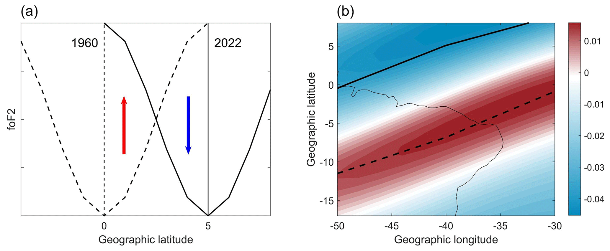
Figure 6(a) Schematic representation of the foF2 latitudinal profile around the EIA trough in 1960 (dashed line), centered in the magnetic equator in 1960 (vertical dashed line at latitude=0), and in 2022 (solid line), centered in the magnetic equator in 2022 (vertical solid line at latitude=5). The red arrow indicates the foF2 increase that would be observed in latitudes between 0 and ∼2.5, and the blue arrow indicates the decrease between ∼2.5 and 5. (b) The foF2 trend along 1960–2022 assessed with IRI-Plas (solar activity filtering with MgII) in the region with the largest equator displacement with an increased resolution: latitude–longitude grid. Enhanced dashed and solid lines indicate the magnetic equator position in 1960 and in 2022, respectively.
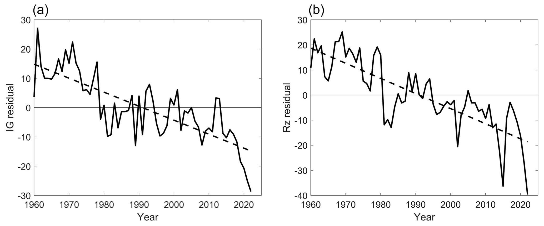
Figure 7Residuals of the linear regression between annual means IG and MgII (a) and Rz and MgII (b).
Another aspect to discuss is the use of foF2 and hmF2 values for a single day of each month as representative of the monthly median. On the one hand, as mentioned in Sect. 3, the IRI model, with the “storm off” option, exhibits a smooth daily variation throughout each month. To analyze the impact of choosing this particular day on the trend instead of the monthly median or mean obtained from all daily values, we assessed annual noon foF2 trends for a mid-latitude location (20∘ N, 30∘ E), considering other days of each month (but using the same day for every month and year). We also assessed the trends by considering the median and the mean value of each month. Even though the trend values are not the same, the difference between any of them is around ∼0.006 MHz per decade, which is smaller than the trends' standard error (∼0.02 MHz per decade). As an additional possibility, we considered using a random day in each month. For example, for the year 1960, we used day 12 for January, day 27 for February, day 5 for March, and so on, for the following months and years. From 10 000 random estimations we made, the minimum trend value obtained is −0.09 MHz per decade, and the maximum value is −0.13 MHz per decade. Both include within the error interval (±0.02 MHz per decade) the value of the trend obtained considering day 15 (which is −0.0110 MHz per decade) and that considering the true foF2 median (which is −0.0111 MHz per decade). The most probable trend values in this running of 10 000 trend estimations lies between −0.111 and −0.109, and it again includes the value estimated in this work considering day 15.
An additional topic deserving further research is the global picture easily obtained with IRI of the geomagnetic field secular variation-induced trends. We will not go deeper into this aspect in this work, but we considered it important to mention that the positive and negative trend patches are consistent with the results by Cnossen and Richmond (2012), who analyzed the effect of the Earth's dipole inclination variation using the Coupled Magnetosphere-Ionosphere-Thermosphere (CMIT) model. The only difference is that they show the effect of a dipole axis increasing its inclination, and the secular variation observed during the last decades is consistent with a dipole aligning with the rotation axis. That is why, in a rough comparison, the sign of the trend's patches in Fig. 3 are opposite to those of Fig. 7 (lower panels) of Cnossen and Richmond (2012). This is something worth exploring, using IRI, at least as long as the field remains mainly dipolar.
Considering how the foF2 and hmF2 interannual variation is determined in IRI-Plas (and in other IRI model versions), it can be argued that the overall negative trends are due to the same long-term trend occurring in IG and Rz.
For foF2, the attribution to external forcings other than the magnetic field is clear since IG carries the information of foF2 measurements. Thus, we can expect that the trends obtained could be a reasonable approach to experimental trends. In fact, this index includes the variability by other sources affecting the ionospheric F2 layer, like the greenhouse gas concentration increases or other neutral composition changes or dynamical disturbances. It does not include, however, the magnetic field secular variation effect since it averages to almost zero. Hence, the foF2 trends obtained using IRI-Plas model values can be, to a first approximation, attributed to the greenhouse cooling effect plus the secular variation in Earth's magnetic field. This, of course, assumes that the dominant driver behind the global declining foF2 trend, and of IG, is indeed the greenhouse effect. In addition, to verify this in a more localized spatial scale, we were able to compare foF2 trends, considering annual and monthly series, determined with experimental data from nine mid-latitude stations and with the corresponding IRI-Plas modeled values. We obtained a reasonable agreement, with average differences of ∼20 %. Something to argue is that by using mid-latitude stations, we use the stations for which IRI surely works best.
On the other hand, hmF2 trends result from the Rz overall decreasing trend when it is filtered with MgII (or any other solar EUV proxy). Even though the values are coherent with expected trends due to greenhouse cooling (due to the fact that Rz varies almost identically to IG), we cannot conclude, using IRI, that its long-term lowering is due to greenhouse gas concentration increases. This is due to the coincidence that both hmF2 from IRI and hmF2 from measurements and theoretical considerations are forced by a mechanism inducing a downward trend; in the first case, it is the Rz overall downward trend throughout the period considered, while in the latter it would be due to the greenhouse effect. In addition, of course, the downward trend in Rz has nothing to do with the increasing concentrations of greenhouse gases during the last decades. They both just happen to be in the same direction. Despite this, it is considered worthwhile to compare these trends with experimental values as a future task. Smaller Rz values since ∼2001 have been mentioned some years ago by Lukianova and Mursula (2011) and Mielich and Bremer (2013).
To be able to attribute observed trends in IRI to processes unrelated to solar activity, it would be valuable to consider two potential approaches:
-
The first is interpolation of the CCIR maps with “effective indices” derived from data, as already proposed by Pignalberi et al. (2018). This would be similar to the approach used for IG. By using effective indices based on observed data, time variations not directly tied to solar activity would be accounted for.
-
The second is interpolation from annual CCIR maps, instead of the two maps currently used. This would involve updating the CCIR maps on an annual basis, assimilating the most recent and accurate data; thus, the time variation obtained would not result exclusively from solar activity variability.
Compared to a more theoretically based model, it is important to remark that IRI-Plas is designed for modeling a specific atmospheric sub-region, namely, the ionosphere, whereas WACCM-X is a global circulation model that simulates the entire atmosphere. Thus, an advantage of this model is that, in considering coupling processes among several Earth systems, it allows one to analyze the weighting of any change in trends, e.g., the increase of a particular component in atmospheric composition. Nevertheless, the negative side of general circulation models is the substantial computational resources and time needed to run simulations, being almost exclusive for high-performance computing centers. In the case of IRI, a great advantage is its user-friendly design, allowing it to be run on modest computers consuming few resources with extremely short computational times (on the order of minutes), while still being a reliable tool to get an approximated status of the ionosphere. On the other hand, this reference model adopts simplified assumptions and parameterizations to represent complex ionospheric processes.
Before summarizing the answer to the question raised by this study's title, we bring up again some recommendations for future tasks suggested throughout this work: (1) a comparison between hmF2 trends at specific locations between IRI and ionosonde data, similar to foF2 analysis; (2) the spatial pattern of IRI trends due only to the Earth's magnetic field and its comparison with complex models with theoretical approaches; (3) the correct attribution of the general foF2 and hmF2 downward trend: the greenhouse affect or a long-term decreasing EUV flux not shown by EUV proxies which are used to filter solar activity effect since Rz was suggested to be discarded for this purpose (Mielich and Bremer, 2013); and (4) to modify IRI effective proxies or coefficient maps in order to determine foF2 and hmF2 interannual variations that include external sources other than solar activity only.
In summary, regarding the question set forth in this study's title, we conclude that the IRI model can be a valuable tool for obtaining preliminary approximations of experimental trends, at least in the case of foF2. This is particularly significant given the low spatial density of data and the scarcity of time series with sufficient length to estimate trends. In the case of hmF2, there would be an added advantage considering that, while foF2 is an accurately measured parameter, hmF2 is often missing or derived from the proxy M(3000)F2 parameter. However, even if hmF2 trends obtained with IRI-Plas are close to the expected values, they are linked to different drivers.
The IRI-Plas code is freely available from the IZMIRAN Ionospheric Weather server at https://www.izmiran.ru/ionosphere/weather/grif/SPIM/ (last access: 12 September 2023, Gulyaeva et al., 2011). The IRI 2016 and 2020 versions, also used in this work, were run from the HF (high-frequency) propagation toolbox, PHaRLAP, created by Manuel Cervera, Defence Science and Technology Group, Australia (manuel.cervera@dst.defence.gov.au), available at https://www.dst.defence.gov.au/our-technologies/pharlap- provision-high-frequency-raytracing-laboratory-propagation-studies (last access: 12 September 2023). This toolbox is available by request from its author. The foF2 data from Japanese and Australian stations are available at https://wdc.nict.go.jp/IONO/index_E.html (last access: 12 September 2023, WDC for Ionosphere and Space Weather, 2023), and https://downloads.sws.bom.gov.au/wdc/iondata/au/ (last access: 12 September 2023, Australian Space Weather Forecasting Centre, 2023a), respectively. Boulder and Rome foF2 data were obtained from https://downloads.sws.bom.gov.au/wdc/iondata/medians/ (last access: 12 September 2023, Australian Space Weather Forecasting Centre, 2023b) and https://doi.org/10.5047/eps.2011.03.001 (Reinisch and Galkin, 2011). Juliusruh foF2 data are available from https://www.ionosonde.iap-kborn.de/mon_fof2.htm (last access: 12 September 2023, Leibniz Institute of Atmospheric Physics at the University of Rostock, 2023). The MgII index is freely available at http://www.iup.uni-bremen.de/UVSAT/Datasets/MgII (last access: 12 September 2023, Viereck et al., 2010; Snow et al., 2014), IG is from https://www.ukssdc.ac.uk/cgi-bin/wdcc1/secure/geophysical_parameters.pl (last access: 12 September 2023, UK Solar System Data Centre, 2023), and Rz is from https://www.sidc.be/SILSO/datafiles (last access: 12 September 2023, WDC-SILSO, 2023).
BSZ: conceptualization, supervision, investigation, formal analysis, methodology, and writing; TD: investigation, methodology, validation, review and editing; FDM, BFdHB and YM: investigation, validation, review and editing; AGE: original draft preparation, investigation, formal analysis, review and editing.
The contact author has declared that none of the authors has any competing interests.
Publisher's note: Copernicus Publications remains neutral with regard to jurisdictional claims made in the text, published maps, institutional affiliations, or any other geographical representation in this paper. While Copernicus Publications makes every effort to include appropriate place names, the final responsibility lies with the authors.
This article is part of the special issue “Long-term changes and trends in the middle and upper atmosphere”. It is a result of the 11th International Workshop on Long-Term Changes and Trends in the Atmosphere, Helsinki, Finland, 23–27 May 2022.
Bruno S. Zossi, Franco D. Medina, Blas F. de Haro Barbas, and Ana G. Elias acknowledge research project PIP 2957. Trinidad Duran acknowledges research projects PICT 2019-03491 and PGI 24/F083. We are very grateful to David Themens for his comments on our article and for having the time for a fruitful and helpful discussion which helped greatly to improve the paper. We also gratefully acknowledge two anonymous reviewers for their valuable and insightful comments.
We acknowledge the International Reference Ionosphere (IRI) working group and the Defence Science and Technology Group (DST) of Department of Defence, Commonwealth of Australia, for providing the HF propagation toolbox, PHaRLAP, created by Manuel Cervera, from which IRI 2016 and 2020 were run. We acknowledge IONOLAB (http://www.ionolab.org/, last access: 12 September 2023) and the IZMIRAN Ionospheric Weather server (https://www.izmiran.ru/services/iweather/, last access: 12 September 2023) for providing IRI-Plas software. We also acknowledge GIRO data resources http://spase.info/SMWG/Observatory/GIRO (last access: 12 September 2023); the WDC for Ionosphere and Space Weather, Tokyo; National Institute of Information and Communications Technology; the Australian Space Weather Forecasting Centre (ASWFC); and the Leibniz Institute of Atmospheric Physics for providing foF2 data.
This research has been supported by the Consejo Nacional de Investigaciones Científicas y Técnicas (grant no. PIP 2957) and the Fondo para la Investigación Científica y Tecnológica (grant no. PICT 2019-03491).
This paper was edited by John Plane and reviewed by two anonymous referees.
Altadill, D., Magdaleno, S., Torta, J. M., and Blanch, E.: Global empirical models of the density peak height and of the equivalent scale height for quiet conditions, Adv. Space Res., 52, 1756–1769, https://doi.org/10.1016/j.asr.2012.11.018, 2013.
Australian Space Weather Forecasting Centre: Index of /wdc/iondata/au, [data set], https://downloads.sws.bom.gov.au/wdc/iondata/au/ (last access: 12 September 2023), 2023a.
Australian Space Weather Forecasting Centre: Index of /wdc/iondata/medians, [data set], https://downloads.sws.bom.gov.au/wdc/iondata/medians/ (last access: 12 September 2023), 2023b.
Bilitza, D., Pezzopane, M., Truhlik, V., Altadill, D., Reinisch, B. W., and Pignalberi, A.: The International Reference Ionosphere model: A review and description of an ionospheric benchmark, Rev. Geophys., 60, e2022RG000792, https://doi.org/10.1029/2022RG000792, 2022.
Brown, S., Bilitza, D., and Yigit, E.: Ionosonde-based indices for improved representation of solar cycle variation in the International Reference Ionosphere model, J. Atmos. Sol.-Terr. Phy., 171, 137–146, https://doi.org/10.1016/j.jastp.2017.08.022, 2018.
Bruevich, E. and Bruevich, V.: Long-term trends in solar activity. Variations of solar indices in the last 40 years, Res. Astron. Astrophys., 19, 090, https://doi.org/10.1088/1674-4527/19/7/90, 2019.
Cander, L. R.: Space Weather Causes and Effects, in: Ionospheric Space Weather, L.R. Cander, Springer Geophysics, Springer, Cham, 29–58, https://doi.org/10.1007/978-3-319-99331-7_3, 2019.
CCIR Atlas of Ionospheric Characteristics: Report 340-6, International Telecommunication Union (ITU), Geneve, http://handle.itu.int/11.1004/020.1000/4.283.43.en.1039 (last access: 12 September 2023), 1991.
Chen, Y. D., Liu, L. B., and Wan, W. X.: Does the F10.7 index correctly describe solar EUV flux during the deep solar minimum of 2007–2009?, J. Geophys. Res.-Space, 116, A04304, https://doi.org/10.1029/2010JA016301, 2011.
Chicco, D., Warrens, M. J., and Jurman, G.: The coefficient of determination R-squared is more informative than SMAPE, MAE, MAPE, MSE and RMSE in regression analysis evaluation, PeerJ Computer Science, 7, e623, https://doi.org/10.7717/peerj-cs.623, 2021.
Cnossen, I.: Analysis and attribution of climate change in the upper atmosphere from 1950 to 2015 simulated by WACCM-X, J. Geophys. Res., 125, e2020JA028623, https://doi.org/10.1029/2020JA028623, 2020.
Cnossen, I. and Richmond, A. D.: How changes in the tilt angle of the geomagnetic dipole affect the coupled magnetosphere-ionosphere-thermosphere system, J. Geophys. Res., 117, A10317, https://doi.org/10.1029/2012JA018056, 2012.
Damboldt, T. and Suessmann, P.: Consolidated Database of Worldwide Measured Monthly Medians of Ionospheric Characteristics foF2 and M(3000)F2, INAG (Ionosonde Network Advisory Group) Bulletin 73, https://www.ursi.org/files/CommissionWebsites/INAG/web-73/2012/damboldt_consolidated_database.pdf (last access: 12 September 2023), 2012.
de Haro Barbas, B. F., Elias, A. G., Venchiarutti, J. V., Fagre, M., Zossi, B. S., Tan Jun, G., and Medina, F. D.: MgII as a Solar Proxy to Filter F2-Region Ionospheric Parameters, Pure Appl. Geophys., 178, 4605–4618, https://doi.org/10.1007/s00024-021-02884-y, 2021.
Elias, A. G., de Haro Barbas, B. F., Zossi, B. S., Medina, F. D., Fagre, M., and Venchiarutti, J. V.: Review of Long-Term Trends in the Equatorial Ionosphere Due the Geomagnetic Field Secular Variations and Its Relevance to Space Weather, Atmosphere, 13, 40, https://doi.org/10.3390/atmos13010040, 2022.
Elias, A. G., Martinis, C. R., de Haro Barbas, B. F., Medina, F. D., Zossi, B. S., Fagre, M., and Duran, T.: Comparative analysis of extreme ultraviolet solar radiation proxies during minimum activity levels, Earth Planet. Phys., 7, 1–8, https://doi.org/10.26464/epp2023050, 2023.
Emmert, J. T., Lean, J. L., and Picone, J. M.: Record-low thermospheric density during the 2008 solar minimum, Geophys. Res. Lett., 37, L12102, https://doi.org/10.1029/2010GL043671, 2010.
Gulyaeva, T. and Bilitza, D.: Towards ISO Standard Earth Ionosphere and Plasmasphere Model, New Developments in the Standard Model, edited by: Larsen, R. J., Nova Science Publishers, New York, ISBN 978-1-61209-989-7, 2012.
Gulyaeva, T. L., Arikan, F., and Stanislawska, I.: Inter-hemispheric imaging of the ionosphere with the upgraded IRI-Plas model during the space weather storms, Earth Planets Space, 63, 929–939, https://doi.org/10.5047/eps.2011.04.007, 2011.
Gulyaeva, T. L., Arikan, F., Sezen, U., and Poustovalova, L. V.: Eight proxy indices of solar activity for the International Reference Ionosphere and Plasmasphere model, J. Atmos. Sol.-Terr. Phy., 172, 122–128, https://doi.org/10.1016/j.jastp.2018.03.025, 2018.
Laštovička, J.: A review of recent progress in trends in the upper atmosphere, J. Atmos. Sol.-Terr. Phy., 163, 2–13, https://doi.org/10.1016/j.jastp.2017.03.009, 2017.
Lastovicka, J.: Long-Term Trends in the Upper Atmosphere, in: Upper Atmosphere Dynamics and Energetics, edited by: Wang, W., Zhang, Y., and Paxton, L. J., American Geophysical Union, Washington D. C., USA, 325–344, https://doi.org/10.1002/9781119815631.ch17, 2021a.
Laštovička, J.: The best solar activity proxy for long-term ionospheric investigations, Adv. Space Res., 68, 2354–2360, https://doi.org/10.1016/j.asr.2021.06.032, 2021b.
Laštovička, J.: What is the optimum solar proxy for long-term ionospheric investigations?, Adv. Space Res., 67, 2–8, https://doi.org/10.1016/j.asr.2020.07.025, 2021c.
Laštovička, J. and Burešová, D.: Relationships between foF2 and various solar activity proxies, Space Weather, 21, e2022SW003359, https://doi.org/10.1029/2022SW003359, 2023.
Laštovička, J., Mikhailov, A. V., Ulich, T., Bremer, J., Elias, A. G., Ortiz de Adler, N., Jara, V., Abarca del Rio, R., Foppiano, A. J., Ovalle, E., and Danilov, A. D.: Long-term trends in foF2: A comparison of various methods, J. Atmos. Sol.-Terr. Phy., 68, 1854–1870, https://doi.org/10.1016/j.jastp.2006.02.009, 2006.
Leibniz Institute of Atmospheric Physics at the University of Rostock (IAP): Monthly table of Juliusruh foF2 data, [data set], https://www.ionosonde.iap-kborn.de/mon_fof2.htm (last access: 12 September 2023), 2023.
Liu, R., Smith, P., and King, J.: A new solar index which leads to improved foF2 predictions using the CCIR Atlas, ITU Telecommun. J., 50, 408–414, 1983.
Lukianova, R. and Mursula, K.: Changed relation between sunspot numbers, solar UV/EUV radiation and TSI during the declining phase of solar cycle 23, J. Atmos. Sol.-Terr. Phy., 73, 235–240, https://doi.org/10.1016/j.jastp.2010.04.002, 2011.
Mielich, J. and Bremer, J.: Long-term trends in the ionospheric F2 region with different solar activity indices, Ann. Geophys., 31, 291–303, https://doi.org/10.5194/angeo-31-291-2013, 2013.
Pignalberi, A., Pezzopane, M., Rizzi, R., and Galkin, I.: Effective Solar Indices for Ionospheric Modeling: A Review and a Proposal for a Real-Time Regional IRI, Surv. Geophys., 39, 125–167, https://doi.org/10.1007/s10712-017-9438-y, 2018.
Reinisch, B. W. and Galkin, I. A.: Global ionospheric radio observatory (GIRO), Earth Planets Space, 63, 377–381, https://doi.org/10.5047/eps.2011.03.001, 2011.
Snow, M., Weber, M., Machol, J., Viereck, R., and Richard, E.: Comparison of Magnesium II core-to-wing ratio observations during solar minimum 23/24, J. Space Weather Spac., 4, A04, https://doi.org/10.1051/swsc/2014001, 2014.
Solomon, S. C., Liu, H.-L., Marsh, D. R., McInerney, J. M., Qian, L., and Vitt, F. M.: Whole atmosphere simulation of anthropogenic climate change, Geophys. Res. Lett., 45, 1567–1576, https://doi.org/10.1002/2017GL076950, 2018.
UK Solar System Data Centre: UKSSDC, [data set], https://www.ukssdc.ac.uk/cgi-bin/wdcc1/secure/geophysical_parameters.pl, (last access: 12 September 2023), 2023.
Viereck, R. A., Snow, M., DeLand, M. T., Weber, M., Puga, L., and Bouwer, D.: Trends in solar UV and EUV irradiance: An update to the Mg II Index and a comparison of proxies and data to evaluate trends of the last 11 year solar cycle, 2010 Fall Meeting, AGU, San Francisco, CA, 13–17 December, Abstract number GC21B-0877, 2010.
WDC-SILSO: Royal Observatory of Belgium, Brussels, Monthly mean total sunspot number, https://www.sidc.be/SILSO/datafiles (last access: 12 September 2023), 2023.
WDC for Ionosphere and Space Weather: Tokyo, National Institute of Information and Communications Technology, [data set], https://wdc.nict.go.jp/IONO/index_E.html (last access: 12 September 2023), 2023.
Willmott, C. J. and Matsuura, K.: Advantages of the mean absolute error (MAE) over the root mean square error (RMSE) in assessing average model performance, Clim. Res., 30, 79–82, https://doi.org/10.3354/cr030079, 2005.
Zossi, B. S., Medina, F. D., Tan Jun, G., Laštovička, J., Duran, T., Fagre, M., de Haro Barbas, B. F., and Elias, A. G.: Extending the analysis on the best solar activity proxy for long-term ionospheric investigations, P. R. Soc. A, 479, 202302252, https://doi.org/10.1098/rspa.2023.0225, 2023.
- Abstract
- Introduction
- On some aspects of the IRI model
- Methodology to assess F2-region trends and spatial variation patterns based on IRI
- Methodology to evaluate the agreement between trends based on IRI and true experimental trends
- Results
- Comparison with a general circulation model
- Discussion
- Conclusions
- Code and data availability
- Author contributions
- Competing interests
- Disclaimer
- Special issue statement
- Acknowledgements
- Financial support
- Review statement
- References