Mediterranean tropical-like cyclone forecasts and analysis using the ECMWF ensemble forecasting system with physical parameterization perturbations

Mediterranean tropical-like cyclones, called medicanes, present a multi-scale nature, and their track and intensity have been recognized as highly sensitive to large-scale atmospheric forcing and diabatic heating as represented by the physical parameterizations in numerical weather prediction. Here, we analyse the structure and investigate the predictability of medicanes with the aid of the European Centre for Medium-Range Weather Forecast (ECMWF) Integrated Forecast System (IFS) ensemble forecasting system with 25 perturbed members at 9 km horizontal resolution (compared with the 16 km operational resolution). The IFS ensemble system includes the representation of initial uncertainties from the ensemble data assimilation (EDA) and a recently developed uncertainty representation of the model physics with perturbed parameters (stochastically perturbed parameterizations, SPP). The focus is on three medicanes, Ianos, Zorbas, and Trixie, among the strongest in recent years. In particular, we have carried out separate ensemble simulations with initial perturbations, full physics SPP, with a reduced set of SPP, where only convection is perturbed to highlight the convective nature of medicanes and an operational ensemble combining the SPP and the initial perturbations. It is found that compared with the operational analysis and satellite rainfall data, the forecasts reproduce the tropical-like features of these cyclones. Furthermore, the SPP simulations compare to the initial-condition perturbation ensemble in terms of tracking, intensity, precipitation, and, more generally, in terms of ensemble skill and spread. Moreover, the study confirms that similar processes are at play in the development of the investigated three medicanes, in that the predictability of these cyclones is linked not only to the prediction of the precursor events (namely the deep cutoff low) but also to the interaction of the upper-level advected potential vorticity (PV) streamer with the tropospheric PV anomaly that is diabatically produced by latent heat.

1 Introduction

The Mediterranean region is a small but geographically complex area characterized by sharp land and sea transitions and surrounded by high mountain ranges. It is known for its frequent cyclogenesis. A small number of the intense cyclones that originate in the region present tropical-like features (Flaounas et al., 2022). They are a very significant phenomenon, due to their visual similarity with tropical cyclones, and while they are typically shorter-lived than North Atlantic hurricanes, they may exhibit several tropical-like characteristics in their mature phase, such as a high degree of axial symmetry, a warm core, a tendency to weaken after making landfall, and a cloud-free “eye” at the centre of the storm of mostly calm weather, as inferred from satellite images. Such vortices are better known as tropical-like cyclones or Mediterranean hurricanes (medicanes). Medicanes have been documented in the Mediterranean region since the beginning of the satellite era (Ernst and Matson, 1983) and have been associated with polar lows (Rasmussen and Zick, 1987). These storms pose a significant threat due to their intense winds, heavy rainfall, and associated flooding.

Medicanes features have been commonly reported in the literature (Cavicchia et al., 2014; Romero and Emanuel, 2013; Emanuel, 2005; Zhang et al., 2019; Miglietta and Rotunno, 2019). They occur very infrequently, with an average of about one to two events per year over the entire Mediterranean region. They are most commonly formed in the western Mediterranean and the area between the Ionian Sea and the North African coast. Medicanes have a distinct seasonal pattern, with a peak at the start of winter, a significant number of events during fall, a few during spring, and very little activity in summer. As pointed out by Miglietta and Rotunno (2019) they only have a lifespan of a few days due to the limited size of the Mediterranean Sea, which is their main source of energy. Furthermore, they only exhibit fully tropical characteristics for a short period, with extratropical features predominating for most of their lifetime (Miglietta and Rotunno, 2019).

Medicanes differ from other Mediterranean cyclones in the complexity of their formation and evolution. However, unlike hurricanes, which develop in regions with near-zero baroclinicity and draw their energy from warm tropical oceans, medicanes form from pressure lows under moderate to strong baroclinicity, which is a typical condition of mid-latitudes and Mediterranean cyclogenesis. Indeed, medicanes are regarded as baroclinic cyclones evolving into vortices with structural characteristics similar to tropical cyclones (Flaounas et al., 2022). The debate is still open on which processes sustain the cyclone development, baroclinic instability or pure diabatic forcing which also marks the tropical transition phase (Flaounas et al., 2022; Miglietta and Rotunno, 2019; Flaounas et al., 2021).

Typically, the initial phase of a medicane life cycle is similar to that of an extratropical cyclone, where the medicane intensifies through the interaction of an upper tropospheric disturbance (e.g. a potential vorticity streamer; Flaounas et al., 2015) with a low-level baroclinic area. However, their development is what makes them different given the relative contribution of large-scale forcing, air–sea interactions, and convection at different stages of their lifetime. Recently a classification has been produced for this type of phenomenon by Miglietta and Rotunno (2019) and Dafis et al. (2020). Medicanes have been grouped into three categories: (a) those where baroclinic instability plays an essential role throughout the cyclones' lifetime and most of their intensification can be attributed to convection; (b) those where baroclinicity is relevant only in the initial stage and the theory of wind-induced surface heat exchange (WISHE (Emanuel, 1986)) can explain their intensification through positive feedback between latent heat release and air–sea interactions, although WISHE may only take place after the occurrence of tropical transition, i.e. after organized convection near the cyclone centre is capable of sustaining the vortex; and (c) those, including smaller-scale vortices, that develop within the circulation associated with a synoptic-scale cyclone.

For this study three medicanes, among the strongest in recent years, were chosen: Ianos (15–20 September 2020), Zorbas (27–31 September 2018), and Trixie (28 October–1 November 2016). These three medicanes were selected because they are very different from each other, with Trixie being the weakest but also the longest lasting of the three (Di Muzio et al., 2019; Dafis et al., 2020) and generally among the longest lasting medicanes; Zorbas one of the shortest-lived and presenting high variability in predictability, as documented by Portmann et al. (2020); and Ianos one of the most intense medicanes ever observed, reaching category 2 hurricane status (Lagouvardos et al., 2022). As reported in the literature the three cyclones' origin is linked to the presence of upper-level cutoff low (Comellas Prat et al., 2021) associated with a potential vorticity streamer (Portmann et al., 2020). There, it is suggested that the formation of the cyclone was accompanied by an anomalous value of the sea surface temperature (SST) of nearly 1.5 ^∘C (at least in the cases of Ianos (Comellas Prat et al., 2021) and Zorbas (Portmann et al., 2020)). Moreover, the three cyclones acquired tropical-like characteristics in their lifetime: Ianos between 17 and 18 September 2020 (Panegrossi et al., 2023), Zorbas on 28 September 2018 (Dafis et al., 2020), and Trixie during 30 October 2016​​​​​​​ (Dafis et al., 2020). Nonetheless, besides these similarities, the convective activity and processes of intensification that pertain to each cyclone have been recognized to be different in the literature. Dafis et al. (2020) pointed out that Zorbas and Trixie showed long-lasting and organized convective activity close to the centre preceding the maximum cyclone intensity, while Ianos showed deep convection and precipitating clouds close to the centre during the maximum cyclone intensity (Lagouvardos et al., 2022). Furthermore, there might have been a different contribution in the intensification of the cyclones by baroclinic and diabatic processes, with Ianos influenced mostly by diabatic processes in its intense phase (Comellas Prat et al., 2021) and Zorbas and Trixie developing in a baroclinic environment where convection possibly had a secondary role (Dafis et al., 2020).

Because of their small size, low frequency of occurrence (Cavicchia et al., 2014), and the complex geography of the Mediterranean region, predicting medicanes is a challenge for numerical weather forecasting. There are some climatological studies on medicanes, using synthetic production of tracks and 3D numerical simulation (Romero and Emanuel, 2013; Cavicchia et al., 2014; Zhang et al., 2019) which have assessed the climatological medicane number per year, seasonal pattern, areas of occurrence, and intensity. There are fewer studies based on observations (Pytharoulis et al., 2000; Moscatello et al., 2008; Miglietta et al., 2013) given the above-mentioned low frequency of occurrence and scarcity of data, which were focused on the analysis of medicanes' convective activity. Numerous modelling studies of medicanes using convective permitting models and general circulation models include Davolio et al. (2009), Miglietta et al. (2011, 2013), Mazza et al. (2017), Cioni et al. (2016), and Ricchi et al. (2019) with the importance of model resolution discussed in the review paper by Flaounas et al. (2022). Among the others, Carrió et al. (2020) was able to capture, with high-resolution modelling (2.5 km), the development of a small-scale cyclone and its relationship to convection, especially highlighting the role of diabatic heating in its intensification. Cioni et al. (2018) found, in 2014, that explicit convection is necessary to capture the track, intensity, and thermal structure of a specific medicane. However, in the above-mentioned review paper, it is concluded that “… a systematic gain from kilometer-scale resolution has not been generally demonstrated for cyclones yet”.

Lastly, there have been relatively few studies that have analysed medicanes using ensemble forecasts (Chaboureau et al., 2012; Mazza et al., 2017) and, more specifically, by using the ECMWF Integrated Forecasting System (IFS) (Pantillon et al., 2013; Di Muzio et al., 2019; Portmann et al., 2020). Nonetheless, the ensemble forecast of ECMWF has proved to be a useful tool for predicting extreme weather events (Buizza and Hollingsworth, 2002; Buizza, 2008; Magnusson et al., 2015) and for analysing tropical cyclones (Torn and Cook, 2013) and their predictability (Munsell et al., 2013). Moreover, the model has demonstrated high predictive skill also for medicanes (Di Muzio et al., 2019). Pantillon et al. (2013) used ECMWF operational ensemble forecasts to study the predictability of a medicane in 2006 and found that they were more successful at consistently capturing early signals of its occurrence compared with ECMWF deterministic forecasts. However, Di Muzio et al. (2019), who used ECMWF ensemble forecasts to systematically analyse the predictability of medicanes, found that the ensemble members noted a marked drop in predictive skill beyond 5–7 lead days, indicating the existence of predictability barriers. Portmann et al. (2020) used ensemble forecasting to assess upstream uncertainties in the prediction of medicanes, also finding that the uncertainties were reduced with initialization closer to the medicane occurrence.

Research conducted on medicanes with ensemble forecasting has generally been carried out through the use of the perturbations to initial conditions only, as in Di Muzio et al. (2019), without the use of parameterization perturbations, by means of any stochastically perturbed parameterization scheme. However, an important part of the uncertainty associated with forecasting comes from uncertainty related to the physics of the model. For these reasons, this present study is concerned with ensemble forecasting that takes into account not only the uncertainty of initial conditions but also the uncertainty of model parameters. We present an assessment of the prediction of medicanes, not only with the use of the integrated forecast system (IFS) operational ensemble forecasting system at ECMWF, with initial conditions perturbation, but using also the physical parameterization perturbations, the stochastically perturbed parameterizations (SPP) ensemble forecast. Indeed, this is a novel stochastic representation of model uncertainties that is still under development at ECMWF in order to replace the stochastically perturbed parameterization tendency scheme (SPPT) (Palmer et al., 2009). The SPP consists of a set of physical parameters in the model being perturbed (Ollinaho et al., 2017). The added value of SPP is that it perturbs the amplitude and the shape of the tendencies from the individual physical processes, thereby also allowing for the generation of clouds and convection; thus, it does not only perturb the amplitude of the total physics tendency as with SPPT. Leutbecher et al. (2017) and Lang et al. (2021) report on skilful forecast with SPP in the ECMWF ensemble system including for tropical cyclones, where SPP increases the spread of the tropical cyclone core pressure while presenting similar statistics to SPPT for the cyclone tracks. As discussed in Frogner et al. (2022) ensemble applications using SPP are clearly on the rise as it allows the representation of uncertainty close to the actual source of error and maintains physical consistency, particularly with local conservation of energy and humidity (Lang et al., 2021).

A comparison between three ensemble forecast experiments thus is set up. One ensemble is run with only initial-condition perturbations, through the ensemble data assimilation (EDA), one is run with the entire physical parameterizations perturbed, and one is run with only the convective parameterization perturbed. The last experiment comprises both the initial conditions and the model parameterization perturbations. Each of these experiments is applied to the three above-mentioned chosen medicanes and the goal of this study is to determine whether these forecasts can accurately predict them, if there are possible biases presented by the ensemble forecasts, and if the ensembles compare in terms of spread and error. Furthermore, the assessment of which of the perturbation experiments can capture the medicane more accurately is carried out trying also to understand what diabatic processes, among the ones already studied in the literature, influence the forecast and how different ensembles predict these processes.

The outline of the paper is the following: in Sect. 2 the data and methods used are described, with an in-depth description of the ensemble forecast experiments carried out, a description of the SPP, of the tracking method, and of the Hart (2003) diagnostic. In Sect. 3 the assessment of the ensemble predictions of medicanes in terms of tracking, intensity, precipitation, and thermal structure is presented. Then, in Sect. 5 the relevant processes involved in the evolution and prediction of the medicanes are investigated in relation to the results of the previous sections, and in Sect. 6 the results are discussed and the concluding remarks are given.

2 Data and methods

2.1 Ensemble forecast simulation

For this work, the ensemble forecast experiments with the ECMWF IFS (Cycle 47r3: ECMWF (ECMWF, 2021b)) and the ECMWF operational analysis have been used. Both the ensemble forecast and the operational analysis have a ≃ 9 km horizontal grid spacing (TCo1279; for a more in-depth description of the horizontal grid, see Malardel et al., 2016) and 137 levels in the vertical. The duration of the simulations used in this work is 9 d. Four different sets of experiments have been conducted, all of them consisting of a 24-member ensemble. The ensemble forecasts are initialized, amounting to three initial dates, each day at 00:00 UTC. For Ianos the three dates are 15, 16, and 17 September 2020, for Zorbas the three dates are 25, 26, and 27 September 2018, and for Trixie the three dates are 25, 26, and 27 October 2016. The three dates were chosen as 3 d before the intensification phase of each cyclone, based on the reference data of ERA5 reanalysis. Regarding the physical parameterization, a detailed description can be found in the IFS documentation (ECMWF, 2021a).

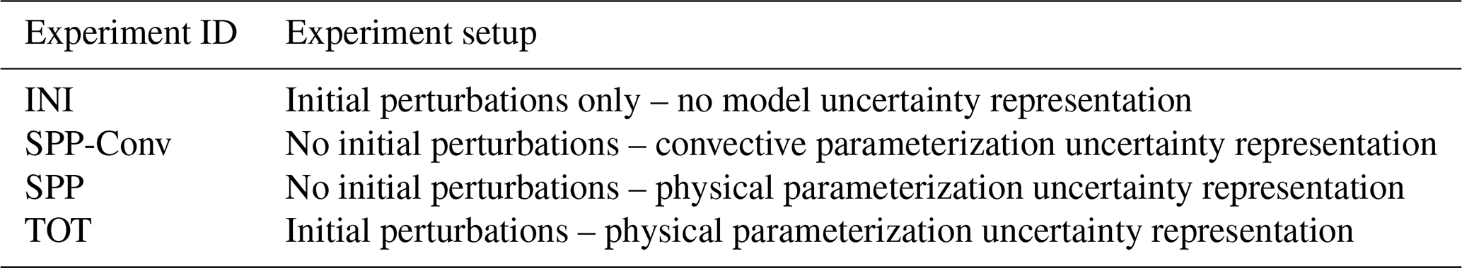
Table 1 Description of the different ensemble forecast experiments.

The ensemble forecast is coupled to the ECMWF wave model (ecWAM: ECMWF, 2021c) and to the Nucleus for European Modelling of the Ocean (NEMO) ocean model (Mogensen et al., 2012). The ecWAM provides the atmospheric model with the Charnock parameter, thus controlling the sea surface fluxes via the surface roughness. The atmospheric oceanic surface heat and moisture fluxes are controlled by the SSTs computed from NEMO every 20 minutes using a 0.25^∘ horizontal grid with 75 vertical levels. Due to the limited horizontal resolution of NEMO, the IFS is forced in the middle latitudes only, with fixed SSTs from the Operational Sea Surface Temperature and Sea Ice Analysis (OSTIA) product (Donlon et al., 2012) up to day 4, whereas beyond day 4 the SSTs from NEMO are used. The different types of experiments that have been carried out are reported in Table 1.

The first experiment is the ensemble forecast with initial-condition perturbation only (INI experiment). This is done by adding perturbation to a 4D-Var (Rabier et al., 2000) analysis. The perturbations are constructed from an ensemble of 4D-Var data assimilations (Buizza et al., 2008) where the size of the initial perturbations stems from the analysis uncertainty due to observation errors and model uncertainties including SPPT in the trajectory of the variational data assimilation. The second and third sets of experiments are conducted by running the ensemble with SPP applied. In the former (SPP-Conv) only the convective parameterization parameters are perturbed. In the latter (SPP) the convective, radiative, clouds and large-scale precipitation, turbulence, diffusion, and sub-grid orography parameterization parameters of the IFS model are perturbed, as briefly discussed below. In the last experiment (TOT) the operational forecast conditions of ECMWF are tested by including both the initial-condition perturbation and the physical parameterization perturbations.

2.2 Stochastically perturbed parameterizations ensemble

The stochastically perturbed parameterizations scheme represents model uncertainty in numerical weather prediction by introducing stochastic perturbations into the physical parameterization schemes (Lang et al., 2021) as mentioned above. The SPP is a new scheme aimed at replacing the currently used stochastically perturbed parameterization tendency (SPPT) scheme (Palmer et al., 2009) in the ECMWF ensemble forecast in June 2023. The new scheme, developed by Ollinaho et al. (2017), following the work of Baker et al. (2014) and Christensen et al. (2015), is based on applying perturbations directly to a selected number of parameters and/or equations within the parameterization schemes, usually those known to be specific sources of uncertainty for the model. The perturbations follow horizontal patterns that evolve stochastically in space and time. Each perturbed parameter is assigned an individual random field and different random fields are statistically independent. The log-normal distribution has been chosen for practical reasons as it ensures that the perturbed parameter values retain their original sign. The implementation of SPP allows the simultaneous perturbation of up to 27 parameters and variables in the deterministic IFS parametrizations of turbulent diffusion (Köhler et al., 2011), sub-grid orography (Beljaars et al., 2004), convection (Tiedtke, 1989; Bechtold et al., 2008), cloud processes and large-scale precipitation (Tiedtke, 1993; Forbes et al., 2011), and radiation (ecRad; Hogan and Bozzo, 2018). These 27 parameters and variables are reported in Tables S1–S4 in the Supplement, together with a detailed explanation of the choices behind their perturbation. As mentioned above, the SPP perturbation is applied through a 2D random field generator. In its implementation, SPP uses a single scale with a decorrelation length scale of 1000 km and a decorrelation time of 3 d (see Fig. 1 of Lang et al., 2021).

2.3 Validation data

In order to analyse the predictive skill of the ensemble, besides the operational analysis, the ensemble forecast perturbation experiments have been compared with the satellite-based, globally gridded global precipitation measurement (GPM) integrated multi-satellite retrievals for GPM (IMERG) (Huffman et al., 2020). In GPM-IMERG, the retrievals from geostationary satellites are blended seamlessly with information from the passive microwave (PMW) sensors from low-orbit satellites. This is done in order to achieve both a high accuracy and a high temporal (30 min) and spatial (≃ 10 km) resolution since the precipitation estimation based on the PMW alone suffers from a low sampling rate. Furthermore, the data are also calibrated by using rain gauges at the ground level. In this research, the 24 h accumulated precipitation values are used. The latter data are provided at the same resolution, 0.1^∘, as in the ensemble simulation.

2.4 Cyclone tracking

The method described here has been used to evaluate the tracks for both operational analyses, used as verification and ensemble forecasts. The tracking method is based on Picornell et al. (2014) and Ragone et al. (2018). The algorithm first aims at finding the local minima of the sea level pressure field at each time step. Then, for each minimum, the sea level pressure gradient of the sea level pressure along eight main directions (E, NE, N, NW, W, SW, S, SE) within a circle of radius 200 km is computed. The computed gradient is then chosen to be lower than 5 hPa per 200 km in at least six directions. After the minimum detection and filtering via selection through sea level pressure gradient, a proximity condition is applied to construct the complete trajectory. Starting from the first time step, each minimum is connected to the following one, at the following time step, that satisfies the condition of being closer than Δx=VΔt, with V=50 km h⁻¹ and Δt=3 h. If this condition is met, the two consecutive minima are considered to belong to the same trajectory. This condition was considered suitable and chosen according to the results of Ragone et al. (2018). Once the trajectories have been found, only the trajectories that last longer than 24 h and those that spend more than 12 h over the sea are selected. Trajectories that spend less than half their time over land or within 100 km of the coast are discarded.

2.5 Hart parameters

To analyse the three storms, the thermal structure and the thermal asymmetry have been investigated. The chosen parameter to quantify the latter has been recognized in the upper-level thermal wind, $-V_{\mathrm{T}}^{\mathrm{U}}$, which is considered to be a relevant parameter in distinguishing tropical-like cyclones from fully baroclinic cyclones (Mazza et al., 2017), and also in the thermal asymmetry, B. These parameters belong to the 3D cyclone phase space diagnostic introduced by Hart (2003). There, the thermal asymmetry is defined as the storm-motion-relative 900–600 hPa thickness asymmetry across the cyclone within its radius:

$$\begin{array}{}\text{(1)}& B=\left(\stackrel{\mathrm{‾}}{Z_{\mathrm{600}\mathrm{hPa}}-Z_{\mathrm{900}\mathrm{hPa}}}{|}_{\mathrm{R}}-\stackrel{\mathrm{‾}}{Z_{\mathrm{600}\mathrm{hPa}}-Z_{\mathrm{900}\mathrm{hPa}}}{|}_{\mathrm{L}}\right),\end{array}$$

where Z is the geopotential height, R indicates the right of current storm motion, L indicates the left of storm motion, and the overbar indicates the areal mean over a semicircle around the cyclone centre.

Instead, the cyclone's upper-level thermal structure (i.e. its cold or warm core) is indicated by $-V_{\mathrm{T}}^{\mathrm{U}}$. If it attains a positive sign, the cyclone attains an upper-level warm core. Indeed, the $-V_{\mathrm{T}}^{\mathrm{U}}$ is defined as

$$\begin{array}{}\text{(2)}& -\left|V_{\mathrm{T}}^{\mathrm{U}}\right|={{\displaystyle \frac{\partial \left(\mathrm{\Delta }Z\right)}{\partial \ln \left(p\right)}}}_{\mathrm{600}\mathrm{hPa}}^{\mathrm{300}\mathrm{hPa}}.\end{array}$$

The two pressure levels have been changed from 600 to 700 hPa and from 300 to 400 hPa due to the lower height of the tropopause in the mid-latitudes with respect to the tropics (Picornell et al., 2014). These values are computed within a 200 km radius around the detected cyclone centre by using the geopotential height field. In the Hart (2003) formulation, this radius was chosen to be 500 km, but given the smaller size of medicanes compared with tropical cyclones (Miglietta et al., 2013), the radius used in this study is smaller, 200 km. Since a positive value of lower-level thermal wind, $-V_{\mathrm{T}}^{\mathrm{L}}$, can characterize not only medicanes but also extratropical cyclones with warm seclusion (Hart, 2003), we consider important only the upper-level thermal wind, $-V_{\mathrm{T}}^{\mathrm{U}}$. In the case of the thermal asymmetry, the threshold value of B=10 m has been determined by analysing ECMWF reanalyses ERA40 at 1.125^∘ of the resolution, from which no major hurricane (winds of greater than 210 km h⁻¹) had associated with it a value of B that exceeded 10 m (Hart and Evans, 2001). Even if the threshold value of B has been originally determined for larger tropical/extratropical cyclones, previous studies have shown that such value is also useful in the case of medicanes (Miglietta et al., 2011). The deep warm core phase is represented by the asymmetry B being lower than 10 and closer to 0 and by a highly positive value of $-V_{\mathrm{T}}^{\mathrm{U}}$.

3 Overview of the storms

Table 2 provides a summary of the main features as retrieved by the analysis data: the storm duration, period, region of occurrence, asymmetry B, and upper-level thermal wind $-V_{\mathrm{T}}^{\mathrm{U}}$. The latter two parameters have been used for the computation of the cyclone phase space diagrams. The intensity (central pressure) and trajectory of each storm are shown in Fig. 1 along with the ensemble track.

Table 2 Duration, region of occurrence, central pressure (CP), thermal asymmetry parameter (B), and upper-level thermal wind ($-V_{\mathrm{T}}^{\mathrm{U}}$) from the operational analysis for each storm. The upper-level thermal wind and the thermal asymmetry parameter represent the parameters from the cyclone phase space of Hart (2003).

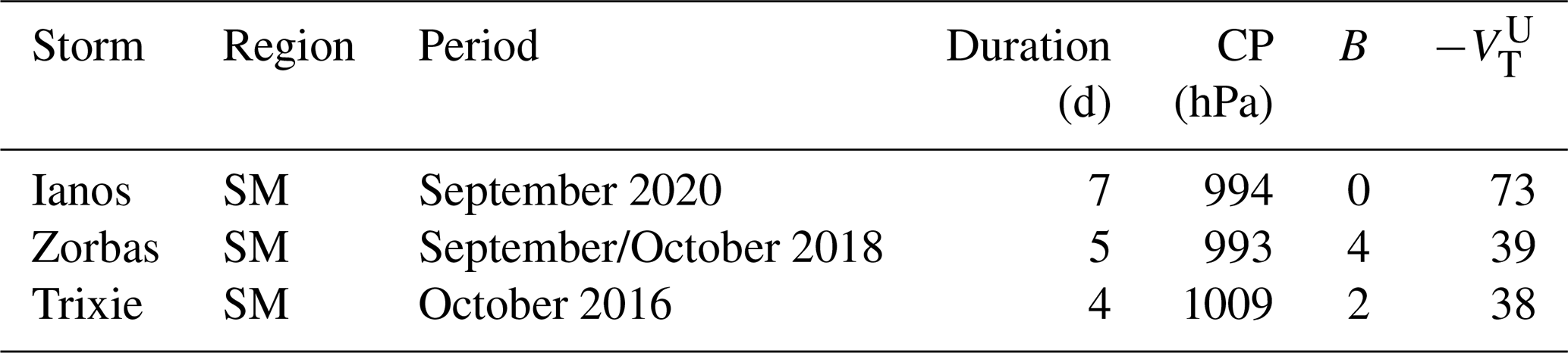
SM: southern Mediterranean.

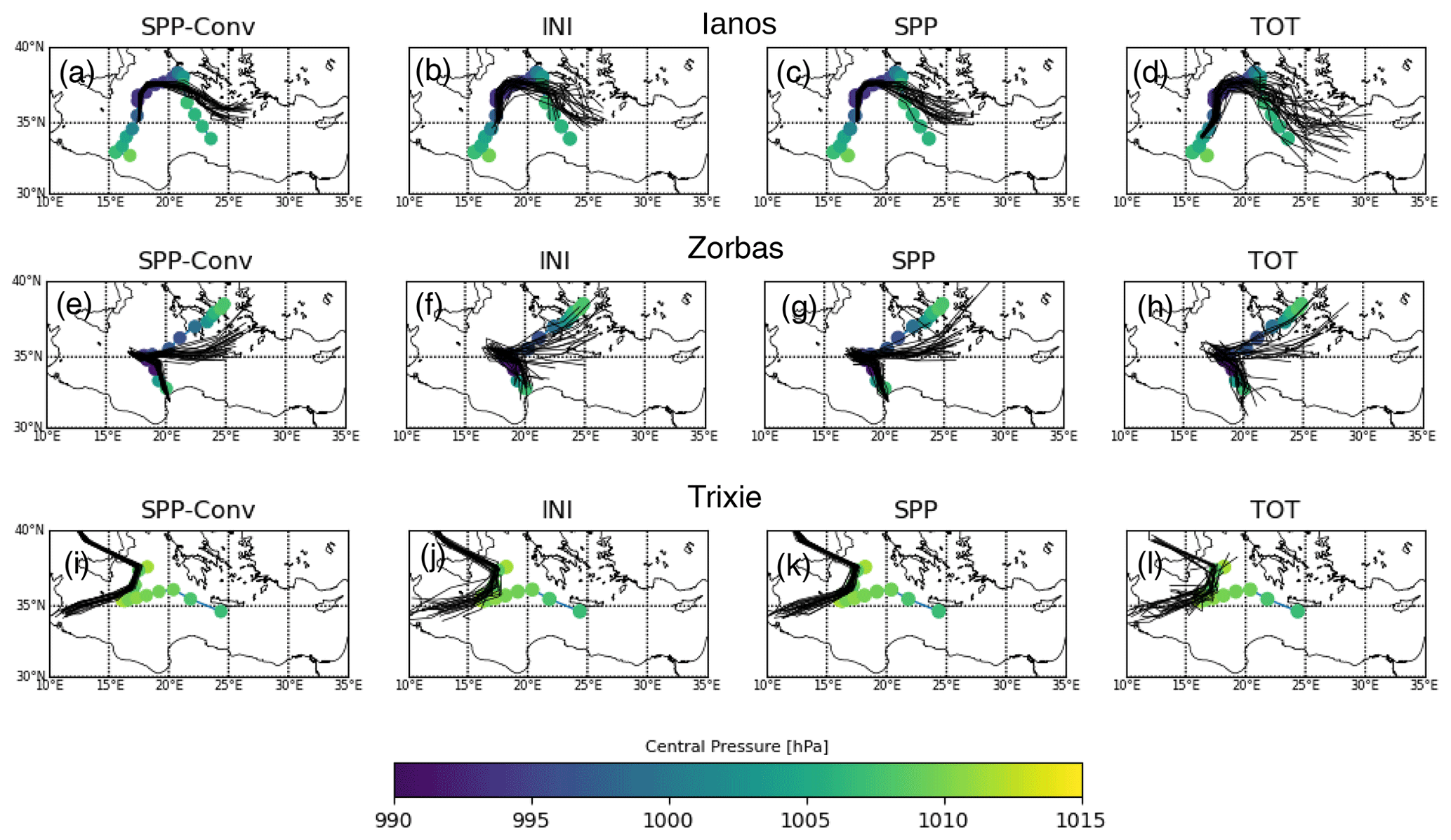
Figure 1 Track of the three storms for the operational analysis as reference track and for the ensemble members belonging to each experiment (SPP-Conv, INI, SPP, and TOT) for the three storms: Ianos (a)–(d), Zorbas (e)–(h), and Trixie (i)–(l). As background the operational analysis is reported with the colour representing the intensity, meaning the central pressure in hPa. For Ianos the experiments starting on 16 September have been chosen, for Zorbas the ones starting on 27 September, and for Trixie the ones starting on 27 October.

The three storms formed and developed in the same area, the southern Mediterranean, in the Ionian and Aegean seas. This region has one of the highest medicane occurrences as recognized in the literature (Cavicchia et al., 2014; Zhang et al., 2021). They occurred in the same period of the year, between September and November, the most frequent period for medicane occurrence (Romero and Emanuel, 2013). From Fig. 1 it can be gathered that there are some differences in duration and intensity, with Trixie being the longest-lasting of the three medicanes (in terms of the deepening phase) and Zorbas and Ianos being deeper than Trixie, as mentioned in the Introduction. As the track suggests (Fig. 1a), Ianos originated in the Gulf of Sidra. Then, between 14 and 15 September 2020, it emerged in the Gulf of Sidra and spent most of its life over the Mediterranean Sea, eventually reaching Greece on 17 September​​​​​​​ and turning southeastward, dissipating around 21 September. The analysis is capable of reproducing a value similar to the observed pressure minimum of 995 hPa (Comellas Prat et al., 2021).

Zorbas formed on 27 September 2018 close to North Africa and then moved into the central Mediterranean, turning eastward and moving over Greece into the Aegean Sea, where it finally decayed 4 d after its formation (Fig. 1d). Zorbas reached its maximum intensity (observed 992 hPa), which is well captured by the analysis.

Medicane Trixie formed on 28 October 2016. On 29 October it moved to the east of Malta, then on 30 October it moved eastward towards Greece (Fig. 1g) while dissipating. In the analysis, there was only a short intensification period evident, and the minimum pressure was fluctuating between 1010 and 1014 hPa during the period between 29 and 30 October, which might have been highly underestimated.

4 Results: ensemble forecast evaluation

This section examines the ensemble forecast experiments for certain aspects that are crucial for cyclones. The focus is put on cyclone track, cyclone intensity, as measured by central pressure (this value is considered the most stable and robust metric for assessing the intensity of a cyclone on a global scale (Davis, 2018)), as well as cyclone precipitation and thermal structure. The chosen parameters to quantify the latter are the above-mentioned upper-level thermal wind, $-V_{\mathrm{T}}^{\mathrm{U}}$, and thermal asymmetry, B. Finally, the tropical-like phase of these cyclones is thoroughly investigated.

4.1 Tracking

The ensemble tracking results are reported in Fig. 1. As examples, the tracks starting on 16 September are shown for Ianos, the ones starting on 27 September are shown for Zorbas, and the ones starting on 27 October are shown for Trixie.

By looking at Fig. 1a–d and e–h the ensemble tracks follow the references for Ianos and Zorbas respectively. On the contrary, for Trixie, the tracking, which starts 1 d prior to the starting date of the reference track (starting on 28 October), follows the track until the early hours of 29 October (Fig. 1i–l) when it diverges and ends up in North Africa, underlying a missed forecast. This is consistent also for earlier starting dates (25 and 26 October) with a greater error in terms of initial position (not shown). Figure 1 shows that, as expected, the simulations with initial-conditions perturbations (INI and TOT) tend to show more spread in the initial position. However, the spread at later stages in the simulation seems to be similar for both the INI experiment and the two experiments with the physics perturbation, SPP and SPP-Conv, while on the other hand, the TOT experiment shows a slightly higher spread than the other simulations.

For Ianos 16 September was chosen as an example, but the behaviour for the three starting dates is quite similar, with the trajectory being reproduced quite well for the first days and the error increasing with time. The error is calculated as the root mean square error between the ensemble mean track and the reference track. It never exceeds 300 km (not shown) and is always below 100 km up to 48 h (not shown). The error values are similar in all four experiments but slightly lower for the INI and TOT experiments. In the case of Zorbas and Trixie, since the starting dates are earlier than the start of the reference track, the earlier the simulations start, the greater the uncertainty in the start position, and hence the greater the spread. Figure 1 shows the latest simulated starting dates for all cyclones. For Zorbas, starting on 27 September, the obtained tracks follow the reference with a small error, at least for the first days, which is anyway always below 300 km in later stages. As in the case of Ianos, the error made by the four experiments is similar. For Trixie, the error goes up to 700/800 km for the four experiments with respect to 27 October, the last start date shown in Fig. 1g–i.

The tracking results shown in Fig. 1 are mirrored by the ensemble spread and the relationship between the spread and the error presented in Figs. 2 and 3 respectively. Following the approach of Hamill et al. (2011), the spread of the ensemble for a single cyclone ensemble forecast at a given forecast time is defined as

$$\begin{array}{}\text{(3)}& S_l\left(t\right)={\displaystyle \frac{\mathrm{1}}{n}}\sum _{i=\mathrm{1}}^n{D}_i,\end{array}$$

where D_i denotes the great-circle distance of the ith ensemble member position of the cyclone from the ensemble mean cyclone position. The total number of ensemble members used for the calculation is 24 and the spread has been computed for each starting date (three dates for each medicane). The results, reported in Fig. 2, are for the same start date as in Fig. 1, i.e. 16 September for Ianos, 27 September for Zorbas, and 27 October for Trixie, which is also representative of the spread of the other start dates. It is found that the TOT experiment has the largest mean track spread for the three cyclones (Fig. 2a, b, and c) but is comparable to the INI ensemble for most of the simulation period. The spread for the SPP and SPP-Conv ensembles is comparable and lower than the other two experiments but reaches a similar value to the INI ensemble at the end of the simulation. Ianos and Zorbas show less spread than Trixie at initialization, especially for the INI and TOT experiments (which are probably dominated by the initial perturbation at the beginning). This may be due to the fact that for Trixie, whose analysis track starts on 28 October (Fig. 1g to i), there is a large uncertainty in the initial position. Looking at the spread/skill relationship (Fig. 3), measured by the ratio of the ensemble spread and the root mean square error between the ensemble mean track and the reference track, it can be said that as mentioned before the error is always larger of the ensemble spread, and the spread and the skill are only comparable in the first hours of the simulations (20–40 h) when the spread/skill values are closer to one. The SPP, the SPP-Conv, and the INI are generally more under-dispersed than the TOT experiment in all three cases. The former three experiments behave generally in the same way, with the INI experiment showing less error after the second day for Ianos and Zorbas but behaving similarly for Trixie. The TOT experiment performs better for Zorbas but not for Trixie and Ianos.

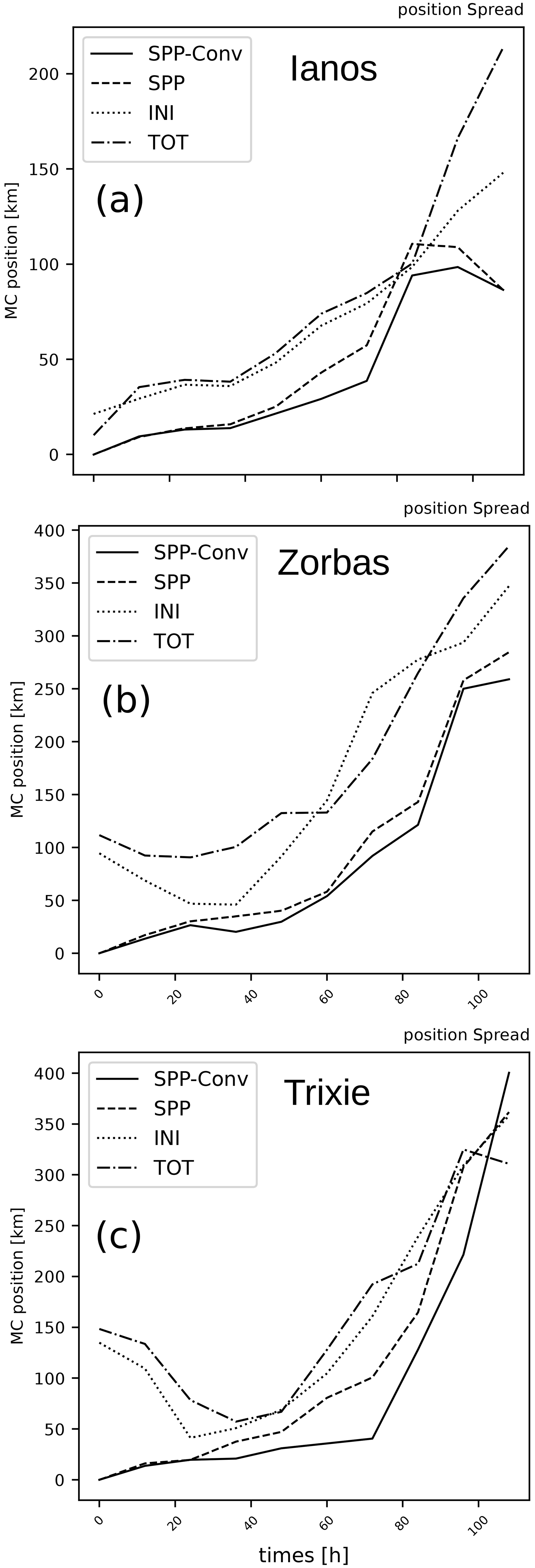
Figure 2 Mean ensemble spread of the medicanes track for each ensemble perturbation experiment for Ianos (a), Zorbas (b), and Trixie (c). The track spread is computed as described in Eq. (3) and is reported in kilometres. For Ianos the experiments starting on 16 September have been chosen, for Zorbas the ones starting on 27 September, and for Trixie the ones starting on 27 October, in order to be consistent with the ensemble tracks shown in Fig. 1.

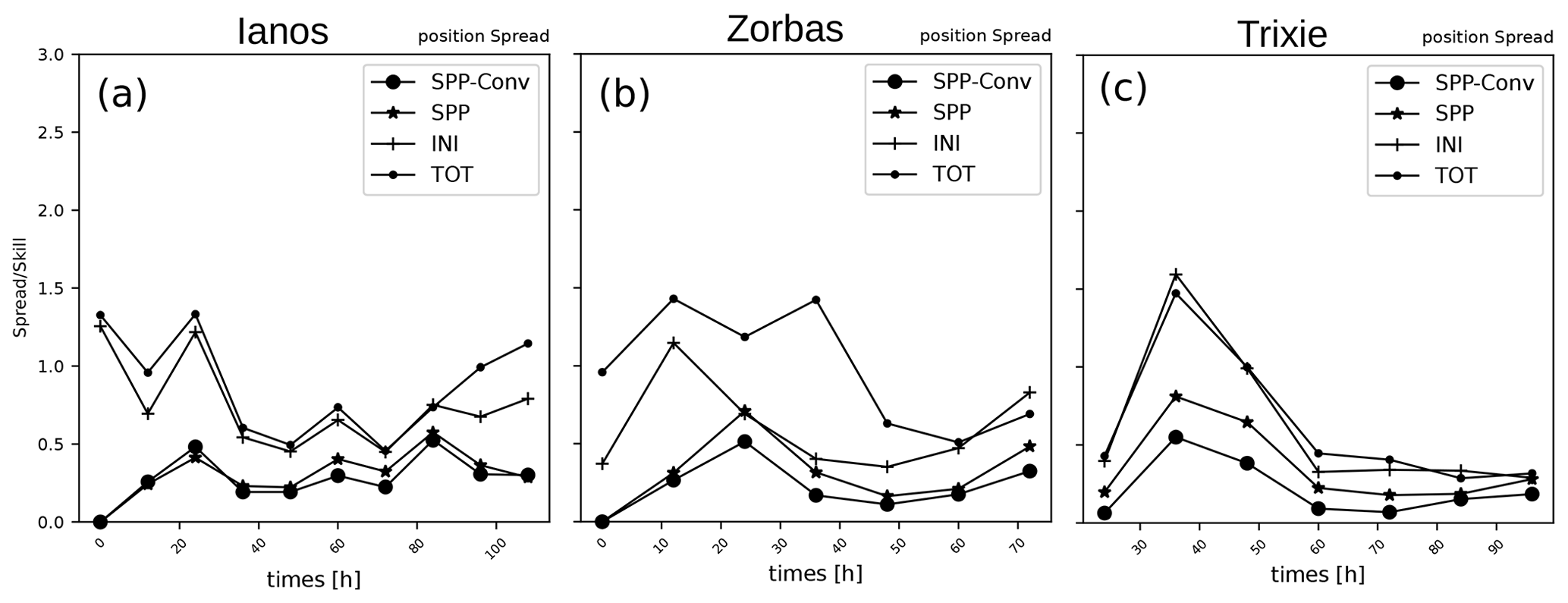
Figure 3 Ensemble spread/skill relationship for each ensemble perturbation experiment for Ianos (a), Zorbas (b), and Trixie (c). The spread is computed as in Eq. (3) and the skill is the root mean squared error between the ensemble mean and the analysis tracks. For Ianos the experiments starting on 16 September have been chosen, for Zorbas the ones starting on 27 September, and for Trixie the ones starting on 27 October, in order to be consistent with the ensemble tracks shown in Fig. 1.

At later forecast steps, Trixie is the cyclone with the highest spread for all three perturbations compared with Ianos and Zorbas. By looking at the general spread trends, while during the first 2 d of the simulations the initial perturbations dominate the spread for all cases, by day 3 the spread from the physical parameterizations becomes equivalent. As a result the spread of the TOT ensemble, which is a combination of the two, tends to compare well with the INI ensemble at the beginning of the simulation and then to the SPP and SPP-Conv at later stages. The INI experiment spread is highest at initialization, as also seen in Lang et al. (2012), since the EDA perturbations are associated with a shift and intensification or weakening of the cyclone. Even considering the case-to-case variability, in terms of the spread of the track, the SPP-Conv experiment is the one with consistently less spread for all the cyclones. The low error values obtained by Ianos and Zorbas, compared with those obtained in the case of Trixie (≥ 800 km), make it not only the medicane with the largest spread but also the one with the most significant error. Indeed, it has been verified that this particular simulated cyclone deviates from the analysis track. The simulation track of Trixie is probably due to the fact that the ensemble forecast does not correctly capture the processes associated with cyclogenesis, but it can also be related to the fact that the simulations start too early before the appearance of the medicane. This is an aspect also recognized by Di Muzio et al. (2019) in the simulation of these events.

Interestingly, both SPP experiments, and specifically the SPP-Conv, produce cyclone spread that is comparable at the later stages of the simulation to the experiment with initial-condition perturbations only. Similar results have been found in Lang et al. (2012), underlining the initial-condition and physical heating-related sources of uncertainty in the tracking of these cyclones.

4.2 Intensity

The other important aspect investigated is the intensity of the cyclones analysed. The intensity is assessed by studying the minimum core pressure at the cyclone position.

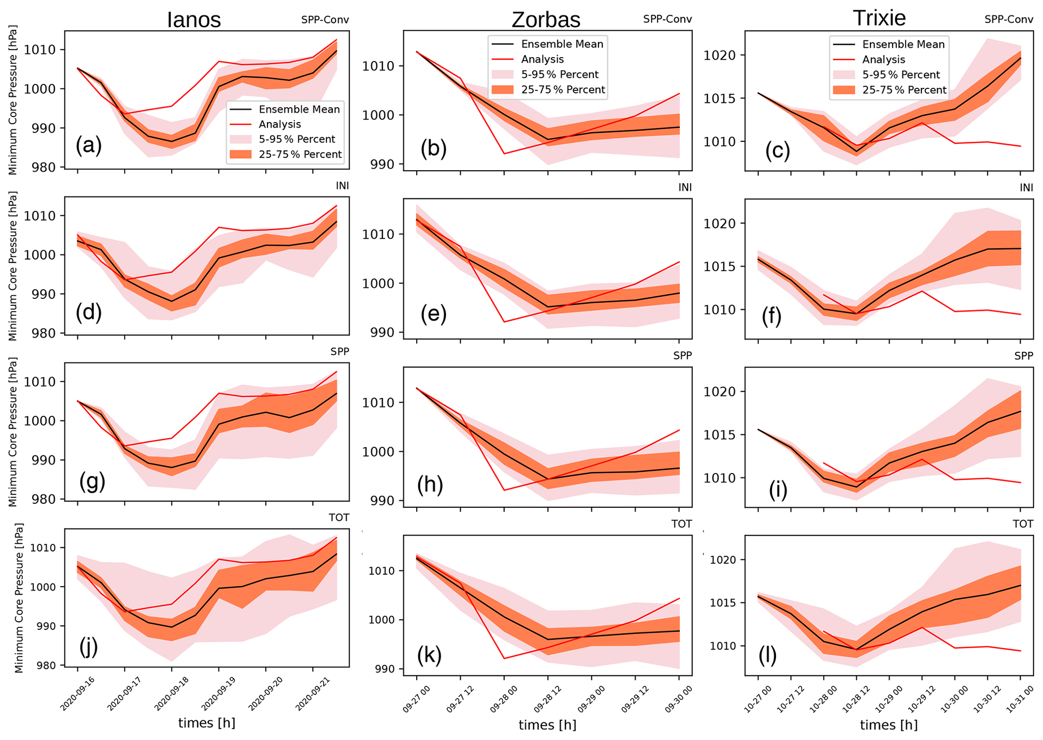
Figure 4 Analysis of the mean seal level central pressure for Ianos, Zorbas, and Trixie. The plots show the ensemble members' development throughout the simulation. In each panel the ensemble mean is reported in black, the operational analysis is reported in red, and the two shaded areas represent the 25 %–75 % percentile and the 9 %–95 % percentile. The SPP-Conv experiment is reported for each medicane in (a)–(c). The INI experiment is reported in (d)–(f), the SPP experiment in (g)–(i), and the TOT experiment in (j)–(l).​​​​​​​

The development of the core pressure with the simulations is reported in Fig. 4 where the mean sea level pressure at the centre of the cyclone (minimum core pressure in Fig. 4) is shown, with the ensemble mean, the 25 %–75 % percentile, and the 5 %–95 % percentile compared with the analysis values for the four ensemble experiments for the chosen starting dates as an example. For Ianos there is an overestimation of the cyclone deepening (Fig. 4a, d, g, and j), with a time shift of 1 d, compared with the analysis value, which is consistent in all four experiments. For Zorbas the minimum pressure is underestimated only in the case of the SPP-Conv experiment; however, there is a shift of 12 h compared with the analysis time shift in the four experiments (Fig. 4b, e, h, and k). In the case of Trixie, there is an underestimation (Fig. 4c, f, i, and l) and the ensemble experiments are not able to capture the full evolution of the cyclone pressure (especially the second deepening around 30 October).

For all three cyclones, the spread is slightly higher for the SPP and the SPP-Conv experiments compared with the INI one; however, the TOT experiment is the one with the highest spread for the three cyclones. The reference analysis is included in the ensemble spread of the latter experiments (INI and TOT) compared with what happens with the SPP experiments, at least in the initial time steps. This is particularly true for Ianos (Fig. 4a, d, g and j). For Zorbas, the pressure deepening is slightly better captured by the SPP and the TOT ensembles (Fig. 4b, h and k). As pointed out before, there is a shift in the minimum pressure of 12–24 h compared with the analysis value. For Ianos this is also present in the simulation starting on 15 September but is absent in the simulation starting on 17 September. This is due to the improved initial conditions when the forecast starts closer to the event. The same can be said for Zorbas. For Trixie, apart from the first deepening happening on 28 October, which is well captured by all the experiments, the second minimum, which is the deepest, is not captured by any of the experiments' ensemble members, even when starting on 27 October (the last start date). In general, there is an underestimation of the minimum core pressure, and its evolution up to 29 October is captured better by the TOT experiment, followed by the SPP experiment (Fig. 4i and l). Overall, the TOT ensemble, the operational forecast at ECMWF, performs better in terms of core pressure, since it includes both the initial perturbation and the model perturbation.

4.3 Precipitation

The precipitation field has also been analysed and verified against observation. The verification field is chosen to be the precipitation, as in Vich et al. (2011) and Montani et al. (2011). Matching the forecast with the verifying data is hampered by the irregularly spaced ground network of observations and by the spatial variability of precipitation. Therefore, satellite products, in particular the above-mentioned integrated multi-satellite retrievals for GPM (GPM-IMERG), are used.

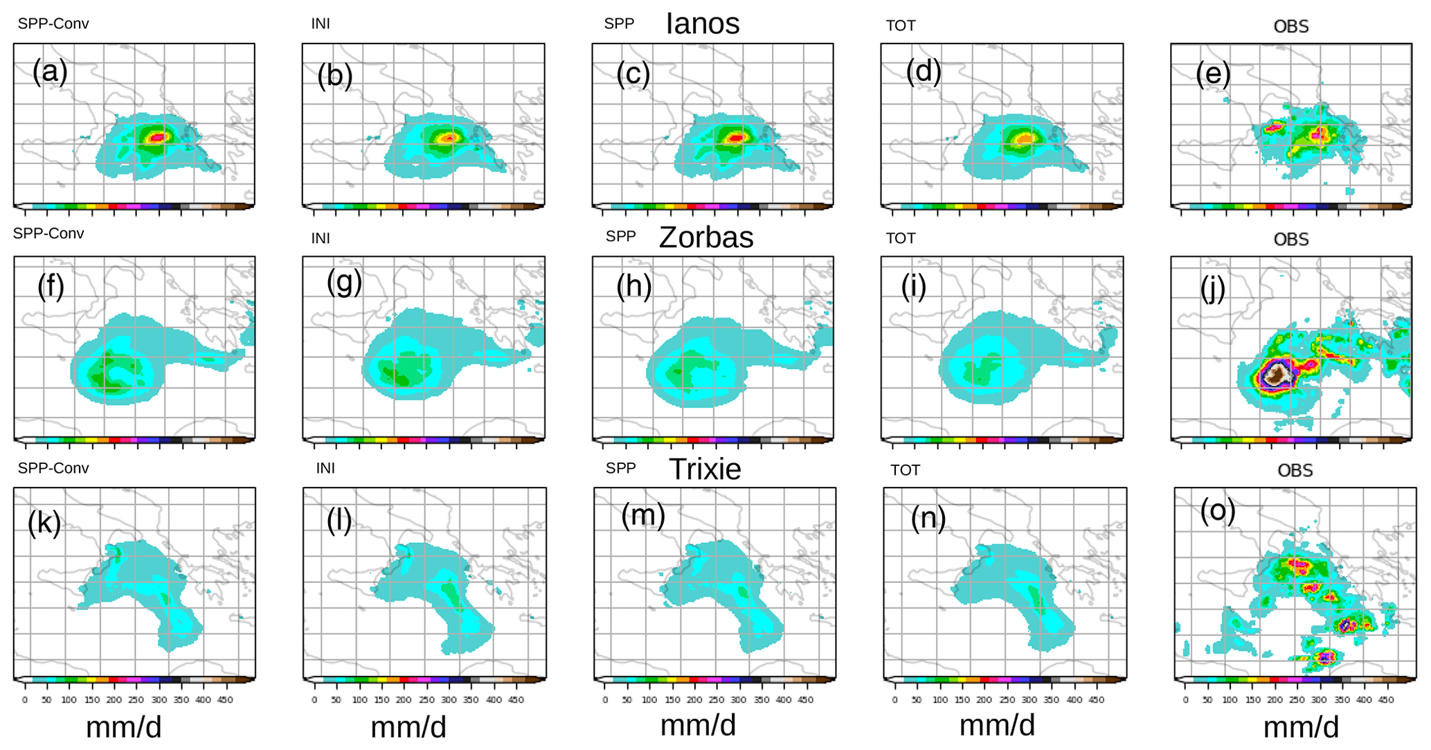
Figure 5 Daily accumulated precipitation (mm d⁻¹) for the three ensemble experiments' ensemble means compared with the satellite observation GPM-IMERG. For Ianos 17 September is shown in (a)–(e). For Zorbas 28 September is shown in (f)–(j). For Trixie 28 October is shown in (k)–(o). The SPP-Conv ensemble forecast accumulated precipitation is reported in the first column, the INI ensemble in the second column, the SPP ensemble in the third column, the TOT ensemble in the fourth column, and the observations in the fifth column.

The precipitation structure of the three medicanes, in terms of intensity and position, is similar to what is observed in tropical cyclones (Zhang et al., 2021, 2019). Indeed, there are similarities in their rainfall structures and those for Mediterranean cyclones (Flaounas et al., 2018) where most precipitation associated with medicanes is concentrated to the northeast side of the cyclone centre, as is shown in Fig. 5 for the three cyclones. For the three cyclones, the ensemble mean of the last starting date is shown. For each cyclone, the daily accumulation on the day of the “tropical-like” phase is shown in Fig. 5. For Ianos this is 17 September, for Zorbas 28 September, and for Trixie 28 October. The daily accumulation values from the ensemble forecast experiments are comparable to the observed values only regarding Ianos. In general, the maximum is better captured by the SPP experiments for Ianos (Fig. 5a and c), while for Zorbas and Trixie this is true for the INI, the TOT and the SPP-Conv experiments (Fig. 5f, g, and i). The standard deviation of each ensemble experiment shows that there is higher uncertainty associated with the higher values of the precipitation distribution (Fig. S1 in the Supplement). This is consistent for all three cyclones. There is little difference between the SPP-Conv and the SPP experiment in terms of precipitation distribution. This mirrors what is shown in Fig. 4.

The positioning of the maximum precipitation in the presented distributions (Fig. 5) is generally consistent with the observed GPM-IMERG distribution. However, for all three cyclones, there are some other secondary maximums in the distribution that are not well captured. This is possibly related to the simulation resolution not being able to capture completely the precipitation structure. Preliminary results from the recent work of the Destination Earth (DestinE) project (Gascón et al., 2023) shows that the accumulated precipitation pattern is slightly better captured by the 4 km simulation compared with the 9 km one with the IFS model (https://confluence.ecmwf.int/display/DES/ME2b+-+Differences+47r3+vs+48r1, last access: 26 October 2023, for Ianos, reported as an example).

The daily accumulated precipitation shown in Fig. 5 belongs to the simulations with the latest starting date, where the maximum precipitation is better captured. Indeed, the error in the simulated ensemble mean precipitation maximum compared with the observation decreases with the forecast start date closer to the medicane occurrence. This is specifically true for Ianos and Zorbas (as shown in Fig. S2), while for Trixie the maximum is also underestimated. For Trixie, the simulation is not able to capture the intensity of the precipitation. This is linked to the absence of the deepening of the cyclone, and the precipitation starts to decrease in a significant way after 28 October. This is seen across the range of starting dates.

In the fourth column of Fig. 5, the TOT ensemble means are shown. The latter ensemble mean compares well to the INI ensemble, similar to what happens for the standard deviation of each ensemble experiment (Figs. S1 and S2), thus confirming the results of the tracking and intensity.

4.4 Thermal structure and asymmetry

The Hart parameters, $-V_{\mathrm{T}}^{\mathrm{U}}$ and B, are analysed in Fig. 6. We limit our physical analysis of the Hart parameters and the heating and intensification to the experiments with either initial or physical perturbations. The focus is on the values where the cyclone deepening occurred in the observation; thus, the values in Table 2 are reported as references in Fig. 6. The violin plots of the forecast distribution for each experiment at different starting dates are shown with the median (white dot) and the interquartile range (grey bar). The sections at the sides of each violin plot represent the kernel density estimation to show the shape of the distribution of the data. (The wider sections of the violin plot represent a higher probability that members of the population will take on the given value, and the thinner sections represent a lower probability.) The choice for the violin plot was made because, unlike a box plot that can only show summary statistics, violin plots depict summary statistics and the density of each variable. In Fig. 6 only the SPP-Conv and the INI experiments are shown for comparison, because the results of the SPP experiments, as already pointed out above, are very similar to those obtained by the SPP-Conv.

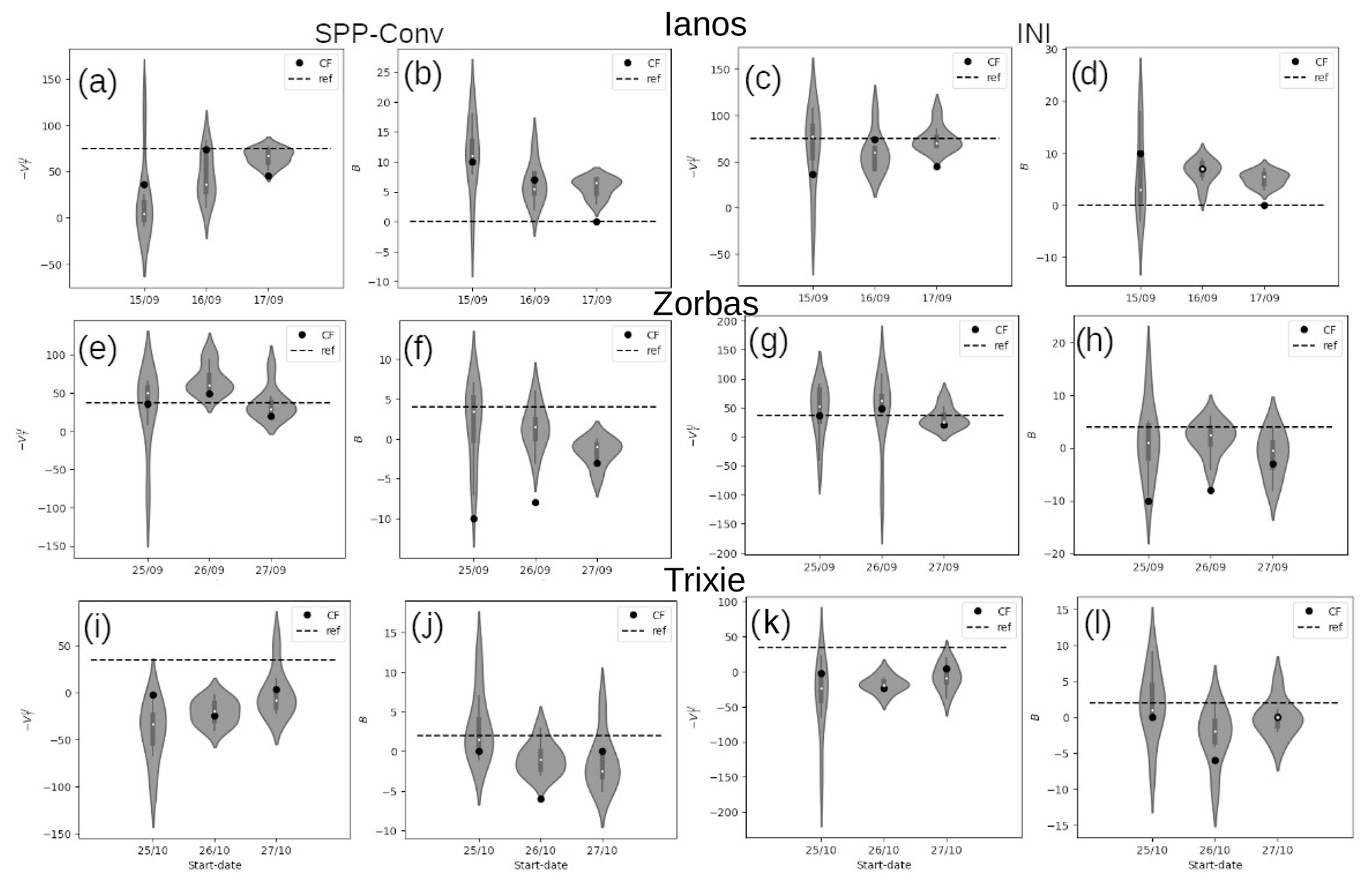
Figure 6 Ensemble forecast violin plots of thermal wind, $-V_{\mathrm{T}}^{\mathrm{U}}$, and thermal symmetry, B, for each starting date for Ianos in (a) and (b) for the SPP-Conv ensemble forecast and (c) and (d) for the INI ensemble forecast, for Zorbas in (e) and (f) for the SPP-Conv ensemble forecast and (g) and (h) for the INI ensemble forecast, and for Trixie in (i) and (l) for the SPP-Conv ensemble forecast and (m) and (n) for the INI ensemble forecast. The violin plot is a hybrid of a box plot and a kernel density plot, which shows peaks in the data. The white dot represents the median, the thick grey bar in the centre represents the interquartile range (25th–75th), and the thin grey line represents the rest of the distribution. On each side of the grey line is a kernel density estimation to show the distribution shape of the data.

The forecast distribution in the three ensemble experiments presents different behaviours compared with the analysis reference value (ref in Fig. 6) and the starting date in the three experiments. In general, the three ensemble experiments can reproduce the thermal structure of the storms, showing in some cases a reduced spread with the forecast start date closer to the occurrence, probably related to the fact that these starting dates coincide with the period in which the cyclone had already developed (see Fig. 6a and c for Ianos) and that the appearance of a symmetrical storm can benefit from improved initial conditions (Di Muzio et al., 2019). This behaviour is consistent for all three perturbation experiments.

The Ianos simulations show a reduced spread with later starting dates accompanied by the distribution value approaching the analysis value for the thermal wind (Fig. 6a and c) and the thermal asymmetry (Fig. 6b and d). In particular, for the thermal asymmetry B, this makes the spread of the ensemble to be included below the threshold of 10 m which would define the system as a frontal system rather than a non-frontal one (Miglietta et al., 2013), thus showing a better performance in reproducing the tropical-like phase of medicanes. This is true for both experiments, INI and SPP-Conv, as well as for Zorbas and Trixie. In the case of Zorbas, there is a usually smaller spread for the last starting date only regarding the thermal wind (Fig. 6e and g). Instead, there is a comparable spread for the thermal asymmetry, especially for the INI experiment (Fig. 6h). However, the forecast distribution of both experiments contains the reference analysis values for both the thermal wind and the thermal asymmetry (Fig. 6e to h). In Trixie, the spread is comparable between the starting dates for the thermal asymmetry parameter and thermal wind (Fig. 6i to l). There is a consistent underestimation of the thermal wind (with median values of $-V_{\mathrm{T}}^{\mathrm{U}}$ around −25 to −50) in all three ensemble experiments. The forecast distribution is closer to the analysis values ($-V_{\mathrm{T}}^{\mathrm{U}}=\mathrm{39}$) for the third starting date, for both ensemble experiments, as shown in Fig. 6i and k. This underestimation of the upper-level thermal wind means that a warm core was never reached in the ensemble forecast experiments, as will be explored in the following sections.

5 Results: physical processes analysis

To understand the processes of cyclone formation, intensification, and tropical-like phase, and how they affect the forecast, a comparison was made between the operational analysis and the ensembles. To reduce the amount of data, the analysis of the ensembles was reduced to consider a subset of 8 members instead of 24.

5.1 Cyclone formation

The synoptic environment favouring cyclogenesis in the Mediterranean is the presence of a deep upper tropospheric trough, cut off from the large-scale circulation and intruding into the Mediterranean. The latter can bring thermodynamic disequilibrium, owing to its deep cold air (Emanuel, 2005; Flaounas et al., 2022). As the low approaches the Mediterranean environment with small baroclinicity, the air masses are lifted, decreasing the temperature above and increasing convective instability. The presence of an intrusion of very cold air in the upper troposphere may allow for the conversion from thermal energy into kinetic energy (Palmen, 1948). This is usually accompanied by the presence of air masses with high potential vorticity (PV) intruding in the Mediterranean region (Flaounas et al., 2022), which usually triggers instability also in the case of extratropical cyclones (Flaounas et al., 2015; Raveh-Rubin and Flaounas, 2017). This stratospheric air mass can introduce anomalous high PV in the upper troposphere, which induces thermodynamic instability strengthening the surface vortex below. Usually, this stratospheric air mass intrusion is called PV streamer (Claud et al., 2010) and it is evidenced here that it is present in all three medicanes. This is underlined in Fig. 7a–c for the operational analysis in which the height of the isosurfaces of 2 PVU (PVU = 10⁻⁶ m² K kg⁻¹ s⁻¹) is shown in relation to the mean sea level pressure for the three medicanes. These factors have already been found to be an integral part of Ianos and Zorbas formation in the literature, while for Trixie, to the authors' knowledge, these aspects have never been fully analysed. For Ianos, on 16 September the cutoff low was present (clearly identified at the 500 hPa level in Fig. S3) and the PV streamer approached the area over the low centre and wrapped around it (not shown), as also evidenced in Lagouvardos et al. (2022). Then, on 17 September, as shown in Fig. 7a, the PV streamer broke up, resulting in the formation of a PV cutoff. Similarly, the formation of a PV streamer with the cutoff low already present (Fig. S3) on 27 September over the Mediterranean was followed by cyclogenesis of Zorbas at the PV southeastern flank (Portmann et al., 2020), as it is shown in Fig. 7b, followed by a PV cutoff (not shown for the analysis but reported in Fig. S6 for the ensemble experiments). For Trixie, the presence of a cutoff low on 28 October (Fig. S3) is accompanied by the PV streamer reaching the area in which the cyclone is forming, even if the interaction between the PV streamer and the cyclone is not so evident (Fig. 7c). However, it is noted here that the PV cutoff is never reached (reported in Fig. S6 for the ensemble experiments).

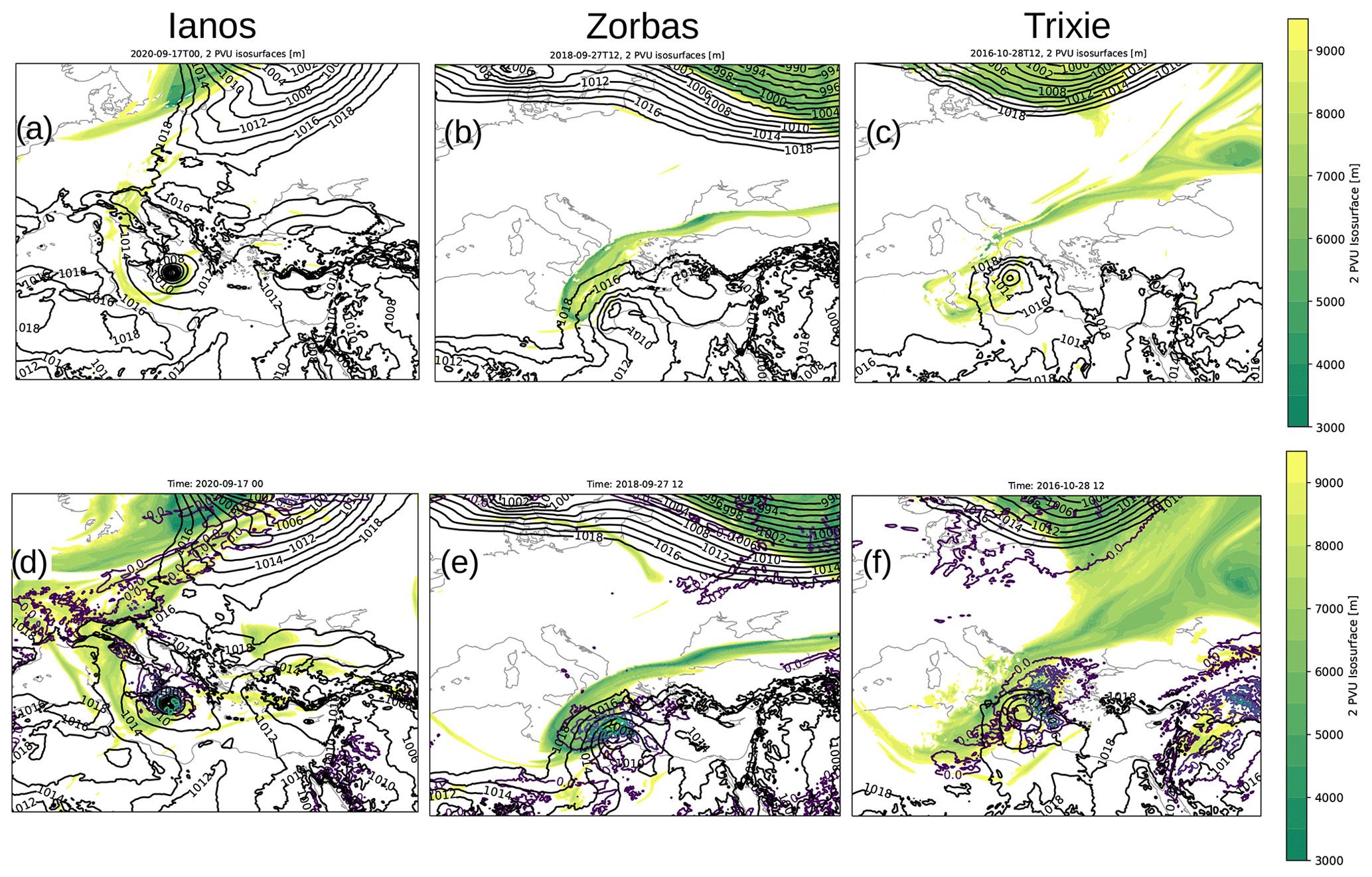
Figure 7 Height of the 2 PVU (PVU = 10⁻⁶ m² K kg⁻¹ s⁻¹​​​​​​​) isosurfaces together with the mean sea level pressure (black lines) in the operational analysis. For Ianos 17 September at 00:00 UTC is reported in (a) in the operational analysis and (d) for the SPP-Conv ensemble experiment ensemble mean, for Zorbas 27 September at 12:00 UTC is reported in (b) in the operational analysis and (e) for the SPP-Conv ensemble experiment ensemble mean, and for Trixie 28 October at 12:00 UTC is reported in (c) in the operational analysis and (f) for the SPP-Conv ensemble experiment ensemble mean. For Ianos (d) is from the ensemble starting on 17 September, for Zorbas (e) is from the ensemble starting on 26 September, and for Trixie (f) is from the ensemble starting on 26 October.

For Ianos in general, the PV streamer is well reproduced by the SPP-Conv and the other ensembles (not shown), especially regarding its interaction with the heating at 500 hPa (yellow to blue coloured lines in Fig. 7d). However, on 17 September at 00:00 UTC the PV streamer detachment from the large-scale has not happened yet, as Fig. 7d shows, but it will happen 12–24 h later (Fig. S6) which is in line with what is shown in Fig. 4 regarding the simulated minimum central pressure reaching the lowest value with a delay compared with the analysis value. This delay means that both in the analysis and the ensembles the medicane reaches its maximum intensity with the creation of the PV cutoff, meaning that the former is dictated by the latter, at least for the timing. If starting on 17 September, the three ensembles can reproduce the PV cutoff from the large scale at the right timing (not shown) probably due to initial conditions being closer to the tropical-like conditions. When looking at the ensemble performance, a more in-depth analysis is carried out using the divergence (s⁻¹), vorticity (s⁻¹), and time tendencies of the temperature (K s⁻¹) and specific humidity (g kg⁻¹ s⁻¹) profiles around the cyclone centre (within a radius of 200 km). The latter profiles are reported in Figs. 8–10 for the SPP-Conv experiment and in there the temperature and humidity tendency are reported as Q1 and Q2 for temperature and humidity respectively, as is usual in the literature (Grabowski et al., 1999; Yanai et al., 1973), where $Q\mathrm{1}=\frac{\mathrm{d}T}{\mathrm{d}t}$ and $Q\mathrm{2}=-\frac{L_v}{c_P}\frac{\mathrm{d}q}{\mathrm{d}t}$, with Q1 representing the heating in Fig. 7. In the case of Ianos, which becomes a warm core cyclone on 17 September (Fig. 8c and d at 00:00 UTC), the Q1 signals that the warming is happening at 500 hPa and it has deepened from 12 h earlier, on 16 September (Fig. 8a at 12:00 UTC), where the maximum is located at 600 hPa. For Zorbas, the PV streamer is evident and it is occurring 1 d prior to the tropical phase (Fig. 7b), thus inducing an intensification of the cyclone. This is well reproduced by the SPP-Conv ensemble experiment shown in Fig. 7e, as well as for the other two ensemble simulations INI and SPP (not shown). The values of the height of the 2 PVU isosurfaces coincide between the operational analysis (in Fig. 7a, b, and c) and the ensemble simulations (in Fig. 7d, e, and f). Similar behaviour to the one seen in Ianos, regarding the heating, can be observed for Zorbas in Fig. 9a and b. On 27 September at 12:00 UTC the heating is below 600 hPa even if there is already a weak divergence over 600, underlining the presence of a still shallow vortex. Once again the PV cut- off will happen 12 h later when Zorbas will also reach the maximum intensity as indicated by Fig. 4 where a similar delay of 12 h is present.

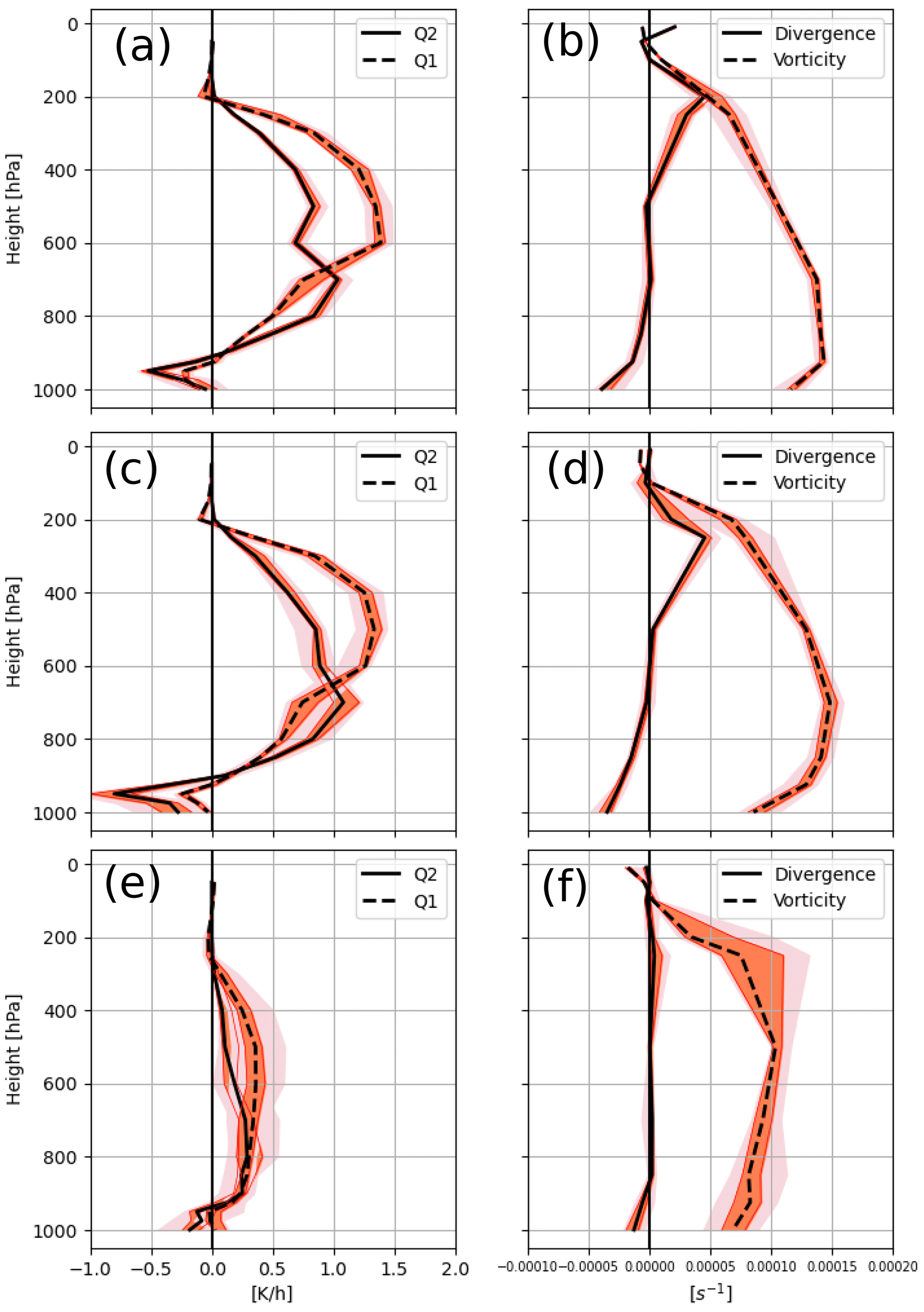
Figure 8 Analysis of the intensification and transition to tropical-like characteristics for Ianos as represented by the SPP-Conv experiment. The $Q\mathrm{1}=\frac{\mathrm{d}T}{\mathrm{d}t}$ and $Q\mathrm{2}=-\frac{L_v}{c_P}\frac{\mathrm{d}q}{\mathrm{d}t}$ profiles are shown in the first column and the vorticity and divergence profiles are shown in the second column. Panels (a) and (b) are from 16 September at 12:00 UTC. Panels (c) and (d) are from 17 September at 00:00 UTC. Panels (e) and (f) are from 20 September at 12:00 UTC. These profiles belong to the simulation starting on 16 September. The colour shading is the same as in Fig. 4.

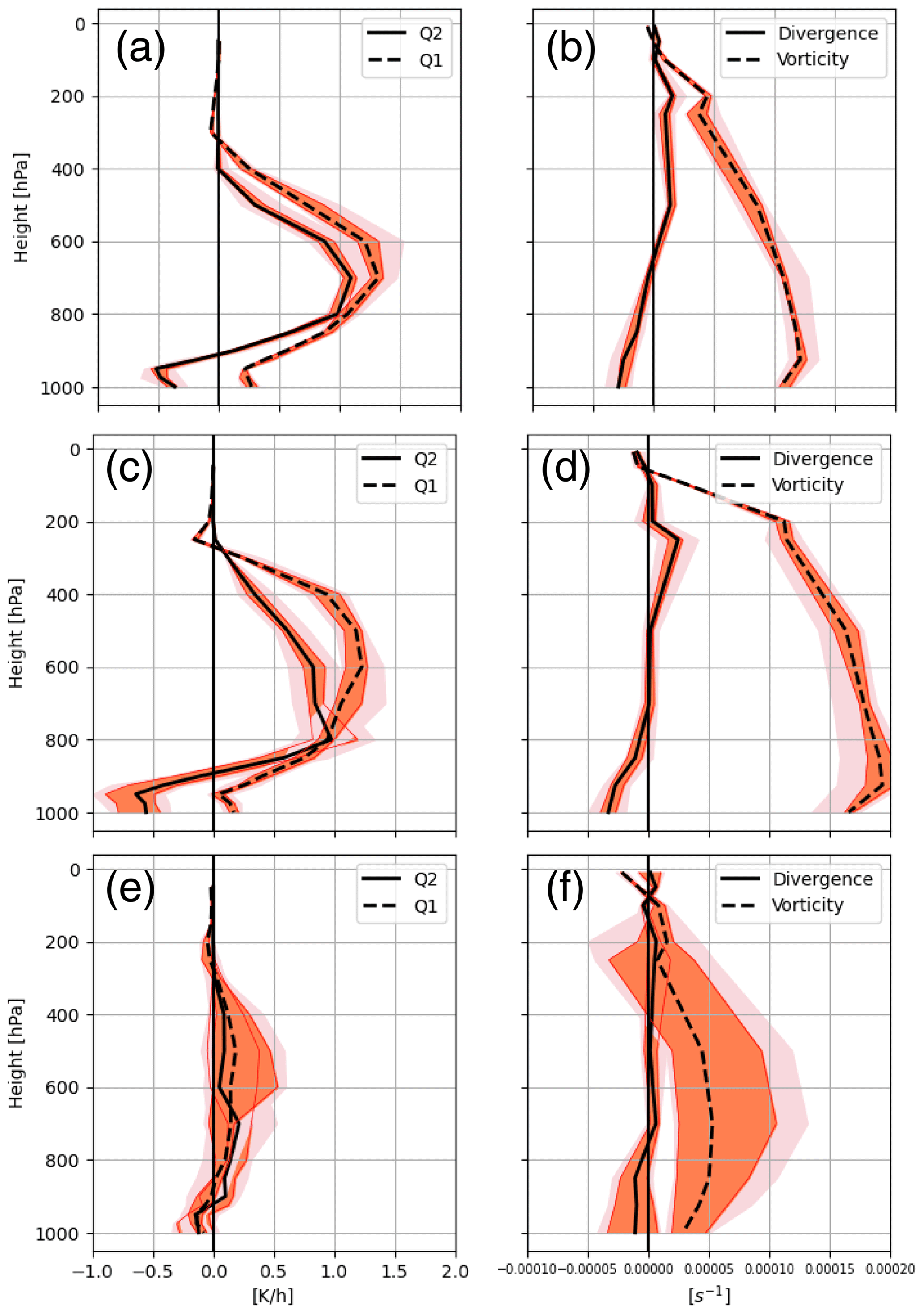
Figure 9 Same as Fig. 8 but for Zorbas. Panels (a) and (b) are from 27 September at 12:00 UTC. Panels (c) and (d) are from 28 September at 12:00 UTC. Panels (e) and (f) are from 1 October at 12:00 UTC. These profiles belong to the simulation starting on 27 September. The colour shading is the same as in Fig. 4.

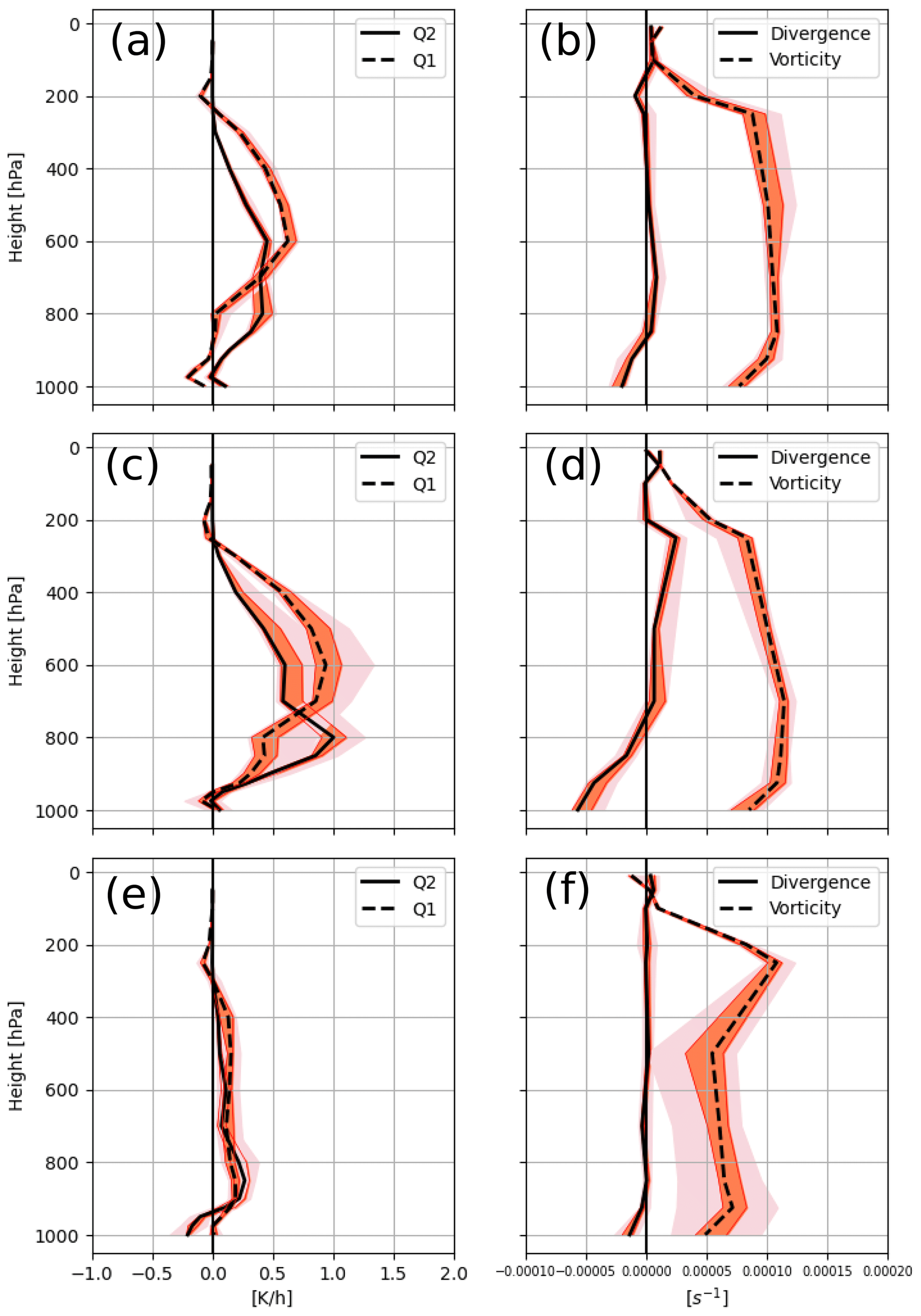
Figure 10 Same as Fig. 8 but for Trixie. Panels (a) and (b) are from 27 October at 12:00 UTC. Panels (c) and (d) are from 28 October at 00:00 UTC. Panels (e) and (f) are from 30 October at 12:00 UTC. These profiles belong to the simulation starting on 27 October. The colour shading is the same as in Fig. 4.

In the case of Trixie, even if the PV anomaly is well reproduced by the SPP-Conv ensemble, compared with the analysis value, the convective heating, reported in Fig. 7f, is not aligned with the PV streamer. This happens in the time step where the cyclone is intensifying before dying out in the ensemble simulations (between 28 and 29 October). When looking at the vertical profiles in Fig. 10a and b, 1 d prior to 28 October, little warming (low values of Q1 and Q2 in the mid-troposphere) and low convergence in the lower troposphere can be noticed, as well as lower values compared with the other two cyclones, nonetheless signalling a brief intensification phase for the cyclones. Indeed, when comparing these results with the minimum core pressure reported in Fig. 4, one can say that Trixie's initial state is well captured by the ensemble starting on 27 October leading to the first cyclone intensification of 28 October. However, if looking at the ensemble mean of the other starting dates, in particular 25 October, the PV streamer and the surface vortex are even more misaligned. Indeed, with the forecast starting date closer to the event, the alignment between the convective heating and the PV streamer is better reproduced (see Fig. S6), which also leads to a better reproduction of the cyclone intensity.

Furthermore, while for Ianos and Zorbas the presence of the cutoff low is well simulated by the ensemble experiments compared with the analysis low (Figs. S3 and S4), this is not the case for Trixie. In the ensemble simulations of Trixie, the cutoff low disappears after 29 October. (Figure S5 shows the different reproduction of the presence of the cutoff low and how it changes with different starting dates.) Its position and intensity had an influence on the track and intensity of Trixie, in accordance with what was suggested in the literature (Pytharoulis et al., 2000). Indeed, in the analysis, two distinct lows are formed separately (Fig. S3) and the first low to form is the one responsible for the Trixie surface vortex, by bringing instability from the upper troposphere to the lower troposphere. In the ensembles, this separation is not well captured. The formation of the second cutoff low prevails and the first one is weakened (Fig. S4), influencing the development of Trixie after its formation, as will be discussed in the following section.

5.2 Cyclone intensification

As underlined in the literature the factor that contributes to the development and intensification to reach a tropical-like state for Mediterranean cyclones is the pairing of the upper-level instability with the lower-level one (Flaounas et al., 2022). More specifically, Carrió et al. (2017) highlight the importance of the upper-level dynamics in intensifying the surface vortex and supporting the tropical transition of the cyclone. This is shown in Fig. 11, which represents the potential vorticity field and the meridional and zonal winds in a cross section of latitude and pressure, at different stages for each medicane for the operational analysis. There, in Fig. 11 a, d, and g, the PV field is shown for the 24 h before the cyclone became tropical-like and it is shown that there is an anomaly of the potential vorticity in the lower troposphere, around 800 hPa, which is a signal for the formation of a surface vortex for all the cyclones accompanied by a production of PV by diabatic processes. In Flaounas et al. (2022), it is summarized that the processes that can underlie the lower-level PV maxima can be the surface fluxes and the release of latent heat due to the organization of strong convective activity. In the upper troposphere, a PV anomaly develops and penetrates from the stratosphere. This happens around the position of the cyclone. After 12 h (Fig. 11b, e, and h) the two PV anomalies, the upper and the lower, start to align. The same mechanism has been recognized in the literature by Cioni et al. (2018) and Miglietta et al. (2017). Finally, the tropical phase is reached when a cyclonic wind circulation completely surrounds the PV anomaly (Fig. 11c, f and i), the so-called PV tower. This is the case for all three cyclones. However, for Zorbas and Trixie deep, convective activity is higher during the intensification phase of the cyclone and then decreases as the maximum intensity is reached, as also recognized by Dafis et al. (2020). This can be seen in the cross sections reported in Fig. 11 where the lower-level PV anomaly is larger in the earlier stages before maximum intensity in Zorbas and Trixie (Fig. 11e and h) compared with Ianos (Fig. 11b). It should be noted that the generation of the diabatic PV anomaly in the lower and middle troposphere is relevant. In fact, as also shown in the previous section, the alignment of the convective heating (taken at 500 hPa in Fig. 7d, e, and f) and the PV anomaly is necessary for the intensification of the cyclones.

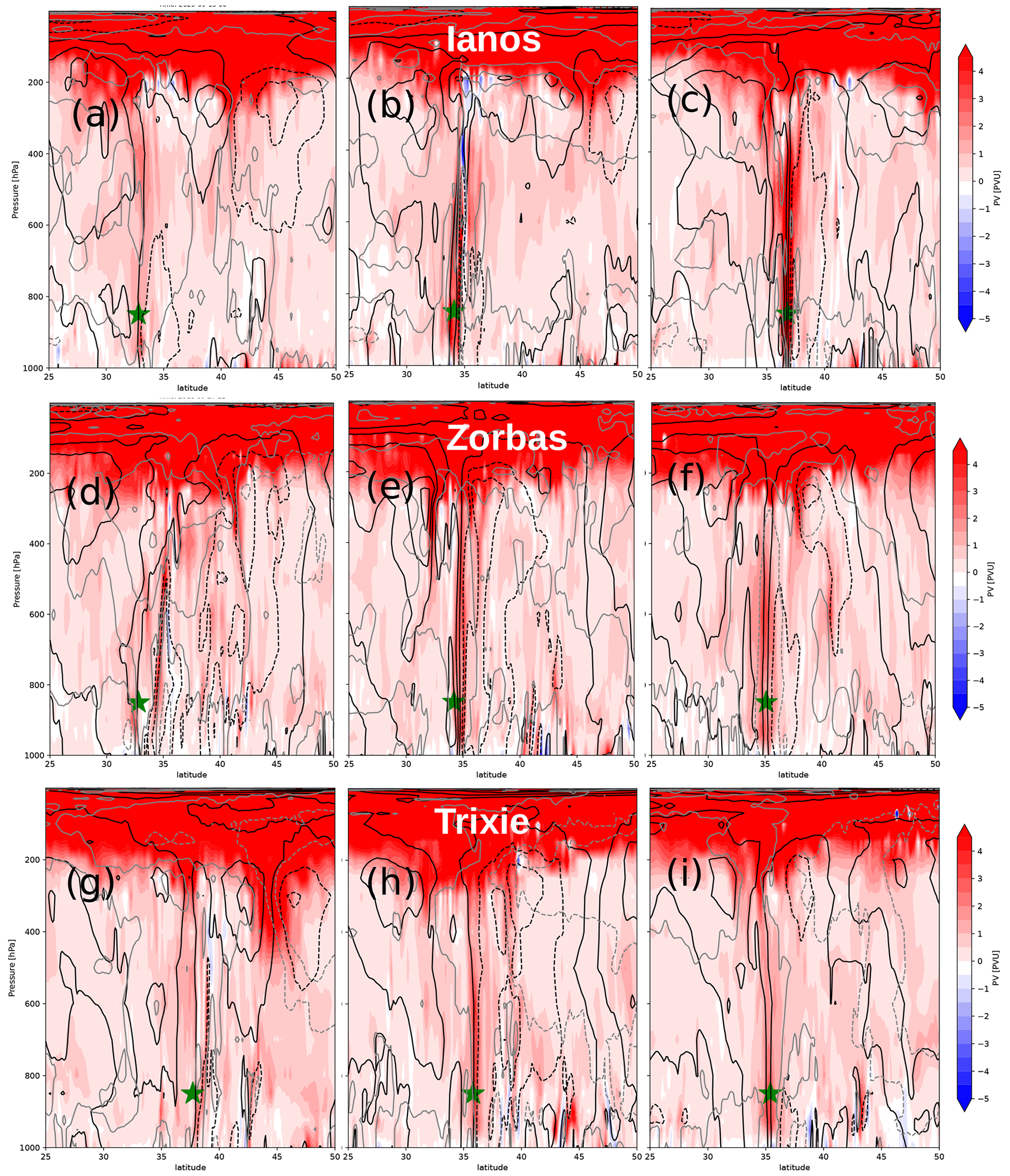
Figure 11 Cross section of the operational analysis potential vorticity field at latitudes from 25 to 50^∘ and pressure. The green star represents the cyclone position. The shaded contours, from blue (negative values) to red (positive values), represent PV. The black lines represent the zonal wind, while the grey lines represent the meridional wind. For Ianos the cross sections shown are for 16 September at 00:00 UTC, 16 September at 12:00 UTC, and 17 September at 00:00 UTC in (a)–(c) respectively. For Zorbas the cross sections belong to 27 September at 12:00 UTC, 28 September at 00:00 UTC, and 28 September at 12:00 UTC in (d)–(f) respectively. For Trixie the cross sections belong to 29 October at 00:00 UTC, 29 October at 12:00 UTC, and 30 October at 00:00 UTC in (g)–(i) respectively.

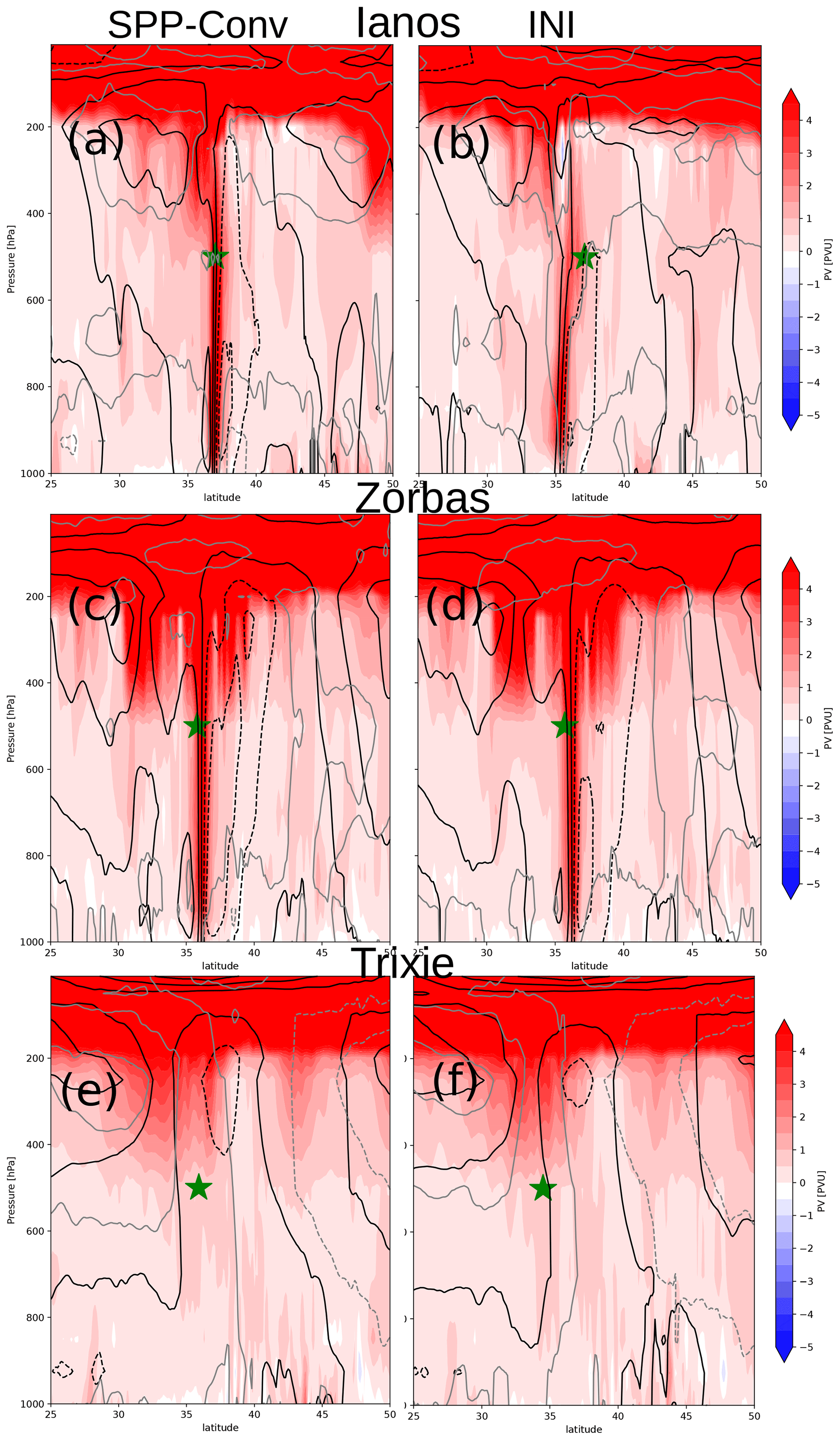
Figure 12 Potential vorticity field cross section in latitude from 25^∘ to 50^∘ and pressure taken in the longitude of the central minimum pressure of the cyclones (green star) as represented by the SPP-Conv and the INI ensemble means in the first and second column respectively. The shaded contours, from blue (negative values) to red (positive values), represent PV. The black lines represent the zonal wind, while the grey lines represent the meridional wind. For Ianos the cross sections shown regard 17 September at 00:00 UTC in (a) and (b). For Zorbas the cross sections belong to 28 September at 12:00 UTC in (c) and (d). For Trixie the cross sections are from 30 October at 00:00 UTC in (e) and (f) respectively.

For Ianos, the tropical-like phase on 17 September is reproduced, with the INI experiment showing a slightly weaker PV than the SPP-Conv ensemble mean (for the simulation starting on 16 September shown in Fig. 12a and b). The tropical-like phase is accompanied by strong divergence above 400 hPa and convergence below 800 hPa (Fig. 8b and d), and by an increase in diabatic heating (Q2 profile) due to condensation. Vorticity increases in the middle and upper troposphere on 17 September (Fig. 8d) compared with the 12 h before. The warm core is sustained for another day and the cyclone begins to dissipate around 19 September. By 20 September (Fig. 8e and f) the cyclone is dying out, with almost no divergence and no convective heating. Comparing Figs. 8c, 9c, and 10c it can be said that the spread is smaller for Ianos, which means less uncertainty about the nature of the medicane compared with Trixie and Zorbas. Moreover, in the case of Ianos, these results compare well with the precipitation field shown in Fig. 5, which is the best simulated among the three medicanes, at least regarding the simulations starting on 17 September. In addition, as mentioned in the analysis of the Hart parameters for Ianos, the presence of a deep warm core is well simulated with decreasing spread and error with starting dates closer to the event (Fig. 6a to d), correlating with the better reproduction of the PV-tower generation. The comparison between the SPP-Conv and the INI ensemble shows that the former experiment produced a slightly more intense cyclone than the analysis and the latter experiment, probably due to the effects of the convective parameterization perturbation.

For Zorbas, on 28 September, the PV values in the two ensemble experiments were higher than the analysis, signalling a slightly more symmetric and intense cyclone (Fig. 12c and d), also in agreement with the results for the Hart parameters shown in Fig. 6e–h. However, the two experiment ensemble means (INI and SPP) are very similar and they both represent the actual presence of a PV tower. Looking at Zorbas' vertical profiles in Fig. 9, it can be seen that the divergence increases above 400 hPa in the tropical phase, around 28 September (Fig. 9d at 12:00 UTC), compared with the previous day (Fig. 9a and b on 27 September at 12:00 UTC). The same is true for the vorticity in the upper and middle troposphere. The warming intensifies and moves into the upper troposphere (Q1 and Q2 profiles in Fig. 9a and c). After 2 d of “tropicalization” the cyclones begin to weaken and by 1 October (Fig. 9e and f) the divergence is almost null and the warming decreases. These results obtained for Ianos and Zorbas are similar to those obtained for tropical cyclones (Geetha and Balachandran, 2016; Lin and Qian, 2019) where intensification occurs. Therefore, it can be said that Ianos and Zorbas go through a tropical phase in the ensemble experiments. There, the heating observed in the simulation is caused by the release of latent heat in the condensation process inside the clouds, as also confirmed by observations for Ianos (Zimbo et al., 2022; Lagouvardos et al., 2022). Indeed, heat fluxes from the sea surface often trigger convection and support intense and persistent diabatic warming through latent heat release from condensation (Carrió et al., 2017). As shown below, the surface fluxes played a role in the intense phase of both Zorbas and Ianos. The spread in Zorbas is reduced by the forecast start date closer to the event (not shown) in favour of the higher values for Q1 and Q2 (shown in Fig. 9c which represents the profiles of the latest start date) which justifies the results for the Hart parameters in Fig. 6e–h. Here, the spread of the upper-level thermal wind is reduced and the error decreases.

Trixie, on the other hand, does not present enough strong surface vortex to match the PV anomaly in the upper level for both experiments (Fig. 12e and f) starting on 25 October. Looking at the other starting date simulations, there appears to be a stronger lower-level instability (not shown). However, this cannot be sustained by the simulation. For Trixie, indeed, the deep warm core state is never reached. As said before, this cyclone is the weakest and it can intensify only on 28 October in the ensemble simulations (Fig. 10c and d at 00:00 UTC). The convective heating represented by a positive Q1 and Q2 is weaker compared with the other cyclones (Figs. 8 and 9) and the maximum is located in the mid-troposphere, signalling a shallow warm core. The divergence, which is increasing compared with the previous 12 h (Fig. 10b and d), is not accompanied by an increase in vorticity and it starts at mid-troposphere. The warming is weak and there is no divergence (Fig. 10e and f). Trixie presents the highest spread regarding the warming, also mirroring the results from the Hart parameters reported in Fig. 6i to l. The warming, which does not correspond to a shallow warm core, is reached only on 28 October but is absent on 30 October, when Trixie is supposed to become a tropical-like cyclone (Dafis et al., 2020). Thus, the Hart parameter values are justified by the absence of upper-level warming for Trixie. This is also correlated with the minimum core pressure development presented in Fig. 4 and for the accumulated precipitation in Fig. 5, where every ensemble experiment diverges from the analysis and observations after 29 October. These results indicate that Ianos and Zorbas are simulated mostly with the right tropical-like phase, with almost the right timing (12–24 h of delay as mentioned above), while the ensemble simulation for Trixie fails to reproduce the right intensification of the cyclone, simulating a shallow warm core on 28 October and missing the deepening on 30 October.

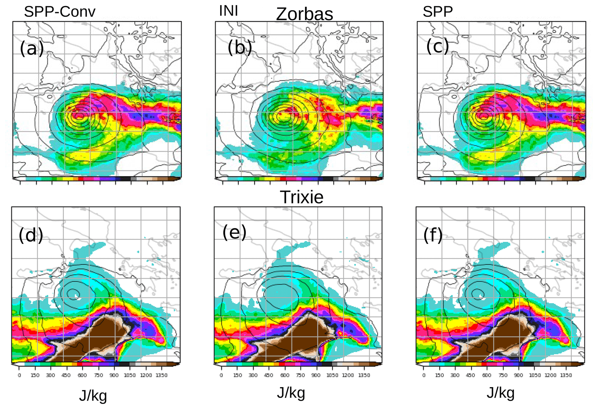
Figure 13 Convective available potential energy (J kg⁻¹) (in colours) and mean sea level pressure (in lines) for the three ensemble experiments' ensemble means. For Zorbas 28 September at 12:00 UTC is shown in (a)–(c) for the simulation starting on 27 September. For Trixie 28 October at 12:00 UTC is shown in (d)–(f) for the simulation starting on 27 October.

It seems that the ensembles have presented issues for Trixie in reproducing the presence or absence of PV anomalies generated by diabatic processes and the latter interaction with the upper-level one. In order to understand this latter aspect, the convective activity in the three medicanes has first been analysed by means of the convective available potential energy (CAPE). The main result is weaker convection indicated by a weaker CAPE in Trixie. Indeed, in Fig. 13 there is a comparison between CAPE around the cyclone centre for Zorbas and Trixie at the intensification tropical-like state. In the ensembles, the reduced convective activity near the centre reported in Fig. 13 for Trixie underlines the lower energy conversion from diabatic heating. Such a situation can be ineffective in driving the cyclone to a state in which it is able to self-sustain by the wind-induced surface fluxes (Emanuel, 1986) and the transition to the tropical-like cyclone being degraded as already found in Koseki et al. (2021).

This is correlated with the effect of the surface fluxes, which are much higher in the case of Zorbas and Ianos compared with Trixie (Fig. S7). Indeed, also the total heat flux at the surface (the sum of the sensible and latent heat flux) has been inspected. In Fig. S7 it is made clear that in the ensembles for Ianos and Zorbas the surface fluxes amount to around 500 W m⁻² and are concentrated for Ianos around the centre and for Zorbas are much more spread out. For Trixie, instead, the values are much lower and not at all comparable with the other cyclones. In general, by 29 October, in the Trixie simulation, the convection is weakening and by 30 October is absent in the ensemble experiments compared with the situation in the analysis. Thus, this reduced CAPE in the ensemble simulations is signalling a simulated weaker low-level vortex and a lower PV anomaly.

The surface level production of PV in Trixie is not enough to match with the upper tropospheric high PV field as reported in Fig. 12e and f, or they are not in phase. In the ensemble simulations starting on 27 October, the amount of diabatically generated PV comparable to that in the analysis is not able to align with the upper-level one, even though the alignment is better captured with starting dates closer to occurrence (Fig. S6). This pertains to both the INI and SPP experiments, as mentioned before, meaning that the production of the right diabatic processes is equally sensitive to initial conditions and to physical and, more specifically, convective processes. The analysis points out that the cyclone dies before 30 October due to the low-level vortex being too weak and not able to interact properly with the upper-level disturbances. Actually, the surface vortex disappears with the weakening of the upper-level cutoff low, and due to the absence of a reinforcement of the lower-level PV production by the upper-level one, meaning erosion of PV by the presence of intense diabatic processes, as is happening, for instance, in Zorbas (Portmann et al., 2020). First, as mentioned in the previous section, in the ensemble simulations of Trixie (both INI and SPP), the cutoff low that was crucial for the formation of the surface cyclone disappears after 29 October and the formation of the second cutoff low weakens the first. With the weakening of the cutoff low, Trixie starts lowering its intensity. Only a few members can follow the weak cutoff low (Fig. S3). This has had an impact on the simulation of the already weak cyclone, Trixie. Indeed, it is hypothesized that Trixie is formed as a lower-level vortex mainly due to the thermodynamic disequilibrium generated by the upper-level cutoff low. If the latter is not well simulated, being weaker, it is not able to sustain the surface vortex. Second, when the surface level vortex is better reproduced, the misalignment with the upper-level PV anomaly does not permit reinforcement of the convection. Homar et al. (2003) and Cioni et al. (2018) showed that the upper-level PV structure indirectly acts on the cyclone deepening through a modification of the surface circulation.

As mentioned above, the simulation of strong convective activity seems to be important in all three cyclones, which is associated with latent heat release, developing in the central region of the cyclones (Figs. 8, 9, and 10). As recognized in the literature, either the surface fluxes or convective activity can predominate in the intensification of the surface level vortex, as identified for different medicanes (Davolio et al., 2009; Miglietta et al., 2017; Chaboureau et al., 2012; Fita and Flaounas, 2018). While surface fluxes seem to have also played a role in the intensification of both Ianos and Zorbas (Fig. S7), in the case of Trixie specifically deep moist convection seems to be the main mechanism leading to the maintenance and deepening of the system, due to the interaction of convection with the upward forcing induced by the PV streamer (Chaboureau et al., 2012). Indeed, for Trixie it is the long-lasting deep convective activity that may have played an important role in their intensification later than their genesis time, as also recognized by Dafis et al. (2020), and its weakening or even absence compromises the forecast, as happens in the presented ensemble experiments. While the tracking is mainly influenced by the position of the cutoff low and the PV streamer position, the simulation intensification phase and timing are dependent on how the convection is reproduced and interacts with the upper-level PV structure.

5.3 The role of the sea surface temperature

By looking at the sea surface temperature (SST) anomaly, it is found that it is higher for Zorbas (Ianos is once again affected by the SST anomaly similarly to Zorbas) upon formation compared with Trixie, as reported in Fig. 14 which represents the ensemble mean anomaly of the SPP-Conv and INI experiments for Zorbas and Trixie for comparison. On one hand, for Zorbas (Fig. 14a, b, and c) the SST is anomalously high compared with the climatological SST of September (obtained by using the ERA5 reanalysis SSTs over the Mediterranean basin from 1991 to 2020), of on average 2 ^∘C. On the other hand, for Trixie the anomaly (with respect to the climatological SST of October) decreases, and in the area of cyclone formation it is very weak compared with Zorbas (Fig. 14d, e, and f). This means that the air–sea temperature contrast did not play as crucial a role in Trixie generation and maintenance as it did for Ianos and Zorbas, probably resulting in weaker low-level vortex altogether (mirroring what is shown in Fig. S7 for the surface fluxes).

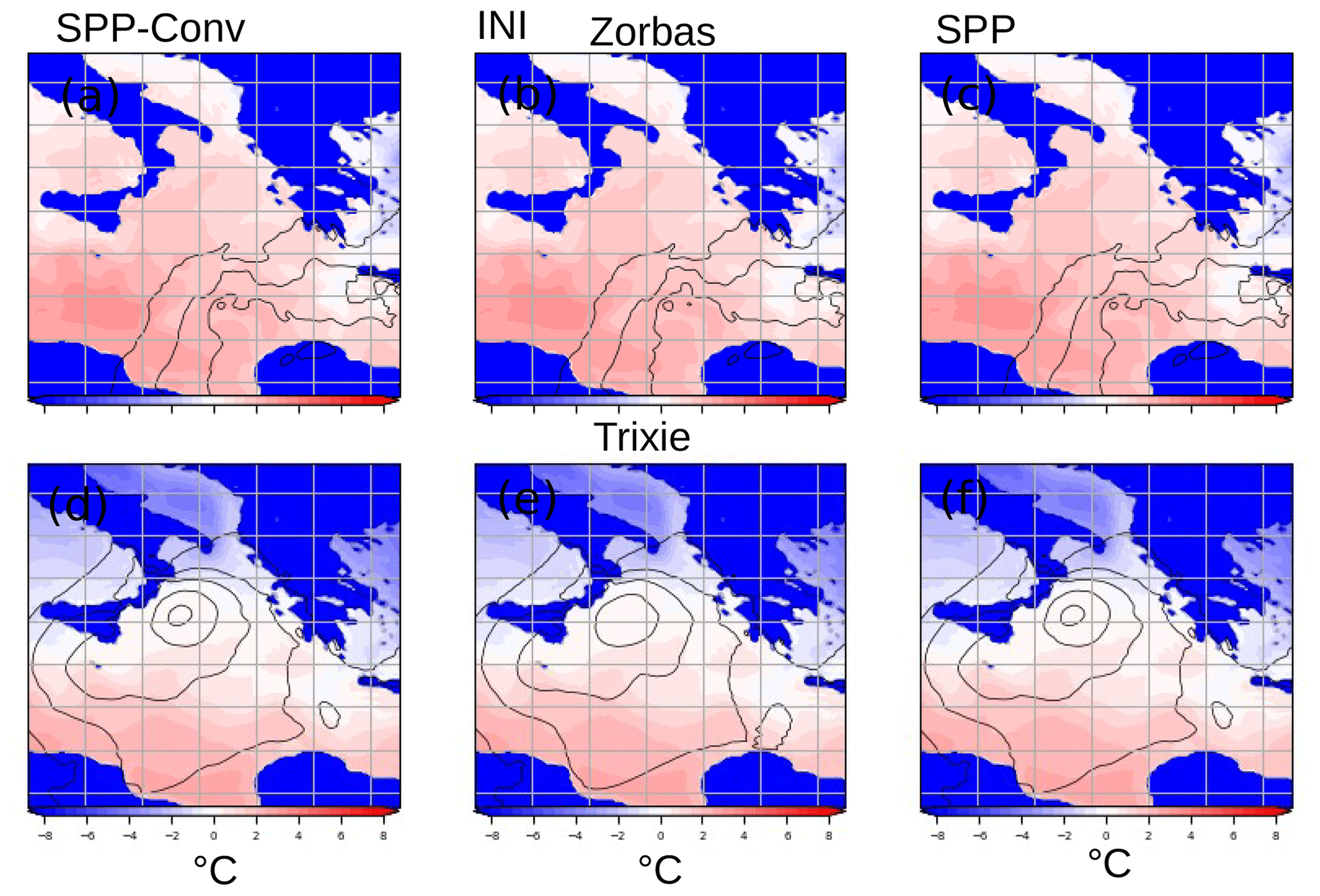
Figure 14 Sea surface temperature anomaly (^∘C) (in colours) and mean sea level pressure (in lines) for the three ensemble experiments' ensemble means. For Zorbas 27 September at 00:00 UTC is shown in (a)–(c) for the simulation starting on 27 September. For Trixie 28 October at 00:00 UTC is shown in (d)–(f) for the simulation starting on 27 October.

Indeed, the ensemble experiments' results compare fairly well to the operational analysis for the SST anomaly for the three medicanes (not shown), underlining the relative importance of the air–sea interaction in the tropicalization of certain Mediterranean cyclones. Noyelle et al. (2019) found that the SST state has a strong influence on the medicanes' intensities and that increased SSTs lead to greater probabilities of tropical transitions, stronger upper-level warm cores, and lower minimum pressure, by influencing the intensity of fluxes from the sea, which leads to greater convective activity before the storms reach their maturity. The higher surface temperatures in Ianos and Zorbas help feed the medicane the moisture, through surface fluxes (Pytharoulis, 2018), allowing the convection to develop more effectively (Koseki et al., 2021; Cioni et al., 2018).

6 Discussion and conclusion

Predicting and simulating medicanes is a difficult task due to them being extreme events found near the tail of the forecast distribution (Majumdar and Torn, 2014) and due to the complexity of the processes involved. The specific barriers to predictability and the atmospheric conditions that lead to the formation and evolution of medicanes are not fully understood. Research using multi-physics approaches has found that the track, intensity, and duration of medicanes are heavily sensitive to factors such as convection, microphysics, and boundary-layer parameterizations (Ragone et al., 2018; Miglietta et al., 2015). Indeed, this study is one of the first steps towards understanding this sensitivity by using ensemble forecast simulation.

The analysis was focused on three medicanes using the ECMWF model IFS ensemble forecast system. In addition to the operational ensemble forecast, the TOT ensemble, some other experiments have been carried out: the initial-condition perturbation ensemble, INI; and two ensembles with SPP, in one case perturbing only the parameters of the convection parameterization, SPP-Conv, and in the other perturbing the parameters of all relevant physical parameterizations, SPP. The approach used was aimed at analysing the tracks and intensity, i.e. central pressure, precipitation, and parameters characterizing the thermal structure of the cyclones. Second, the processes behind the generation and development of the cyclones have been analysed in conjunction with the previous analysis.

The result of this study, compared with previous ones (Di Muzio et al., 2019; Chaboureau et al., 2012; Pantillon et al., 2013) which used only the operation ensemble forecast of ECMWF, points out the benefit of using the SPP ensemble forecast compared with just perturbing the initial conditions. The use of SPP, and in particular the perturbation of convective parameters (SPP-Conv), was found to compare well with the INI and TOT experiments in terms of tracking, cyclone intensity, and precipitation. Similar results have been reported in Ollinaho et al. (2017), especially regarding precipitation. The experiments are usually underdispersive in terms of tracking position, although the TOT experiment gives better results. Indeed, the ensemble forecast TOT has proven to be the best in terms of spread and error compared with the tracking, intensity, and precipitation of cyclones. This is due to the inclusion of the model's physics perturbation, in line with what was found in Lang et al. (2021). The ensemble spread and mean are generally lower in the SPP experiments. For instance, the analysis of the thermal structure and symmetry shows that for the upper-level thermal wind, the smaller spread is obtained in most cases in the SPP-Conv experiment (in particular at later forecasts). Nonetheless, the two SPP ensembles are able to produce the same spread as the initial-condition perturbation experiment at later time steps, highlighting the benefit of introducing physical parameter perturbations, especially with respect to convection, compared with using only perturbations of the initial conditions (Lang et al., 2012; Ollinaho et al., 2017). Moreover, the similarity of the SPP and the SPP-Conv results, especially for the thermal structure and thermal asymmetry, highlights that the uncertainties linked to the convection parameterization are predominant in the simulation of these types of phenomena, confirming previous results (Pytharoulis, 2018; Fink et al., 2012; Wimmer et al., 2022). Finally, with respect to the above-mentioned cyclone characteristics, it is found that there is a common gradual decrease in the error with the forecast starting date closer to the occurrence. This is consistent for all three ensemble experiments and it is specific for Ianos and Zorbas. For Trixie this decrease in the error is weaker and, in some cases, non-existent. Indeed, as pointed out in the results, the simulation of this particular cyclone can be considered as a missed forecast (as shown by the track in Fig. 1 and the intensity in Fig. 4).

Specifically, regarding the reproduction of the minimum central pressure by the ensemble forecasts (Fig. 4), there is generally a time shift in the reproduction of the minimum intensity, where both the Ianos and Zorbas ensemble means reach the maximum intensity with a delay. Since the delay decreases as the forecast starting date gets closer to the event, this is due to the improved initial conditions. Indeed, it is found that the maximum intensity is reached when the upper-level PV streamer and the surface-level vortex are aligned, and the latter is better captured by starting the simulation closer to the cyclone's onset. This is consistent with what was found by Flaounas et al. (2015) where they underlined that the intensity of the surface cyclone increases while the streamer is on the western side of the cyclone and begins to decrease as the streamer is wrapping over its centre. It is noteworthy that for Zorbas the intense phase (i.e. low values of minimum core pressure) is maintained for a longer period, compared with the operational analysis, as underlined by the minimum core pressure trend in Fig. 4 and by the PV tower reported in Fig. 12. This is probably due to the fact that most members (especially regarding the SPP ensembles) spend most of their lives at sea and do not cross land over Greece, thus managing to sustain themselves for a longer period through condensational heating and air–sea interaction.

Furthermore, by looking at the simulated precipitation distribution compared with the GPM-IMERG satellite observations, it is shown that only for Ianos is the precipitation field well reproduced by the ensembles, with the SPP experiment being slightly more intense than the others. Even if the GPM-IMERG dataset tends to overestimate the precipitation over the Mediterranean (Peinó et al., 2022; Caracciolo et al., 2018), the simulated precipitation for Zorbas and Trixie is too weak. However, it is discussed that in general, the precipitation maximum compares better with the forecasts' starting date closer to the occurrence; thus, for Zorbas, starting the ensemble forecasts on 28 September would have shown better-simulated precipitation. It could be argued that a finer resolution than a 9 km resolution would improve the reproduction of the intensity and track of the tropical-like Mediterranean cyclones. A recent single forecast experimental tropical cyclone with simulations at 4 km resolution by Majumdar et al. (2023) revealed that the 4 km simulations produce deeper and more realistic tropical cyclones in terms of radial wind structure, compared with the observations, than the 9 km forecasts. However, in the aforementioned work done within the DestinE project (Gascón et al., 2023), preliminary simulations carried out with IFS at 4 km resolution did not show any significant changes in the simulated tracks and intensity of Medicanes, except for slightly more intense winds. This applies to both Trixie (https://confluence.ecmwf.int/x/soQvEQ, last access: 26 October 2023) and Ianos (https://confluence.ecmwf.int/x/soQvEQ, last access: 26 October 2023) where the 9 and 4 km resolution simulations are roughly equivalent.

It is shown that for Ianos and Zorbas the forecasts are accurate at reproducing both the thermal structure and symmetry of the cyclones compared with the analysis value. The only exception to the reasonable reproduction of the storm thermal structure is the upper-level thermal wind in Trixie (Fig. 6a, c, and e). This means that for Trixie, where the analysis value reported the presence of a warm core ($-V_{\mathrm{T}}^{\mathrm{U}}=\mathrm{25}$ in Table 2), the three ensemble forecast presents a cold core cyclone (negative $-V_{\mathrm{T}}^{\mathrm{U}}$ values). This, together with the underestimation of the deepening of the cyclone, can explain the simulated precipitation being weaker than the observations since the simulated cyclone is not able to reach the warm core; thus, the convective heating is lower, affecting the simulation of the precipitation. From the Q1 and Q2 profiles, it is evinced that the cyclone seems to intensify around 28 October and to die out by 30 September, when it should have entered the tropical phase, as mentioned in Dafis et al. (2020).

Indeed, through tracking, it was verified that with regard to the Trixie simulation, there is a southeastward shift of the trajectory with respect to the analysis (Fig. 1). A lower spread in the tracked position was found for Zorbas and Ianos compared with Trixie, but the error of Trixie exceeds 800 km. This is attributable to the fact that the ensemble forecast starts too early with respect to the cyclone intensification phase for Trixie. This result, in particular, aligns with previous studies that had pointed to Trixie's low occurrence probability up to 2 d earlier (Di Muzio et al., 2019). Indeed, There is an inherently low probability of medicane occurrence (as seen in Di Muzio et al., 2019) and the development of a warm core cyclone depends on many factors, large-scale factors and surface fluxes, that can be improved by the initial conditions of a preexisting cyclone.

In order to evaluate the obtained results, an investigation of the development processes and their simulation were linked to the forecasts' track position and intensification of each cyclone. First, it has been pointed out that Ianos, Zorbas, and Trixie all require the presence of a PV streamer together with a deep cutoff low in order to form. This underlines the nature of these cyclones as being born in a baroclinically unstable environment. This is initially reproduced reasonably well, although specifically in the case of Trixie, the ensembles may have started too early to capture the interaction between the two, making Trixie a weaker cyclone and ultimately leading to its ending. As pointed out in the previous section, the cutoff low which contributes to the development of Trixie quickly weakens in the ensemble simulations after 29 October and is then shut down in favour of another one that crossed the Ionian Sea (Figs. S4 and S5).

Furthermore, it has been shown that after the formation of the three cyclones, the operational analysis represents a clear interaction between the surface level vortex and the PV anomaly in the upper troposphere in all three cases, the PV tower, in order for them to intensify and eventually reach “tropical-like” features (Carrió et al., 2017; Cioni et al., 2018; Flaounas et al., 2022). This is present in the ensembles (both for SPP and INI) in the case of Ianos and Zorbas, where the upper-level PV anomaly brought by the PV streamer is able to match with the lower-level PV production by diabatic processes. As also pointed out, this surface cyclone is sustained by convective heating release by condensation, with surface fluxes supporting the cyclone in the most intense phase along with convective activity (Fig. S7). In the case of Ianos, the convective activity peaks during the most intense phase, as underlined by the PV anomaly in the PV cross section in Fig. 11, while in the case of Zorbas, convective activity is present also before the cyclone tropical-like phase (as also underlined by the PV anomaly in Fig. 11). The ensemble simulated cyclones are sensitive to the positioning of the PV streamer, which, as observed in the literature, has a clear impact on the simulation of the medicane. In the case of Zorbas, as noted in Portmann et al. (2020), a westward shift of the PV streamer leads on average to weaker cyclones, which can be observed in the ensemble mean of Zorbas in Fig. 4. The displacement of the PV streamer is linked to the alignment with the surface level and the consequent creation of a PV tower. Furthermore, the intensity of the PV anomalies, as well as the height reached by the 2 PVU isosurface, may have played a role in the cyclone's greater or lesser intensity. In fact, in the case of Ianos, it can be argued that the cyclone is more intense in the ensembles compared with the analysis observations due to the higher simulated PV anomaly and deeper PV streamer. In other studies, also using the ECMWF ensemble forecasting system (Chaboureau et al., 2012), it was found that later forecasts are able to capture better the thermal structure of the medicanes, due to the lower uncertainty of the positioning of the PV streamer connected to the generation of the medicane. In general, in our study it is assessed that the earlier the starting date, the greater the misalignment (or the worse the positioning of the upper-level disturbance) between the lower and the upper PV production. This is true, particularly in the case of Trixie, where on the simulation starting too early, on 25 October, the lower-level PV production is absent, and for the simulations starting on 26 and 27 October it is very weak and not able to be reinforced by the upper-level one.

Trixie is also a weaker medicane compared with Ianos and Zorbas (the central minimum pressure of Trixie is lower than that of the other two cyclones, as reported in Table 2), influencing the simulations. In a recent study by Panegrossi et al. (2023), while Ianos and Zorbas have been recognized as two of the most intense medicanes, Trixie has been characterized as one of the weakest, not even reaching the status of deep warm core, as established by looking at passive microwave measurements and products. Here, it has been shown that (a) the surface fluxes in the phase of tropicalization and intensification are lower than the other medicanes; (b) the SST anomaly in the case of Trixie was low both in the analysis and in the ensembles, yielding to a weaker cyclone; and (c) Trixie tends to shut off when the cutoff low vanishes in the simulations and generally tends to follow the PV streamer position. This makes it subject to being more dependent on the simulation of large-scale processes. More specifically, the lower-level PV production present in the analysis in Fig. 11 is absent in the simulations in Fig. 12. Since the surface fluxes and the anomaly of SST do not play a role, this makes the convective instability brought by the cutoff low necessary to sustain the cyclone convection. The deep cutoff low absence in the simulations can be linked to the medicane missing development in the case of Trixie. This is supported by the findings of Fischer et al. (2017), who hypothesized that tropical cyclone intensification rate after tropical cyclogenesis, in environments of upper tropospheric troughs, is closely linked to the structure and temporal evolution of the upper-level trough.

Going back to the medicane classification, the three medicanes seem to belong to different medicane categories. Ianos and Zorbas seem to belong to the one in which baroclinicity is important only in the initial stage and positive feedback between the latent heat release and the air–sea interactions is behind their intensification through Flaounas et al. (2022). Trixie seems to belong to the one in which baroclinic instability plays an important role throughout the cyclone's lifetime and most of the intensification is due to convection (Fita and Flaounas, 2018). Thus, one of the outcomes of this study is that the ensemble forecasting of ECMWF is likely able to better capture the tropical-like features of the first category of medicanes. The investigation of this will be the subject of further study, also considering a greater number of medicanes. This analysis also underlines the different sensitivity of the diabatic processes in the simulation of these medicanes, because it makes it clear that convective heating has played a major role in the intensification of the cyclones and, when absent, is linked to the disappearance of the cyclone itself, as in the case of Trixie.

In conclusion, this study confirms that similar processes are at play in the development of Mediterranean tropical-like cyclones and the predictability of these cyclones is linked to not only the reproduction of the precursor events (namely the deep cutoff low) but also to the interaction of the upper-level dynamics with the lower-level ones (namely the PV streamer and the lower-level PV production), in a similar way. This work, as urged in the literature (Dafis et al., 2020; Pytharoulis, 2018), underlines the relative importance of the upper tropospheric troughs and PV streamer interactions with the troposphere for medicanes not only in one specific case, as often done in the literature (Portmann et al., 2020; Chaboureau et al., 2012; Cioni et al., 2018), but extending the analysis at least to a few different cases.

Finally, as discussed in Flaounas et al. (2022), the representation of cloud adiabatic processes is often believed to be a source of forecast uncertainty but dominated by the one created by initial conditions. This study, by comparing ensemble forecasts with the account of initial-condition perturbation only and of physical parameterization only, underlines that the uncertainty produced by both ensembles is actually similar.