Spatiotemporal modeling of air pollutant concentrations in Germany using machine learning

Machine learning (ML) models are becoming a meaningful tool for modeling air pollutant concentrations. ML models are capable of learning and modeling complex nonlinear interactions between variables, and they require less computational effort than chemical transport models (CTMs). In this study, we used gradient-boosted tree (GBT) and multi-layer perceptron (MLP; neural network) algorithms to model near-surface nitrogen dioxide (NO₂) and ozone (O₃) concentrations over Germany at 0.1^∘ spatial resolution and daily intervals.

We trained the ML models using TROPOspheric Monitoring Instrument (TROPOMI) satellite column measurements combined with information on emission sources, air pollutant precursors, and meteorology as feature variables. We found that the trained GBT model for NO₂ and O₃ explained a major portion of the observed concentrations (R²=0.68–0.88 and RMSE=4.77–8.67 µg m⁻³; R²=0.74–0.92 and RMSE=8.53–13.2 µg m⁻³, respectively). The trained MLP model performed worse than the trained GBT model for both NO₂ and O₃ (R²=0.46–0.82 and R²=0.42–0.9, respectively).

Our NO₂ GBT model outperforms the CAMS model, a data-assimilated CTM but slightly underperforms for O₃. However, our NO₂ and O₃ ML models require less computational effort than CTM. Therefore, we can analyze people's exposure to near-surface NO₂ and O₃ with significantly less effort. During the study period (30 April 2018 and 1 July 2021), it was found that around 36 % of people lived in locations where the World Health Organization (WHO) NO₂ limit was exceeded for more than 25 % of the days during the study period, while 90 % of the population resided in areas where the WHO O₃ limit was surpassed for over 25 % of the study days. Although metropolitan areas had high NO₂ concentrations, rural areas, particularly in southern Germany, had high O₃ concentrations.

Furthermore, our ML models can be used to evaluate the effectiveness of mitigation policies. Near-surface NO₂ and O₃ concentration changes during the 2020 COVID-19 lockdown period over Germany were indeed reproduced by the GBT model, with meteorology-normalized near-surface NO₂ having significantly decreased (by 23±5.3 %) and meteorology-normalized near-surface O₃ having slightly increased (by 1±4.6 %) over 10 major German metropolitan areas when compared to 2019. Finally, our O₃ GBT model is highly transferable to neighboring countries and locations where no measurements are available (R²=0.87–0.94), whereas our NO₂ GBT model is moderately transferable (R²=0.32–0.64).

1 Introduction

Air pollution is a major threat to human health and impacts ecosystems (Bell et al., 2011; Lelieveld et al., 2015; Zhang et al., 2019; Xie et al., 2019). Based on the source of the pollution, air pollutants are classified as being primary (directly emitted from anthropogenic or natural sources) or secondary (formed through complex atmospheric chemical reactions). Near-surface nitrogen oxide (${\mathrm{NO}}_x=\mathrm{NO}+{\mathrm{NO}}_{\mathrm{2}}$) is a primary air pollutant emitted largely by fossil-fuel-consuming sectors such as vehicles, industries, and power plants, but there are also natural sources such as lightning, soil emissions, and biomass burning. Near-surface ozone (O₃) is a secondary air pollutant produced solely by the photolysis of NO₂ (nitrogen dioxide) in the presence of sunlight (Crutzen, 1988; Council, 1992).

Tropospheric NO_x and O₃ are chemically strongly coupled via complex atmospheric chemical reactions (Jacob, 1999). The majority of NO_x, from primary sources such as fossil fuel combustion, is emitted in the form of nitric oxide (NO), which rapidly converts to NO₂ by reacting with O₃. In turn, O₃ and NO are generated again by the photolysis of NO₂, thus forming a null cycle. Therefore, the amount of sunlight present and the total concentration of NO_x determine ozone production via this NO_x null cycle. In addition, the oxidation of volatile organic compounds (VOCs) can alter the $\mathrm{NO}/{\mathrm{NO}}_{\mathrm{2}}$ ratio. The presence of the hydroxyl radical (OH) initiates the VOC oxidation process, followed by the formation of hydro- and organic peroxy radicals. These radicals convert NO to NO₂ and form additional O₃, while also converting HO₂ back to OH, thus forming a catalytic cycle known as the HO_x catalytic cycle. However, ozone production is nonlinear in relation to its precursors (NO_x and VOC) due to termination reactions that occur within the catalytic cycle (Lin et al., 1988; Nussbaumer and Cohen, 2020; Pusede and Cohen, 2012; Pusede et al., 2014). To that end, the response of ozone production is categorized into three regimes, namely NO_x-saturated (high NO_x with low VOC); NO_x-limited (low NO_x with high VOC); and transitional (Sillman et al., 1990; Sillman, 1999). In the NO_x-saturated regime (typically urban areas), ozone production is inversely proportional to NO_x concentration, whereas ozone production is directly proportional to VOC concentration. However, in NO_x-limited regimes (typically rural areas), ozone production is directly proportional to NO_x concentration, whereas VOCs have little effect on ozone production. This complex ozone production vs. precursor emission response is also evident in real-time observations, such as urban weekend ozone levels being higher than weekday levels (Sicard et al., 2020) and high-ozone levels during public holidays and national shutdowns (e.g., the COVID-19 lockdown), due to low NO_x emissions (Balamurugan et al., 2021, 2022b).

Chemical transport models (CTMs) are commonly used to study air pollution and its drivers (Hu et al., 2016; Lou et al., 2015), but these models are dependent on emissions as represented in emission inventories (Pisoni et al., 2018). Emission inventories are typically developed using the bottom-up method, based on data such as economic activity, fuel consumption, and traffic density (McDuffie et al., 2020; Osses et al., 2022). However, bottom-up emission inventories can be highly uncertain due to inaccuracies in the data used in the bottom-up method, especially from unaccounted-for sources (Chen et al., 2020; Crippa et al., 2019; Forstmaier et al., 2023; Trombetti et al., 2018). Because of the significant computational effort and storage space requirements, CTMs often perform at a coarse spatial resolution, making it unable to solve fine transport and chemical mechanisms, particularly over complex topography (Singh et al., 2021). Machine learning (ML) models have been shown to be an effective complement to these computationally expensive CTMs (Vlasenko et al., 2021). The performance of machine learning models for modeling air pollutants is promising (Balamurugan et al., 2022a; Cheng et al., 2022; Lee et al., 2020; Li et al., 2023; Liang et al., 2020; Liu et al., 2022; Zaini et al., 2022; Zhao et al., 2023). Meteorological variables such as solar radiation and temperature have been shown to be important parameters in near-surface ozone modeling using machine learning (Diao et al., 2021; Hu et al., 2021). Meteorological conditions influence the concentration of O₃ both directly and indirectly. Solar UV radiation is responsible for the photolysis of O₃ precursors (NO₂ and VOCs). Temperature directly influences the photochemical reaction rate. Furthermore, meteorology influences biogenic and fuel-leak-related VOC emissions (exponentially proportional to temperature), which account for a significant portion of total VOC emissions (Guenther et al., 1993). In addition to meteorology, when the emission source information is included, ML models predict near-surface NO₂ very well (Ghahremanloo et al., 2021; De Hoogh et al., 2019).

In situ air quality measurements are sparse and concentrated primarily in urban areas. Recent advancements in satellite remote sensing allow us to analyze urban and non-urban air quality with adequate spatiotemporal coverage; however, they typically only measure the total or tropospheric column of specific air quality species, making it difficult to interpret people's exposure to the near-surface air pollutant concentration. Therefore, in this study, we trained two ML models for near-surface NO₂ and O₃ concentrations over Germany using available information on proxies for near-surface air pollutants (satellite column measurements) and emission sources, precursors of air pollutants, and meteorology. Many recent studies, similar to ours, have attempted to model near-surface NO₂ and O₃ concentrations at national or regional scales (De Hoogh et al., 2019; Kang et al., 2021; Kim et al., 2021; Li et al., 2020; Zhu et al., 2022); there are, however, very few attempts over Germany. To the best of the authors' knowledge, only one study (Chan et al., 2021) used the TROPOspheric Monitoring Instrument (TROPOMI) satellite NO₂ tropospheric column measurements and other auxiliary information (e.g., meteorology) to model near-surface NO₂ concentrations over Germany using a multi-layer perceptron (MLP) model. Furthermore, previous studies have focused on a single pollutant (e.g., NO₂), whereas in this study, we model and analyze the spatiotemporal variations in both NO₂ and O₃, which are chemically strongly coupled. In terms of anthropogenic emissions, we also evaluate the ML model performance of NO₂ and O₃ during the 2020 COVID-19 lockdown period, which serves as a natural experiment period with significantly lower primary anthropogenic emissions (Gensheimer et al., 2021).

2 Study region, data sets, model, and method

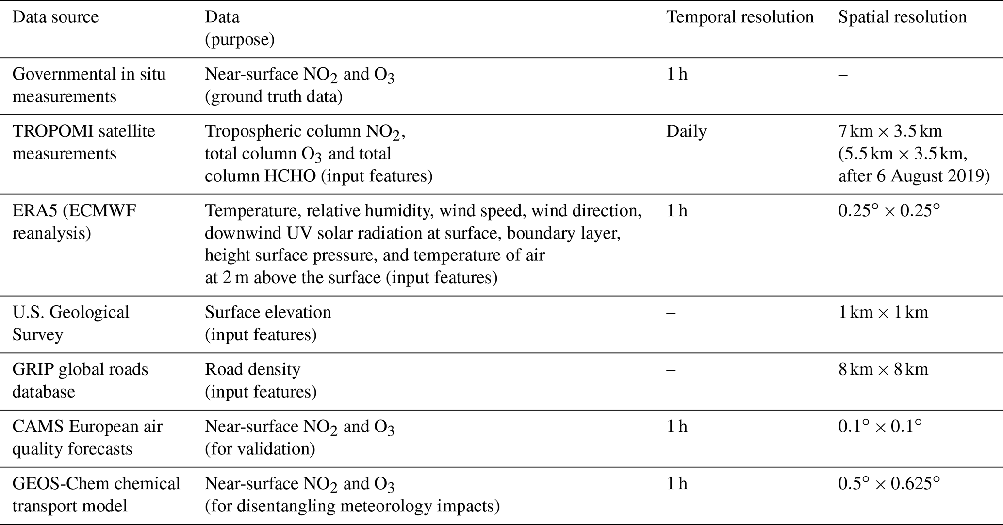
All data sets used in this study, and their spatial and temporal resolutions, are summarized in Table 1.

Table 1 Data sets and related information used in this study.

2.1 Study region and near-surface NO₂ and O₃ measurements

We focused on the spatial domain of 5–15^∘ E and 47–55.5^∘ N, particularly over Germany. Near-surface NO₂ and O₃ data from measurement stations across Germany were used in this study. However, not all measuring stations collect data on both pollutants; there are fewer stations measuring O₃ than those measuring NO₂. There were also temporal gaps in the measurement data. Therefore, we only considered stations that had more than 80 % data coverage during the study period. In the end, we considered 321 stations for modeling NO₂ and 256 stations for modeling O₃. The selected measurement stations are located throughout the entire country and are situated in high-traffic, industrial, and background locations (Fig. 1 and Table A1).

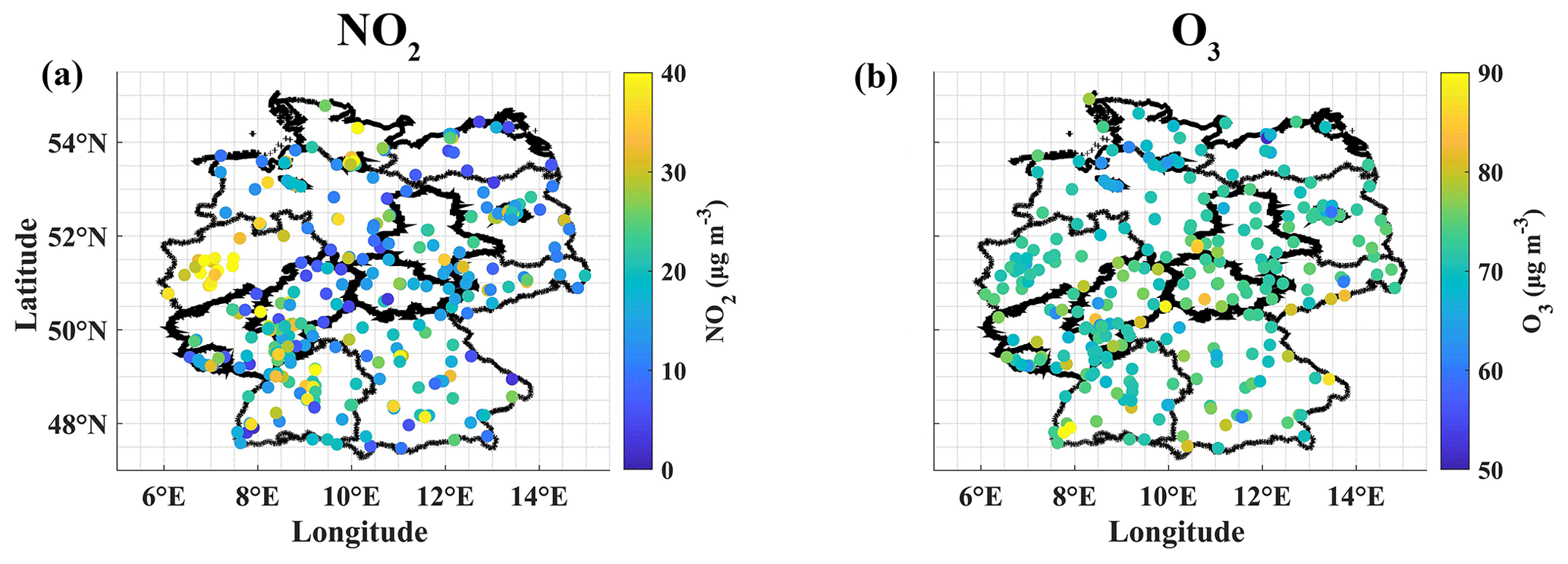
Figure 1 Locations of near-surface NO₂ (a) and O₃ (b) measurement stations considered in this study. The color bar depicts the mean of near-surface NO₂ and O₃ for each measurement station during the study period.

2.2 Predictor variables of ML model

Predictor variables or input features for the ML models include satellite column measurements of air pollutants and meteorology and auxiliary data containing information on the area of interest.

2.2.1 Satellite column measurements

Tropospheric column NO₂, total column O₃, and tropospheric column formaldehyde (HCHO) data are used, which are level-2 retrieval products from TROPOMI, which is aboard the Sentinel-5P satellite. Sentinel-5P overpasses the study area between 13:00 and 14:00 LST (local standard time). The spatial resolution of TROPOMI data is 7 km×3.5 km (increased to 5.5 km×3.5 km after 6 August 2019). We applied the data quality filtering described in the product manual to each data product (S5P, 2022b, for NO₂; S5P, 2022c, for O₃; S5P, 2022a, for HCHO). Tropospheric column NO₂ is used in the NO₂ ML model because it can be considered to be a proxy for near-surface NO₂. Since NO₂ is the precursor for O₃, we also included the tropospheric column NO₂ in the O₃ ML model. Because HCHO is an intermediate gas product of VOC oxidation, it can be used as a proxy for VOC oxidation (Jin et al., 2017). Therefore, we included tropospheric column HCHO in the O₃ model. We also considered the TROPOMI FNR (ratio of TROPOMI HCHO and TROPOMI NO₂) in the O₃ ML model, which in previous studies has been shown to be a useful indicator of ozone production regime (Jin et al., 2020; Wang et al., 2021). We included total column O₃ in the O₃ ML model by considering total column O₃ as a proxy for near-surface O₃.

2.2.2 Vegetation index

Normalized difference vegetation index (NDVI) and enhanced vegetation index (EVI) data were obtained from MODIS (Moderate Resolution Imaging Spectroradiometer) measurements aboard the Terra and Aqua satellites. We used the MOD13A2 (16 d; 1 km) Vegetation Indices (VI) data set, which contains NDVI and EVI data at 1 km spatial resolution and 16 d temporal resolution. To generate daily intervals, the NDVI and EVI data were linearly interpolated. We considered these vegetation indexes in the O₃ ML model because vegetation contributes a considerable number of VOCs. We also considered these vegetation indexes in the NO₂ ML model as supplementary information to check whether changes in vegetation cover have any implications for changes in the NO₂ concentration.

2.2.3 Meteorology

Meteorology has both direct and indirect effects (e.g., dispersion and photochemical reactions) on pollutant concentrations. Meteorological variables such as temperature (T), relative humidity (RH), wind speed (WS), and wind direction (WD) were obtained from the ERA5 reanalysis product. These variables were derived from the lowest model level (1000 hPa) of the ERA5 hourly data on pressure levels data set. Downward UV solar radiation at the surface (DUV), boundary layer height (BLH), surface pressure (SP), and temperature of the air at 2 m above the surface (T_2 m) were derived from the ERA5 hourly data on single levels data set. These meteorological data have a spatial resolution of 0.25^∘ and a temporal resolution of 1 h. In both the NO₂ and O₃ ML models, we took all meteorology variables into account.

2.2.4 Proxy for NO_x emission source

Because vehicle (transport sector) emissions are a significant source of NO_x emissions, considering a proxy for vehicle emissions is crucial. Therefore, we used road density as a proxy for the source of NO_x emissions. We are aware that traffic volume or density would be the ideal proxy, but data on the traffic volume or density on a national or regional scale are not available. The road density (RD) data were obtained from the Global Roads Inventory Project (GRIP) database, with a spatial resolution of 8 km.

2.2.5 Additional features

Additional supplementary data, such as surface elevation (E), were obtained from the U.S. Geological Survey (USGS), with a spatial resolution of 1 km. Surface elevation was taken into account because it influences the tropospheric or total column value of measurements. We also considered the DOW (day of the week) and season (season of the year) information in both the NO₂ and O₃ models, since both NO₂ and O₃ have distinct weekly and seasonal cycles. Because NO₂ is an important precursor to O₃, in addition to TROPOMI NO₂, we also included near-surface NO₂ modeled from the NO₂ ML model as a feature variable in the O₃ ML model.

2.3 Study period and data pre-processing

The study period was chosen to be between 30 April 2018 and 1 July 2021, which corresponds to the availability of TROPOMI data retrievals with the same processing version. Despite the fact that satellites pass over the study area between 13:00 and 14:00 LST, we found that the satellite data represent the daily mean of air pollutants well. Therefore, we considered the daily 24 h mean for near-surface NO₂ and the daily maximum 8 h mean (i.e., the mean of the eight highest hourly values during a day) for near-surface O₃ as our variables of interest (dependent variables to model), as these are commonly used metrics in air quality research (Hoffmann et al., 2021).

Because each data set has a different spatiotemporal resolution, we resampled all of the data to the same spatial ($\mathrm{0.1}{}^{\circ }\times \mathrm{0.1}{}^{\circ }$) and temporal (daily) resolution. The 0.1^∘ (≈10 km) resolution was chosen because it corresponds to the resolution of the main features, such as road density (spatial resolution of 8 km), TROPOMI satellite measurements (spatial resolution of 7 km×3.5 km), and concurrent high-resolution (0.1^∘) air quality forecasts from CAMS (Copernicus Atmosphere Monitoring Service). We computed the daily 24 h mean for near-surface NO₂ and the daily maximum 8 h mean for near-surface O₃ for each in situ measurement station and then calculated the mean of all stations that fell within the 0.1^∘ grid. The mean of surface elevation, NDVI, EVI, TROPOMI (NO₂, HCHO, and O₃), and road density for each day were then calculated for the corresponding 0.1^∘ grids. The surface elevation and road density were assumed to be constant during the study period. The ERA5 meteorology product was resampled to 0.1^∘ resolution using the nearest-neighbor method, and the 24 h mean was computed.

2.4 Machine learning model and evaluation strategies

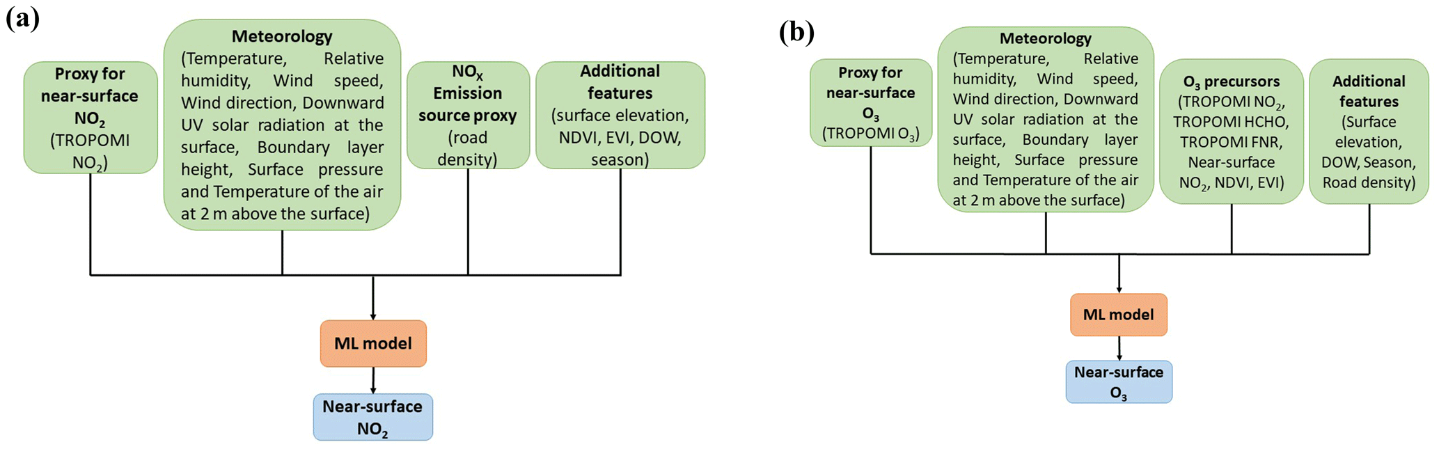
We primarily used the gradient-boosted tree (GBT) machine learning algorithm, XGBoost (Chen and Guestrin, 2016), to model near-surface NO₂ and O₃ concentrations. The GBT algorithm is a gradient-boosted decision-tree-based algorithm that is expected to outperform deep-neural-network-based algorithms for structured data (Lundberg et al., 2020). Furthermore, tree-based models are more interpretable and require less time to train than deep neural network algorithms. However, for comparison, we also used the multi-layer perceptron (MLP; neural network) algorithm (Gardner and Dorling, 1998). The GBT and MLP algorithms were implemented using scikit-learn, a Python module (https://scikit-learn.org/stable/, last access: 10 March 2023). When training the MLP model, we normalized the discrete feature variables between 0 and 1. The corresponding predictor variables and data flow for the NO₂ and O₃ ML model is shown in Fig. 2.

Figure 2 Predictor variables and data flow for the NO₂ (a) and O₃ (b) ML model.

To evaluate the ML model, we used the R² (coefficient of determination) and RMSE (root mean square error) metrics. We split the available data into training (70 % of the data) and testing (the remaining 30 %). The training data set was used to iteratively vary the hyperparameters (combinations) and select the best set of hyperparameters using a 5-fold CV (cross-validation). The hyperparameters used in this study are shown in Tables A2 and A3. We also evaluated the ML model using three different 5-fold CV testing strategies (random 5-fold CV, time-leave-out 5-fold CV, and location-leave-out 5-fold CV) with 100 % of the data (Meyer et al., 2018). In the random 5-fold CV testing strategy, the data were randomly split into five parts, four of which were used for training and one for testing. This procedure was repeated until all five parts had been used as test. The mean (and standard deviation) of R² and RMSE from the 5-fold CV were then computed. In the time-leave-out 5-fold CV testing strategy, the 5-fold CV procedure was the same, but the data were split based on time period (by date; i.e., from the start of study period to the end of study period). Similarly, in the location-leave-out 5-fold CV testing strategy, the data were split based on location (by latitude). Figure A1 shows the first 1-fold step in a 5-fold CV for time-leave-out and location-leave-out testing strategies. To interpret the importance of feature variables in the fitted model, we use SHAP (SHapley Additive exPlanations) values. The SHAP method (https://christophm.github.io/interpretable-ml-book/shap.html, last access: 10 March 2023) is the most commonly used method for interpreting ML model output, which calculates the contribution of each feature variable to the final prediction. Thus, higher SHAP values indicate greater feature importance.

2.5 CAMS model data

We obtained near-surface NO₂ and O₃ air quality forecasts from CAMS in order to compare the performance of our ML model to that of the chemical transport model. This data set is based on a data assimilation technique that combines real-time measurements with an ensemble of 11 air quality models to provide air quality data with high spatial resolution (0.1^∘) and 1 h temporal resolution over Europe; however, it is only available for 3 years in the rolling archive. We used data from 17 July 2019 to 31 January 2020. We did not use data after 31 January 2020 due to COVID-19 lockdown restrictions, during which many anthropogenic emission activities were limited, and CAMS had not adjusted the emission inventory for changes in emissions. This is because NO₂ has a short lifetime, so the effect of assimilated observations is minimal, and the CAMS-forecasted NO₂ product mostly reflects emissions prescribed in the inventory (Inness et al., 2015).

2.6 GEOS-Chem model data

In this study, GEOS-Chem (Goddard Earth Observing System with Chemistry; hereafter GC) chemical transport model simulations were used to normalize the meteorology effects when estimating the influence of the COVID-19 lockdown restrictions on air pollutant concentration changes. The GC simulations over the study area were obtained with a spatial resolution of $\mathrm{0.5}{}^{\circ }\times \mathrm{0.625}{}^{\circ }$ and 1 h temporal resolution for the 2020 strict COVID-19 lockdown period (21 March to 31 May) and the same period in 2019. Identical anthropogenic emissions from the 2014 Community Emissions Data System (CEDS) inventory were used for both 2020 and 2019 but with the corresponding meteorology, natural, and fire emissions in the respective years. Therefore, the difference in GC-simulated species (X) concentrations between 2020 and 2019 results from changes in meteorology, natural, and fire emissions between 2020 and 2019 (GC X_2020–2019); here, X refers to either NO₂ or O₃. Then, we subtracted the GC X_2020–2019 from the observed near-surface X_2020–2019 to estimate the changes in the concentrations of species X due to changes in anthropogenic emissions in the 2020 lockdown period (refer to the studies of Balamurugan et al., 2021; Qu et al., 2021, for detailed descriptions of the method).

3 Results

3.1 ML model evaluation and feature importance

The trained GBT model with 70 % of the data (78 433) for NO₂ reproduced the observed NO₂ concentration well in the test case (33615), with an R² of 0.88 and RMSE of 4.77 µg m⁻³ (Fig. 3a and Table 2). The random 5-fold CV results were in the same range ($R^{\mathrm{2}}=\mathrm{0.89}\pm \mathrm{0.002}$ and $\text{RMSE}=\mathrm{4.65}\pm \mathrm{0.034}$ µg m⁻³). The other two testing strategies (time-leave-out 5-fold CV and location-leave-out 5-fold CV) showed slightly worse agreement (Table 2), indicating that different validation strategies should be performed to interpret the ML model capability. Otherwise, it may result in an overoptimistic view of ML models (Meyer et al., 2018). Furthermore, the worse agreement in the location-leave-out 5-fold CV testing strategy suggests that there is less confidence in modeling the near-surface NO₂ over new locations that the GBT model has not been trained on before. However, these results outperformed the MLP model trained by another study (Chan et al., 2021; R=0.8 and RMSE=6.32 µg m⁻³ obtained for the testing strategy of the random split of 90 % of the data used for training and 10 % of the data used for testing) for near-surface NO₂ over Germany. Feature importance, based on the SHAP values, indicates that road density is the most important feature in the fitted model for NO₂ (Fig. 3c) because traffic is the main source of near-surface NO_x in urban areas. The next most important features were TROPOMI NO₂, boundary layer height, and elevation. Because the majority of NO_x sources are present at the surface, tropospheric column NO₂ data play an important role in explaining near-surface NO₂. Near-surface NO₂ typically has a negative correlation with the boundary layer height, as an increasing BLH disperses more, and vice versa (Balamurugan et al., 2021). Therefore, BLH is one of the most important features. It is unexpected that elevation was an important feature. The cause could be that the surface elevation varies greatly across Germany, influencing the total tropospheric column of NO₂ and thus serving as a link between the tropospheric column of NO₂ and near-surface NO₂. A previous study (Chan et al., 2021) also found that elevation was an important feature in the fitted MLP model for near-surface NO₂ over Germany.

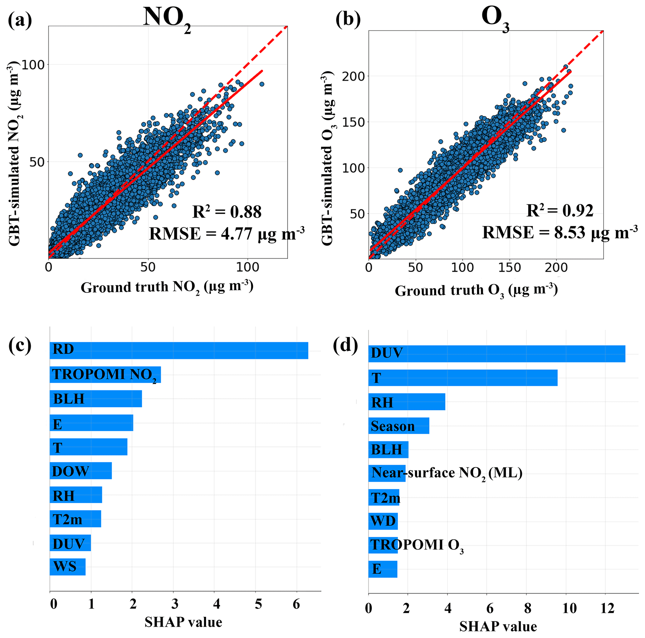
Figure 3 Comparison between the ground truth and GBT-simulated near-surface NO₂ (a) and O₃ (b). The feature importance (top 10) is calculated based on SHAP (SHapley Additive exPlanations) values for NO₂ (c) and O₃ (d) in the GBT model. RD is for road density, BLH is for boundary layer height, E is for surface elevation, T is for temperature, DOW is for day of the week, RH is for relative humidity, T_2 m is for temperature at 2 m height, DUV is for downwind UV radiation, WS is for wind speed, and WD is for wind direction.

Table 2 Evaluation metrics of our GBT model in different testing strategies.

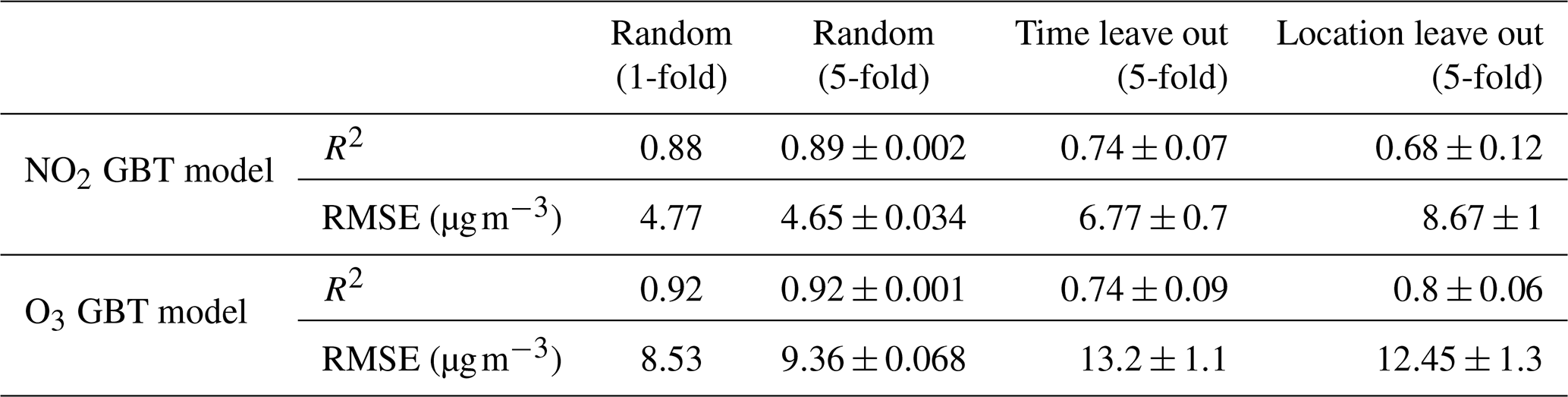
The GBT model trained with 70 % of the data (65 705) for O₃ also had a good representation of the observed O₃ concentrations in the test case (28 160), with an R² of 0.92 and RMSE of 8.53 µg m⁻³ (Fig. 3b). Similar to the NO₂ GBT model findings, time-leave-out 5-fold CV and location-leave-out 5-fold CV testing strategies showed less agreement than the random 5-fold CV testing strategy (Table 2). In comparison to our NO₂ GBT model, our O₃ GBT model demonstrated greater confidence in modeling near-surface O₃ over locations that the model was not trained on. According to SHAP values, the five most important features were DUV, T, RH, BLH, and season, with DUV having the greatest influence (Fig. 3d). Because ozone is formed in the atmosphere from the photolysis of NO₂, DUV plays a significant role in the fitted model that explains near-surface O₃. Temperature is the second most important feature, which is also not surprising, as it drives biogenic VOC emissions (an important precursor to O₃). Previous studies also show similar findings (Diao et al., 2021; Hu et al., 2021). GBT-modeled near-surface NO₂ was the sixth most important feature in the fitted model, according to the SHAP values, and it was also more important than TROPOMI NO₂.

Figure A2 shows the results obtained from the MLP model. Both the NO₂ and O₃ MLP models performed worse than the NO₂ and O₃ GBT models, respectively (Table A4 vs. Table 2). In particular, the MLP model findings showed poorer agreement in the time-leave-out 5-fold CV and location-leave-out 5-fold CV testing strategies. This supports previous studies (Heaton, 2020; Lundberg et al., 2020) and shows that the MLP model is unlikely to outperform tree-based models for tabular data. Because the GBT model outperforms the MLP model, we only considered the GBT model results in the following.

It is important to note that deep learning models are data intensive, and their performance and generalization capabilities tend to improve with larger amounts of data. In our study, we utilized the simplest deep learning algorithm known as MLP. However, it is essential to explore the capabilities of other deep learning algorithms, such as the CNN (convolutional neural network) and LSTM (long short-term memory), in future studies to gain further insight. Additionally, employing multiple ML models through bagging techniques could potentially lead to improved performance, despite the computational expense involved (He et al., 2022).

3.2 GBT model performance compared to CAMS

To evaluate how well our GBT model performs compared to CAMS, we compared the high-resolution near-surface NO₂ and O₃ forecasts from CAMS with observations and GBT-simulated near-surface NO₂ and O₃ with observations for the period between 17 July 2019 and 31 January 2020 (i.e., CAMS comparison period; Fig. 4). Please note this time period was not used for training the GBT model for this comparison. Our NO₂ GBT model reproduced the observed near-surface NO₂ concentrations well during this comparison period, with an R² of 0.82 and RMSE of 5.76 µg m⁻³, while CAMS NO₂ forecasts showed poor representation (R²=0.37 and RMSE=14.96 µg m⁻³). However, CAMS O₃ forecasts agreed slightly better with the observed concentrations (R²=0.93 and RMSE of 9.2 µg m⁻³) when compared to our O₃ GBT model (R²=0.85 and RMSE=13 µg m⁻³). Our NO₂ GBT model outperforms CAMS due to the fact that the effect of the data assimilation on the CAMS NO₂ forecast product is minimal, with CAMS simulations mostly reflecting the emissions provided in the inventory. Additionally, it should be noted that our GBT model requires less computational effort than the CAMS model.

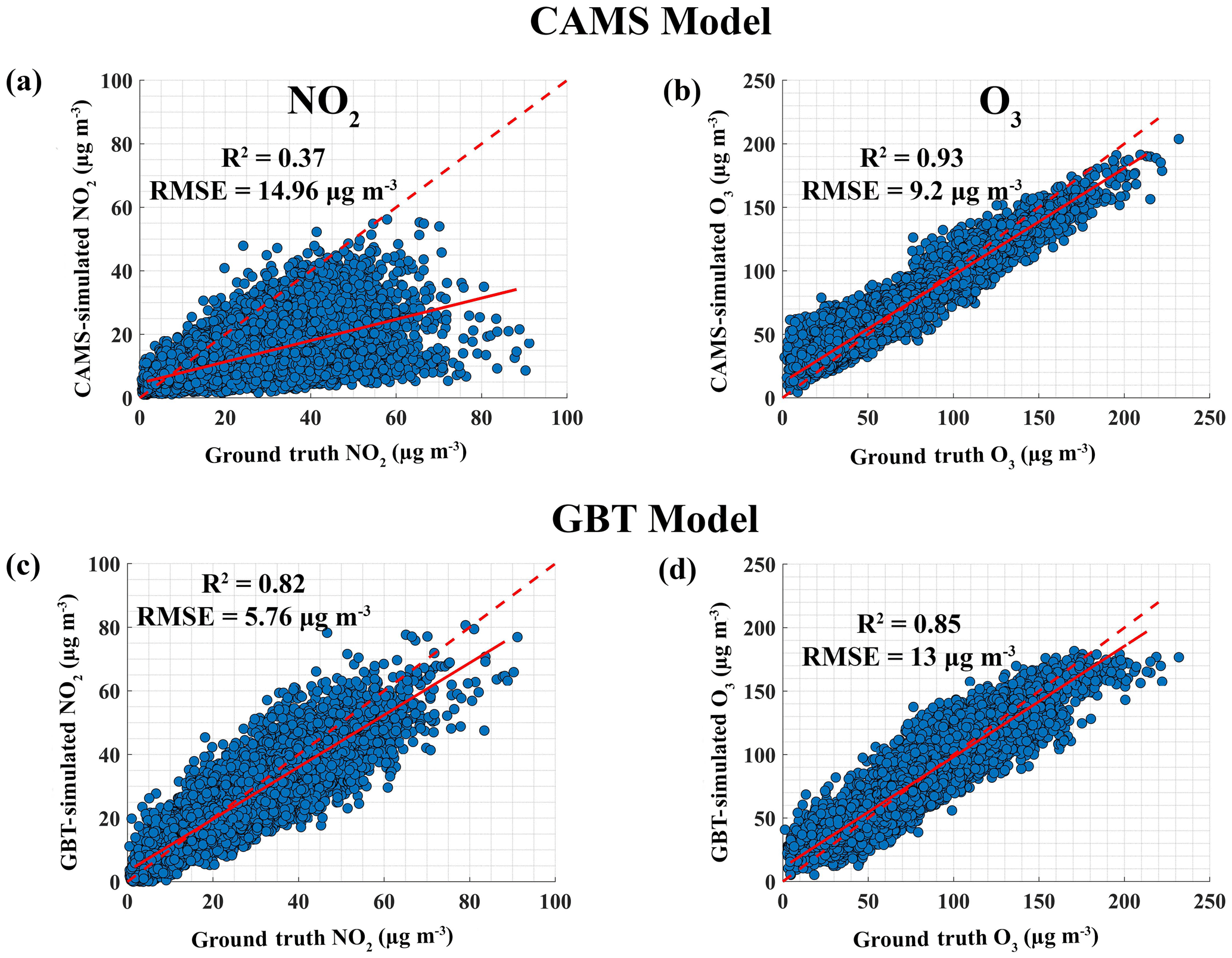
Figure 4 The top panels show the comparison between ground truth near-surface NO₂ and CAMS forecasts of near-surface NO₂ (a) and O₃ (b) for the period between 17 July 2019 and 31 January 2020. The bottom panels show the comparison between ground truth near-surface NO₂ and GBT-simulated near-surface NO₂ (c) and O₃ (d) values for the period between 17 July 2019 and 31 January 2020. The dotted line represents a 1:1 line, while the solid line represents a linear fit.

3.3 Spatiotemporal changes in near-surface NO₂ and O₃ over the study domain

After the discussed model evaluation, we trained the GBT model using 100 % of the data and modeled the near-surface NO₂ and O₃ concentrations over the study domain at 0.1^∘ resolution and daily (24 h mean for NO₂ and 8 h maximum mean for O₃) intervals. The averaged GBT-modeled near-surface NO₂ concentrations over the study domain during the study period are shown in Fig. 5a. The spatial variability in the near-surface NO₂ correlates with Germany's population density, and the main hotspots correspond to Germany's major metropolitan areas (Fig. A3). The study domain's main hotspot is western Germany (North Rhine-Westphalia; a federal state of Germany), which is Germany's industrial heartland. The number of days (%) that exceeded the 2021 World Health Organization (WHO) NO₂ limit ($\mathrm{24}\mathrm{h}\text{mean}>\mathrm{25}\mathrm{\mu }\mathrm{g}{\mathrm{m}}^{-\mathrm{3}}$) over major metropolitan areas in Germany was more than 50 %, with western Germany (North Rhine-Westphalia) experiencing the most days of exceedance during the study period (Fig. 7). Around 36 % of people live in locations where more than 25 % of the days exceed the WHO NO₂ limit during the study period (Fig. 8). The GBT-simulated near-surface O₃ showed a distinct spatial variability compared to NO₂, with high O₃ concentrations over southern Germany and low O₃ concentrations over northern Germany (Fig. 6). This could be due to the fact that O₃ is a secondary pollutant that is primarily driven by photochemical reactions influenced by meteorology, DUV, and temperature values, which were the factors with the most influence on photochemical reactions; accordingly, the most important features fitted in the O₃ GBT model were higher in southern Germany than northern Germany (Fig. A4). During the study period, more than 50 % of the study days in southern Germany exceeded the 2021 WHO O₃ limit (maximum $\mathrm{8}\mathrm{h}\text{mean}>\mathrm{100}\mathrm{\mu }\mathrm{g}{\mathrm{m}}^{-\mathrm{3}}$). Nearly 90 % of people live in locations where more than 25 % of the study days exceed the WHO O₃ limit (Fig. 8). Another interesting fact is that southern metropolitan areas and high NO_x regions have fewer days that exceeded the WHO O₃ limit than southern rural regions (Fig. 7). It is a well-known fact that rural regions have higher ozone levels than urban regions (Malashock et al., 2022). It could be because NO is a significant O₃ scavenger in higher NO_x (NO₂ is a proxy for NO_x) regions or because NO is in a NO_x-saturated regime. Furthermore, it is due to the fact that rural regions are the downwind locations of emission plumes and are the primary source of biogenic VOC emissions (Zong et al., 2018).

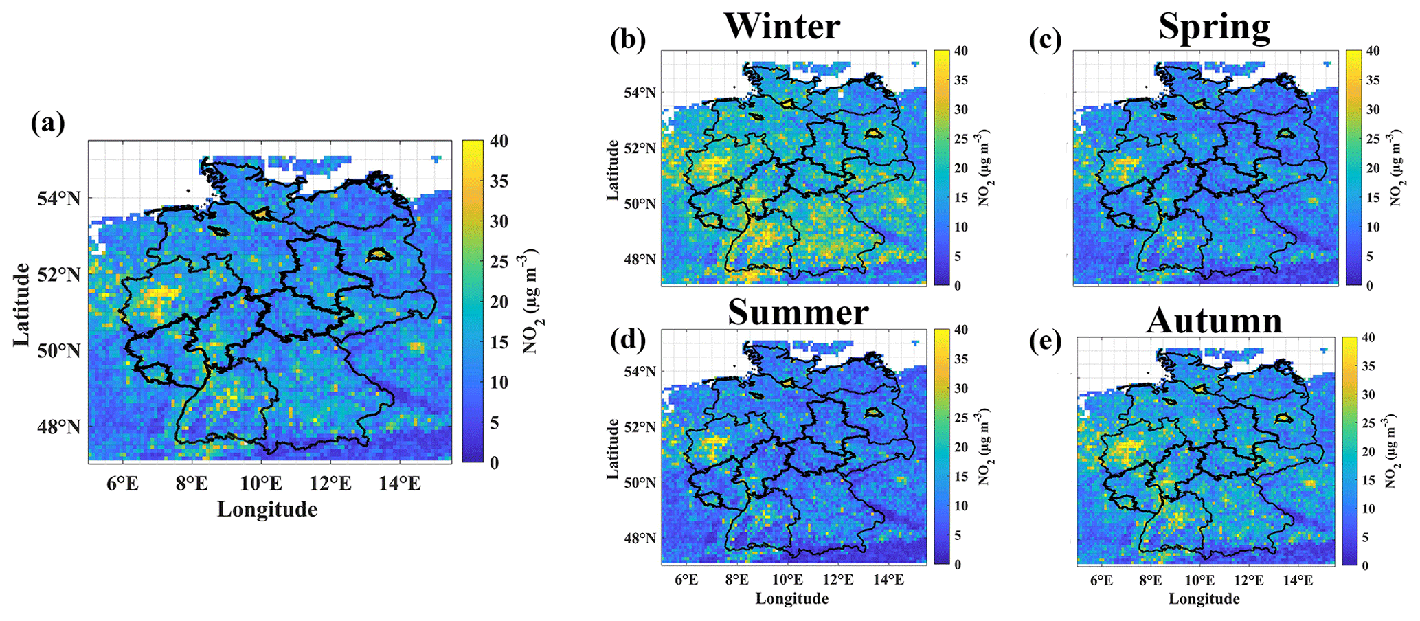
Figure 5 (a) Averaged GBT-simulated daily near-surface NO₂ concentrations over the study domain for the study period between 30 April 2018 and 1 July 2021. (b–e) Averaged GBT-simulated daily near-surface NO₂ concentrations for each season during the study period. Winter comprises the months of December, January, and February. Spring comprises the months of March, April, and May. Summer comprises the months of June, July, and August. Autumn comprises the months of September, October, and November.

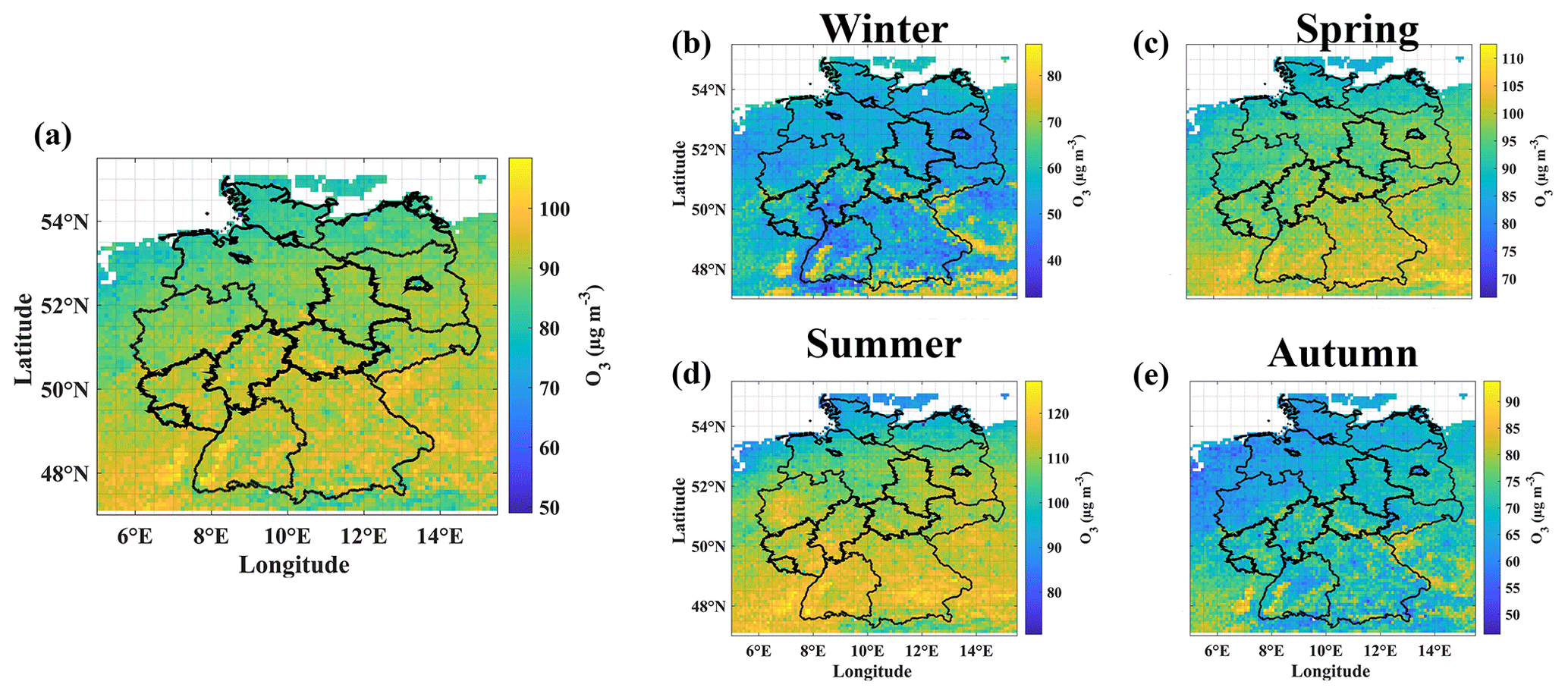
Figure 6 (a) Averaged GBT-simulated daily near-surface O₃ concentrations over the study domain for the study period between 30 April 2018 and 1 July 2021. (b–e) Averaged GBT-simulated daily near-surface O₃ concentrations for each season during the study period. Winter comprises the months of December, January, and February. Spring comprises the months of March, April, and May. Summer comprises the months of June, July, and August. Autumn comprises the months of September, October, and November.

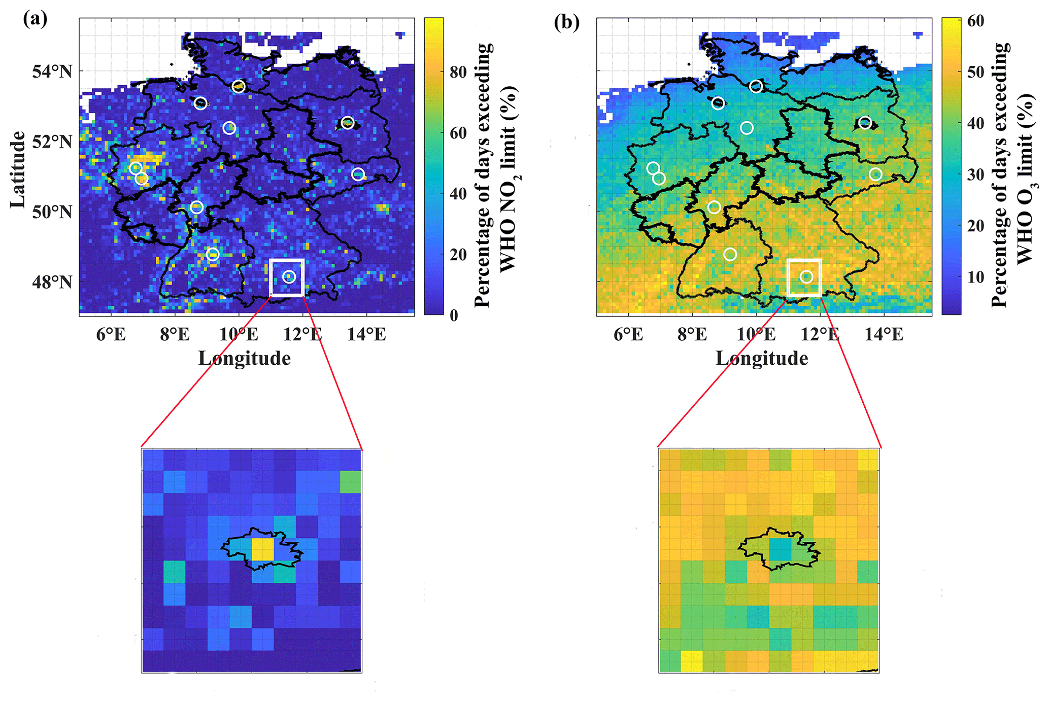
Figure 7 Number of days (%) that exceeded the WHO 24 h mean NO₂ (a) and maximum 8 h mean O₃ (b) limits over the study domain during the study period based on GBT model simulations. White circles represent major metropolitan areas. The metropolitan area of Munich and its surroundings (rectangular box) are enlarged to illustrate the urban vs. rural gradient. The administrative boundaries of Munich are marked in black in the insets.

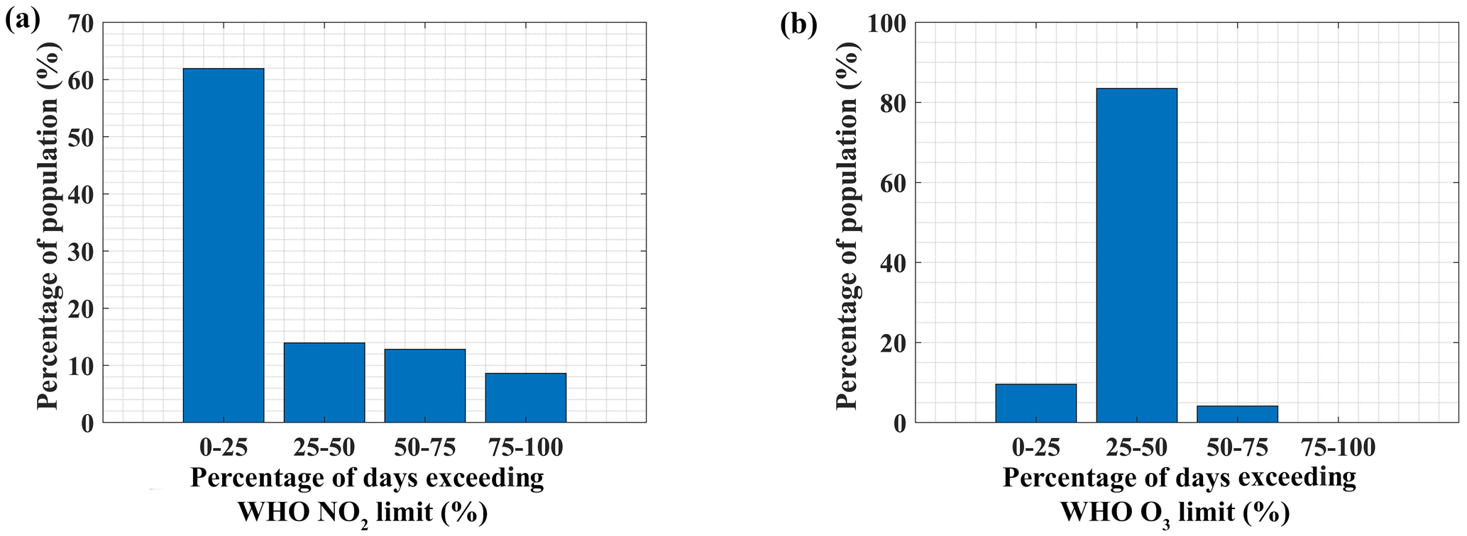
Figure 8 The population distribution in terms of the number of days (%) that exceeded the WHO 24 h mean NO₂ (a) and maximum 8 h mean O₃ (b) limits over the study domain during the study period based on GBT model simulations.

We also evaluated the model's capability to capture the exceedance events (above the WHO limit) using time-leave-out evaluation strategy. The exceedances of NO₂ and O₃ events simulated by the GBT model were compared with ground truth events in each iteration. This allows us to assess the model's ability to reproduce the exceedance events that have not been used in the training process. In total, 82 % of the WHO NO₂ and O₃ exceedance events in the whole data set (ground truth) were correctly identified as WHO NO₂ and O₃ exceedance events (true positives) in both the NO₂ and O₃ GBT models (Table A5). This indicates that our GBT model might slightly underestimates the exceedance events for both NO₂ and O₃. It could be due to unknown drivers that are not included in the model. However, we also noted that 6.6 % and 7.3 % of the data were incorrectly identified as exceedance events (false positives) by our NO₂ and O₃ GBT models, respectively.

The GBT-simulated near-surface NO₂ showed seasonal variations, as expected, with higher values in the winter season (Fig. 5). This is because of the high residential heating demand and favorable meteorology (e.g., a low boundary layer height) for pollutant accumulation and less NO₂ photolysis due to low solar radiation in the winter. The near-surface NO₂ hotspots were the same in all seasons, as seen in the overall study period average. In contrast, near-surface O₃ showed strong seasonal variations, with high values in the spring and summer due to high solar radiation (Fig. 6). It is worth noting that, as seen in the overall study period average, O₃ values in southern Germany were significantly higher in spring and summer than in northern Germany. Because near-surface O₃ is mainly driven by meteorology (DUV and temperature, which drive photochemical reactions and precursor emissions), the spatiotemporal variability is attributed to changes in meteorology. We also compared the spatial variability in the GBT-simulated near-surface NO₂ and O₃ to the CAMS forecasts product for the period between 17 July 2019 and 31 January 2020 (Figs. A5 and A6). The spatial variability in the GBT-simulated near-surface NO₂ and O₃ agreed well with the CAMS model. This implies that the ML model can supplement or replace the computationally expensive chemical transport models.

3.4 Influence of COVID-19 lockdown restrictions on near-surface NO₂ and O₃ changes

Due to the COVID-19 outbreak, many nations, including Germany, announced a lockdown in the spring of 2020. During that time period, various anthropogenic emission activities were restricted, particularly affecting traffic-related emissions. To estimate the influence of the lockdown restrictions on air pollutant concentration changes, we compared the GBT-simulated 2020 lockdown concentration with the same period in 2019. The 2020 lockdown period measurements were not used for GBT model training in this comparison. This can also be regarded as the critical performance evaluation of the GBT model.

When comparing different time periods, it is crucial to normalize the meteorology effects when estimating the impact of anthropogenic emission reductions (i.e., lockdown effects) on changes in air pollutant concentrations. Therefore, as described in Sect. 2, we used GC simulations to normalize the meteorology effects from GBT-simulated concentrations. After normalizing the meteorology effects, it is noticeable that high near-surface NO₂ levels decreased primarily over the previously observed hotspots (Fig. 9). The near-surface O₃ increased over western Germany, while decreasing elsewhere, particularly over low NO_x regions. We already observed that western Germany was a NO_x hotspot, possibly due to being a NO_x-saturated regime, so a reduction in NO_x increases ozone. Also, we could see that changes in near-surface O₃ were either negligible or slightly increased over metropolitan areas. The meteorology-normalized mean lockdown near-surface NO₂ decreased by about 23 % (± 5.3 %), while the meteorology-normalized mean lockdown near-surface O₃ increased by 1 % (± 4.6 %), over 10 major metropolitan areas (Berlin, Bremen, Cologne, Dresden, Düsseldorf, Frankfurt, Hamburg, Hanover, Munich, and Stuttgart) when compared to 2019. It increased by about 9 % in the Cologne and Düsseldorf metropolitan areas (located in western Germany) and slightly increased or decreased (between −3 % and +2 %) in other metropolitan areas when compared to 2019. This finding is consistent with other studies that found a decrease in the meteorology-normalized lockdown near-surface NO₂ and the small increase in the lockdown near-surface O₃ over German metropolitan areas when compared to 2019, using in situ measurements (Balamurugan et al., 2021, 2022b). We also evaluated our GBT model's ability to represent different emission scenarios by comparing weekends and weekdays; typically, anthropogenic NO_x emissions on weekends are lower than on weekdays due to reduced vehicle transportation. Our GBT model was also able to distinguish between the weekend and weekday emission scenarios; weekend near-surface NO₂ was lower than weekday near-surface NO₂, and as expected, there were no or only slight changes in weekend near-surface O₃ when compared to weekdays, with slight increases particularly over metropolitan areas (Fig. A7).

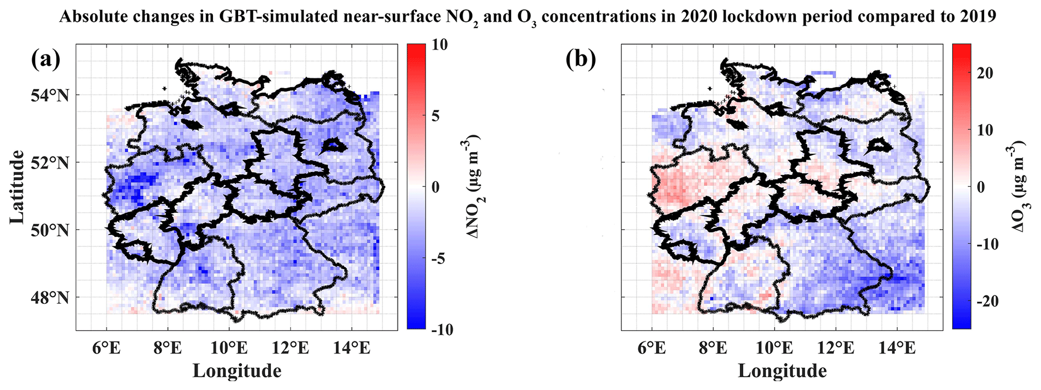
Figure 9 Absolute changes in GBT-simulated near-surface NO₂ and O₃ concentrations in 2020 lockdown period compared to the same period in 2019 after meteorology normalization.

3.5 Transferability of our GBT model

Although our study domain also covered parts of other European countries, we trained our GBT model using data from German measurement stations only. Therefore, comparing our trained GBT model simulations with measurements in other countries demonstrates how well our GBT model can model near-surface NO₂ and O₃ concentrations in neighboring parts of the world (similar to the location-leave-out testing strategy). We chose five major cities (Salzburg, Prague, Strasbourg, Liège, and Groningen) in different European countries covered by our study domain and compared their measured NO₂ and O₃ concentrations with GBT-modeled NO₂ and O₃ concentrations (Fig. 10 and Table A6).

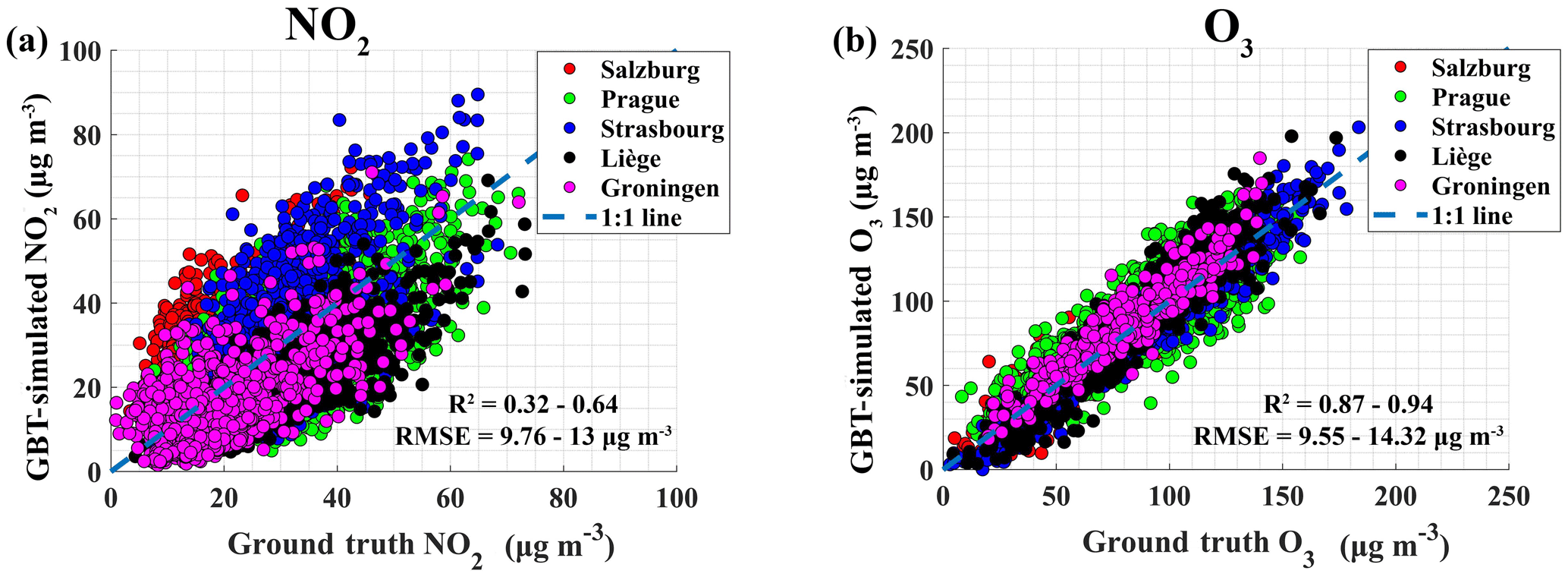
Figure 10 Comparison between ground truth and GBT-simulated near-surface NO₂ (a) and O₃ (b) for five different European metropolitan areas.

Our trained NO₂ GBT model based on German measurement stations explained 32 %–64 % (R² ranges between 0.32 and 0.64; RMSE ranges between 9.76 and 13 µg m⁻³) of the near-surface NO₂ measured in five metropolitan areas located outside of Germany, while the O₃ GBT model simulations agreed well with the observations (R² ranges between 0.87 and 0.94; RMSE ranges between 9.55 and 14.32 µg m⁻³). Since near-surface O₃ is mainly driven by meteorology, the O₃ GBT model trained using German measurement stations explains a large portion of near-surface O₃ in other locations. The worse agreement between the NO₂ GBT model predictions and NO₂ observations in other European countries suggests that information is lacking in the NO₂ GBT model to enable better representations of other locations, similar to location-leave-out 5-fold CV, which also showed poorer agreement for the NO₂ GBT model when modeling new locations (Table 2). Differences in the vehicle fleet composition and emission standards across different countries and locations would have an impact on our NO₂ GBT model predictions when applied to other countries or locations. In future work, other features and proxies besides road density could be considered to represent traffic emission.

4 Conclusion

This study simulated near-surface NO₂ and O₃ concentrations using an ML model over Germany at 0.1^∘ resolution and daily intervals. The ML model was used to link satellite column measurements (proxies for near-surface air pollutants), meteorology, and proxies for emission source information to near-surface NO₂ and O₃ concentrations. The ML models are extremely effective at learning the complex nonlinear relationships between variables. Therefore, in this study, we explored the capabilities of the ML models with respect to the spatiotemporal prediction of air pollutants. In addition, we investigated three aspects of the ML model, namely (1) how well our ML model performs compared to the chemical transport model, (2) how well our ML model can be used to assess the effectiveness of mitigation initiatives, and (3) how well our ML model can be transferred to locations where measurements are unavailable.

The following four different testing strategies were performed to evaluate the ML model's spatiotemporal predictions: (1) random split of data (70 % for training and 30 % for testing); (2) random 5-fold CV; (3) time-leave-out 5-fold CV; and (4) location-leave-out 5-fold CV. The gradient-boosted tree (GBT) model trained for NO₂ explained about 68 %–88 % of the observed NO₂ concentrations in Germany, with RMSE values of 4.77–8.67 µg m⁻³, whereas the GBT model trained for O₃ performed even better, with an R² of 0.74–0.92 and RMSE of 8.53–13.2 µg m⁻³. The evaluation metrics of the GBT model for different testing strategies differed significantly. This points out the importance of performing different testing strategies to interpret the true capability of the ML model. The road NO_x emission source proxy (road density) and TROPOMI tropospheric column NO₂ were the most important features in the fitted NO₂ GBT model. For O₃, the most important features were downward UV radiation at the surface and temperature. Since the multi-layer perceptron (MLP) model performed worse than the GBT model, the latter was used in further investigations in our study.

We also showed that our NO₂ GBT model outperforms the CAMS model, while slightly underperforming for near-surface O₃. The CAMS model forecast data set uses real-time observations with an ensemble of 11 air-quality models through data assimilation techniques, which are expected to be more computationally expensive than our GBT model. Therefore, the spatiotemporal variability in the near-surface NO₂ and O₃ concentrations and human exposure at a locations where no measurements are available can be studied with lower computational effort when using our GBT model. Near-surface NO₂ hotspots were found over German metropolitan areas, particularly in western Germany. The near-surface NO₂ hotspot locations did not change with the seasons but had high values in the winter. However, near-surface O₃ showed high seasonal variability, with high values in the spring and summer and no definite hotspots. Overall, southern Germany experiences higher ozone levels than northern Germany due to higher downward UV radiation and temperatures in southern Germany compared to northern Germany. Even though metropolitan areas were the NO₂ hotspots, rural regions, particularly in southern Germany, had higher O₃ concentrations than metropolitan areas. It is because rural areas are dominated by meteorology-driven biogenic VOC emissions and are generally situated downwind of the emission plume. About 36 % of people live in locations where the WHO NO₂ limit exceeds more than 25 % of the days during the study period. Meanwhile, 90 % of people live in areas where the WHO O₃ limit is exceeded for more than 25 % of the study days.

Our study also demonstrated the GBT model's capability to assess the efficacy of mitigation strategies. For example, our GBT model reproduced the observations that, during the 2020 COVID-19 lockdown period, meteorology-normalized near-surface NO₂ was significantly reduced, while meteorology-normalized near-surface O₃ was slightly increased or decreased over metropolitan and industrial areas over Germany when compared to 2019. These findings agreed with those of other studies that used in situ measurements.

Our GBT ML model's transferability is assessed by comparing simulations from our GBT model trained with measurements in Germany to measurements in other European countries. Our NO₂ GBT model showed moderate agreement with observations from other countries (R² ranges between 0.32 and 0.64, and RMSE ranges between 9.76 and 13 µg m⁻³), implying a lack of information in the GBT model when modeling near-surface NO₂ over other countries, which may have different vehicle fleet composition and emissions standards. However, our O₃ GBT model performed well (R² ranges between 0.87 and 0.94, and RMSE ranges between 9.55 and 14.32 µg m⁻³), indicating that our O₃ GBT model can be used to model the O₃ concentrations in other countries, at least in neighboring European countries.

Appendix A

Table A1 Different types of stations (%) considered in this study (based on locations specified by the European Environment Agency).

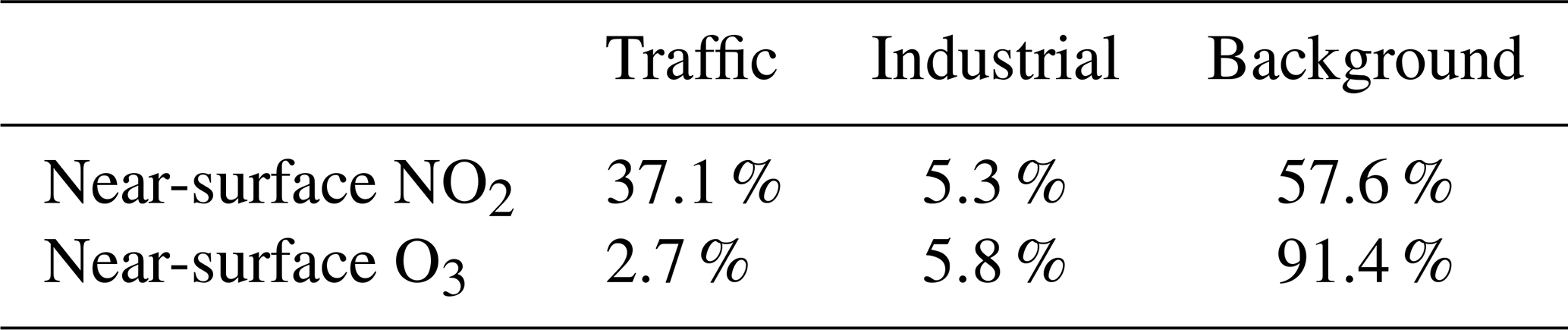
Table A2 The hyperparameters of the GBT model for each pollutant used in the study.

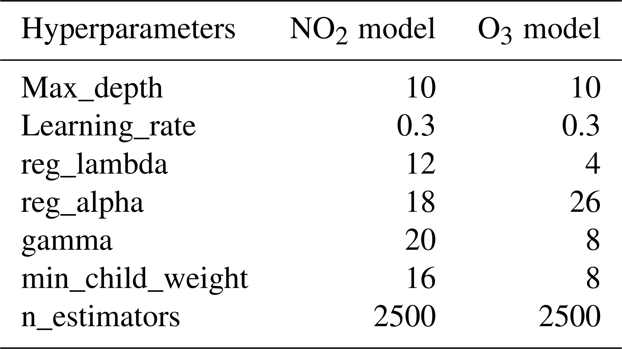
Table A3 The hyperparameters of the MLP model for each pollutant used in the study.

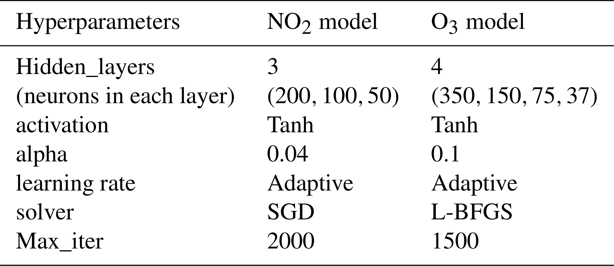
L-BFGS is the limited-memory Broyden–Fletcher–Goldfarb–Shanno. SGD is the stochastic gradient descent.

Table A4 Evaluation metrics of our MLP model in different testing strategies.

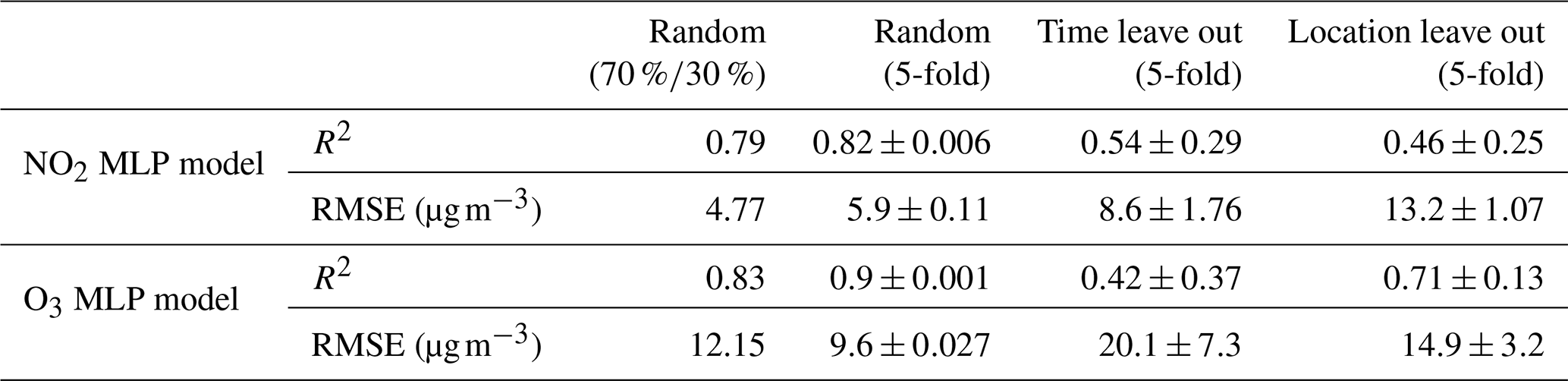
Table A5 Comparison between the WHO NO₂ and O₃ exceedance events in the ground truth data set and GBT-simulated WHO NO₂ and O₃ exceedance events using time-leave-out testing strategy.

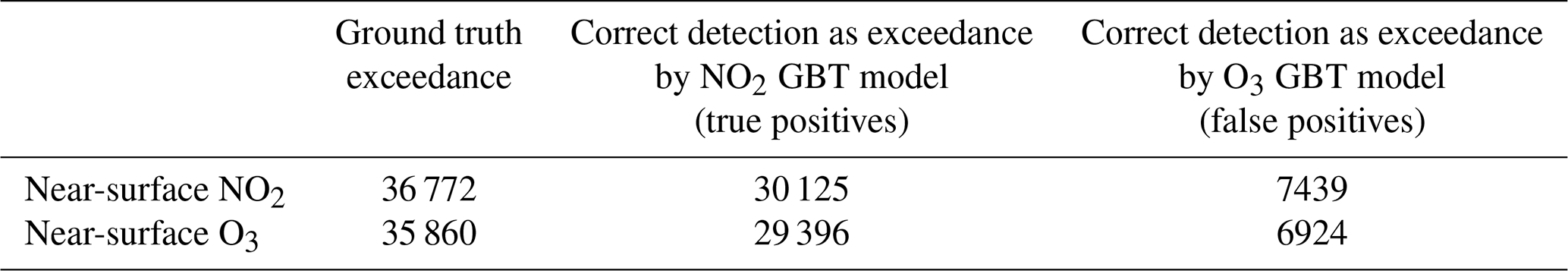
Table A6 Metropolitan areas in other European cities considered for the evaluation of GBT model. The evaluation metrics (comparison between GBT simulations and in situ measurements) for NO₂ and O₃ shown in last two columns for each city.

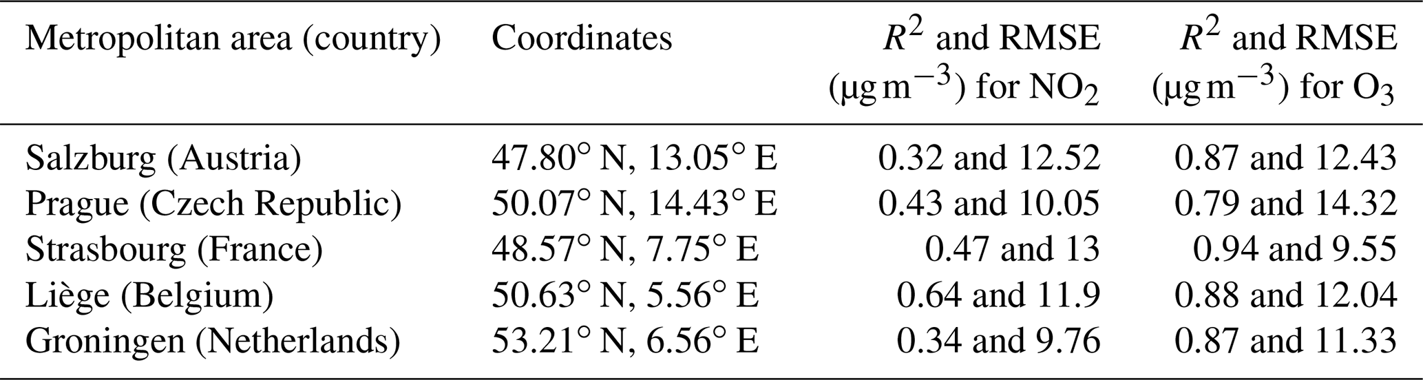
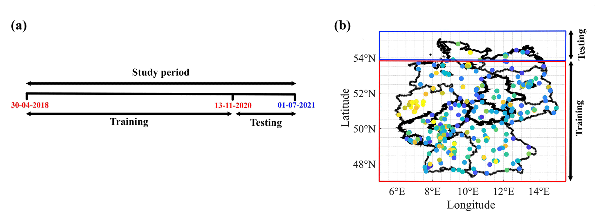
Figure A1 A first 1-fold step in 5-fold CV is illustrated for time-leave-out (a) and location-leave-out (b) testing strategies. In time-leave-out 5-fold CV, the data were divided into five parts based on the time period (date-wise), with four parts used for training and one part being tested. This process is repeated until each part (a total of five) has been tested. Similarly, in location-leave-out 5-fold CV, the data were divided into five parts based on location (latitude), with four parts used for training and one part being tested. This process is repeated until each part (a total of five) has been tested.

Figure A2 Comparison between ground truth and MLP-simulated near-surface NO₂ (a) and O₃ (b). The dotted line represents a 1:1 line, while the solid line represents a linear fit.

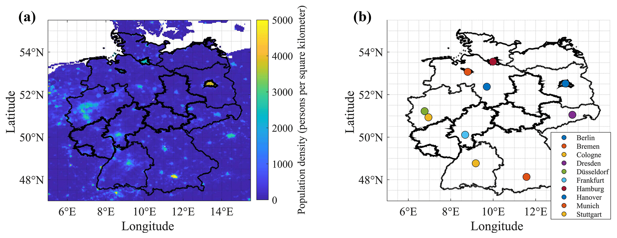
Figure A3 Population density for the year 2020 (a) and the locations of major German metropolitan areas (b).

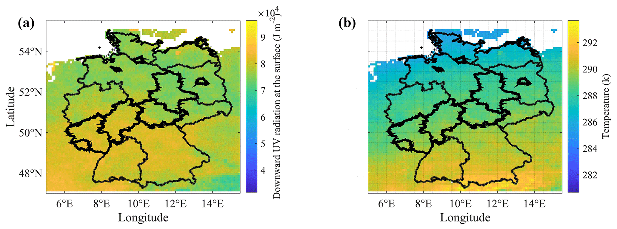
Figure A4 Averaged downward UV radiation at the surface (a) and temperature (b) over the study domain during the study period.

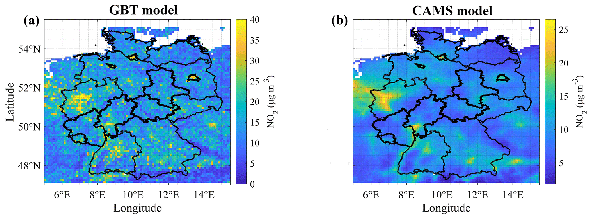
Figure A5 Averaged GBT-simulated near-surface NO₂ concentrations (a) and CAMS forecast near-surface NO₂ concentrations (b) over the study domain for the period between 17 July 2019 and 31 January 2020.

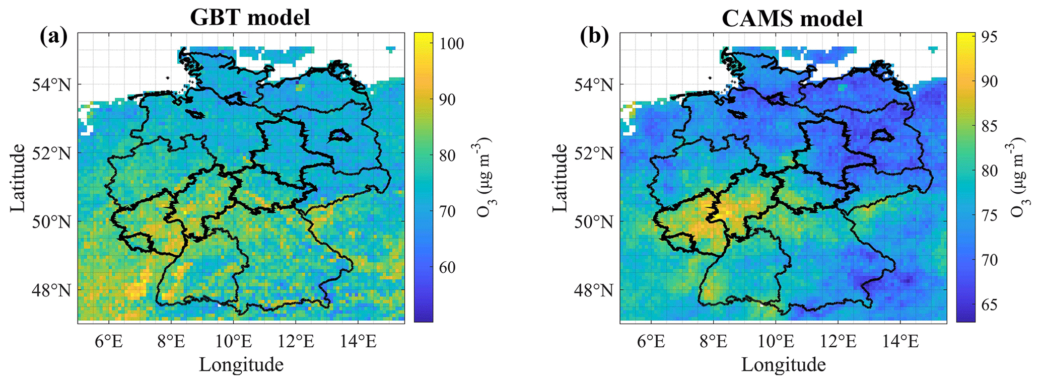
Figure A6 Averaged GBT-simulated near-surface O₃ concentrations (a) and CAMS forecast near-surface O₃ concentrations (b) over the study domain for the period between 17 July 2019 and 31 January 2020.

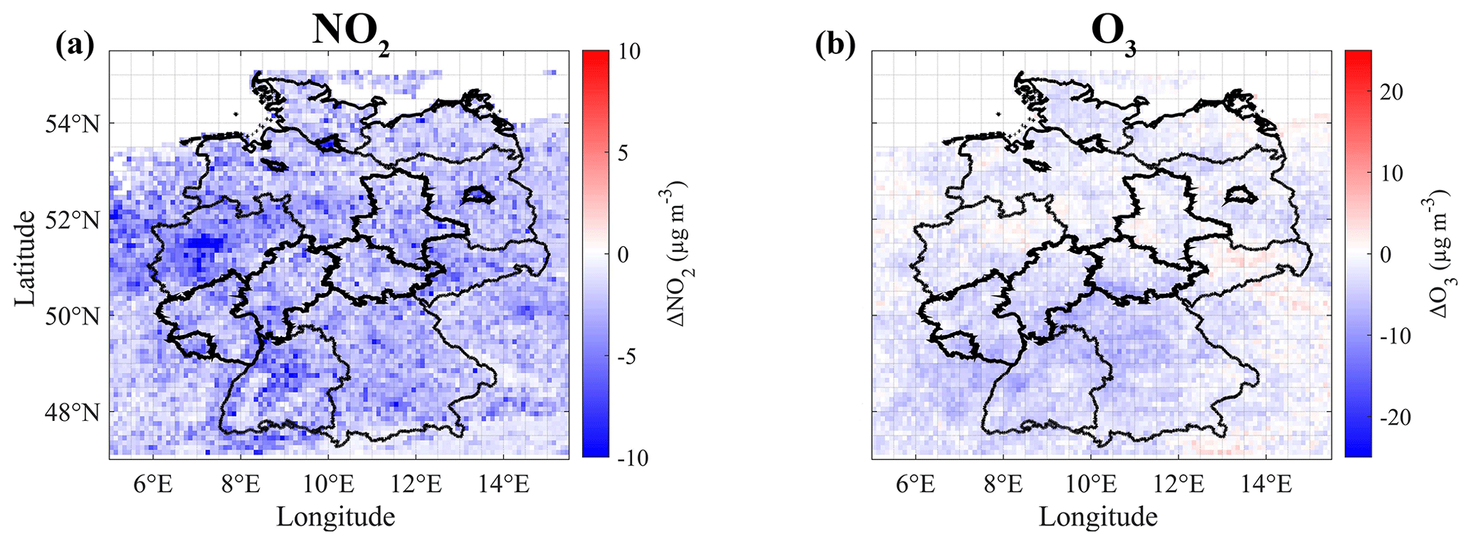
Figure A7 The difference in GBT-simulated near-surface NO₂ (a) and O₃ (b) concentrations between weekends and weekdays during the study period.