the Creative Commons Attribution 4.0 License.
the Creative Commons Attribution 4.0 License.
 | 04 Jan 2022
Dependency of the impacts of geoengineering on the stratospheric sulfur injection strategy – Part 1: Intercomparison of modal and sectional aerosol modules
Ulrike Niemeier
Daniele Visioni
Simone Tilmes
Harri Kokkola
Injecting sulfur dioxide into the stratosphere with the intent to create an artificial reflective aerosol layer is one of the most studied options for solar radiation management. Previous modelling studies have shown that stratospheric sulfur injections have the potential to compensate for the greenhouse-gas-induced warming at the global scale. However, there is significant diversity in the modelled radiative forcing from stratospheric aerosols depending on the model and on which strategy is used to inject sulfur into the stratosphere. Until now, it has not been clear how the evolution of the aerosols and their resulting radiative forcing depends on the aerosol microphysical scheme used – that is, if aerosols are represented by a modal or sectional distribution. Here, we have studied different spatio-temporal injection strategies with different injection magnitudes using the aerosol–climate model ECHAM-HAMMOZ with two aerosol microphysical modules: the sectional module SALSA (Sectional Aerosol module for Large Scale Applications) and the modal module M7. We found significant differences in the model responses depending on the aerosol microphysical module used. In a case where SO2 was injected continuously in the equatorial stratosphere, simulations with SALSA produced an 88 %–154 % higher all-sky net radiative forcing than simulations with M7 for injection rates from 1 to 100 Tg (S) yr−1. These large differences are identified to be caused by two main factors. First, the competition between nucleation and condensation: while injected sulfur tends to produce new particles at the expense of gaseous sulfuric acid condensing on pre-existing particles in the SALSA module, most of the gaseous sulfuric acid partitions to particles via condensation at the expense of new particle formation in the M7 module. Thus, the effective radii of stratospheric aerosols were 10 %–52 % larger in M7 than in SALSA, depending on the injection rate and strategy. Second, the treatment of the modal size distribution in M7 limits the growth of the accumulation mode which results in a local minimum in the aerosol number size distribution between the accumulation and coarse modes. This local minimum is in the size range where the scattering of solar radiation is most efficient. We also found that different spatial-temporal injection strategies have a significant impact on the magnitude and zonal distribution of radiative forcing. Based on simulations with various injection rates using SALSA, the most efficient studied injection strategy produced a 33 %–42 % radiative forcing compared with the least efficient strategy, whereas simulations with M7 showed an even larger difference of 48 %–116 %. Differences in zonal mean radiative forcing were even larger than that. We also show that a consequent stratospheric heating and its impact on the quasi-biennial oscillation depend on both the injection strategy and the aerosol microphysical model. Overall, these results highlight the crucial impact of aerosol microphysics on the physical properties of stratospheric aerosol which, in turn, causes significant uncertainties in estimating the climate impacts of stratospheric sulfur injections.
- Article
(8270 KB) - Full-text XML
- Companion paper
-
Supplement
(8024 KB) - BibTeX
- EndNote


Solar radiation management (SRM) techniques have been proposed to complement mitigation efforts to avoid greenhouse-gas-driven catastrophic global warming (e.g. Caldeira et al., 2013). These techniques might be considered if major reductions in greenhouse gas (GHG) emissions are not achieved or if the development of efficient carbon dioxide removal techniques are delayed. Instead of altering the increased GHG concentration in the atmosphere, which is suppressing outgoing long-wave (LW) radiation, SRM techniques would aim to reflect more short-wave (SW) radiation from the Earth's atmosphere back to space in order to mitigate GHG-induced changes in the net radiation flux. Even though SRM could, in theory, be used to mitigate or even compensate for the global mean net radiation flux changes due to GHGs, the SW and LW radiative fluxes would still be zonally and vertically different compared with those in the unperturbed atmosphere. This would lead to some side effects. For example, offsetting GHG-induced warming by reflecting more radiation would decrease the global mean precipitation (Tilmes et al., 2013; Laakso et al., 2020); this could lead to cooling of the tropics, whereas high latitudes would still be warmer than prior to GHG-induced warming if solar radiation was reduced uniformly (e.g. percent solar constant reduction) (Kravitz et al., 2021).
One of the most cost-efficient techniques to increase the reflectivity of the Earth is continuous stratospheric aerosol intervention (SAI) using sulfur. This technique mimics large volcanic eruptions, during which a large amount of sulfur reaches the stratosphere, subsequently producing aerosols from gaseous sulfur that form a long-lasting (1–2 years) reflective blanket and temporally cool the climate. Thus, this is one of the few, if not the only, SRM technique for which observational evidence exists supporting its efficiency in cooling the climate at a global scale. However, due to the rare occurrence of large volcanic eruptions that have long-lasting climate impacts, there are only good modern-day observations of volcanic aerosols properties and radiative effects for one large volcanic eruption, Mt. Pinatubo in 1991. In addition, sulfur from large volcanic eruptions is released into a relatively particle-free stratosphere. In the case of SAI, sulfur injections are instead done continuously onto an existing particle field from the preceding injections. This would affect the size distribution of the stratospheric aerosols and the following radiative and climate impacts. Hence, drawing conclusions on the possible impacts of SAI based on observations of large volcanic eruptions is not straightforward. Because of this non-linear nature of aerosol evolution and the lack of measurements after large volcanic eruptions, climate model simulations are required to understand climate impacts of SAI.
There are several approaches to model SAI. In some studies, the effect of stratospheric sulfur injections are imitated by decreasing the solar constant, although this is not a good proxy for the radiative impacts of stratospheric aerosols (Visioni et al., 2021). Aerosols absorb a part of the long-wave radiation that has an impact on the atmospheric energy budget and on atmospheric dynamics. In addition, the cooling potential and the spatial distribution of radiative forcing depend on aerosol microphysics and the transport of the particles. Studies in which the aerosol microphysics is simulated have shown that global mean radiative forcing does not increase linearly with the amount of sulfur injected (Heckendorn et al., 2009; Pierce et al., 2010; Niemeier et al., 2011). Increasing the magnitude of the injection leads to larger particles with a smaller number concentration. Larger particles work as an efficient condensation sink for gaseous sulfuric acid and a coagulation sink for new particles forming via nucleation. Tilmes et al. (2018a) showed a linear relationship between the injection amount and temperature reduction in SAI. However, this relation was defined based on scenarios in which the background conditions were not fixed and the injection strategy was changed during the simulation (see e.g. Visioni et al., 2020a); thus, these results are not directly comparable with the above-mentioned studies.
There is a large diversity in the predicted radiative forcing of SAI between studies in which aerosol microphysics is simulated. For example, based on Niemeier and Timmreck (2015), the injection rate of 10 Tg (S) yr−1 leads to a −(1.79–2.06) W m−2 all-sky radiative forcing at the top of the atmosphere (TOA). Based on Laakso et al. (2020), only 3 Tg (S) yr−1 was required to induce a radiative forcing of the same magnitude (−2.2 W m−2). Injecting 6 Tg (S) yr−1 in the study by Laakso et al. (2020) resulted in a −3.72 W m−2 total radiative forcing, whereas achieving the same cooling effect required 20 Tg (S) yr−1 in the simulations of Niemeier and Timmreck (2015). Both studies used a different generation of the same general circulation model (GCM) ECHAM, but the main difference was how the aerosol microphysical processes were modelled. Simulations by Niemeier and Timmreck (2015) were done with a modal aerosol model (M7), whereas a sectional model (SALSA; Sectional Aerosol module for Large Scale Applications) was used in Laakso et al. (2020).
In addition, Kleinschmitt et al. (2018) studied the dependency of geoengineering on the magnitude of SAI using a GCM with a sectional aerosol scheme (LMDZ-S3A). Their results on net radiative forcing where close to the values in Niemeier and Timmreck (2015), but both the LW and SW radiative forcing, which had opposite impacts on net radiation (i.e different signs), were individually significantly larger. In Niemeier and Timmreck (2015), the LW forcing efficiency (forcing per injected sulfur Tg (S) yr−1) was roughly 0.1 W m−2/(Tg (S) yr−1) regardless of injection rate. SW forcing efficiency was −0.35 with a 1 Tg (S) yr−1 sulfur injection rate and decreased gradually to −0.22 W m−2/(Tg (S) yr−1 when the injection rate was increased to 50 Tg (S)−1. In Kleinschmitt et al. (2018), the corresponding change in the SW forcing efficiency was −0.5 to −0.3 W m−2/(Tg (S) yr−1, whereas the LW forcing varied between 0.2 and 0.3 W m−2/(Tg (S) yr−1. Kravitz et al. (2017) simulated injections with strengths between 1 and 25 Tg (S) yr−1 with CESM1(WACCM), the Community Earth System Model (Whole Atmosphere Community Climate Model), where the aerosol size distribution is represented using three modes. In their study, the SW forcing efficiency varied roughly from −1.0 to −0.7 W m−2/(Tg (S) yr−1, and the LW forcing varied from 0.7 to 0.6 W m−2/(Tg (S) yr−1. However, these fluxes were calculated from fully coupled simulations and, thus, are not fully comparable to the direct radiative forcing estimates of the other above-mentioned studies.
In addition to the fact that the simulated radiative effects depend on which model is used, they also depend on the injection strategy and how injections are varied spatially and temporally. There is a good agreement between studies in that when injection rates are lower than 10 Tg (S) yr−1, increasing the altitude of the injection increases the lifetime of aerosols and the radiative forcing (Heckendorn et al., 2009; Niemeier et al., 2011; Kleinschmitt et al., 2018; Vattioni et al., 2019; Tilmes et al., 2018b); however, with higher injection rates, the inverse can be found, as shown by Niemeier and Schmidt (2017).
Most existing studies have simulated the impacts of injections over the Equator, where the yearly average solar intensity is highest. In addition, due to the Brewer–Dobson circulation, it takes longer for aerosol to be transported to high latitudes, where the sedimentation rate is higher than at low latitudes. Niemeier et al. (2011) showed that injecting into only one model grid box induced a stronger radiative forcing compared with scenarios in which injections were performed in a band over the Equator. However, based on Vattioni et al. (2019), injecting into one grid box or band over longitudes did not have a significant impact. In contrast, Mills et al. (2017) found that injections along one longitude result in larger particles than point injections and are, therefore, less efficient. English et al. (2012) showed that an injection into a broader band over the Equator increased the lifetime of sulfur, whereas Vattioni et al. (2019) did not find a significant impact of broadening the injection area. Kleinschmitt et al. (2018) also found that broadening the injection band had a negligible effect on the net radiative forcing, but the respective SW and LW forcing, which have inverse impacts on the radiation, decreased by 20 %–30 % in the case of a 10 Tg (S) yr−1 injection rate.
Sulfur can also be injected at a certain time of the year instead of continuous injections. Heckendorn et al. (2009) and Niemeier et al. (2011) studied scenarios in which injections were done twice a year. Based on Heckendorn et al. (2009), this strategy of using pulsed injections increased the forcing by more than 50 % compared with continuous injections. However, based on Niemeier et al. (2011), continuous and pulsed injection scenarios did not exhibit a large difference in their radiative impacts. Visioni et al. (2019) simulated single-point injections at different latitudes in certain seasons and showed that this can reduce the sulfur required to achieve a certain aerosol optical depth. The injection area can also be varied spatially depending on the season. Laakso et al. (2017) and Kleinschmitt et al. (2018) showed that this led to a slight increase in radiative forcing compared with continuous equatorial injections, but the zonal distribution of the forcing was concentrated relatively more on mid-latitudes and less over the tropics. The sensitivity of the modelled response to different spatio-temporal injection strategies can also be dependent on the injection magnitude, which has not been studied to date.
Overall, as the studies listed above show, there is a large diversity in radiative forcings for SAI between studies, and the differences depend on which general circulation model and microphysical module are used, how the injections are varied spatially and temporally, and the magnitude of the sulfur injections. Simulating aerosol microphysics is computationally expensive. This sets limitations on the investigation of different injection scenarios with different amounts of sulfur injected. However, increases in computing capacity over the last few years have enabled the study of a wide range of different injection strategies within a feasible computation time. There are only few aerosol–climate models that include both modal and sectional approaches for representing the aerosol size distribution and calculating aerosol microphysics which would allow one to study how the aerosol microphysics scheme affects the simulated impacts of SAI. Here, we carry out a comprehensive study on the radiative impacts of stratospheric sulfur injections. We use the ECHAM-HAMMOZ aerosol–climate model, which includes both the modal aerosol module M7 and the sectional aerosol module SALSA. These modules have shown stratospheric aerosol loads consistent with the observations of the Mt. Pinatubo 1991 eruption (Niemeier et al., 2009; Toohey et al., 2011; Laakso et al., 2016; Kokkola et al., 2018). Here, both modules are used to study how the simulated impacts of geoengineering depend on the injection strategy and injection magnitude as well as how these results depend on the aerosol microphysical module used.
2.1 The ECHAM-HAMMOZ aerosol–climate model
Simulations were done with the ECHAM-HAMMOZ (ECHAM6.3-HAM2.3-MOZ1.0) aerosol–climate model (Zhang et al., 2012; Kokkola et al., 2018; Schultz et al., 2018; Tegen et al., 2019). The host model is the ECHAM6.3 general circulation model (Stevens et al., 2013). Simulations were performed with a T63L95 resolution which corresponds to an approximately 1.9∘ × 1.9∘ horizontal grid. The atmosphere was divided into 95 vertical levels reaching up to 80 km. This resolution enables one to resolve the quasi-biennial oscillation (QBO) in the tropical stratosphere which has an impact on the transport of the stratospheric aerosols.
The HAM aerosol module is interactively coupled to ECHAM and its radiation module (Tegen et al., 2019). HAM calculates the emissions, removal, and radiative properties of the major global aerosol compounds of sulfate, organic carbon, black carbon, sea salt and mineral dust. It includes gas- and liquid-phase chemistry of sulfur. ECHAM-HAMMOZ also includes the chemistry model MOZART (Model for OZone And Related chemical Tracers). Using this model configuration would allow the online calculation of ozone and the hydroxyl radical (OH), which is the main oxidizing agent of SO2. However, this model configuration is computationally expensive: it would triple the computational time, and its impact on the stratospheric sulfur field was relatively small compared with the impact of microphysical processes in our test simulations (not shown). This is because continuous injection rates mean that only a fraction is injected each day; thus, stratospheric OH concentrations are not as depleted as in the case of large volcanic eruptions during which several megatons of sulfur is dumped during a few hours. However, as shown by Richter et al. (2017), SAI has a significant impact on the ozone concentration which, in turn, impacts the atmospheric dynamics and injected aerosols. Nevertheless, we did not include MOZART as an active component in our simulations, and OH and ozone concentrations were prescribed by a monthly mean climatology. The sea surface temperature, sea ice, and the atmospheric GHG concentration and aerosol emissions were fixed to the year 2005 levels. The aerosol surface emissions were based on the ACCMIP (Emissions for Atmospheric Chemistry and Climate Model Intercomparison Project) anthropogenic emission inventory. Emissions for sea salt and dust are calculated online.
In this study, the term “radiative forcing” refers to the instantaneous radiative forcing, which is calculated by a double radiation call with and without aerosols and as the difference between a specific SAI experiment and control simulation.
The microphysical processes of nucleation, condensation, coagulation and hydration were simulated by the microphysical module. For this, ECHAM-HAMMOZ has two options: SALSA, where aerosols are represented by size bins of fixed width, and M7, where aerosols are represented using log-normal modes. Both modules have been shown to simulate the stratospheric aerosol loads and radiative properties consistently compared to the observations of the Mt. Pinatubo 1991 eruption (Kokkola et al., 2018). However, when using M7, this requires changes in the configuration of the mode and a narrower width of the largest mode to improve the representation of the stratospheric aerosols (Kokkola et al., 2009). Thus, one downside of using a modal scheme is that tropospheric and stratospheric aerosols are not well described with the same model configuration.
2.1.1 Sectional aerosol module – SALSA
SALSA describes aerosols using 10 size bins in size space. The seven largest bins are represented separately for soluble and insoluble material. A detailed description of SALSA is given in Kokkola et al. (2018). SALSA bins are divided into subregions, where the first subregion covers the three smallest bins and the second subregion covers the other seven larger bins. The particle size distribution (i.e moving particles from one size bin to another) is updated (at each time step) based on the mean volume of the bin, assuming that aerosols in the bin are evenly distributed, and on the actual mean volume of the particle population (calculated based on the mass and number of aerosols) in the corresponding bin, after the microphysical processes have been calculated. If the actual mean volume of the particle population is larger than the mean volume of the monodisperse size bin, a certain part of the aerosol population is moved to the next bin. This method is called hybrid bin (Young, 1974; Chen and Lamb, 1994). The scheme for new particle formation is based on the Kerminen and Kulmala (2002) J3 parametrization, which produces aerosols with a diameter of 3 nm. A 3 nm diameter is also the lowest bound for the SALSA size distribution in the standard set-up. Thus, the produced 3 nm particles are smaller than the volume mean diameter of the smallest bin in the default configuration. If new particle formation is efficient, the produced 3 nm particles might keep the actual mean diameter of the smallest bin low. This prevents particles in the bin from being moved to the next bin. This led to an very high number concentration in the smallest bin in our first preliminary simulations. This was solved by changing the lower bound the size range of the first subregion (three smallest bins) from 3 to 1.02873 nm so that the volume mean diameter of smallest bin was the same as the diameter of the newly formed particles (3 nm). This led to a smaller number concentration in the smallest size bin and a clearly higher concentration in second smallest bin. A change in the lower bound of the first subregion was the only change that was made to the default set-up in SALSA (Kokkola et al., 2018).
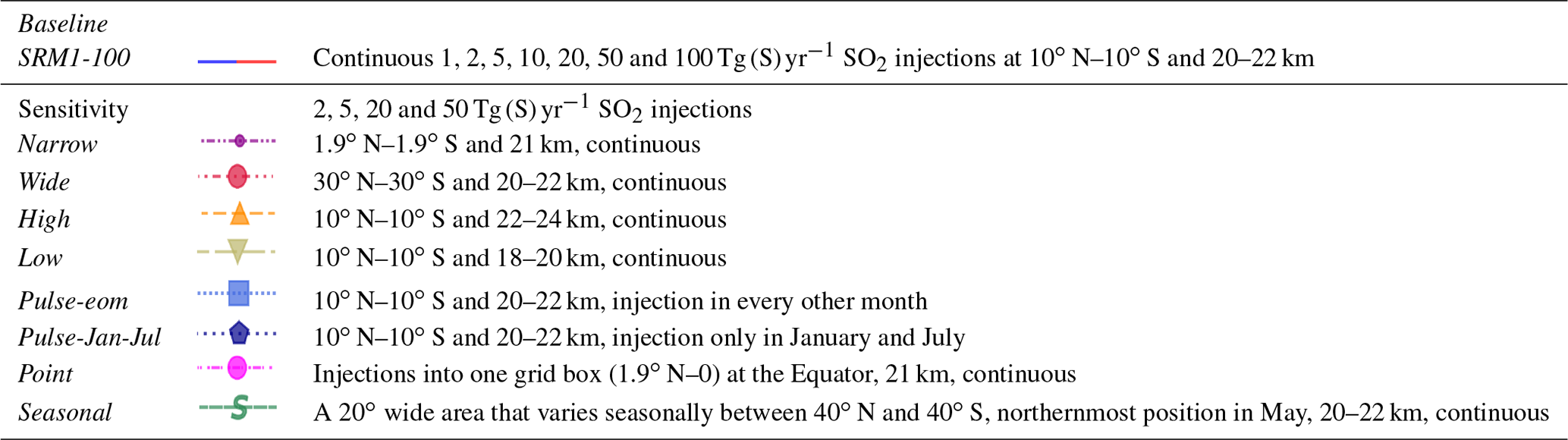
Table 1The simulated scenarios, where the line styles and markers used to indicate the scenarios in the figures are shown beside the corresponding scenario name. SALSA Baseline results are shown using blueish colours, and M7 results are shown using reddish colours in Sect. 3.1 and black in Sect. 3.3. Injections are done across all longitudes between the stated latitudes in all scenarios other than the Point scenario.
2.1.2 Modal aerosol module – M7
In M7, aerosols are represented using a superposition of seven log-normal modes: four for soluble material (nucleation, Aitken, accumulation and coarse) and three for insoluble material (Aitken, accumulation and coarse). A detailed description of M7 is found in Vignati et al. (2004), and more information on the M7 configuration of ECHAM-HAMMOZ is given in Tegen et al. (2019). The original modal set-up is designed to represent tropospheric conditions and is, therefore, not representative for cases where the lifetime of particles is long (> months), such as in case of SAI (Kokkola et al., 2009). Similarly to Niemeier and Timmreck (2015), we modify the set-up of the modes so that the coarse mode is made narrower than in the standard set-up (using standard deviation σCS = 1.2 instead of 2.0). In the case of high sulfur concentrations, a 2.0 coarse-mode width has shown to lead to a tail of large particles (Kokkola et al., 2009). Based on Kokkola et al. (2009), this caused an overestimation of the effective radius of the coarse mode, when compared with the highly resolved particle spectrum reference model, and thus increased sedimentation velocity and reduced residence time of aerosols. In M7, the median size of the mode can change, although only between mode-specific maximum and minimum threshold radii. For the nucleation mode, there is no lower threshold radius, and for the coarse mode, there is no higher threshold radius. This threshold radius also defines when aerosols are transferred from one mode to another. As in Niemeier and Timmreck (2015), we changed this threshold radius between the accumulation and coarse modes (the two largest modes) from 0.5 to 0.2 µm. Our model set-up does not include additional stratospheric chemistry, the limitation of available OH for oxidation of SO2 under extreme high-SO2 conditions (> 1000 Tg (S)) or the forced evaporation of sulfate over 30 km, as in Niemeier and Timmreck (2015) and Niemeier et al. (2021). Even though the mode set-up of the model was modified to satisfactorily represent the stratospheric aerosol at the expense of the representation of the tropospheric aerosols (especially sea salt and dust), we also include all anthropogenic emissions and natural surface emission.
2.2 Scenarios
The studied scenarios are listed in Table 1 and were simulated with both the SALSA and M7 aerosol modules. In addition, the control (CTRL) simulation without SAI was simulated with both microphysics models. In our Baseline scenario, sulfur was injected at 20–22 km altitude (three to four model vertical levels) and a band across all longitudes between the latitudes of 10∘ N and 10∘ S. To study the sensitivity of radiative forcing to the magnitude of the injection, the yearly injection rates of 1, 2, 5, 10, 20, 50 and 100 Tg(S) were used. In addition, we simulated eight sensitivity scenarios with alternative injection strategies (see Fig. S1 in the Supplement). These were done for injection rates of 2, 5, 20 and 50 Tg (S) yr−1. The Narrow and Wide scenarios were simulated to study the impacts of shrinking or widening the injection area. In the Narrow scenario, injections were done between the latitudes of 1.9∘ N and 1.9∘ S (two-grid-box-wide band) and to 21 km altitude (one model vertical level), and in the Wide scenario, sulfur was injected between the latitudes of 30∘ N and 30∘ S and the same altitude as in the Baseline scenario. The Low (injections at 18–20 km altitude) and High (injections at 22–24 km altitude) scenarios were done to study the dependency of radiative forcing on altitude. We also simulated two scenarios where injections were concentrated on certain times of the year instead of having continuous emissions over a year. In both of these scenarios the length of the one injection period was 1 month. In Pulse-eom, sulfur was injected every other month starting from January (six injection periods per year). In the Pulse-Jan-Jul scenario, sulfur was injected during 2 single months per year, January and July. In these cases, the concentration of sulfur during injections was higher compared with the Baseline scenario which had a constant injection rate throughout the year. Instead, in the Pulse-eom and Pulse-Jan-Jul scenarios, injections were interrupted outside the injection periods. This might affect the size distribution of the stratospheric aerosols.
In the Seasonal scenario, a 20∘ wide injection area is varied gradually between 40∘ N and 40∘ S throughout the year. The northernmost position (40–20∘ N) of the injection area is in May, and the southernmost position (20–40∘ S) is in November (see Fig. S1). Note that, as the injection band is always 20∘ wide (with respect to latitude) and the same mass in injected in every month, the concentration of sulfur injected is lower when the injection area is located over the Equator compared with when it is located over mid-latitudes. The results of the Seasonal and Pulse-Jan-Jul scenarios are also sensitive to the timing of injections; however, this is not studied here. The last of the studied sensitivity scenarios was Point. In Point, sulfur was only injected into one grid box located at the prime meridian instead of into a band over all longitudes.
Simulations were run over a 10-year period which included a 3-year spin-up period. Thus, a 7-year period was used in the analysis. The period length of 7 years was chosen because it covers roughly three full QBO cycles (3 × 28 months = 7 years).
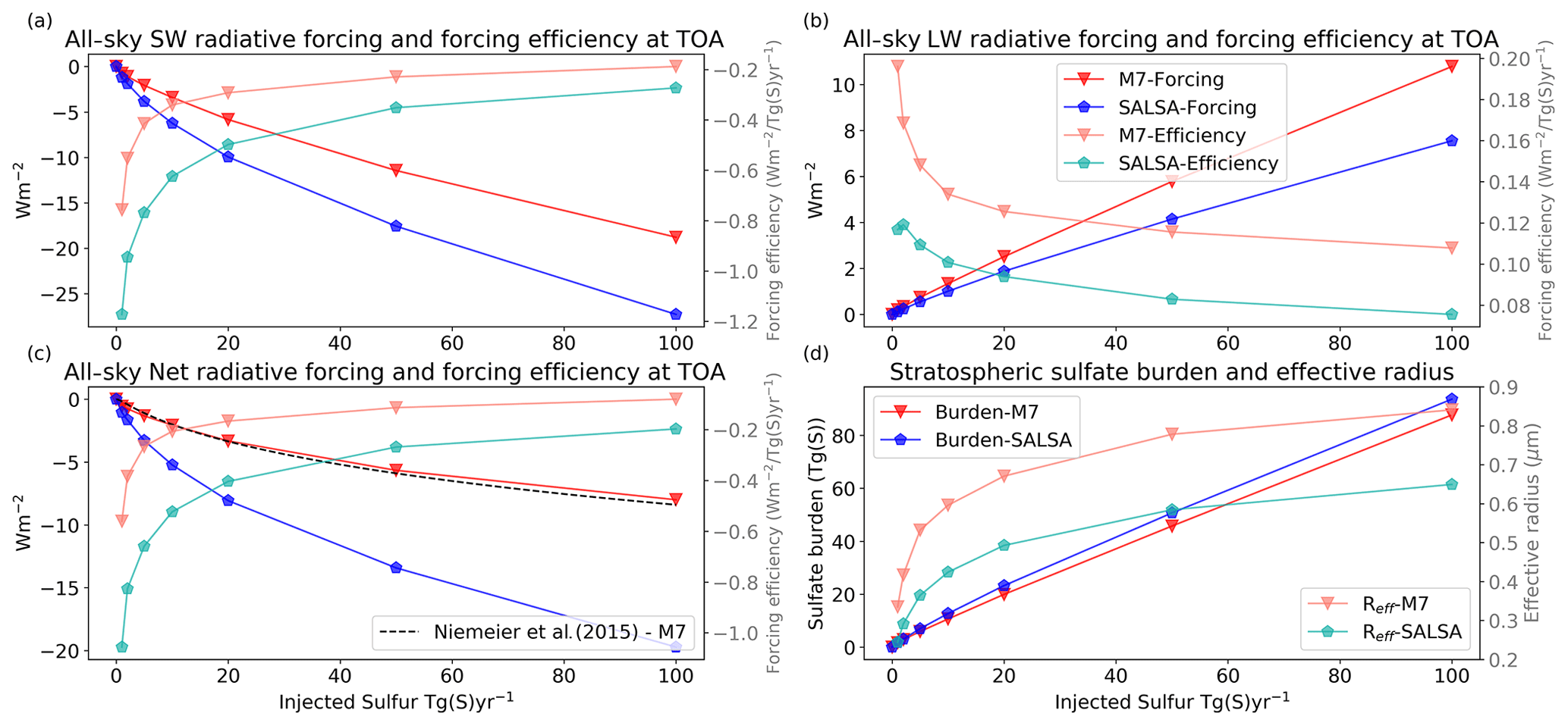
Figure 1Global mean all-sky (a) short-wave, (b) long-wave, and (c) total (net) radiative forcing and forcing efficiency as well as (d) the stratospheric sulfate burden and the mean effective radius as a function of injection rate. The M7 results are shown using red lines and markers, and the SALSA results are indicated using blue. Faint colours (forcing efficiency in panels a–c and effective radius in panel d) correspond to the right-hand faint axis.
3.1 Baseline scenarios – sensitivity to the magnitude of injections
3.1.1 The dependency of radiative forcing on the amount of sulfur injected
Figure 1 shows the dependency of the global mean all-sky SW and LW radiative forcing, the stratospheric sulfur burden, and the effective radii of aerosols on the magnitude of sulfur injection in the Baseline scenario. Results of SALSA are shown using blueish colours, and M7 results are indicated using reddish colours. The SW radiative forcing showed a sublinear increase and the forcing efficiency showed a sublinear decrease with the injection rate in both models. However, the increase in LW forcing was rather linear as a function of the magnitude of sulfur injected (Fig. 1b). This was consistent between models. Overall, because SW forcing was significantly larger than LW forcing, the net total forcing was always more negative (stronger cooling effect). However, in the case of stronger injections (> 5 Tg (S) yr−1), the LW forcing contribution to the total forcing becomes relatively higher, especially in simulations with M7. Thus, for example, the change in the total forcing in simulations with M7 was rather small (−2.09 W m−2) even though the amount of sulfur injected was doubled from 50 to 100 Tg(S) (Fig. 1c). Several studies have shown that a stronger sulfur injection will lead to relatively larger aerosols (Heckendorn et al., 2009; Pierce et al., 2010; Niemeier et al., 2011; Laakso et al., 2016). This also happens here regardless of how the aerosol microphysics is modelled. This is supported by Fig. 1d, which shows that the area-weighted mean stratospheric effective radius was increased with increasing injections.
Even though the same qualitative conclusions about the behaviour of the efficiency of SAI as a function of the amount of sulfur injected can be drawn based on both the SALSA and M7 microphysical modules, the quantitative results between the models were significantly different. The SW radiative forcing was 45 %–85 % higher in SALSA than in M7. On the other hand, the LW radiative forcing was 32 %–67 % higher in M7 than in SALSA. As SW radiative forcing and LW radiative forcing of aerosols have inverse impacts on the net radiation, this led to an even larger difference in the total net radiative forcing between models, as can be seen in Fig. 1c. With 1 and 2 Tg (S) yr−1 injection rates, the respective total radiative forcing was 88 % and 117 % higher in SALSA than in M7. In the case of higher-magnitude injections (5–100 Tg (S) yr−1), the net radiative forcing was 137 %–154 % based on simulations with SALSA compared with M7. Thus, the efficiency of stratospheric sulfur geoengineering was significantly dependent on the aerosol module used.
The net radiative forcing in our M7 simulations was in very good agreement with the results of Niemeier and Timmreck (2015), which are indicated by the black dashed line in Fig. 1c. This was at least partly a coincidence, even though M7 was used with a similar mode set-up to that in Niemeier and Timmreck (2015) here. Niemeier and Timmreck (2015) used ECHAM5-HAM instead of ECHAM6.3-HAM2.3, the latter of which was utilized in our study. Niemeier and Timmreck (2015) simulations were also done using 39 model vertical levels instead of 95, and the injection altitude was 19 km which was lower than in our simulations. In addition, the sulfur was injected into one grid box instead of along the Equator as done in our simulations. If the SALSA results presented here are compared with the results of Kleinschmitt et al. (2018), where a sectional aerosol module with 36 size bins between dry radii of 1 and 3.3 nm was used, we see a significant difference, especially in the LW radiation response. In the case of injection rates stronger than 5 Tg (S) yr−1, our simulation showed the LW forcing efficiency to be lower than 0.1 , whereas it was approximately 0.3 in Kleinschmitt et al. (2018). This means that the LW forcing was more than 2 times larger in Kleinschmitt et al. (2018) than in our simulations. The prescription of ozone was carried out in the same way in Kleinschmitt et al. (2018) and this study; thus, the different responses in LW forcing cannot be explained by the different impact of ozone on SAI. The SW forcing efficiency was slightly larger in SALSA simulations (1–2 Tg (S) yr−1), but with stronger injection rates, the results are consistent with those of Kleinschmitt et al. (2018). The dry effective radii of stratospheric aerosols with different injection magnitudes were nearly identical between the studies. This indicates that differences in radiative forcings between the studies are probably caused by differences in the LW radiation transfer (i.e due to using a different radiative transfer scheme) or differences in the aerosol optical properties in the LW radiation calculations. In addition, radiative properties of aerosols were calculated from a prescribed chemical composition consisting of 75 % H2SO4 in Kleinschmitt et al. (2018), whereas the volume-weighted average of the refractive indices of individual compounds is used in SALSA. However, it is also possible that the size distributions of aerosols were different regardless of the consistent effective radii or of how aerosols were spatially distributed in atmosphere.
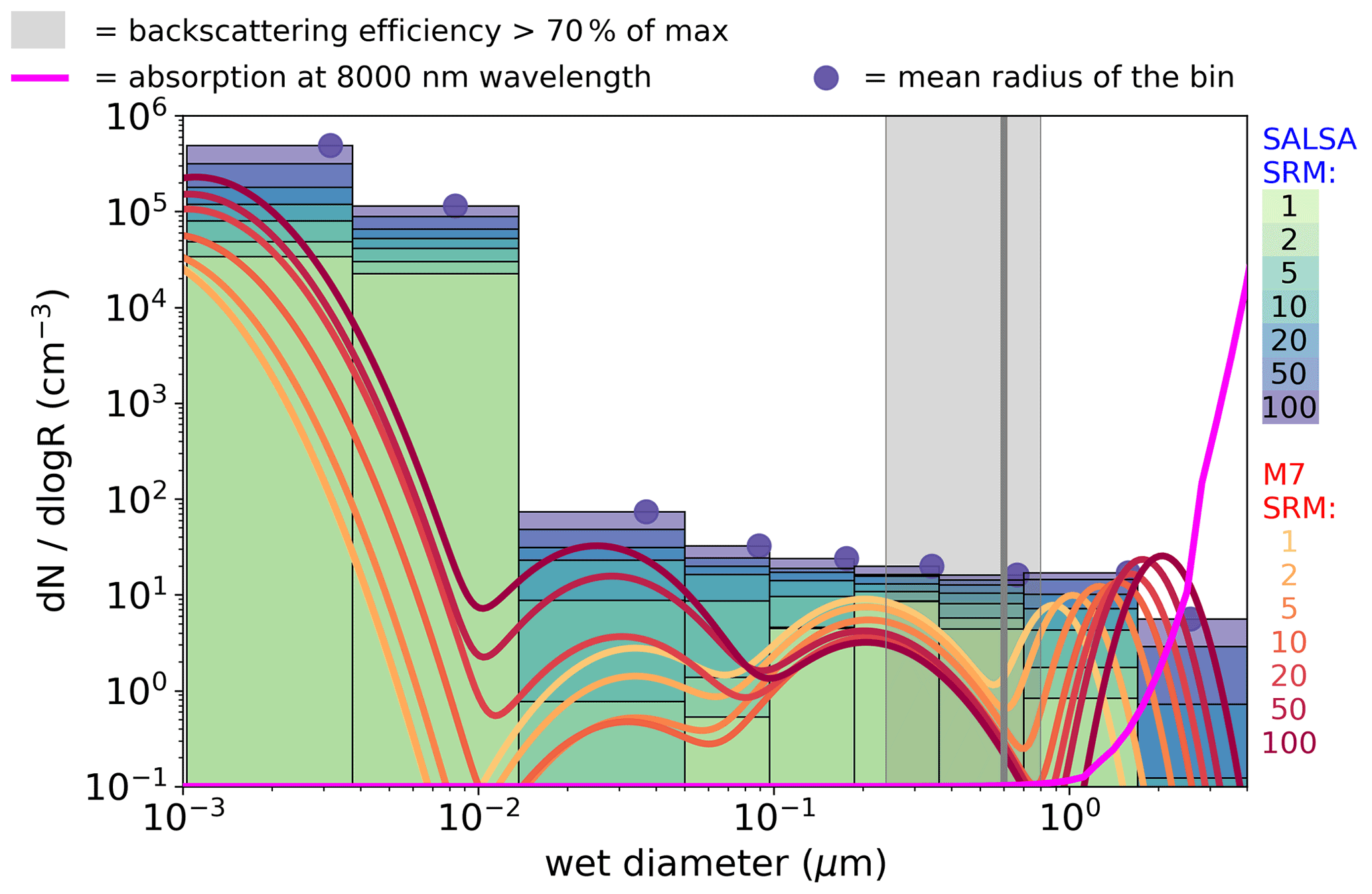
Figure 2Aerosol number size distribution at the Equator and at 20–22 km altitude in scenarios with different injection rates simulated with M7 (names of the four modes from the left: nucleation, Aitken, accumulation and coarse) and SALSA (10 size bins). For SALSA, there is not a significant number of aerosols in the largest bin; thus, it is not shown in the figure. Dots on the top of the SALSA size bins show the mean diameter of that bin for a 100 Tg (S) yr−1 injection rate. The grey line is reproduced from Fig. 5 of Vattioni et al. (2019) and shows the size for which the backscattering is maximized. The grey shaded area indicates the radius where aerosol backscattering is 70 % of the maximum from Dykema et al. (2016). The magenta line (unitless) shows the relative dependence (using a linear, not logarithmic, scale) of absorption at an 8000 nm wavelength on the (dry) diameter of the sulfate aerosols and is based on the radiation calculation module of SALSA.
Despite the fact that the radiative forcing was significantly different between the M7 and SALSA modules in this study, the stratospheric sulfur burdens were only 3 %–19 % higher in SALSA than in M7. Lower SW radiative forcing, higher LW radiative forcing and a slightly shorter lifetime is caused by less and larger sulfate particles in the M7 simulations than in SALSA. This conclusion is justified by examining the stratospheric mean effective radii (the light blue and red lines) in Fig. 1d. To analyse the aerosol size in more detail, the number size distribution along the Equator at 20–22 km altitude in the M7 and SALSA simulations for different injection rates is shown in Fig. 2. The total number concentrations were larger in SALSA than in M7 in all size classes except in particles with a diameter larger than 0.7 µm. Note that in the case of the largest injection rates, a part of the aerosols is present in the largest bin (size range of 1.7–4.12 µm), whose upper size limit goes beyond the coarse mode in M7. However, the actual mean aerosol size for that bin (purple circle in the bin) is closer to its lower limit, unlike in the other bins.
To understand the link between the size distribution and the radiative forcing, we reproduced an indicator for the size range in which the backscattering efficiency is highest, similarly to Fig. 5 of Vattioni et al. (2019). The defined size range is based on Dykema et al. (2016) and is shown as a grey shaded area in Fig. 2. The magenta line shows the dependency of the LW absorption for radiation with a wavelength of 8000 nm on the size of sulfate aerosol calculated using the SALSA radiation module for aerosols (absorption is shown here as an unitless quantity, and the scale is linear). In SALSA, the aerosol number concentration was much higher than in M7 over the size range with the highest backscattering. On the other hand, the high number concentration in the largest size range (> 0.7 µm) in M7 caused stronger LW radiative forcing than the LW forcing calculated for the SALSA-simulated size distribution. Figure 2 clearly shows why the net radiative forcing increases (becomes more negative) faster in SALSA than M7: when the injection rate was increased, the number concentration was increased in all size bins in SALSA; however, the number concentration of the accumulation-mode aerosols was decreased in M7, whereas the number concentration of the coarse mode was increased and grew in size. As seen in Fig. 2, this change is critical for LW radiative forcing because the absorption efficiency increases strongly with the aerosol size when the aerosol diameter is larger than 1 µm.
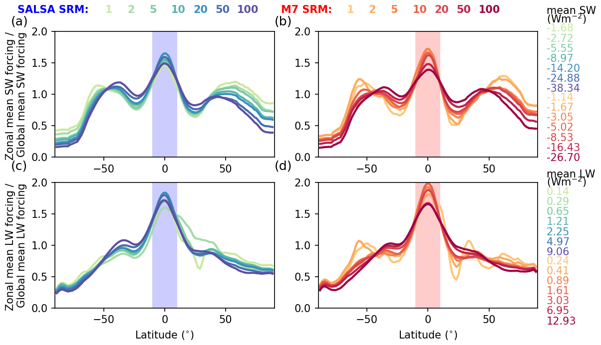
Figure 3Relative zonal distribution of (a, b) short-wave and (c, d) long-wave clear-sky radiative forcing. The zonal mean forcing in each latitude band is divided by the global mean radiative forcing of the corresponding scenario, which is shown in the legend on the right side of the figure. The blue and red shaded areas show the latitudes where sulfur was injected
Compared with the aerosol size distribution in Niemeier and Timmreck (2015), the size distribution based on the M7 simulations in our study was considerably different. The number concentrations of the Aitken and accumulation modes were much larger in Niemeier and Timmreck (2015), and the amount of accumulation aerosols increased with larger injections. These differences are probably explained by the different injection strategies. As we will show in Sect. 3.3.2, the scenario in which sulfur is injected into one model grid box, as in Niemeier and Timmreck (2015), results in a more consistent aerosol size distribution (Fig. S7b). In addition, the differences between our study and that of Niemeier and Timmreck (2015) are that a different version of the GCM and a different resolution are used in the model. Niemeier and Schmidt (2017) showed that low and high vertical resolutions led to different stratospheric dynamics which further caused differences in the aerosol sizes in SAI simulations.
3.1.2 Dependency of the zonal distribution of radiative forcing on the amount of sulfur injected
Figure 3 shows the zonal distribution of the relative clear-sky SW and LW radiative forcings (i.e. zonal/global mean radiative forcing). The maximum of the zonal mean radiative forcing was concentrated on latitude bands within the injection region over the Equator in both models (the shaded area in Fig. 3) regardless of the magnitude of injections. There were also two local maxima, especially in the zonal SW radiative forcing: 50∘ N and 50∘ S. When the injection rate was increased, the relative radiative forcing at high latitudes decreased, and the above-mentioned local maxima of the SW radiative forcing at the 50∘ latitudes moved towards low latitudes. Consequently, the relative radiative forcing increased in the tropics and subtropics while it decreased over higher latitudes. This was consistent between the models. There are two explanation for this: (1) when the amount of sulfur was increased, aerosols became relatively larger, causing a higher gravitation settling velocity, which means that fewer particles made it to high latitudes and (2) injected sulfate aerosols caused tropical stratospheric heating and a strengthening of the polar vortex, which reduced aerosol transportation to the polar stratosphere (Sect. 3.4; Visioni et al., 2020a). Thus, less sulfate aerosols were transferred to high latitudes before they were removed from the atmosphere. The variation seen in the LW radiative forcing with low injection rates (1–2 Tg (S) yr−1) is caused by background aerosols as well as the variation in the emitted LW radiation from the atmosphere and the surface due to land temperature adjustments.
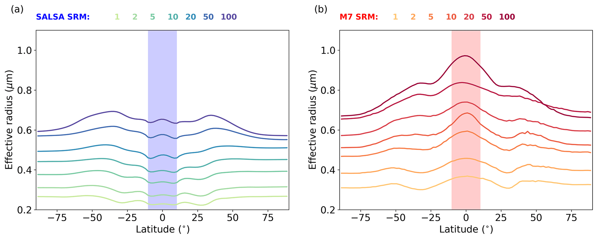
Figure 4Dependence of the zonal mean effective radius of stratospheric aerosols on the magnitude of sulfur injections simulated with (a) SALSA and (b) M7. The blue and red shaded areas show latitudes where sulfur is injected
The zonal mean effective radii were notably different between the models (Fig. 4). The impact of the injection area on the aerosol effective radii is clearly seen in SALSA between 10∘ N and 10∘ S, where the zonal mean effective radius over the injection band was smaller than over the higher latitudes. This indicates that continuous injections resulted in continuous new particle formation in SALSA. When particles were transferred out from the injection area, the effective radius began to rise due to particle growth by coagulation and condensation, while less new particles were produced by nucleation. In the M7 simulations, the effective radii were much larger over the tropics than over high latitudes. This indicates that more of the injected sulfur has condensed on pre-existing particles rather than forming new particles inside of injection area.
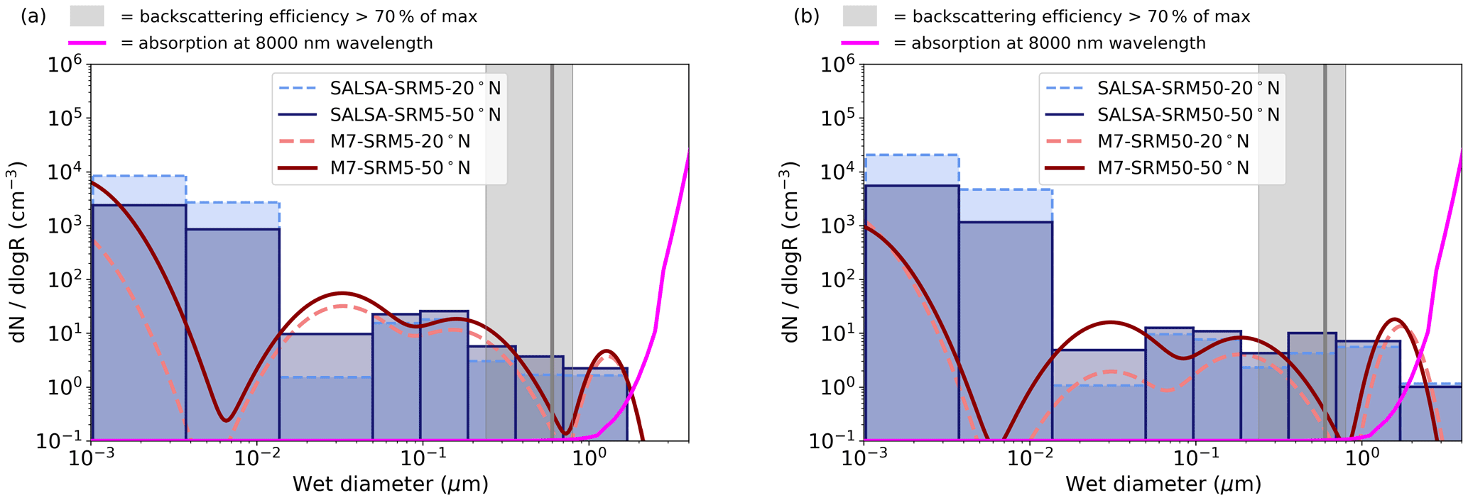
Figure 5Aerosol number size distribution at 20∘ N and 18–20 km altitude and at 50∘ N and 12–15 km altitude in the (a) SRM5 and (b) SRM50 scenarios simulated with M7 and SALSA. The grey line is reproduced from Vattioni et al. (2019) and shows the size of the maximum backscattering, and the shaded area indicates the radius where aerosol backscattering is 70 % of the maximum (from Dykema et al., 2016). The magenta line (unitless) shows the relative dependence (using a linear, not logarithmic, scale) of absorption at an 8000 nm wavelength on the (dry) diameter of the sulfate aerosols, based on the radiation module of SALSA.
Figure 5 shows the aerosol number size distribution over 20 and 50∘ N. When the aerosol plume moved towards high latitudes, the number of the Aitken- and accumulation-mode aerosols began to increase and coarse-mode aerosols began to decrease compared with the size distribution over the Equator. Thus, the aerosol effective radii over 20 and 50∘ N were much smaller compared with the effective radius at the Equator. In SALSA, the number size distribution at 20 and 50∘ N was trimodal in shape, whereas at the Equator, excluding two smallest bins, it was relatively monodisperse. At 50∘ N, the number size distribution and effective radius were more consistent between models than closer to the injection area. However, there is still a gap between the accumulation and coarse modes in M7.
In addition to radiative impacts, the size of the aerosols affects where and how fast particles are removed from the atmosphere. As Fig. S2 shows, deposition was much faster in the tropics (32 % for a 50 Tg (S) yr−1 injection rate) in M7 than in SALSA, whereas the deposition of sulfur outside the tropics was lower (roughly 10 % in SRM50). This conclusions holds regardless of the amount of sulfur injected. Figure S3 shows that, in the case of a 50 Tg (S) yr−1 injection rate, the deposition of sulfate is clearly faster in SALSA than in M7 (e.g. over Europe and the USA). Enhanced sulfate deposition due to SAI might offset or even exceed the impacts of a reduction in anthropogenic SO2 emissions which might have negative impact on ecosystems in these regions (Visioni et al., 2020b).
3.2 Analysing the causes of differences between the SALSA and M7 results
Based on Fig. 4, there was a significant difference in the evolution of aerosols within the injection band between the two models. In this region, large amounts of gaseous H2SO4 is constantly produced from continuous SO2 injection and oxidation by OH. In the stratosphere, the conditions are favourable for new particle formation through H2O–H2SO4 binary nucleation, but there is also a large amount of pre-existing sulfate aerosols to which gaseous H2SO4 can condensate. These two processes compete for available gaseous H2SO4, and solving them simultaneously in the model is challenging especially when sulfur concentration is high; this can lead to large biases (Kokkola et al., 2009; Wan et al., 2013). SALSA and M7 allocate the amount of sulfuric acid partitioning from gas to particles between new particle formation and condensation differently. Based on the results, most of the gaseous sulfate is partitioned into new particle formation in SALSA, whereas little goes into condensation. In addition, there is a condensation sink in SALSA due to the high number of particles smaller than 10 nm that does not exist in M7; thus, there is less gaseous sulfuric acid to condense to the larger particles. On the other hand, the number concentration of particles smaller than 10 nm at the Equator in M7 was only 34 % of the number concentration in SALSA, and, as Fig. 4 shows, the effective radius in M7 was larger inside the injection region compared with latitudes at which injections did not take place. This indicates that new particle formation is much lower in M7 than in SALSA and that sulfate gas condensates onto existing particles inside the injection area, which results in a larger number and size of coarse-mode particles compared with latitudes at which no injection takes place.
In M7, the coupling of nucleation and condensation is done using a two-step time integration scheme proposed by Kokkola et al. (2009). Based on Wan et al. (2013), this has been shown to cause a negative bias for the nucleation sink and a positive bias for the condensation rate. In SALSA, the operator-splitting technique (Jacobson, 2002) is used (Bergman et al., 2012). In this method, the nucleation rate is added to the condensation mass transfer rate in the first size bin. Based on the test simulations with the box model (not shown), when nucleation takes place, it outcompetes condensation, and there is significantly less condensation. This conclusion is supported by Fig. 4a, which shows that the effective radius is clearly smaller at latitudes in which injections take place compared with higher latitudes. It is not clear if this is caused by an overestimation of the nucleation rate, an underestimation of the condensation rate, or the method used for solving nucleation and condensation simultaneously. However, to study the size of the impact of competition between nucleation and condensation on the different results between models, we carried out additional simulations where competition was excluded in both models. These results are shown in the Appendix. In these simulations, nucleation was switched off, and 25 % of the injected sulfur mass was assumed to be primary particles that were 3 nm in diameter while the rest was injected as SO2. With the original set-up, 5 Tg (S) yr−1 or higher injection rates simulated with SALSA showed a 137 %–147 % larger global mean all-sky net radiative forcing than in M7. When nucleation was replaced by injecting 25 % of the sulfur as 3 nm particles, the radiative forcing was now only 78 %–99 % larger in SALSA than in M7. Thus, these simulations showed that excluding nucleation brought the global mean net radiative forcing results between the models closer to each other, although a significant difference remained. This is because there is not a large difference in the aerosol number size distribution for particles larger than 0.1 µm between the Baseline simulations and the modified simulations without nucleation (see Fig. A3 in the Appendix). Thus, most of the differences in the radiative forcing between models are not caused by differences in the calculated competition between nucleation and condensation.
In M7, the aerosol size classes are more restricted to the definition of the modes than in SALSA which uses bins. In M7, the mode widths are fixed. The mean radius of the each mode can change, but it has fixed low and high limits; for example, in the set-up used in this study, the accumulation mode (second-largest mode) has low and high radius limits of 0.05 and 0.2 µm respectively. These limits define the average mass of the mode. If the average mass of the particles in the mode exceeds the average mass defined from the lower and upper limits, the transfer of number and mass to the next mode occurs. The impact of this can be seen in Fig. 2. In all M7 simulations, regardless of injection rate, the average mass of the accumulation mode was close to the upper limit. Thus, it cannot grow by condensation or coagulation because gained extra mass is always transferred to the coarse mode. This also decreases the number of accumulation-mode particles. The number concentration of the accumulation mode can only increase by the coagulation of two smaller particles or through the growth of the Aitken mode. However because coagulation between larger and smaller aerosols is more efficient than between two small aerosols, and because the number of coarse-mode particles is high, the Aitken mode cannot compete with the coarse mode as a coagulation sink for nucleation- and Aitken-mode aerosols. Hence, fewer Aitken-mode aerosols can grow to the accumulation-mode size by coagulation. This creates a self-reinforcing loop in which the number and mass of the coarse mode increase.
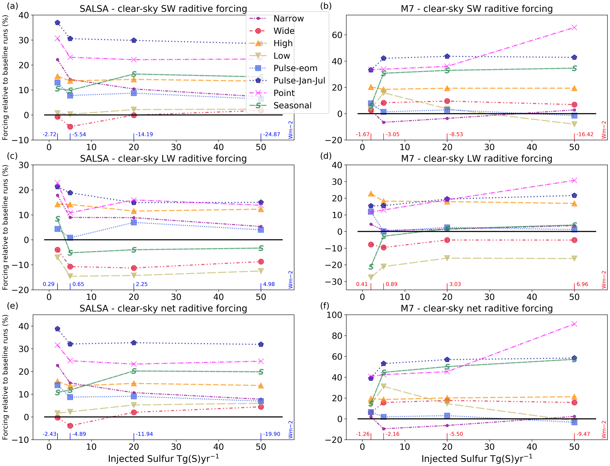
Figure 6Relative global mean clear-sky SW (a, b), LW (c, d) and net radiative forcing in sensitivity scenarios compared with the Baseline scenario and its corresponding sulfur injection rate. Baseline values are shown at the bottom of each panel. SALSA results are shown in panels (a), (c) and (e), and M7 results are shown in panels (b), (d) and (f). Note the different y-axes scales between the panels.
Because the size range of the accumulation mode is restricted by the upper limit, whereas coarse-mode aerosols become larger with increasing injection size, there is a gap in the size distribution between these two modes where the aerosol number concentration is low (Fig. 2). Coincidentally, this gap is located at the size range of the largest backscattering efficiency, which is indicated by the grey shaded area in Fig. 2. Thus, the modal set-up of M7 causes a numerical limitation on the particle size distribution which, in this case, has an impact on the efficiency of SAI. Note that, based on the earlier SAI simulations using M7 in Niemeier and Timmreck (2015), the threshold radius at which aerosols from the accumulation mode are transferred to the coarse mode was set to 0.2 µm (0.5 µm in standard set-up).
The above-mentioned differences in the responses between models can easily go unnoticed when models are evaluated against measurements after a large volcanic eruption. Because Mt. Pinatubo is the only large volcanic eruption that has taken place during a period for which proper observations of stratospheric aerosols' radiative properties are available, it has often been used as a test case with respect to models' capability to simulate stratospheric aerosols (e.g. English et al., 2013; Mills et al., 2017; Niemeier et al., 2009; Laakso et al., 2016; Sukhodolov et al., 2018). However, based on our results, it probably does not give a reliable picture of models' capability to simulate stratospheric sulfur injections for SAI. For example, both of the models used here have been shown to represent the effective radius of sulfate aerosols and the burden of sulfur after the Mt. Pinatubo eruption relatively well (Niemeier et al., 2009; Laakso et al., 2016); in particular the models' results were shown to be in very good agreement with each other (see Fig. 16 in Kokkola et al., 2018). However, the models' responses are significantly different with respect to SAI. This is because the background conditions in the case of a volcanic eruption and continuous sulfur injections are significantly different: during a volcanic eruption, sulfur is erupted into a relatively particle-free stratosphere, whereas during SAI, sulfur is injected into an existing particle field in the stratosphere. In the former case, competition between nucleation and condensation does not play as large of a role as it does in SAI. The gap in the size distribution is also widened as a consequence of continuous injections in a band across all longitudes because the accumulation mode cannot grow whereas the coarse mode becomes larger (due to continuous injections). The gap is narrower for point-like injections, as we see in the next section. This also indicates that a clear gap, such as that in our Baseline scenario, does not occur in a simulation of a large volcanic eruption.
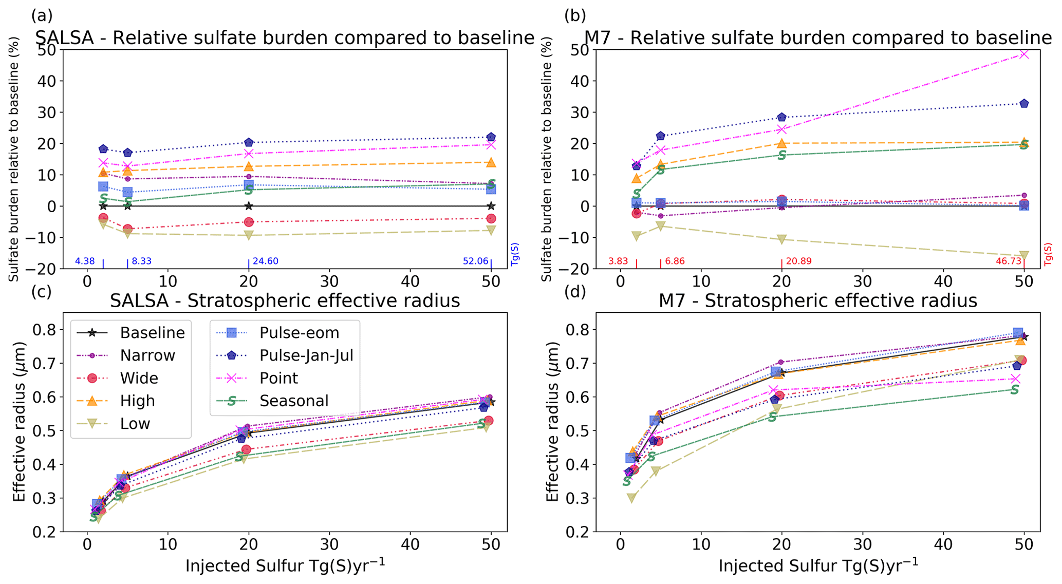
Figure 7(a, b) The relative stratospheric sulfur burden in sensitivity scenarios compared with the Baseline scenario with its corresponding sulfur injection rate. (c, d) The global mean effective radius of stratospheric aerosols

Figure 8Zonal mean clear-sky net forcing with (a, b) 5 and (c, d) 50 Tg (S) yr−1 injection rates in simulated sensitivity scenarios. SALSA results are shown in panels (a) and (c), and M7 results are shown in panels (b) and (d). Note that the y axes show negative (cooling) values. Shaded areas show the latitudes of the injection area at the time of year (month shown on the right y axes of panel a) for each injection scenario. Latitudes of the injection area are the same in the Baseline, High and Low scenarios (10∘ N–10∘ S).

Figure 9Zonal mean effective radius of stratospheric aerosols in the studied sensitivity scenarios for (a, b) 5 and (c, d) 50 Tg (S) yr−1 injection rates simulated with (a, c) SALSA and (b, d) M7.
3.3 Sensitivity scenarios – sensitivity to injection strategy
In this section, we investigate the impact of various injection strategies on the geoengineering efficiency and the zonal distribution of the radiative forcing as well as how the responses depend on the model used. The descriptions of the sensitivity scenarios are found in Table 1. Figure 6 shows the relative difference in the global mean clear-sky SW, LW and net radiative forcing compared with the Baseline scenario for a corresponding injection magnitude. The relative sulfate burdens compared with the Baseline scenario and the effective radii of stratospheric aerosols are shown in Fig. 7, and the tabulated values are given in the Supplement (Tables S1 and S2). The zonal mean net clear-sky radiative forcing is shown in Fig. 8. The zonal mean effective radius of stratospheric aerosols is shown in Fig. 9. We show the clear-sky radiative forcing here instead of the all-sky forcing, as it is more straightforward to compare the radiative forcings to the aerosols size under clear-sky conditions because clouds do not affect the results. Figures for all-sky radiative forcings and the tabulated absolute values of clear-sky and all-sky SW, LW and net radiative forcings are shown in the Supplement (Figs. S4 and S5 and Tables S1 and S2).
3.3.1 Sensitivity to the width of the injection area
To investigate the sensitivity of the radiative impacts of SAI to the width of the injection area, we studied the injection of sulfur to bands with widths of 4∘ (Narrow), 20∘ (Baseline) and 60∘ (Wide) over the Equator. The responses of the radiative forcing to the widening of the injection area from 20 to 60∘ were similar in both models. The effective radii of stratospheric aerosols were smaller and the LW radiative forcing was lower in both models compared with the Baseline scenario. Widening the injection area affects the radiative forcing in two ways. First, it decreases the mean sulfate concentration over the tropics and results in relatively more and smaller particles. These effects are shown as smaller effective radii (Fig. 7) and lower absorption of LW radiation by the smaller particles. Second, injecting sulfur farther from the Equator, where the solar intensity is largest on average, decreases the potential of aerosols to scatter radiation. Thus, widening the injection area also decreases the lifetime of aerosols because some of the aerosols are injected closer to high latitudes, where they are removed faster than over the low latitudes. In SALSA, where the condensation on the existing particles is weaker than in M7, concentrating the sulfur injection over a wider area does not matter as much as in M7 in a microphysical sense, as nucleation occurs at the expense of condensation even at high sulfur concentrations. Thus, the lifetime of aerosols in SALSA is reduced due to their more efficient removal when injected into higher latitudes compared with the Baseline scenario. In M7, there is not large difference in the lifetime of aerosols between the Baseline and Wide scenarios. Overall, the global mean total (SW and LW) radiative forcing was roughly 20 % larger than in the Baseline scenario when simulated with M7, whereas the difference was between ± 4 % with SALSA depending on the injection rate.
A wider injection area decreases the radiative forcing over the tropics while increasing it at higher latitudes compared with the Baseline scenario (Fig. 8). However, the difference in radiative forcings at the tropics with a 50 Tg (S) yr−1 injection rate between the Baseline and Wide scenarios was rather small in M7 (< 10 %). In the Baseline scenario, a higher injection concentration due to the narrower injection area (10∘ N–10∘ S) causes the effective radius of stratospheric particles in M7 to be larger than 0.8 µm, which is not an optimal size for scattering radiation (Fig. 9).
As expected, a narrower injection area (two model grid boxes over the Equator; Narrow scenario) led to larger effective radii of stratospheric aerosols in both models compared with the Baseline scenario. However, the sulfur lifetime increases as sulfur is injected into stratospheric tropical pipe. As for the Wide scenario, the impact of the locally larger injection rate does not increase the effective radii of aerosols in SALSA as much as it does in M7, and the lifetime of particles was 10 % longer in the Narrow scenario compared with the Baseline scenario due to the impact of atmospheric circulation. Thus, the radiative forcing of the Narrow injection scenario was larger than in the Baseline scenario, and it decreased gradually from 23 % to 8 % when the magnitude of sulfur injections was increased from 2 to 50 Tg (S) yr−1, based on SALSA simulations. Simulations with M7 show that the Narrow injection strategy does not significantly affect the lifetime of aerosols, and the net radiative forcing in the Narrow scenario was of the same magnitude or slightly lower than in the Baseline scenario in M7.
3.3.2 Injecting into one grid box instead of into a band over longitudes
In the Point scenario, the injection area in Narrow was also decreased in the meridional direction, reducing it to one grid box. This further increased the sulfur injection rate in the injection area, as sulfur injections are concentrated in a smaller region. However, as injection takes place longitudinally in an area that is one grid box wide, existing aerosols over the Equator from previous injections are generally not condensation or coagulation sinks for injected sulfur in the injection area, as is the case when injections occur across all longitudes. Even though sulfur mixes relatively fast over longitudes, the available gaseous sulfate for condensation or nucleation is localized near the injection area in the Point scenario.
Based on simulations with SALSA, the Point scenario was the second-most efficient SAI strategy in this study, regardless of the magnitude of injections. The mean net clear-sky radiative forcing in the Point scenario was 23 %–32 % larger than in the Baseline scenario, depending on the injection rate. The results of the Point scenario with M7 showed significantly different behaviour when increasing the injection rate compared with the other scenarios and even when compared with the same scenario when SALSA was used instead of M7: while the clear-sky global mean net radiative forcing was roughly 40 % larger compared with the Baseline scenario with an injection rate of 2, 5 or 20 Tg (S) yr−1, it was 91 % larger in the case of an injection rate of 50 Tg (S) yr−1. To study this in more detail, additional simulations of the Point injection scenario were run with M7 and with 10, 30, 40, 70 and 100 Tg (S) yr−1 injection rates. The global mean SW radiative forcing, the forcing efficiency, and the lifetime and effective radius of stratospheric aerosols from these simulations are shown in Fig. S6. All simulations with SALSA and all other scenarios with M7 showed the following: the effective radius increased and the SW radiative forcing efficiency and lifetime of aerosols decreased with an increasing injection rate. However in the Point scenario with M7, the lifetime of aerosols increased with increasing injection rate when injection rates were larger than 20 Tg (S) yr−1. In addition, the SW forcing efficiency did not decrease and the effective radius of stratospheric aerosols did not increase gradually with the injection rate as in simulations with SALSA and in all of the other scenarios.
A closer look at the aerosol number size distributions over the Equator in the Baseline and Point scenarios shows why the lifetime and SW radiative forcing increased in the Point scenario with an increasing injection rate (Fig. S6). In the Baseline scenario, the number concentration of accumulation-sized aerosols decreased whereas the number and size range of the coarse mode increased with increasing injection rate. This did not happen in the Point scenario, where the number of accumulation-mode aerosols increased and the median radius of the coarse mode did not grow the same way as in the Baseline scenario. In addition, when the injection rate exceeded 30 Tg (S)−1, the coarse mode shrank with increasing injection rates, which probably explains the increase in the mean lifetime of aerosols. This also contradicts the results of Niemeier and Timmreck (2015), who found that the size of the coarse mode increased with the injection rate in a simulation of injections into one grid box.
It is not totally clear what is causing this peculiar behaviour in this one specific scenario in M7. The scenario, where sulfur is injected into a single grid box, differs from all others in two ways. First, the concentration of injected SO2 is significantly higher compared with scenarios with injections over a whole latitude band; as was pointed out earlier, this may lead to an OH limitation for sulfate formation, which is not simulated with prescribed chemistry. Second, in the Point scenario, aerosols over the Equator do not experience continuous injections except in one model grid box. Inside the injection area, the concentration of nucleation particles is high, and these particles can grow to the size range of the Aitken mode due to self-coagulation and condensation. This is seen as a larger number concentration at the longitude where injections take place (Fig. S8b). If compared, for example, to the size distribution of the Baseline scenario (Fig. 2), the number concentration of Aitken-mode aerosols is significantly higher; thus, this mode can also compete more efficiently with the coarse mode for available sulfate gas. This results in a larger number of accumulation-mode aerosols than in the Baseline scenario and, thus, a larger SW radiative forcing. On the other hand, the size of the coarse-mode particles is significantly smaller in the Point scenario than in the Baseline scenario. The mean radius of the coarse mode is affected by several processes: coagulation and condensation on the coarse-mode aerosols increase the size of the coarse mode, whereas the sedimentation and reallocation of aerosols from the accumulation mode to the coarse mode decrease the mean radius. It seems that, with a high enough injection rate (more than 30 Tg (S) yr−1), the processes contributing to the shrinking of the mode are more efficient, resulting in an overall decrease in the size of the coarse mode. In addition, coarse-mode particles that are carried around the Equator experience continuous injections in the Baseline scenario and grow to a larger size due to the efficient condensation; they also coagulate efficiently with the new particles that are formed. In the Point scenario, this does not happen, as there is significantly less available H2SO4 outside of the injection area (Fig. S8a).
As previously mentioned, this peculiar behaviour was not seen in Niemeier and Timmreck (2015), who simulated a similar scenario with the M7 module in an earlier generation of ECHAM. However, as the atmospheric model, the background conditions (e.g surface aerosol emissions) and the resolution were different from those in this study, this peculiar behaviour might be somehow related to atmospheric dynamics (Niemeier and Schmidt, 2017). This indicates that the unique behaviour seen in the lifetime of aerosols and radiative forcing in the Point scenario is probably caused by non-linearities in the microphysical processes and dynamical changes and restriction of modes in the aerosol size distribution in M7. This shows that simulating extreme cases, where the sulfur concentration is locally large, might lead to peculiar behaviour in a modal model. This should be kept in mind when simulating events such as supervolcanoes. In any case, the significant difference in model responses seen between M7 and SALSA with respect to SAI and these peculiar results in the Point scenario highlight the need for better tools or observational data to evaluate models.
Zonally, the Point scenario led to the largest radiative forcing at the Equator out of all studied scenarios in both models. Most notably, Point stands out in the simulations of a 50 Tg (S) yr−1 injection rate with M7, where the radiative forcing is 230 % larger over tropics compared with the Baseline scenario. In addition, radiative forcing over the tropics in the Point scenario with M7 was close to the results of the Baseline scenario with SALSA even though simulations with SALSA generally showed much larger radiative forcing. Several studies have shown that offsetting the average GHG-induced global warming using SRM leads to cooling at the tropics and warming at high latitudes in the case of equatorial injection or, in an idealized case, where SRM is imitated by reducing the solar constant (Aswathy et al., 2015; Jones et al., 2016; Kravitz et al., 2016; McCusker et al., 2012; Yu et al., 2015). Even though injecting sulfur to one grid box turned out to be an efficient injection strategy in the simulations of both models, the cooling is strongly concentrated over the tropics. The Point injection strategy might make the fundamental problem of SRM, where the tropical region is cooled more at the expense of warming the high latitudes, worse if injections are concentrated in the tropics.
3.3.3 Sensitivity to injection altitude
Several studies have shown that the lifetime and the radiative forcing of stratospheric aerosols increase with the altitude of injections due to a longer sedimentation path (Heckendorn et al., 2009; Niemeier et al., 2011; Kleinschmitt et al., 2018; Vattioni et al., 2019; Tilmes et al., 2018b). Here, we studied the impact of injection altitude using three scenarios – Low, Baseline and High – where sulfur is injected at altitudes of 18–20, 20–22 and 22–24 km respectively. When comparing the High scenario to the Baseline scenario, our results with both models were consistent with previous studies. The injection rate did not have a large impact on how the radiative forcing of sulfur injection at high altitudes compares with the results of our Baseline scenario. Injecting sulfur into a higher altitude led to a 14 %–16 % larger net radiative forcing compared with the Baseline scenario when simulated with SALSA. With M7, the High scenario led to a 7 %–15 % larger net radiative forcing than the Baseline scenario. As Fig. 7 shows, injection at higher altitude led to effective radii values close to results of the Baseline injections, while the stratospheric sulfate burden was 12 %–20 % larger in simulations with both models. This indicates that the larger radiative forcing in the High injection scenario is caused mainly by a longer sedimentation path, and the size distribution of aerosols is not significantly affected by the differences in the microphysical processes due to the injection altitude.
Our results indicate that the impact of atmosphere dynamics on aerosol microphysics had a clearly larger role when injecting at a lower altitude (18–20 instead of 20–22 km in Baseline). While the lifetime of aerosols was reduced as expected (Fig. 7a,b) because of the shorter sedimentation path, the effective radii were also clearly smaller than in the Baseline scenario. This is consistent between the microphysical models. Simulations with SALSA showed that injecting sulfur at lower altitude enhanced net clear-sky radiative forcing by 2 %–6 % compared with radiative forcing in the Baseline scenario. In M7, the radiative forcing was 14 %–21 % larger than in the Baseline scenario in the case of an injection rate of 2–20 Tg (S) yr−1, but a 50 Tg (S) yr−1 injection rate led to roughly the same global mean radiative forcing as in the Baseline scenario.
Smaller aerosols in the Low scenario compared with Baseline originated from differences in the atmospheric circulation at different altitudes. Figure S9 shows the average meridional wind speed in the Low scenario with 5 Tg (S) yr−1 injection rates simulated with M7. In Low, when injecting into lower altitude (18–20 km), the mean wind patterns point from the Equator to higher latitudes. Winds carry more aerosols from the Equator to high latitudes, which reduces the sulfur concentration over the Equator compared with the Baseline scenario. This conclusion can also be drawn by analysing where SO2 is oxidized to sulfate. A 5 Tg (S) yr−1 injection rate with M7 shows that 10 %–30 % less sulfate is produced via SO2 + OH over the Equator in the Low scenario than in the Baseline, whereas sulfate production is 10 %–50 % higher in the subtropics and mid-latitudes (Fig. S9). As there is less H2SO4 gas over the Equator to condensate on the existing particles, particles are smaller in the Low scenario than in the Baseline scenario. Moreover, due to the atmospheric circulation, which more efficiently transports aerosols to higher latitudes, the zonal radiative forcing is concentrated more on mid-latitudes than the tropics for injections into lower altitudes compared with the Baseline scenario (Fig. 8).
Our conclusions on the sensitivity of the radiative forcing to the injection altitude differ from the conclusions of Niemeier and Schmidt (2017). Their study showed that injecting sulfur at an altitude of 60 hPa (19 km) resulted in a larger radiative forcing than injecting sulfur at 30 hPa (25 km) when the injection rates were larger than 10 Tg (S)−1. Here, in our simulations, the Low scenario led to a larger radiative forcing compared with injections into the altitude (20–22 km) used in the Baseline scenario, even for an injection rate lower than 10 Tg (S)−1. In addition, in the case of a 50 Tg (S)−1 injection rate simulated with M7, the model results did not show a large difference in the global mean radiative forcing between the Low and Baseline scenarios. When comparing to our High (22–24 km) scenario, which is close to the higher altitude studied in Niemeier and Schmidt (2017), the radiative forcing from the Low injection strategy was higher only in the case of a 5 Tg (S) yr−1 injection rate simulated with M7. However, in Niemeier and Schmidt (2017), sulfur was injected into one grid box, whereas in this study, sulfur was injected into a band across all longitudes and a different model version and resolution were used. Overall, this means that a universal conclusion regarding how the injection altitude affects direct aerosol radiative forcing cannot be drawn, as the results depend on the atmospheric circulation in the altitude where injections take place as well as on the injection rate and width of the injection area.
3.3.4 Sensitivity to the temporal variation of injections
In addition to scenarios where sulfur was injected continuously over a year, we studied two scenarios where the injections were concentrated only on a certain time of year: in the Pulse-eom scenario, injections were done during every second month starting from January; in the Pulse-Jan-Jul scenario, injections were done in 1-month-long periods twice per year, in January and July. Results from the Pulse-eom scenario were close to results of the Baseline injection strategy in both models. The 1-month frequency between suspending the injection and restarting it is relatively short compared with the time required for transportation, oxidation or growth of the particles to have a significant impact on results compared with continuous injections over the year. Some of the aerosols moved out from the injection area during the pause in injections, which decreased condensation and coagulation on the existing particles over the Equator compared with the Baseline scenario. However, in the Pulse-eom scenario, the injection rate at the time of the injection is doubled. In SALSA, the latter does not decrease radiative forcing efficiency as much as in M7 due to more efficient nucleation at the expense of condensation. Thus, in SALSA simulations, the lifetime of aerosols was roughly 5 % longer and the global mean radiative forcing was 10 %–15 % larger in Pulse-eom than in the Baseline scenario. Simulation with M7 did not show a significant difference in the global mean radiative forcing between the Baseline and Pulse-eom scenarios (−3 %–7 %).
In the Pulse-Jan-Jul scenario, the amount of injected SO2 was 6 times larger during the injections compared with continuous injections. However, there was a 5-month period where the injections were suspended and aerosols had time to transfer to higher latitudes before the next injection period was started. Thus, when a new injection period started, there were less particles from the preceding injections present over the Equator. Hence, condensation on existing particles and coagulation between the new and old particles were lower than in the case of continuous injections. This reduces the particles' average size compared with Baseline injections. The zonal effective radius was smaller at all latitudes compared with the Baseline scenario in both models and for all injection magnitudes (see Fig. 9). This enhanced the lifetime of aerosols by 17 %–35 % with M7 and by 20 %–27 % with SALSA. Based on SALSA simulations, the forcing efficiency of the Pulse-Jan-Jul scenario was the largest of all of the studied scenarios, as the forcing was over 30 % larger than in the Baseline scenario. The results of M7 even show a larger radiative forcing for the Pulse-Jan-Jul scenario compared with Baseline, and its relative radiative forcing increased gradually from 40 % to 58 % when the injection rate was increased from 2 to 50 Tg (S) yr−1.
It is expected that the results of the scenario in which sulfur is injected only during certain months are sensitive to the months that injections take place in and to the length of the injection periods. Atmospheric circulation varies during the year, and the transport and growth of aerosols are dependent on the timing of the injections. In addition, the seasonal cycle of solar radiation and how it coincides with the aerosol field has a large impact on the efficiency of SAI as well as on the available OH for the oxidation of SO2. As shown by Visioni et al. (2019), radiative forcing is significantly dependent on the season in which injections takes place.
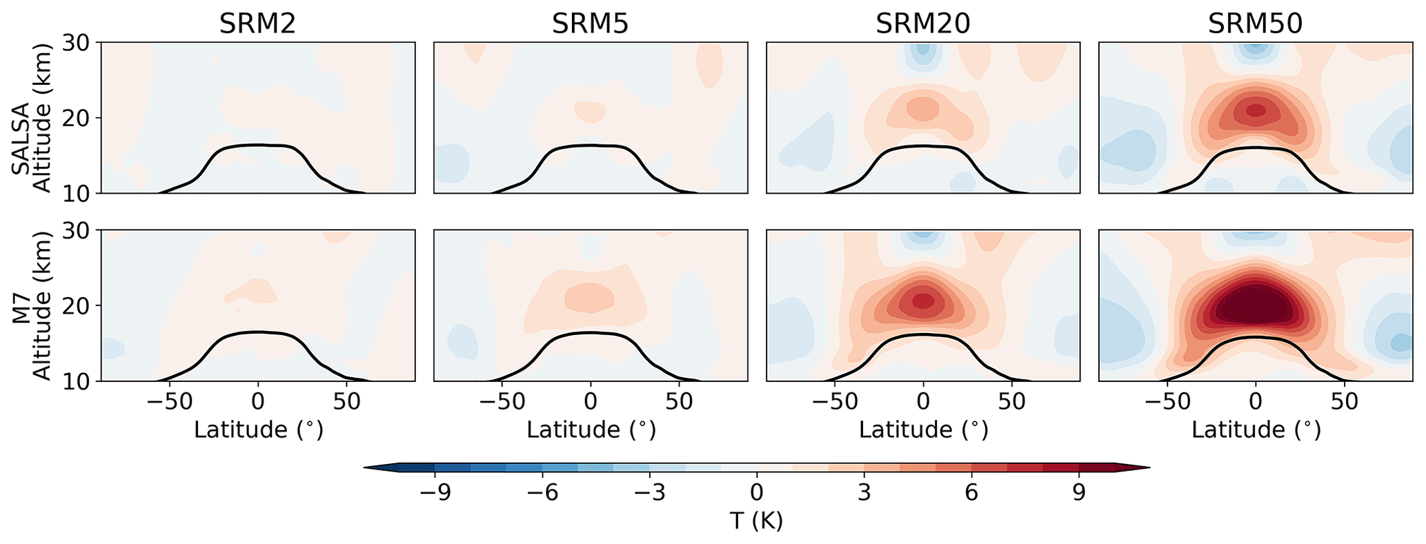
Figure 10The temperature anomaly due to the Baseline stratospheric sulfur injection with different injection rates simulated with SALSA (upper panels) and M7 (lower panels). The black line indicates the tropopause.
3.3.5 Seasonally changing injection area
The last of the studied scenarios was one where a 20∘ wide injection area was varied gradually between 40∘ N and 40∘ S during the year (the Seasonal scenario). As suggested in Laakso et al. (2017), the aim of a seasonally changing strategy is to increase the efficiency of SAI compared with continuous equatorial injections by targeting the aerosol fields to coincide with maximum solar radiation during the year and reducing the particle size by varying the injection area so that sulfur is not always injected into regions where there are pre-existing larger aerosols from preceding injections. Another objective is to produce relatively less cooling in the tropics and more cooling at middle and high latitudes compared with continuous equatorial injections. This could prevent the overcooling of the tropics and undercooling of the polar regions in cases where the average GHG-induced warming is offset by equatorial injections (Laakso et al., 2017).
Figure 6 shows that, based on SALSA simulations, the global mean clear-sky radiative forcing of the Seasonal scenario was 10 %–20 % larger compared with Baseline scenario. Simulations with M7 also showed a significant enhancement in the global mean radiative forcing, especially with injection rates higher than 5 Tg (S) yr−1 for which the radiative forcing was 45 %–57 % larger than in the Baseline scenario. The size of the stratospheric aerosol was also smaller, and Fig. 7 shows that the effective radius of stratospheric aerosols in the case of seasonal injections was clearly smaller compared with equatorial injections. Further, Fig. 8 shows that the clear-sky zonal mean radiative forcing was concentrated in the mid-latitudes rather than over the tropics.
Here, the variation of the injection area between latitudes in the Seasonal scenario was implemented so that the northernmost position (40–20∘ N) takes place in May. The results of the seasonal injection strategy are sensitive to the phase when the northernmost/southernmost position occurs. This affects the probability of optimally sized particles coinciding with maximum incoming solar radiation, how fast SO2 is oxidized and how aerosols are transported in the atmosphere, as the OH concentration and atmospheric circulation vary during the year. Different phases of seasonally varying injection were studied for an injection rate of 5 Tg (S) yr−1 using ECHAM-HAMMOZ with SALSA in Laakso et al. (2017). None of the seasonally varying injection strategies in Laakso et al. (2017) led to a global mean radiative forcing higher than 3 % compared with equatorial injections. However, in this study, the simulations of a seasonal injection of 5 Tg (S) yr−1 with SALSA led to a 10 % stronger radiative forcing compared with the Baseline scenario. There are several differences between the simulations here and the simulations done in Laakso et al. (2017). The vertical resolution of in the model simulations in Laakso et al. (2017) was 47 levels, which is not enough to reproduce the QBO. The injection strategies were also slightly different: sulfur was injected at a height of 20 km in Laakso et al. (2017) (20–22 km in this study); in most cases, the injection regime used by Laakso et al. (2017) varied between 30∘ N and 30∘ S (40∘ N and 40∘ S in this study); and in this work, the northernmost position of the injection regime is reached in May, whereas Laakso et al. (2017) studied scenarios where the northernmost position was in April and June. In addition, a newer version of ECHAM-HAMMOZ is used in this work.
3.4 Dynamical changes in the stratosphere and effects on the quasi-biennial oscillation
As previous sections have mainly concentrated on the aerosol microphysics and its impact on the lifetime of aerosols' radiative forcing, we now briefly focus on changes in atmospheric dynamics. Stratospheric aerosol fields absorb radiation which, in turn, warms the stratosphere. When sulfur was injected in the stratosphere, the warming it induced was strongest in the latitudes where the aerosol fields were located (Fig. 10). Increasing the magnitude of injections led to stronger warming in the stratosphere, and the temperature anomalies were significantly higher in M7 than in SALSA, as expected based on the amount of absorbed LW radiation (Fig. 1). Based on SALSA, warming anomalies inside the injection regime (10∘ N–10∘ S, 20–22 km altitude) were 0.39, 1.07, 3.26 and 6.83 K for 2, 5, 20 and 50 Tg (S) yr−1 injection rates respectively, while the corresponding temperature anomalies were 1.04, 2.28, 6.84 and 11.48 K in the M7 simulations.
Stratospheric warming was concentrated in the tropics in all studied SAI scenarios, but the magnitude of warming depended on the injection strategy (see Figs. S10 and S11). Injecting sulfur into a narrow band over the Equator (Narrow-scenario) led to a stronger stratospheric warming than seen in the Baseline scenario, whereas there was less warming in the Wide scenario. As expected, varying the injection area seasonally (Seasonal scenario) did not warm the stratosphere as much as the other scenarios.
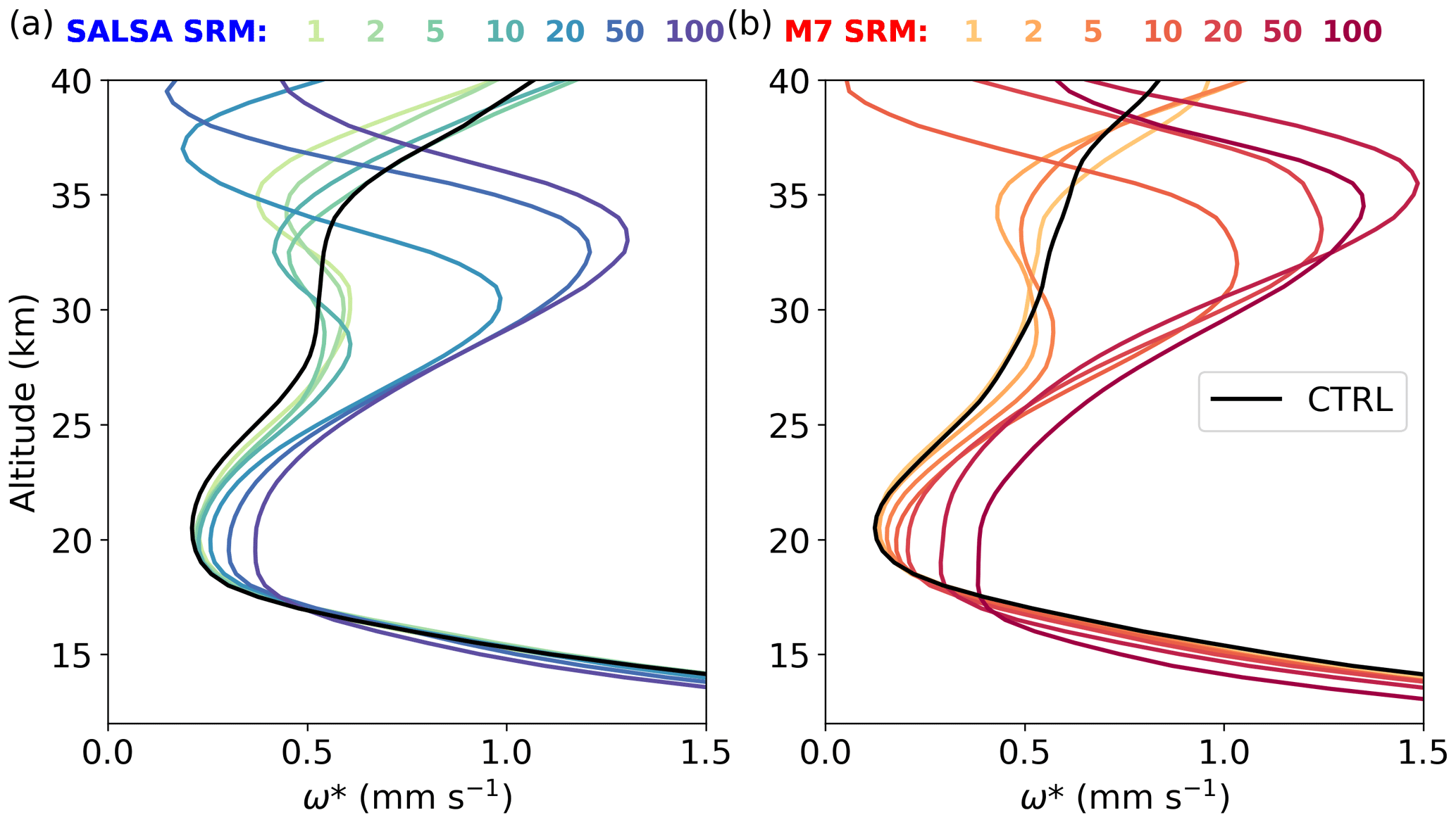
Figure 11Residual vertical velocity in the tropics (10∘ N–10∘ S) for different injection rates in simulations with (a) SALSA and (b) M7.
As the tropical stratosphere warms, it changes the dynamics of the atmosphere: for instance, it leads to a stronger vertical advection that further strengthens the lofting of aerosols and makes the lifetime of aerosols longer. Figure 11 shows the residual vertical velocity (ω∗) between 10∘ N and 10∘ S in the Baseline scenarios with the different injection rates. Higher injection rates cause stronger warming which further strengthens ω∗ at the injection altitude (20–22 km) and even up to 30 km altitude. As expected, based on the stronger warming seen in M7 than in SALSA (Fig. 10), the increase in the updraught velocity is generally higher in M7. In the case of a 100 Tg (S) yr−1 injection rate in M7, the increase in ω∗ was 360 % at an altitude of 20 km. However, it should be noted that the profiles of ω∗ in the CTRL simulation without SAI were significantly different between SALSA and M7. This is discussed later in this section. While residual vertical velocity increases above the tropopause, the residual vertical velocity decreases with the simulated injection rate in the upper troposphere. This reduction is larger in M7 than in SALSA, and the simulation of a 100 Tg(S)yr−1 injection rate with M7 showed a 35 % lower residual vertical velocity at 15 km altitude compared with the CTRL simulation. One interesting feature is also seen at altitudes higher than 25 km, where the ω∗ changes drastically when the injection rate is large enough. In SALSA, this takes place in injection scenarios higher than 10 Tg (S) yr−1, whereas it occurs at a much lower injection threshold of 5 Tg (S) yr−1 in M7. Below the above-mentioned injection rate, ω∗ is roughly 0.5 mm s−1 at 30 km altitude, and for a larger injection rate, ω∗ is larger than 1.0 mm s−1. Tropical ω∗ for different injection scenarios compared with the Baseline scenario with injection rates of 5 and 50 Tg (S) yr−1 are shown in Fig. S12.
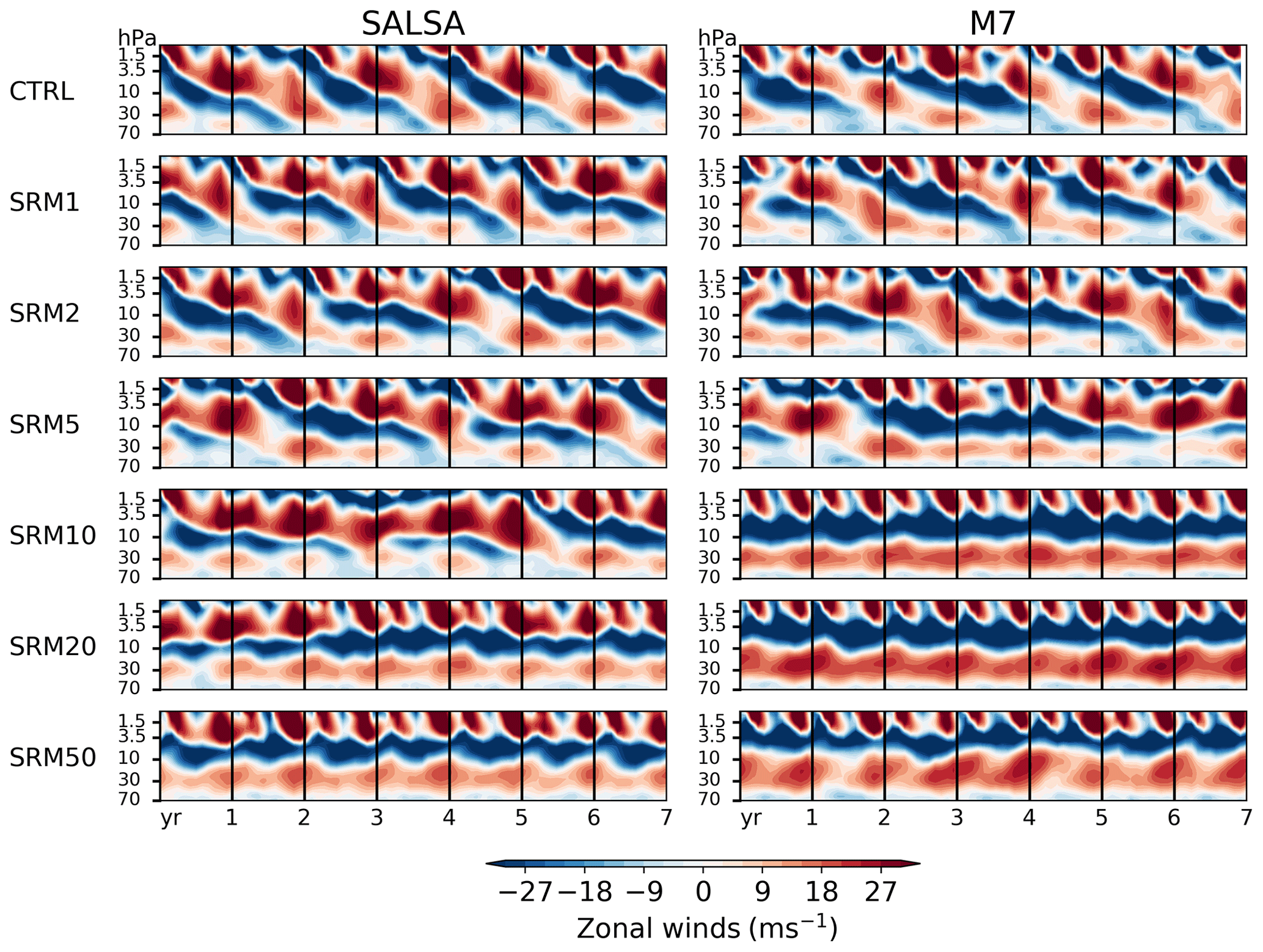
Figure 12Zonal mean zonal wind (m s−1) at the Equator for the CTRL simulation and stratospheric sulfur injection with different injection rates. The SALSA results are shown in the left panels, and the M7 results are shown in the right panels.
Changes in the zonal and meridional wind patterns in December–January–February and June–July–August are shown in the Supplement (Figs. S13–S16). The zonal wind increase in the tropics is stronger with higher injection rates in M7 than in SALSA. In some cases, the meridional wind pattern anomalies in the SAI scenarios have different signs between SALSA and M7. Stratospheric sulfur injections have also been shown to, for example, strengthen the stratospheric polar vortex (Visioni et al., 2020a). It is expected that these changes are also sensitive to the aerosol model and the injection strategies. However, a more detailed analysis of this is beyond of the scope of this study.
One consequence of the warming of the tropical stratosphere in the case of equatorial injections is the slowing down of the quasi-biennial oscillation (QBO), and if the injection rate is high enough, the QBO can be shut down completely (Niemeier and Schmidt, 2017). This statement was also supported by our simulations. As can be seen in Fig. 12, the QBO slowed down with increasing injection rate. Based on the M7 simulations, the shutting down of the QBO occurs at injection rates higher than 10 Tg (S) yr−1, whereas a rate of more than 20 Tg (S) yr−1 is required in SALSA. This corresponds to stratospheric temperature anomalies compared with the CTRL scenario, which were the same magnitude in those two simulations. In addition, following the shutting down of the QBO, the westerly phase of the QBO in the lower stratosphere is stronger and reaches higher altitudes in M7 compared with the results of the corresponding injection magnitude in SALSA. In M7, stratospheric heating due to stratospheric aerosols was stronger than in SALSA; thus, the QBO slowed down and vanished at lower injection rates. A similar difference in the impacts on the QBO between climate models has been seen in Niemeier et al. (2020), caused by a difference in the residual vertical velocity between models and different heating rates in the lower stratosphere. It is also likely that the difference in the responses in the QBO between models in this study is not fully caused by aerosol microphysics.
As Figs. 11 and 12 show, the residual vertical velocity and QBO were different between the aerosol schemes even without the stratospheric sulfur injections despite the fact that the same atmospheric model was used. In the CTRL simulations, M7 has a much longer period of the QBO than in SALSA, and it is overestimated compared with the 28 months seen in observations (Naujokat, 1986). Although the same atmospheric model was used, different tuning parameters were used depending on the aerosol microphysical model, and the atmospheric temperature is not consistent between models, even in the CTRL simulation (Fig. S17). Based on test simulations, which were performed before the actual simulations of this study, the tuning of the model had a significant impact on the QBO. In addition, even though the aerosol concentration in the stratosphere is low in the CTRL simulations, the tropospheric aerosols and the following indirect cloud impacts are different between the aerosol schemes used. In the M7 simulations, modes were modified to represent stratospheric aerosols more accurately by narrowing the standard deviation of the coarse mode and changing the threshold radius when aerosols from the accumulation mode are transferred to the coarse mode. A disadvantage of this modified set-up is that large tropospheric aerosols are probably not represented as well as in the standard set-up. Differences in the tropospheric aerosols and tuning parameters led to a warmer upper troposphere and lower stratosphere in SALSA than in M7, as seen in Fig. S17. Thus, the residual vertical wind (Fig. 11), the zonal and meridional wind patterns, and the QBO are different between SALSA and M7 in the CTRL simulations. This will also lead to some bias in the atmospheric circulation in the studied SAI scenarios between the models.
Franke et al. (2021) and Kravitz et al. (2019) have shown that the response of the QBO to sulfur injections depends on the location of injections. In Franke et al. (2021), where sulfur was injected into two grid boxes located at 30∘ N and 30∘ S, and in Kravitz et al. (2019), where sulfur was injected at four different latitudes based on a feedback algorithm, the QBO was not significantly affected, even with 25 Tg (S)−1 injections. The QBO in our sensitivity scenarios is shown in Fig. S18. The scenarios studied here included injections at the Equator. However, in the Seasonal scenario, the injection region varied, and sulfur was injected at the Equator during only a part of the year. In this case, sulfur injection did not have a significant impact on the QBO, even if 50 Tg (S)−1 was injected in the SALSA simulation. The results of the corresponding scenario with M7 showed that the QBO was prolonged with an injection rate of 20 Tg (S)−1 and shut down with an injection rate of 50 Tg (S)−1. In all the other scenarios, the QBO vanished with a 50 Tg (S)−1 injection rate, and it vanished in most scenarios with an injection rate of 20 Tg (S)−1 in both models. In the Low, High and Wide scenarios, the QBO did not fully disappear in the case of a 20 Tg (S)−1 injection rate with SALSA, but the cycle were significantly prolonged.
Here, we have systematically studied different spatio-temporal injection strategies with different magnitudes (2–100 Tg (S) yr−1) of sulfur injections using both the sectional (SALSA) and modal (M7) aerosol schemes in ECHAM-HAMMOZ. These simulations showed significant differences in the SW and LW radiative forcing, the size of the aerosols, and the lifetime of sulfur between the different injection strategies. In addition, modelled results were very sensitive to which microphysics model was used in the simulations. While both models show a sublinear increase in the global mean net radiative forcing as a function of the amount of sulfur injected due to increases in the size of aerosols, the net radiative forcing of SAI was 88 %–154 % higher based on simulation with SALSA than with M7. This large difference was also present when the SW and LW radiative responses between models were compared individually. While SW radiative forcing was 45 %–85 % higher (more negative) in SALSA than in M7 with the corresponding injection rate, the LW radiative forcing was 33 %–67 % larger in M7.
We identified two main factors that were causing different responses between models: (1) the numerical methods for describing the competitive processes of new particle formation and condensation inside the injection regime and (2) a local minimum in the aerosol number size distribution between two largest modes, caused by repartitioning of particles between the modes in the model, which coincidences with the optimal particle size for backscattering. In the stratosphere, new particle formation by nucleation is fed by continuous injections. However, there are already pre-existing particles from the preceding injections to which injected sulfur can condense. Thus, there is competition between these two processes for available sulfuric acid gas. In SALSA, sulfuric acid tends to form new particles rather than condensing on the pre-existing ones, whereas the opposite is true in the M7 simulations. Simulations with M7 showed that continuous injections and condensation increased the size of the largest (coarse) mode. However, due to the set-up for the repartitioning of particles between modes, this did not allow the second-largest mode to grow, creating a gap in the particle size distribution between the two largest modes. This gap coincided with the particle size range that would be optimal to scatter radiation.
There are several factors that support a sectional model over a modal model for stratospheric aerosol simulations, despite the fact that the modal scheme is significantly computationally faster than the sectional scheme (simulations with M7 were 60 % faster than SALSA). First of all, tropospheric and stratospheric aerosols require different configurations for modes; thus, studying the aerosols from both regions in the same simulations is not recommended. In addition, even though only stratospheric aerosols are studied, the tropospheric aerosols, which were not well represented by a configuration designed for stratospheric aerosols, can indirectly affect stratospheric aerosols. In SAI simulations, especially in the case of continuous injections, the size distribution inside the injection region does not have a clear multimodal structure in the sectional model simulations except for the lowest injection rates of 1–2 Tg (S) yr−1 (Figs. 5 and A3; English et al., 2012; Kleinschmitt et al., 2018). This is probably because there is available H2SO4 gas for particles to grow by condensation, and particles are not accumulating to certain size classes by coagulation. This kind of size distribution cannot be represented by four modes, and the problem culminates in the fact that there is a persistent gap between the two largest modes in this study. One option could be to use more modes, but the computational benefits compared with sectional schemes would then become smaller. In the standard set-up of M7, the (largest) coarse-mode width is 2.0 instead of 1.2 (which is used here). This would make the gap between the two largest modes smaller. However, in the case of stratospheric sulfur injections or a large volcanic eruption, a wider coarse-mode width leads to a tail of large particles. This causes an overestimation of the effective radius of the coarse mode, increases the sedimentation velocity and reduces the residence time of aerosols in the stratosphere, which is the reason why a different set-up is used for stratospheric aerosols. One option could be to increase the mode widths of the Aitken and accumulation modes. However, the number concentrations of these modes are typically higher; therefore, widening of the modes can lead to a situation in which the widened mode would cover the adjacent larger mode. It is also good to keep in mind that the partitioning of sulfuric acid to the particle phase due to nucleation over condensation was suspiciously large in SALSA, and the model produced a significantly larger net total radiative forcing than in studies such as Kleinschmitt et, al. (2018), where simulations were done with the sectional model. Thus, even though there was not as clear a shortcoming as the gap between modes in M7, there is a need to analyse the individual microphysical processes and to understand the differences between the results of different sectional models.
Overall, differences in the results between the two microphysical models reveal significant uncertainties related to stratospheric sulfur injections. Thus, there is a need for better tools to analyse aerosol microphysical processes under stratospheric conditions when using continuous injections and to improve the aerosol–climate models. A comparison with the observations of large volcanic eruptions (e.g Mt. Pinatubo) does not necessarily offer a true picture of the model performance when using continuous injections, as there is not as much competition with respect to nucleation and condensation in the case of volcanic eruptions, where a large amount of sulfate erupts abruptly to a relatively particle-free stratosphere. It is also good to keep in mind that sulfur would most plausibly be injected into the stratosphere by aircraft (Smith and Wagner, 2018). In these simulations with the climate model, the injected SO2 is instantly mixed in the model grid box which is a few hundred square kilometres in size. Thus, the microphysics that takes place inside of plume after injection is not captured by ECHAM-HAMMOZ or by aerosol–climate models in general. In addition, the time step of climate models might be too long for aerosol microphysical processes which can cause strong bias, for example, where sulfuric acid concentrations are high and new particle formation and condensation are resolved simultaneously.
Shortcomings and uncertainties in microphysics will further lead to large uncertainties in estimating the possible climate impacts of stratospheric sulfur injection or, for example, in estimations of how much sulfur is required to achieve a certain climate target. To offer some perspective, compensating for all radiative forcing in the Representative Concentration Pathway (RCP) 2.6 from the pre-industrial period to the end of this century (2.6 W m−2) using stratospheric sulfur injections would require an approximate 3.7 Tg (S) yr−1 injection based on the results of SALSA, whereas 15 Tg (S) yr−1 would be required to achieve this based on M7. The difference is even more significant in extreme cases where the radiation imbalance in the RCP8.5 scenario (8.5 W m−2) would be compensated for by SAI. In this case, the estimation of required sulfur is either 22 Tg (S) yr−1 or over 100 Tg (S) yr−1 depending on the microphysical model. These differences between the model results can also have a significant impact on uncertainties related to the global mean precipitation. Larger LW absorption in M7 compared with SALSA might translate to a significant reduction in the global mean precipitation, which has been shown to be negatively correlated with absorbed radiation (Laakso et al., 2020). Lower net radiative forcing in M7 means that more sulfur should be injected to get the same cooling impact as in SALSA, which means even stronger absorption of LW radiation and a decrease in the global precipitation. This will be studied further in Part 2.
We also simulated different stratospheric sulfur injection strategies with both microphysical models. These scenarios were simulated with 2, 5, 20 and 50 Tg (S) yr−1 injection rates. We studied how choices of injecting to narrow vs. wide latitude bands, high vs. low altitude, into one grid box vs. a band over longitudes, and temporal differences between injection strategies (pulsed and seasonally changed) affect the radiative forcing of SAI and if the results are consistent between the models.
Differences in all-sky radiative forcing of the most efficient injection strategy compared with the least efficient strategy were 33 %–42 % higher depending on the injection rate based on SALSA. Simulations with M7 showed even larger variation in radiative forcing, and all-sky radiative forcing in the most efficient SAI scenario was 48 %–116 % higher than in the least efficient simulated scenario. However, simulations of the Point scenario with high injection rates (> 20 Tg (S)−1) simulated with M7 showed an increase in the sulfate lifetime with increasing injection rate. This differs from all other scenarios and the Point scenario simulated with SALSA. If the Point scenario is not taken into account, the most efficient SAI scenario in M7 simulations exhibited a forcing that was 76 % higher than the least efficient scenario. Based on results from both models, the three most efficient scenarios were Point, Pulse-Jan-Jul and Seasonal. Common to all of these scenarios was that instead of stable injections to a band across all longitudes, injections were done either by injecting only to one model grid box, suspending injection for 5 months before the next injection period or the changing injection area seasonally.
Because the forcing efficiency decreases with the injection rate, the injection strategy is important, especially for a high injection rate. As an example, based on M7 simulations, a 20 Tg (S) yr−1 injection rate using a seasonal injection strategy instead of equatorial injections (Baseline) would enhance the global mean all-sky radiative forcing by 53 %. Achieving the same enhancement using equatorial injections would require a 42 Tg (S) yr−1 injection rate instead of 20 Tg (S) yr−1.
Our Baseline scenario, where sulfur was injected continuously between 10∘ N and 10∘ S at 20–22 km altitude, resulted in, depending on the injection rate, the smallest or the second-smallest net radiative forcing of all of the studied injection strategies. Only the Narrow injection strategy (injecting into a two-grid-box-wide band over the Equator) led to a smaller radiative forcing when simulated with M7 and 5 and 20 Tg (S) yr−1 injection rates. In SALSA, the Wide injection scenario was the least efficient when less than 20 Tg (S) yr−1 was injected. Based on the simulations, injecting sulfur into lower altitudes (18–20 km) was more efficient than injecting sulfur at a 20–22 km altitude in both models with the exception of the simulation with M7 for a 50 Tg (S) yr−1 injection rate.
If the studied injection strategies are ranked based on their global mean radiative forcing, there are not large differences in the order irrespective of whether SALSA or M7 results were used. Injecting twice per year in 1-month periods was the most efficient injection strategy based on SALSA and M7 with the exception of a 50 Tg (S) yr−1 injection when simulated with M7, where the continuous injection into one grid box resulted in an exceptionally large impact. Generally, relative differences in the global mean radiative forcings between the different injection strategies were larger when simulated with M7 than with SALSA. Overall, the results from both models indicated that injection over an area where large aerosols from preceding injections already exist would lead to higher condensation on the existing particles or that new particles would coagulate with the existing ones, which reduces the efficiency of SAI.
The zonal mean radiative forcings' dependence on the injection strategy was qualitatively similar between the models. Equatorial injections in our Baseline scenario resulted in maximum zonal forcing over the tropics. This relative disproportion of radiative forcing between low and high latitudes was increased with higher injection rates. Comparing this with the Baseline scenario, injecting sulfur into a narrow band or to one model grid box increased the radiative forcing over the tropics, as expected. On the other hand, injecting sulfur at a lower altitude, into a wider band over the Equator or changing the injection area seasonally led to reduced radiative forcing over tropics compared with our Baseline scenario. For example, compared with the Baseline scenarios, changing the injection area seasonally led to 29 % larger all-sky radiative forcing over non-tropics in case of an injection rate of 5 Tg (S) yr−1 in SALSA, and this value was 75 % in M7. In the tropics, the corresponding changes were 13 % smaller and 12 % larger all-sky radiative forcing with SALSA and M7 respectively. Several studies have shown that offsetting the mean GHG warming with uniform SRM or equatorial injections can lead to overcooling of the tropics and warming at high latitudes. This could be prevented by seasonally varying the sulfur injections and without any trade-off in the total radiative forcing, as the net all-sky radiative forcing of the seasonally changing injection strategy was one of the most efficient of the studied scenarios. Moreover, as it also reduced LW absorption compared with the Baseline scenario, it would also lead to a smaller reduction in global mean precipitation (Laakso et al., 2020).
We also studied dynamical changes in the stratosphere. As M7 produced larger aerosols and higher absorption of LW radiation, warming in the stratosphere was stronger in the M7 simulations than in SALSA. Thus, the increase in the residual vertical velocity was larger and the slowing down of the QBO was more significant in M7 than in simulations with the corresponding injection rate with SALSA. In our Baseline scenario, the QBO vanished with injection rates higher than 10 Tg (S) yr−1 based on simulation with M7, whereas more than 20 Tg (S) yr−1 was required to shut down the QBO in the simulation with SALSA. Based on SALSA simulations, the Seasonal scenario did not have a significant impact on the slowing down of the QBO even with 50 Tg (S) yr−1 injections.
Most SAI studies have focused on equatorial injections as the baseline case. Injection between 10∘ N and 10∘ S was also chosen as the injection scenario in the G6sulfur GeoMIP experiment (Kravitz et al., 2015). As the results here show, there are several factors than indicate that equatorial injection should not be used as baseline scenario: (1) it is less efficient than most of the studied alternative injection scenarios, (2) the resulting radiative forcing is concentrated in the tropics and (3) the warming of tropical stratosphere leads to a slowing down or vanishing QBO, which could be avoided by some other injection strategies such as varying the injection area seasonally. However, providing a suggestion for an alternative baseline scenario for following studies or, for example, the next possible GeoMIP experiments is not straightforward, as SAI can be used to meet various different climate targets, and none of the injection strategies can be optimized to meet all of the targets. In addition, there were, for example, some changes in the mutual ranking in global mean forcing between studied scenarios, depending on injection rate. This is true especially when considering injection rates that can be considered “more realistic” (< 10 Tg (S) yr−1). In scenarios like G6sulfur, where the injection rate varies, the most logical scenario for lower injection rates may not be the same as for higher injection rates. As this study shows, the radiative forcing of certain injection strategies is also significantly dependent on the aerosol model. Thus, there is a need for a model intercomparison project using aerosol–climate models to simulate various SAI scenarios.
Here, the simulations were done with a model configuration with a fixed sea surface temperature, and the objective was to analyse the impact of injection strategies and aerosol microphysical models on radiative forcing. The next step is to study how these radiative forcings translate to climate impacts (i.e changes in global and regional temperature and especially precipitation) and if these responses are dependent on the climate model. This will be studied in Part 2.
Our analyses in this study showed that model responses on stratospheric aerosol injection were significantly different between the sectional aerosol model SALSA and modal aerosol scheme M7. Based on Fig. 4, this difference between the models is partly caused by how models solve the competition between new particle formation and condensation inside or near the injection regime. While injected sulfur tends to mainly form new particles in SALSA, sulfate condensates on pre-existing particles in M7. To study the role of these differences on radiative forcing and particle size distribution we performed additional simulations where competition between nucleation and condensation were made consistent between the models. This was done by switching nucleation off and emitting 25 % of injected sulfur as 3 nm primary particles while the rest of the sulfur was injected as SO2. Simulations were run for the Baseline scenario with 2, 5, 20 and 50 Tg (S) yr−1 injections. By standardizing the competition between nucleation and condensation in SALSA and M7, the global mean SW radiative forcing, net radiative forcing and especially stratospheric sulfur burden between models are closer to each other than in the original set-up (see Fig. A1). However, differences in the LW radiative forcing between models were slightly increased, and the SW response was still significantly larger in SALSA than in M7. Thus, the different treatment of the competition between nucleation and condensation only partly explains the responses between models. This is interesting, especially because the zonal mean effective radius of stratospheric aerosols is consistent in these sensitivity simulation between models (See Fig. A2). However, a closer look at the aerosol size distribution inside the injection regime shows that even though the effective radius was consistent between models, the size distribution was not. Generally, size distributions in simulations where nucleation is replaced by injecting 3 nm primary aerosols are relatively similar to those in the original simulations, excluding the two smallest modes in the M7 simulations (Fig. A3). The median size of the nucleation (smallest) mode is larger, the number of Aitken mode (second smallest) aerosols is significantly higher and the median size is smaller than in the original simulations. Because of this, the effective radius of stratospheric aerosols is significantly smaller. However, the aerosols in the nucleation and Aitken modes do not have a notable impact on the radiation. As Fig. A3 shows, the two largest modes, accumulation and coarse, are relatively similar to those in the original simulations. There is still a large gap between these two modes, which is located at the size range of the largest backscattering efficiency. In addition, the number of coarse-mode aerosols is even higher than with the original set-up which explains the larger LW radiative forcing.
Overall, these simulations show that different radiative responses between the models mainly originated from the representation of aerosols (sectional vs. modal), which has been discussed in Sect. 3.2. In addition, this analysis shows that the effective radius is not always a representative measure of the size distribution and that radiative impacts can be significantly different, even in case of consistent effective radius.

Figure A1Global mean (a) short-wave, (b) long-wave and (c) total radiative forcing as well as (d) the stratospheric sulfate burden as a function of injection rate. M7 results are shown in red, and SALSA results are shown in blue. The lighter dashed lines correspond to original simulations, and the darker solid lines represent the corresponding simulations without nucleation.
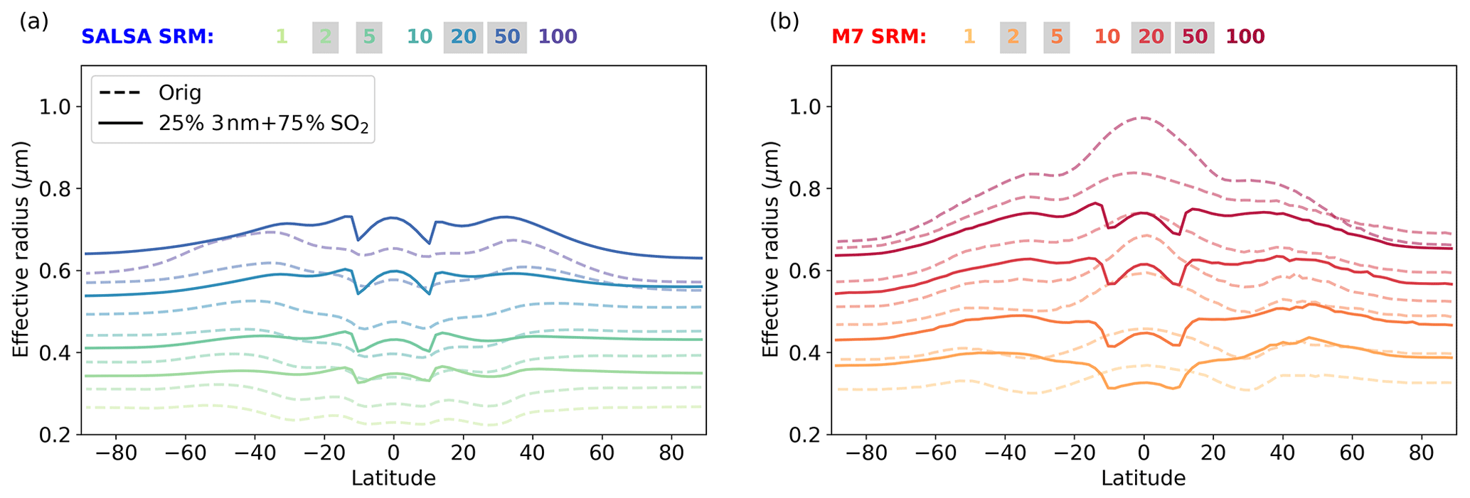
Figure A2Zonal mean effective radius of stratospheric aerosols for different magnitudes of sulfur injections simulated with (a) SALSA and (b) M7. The lighter dashed lines correspond to the original simulations, and the darker solid lines represent the corresponding simulations without nucleation.
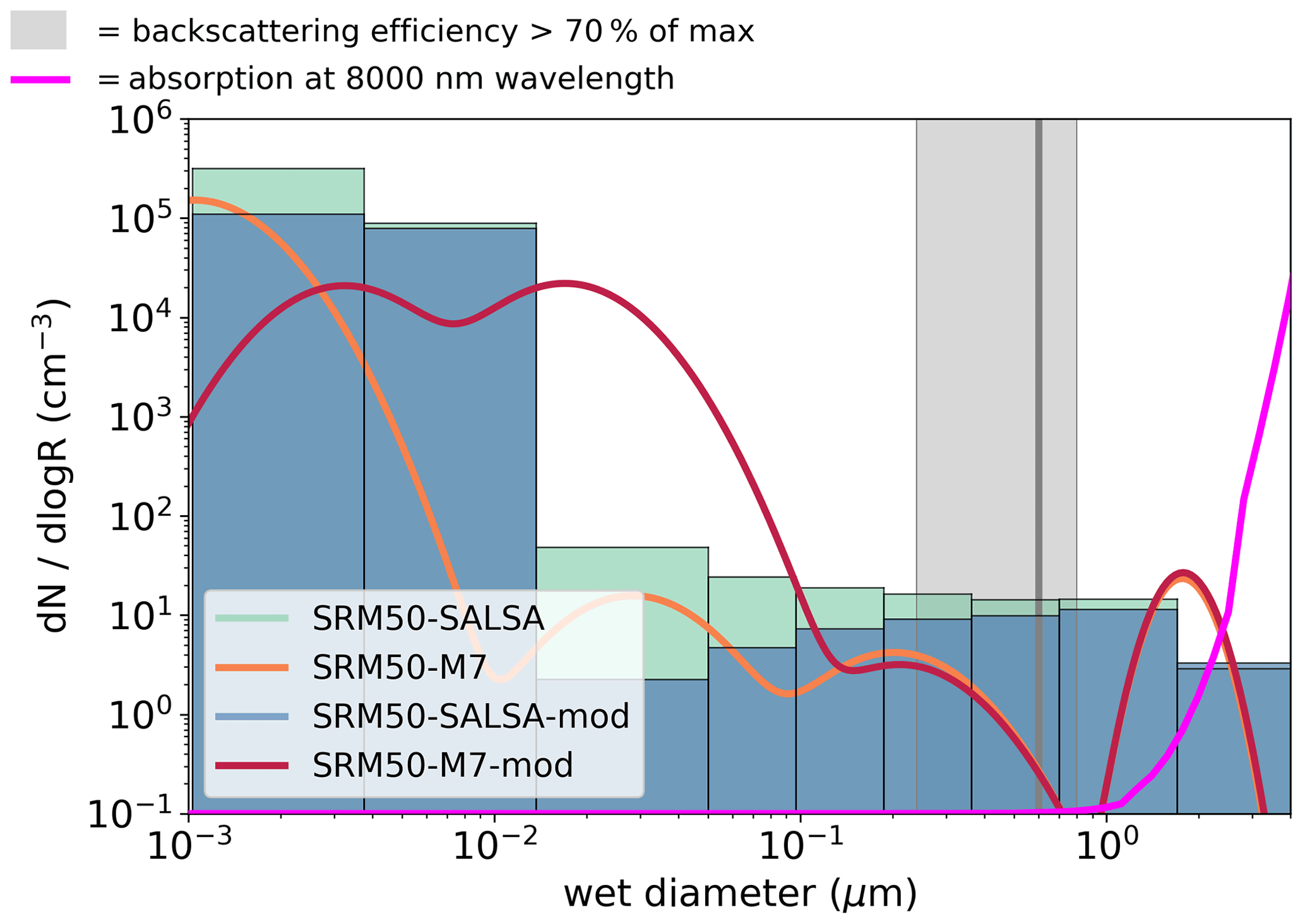
Figure A3The aerosol number size distribution inside of the injection regime in scenario SRM50 simulated with M7 and SALSA in the original simulations and in simulations where the nucleation is replaced by injecting 25 % of sulfur mass as 3 nm primary particles. The grey line shows the size of the maximum backscattering, and shaded area indicates the radius where aerosol backscattering is 70 % of the maximum from Dykema et al. (2016). The magenta line shows the dependence of absorption at an 8000 nm wavelength on the (dry) size of the sulfate aerosols, based on the radiation module of SALSA.
The data from the model simulations and the implemented model codes are available from the authors upon request.
The supplement related to this article is available online at: https://doi.org/10.5194/acp-22-93-2022-supplement.
AL designed the research, performed the experiments, carried out the analysis and prepared the paper. All authors contributed ideas, participated in the interpretation and discussion of the results, and contributed to writing the paper.
The contact author has declared that neither they nor their co-authors have any competing interests.
Publisher's note: Copernicus Publications remains neutral with regard to jurisdictional claims in published maps and institutional affiliations.
This article is part of the special issue “Resolving uncertainties in solar geoengineering through multi-model and large-ensemble simulations (ACP/ESD inter-journal SI)”. It is not associated with a conference.
The ECHAM-HAMMOZ model is developed by a consortium composed of ETHZ, the Max-Planck-Institut für Meteorologie, Forschungszentrum Jülich, the University of Oxford, and the Finnish Meteorological Institute; it is managed by the Center of Climate Systems Modeling (C2SM) at ETHZ.
This research has been supported by the Tiina and Antti Herlin Foundation (grant nos. 20190014 and 20200003). Ulrike Niemeier obtained support from the German DFG-funded Research Unit VollImpact (FOR2820, grant no. 398006378).
This paper was edited by Anja Schmidt and reviewed by Ben Kravitz and Peter Irvine.
Aswathy, V. N., Boucher, O., Quaas, M., Niemeier, U., Muri, H., Mülmenstädt, J., and Quaas, J.: Climate extremes in multi-model simulations of stratospheric aerosol and marine cloud brightening climate engineering, Atmos. Chem. Phys., 15, 9593–9610, https://doi.org/10.5194/acp-15-9593-2015, 2015. a
Bergman, T., Kerminen, V.-M., Korhonen, H., Lehtinen, K. J., Makkonen, R., Arola, A., Mielonen, T., Romakkaniemi, S., Kulmala, M., and Kokkola, H.: Evaluation of the sectional aerosol microphysics module SALSA implementation in ECHAM5-HAM aerosol-climate model, Geosci. Model Dev., 5, 845–868, https://doi.org/10.5194/gmd-5-845-2012, 2012. a
Caldeira, K., Bala, G., and Cao, L.: The Science of Geoengineering, Annu. Rev. Earth Pl. Sc., 41, 231–256, https://doi.org/10.1146/annurev-earth-042711-105548, 2013. a
Chen, J.-P. and Lamb, D.: Simulation of Cloud Microphysical and Chemical Processes Using a Multicomponent Framework. Part I: Description of the Microphysical Model, J. Atmos. Sci., 51, 2613–2630, https://doi.org/10.1175/1520-0469(1994)051<2613:SOCMAC>2.0.CO;2, 1994. a
Dykema, J. A., Keith, D. W., and Keutsch, F. N.: Improved aerosol radiative properties as a foundation for solar geoengineering risk assessment, Geophys. Res. Lett., 43, 7758–7766, https://doi.org/10.1002/2016GL069258, 2016. a, b, c, d
English, J. M., Toon, O. B., and Mills, M. J.: Microphysical simulations of sulfur burdens from stratospheric sulfur geoengineering, Atmos. Chem. Phys., 12, 4775–4793, https://doi.org/10.5194/acp-12-4775-2012, 2012. a, b
English, J. M., Toon, O. B., and Mills, M. J.: Microphysical simulations of large volcanic eruptions: Pinatubo and Toba, J. Geophys. Res.-Atmos., 118, 1880–1895, https://doi.org/10.1002/jgrd.50196, 2013. a
Franke, H., Niemeier, U., and Visioni, D.: Differences in the quasi-biennial oscillation response to stratospheric aerosol modification depending on injection strategy and species, Atmos. Chem. Phys., 21, 8615–8635, https://doi.org/10.5194/acp-21-8615-2021, 2021. a, b
Heckendorn, P., Weisenstein, D., Fueglistaler, S., Luo, B. P., Rozanov, E., Schraner, M., Thomason, L. W., and Peter, T.: The impact of geoengineering aerosols on stratospheric temperature and ozone, Environ. Res. Lett., 4, 045108, https://doi.org/10.1088/1748-9326/4/4/045108, 2009. a, b, c, d, e, f
Jacobson, M. Z.: Analysis of aerosol interactions with numerical techniques for solving coagulation, nucleation, condensation, dissolution, and reversible chemistry among multiple size distributions, J. Geophys. Res.-Atmos., 107, AAC 2-1–AAC 2-23, https://doi.org/10.1029/2001JD002044, 2002. a
Jones, A. C., Haywood, J. M., and Jones, A.: Climatic impacts of stratospheric geoengineering with sulfate, black carbon and titania injection, Atmos. Chem. Phys., 16, 2843–2862, https://doi.org/10.5194/acp-16-2843-2016, 2016. a
Kerminen, V.-M. and Kulmala, M.: Analytical formulae connecting the “real” and the “apparent” nucleation rate and the nuclei number concentration for atmospheric nucleation events, J. Aerosol Sci., 33, 609–622, https://doi.org/10.1016/S0021-8502(01)00194-X, 2002. a
Kleinschmitt, C., Boucher, O., and Platt, U.: Sensitivity of the radiative forcing by stratospheric sulfur geoengineering to the amount and strategy of the SO2injection studied with the LMDZ-S3A model, Atmos. Chem. Phys., 18, 2769–2786, https://doi.org/10.5194/acp-18-2769-2018, 2018. a, b, c, d, e, f, g, h, i, j, k, l, m
Kokkola, H., Hommel, R., Kazil, J., Niemeier, U., Partanen, A.-I., Feichter, J., and Timmreck, C.: Aerosol microphysics modules in the framework of the ECHAM5 climate model – intercomparison under stratospheric conditions, Geosci. Model Dev., 2, 97–112, https://doi.org/10.5194/gmd-2-97-2009, 2009. a, b, c, d, e, f
Kokkola, H., Kühn, T., Laakso, A., Bergman, T., Lehtinen, K. E. J., Mielonen, T., Arola, A., Stadtler, S., Korhonen, H., Ferrachat, S., Lohmann, U., Neubauer, D., Tegen, I., Siegenthaler-Le Drian, C., Schultz, M. G., Bey, I., Stier, P., Daskalakis, N., Heald, C. L., and Romakkaniemi, S.: SALSA2.0: The sectional aerosol module of the aerosol–chemistry–climate model ECHAM6.3.0-HAM2.3-MOZ1.0, Geosci. Model Dev., 11, 3833–3863, https://doi.org/10.5194/gmd-11-3833-2018, 2018. a, b, c, d, e, f
Kravitz, B., Robock, A., Tilmes, S., Boucher, O., English, J. M., Irvine, P. J., Jones, A., Lawrence, M. G., MacCracken, M., Muri, H., Moore, J. C., Niemeier, U., Phipps, S. J., Sillmann, J., Storelvmo, T., Wang, H., and Watanabe, S.: The Geoengineering Model Intercomparison Project Phase 6 (GeoMIP6): simulation design and preliminary results, Geosci. Model Dev., 8, 3379–3392, https://doi.org/10.5194/gmd-8-3379-2015, 2015. a
Kravitz, B., MacMartin, D. G., Wang, H., and Rasch, P. J.: Geoengineering as a design problem, Earth Syst. Dynam., 7, 469–497, https://doi.org/10.5194/esd-7-469-2016, 2016. a
Kravitz, B., MacMartin, D. G., Mills, M. J., Richter, J. H., Tilmes, S., Lamarque, J.-F., Tribbia, J. J., and Vitt, F.: First Simulations of Designing Stratospheric Sulfate Aerosol Geoengineering to Meet Multiple Simultaneous Climate Objectives, J. Geophys. Res.-Atmos., 122, 12616–12634, https://doi.org/10.1002/2017JD026874, 2017. a
Kravitz, B., MacMartin, D. G., Tilmes, S., Richter, J. H., Mills, M. J., Cheng, W., Dagon, K., Glanville, A. S., Lamarque, J.-F., Simpson, I. R., Tribbia, J., and Vitt, F.: Comparing Surface and Stratospheric Impacts of Geoengineering With Different SO2 Injection Strategies, J. Geophys. Res.-Atmos., 124, 7900–7918, https://doi.org/10.1029/2019JD030329, 2019. a, b
Kravitz, B., MacMartin, D. G., Visioni, D., Boucher, O., Cole, J. N. S., Haywood, J., Jones, A., Lurton, T., Nabat, P., Niemeier, U., Robock, A., Séférian, R., and Tilmes, S.: Comparing different generations of idealized solar geoengineering simulations in the Geoengineering Model Intercomparison Project (GeoMIP), Atmos. Chem. Phys., 21, 4231–4247, https://doi.org/10.5194/acp-21-4231-2021, 2021. a
Laakso, A., Kokkola, H., Partanen, A.-I., Niemeier, U., Timmreck, C., Lehtinen, K. E. J., Hakkarainen, H., and Korhonen, H.: Radiative and climate impacts of a large volcanic eruption during stratospheric sulfur geoengineering, Atmos. Chem. Phys., 16, 305–323, https://doi.org/10.5194/acp-16-305-2016, 2016. a, b, c, d
Laakso, A., Korhonen, H., Romakkaniemi, S., and Kokkola, H.: Radiative and climate effects of stratospheric sulfur geoengineering using seasonally varying injection areas, Atmos. Chem. Phys., 17, 6957–6974, https://doi.org/10.5194/acp-17-6957-2017, 2017. a, b, c, d, e, f, g, h, i, j
Laakso, A., Snyder, P. K., Liess, S., Partanen, A.-I., and Millet, D. B.: Differing precipitation response between solar radiation management and carbon dioxide removal due to fast and slow components, Earth Syst. Dynam., 11, 415–434, https://doi.org/10.5194/esd-11-415-2020, 2020. a, b, c, d, e, f
McCusker, K. E., Battisti, D. S., and Bitz, C. M.: The Climate Response to Stratospheric Sulfate Injections and Implications for Addressing Climate Emergencies, J. Climate, 25, 3096–3116, https://doi.org/10.1175/JCLI-D-11-00183.1, 2012. a
Mills, M. J., Richter, J. H., Tilmes, S., Kravitz, B., MacMartin, D. G., Glanville, A. A., Tribbia, J. J., Lamarque, J.-F., Vitt, F., Schmidt, A., Gettelman, A., Hannay, C., Bacmeister, J. T., and Kinnison, D. E.: Radiative and Chemical Response to Interactive Stratospheric Sulfate Aerosols in Fully Coupled CESM1(WACCM), J. Geophys. Res.-Atmos., 122, 13061–13078, https://doi.org/10.1002/2017JD027006, 2017. a, b
Naujokat, B.: An Update of the Observed Quasi-Biennial Oscillation of the Stratospheric Winds over the Tropics, J. Atmos. Sci., 43, 1873–1877, https://doi.org/10.1175/1520-0469(1986)043<1873:AUOTOQ>2.0.CO;2, 1986. a
Niemeier, U. and Schmidt, H.: Changing transport processes in the stratosphere by radiative heating of sulfate aerosols, Atmos. Chem. Phys., 17, 14871–14886, https://doi.org/10.5194/acp-17-14871-2017, 2017. a, b, c, d, e, f, g
Niemeier, U. and Timmreck, C.: What is the limit of climate engineering by stratospheric injection of SO2?, Atmos. Chem. Phys., 15, 9129–9141, https://doi.org/10.5194/acp-15-9129-2015, 2015. a, b, c, d, e, f, g, h, i, j, k, l, m, n, o, p, q, r, s
Niemeier, U., Timmreck, C., Graf, H.-F., Kinne, S., Rast, S., and Self, S.: Initial fate of fine ash and sulfur from large volcanic eruptions, Atmos. Chem. Phys., 9, 9043–9057, https://doi.org/10.5194/acp-9-9043-2009, 2009. a, b, c
Niemeier, U., Schmidt, H., and Timmreck, C.: The dependency of geoengineered sulfate aerosol on the emission strategy, Atmos. Sci. Lett., 12, 189–194, https://doi.org/10.1002/asl.304, 2011. a, b, c, d, e, f, g
Niemeier, U., Richter, J. H., and Tilmes, S.: Differing responses of the quasi-biennial oscillation to artificial SO2 injections in two global models, Atmos. Chem. Phys., 20, 8975–8987, https://doi.org/10.5194/acp-20-8975-2020, 2020. a
Niemeier, U., Riede, F., and Timmreck, C.: Simulation of ash clouds after a Laacher See-type eruption, Clim. Past, 17, 633–652, https://doi.org/10.5194/cp-17-633-2021, 2021. a
Pierce, J. R., Weisenstein, D. K., Heckendorn, P., Peter, T., and Keith, D. W.: Efficient formation of stratospheric aerosol for climate engineering by emission of condensible vapor from aircraft, Geophys. Res. Lett., 37, L18805, https://doi.org/10.1029/2010GL043975, 2010. a, b
Richter, J. H., Tilmes, S., Mills, M. J., Tribbia, J. J., Kravitz, B., MacMartin, D. G., Vitt, F., and Lamarque, J.-F.: Stratospheric Dynamical Response and Ozone Feedbacks in the Presence of SO2 Injections, J. Geophys. Res.-Atmos., 122, 12557–12573, https://doi.org/10.1002/2017JD026912, 2017. a
Schultz, M. G., Stadtler, S., Schröder, S., Taraborrelli, D., Franco, B., Krefting, J., Henrot, A., Ferrachat, S., Lohmann, U., Neubauer, D., Siegenthaler-Le Drian, C., Wahl, S., Kokkola, H., Kühn, T., Rast, S., Schmidt, H., Stier, P., Kinnison, D., Tyndall, G. S., Orlando, J. J., and Wespes, C.: The chemistry–climate model ECHAM6.3-HAM2.3-MOZ1.0, Geosci. Model Dev., 11, 1695–1723, https://doi.org/10.5194/gmd-11-1695-2018, 2018. a
Smith, W. and Wagner, G.: Stratospheric aerosol injection tactics and costs in the first 15 years of deployment, Environ. Res. Lett., 13, 124001, https://doi.org/10.1088/1748-9326/aae98d, 2018. a
Stevens, B., Giorgetta, M., Esch, M., Mauritsen, T., Crueger, T., Rast, S., Salzmann, M., Schmidt, H., Bader, J., Block, K., Brokopf, R., Fast, I., Kinne, S., Kornblueh, L., Lohmann, U., Pincus, R., Reichler, T., and Roeckner, E.: Atmospheric component of the MPI-M Earth System Model: ECHAM6, J. Adv. Model. Earth Sy., 5, 146–172, https://doi.org/10.1002/jame.20015, 2013. a
Sukhodolov, T., Sheng, J.-X., Feinberg, A., Luo, B.-P., Peter, T., Revell, L., Stenke, A., Weisenstein, D. K., and Rozanov, E.: Stratospheric aerosol evolution after Pinatubo simulated with a coupled size-resolved aerosol–chemistry–climate model, SOCOL-AERv1.0, Geosci. Model Dev., 11, 2633–2647, https://doi.org/10.5194/gmd-11-2633-2018, 2018. a
Tegen, I., Neubauer, D., Ferrachat, S., Siegenthaler-Le Drian, C., Bey, I., Schutgens, N., Stier, P., Watson-Parris, D., Stanelle, T., Schmidt, H., Rast, S., Kokkola, H., Schultz, M., Schroeder, S., Daskalakis, N., Barthel, S., Heinold, B., and Lohmann, U.: The global aerosol–climate model ECHAM6.3–HAM2.3 – Part 1: Aerosol evaluation, Geosci. Model Dev., 12, 1643–1677, https://doi.org/10.5194/gmd-12-1643-2019, 2019. a, b, c
Tilmes, S., Fasullo, J., Lamarque, J.-F., Marsh, D. R., Mills, M., Alterskjær, K., Muri, H., Kristjánsson, J. E., Boucher, O., Schulz, M., Cole, J. N. S., Curry, C. L., Jones, A., Haywood, J., Irvine, P. J., Ji, D., Moore, J. C., Karam, D. B., Kravitz, B., Rasch, P. J., Singh, B., Yoon, J.-H., Niemeier, U., Schmidt, H., Robock, A., Yang, S., and Watanabe, S.: The hydrological impact of geoengineering in the Geoengineering Model Intercomparison Project (GeoMIP), J. Geophys. Res.-Atmos., 118, 11036–11058, https://doi.org/10.1002/jgrd.50868, 2013. a
Tilmes, S., Richter, J. H., Kravitz, B., MacMartin, D. G., Mills, M. J., Simpson, I. R., Glanville, A. S., Fasullo, J. T., Phillips, A. S., Lamarque, J.-F., Tribbia, J., Edwards, J., Mickelson, S., and Ghosh, S.: CESM1(WACCM) Stratospheric Aerosol Geoengineering Large Ensemble Project, B. Am. Meteorol. Soc., 99, 2361–2371, https://doi.org/10.1175/BAMS-D-17-0267.1, 2018a. a
Tilmes, S., Richter, J. H., Mills, M. J., Kravitz, B., MacMartin, D. G., Garcia, R. R., Kinnison, D. E., Lamarque, J.-F., Tribbia, J., and Vitt, F.: Effects of Different Stratospheric SO2 Injection Altitudes on Stratospheric Chemistry and Dynamics, J. Geophys. Res.-Atmos., 123, 4654–4673, https://doi.org/10.1002/2017JD028146, 2018b. a, b
Toohey, M., Krüger, K., Niemeier, U., and Timmreck, C.: The influence of eruption season on the global aerosol evolution and radiative impact of tropical volcanic eruptions, Atmos. Chem. Phys., 11, 12351–12367, https://doi.org/10.5194/acp-11-12351-2011, 2011. a
Vattioni, S., Weisenstein, D., Keith, D., Feinberg, A., Peter, T., and Stenke, A.: Exploring accumulation-mode H2SO4 versus SO2 stratospheric sulfate geoengineering in a sectional aerosol–chemistry–climate model, Atmos. Chem. Phys., 19, 4877–4897, https://doi.org/10.5194/acp-19-4877-2019, 2019. a, b, c, d, e, f
Vignati, E., Wilson, J., and Stier, P.: M7: An efficient size-resolved aerosol microphysics module for large-scale aerosol transport models, J. Geophys. Res., 109, D22202, https://doi.org/10.1029/2003JD004485, 2004. a
Visioni, D., MacMartin, D. G., Kravitz, B., Tilmes, S., Mills, M. J., Richter, J. H., and Boudreau, M. P.: Seasonal Injection Strategies for Stratospheric Aerosol Geoengineering, Geophys. Res. Lett., 46, 7790–7799, https://doi.org/10.1029/2019GL083680, 2019. a, b
Visioni, D., MacMartin, D. G., Kravitz, B., Lee, W., Simpson, I. R., and Richter, J. H.: Reduced Poleward Transport Due to Stratospheric Heating Under Stratospheric Aerosols Geoengineering, Geophys. Res. Lett., 47, e2020GL089470, https://doi.org/10.1029/2020GL089470, 2020a. a, b, c
Visioni, D., Slessarev, E., MacMartin, D. G., Mahowald, N. M., Goodale, C. L., and Xia, L.: What goes up must come down: impacts of deposition in a sulfate geoengineering scenario, Environ. Res. Lett., 15, 094063, https://doi.org/10.1088/1748-9326/ab94eb, 2020b. a
Visioni, D., MacMartin, D. G., and Kravitz, B.: Is Turning Down the Sun a Good Proxy for Stratospheric Sulfate Geoengineering?, J. Geophys. Res.-Atmos., 126, e2020JD033952, https://doi.org/10.1029/2020JD033952, 2021. a
Wan, H., Rasch, P. J., Zhang, K., Kazil, J., and Leung, L. R.: Numerical issues associated with compensating and competing processes in climate models: an example from ECHAM-HAM, Geosci. Model Dev., 6, 861–874, https://doi.org/10.5194/gmd-6-861-2013, 2013. a, b
Young, K. C.: A Numerical Simulation of Wintertime, Orographic Precipitation: Part I. Description of Model Microphysics and Numerical Techniques, J. Atmos. Sci., 31, 1735–1748, https://doi.org/10.1175/1520-0469(1974)031<1735:ANSOWO>2.0.CO;2, 1974. a
Yu, X., Moore, J. C., Cui, X., Rinke, A., Ji, D., Kravitz, B., and Yoon, J.-H.: Impacts, effectiveness and regional inequalities of the GeoMIP G1 to G4 solar radiation management scenarios, Global Planet. Change, 129, 10–22, https://doi.org/10.1016/j.gloplacha.2015.02.010, 2015. a
Zhang, K., O'Donnell, D., Kazil, J., Stier, P., Kinne, S., Lohmann, U., Ferrachat, S., Croft, B., Quaas, J., Wan, H., Rast, S., and Feichter, J.: The global aerosol-climate model ECHAM-HAM, version 2: sensitivity to improvements in process representations, Atmos. Chem. Phys., 12, 8911–8949, https://doi.org/10.5194/acp-12-8911-2012, 2012. a