Estimated regional CO₂ flux and uncertainty based on an ensemble of atmospheric CO₂ inversions

Global and regional sources and sinks of carbon across the earth's surface have been studied extensively using atmospheric carbon dioxide (CO₂) observations and atmospheric chemistry-transport model (ACTM) simulations (top-down/inversion method). However, the uncertainties in the regional flux distributions remain unconstrained due to the lack of high-quality measurements, uncertainties in model simulations, and representation of data and flux errors in the inversion systems. Here, we assess the representation of data and flux errors using a suite of 16 inversion cases derived from a single transport model (MIROC4-ACTM) but different sets of a priori (bottom-up) terrestrial biosphere and oceanic fluxes, as well as prior flux and observational data uncertainties (50 sites) to estimate CO₂ fluxes for 84 regions over the period 2000–2020. The inversion ensembles provide a mean flux field that is consistent with the global CO₂ growth rate, land and ocean sink partitioning of −2.9 ± 0.3 (± 1σ uncertainty on the ensemble mean) and −1.6 ± 0.2 PgC yr⁻¹, respectively, for the period 2011–2020 (without riverine export correction), offsetting about 22 %–33 % and 16 %–18 % of global fossil fuel CO₂ emissions. The rivers carry about 0.6 PgC yr⁻¹ of land sink into the deep ocean, and thus the effective land and ocean partitioning is −2.3 ± 0.3 and −2.2 ± 0.3, respectively. Aggregated fluxes for 15 land regions compare reasonably well with the best estimations for the 2000s (∼ 2000–2009), given by the REgional Carbon Cycle Assessment and Processes (RECCAP), and all regions appeared as a carbon sink over 2011–2020. Interannual variability and seasonal cycle in CO₂ fluxes are more consistently derived for two distinct prior fluxes when a greater degree of freedom (increased prior flux uncertainty) is given to the inversion system. We have further evaluated the inversion fluxes using meridional CO₂ distributions from independent (not used in the inversions) aircraft and surface measurements, suggesting that the ensemble mean flux (model–observation mean ± 1σ standard deviation = −0.3 ± 3 ppm) is best suited for global and regional CO₂ flux budgets than an individual inversion (model–observation 1σ standard deviation = −0.35 ± 3.3 ppm). Using the ensemble mean fluxes and uncertainties for 15 land and 11 ocean regions at 5-year intervals, we show promise in the capability to track flux changes toward supporting the ongoing and future CO₂ emission mitigation policies.

1 Introduction

Carbon dioxide is the most important anthropogenic greenhouse gas in the Earth's atmosphere. Due to human influences, e.g., fossil fuel consumption and cement production (FFC), the concentration of atmospheric CO₂ increased (by 38 %) from 289.9 ± 3.3 ppm in 1850–1900 to 398.8 ± 7.3 ppm in 2010–2019, with the fastest growth in the past 5 decades (Canadell et al., 2021). To limit global warming below 1.5^∘C by 2100, as per the Paris Agreement, a drastic and sustained reduction in CO₂ emissions from anthropogenic activities is recommended in the IPCC's sixth assessment report (AR6). The IPCC AR6 Working Group 1 estimated remaining carbon budgets (starting from 1 January 2020) for limiting global warming to 1.5, 1.7, and 2.0 ^∘C as 140, 230, and 370 PgC, respectively, based on the 50th percentile of the transient climate response to cumulative emissions of carbon dioxide (TCRE) (Canadell et al., 2021). With the present FFC emissions of about 10 PgC yr⁻¹ (Jones et al., 2021), the remaining carbon budget will be consumed within decades.

The sinks on the land and ocean constitute a major component of nature-based solutions to mitigate the rise in CO₂ concentration, as discussed in the IPCC AR6 (Canadell et al., 2021). During 2010–2019, the CO₂ emissions from human activities (average rate of 10.9 ± 0.9 PgC yr⁻¹) were distributed between three Earth system components: 46 % accumulated in the atmosphere (5.1 ± 0.02 PgC yr⁻¹), 23 % was taken up by the ocean (2.5 ± 0.6 PgC yr⁻¹), and 31 % was stored by vegetation in terrestrial ecosystems (3.4 ± 0.9 PgC yr⁻¹) (Table 5.1 in Canadell et al., 2021). Large uncertainties persist for the total global land and ocean sink partitioning in the IPCC assessment, up to about 25 % of the global total land and ocean sinks. The uncertainty in land and ocean sink partitioning of about 1 PgC yr⁻¹ in the IPCC AR6 is based on the annual carbon budget of the Global Carbon Project (GCP) (Friedlingstein et al., 2020). One of the impediments to making policy for CO₂ emission reduction is poor knowledge of the regional sources and sinks of carbon in Earth's disturbed and undisturbed ecosystems on land and in the ocean (Kondo et al., 2020). To estimate regional CO₂ sources and sinks, the country-scale socio-economic statistics, field studies, and remote sensing of the earth's environment are most commonly used (bottom-up or inventory estimation), which often suffers from reliable data or regular data updates (Ito, 2019; Jones et al., 2021). In the other method (top-down estimations), observations and model simulations of atmospheric concentrations are used to estimate CO₂ sources and sinks in the terrestrial biosphere and the oceans (Peylin et al., 2013).

Top-down inverse models estimate residual natural or non-FFC CO₂ fluxes from land and ocean regions because inversion calculations do not explicitly optimize the FFC emissions; i.e., the FFC emissions are not revised, but the a priori land and ocean sinks are revised. When different sources of FFC emissions are used in inversions, post-inversion corrections are applied for comparison between inversions (Peylin et al., 2013; Thompson et al., 2016). More recently, the inverse model inter-comparison experiments use prescribed FFC emissions, e.g., the global carbon project (Friedlingstein et al., 2020) or the OCO-2 flux intercomparison (Crowell et al., 2019), to avoid the post-inversion correction. However, the impacts of biases in FFC emissions on inversion estimated CO₂ fluxes remained relatively unexplored (Saeki and Patra, 2017). The FFC emission biases affect the region of FFC emission and the regions linked closely by atmospheric transport. This is because (1) the prior flux uncertainties set for each of the inversion regions may not be sufficient to allow for fully compensatory correction by inversion, (2) the model transport biases could move FFC emission signals slowly or quickly from the source region, and (3) emission signal goes undetected within the region when there are not enough measurement sites in the source region of biased FFC. Most FFC emission inventories are based on the data available from the International Energy Agency (IEA) and British Petroleum and mainly differ in spatial distribution within a given country (Crippa et al., 2020; Jones et al., 2021; Oda et al., 2018).

The GCP annual updates of inversions provide a metric for evaluating inversions using independent measurements, mainly from aircraft campaigns (e.g., Friedlingstein et al., 2020). Evaluation of predicted fluxes from model–data differences may not be straightforward due to the underlying assumptions of a flux inversion system, e.g., for flux correlation lengths or the radius of influence for the measurements, observational data uncertainty, prior flux uncertainty (Baker et al., 2010; Chevallier et al., 2007; van der Laan-Luijkx et al., 2017; Miyazaki et al., 2011; Niwa et al., 2017; Rödenbeck et al., 2003), while the data assimilation system will fit the model concentrations to the observed values. For example, a model–observation difference within ± 1 ppm and/or vertical concentration gradient simulation within 1σ standard deviation of the observed gradient resulted in more than 1 PgC yr⁻¹ flux differences between models at regional or sub-hemispheric scales (Gaubert et al., 2019; Stephens et al., 2007; Thompson et al., 2016). Another way of improving our knowledge about uncertainties in regional flux estimations is to employ multiple types of datasets from both bottom-up and top-down modeling systems (Ciais et al., 2021; Kondo et al., 2020), which we have adapted here for checking the regional inversion fluxes, in addition to the GCP-like evaluation using independent aircraft data.

The uncertainties in the regional fluxes mainly arise from prior flux distribution and seasonality, selection of observational network and data uncertainty, transport model resolution leading to site-representation error, and uncertainties arising from parameterization of transport processes (Basu et al., 2018; Patra et al., 2005a; Philip et al., 2019; Qu et al., 2021; Wang et al., 2018). The uncertainties associated with the subcontinental-scale CO₂ fluxes are often much greater than the interannual and interdecadal flux changes in non-FFC sectors, which allows us to make a better assessment of the changes in regional CO₂ fluxes compared to knowledge gained in regional flux magnitudes (Baker et al., 2006; Gurney et al., 2008; Patra et al., 2005a, b; Peylin et al., 2013; Rayner et al., 2008; Rödenbeck et al., 2003). Typically, a multi-model assessment of flux estimation uncertainties is performed by collecting inversions from different transport models, e.g., in TransCom (Baker et al., 2006; Gurney et al., 2008; Peylin et al., 2013), for inversions using GOSAT measurements (Houweling et al., 2015) or for inversions using OCO-2 (Crowell et al., 2019; Peiro et al., 2022). Such intercomparisons used single inversions from different modeling groups and provided the range in total CO₂ flux uncertainty due to the choices of prior fluxes distribution, prior flux uncertainty, observational data uncertainty, and the model transport uncertainties.

Here we show an ensemble-based inversion approach based on different choices of prior flux uncertainties and representation of measurement data uncertainties, using a single chemistry-transport model (JAMSTEC's MIROC4-ACTM). The details of the MIROC4-ACTM, observed and model data processing, inversion setup are given in Sect. 2, followed by the results and discussion in Sect. 3. The fluxes and uncertainties are presented at regional and global scales, along with their validation using inversion-independent observations. Although the inversions are performed for the period 1998–2020, results are discussed mainly for the 2 most recent decades (2001–2010 and 2011–2020), with the only exception of comparing land–ocean flux partitioning with the IPCC AR6. Conclusions are given in Sect. 4.

2 Materials and method

2.1 JAMSTEC's MIROC version 4 atmospheric chemistry-transport model (MIROC4-ACTM)

The Model for Interdisciplinary Research on Climate version 4 (MIROC4; Watanabe et al., 2008) atmospheric general circulation model (AGCM)-based chemistry-transport model (referred to as MIROC4-ACTM; Patra et al., 2018) is used for the forward simulations of CO₂. The MIROC earth system model is developed at JAMSTEC in collaboration with the University of Tokyo and the National Institute of Environmental Studies (NIES) (Kawamiya et al., 2020). Simulations of long-lived gases (CO₂, CH₄, N₂O, SF₆) in the atmosphere are performed at a horizontal resolution of T42 spectral truncations (∼ $\mathrm{2.8}{}^{\circ }\times \mathrm{2.8}{}^{\circ }$ latitude–longitude grid) with 67 vertical hybrid-pressure layers between the Earth's surface and 0.0128 hPa (∼ 80 km) (Bisht et al., 2021; Chandra et al., 2021; Patra et al., 2017, 2018). The simulated horizontal winds (U, V) and temperature (T) are nudged with the Japan Meteorological Agency Reanalysis data product (JRA-55; Kobayashi et al., 2015) at the altitude range of ∼ 980–0.018 hPa for better representation of the atmospheric transport at synoptic and seasonal timescales. An accurate representation of transport is essential for performing inverse model calculation by minimizing biases in horizontal and vertical gradients in the simulated tracer fields. We tested the large-scale interhemispheric transport and Brewer–Dobson circulation in the MIROC4-ACTM using the SF₆ simulations in the troposphere and the CO₂-derived age of air in the troposphere and stratosphere (Bisht et al., 2021; Patra et al., 2018). A close match between observed and modeled SF₆ and photochemically inert CO₂ vertical gradient in the troposphere and lower stratosphere manifests the accurate transport in the MIROC4-ACTM. Reasonably good model transport in MIROC4-ACTM enables us to use any mismatch between observation and simulations to estimate the land and oceanic fluxes using the inverse modeling technique (details in Sect. 2.4).

2.2 A priori CO₂ simulations

We simulated CO₂ tracers corresponding to the FFC (CO${}_{\mathrm{2}}^{\mathrm{ff}}$), land biosphere fluxes (CO${}_{\mathrm{2}}^{\mathrm{lnd}}$), fire emissions (CO${}_{\mathrm{2}}^{\mathrm{fire}}$), and ocean exchanges (CO${}_{\mathrm{2}}^{\mathrm{ocn}}$) from different sets of prior (bottom-up) emissions (Table 1). CO${}_{\mathrm{2}}^{\mathrm{ff}}$ is simulated using the gridded fossil fuel emission dataset (GridFED; Jones et al., 2021). CO${}_{\mathrm{2}}^{\mathrm{lnd}}$ tracers are simulated using two sets of terrestrial biosphere fluxes from the Carnegie-Ames-Stanford Approach (CASA) biogeochemical model (Randerson et al., 1997) and Vegetation Integrative Simulator for Trace Gases (VISIT) (Ito, 2019). The CASA fluxes are annually balanced, seasonally varying flux due to terrestrial photosynthesis and respiration, while the VISIT simulation accounts for CO₂ fertilization (increasing photosynthesis due to rising atmospheric CO₂), LUC (perturbation on terrestrial carbon budget due to land-use change), and climate variability. VISIT simulates a large land sink on the net (Table 1). The CASA and VISIT monthly-mean fluxes are downscaled to 3-hourly time intervals by redistributing respiration and gross primary production (Olsen and Randerson, 2004) using JRA-55 meteorology, i.e., 2 m air temperature and incoming solar radiation at the earth surface (Table 1). Monthly-mean fire emissions are used from GFEDv4.1s (van der Werf et al., 2017) for simulating the CO${}_{\mathrm{2}}^{\mathrm{fire}}$ tracer. Sea–air CO₂ fluxes are taken from an upscaling model of shipboard measurements of pCO₂ (referred to here as TT09: Takahashi et al., 2009), and an empirical model of the Japan Meteorological Agency (JMA; Iida et al., 2021) for simulating CO${}_{\mathrm{2}}^{\mathrm{ocn}}$ tracers. The seasonal cycle for TT09 sea–air exchange flux is stationary, like that of the CASA, over the analysis period, while the JMA oceanic CO₂ fluxes vary interannually, as in the case of VISIT. The model and prior fluxes' details are given in Table 1.

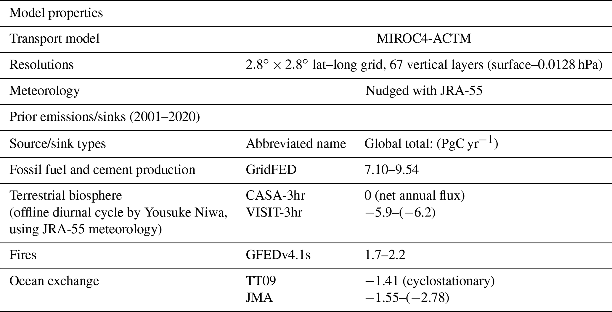
Table 1 Transport model setup and a priori CO₂ emissions used for simulating the atmospheric CO₂ concentrations. The range in prior fluxes (2001–2020) is also given in petagrams of carbon per year (PgC yr⁻¹) for the study period.

We prepare two cases of prior CO₂ simulations by adding the CO₂ flux tracers in different combinations as follows:

$$\begin{array}{}\text{(1a)}& {\displaystyle }\begin{array}{rl}\mathrm{gc}\mathrm{3}\mathrm{t}& ={{\mathrm{CO}}_{\mathrm{2}}}^{\mathrm{ff}}\left(\mathrm{GridFED}\right)+{{\mathrm{CO}}_{\mathrm{2}}}^{\mathrm{lnd}}\left(\text{CASA-3hr}\right)\\ & +{{\mathrm{CO}}_{\mathrm{2}}}^{\mathrm{ocn}}\left(\mathrm{TT}\mathrm{09}\right)\end{array}\text{(1b)}& {\displaystyle }\begin{array}{rl}\mathrm{gvjf}& ={{\mathrm{CO}}_{\mathrm{2}}}^{\mathrm{ff}}\left(\mathrm{GridFED}\right)+{{\mathrm{CO}}_{\mathrm{2}}}^{\mathrm{lnd}}\left(\text{VISIT-3hr}\right)\\ & +{{\mathrm{CO}}_{\mathrm{2}}}^{\mathrm{ocn}}\left(\mathrm{JMA}\right)+{{\mathrm{CO}}_{\mathrm{2}}}^{\mathrm{fire}}.\end{array}\end{array}$$

The gvjf case includes all the known interannual variability in land fluxes due to climate as simulated by VISIT and ocean fluxes by JMA. In contrast, the gc3t case has no information on interannual variability in land and ocean fluxes and the annual land sink. These two a priori flux cases are designed to evaluate the strength of MIROC4-ACTM inversions to derive fluxes consistently (or the lack of it) given the information on CO₂ measurements from a network of sites and the statistics of prior flux uncertainty (PFU) and model data uncertainty (MDU).

2.3 Atmospheric data selection and curve fitting

We used CO₂ observations from 50 measurement sites (marked in Fig. 1) for the inverse modeling (Supplement Table S1). Observations are taken from GML/NOAA (38 sites), CSIRO (four sites), LSCE/IPSL (one site), SIO (two sites), SAWS (one site), ECCC (one site), and JMA (three sites). Data until 2019 are taken from obspack_co2_1_GLOBALVIEWplus_v6.1_2021-03-01 (Schuldt et al., 2021), and JMA data are taken from WDCGG. Extension to obspack_co2_1_GLOBALVIEWplus_v6.1 for 2020 is compiled from GML/NOAA (https://gml.noaa.gov/aftp/data/trace_gases/co2/flask/, last access: 12 July 2022) and WDCGG (https://gaw.kishou.go.jp/, last access: 12 July 2022) websites as appropriate. We further extended the 2020 values into 2021 based on the growth rate determined for January–March observed at Minamitorishima (MNM) as available on the WDCGG (the results of 2021 will not be used in any analysis and will be treated as the spin-down year of inversion). The model simulations are sampled at the observation time and the grid point nearest to the observation location at hourly intervals. We selected the sites where the temporal data gaps are minimum, no more than 6-month data gaps at a stretch for the inversion period (1999–2020). These temporal data gaps (1–6 months) are filled using the curve fitting method based on the digital filtering technique (Nakazawa et al., 1997). We fit the measured and simulated time series at daily-weekly time intervals with six harmonics (extracts the sinusoidal component, i.e., seasonal cycle) and Butterworth digital filter with a cutoff length of 24 months (determines the long-term trends).

2.4 Inverse method

Inverse analysis of atmospheric CO₂ helps to link the atmospheric observations to carbon fluxes from land and ocean. We use a time-dependent Bayesian inversion system, initially developed by Rayner et al. (1999). The inversion formalism specifies prior estimates of both the fluxes and their uncertainty (called prior flux uncertainty (PFU)) and optimizes fluxes over 54 land and 30 ocean regions (Fig. 1) by minimizing the difference between the CO₂ mixing ratios simulated by the MIROC4-ACTM and observed at 50 measurement sites for 1998–2021. We exclude the first 2 years and last year of inversion from our analysis period (2000–2020) to avoid the edge effect.

In the Bayesian inversion, when the relation between model parameters and data parameters is linear (d=Js), the misfit function (χ²) is constructed as (Rayner et al., 2008; Tarantola, 2005)

$$\begin{array}{}\text{(2)}& \begin{array}{rl}{\mathit{\chi }}^{\mathrm{2}}& ={\displaystyle \frac{\mathrm{1}}{\mathrm{2}}}[{\left(\mathit{s}-{\mathit{s}}_{\mathrm{0}}\right)}^T\mathbf{C}{\left({\mathit{s}}_{\mathrm{0}}\right)}^{-\mathrm{1}}\left(\mathit{s}-{\mathit{s}}_{\mathrm{0}}\right)\\ & +{\left(\mathbf{J}\mathit{s}-\mathit{d}\right)}^T\mathbf{C}{\left(\mathit{d}\right)}^{-\mathrm{1}}\left(\mathbf{J}\mathit{s}-\mathit{d}\right)].\end{array}\end{array}$$

Assuming that the elements of C(d) are uncorrelated, the solutions for s and C(s) can then be written as

$$\begin{array}{}\text{(3)}& \begin{array}{rl}<\mathit{s}>=& {\mathit{s}}_{\mathrm{0}}+{\left({\mathbf{J}}^T\mathbf{C}{\left(\mathit{d}\right)}^{-\mathrm{1}}\mathbf{J}+\mathbf{C}{\left({\mathit{s}}_{\mathrm{0}}\right)}^{-\mathrm{1}}\right)}^{-\mathrm{1}}\\ & {\mathbf{J}}^T\mathbf{C}{\left(\mathit{d}\right)}^{-\mathrm{1}}\left({\mathit{d}}_{\mathrm{obs}}-{\mathit{d}}_{\mathrm{ACTM}}\right)\end{array}\end{array}$$

and posterior error covariance

$$\begin{array}{}\text{(4)}& \mathbf{C}\left(\mathit{s}\right)={\left({\mathbf{J}}^T\mathbf{C}{\left(\mathit{d}\right)}^{-\mathrm{1}}\mathbf{J}+\mathbf{C}{\left({\mathit{s}}_{\mathrm{0}}\right)}^{-\mathrm{1}}\right)}^{-\mathrm{1}},\end{array}$$

where s₀ is the prior source for the 84 regions and 288 months in 1998–2021, C(s₀) is the prior source error covariance matrix, d_obs is the measurement data at 50 sites for 288 months, and C(d) is the data error covariance matrix. d_ACTM(≈Js₀) is the forward model simulation time series using a priori fluxes, run continuously for the whole period of analysis and sampled at the time and locations of the individual measurement before calculating monthly means. J is the Jacobian matrix of sensitivities of observations with respect to s, calculated using simulations of unitary pulse sources for a month for the 84 basis regions and sampled at the 50 measurement sites. The unitary pulses are simulated for 4 years (1 month of emissions and 47 months of zero emissions) and originated for each month of year 2011 for all regions (84 regions × 12 months = 1008 tracers per year). One set of J matrix is reused for all years. The elements of J for later months are kept constant at the value of the 48th month. We have shown in Fig. S1 and associated text that the use of annually repeating J does not significantly affect the inversion results as the majority of the spatial and temporal flux variabilities are coming from the a priori flux, which are simulated using interannually varying meteorology. The elements in s are the optimized CO₂ fluxes (referred to as a posteriori or predicted flux) from 84 regions at monthly time intervals. The off-diagonal elements of C(s₀) are kept zero, assuming the a priori fluxes are uncorrelated to one another region or time. The correction fluxes (s−s₀ in Eq. 3) are primarily determined by the term (d_ACTM−d_obs), scaled by the data/flux uncertainty.

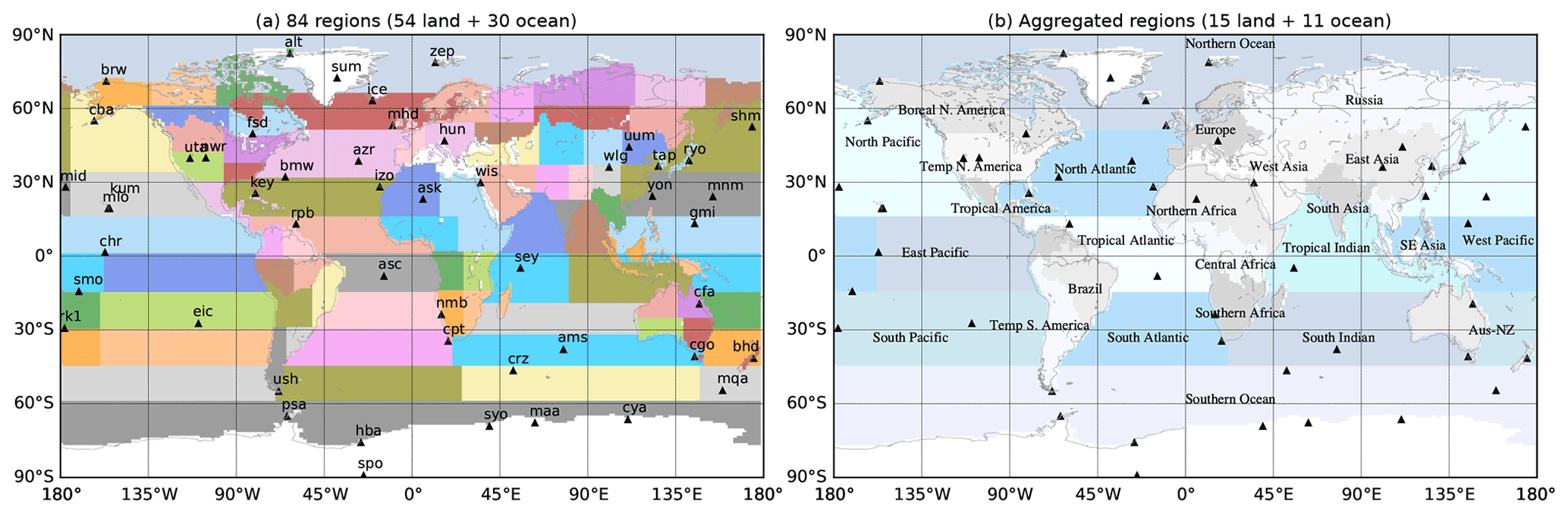
Figure 1 Divisions of 54 land and 30 ocean regions for inverse modeling and 50 observation sites (a). Panel (b) shows the analysis regions adopted in this study (15 land and 11 ocean), which are consistent with the boundaries of the RECCAP phase 2 (RECCAP2) land regions (Ciais et al., 2022) and TransCom ocean regions (Gurney et al., 2002).

The inversion settings based on the choice of a priori fluxes, MDU, and PFU are crucial for flux estimation. The MDU refers to the degree to which the predicted concentrations are required to be fitted by the inverse model. In addition to measurement precision, MDU incorporates the inability of coarse spatial-resolution global ACTMs to simulate the concentrations at the observation sites. PFU decides the degree of freedom or allowed flux adjustment for each of the 84 regions to match the atmospheric data. It determines to what extent the priors are relied upon to constrain the posterior flux estimates. To determine the robustness of our results, we have performed sensitivity analysis by varying PFU and MDU (Table 2). In the first approach, we assign uniformly 2 PgC yr⁻¹ uncertainty to each of the 54 land regions and 0.75 PgC yr⁻¹ to each of the 30 ocean regions (referred to as PFU = “ctl”). In the second approach, we assign the land uncertainty by scaling the regional total FLUXCOM gross primary productivity (GPP) (Jung et al., 2017), while the uncertainty for the ocean regions is kept at 0.5 PgC yr⁻¹. In this case, regional total GPPs were multiplied by 2, and the upper limit is set at 2 PgC yr⁻¹ (referred to as gpp_v2; PFUs varied from 0.2–2.0 PgC yr⁻¹). We construct two additional PFU cases (gpp_v3 and gpp_v4) by multiplying the regional total GPPs by a factor of 3 and 4, respectively, and the allowed range is set at 0.3–3.0 and 0.4–4.0 PgC yr⁻¹. The land PFUs varied as 0.4–3.0 and 0.6-4.0 PgC yr⁻¹ for the gpp_v3 and gpp_v4, respectively. The ocean PFUs were set at 0.75 PgC yr⁻¹ for gpp_v3 and 1.0 PgC yr⁻¹ for gpp_v4 (Table 2). Selection of a wide range of PFUs, in the range of 0.5–1.0 PgC yr⁻¹ for the ocean regions and 0.2–4.0 PgC yr⁻¹ for the land regions, allows us to understand the stability of the inversion system by assessing the range of a posteriori fluxes for aggregated subcontinental/basin regions or the land and ocean totals.

Table 2 List of 16 inversions based on the combinations of four different prior flux uncertainty (PFU) and model data uncertainty (MDU) cases. Each PFU and MDU combination case is run for the two prior flux distributions, (1) gc3t (GridFED + CASA-3hr + TT09) and (2) gvjf (GridFED + VISIT-3hr + JMA ocean + Fires − GFED). The abbreviation of inversion cases is arranged as PFU_MDU_Prior Flux.

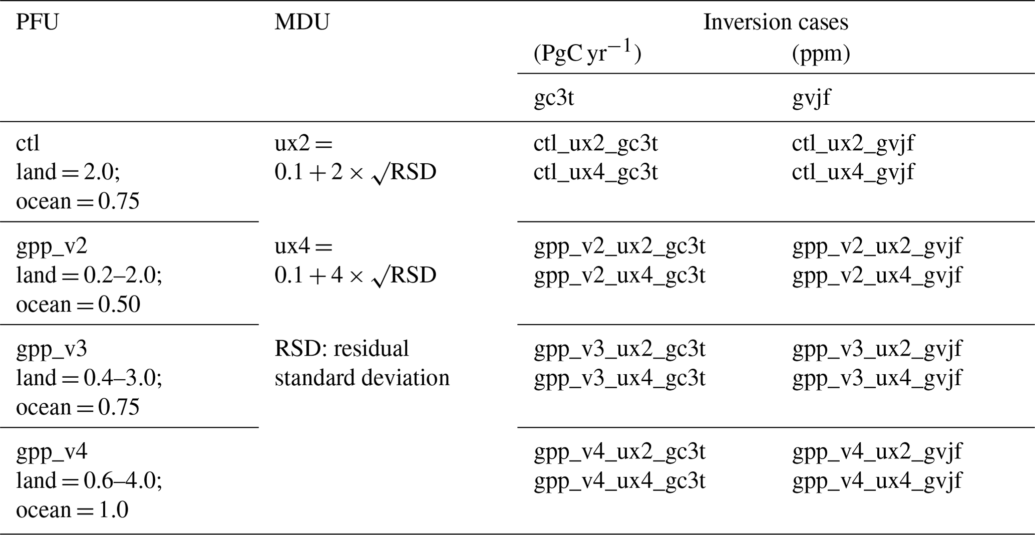
The monthly-mean residual standard deviation (RSD), from the difference between measured and fitted data, plus a constant value to account for the measurement accuracy, is used for monthly varying MDU at each station for inverse modeling calculations. The absolute magnitude of MDU is chosen in such a way that the estimated flux is optimized to the data only to an appropriate level commensurate with the ability of ACTM to model them. We prepared two MDU cases by multiplying the RSDs by a factor of 2 (referred to as “ux2”) and 4 (referred to as “ux4”) and added these to an estimated measurement uncertainty of 0.1 ppm. Based on different combinations of four PFU (ctl, gpp_v2, gpp_v3, gpp_v4), two MDU (ux2, ux4), and two prior flux cases (gc3t and gvjf), we run 16 sets of inversion cases (Table 2). Based on the inversions with multiple priors, PFUs and MDUs, we will present estimated mean/median fluxes and spread as 1σ standard deviations from 16 ensemble members.

Figure 2 shows the examples of simulated and observed time series of CO₂ (top row) and simulated–observed differences (bottom row) at two selected sites, Alert and Syowa. The results show faster (slower) CO₂ increase rates for the a priori-flux-simulated case gc3t (gvjf), mainly because of no land sink in CASA flux and stronger land sink in VISIT flux (broken red and purple lines, respectively). Using the mean of these two a priori flux scenarios, the prior CO₂ concentrations show a better match with the CO₂ growth rates (refer to the grey lines in the lower row; Fig. 2). Even after inversion, mild overestimation (underestimation) of the CO₂ growth rate for gc3t (gvjf) cases persisted, and by taking the ensemble mean inversion flux, the CO₂ growth rates are perfectly matched with the observations (Fig. 2), which is sometimes set as an evaluation metric for atmospheric CO₂ inversions (Friedlingstein et al., 2020).

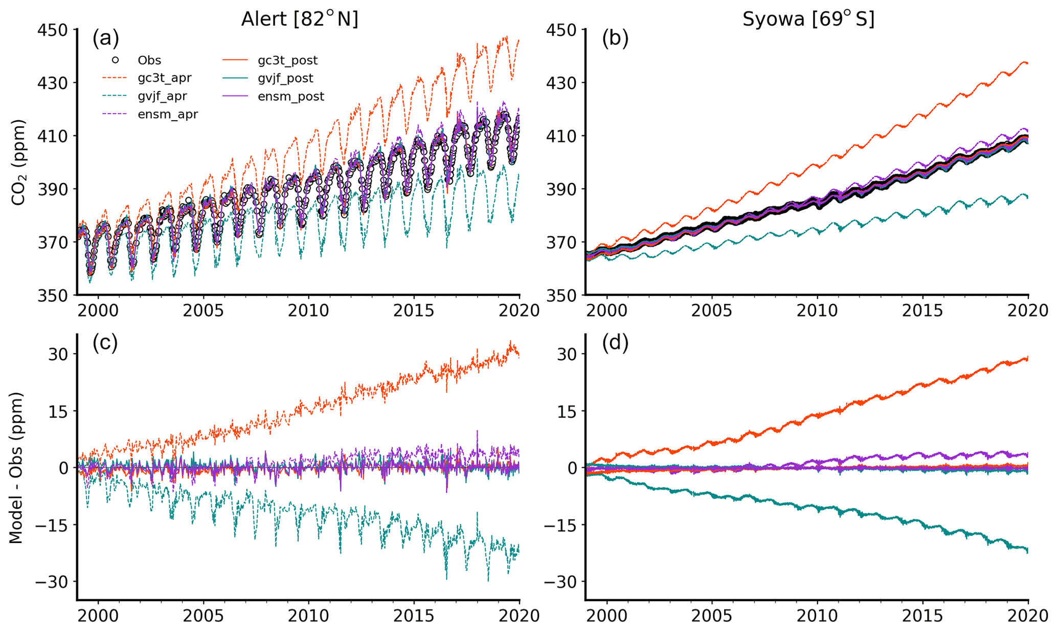
Figure 2 Time series of observed and model CO₂ time series for two a priori (apr) simulation cases (gc3t and gvjf) and posterior (post) flux simulation cases using control MDU and PFU case ux4 (a, b). Results for the mean of two a priori flux cases and ensemble mean inversion case are also shown. The model–observation differences are shown in (c) and (d). Results are shown for two sites, Alert (82^∘ N, 63^∘ W; measurements by Environment Canada) and Syowa (69^∘ S, 40^∘ E; measurements by Tohoku University/National Institute of Polar Research).

2.5 Performance of inversion using a posteriori uncertainty

The inverse model output monthly mean flux corrections and a posteriori flux uncertainty for each of the 84 regions and the full error covariance matrix of dimension 24192 × 24192 (= 84 regions × 12 month × number of inversion year). The monthly time and spatial covariances are accounted for flux uncertainty calculation when annual mean values are calculated for aggregated regions or global budgets. In the aggregation scheme, the larger regions have to follow the boundaries of 84 regions, contrary to the method proposed in Sect. 2.6 using ensemble inversions where ensemble spreads can be calculated for any region of interest.

We use flux uncertainty reduction (FUR, in %), based on the mean values without time aggregation, to identify which regions are well constrained by the data. FUR is a standard diagnostic of Bayesian estimation and is defined by

$$\mathrm{FUR}=\left(\mathrm{1}-{\displaystyle \frac{{\mathit{\sigma }}_{\mathrm{predicted}}}{{\mathit{\sigma }}_{\mathrm{prior}}}}\right)\times \mathrm{100},$$

where σ_prior and σ_predicted represent the mean prior and predicted flux uncertainties, averaged over January 2001–December 2020. High values (FUR towards 100) indicate strong data constraints, while low values (close to 0) indicate that the data are not able to move the estimates away from the prior flux. To identify which parts of the land and ocean have been constrained significantly by the inversions, PFU, predicted flux uncertainty, and FUR are plotted in Fig. 3 for the four PFU cases of the gc3t and ux4 setup. The PFU cases “gpp_v4” and ctl show observational constraint over most of the region (grey shaded areas in the right column). Reasonable constraints (larger FUR) are obtained for Northern America, Russia, Southern Ocean, Tropical Pacific, South Indian, and North Atlantic, highlighting the large long-running observational programs by US, Japanese, and European research groups. The poor constraints (low FUR) are observed over South Asia, West Asia, Northern Africa, and the Tropical Indian Ocean due to the lack of observations. It is also noted that FUR is influenced by PFU settings. For example, a smaller a priori uncertainty, i.e., gpp_v2, achieved lower FUR. As discussed later in this article, the FUR is only indicative of the observational constraint on the regional fluxes; the spread of ensemble inversions provides a measure of uncertainty of the regional CO₂ sources and sinks.

Figure 3 Prior and posterior flux uncertainties for four different PFU (four rows: ctl, “gpp_v2”, “gpp_v3”, gpp_v4) cases are shown in the left and middle column, respectively, and the flux uncertainty reduction (FUR) in the right column. The FUR is an indicator of constraint provided by atmospheric observations. High values (towards 100) in uncertainty reduction indicate strong data constraints, while low values (close to 0) indicate that the data are not able to move the estimates away from the prior flux. All cases correspond to the MDU case ux4 and gc3t inversion case. The circles show the 50 observation sites used for inverse analysis.

2.6 Flux processing and regional uncertainty estimations

The predicted fluxes from 84 regions (54 land and 30 oceans) are regridded to the $\mathrm{1}{}^{\circ }\times \mathrm{1}{}^{\circ }$ spatial resolutions based on the land and ocean basis functions. Once regridded, the fluxes were aggregated into 15 land and 11 ocean regions for further analysis (ref. Fig. 1b). First, the fluxes from each inversion are averaged for different analysis periods (monthly, annual, 5-year, decadal). Then, we averaged the individual means (n=16) to estimate the ensemble mean and standard deviations. The ensemble mean (here and, in the following, referred to as “ensm”) is the best estimate (i.e., a measure of central tendency) of land–air and sea–air exchange carbon flux. The best estimate criterion is based on the closest agreement of the global total (FFC emissions + land and ocean sinks) fluxes with the global mean growth rate (Sect. 3.2). There are different options to characterize “uncertainty” in CO₂ flux estimates, for example, the standard deviation, standard error, 95 % confidence intervals, and interquartile ranges. Here, we followed the standard deviation of the multi-inversion means as a metric of the uncertainty (i.e., variability) in the multi-inversion estimates. The regional and global land/ocean flux uncertainties estimated from the 16 ensemble members cover those that arise from priori flux distributions, PFU and MDU. The uncertainties due to data coverage and model transport errors are not assessed here.

2.7 Observations used for predicted flux validation

The predicted fluxes are validated by comparing the posterior 3-dimensional CO₂ mixing ratios fields to independent (i.e., not used in the inversions) aircraft observations. The aircraft observations used for validation include data published in obspack_co2_1_GLOBALVIEWplus_v6.1 (Schuldt et al., 2021).

2.7.1 HIPPO and ATom observations

We used the CO₂ from two sets of aircraft campaigns: the HIAPER Pole-to-Pole Observations (HIPPO) during the period 7 January 2009 to 15 September 2011 (Wofsy, 2011) and the Atmospheric Tomography Missions (ATom) during the period 29 July 2016 to 21 May 2018 (Wofsy et al., 2018) to validate the latitude–altitude gradients covering different seasons over the Pacific and Atlantic oceans. The four HIPPO campaigns (HIPPO-1 in January 2009, HIPPO-2 in October/December 2009, HIPPO-3 in March/April 2010, and HIPPO-4 in May/July 2011), performed from 82^∘ N to 67^∘ S over the Pacific (but also partly cover the North American continent) and with continuous profiling between ∼ 150 and 8500 m altitudes at approximately 2.2^∘ latitude intervals, are used for the validation. The ATom mission is built upon the HIPPO mission but with a wider horizontal extent with global coverage over the Pacific, the Atlantic, and the Arctic oceans. The comparisons performed for all the four ATom circuits occurred in July–August 2016 (ATom-1), January–February 2017 (ATom-2), September–October 2017 (ATom-3), and April–May 2018 (ATom-4). The mission consisted of 48 science flights and 548 vertical profiles over the Pacific and Atlantic basins.

2.7.2 NOAA measurements

We also used 16 NOAA regular aircraft-based vertical profiles (Figs. S7, S8) to validate the simulated vertical gradients in the troposphere (Sweeney et al., 2015). These aircraft sites are located mainly over the North American continent (Table S4). The aircraft profiles include measurements over the Southern Great Plains (SGP: 2006–2019), operated by the U.S. Department of Energy (Biraud et al., 2013). Most of the aircraft profiles range between the surface and 350 hPa. For shorter periods, flights up to 150 hPa are available for the sites Charleston, South Carolina (SCA), SGP, and Cartersville, Georgia (VAA), also covering the UTLS (upper troposphere–lower stratosphere) region.

2.7.3 CONTRAIL measurements

The CONTRAIL (Comprehensive Observation Network for Trace gases by AIrLiners) program uses automatic air sampling equipment (ASE) for flask sampling and continuous CO₂ measuring equipment (CME) for in situ CO₂ measurements (Machida et al., 2008; Matsueda et al., 2008). These instruments have been installed on several Boeing aircraft operated by Japan Airlines (JAL) with regular flights from Japan to Australia, Europe, Asia (East, South, and Southeast), Hawaii, and North America, providing large spatial data coverage across the globe, particularly in the Northern Hemisphere. The ASE performed flask samplings in the upper troposphere and lower stratosphere (altitude range of ∼ 7–12 km). The CME data are recorded at 1 s intervals during ascent/descent (∼ 100 m intervals in altitude) and at 1 min intervals during cruise (∼ 15 km intervals horizontally) as well as in-flight aircraft positions. CME is not operated within ∼ 600 m of the ground surface to avoid heavy pollution around airports. The CME has obtained thousands of CO₂ vertical profiles over many airports since 2005. The ASE and CME, along with NOAA aircraft measurements of CO_2, are used to estimate the latitudinal bias in predicted fluxes.

2.7.4 Evaluation metrics

We calculate correlation coefficients (R), mean bias (MB), and root-mean-square errors (RMSEs) to evaluate the predicted fluxes with aircraft observations. The mean bias and RMSE are defined as

$$\begin{array}{c}{\displaystyle }\mathrm{MB}=\left({\displaystyle \frac{\mathrm{1}}{n}}\sum _{i=\mathrm{1}}^n{\left(x_{{\mathrm{CO}}_{\mathrm{2}}}^{\mathrm{o}}-x_{{\mathrm{CO}}_{\mathrm{2}}}^{\mathrm{p}}\right)}_i\right)\\ {\displaystyle }\mathrm{RMSE}=\sqrt{\left({\displaystyle \frac{\mathrm{1}}{n}}\sum _{i=\mathrm{1}}^n{\left(x_{{\mathrm{CO}}_{\mathrm{2}}}^{\mathrm{o}}-x_{{\mathrm{CO}}_{\mathrm{2}}}^{\mathrm{p}}\right)}_i^{\mathrm{2}}\right)},\end{array}$$

where $x_{{\mathrm{CO}}_{\mathrm{2}}}^{\mathrm{o}}$ is observation, $x_{{\mathrm{CO}}_{\mathrm{2}}}^{\mathrm{p}}$ is predicted CO₂ mole fraction sampled at the ith aircraft location, and n is the number of aircraft observations. The MB infers the magnitude of underestimation/overestimation of CO₂ mixing ratios by the model. The RMSE includes errors (both random and systematic) in the predicted CO₂. The MB and RMSE could be due to uncertainties in predicted fluxes. Model transport is one of the sources leading to uncertainties in the predicted fluxes, but the simulations of SF₆ and the age of air confirm the low transport error in MIROC4-ACTM (Bisht et al., 2021; Patra et al., 2018). Hence, the magnitude of biases and RMSE indicates predominantly the accuracy of the predicted fluxes (the errors due to model transport and measurement network are not explored in this study).

3 Results and discussion

3.1 Global flux distributions

Figure 4 shows the spatial distributions of annual mean CO₂ fluxes. While the spatial distributions of a priori oceanic flux are similar for the JMA and TT09, the terrestrial biosphere fluxes are vastly different. The annually neutral CASA fluxes show near-zero values for most grid cells. However, strong sinks are observed over most of the densely vegetated regions of the globe for the VISIT+GFED fluxes, mainly because the VISIT simulation produces stronger sinks by the ecosystem (Fig. 4a, d). Anomalously strong sources are also seen in Fig. 4d due to the fire emissions estimated by GFED based on the satellite-derived burned area anomaly. The a posteriori results make reasonable corrections regardless of which a priori fluxes they start from, e.g., the gc3t case with net-zero annual flux or the “gvjf” case with strong sink. Consistently predicted fluxes are seen for North America, Europe, Russia, or East Asia for the PFU = ctl case (middle row). Similarities are slightly less when the PFU is scaled to the GPP of 84 regions of the inverse model (bottom row). This suggests that the greater PFU is more suitable for the inversion when the region has observational sites (Fig. 1). In the case of PFU = gpp_v2, the fluxes are not allowed to change much in the boreal regions, except for the summer months. However, the gpp_v2 inversion may be preferred over the dry region of Northern Africa, where the control PFU case produces an east (weak source)–west (weak sink) dipole. Performance of the inversions to retrieve the flux distributions over tropical America and tropical Africa is unclear. They show large dependence on the prior flux distributions, possibly due to the lack of observations within the land regions in our inversion. The main focus of this study is to better understand the total regional emissions and their trends over the past 20 years. The inversion does not revise the fine structures within each of the 84 regions of the inversion by the design of the system, where the regional basis functions assume a fixed pattern for constructing the source–receptor relationships (J matrix). The degree of freedom of our inversions is a few times smaller than the gridded inversions when spatial flux correlations of 1000–2000 km are assumed (Peylin et al., 2013).

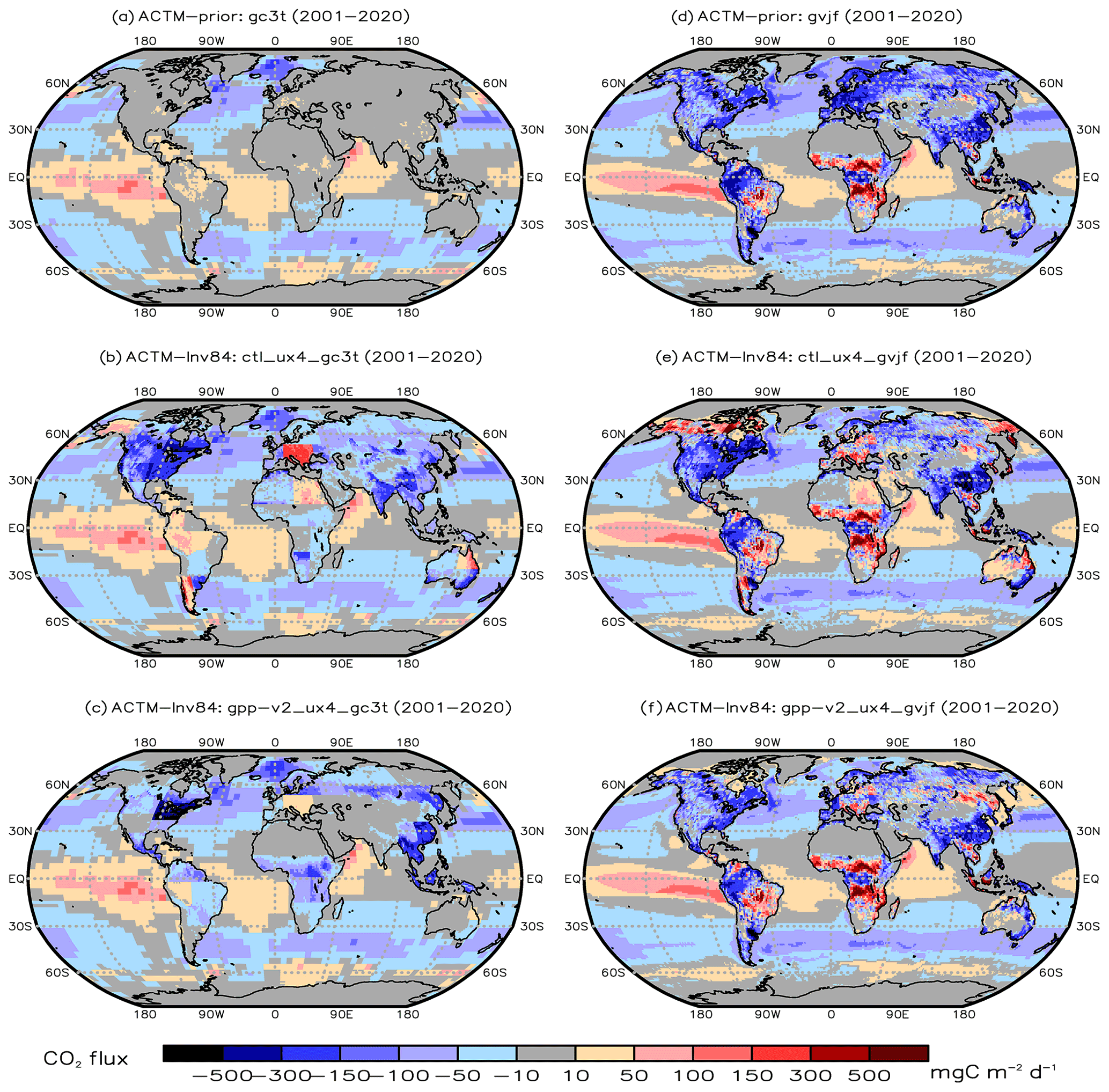
Figure 4 Spatial distributions of CO₂ prior flux for two different sets of land and ocean flux combinations (a, d). The middle (b, e) and bottom (c, f) panels show predicted CO₂ fluxes using two different prior flux uncertainty patterns (ctl, gpp_v2).

3.2 Global total fluxes

Figure 5 shows the trends and interannual variability in the global fossil fuel (FF) emissions (used as input for the inverse model), land–biosphere, ocean, and annual atmospheric CO₂ growth rate for 16 inversion ensemble members based on two combinations of land–biosphere and ocean prior fluxes (VISIT and CASA for land–atmosphere and TT09 and JMA for sea–air) and eight combinations of prior flux/data uncertainties (PFU and MDU). The uncertainty in the ensemble means the flux of 16 inversion cases is calculated using ± 1σ spread in the time-averaged fluxes for 10- or 5-year periods in this study. The uncertainties in the predicted fluxes due to different priors are 0.35 PgC yr⁻¹ for global land and 0.1 PgC yr⁻¹ for the global ocean. The uncertainty due to PFU and MDU is less than 0.15 PgC yr⁻¹ for land and ocean carbon uptake for gc3t or gvjf inversions. It indicates that prior flux patterns and trends alter the predicted global land and ocean fluxes. Ensemble mean land and ocean fluxes are in excellent agreement with the IPCC “mean” estimates, notably within the 1σ uncertainty estimated from 16 ensemble member inversions (Table 3). The ensemble spread is much lower (Table 3; MIROC4-ACTM columns) compared to the inversion-predicted flux uncertainties, which are in the range of 1.4 and 0.7 PgC yr⁻¹ for the global land and ocean, respectively, even after accounting for the monthly time and spatial covariances (vary from low values of 0.8 and 0.5 PgC yr⁻¹ for gpp_v2 cases to 1.6 and 0.9 PgC yr⁻¹ for the gpp_v4 inversions).

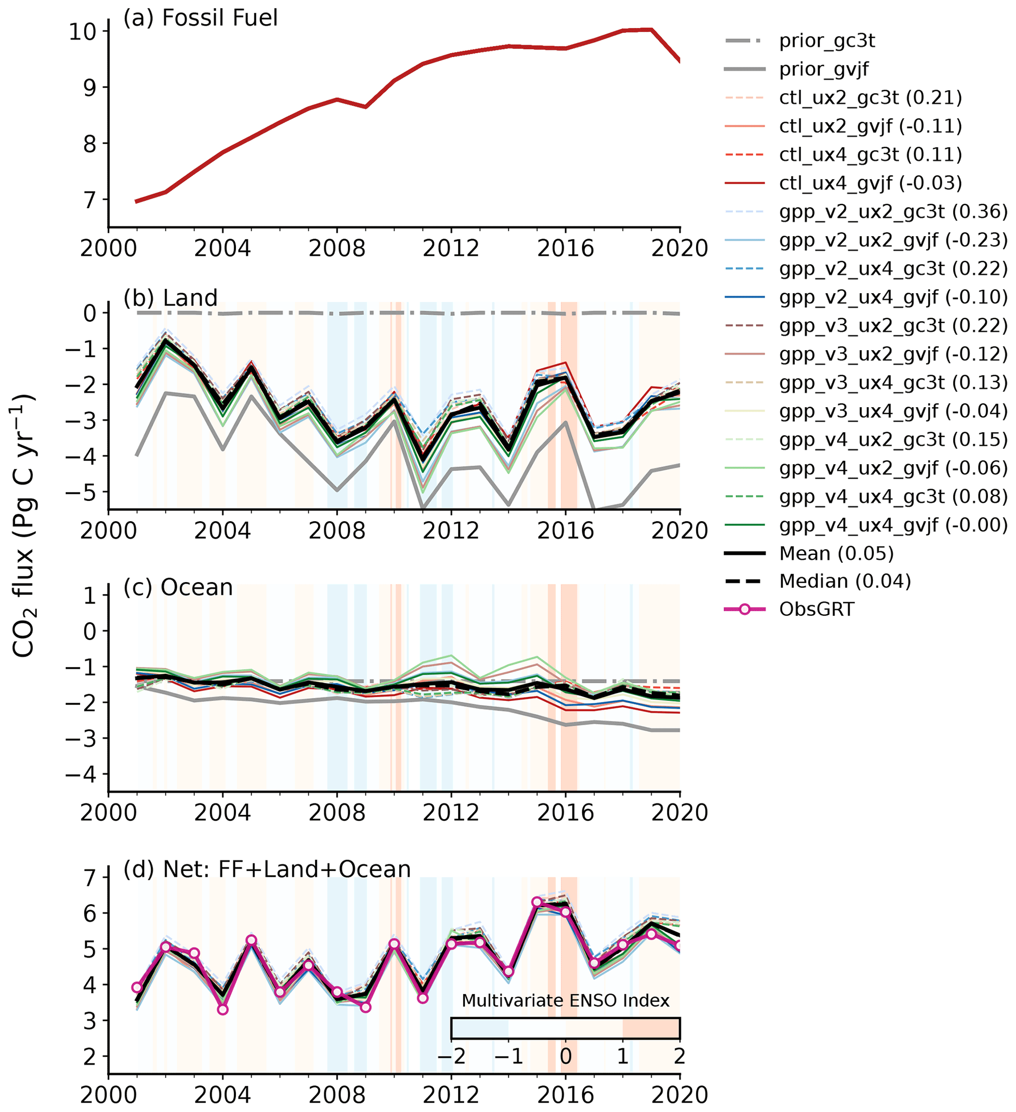
Figure 5 Global annual CO₂ emissions from fossil fuel (a) and estimated land (b) and ocean (c) carbon sink from two sets of prior and 16 sets of predicted fluxes based on different combinations of priors (gc3t and gvjf), prior flux uncertainties (PFU: ctl, gpp_v2, gpp_v3, gpp_v4) and measurement data uncertainties (MDU: ux2, ux4). Negative values show uptake by land/ocean, and positive values show sources to the atmosphere. The net flux is calculated by subtracting the total sink (land + ocean) from the fossil fuel and compared with the observed global growth rate of atmospheric CO₂ concentration from the NOAA/ESRL (magenta line in panel (d); Dlugokencky and Tans, 2020). The atmospheric CO₂ growth rate is converted using a factor of 2.13 PgC ppm⁻¹. The numbers in the brackets in the legend are the mean budget imbalance between annual means of net flux and observed CO₂ growth rate (units: PgC yr⁻¹). The background shading (positive/brown for El Niño and negative/blue for La Niña) shows the multivariate El Niño–Southern Oscillation (ENSO) index or MEI (Wolter and Timlin, 2011).

Table 3 Comparison of global total land and ocean CO₂ exchanges estimated by the inversion model with those from the IPCC 2021 (Table 5.1; Canadell et al., 2021). The inversion uncertainties due to PFU and MDU for each inversion family based on priors represent ± 1σ decadal estimates from the individual inversions. The inversion means and 1σ standard deviations are shown for two prior flux cases (8 each for gc3t and gvjf) and all 16 ensemble members (ensm). The IPCC global land and ocean CO₂ uptakes are corrected for the river export fluxes. This correction to the net ocean and land uptakes is required because the inverse model estimates fluxes across the land/ocean–atmosphere interface, while the part of the land carbon exchange is exported to the ocean via the rivers and streams.

The year-to-year variability in land and ocean carbon sink (Fig. 5b, c) shows considerable agreement across the inversion cases because of the strong constraint provided by atmospheric CO₂ measurements at the global scale due to global tracer mass conservation. The year-to-year variability in atmospheric CO₂ growth rate is linked to the variability in natural sources and sinks of carbon from land and ocean for given FFC emissions. The observed CO₂ growth rate from NOAA (Dlugokencky and Tans, 2020) is compared with the estimated CO₂ growth rate (by inversion), defined as the difference between fossil fuel emissions and total sink over land and ocean on an annual basis (Fig. 5d). The NOAA growth rate (ppm yr⁻¹) is converted to units of petagrams of carbon per year (PgC yr⁻¹) using a conversion factor of 2.13 PgC ppm⁻¹ (Raupach et al., 2011). The resulting mean carbon budget imbalance (in PgC yr⁻¹), calculated as the mean absolute difference between the inversion estimated (FFC emissions + a posteriori land and ocean sinks) and the observed CO₂ growth rates, is given in the legend (Fig. 5). The year-to-year variability in the global annual total of net CO₂ flux is robust across different inversion cases (r=0.97) and with the observed growth rates (r=0.9); however, the global totals over 2001-2020 show slight bias with that observed. Compared to the observed CO₂ growth rate, the inversion shows systematic positive (range 0.1–0.3) and negative (range 0.0–(−0.2)) imbalances for gc3t and gvjf inversions, respectively. The ensemble mean of 16 inversions (ensm) agrees well with the observed growth rate within the uncertainty of the predicted fluxes over the 20 years (Fig. 5d).

Inversions suggest that both the terrestrial land and ocean sinks increased during our analysis period 2000–2020. The ensemble means of terrestrial land CO₂ sink increased from −2.31 ± 0.21 PgC yr⁻¹ in the 2000s (2000–2009) to −2.9 ± 0.26 PgC yr⁻¹ in the 2010s (2010–2019), with significant interannual variations up to 2 PgC yr⁻¹. The interannual variability in land CO₂ flux is predominately associated with the response of the terrestrial biosphere to El Niño–Southern Oscillation (ENSO)-induced changes in the weather pattern. In 2015–2016, and to a lesser extent in 2010, El Niño conditions reduced carbon uptake by the land ecosystems in the tropics (e.g., Baker et al., 2006; Bousquet et al., 2000; Patra et al., 2005b). The average ocean sink intensified from −1.46 ± 0.10 PgC yr⁻¹ in the 2000s to −1.62 ± 0.17 PgC yr⁻¹ in the 2010s, with interannual variations of the order of a few tenths of petagram of carbon per year (PgC yr⁻¹) (Chatterjee et al., 2017; Feely et al., 1999; Patra et al., 2005a). The global ocean biogeochemistry model (GOBM) products, and those based on pCO₂ measurements, also show similar decadal variability patterns (DeVries et al., 2019; Hauck et al., 2020).

This gradual increase in the ocean CO₂ sink is caused by the increasing pCO₂ difference between the marine air and sea-surface water. The strong increase in the net sink by the terrestrial biosphere during 2001–2009 is sometimes attributed to the bias in FFC emissions from China (Saeki and Patra, 2017), and the gradual sink increase can be attributed to CO₂ fertilization or water-use efficiency as more carbon is available for assimilation by photosynthesis (Keeling et al., 2017; Kondo et al., 2018). In addition, the land CO₂ uptake efficiency in the period of this analysis could partly be controlled by a decadal shift in the frequency of natural climate variability, such as ENSO. In the 2000s, no extreme El Niño conditions were observed, resulting in suppressed fire emissions and lowered drought occurrences, while the opposite conditions prevailed in the 2010s (intense El Niño in 2010, 2015–2016, and 2019–2020), which is likely to reduce net uptake by the land ecosystems (Patra et al., 2005b). Fire emissions with an estimated peak-to-trough change of about 0.5 PgC yr⁻¹ (Table 1) alone cannot explain the large changes in land sinks of the order of 2–3 PgC yr⁻¹.

3.3 Subcontinental-scale land and ocean fluxes

Here, we present interannual variability in a priori and predicted carbon fluxes over 15 lands (Fig. 6) and 11 ocean regions (Fig. 7). The uncertainty in the predicted carbon fluxes is estimated as 1σ spread among the 16 inversion cases. Significant differences are seen between a priori (VISIT) fluxes over Russia (−0.76 PgC yr⁻¹), East Asia (−0.55 PgC yr⁻¹), and Europe (−0.54 PgC yr⁻¹) and ranges of inversion estimations −0.33 to −0.37, −0.42 to −0.57, and 0.08 to −0.09 PgC yr⁻¹, respectively. In general, the inversions suggest substantial uptakes over Temperate North America (−0.59 ± 0.14 PgC yr⁻¹), followed by East Asia (−0.49 ± 0.09 PgC yr⁻¹), Boreal North America (−0.38 ± 0.1 PgC yr⁻¹), and Russia (−0.35 ± 0.05 PgC yr⁻¹) for the study period.

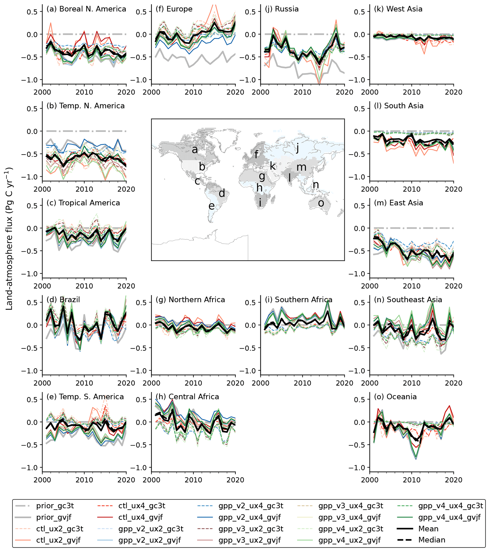
Figure 6 Interannual variation of terrestrial land CO₂ fluxes derived from 16 sets of inversion. The variations are shown for 15 aggregated regions shown in the map. The negative values are counted as CO₂ removals from the atmosphere, while CO₂ emissions are counted positively.

The large spread in the predicted fluxes over Temperate North America, Temperate South America, and Europe indicate that the estimated flux is more sensitive to the selection of PFU and MDU when there are measurement sites within the region or in the neighborhood. The carbon fluxes over tropical (Tropical America, Brazil, South Asia, and Southeast Asia) and extratropical (Temperate South America, Central Africa, Southern Africa, and Oceania) land regions are found relatively less certainly; the ensemble of inversions splits into weak source or sink groups based on the land priors. For example, inversions using the VISIT flux show a net source signal over all the three African regions, while those using the CASA flux exhibit a net sink. Similarly, all inversion cases based on the CASA prior flux show almost no carbon sink for South Asia, while VISIT-based inversion cases show a net sink of −0.18 ± 0.11 PgC yr⁻¹. The VISIT prior flux consists of strong sinks over all three South America regions. For all the regions, the inversions moderated the sinks, thus producing fluxes closer to the inversions using the CASA prior flux even though the regions have no measurement sites (Fig. 6; Table S2). These regions of Africa, South America, and South Asia are weakly constrained in the inversions due to the limited observations representing these regions. However, for most of these regions lacking in observations, the VISIT- and CASA-based inversions are moving toward a common flux value; i.e., the range of the two prior fluxes is usually much greater than the 16-inversion ensemble spread.

The predicted land carbon sink over East Asia tends to increase, which is tied to a rapid increase in FFC emissions for 2001–2009. The rapid increase in CO₂ emissions from FFC could impose an artificial trend in the terrestrial land flux estimate for the East Asia region (Saeki and Patra, 2017). Because the atmospheric data constrain the total net surface flux regionally when fluxes are constrained by observations, a biased high increase in fossil fuel emissions is required to be compensated by a biased high increase in the natural land uptake by inversion. If there are absolutely no constraints by observations, the compensation will occur in the regions where the prevailing winds transport the biased FFC signals. The South Asian uptake remains almost constant for the study period. For West Asia, both sets of inversion show the land CO₂ flux fluctuates around zero with slight interannual variation, indicating a stable trend of land flux changes and a small contribution to uptake of all the tropical regions. The annual trend in Southeast Asian carbon fluxes is overwhelmed by large interannual variability, driven mainly by ENSO-induced fire emission variability (Patra et al., 2005b; van der Werf et al., 2017). Over the African continent, Central Africa shows the highest interannual variability, mainly due to biomass burning emissions under the influence of ENSO. The CO₂ flux anomalies in the case of gvjf inversions support the fire emission anomalies taken from GFEDv4.1s as included in the prior flux, and what is more impressive for us is the ability of the gc3t inversions to produce a similar phase and magnitude of the flux variabilities, starting from a prior flux that has no interannual variability (even for these relatively unconstrained regions).

Figure 7 shows good agreement among the predicted fluxes for the 11 ocean regions and the decadal flux variability, which are derived from the TT09 prior flux with no interannual variability and the JMA flux, including interannual variability. The inversion results show substantial changes in the estimated interannual variability caused by the assumed PFU and MDU. The Northern Ocean shows a significant spread from the mean (−0.13 ± 0.14 PgC yr⁻¹) for higher MDU, particularly for 2011–2015 (−0.01 ± 0.06 PgC yr⁻¹) in the gvjf inversions. In the opposite phase a similar spread is also found for the neighboring Boreal North America, Europe, and Russia land fluxes. Because the flux variabilities over land regions are larger than ocean regions (by about a factor of 2), the Northern Ocean fluxes can be perturbed by relatively unnoticeable anomalies in the neighboring land fluxes. These features appear likely because of the incomplete measurement constraint in the inversions that permits “dipoles” of flux errors to occur between the neighboring regions (compensating for errors of opposite sign due to the inability of the measurements to completely correct the source or sink in the right place). It is indicative that an analysis of fluxes for one region may be challenging to interpret when isolated from the rest of the world in an inversion of long-lived species because of the large-scale mixing by transport.

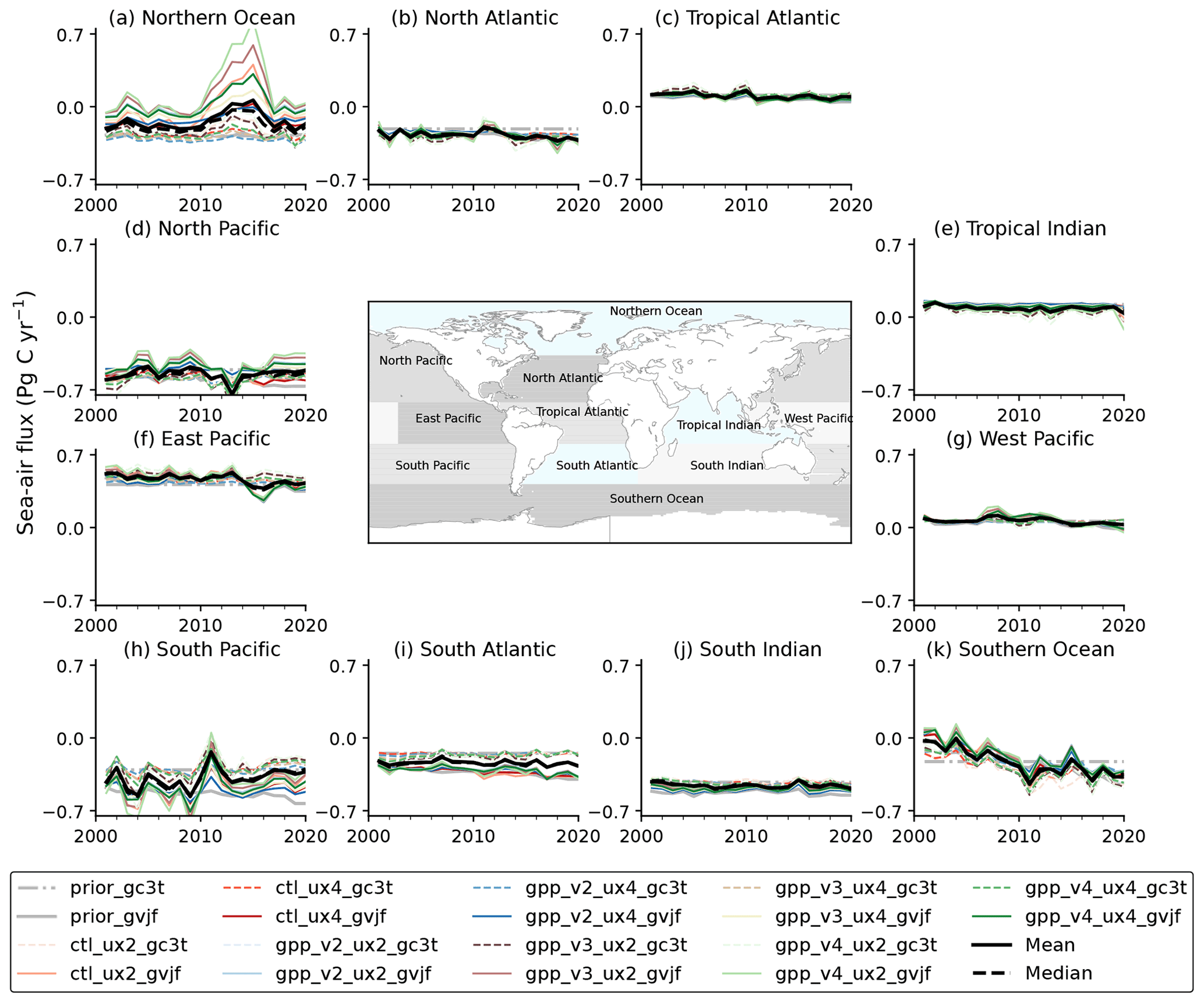
Figure 7 Interannual variation of sea–air CO₂ fluxes derived from 16 sets of inversion. The variations are shown for 11 aggregated regions shown in the map. The negative values are counted as CO₂ removals from the atmosphere, while CO₂ emissions are counted positively.

A significant difference in the priors over the South Atlantic is observed; the JMA fluxes suggest a 2-fold higher CO₂ uptake (0.33 PgC yr⁻¹) than in the TT09 (Table S2). The inversion results largely follow their priors over this region, which is observationally unconstrained by sites within the region. Both the prior and predicted fluxes show that the East Pacific is a significant source of CO₂ to the atmosphere, caused by the upwelling of deep ocean water (that brings CO₂-rich water from the ocean interior to the surface) off the west coast of the South American continent. A small net outgassing signal occurred over the Tropical Indian and Tropical Atlantic oceans. Because of a tighter constraint due to the relatively extensive coverage of observation sites, all 16 predicted fluxes converged on consistent Southern Ocean decadal trends and interannual variability, even though we have not accounted for interannual variability or trends in the TT09 prior flux. The Southern Ocean CO₂ sink intensity shows considerable variability from interannual to decadal timescales, and sink stabilization after 2010 may have been caused by a regional shift in sea level pressure and surface winds (Keppler and Landschützer, 2019).

3.4 Interannual variations in regional CO₂ fluxes

To examine the regional pattern of anomalies in the land and ocean CO₂ sink, following Patra et al. (2005a, b), we calculated the monthly anomalies by subtracting a long-term mean seasonal cycle from the monthly emissions from 2001–2020 (Fig. 8). Thus, the time series contains the interannual variability (IAV) and long-term trends for the analysis period. The anomalies from both inversion cases are consistent over most regions; however, the magnitude differs. Despite the absence of IAV in the “gc3t” prior fluxes, the consistent interannual variability suggests that inversion is robust in constraining the IAV in carbon fluxes. The correlations between gc3t and gvjf inversions over land are greater than 0.7, which are statistically significant at p<0.0001. The correlations were less than 0.3 between the gc3t inversion and the gvjf prior fluxes, which can be inferred as only some of the interannual variabilities were present in the gvjf prior fluxes, and the interannual flux variability for gvjf inversions is significantly different from the gvjf prior fluxes. These results imply that the VISIT land ecosystem fluxes and GFEDv4.1s fire emissions inadequately represent CO₂ flux signals that are observed at the 50 measurement sites in our inversion. Large-scale cyclic patterns of climate anomalies such as ENSO account for a large part of CO₂ flux variabilities on interannual to sub-decadal timescales. Climate anomalies are associated with changes in temperature distributions and large-scale circulations of the ocean water and the atmosphere.

Figure 8 The 3-monthly running averages of CO₂ flux anomalies as estimated by the inversions for land and ocean regions from atmospheric CO₂ data, with varying prior flux uncertainty and different a priori emissions. The flux anomaly is calculated by subtracting an average seasonal cycle from 1999–2020 from the monthly-mean CO₂ fluxes. The cases shown in the panels are obtained by the gvjf prior fluxes (thick grey line), an average of all gc3t inversion cases, and gvjf inversion cases. The ±1σ around the mean of both inversion cases is shown as shading. The ENSO index is plotted in the background for the corresponding period. The correlations between fluxes (predicted and prior) and multivariate ENSO index are shown in Table S3.

The CO₂ flux anomalies in the tropical regions are strongly correlated with the ENSO index, while temperate and boreal regions are weakly correlated, as expected from the areas of ENSO influences (Table S3). In the northern high latitude regions of Europe, America, and Asia, a negligible correlation was found between CO₂ flux anomalies and the ENSO index. It is because, over these regions, the North Atlantic Oscillation (NAO)/Arctic Oscillation (AO) or Pacific Decadal Oscillation (PDO) is the dominant climate factor for the CO₂ flux anomaly, likely through the temperature variation (Patra et al., 2005). The warmer weather in these regions may lead to a negative CO₂ flux anomaly (Russia) since that condition stretches the growing season length (Dye and Tucker, 2003). The correlation coefficient between CO₂ flux anomalies for different aggregated land and ocean regions is given in Table S3.

In 2015, a strong El Niño induced severe drought and biomass burning in equatorial Asia. It was one of the most significant El Niño events after the well-known major El Niño in 1997/1998 (L'Heureux et al., 2017; Santoso et al., 2017). Patra et al. (2005b) estimated that a massive amount of carbon (∼ 5.5 PgC yr⁻¹) was released into the atmosphere in 1997/1998, largely contributed from tropical regions in Asia, South America, and Africa. Figure 8 shows that during the extreme El Niño period in 2015–2016, a large amount of carbon was also released from Tropical America and Southeast Asia, followed by Central Africa and Brazil. However, the timing and strength of the peaks are different. The fire emission peak (for gvjf case) appeared in August 2015 over Southeast Asia (1.34 PgC yr⁻¹) and in January 2016 over Tropical America (1.12 PgC yr⁻¹). The gc3t inversion suggests a peak in October 2015 for Southeast Asia (0.42 PgC yr⁻¹) and in January 2016 for Tropical America (0.82 PgC yr⁻¹). Niwa et al. (2021) showed that regular sampling of aircraft CO₂ measurement under the CONTRAIL project has enormous potential for capturing the footprint of biomass burning. By advanced inverse analysis, they estimated equatorial Southeast Asia emission at 0.27 PgC yr⁻¹ during September–October 2015 (note that northern Southeast Asia is not included).

Over the Oceania regions, the gvjf inversion shows large interannual variability. The inversion suggests emission peaks in 2019–2020 over Oceania, consistent with the substantial CO₂ released from the fire in the atmosphere during the 2019–2020 summer season over Australia (van der Velde et al., 2021). They concluded that the CO₂ emission from these fires was more than thrice the estimate derived from the long-term mean of CO₂ uptake over this region and broadly consistent with estimates based on the GFED fire emissions. van der Velde et al. (2021) estimated a CO₂ flux anomaly in the range of 0.14–0.24 PgC from November 2019 to January 2020, which is lower than our estimation of 0.7 PgC.

The gc3t CO₂ flux variabilities over East Pacific, West Pacific, and South Pacific show negligible correlations with ENSO, while both JMA-based prior and posterior fluxes show high correlation (Table S3). Over the North Pacific, both inversion ensembles show an insignificant correlation with ENSO. The oceanographic observations indicate that sea surface temperature and pCO₂ in the equatorial warm pool areas (5^∘ N–5^∘ S, west of the dateline) are not sensitive to El Niño conditions (Takahashi et al., 2003), but a strong correlation is found for the West Pacific region in the case of the JMA ocean prior flux that is driven by pCO₂ measurements and sea surface temperature. Due to the lack of observational coverage, the gc3t inversions did not produce an expected (negative) correlation for CO₂ fluxes and ENSO index for the East and West Pacific regions. Patra et al. (2005a) showed that the global ocean flux variability is significantly underestimated or even produced the opposite phase for strong El Niño of 1997/1998 if the Pacific Ocean cruise data are not used in inversions. CO₂ flux anomalies are estimated to be positive for South Pacific and negative for East Pacific during the 2015–2016 El Niño event. On the contrary, observations show that the sea-to-air CO₂ flux is suppressed during the intense El Niño event by warm low-CO₂ surface waters from the west. The atmospheric observations are limited over these regions. Thus, we consider that the anomalies during the intense El Niño period 2015–2016 are likely to be an artifact because of the lack of observational constraints. The interannual variability over the tropical Atlantic, tropical Indian, and south Indian is low. Though the IAV is low, we find a significant correlation for the tropical Atlantic for both predicted fluxes, in contrast to a negligible correlation between the prior flux and ENSO.

3.5 Mean seasonal cycles of regional CO₂ fluxes

The net CO₂ uptake in the moist and warm growing season is partially compensated by net CO₂ release in the dry and cold non-growing season. However, the magnitude of seasonal compensations differed significantly between regions. The compensation drives the net regional strength of CO₂ uptake. For example, the maximum uptake in the growing season is shown by Russia (∼ 10 PgC yr⁻¹), followed by Boreal North America (∼ 5 PgC yr⁻¹) and Temperate North America (4 PgC yr⁻¹) (Fig. 9). However, the strength of net sink is almost twice over Temperate North America (−0.59 ± 0.14 PgC yr⁻¹) than in Russia and Boreal North America because the release of CO₂ in the non-growing season over Russia and Boreal North America is greater than Temperate North America. Thus, the seasonal cycles in global and regional emissions are essential for understanding the drivers of CO₂ changes in the atmosphere.

The seasonal cycle amplitude for the CASA prior flux for the land total is 33.6 PgC yr⁻¹, and that for VISIT is weaker at 23.8 PgC yr⁻¹, and the peak of the growing season (when the net flux is most negative) occurred in July for CASA that is 1 month after VISIT (Fig. 9, top-left panel). The seasonal phase of gc3t-predicted fluxes are in close agreement with the CASA prior, but inversions diverge for the net CO₂ uptake in the growing season and release in the dormant season. Our inverse analysis indicates a more considerable CO₂ uptake rate (−26.2 ± 2.1 PgC yr⁻¹; June–July) and net CO₂ release rate (4.1 ± 2.0 PgC yr⁻¹; January–April) than CASA-based terrestrial land flux. Contrary to the CASA prior, inversions using the VISIT prior flux increase sinks significantly, by up to about 10 PgC yr⁻¹, in June–July compared to the a priori flux. Inversion fluxes using CASA and VISIT show high consistency for the total land CO₂ flux seasonality. Overall, the averaged gc3t and gvjf show good agreement (r=0.98) after inversion as compared to a priori (r=0.8). Inversions do not achieve similar consistency for the total global ocean fluxes for both TT09 and JMA a priori fluxes (third row from bottom, left column); the correlations reduced from 0.95 to 0.58 after the inversion.

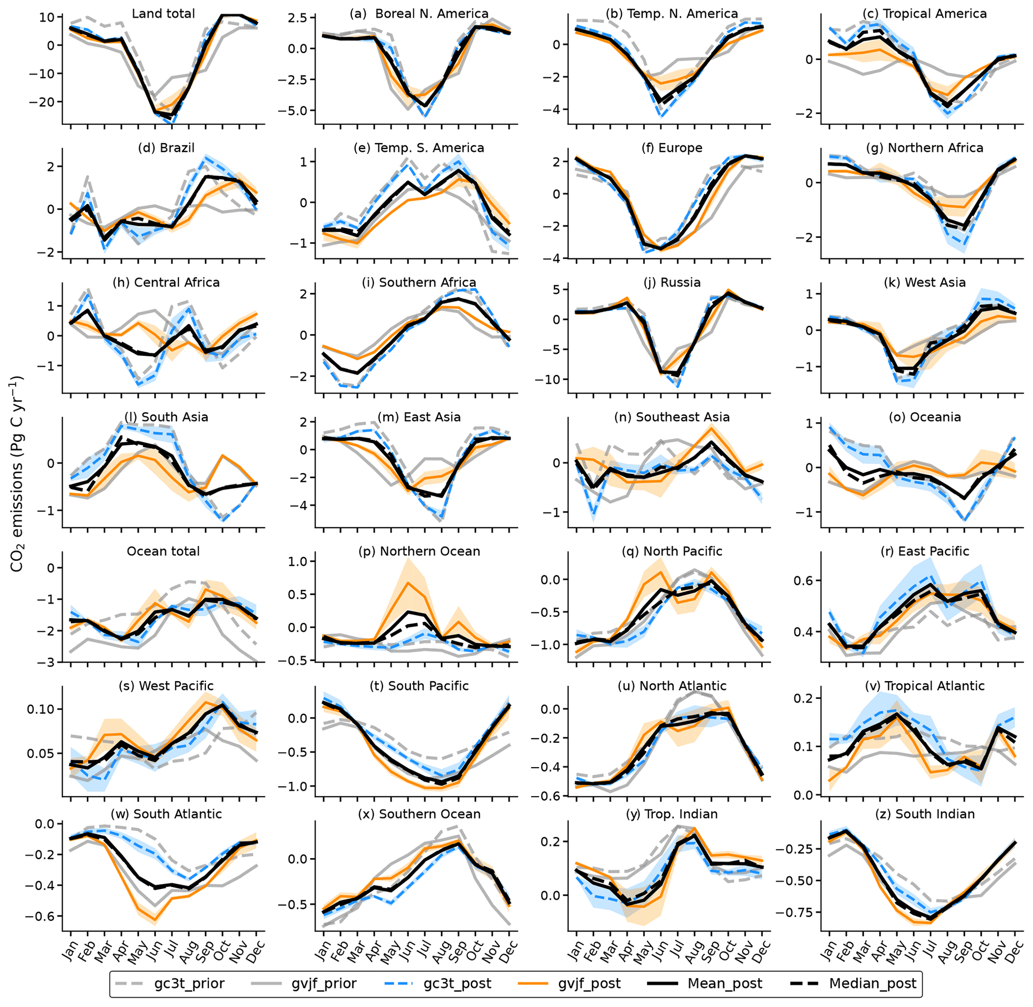
Figure 9 Seasonal variations in monthly-mean CO₂ fluxes at regional scales over 15 lands (upper four rows) and 11 oceans (lower three rows) regions, along with global land and ocean totals. We prepare the average (2001–2020) separately for inversion ensemble cases based on gc3t (broken line) and gvjf (solid line) prior. The shade around means shows ±1σ SDs for the respective inversion cases. The individual inversion cases are plotted in the Supplement (Fig. S2). Note that all panels use different y scales.

Northern land fluxes drive the global land seasonality, with a close agreement regarding the magnitude and phasing of the growing season and dormant season fluxes. Seasonality for the tropical land (South Asia, Tropical America, Central Africa, Southeast Asia) is smaller than the northern land regions (Boreal North America, Temperate North America, Russia), with the inversion suggesting maximum uptake around June–July over northern land and July–September over tropical land. The a priori and predicted fluxes are more consistent for the extratropical land regions than their tropical counterparts. This is because the temperate biosphere is better simulated by the ecosystem models, such as VISIT or CASA, by taking into account the temperature and light effects, while the tropical ecosystems are more often limited by water availability or suffer from extreme heat, e.g., the monsoon driven South Asia (Patra et al., 2013). Posterior fluxes for the tropical regions also do not converge well, mainly because of the general sparseness of CO₂ data (Patra et al., 2013).

Over Tropical America, CASA shows maximum carbon uptake (flux = −2.0 PgC yr⁻¹) in August and an extended-release period in the dormant season from January to April (flux = 1.1 PgC yr⁻¹), while VISIT shows a relatively small seasonal variation. However, the inversions derive a consistent seasonal phase and amplitude, although the region does not include any measurement site. Thus, the adjoining neighborhoods' observations are helping us to capture the signal from this region, which is probably enabled by a good transport simulation by MIROC4-ACTM. A similar improved consistency in predicted seasonal cycle phase and amplitude, relative to the a priori, is also obtained for many other regions (Fig. 9a, b, c, f, g, k, n). Nevertheless, the a priori models play significant roles in estimations of CO₂ flux seasonality for South Asia (peak uptake flux −0.43 PgC yr⁻¹ in August–September for VISIT and −1 PgC yr⁻¹ for CASA in October–November), and East Asia (CASA peak uptake in August, VISIT peak uptake in April).

The global ocean prior fluxes show the weak uptake of CO₂ during July–September (average uptake flux of −0.53 ± 0.09 PgC yr⁻¹ for TT09 and −1.12 ± 0.14 PgC yr⁻¹ for JMA). From September onwards, a sharp increase in uptake occurs, with a maximum uptake of 2.43 PgC yr⁻¹ for TT09 and 2.91 PgC yr⁻¹ for JMA fluxes in December (Fig. 9, left, third row from bottom). Over the Northern Ocean, the gvjf inversion cases tend to show a large CO₂ release as the MDU increases during May–October. We believe the broader uptake seasons for Boreal North America, Europe, and Russia, leading to stronger early summer land uptake in the case of VISIT a priori, caused positive CO₂ flux seasonality for the Northern Ocean. Even for the gc3t inversion case, we find the peak in the seasonal cycle in the summer season, when the oceanic biosphere activity is at its peak and pCO₂ in water is lower in summer than in the winter (Goto et al., 2017; Yasunaka et al., 2018). It is not easy to put forward a hypothesis for the weaker sink in summer than in winter of the Northern Ocean, while we can speculate that the atmospheric CO₂ decrease in polar air due to the strongest flux seasonal cycle on boreal land (Fig. 9a, f, j) exceeds the decrease that occurs over the surface seawater and reduced solubility of CO₂ in warmer water. Indeed, Yasunaka et al. (2018) have shown that the Greenland–Norwegian seas and the Barents Sea indeed act as a milder sink of CO₂ (flux = −4 to −5 mmol m⁻² d⁻¹) during June–August compared to the October–March (flux = −10 to −15 mmol m⁻² d⁻¹), and the Chukchi Sea and Arctic Ocean show the strongest uptake in October. Thus, as a whole, the Northern Ocean of our study could act as the weakest sink in the summer months. Further studies are needed to identify the role of ice-covered areas (close to zero CO₂ flux) in the seasonal cycle. Note here that the oceanic basis functions in the polar ocean regions use a climatological sea-ice cover map, and fluxes are not revised over the sea-ice-covered areas.

Overall, all the land regions, except South Asia, Southeast Asia, Central Africa, and Oceania, show excellent agreement between averaged gc3t and gvjf cases after inversion (r = 0.63–0.97), as compared to the prior flux (r = −0.48–0.90). A good agreement over the Northern Ocean, West Pacific, and Tropical Atlantic Ocean seasonal cycle is observed after the inversion (Table S3).

3.6 Regional CO₂ fluxes and flux uncertainties

Different regions across the globe emit different amounts of CO₂ from FFC emissions, which is one of the main discussion points in the emission reduction policymaking, e.g., under the Kyoto Protocol (1997) and Paris Agreement (2015), for limiting global warming below a certain level. The recent IPCC AR6 of Working Group I suggested that the global total CO₂ emissions from FFC have to be removed gradually on a net annual basis by 2050 to sustainably limit global warming below 1.5^∘C (Canadell et al., 2021). Because the elimination of FFC usage is challenging to envisage in the coming 3 decades, pathways for reducing FFC emissions are being explored. Carbon capture and storage and other technological management are considered alongside nature-based solutions. The land and ocean have been helping to remove more than 50 % of the FFC emissions in the past decades. The ongoing natural sinks of CO₂ and their maintenance/enhancement constitute the major theme of the nature-based solutions. Thus, it is imperative to understand global and regional carbon fluxes for developing national and international policy to reduce net CO₂ emissions.

Figures 10, S3, and S4 show regional CO₂ fluxes and flux uncertainties from the 16-member ensemble inversions for 15 land and 11 ocean regions and global land and ocean at 5-year intervals for the past 2 decades. The global flux uncertainties are found to be smaller than the regional flux uncertainties because the former are constrained strongly by the atmospheric CO₂ growth rate for given FFC emissions. Flux estimates for all the land regions remain quite uncertain, as seen from the 5 to 95 percentile range of the 16-inversion ensemble (whiskers) at about 0.3 PgC yr⁻¹ for the land regions and typically less than 0.2 PgC yr⁻¹ for the ocean regions. The fluxes at the 25 to 75 percentiles range show slightly reduced uncertainties – a large reduction is not seen compared to the 5 to 95 percentile range because the two a priori models often formed two different sets of CO₂ flux values (ref. Figs. 6 and 7). However, it has to be noted that each of the 15 land analysis regions has predicted flux uncertainties in the range of 2.1 (Boreal North America) to 3.8 (West Asia) PgC yr⁻¹ for the control gc3t case, as the reduction from prior flux uncertainties was small by inversion for most of the region (Fig. 3). Thus, by employing the 16-inversion ensemble approach, we could obtain flux uncertainties that are smaller and often less than the regional fluxes themselves. The mean/median fluxes are consistent for the ensemble inversions and represent the true state of CO₂ flux estimation for the MIROC-ACTM and 50 sites used in the inversion.

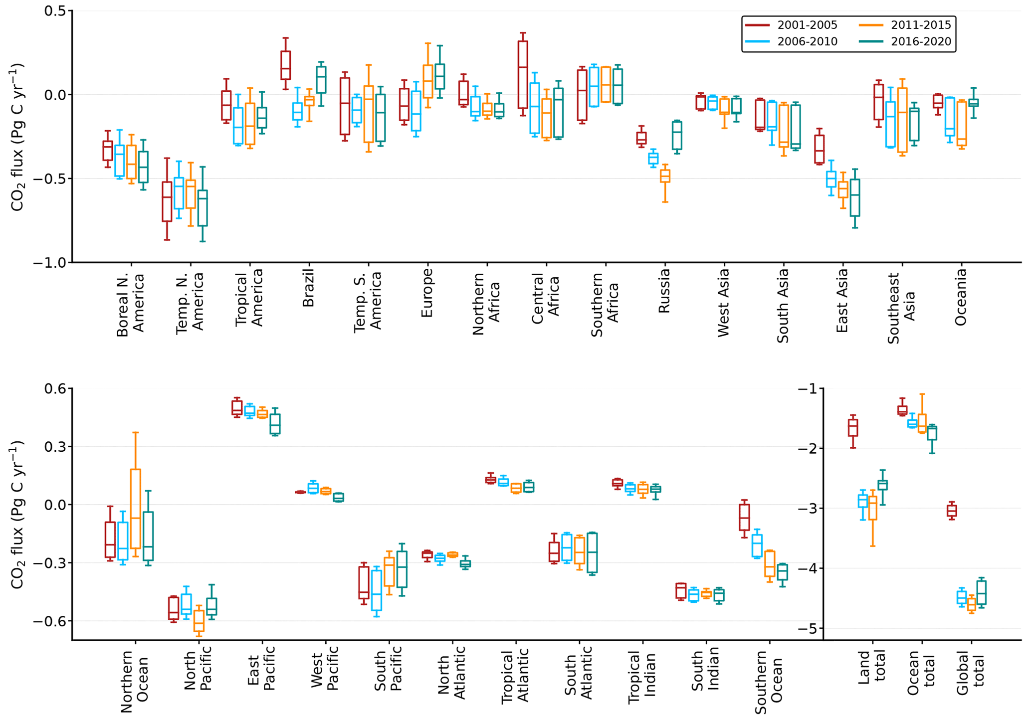
Figure 10 CO₂ fluxes for land and ocean sink using 16 sets of inversion cases. Box plots represent inversions for different time periods. Based on different prior fluxes, PFU, and MDU, the different inversion cases are first averaged for the selected time period. The box shows 25 and 75 percentiles spread, and the vertical line shows 5 and 95 percentiles from the mean CO₂ flux of 16 ensemble inversion cases. Horizontal lines inside box plots denote the median CO₂ flux of 16 inversion ensembles. Mean and spread for the whole study period (2001–2020) are given in Table S2.

Global land sink increased by ∼ 63 % from 2001–2005 to 2016–2020, with an uncertainty range of ∼ 6 %–12 %. The highest increase (about 73 %) in the land sink is observed from 2001–2005 to 2011–2015, while a decrease (∼ 11 %) is observed from 2011–2015 to 2016–2020. The northern extratropical land accounted for ∼ 80 % of the global land sink, followed by tropics (∼ 13 %) and southern extratropical land (∼ 7 %) (Fig. S3). The ocean carbon sink shows a gradual increase (by ∼ 30 %) from 2001–2005 to 2016–2020. The southern extratropical land represents about 85 % of global ocean sink for 2001–2020, followed by the northern extratropical land (∼ 60 %). The tropical ocean regions act as a net source of carbon emissions, representing 45 % of the global ocean carbon sink (Fig. S4). One of the most intriguing features is that the 5-year mean fluxes for the ocean have increased gradually, as expected from the increase in pCO₂ partial pressure difference due to increased loading of FFC emissions, but the land flux increases only during 2001–2005 and 2006–2010. This step increase in flux could be related to the biased FFC emissions from China, affecting the natural/managed land flux estimation by inversion (Saeki and Patra, 2017).

Amazonia in Brazil hosts the Earth's largest tropical forest and hence is an important region of carbon sink. Our study shows a slight decrease in carbon sink over this region from 2011–2020. A recent study based on aircraft measurements (Gatti et al., 2021) also suggests a decline in carbon sink from 2010–2018 over Amazonia due to factors such as deforestation and climate change. A very high correlation is also seen for the interannual and decadal variations in CO₂ fluxes (Figs. 6d, 10) and the Brazilian Amazon deforestation rate, which showed a strong and systematic decline from the period 2002–2004 to 2012–2014 and a steady increase afterward (Silva Junior et al., 2021).

Our results show that Africa is a small sink of carbon on an annual scale, agreeing with the RECCAP-1 estimation for 2000–2009 (Table 4). At the subregional level, northern Africa shows a small sink, while Central and Southern Africa show a minor source for the same period. Central Africa turned from a small source in 2000–2009 to a sink in 2010–2019, while the carbon flux behaviors remained persistent for the Northern and Southern Africa regions. Though Central Africa is the main carbon sink region over the African continent because of its evergreen tropical forest, the prolonged dry season due to weak El Niño during 2001–2005 could have turned it into a net source for the 2000s. The average annual mean fluxes over East Asia for the 2000s are remarkably consistent with the RECCAP estimates (Table 4), based on the average estimate from inventory, bottom-up, and inversion fluxes (Piao et al., 2012). We have observed less sink for Russia than RECCAP best estimate (Dolman et al., 2012). Other regional fluxes also agree well with RECCAP estimates, although the period and regional boundaries of the RECCAP assessment do not match precisely (Table 4).

Table 4 Mean ± 1σ standard deviation of annual net land–atmospheric exchange of CO₂ (in PgC yr⁻¹) from predicted fluxes for 15 land regions by decade. The predicted fluxes are shown for the best estimates, obtained from the ensemble mean of all 16 inversion cases based on different priors (gc3t and gvjf) and uncertainties (MDU and PFU). The ± 1σ in the decadal mean fluxes denotes the range of uncertainty. The estimations for the 2000s are compared with the REgional Carbon Cycle Assessment and Processes phase 1 (RECCAP-1).

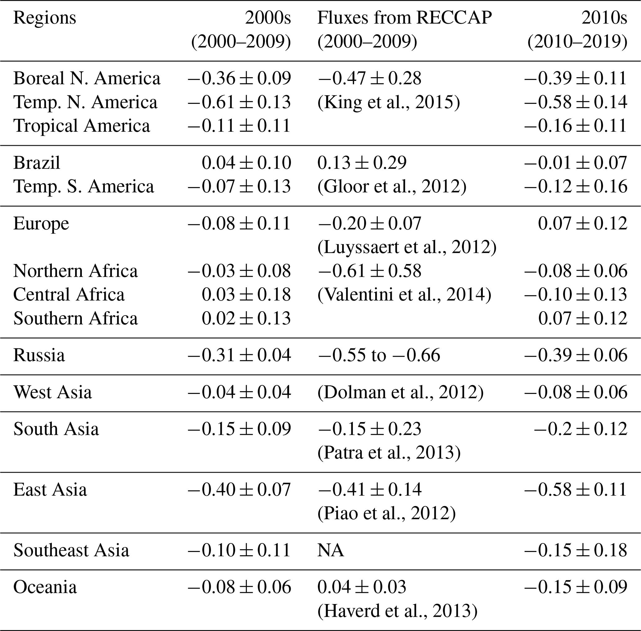
NA: not available.

Our analysis suggests that the most prominent land carbon sink in the Northern Hemisphere is located in Temperate North America (−0.59 ± 0.14 PgC yr⁻¹), followed by East Asia (−0.49 ± 0.09 PgC yr⁻¹), Boreal North America (−0.38 ± 0.10 PgC yr⁻¹), and Russia (−0.35 ± 0.05 PgC yr⁻¹) for 2001–2020, and they account for 70 % of the total global CO₂ uptake by land biosphere. Overall, our results suggest about 40 % of Temperate North America's (1.49 PgC yr⁻¹), 17 %–19 % of East Asia's (2.74 PgC yr⁻¹), 200 % of Boreal North America's (0.19 PgC yr⁻¹), and 80 % of Russia's (0.44 PgC yr⁻¹) CO₂ emissions from FFC are offset by carbon accumulation in their terrestrial ecosystems for 2001–2020. Overall, no area shows net carbon source from the land biosphere for recent decades (2010–2019). Further, the inversion suggests substantial oceanic CO₂ uptake is in the North Pacific, with a mean flux of −0.55 ± 0.05 PgC yr⁻¹. A considerable rate of CO₂ uptake is also observed in the Southern Ocean region; the CO₂ flux increased from −0.12 ± 0.07 PgC yr⁻¹ in 2001–2009 to −0.33 ± 0.06 PgC yr⁻¹ in 2010–2019. The Southern Ocean CO₂ flux for 2010–2019 agrees well with a recent assessment of −0.53 ± 0.23 PgC yr⁻¹ (net uptake) in the region south of 45^∘ S during 2009–2018 (Long et al., 2021).

3.7 Validation of CO₂ fluxes using aircraft data

We evaluate the quality of inversion flux estimates by comparing CO₂ simulations with independent observations (observations that are not used in the inversions due to a lack of long measurement time series record). The CO₂ simulations are derived from three sets of prescribed fluxes: gc3t (case: ctl_ux4_gc3t in Table 2), gvjf (case: ctl_ux4_gvjf), and ensm (average of all 16 inversions). The observations in the lower troposphere (from surface to ∼ 2 km) are more sensitive to regional fluxes. Hence, we compare the simulated CO₂ with that measured by HIPPO and ATom airborne campaigns in the lower troposphere. Figure 11 shows comparisons over the transects from high northern (∼ 80^∘ N) to high southern latitudes (∼ 70^∘ S) at the location and time of HIPPO and ATom airborne campaigns, spanning all four seasons. HIPPO shows the lower CO₂ over 30–80^∘ N than 0–30^∘ N for May–July due to the large uptake in high northern latitudes; however, the values are slightly higher than Southern Hemisphere (Figs. 11, S5). ATom shows a lower concentration over 30–80^∘N than the rest of the latitudes during July–August (Figs. 11, S6). All the model cases capture the meridional gradient, slope, and other features well at RMSEs less than 1.5 ppm, mean bias in the range −0.5–(−0.3) ppm, and correlation greater than 0.8.

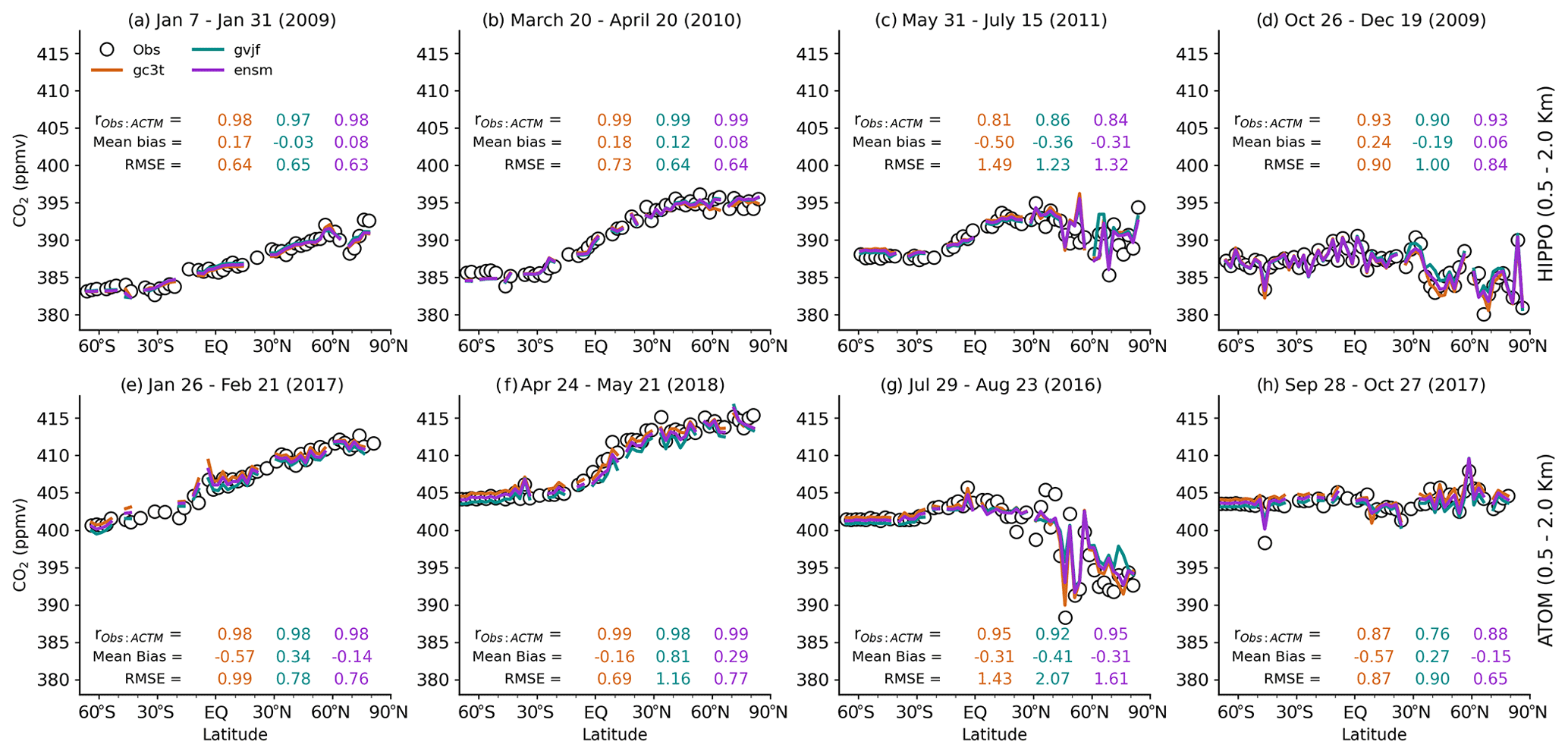
Figure 11 Observed and modeled meridional CO₂ distribution during HIPPO and ATom campaigns. We aggregate the observed and simulated mole fractions for the lower troposphere (between 0.5 and 2.0 km) at 2.5^∘ latitudinal bins. The correlation coefficient, mean model–observation bias, and root-mean-square error (RMSE) are also shown in each plot.

The ensm inversion shows the lowest mean bias and RMSE than the other two predicted simulations over most aircraft campaigns (Fig. 11, statistics on each panel for different fluxes identified by color). The comparison also indicates latitude- and season-dependent accuracy in the predicted fluxes. The NOAA aircraft observations show a high bias during boreal summer throughout the troposphere over the United States and Canada, implying possible seasonally dependent errors in posterior fluxes over these latitude regions (Fig. S7). When the aircraft data are over the high-latitude continental regions, the model–observation comparison suggests a stronger surface CO₂ sink is estimated by inversion compared to what is suggested by vertical profile gradients. HIPPO for July also shows negative model–observation mismatches near the surface (Fig. S6). But the mismatches turn positive in the higher altitudes, above about 1 km, and thus the model and observations averaged over 0–2 km are in much closer agreement (Fig. 11c). Based on these comparisons, the simulations from the ensemble mean of 16 inversion cases (ensm) show the lowest mean bias in comparison with gc3t or gvjf inversions and are suggested to be the most suitable flux estimation for quantifying the global land and ocean carbon sink on the timescale of the annual mean and its decadal trend.

Further, all available aircraft profiles, measured on a campaign basis or at regular intervals, are also used to evaluate the predicted fluxes (Table S4). Compared to NOAA vertical profiles of CO₂, model simulations agree well in the free troposphere (defined here between 2 and 8 km), with an average bias (averaged over 2000–2020) close to zero (Fig. S7, top panel: bias as a function of altitude, averaged over all sites). The inversions underestimate (∼ 1 ppm; Fig. S7, top panel) the observations within the boundary layer (between the surface and 2 km); however, the RMSE is higher (∼ 1 ppm) compared to that of the free troposphere. It could be because many of the NOAA aircraft profiles are over the United States (see the map inset in the middle row, left panel of Fig. S7), close to regional CO₂ sources.

Following the GCP budget evaluation method (Friedlingstein et al., 2020), Fig. 12 shows the mean bias over four latitude bands for three periods. The mean bias is calculated separately from all available aircraft data in obspack_co2_1_GLOBALVIEWplus_v6.1 (Fig. 12a–c) and 50 observation sites (Fig. 12d–f) used in the inversion (shown in Fig. 1). The biases show the dependency on latitude and are different for each inverse model case and provide information on biases in the surface fluxes (Gaubert et al., 2019; Houweling et al., 2015). All the three predicted CO₂ concentrations show the smallest bias (less than 0.1 ppmv) over the high southern latitudinal band for 2001–2010. However, for 2011–2020, predicted CO₂ concentrations show large positive (0.47 ± 0.47 ppm) and negative (−0.23 ± 0.47 ppm) bias for gc3t- and gvjf-predicted fluxes. The positive and negative biases for gc3t and gvjf inversions, respectively, are also consistent with the surface sites, which arise due to the biases in simulated CO₂ growth rates (an overestimated growth rate for gc3t for the positive budget imbalance (Fig. 5), the opposite being the case for the gvjf inversion with a negative budget imbalance). The mean biases turned from negative to large positive by moving from 0–45^∘ N averages to 45–90^∘ N averages. In contrast to aircraft observations, the surface sites show a large negative bias over 45–90^∘ N, consistent with the discussions earlier based on Figs. S5–S8. Overall, the ensm case shows consistent results in all three different time periods of this analysis, reiterating the appropriateness of the ensemble mean CO₂ fluxes for global (e.g., Fig. 5) and regional budget analysis (e.g., Table 4).

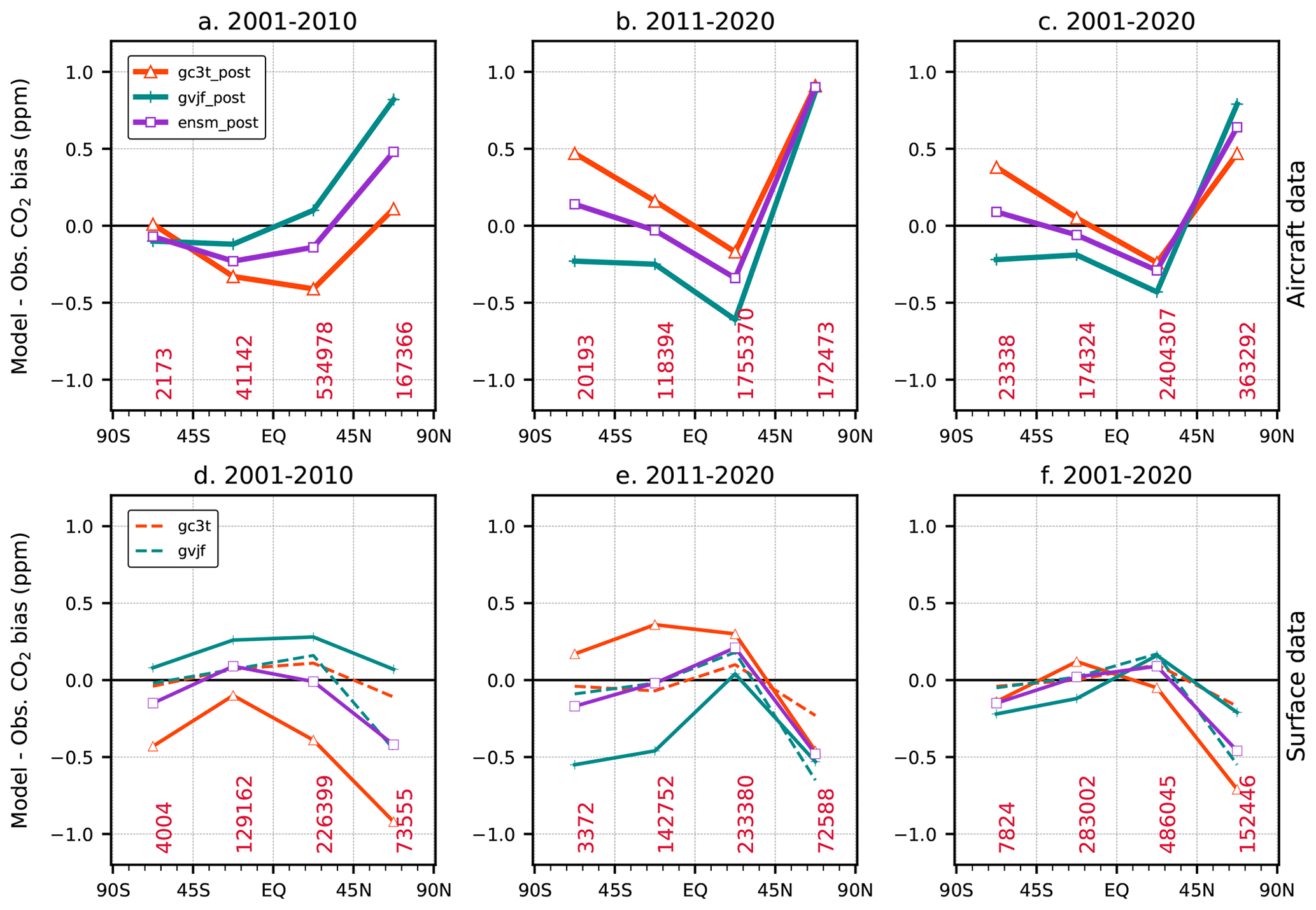
Figure 12 Evaluation of the atmospheric inversion products (solid lines; legend in panel a). The mean of model–observation differences is shown for four latitude bands of 45^∘ intervals in three time periods: (a, d) 2001–2010, (b, e) 2011–2020, and (c, f) 2001–2020. The simulations from three inversion cases are compared to independent CO₂ measurements made on board aircraft (a–c: top row) over various parts of the world between 2 and 8 km above sea level. Bottom row shows the model–observation differences for 50 surface sites that are used in the inversion (d–f) and mismatches between the a posteriori model (as obtained after optimizing regional sources by inversion) and CO₂ data (broken lines; legend in panel d). Land and ocean data are used without distinction. The number in each panel shows the total number of data points used for computing bias for each latitude bin. The observation data are taken from obspack_co2_1_GLOBALVIEWplus_v6.1 (Schuldt et al., 2021).

4 Conclusions

The terrestrial biosphere (2.58 PgC yr⁻¹) and ocean (1.54 PgC yr⁻¹) absorb about 46 % of the emissions due to fossil fuel and cement production (8.9 PgC yr⁻¹) in the period 2001–2020. The variability in these fluxes significantly affects the year-to-year variability of the carbon dioxide (CO₂) accumulation rate in the atmosphere. We estimated global and regional sources and sinks of carbon across the earth's surface, using observations and simulations of atmospheric CO₂. We tested the relative role of prior flux uncertainty (PFU) and model data uncertainty (MDU) on the land and ocean's global and regional carbon flux estimates. For this, we use a single transport model (JAMSTEC's MIROC4-ACTM) to estimate the global and regional carbon flux and associated uncertainty based on different prior fluxes (two land biosphere fluxes (CASA and VISIT + Fire) at 3-hourly intervals with distinct global total CO₂ sink strengths and two sea–air exchange fluxes (Takahashi and JMA)), choices of prior flux uncertainties (PFU: four cases), and representation of measurement data uncertainties (MDU: two cases). Based on different combinations of prior fluxes, PFU, and MDU, we run 16 ensembles of inversion cases using CO₂ measurements from a set of 50 sites spreading over the globe, and inversion results are analyzed for 2001–2020. The 16 ensemble members are averaged, and the result (ensm) is treated as the best estimate (i.e., a measure of central tendency) flux. The spread between the ensemble members provides us a reasonable measure of the inversion-estimated flux uncertainty but lacks the quantification of the roles of transport model uncertainty or the inherent errors in the measurements and the prior fluxes.

Although each inversion used common observation sites, there is still considerable uncertainty in the estimated fluxes due to the prior fluxes and uncertainties (PFU and MDU). On a global scale, the uncertainty in the predicted fluxes due to prior flux is relatively larger than that of PFU and MDU. However, at a regional scale, uncertainties due to priors and PFU and MDU are primarily comparable and drove inter-inversion disparity. The lack of constraints makes the tropical (Tropical America, South Asia, and Southeast Asia) and extratropical southern (Southern Africa, Oceania) land regions highly uncertain. The ensemble of inversions splits into a “near-neutral” group and a “strong source/sink” group based on the prior fluxes for the tropical and extratropical southern land regions. Overall, the prior flux differences have a negligible effect on the estimation of the global land total and ocean total sink but are significant at the regional scale.

The interannual variability in the land fluxes (driven mainly by ENSO) is much more considerable than in the ocean and tends to show greater consistency across the 16 inversion cases. The land flux seasonality is prominent in the Northern Hemisphere, with good agreement across the inversion ensemble cases. The ocean seasonality is slight and in less agreement relative to the magnitude of the seasonality of land fluxes. We comprehensively evaluated predicted fluxes by extensively comparing the simulated posterior CO₂ to independent CO₂ observations from several aircraft measurements by NOAA, CONTRAIL, HIPPO, ATom, and the NOAA MBL reference sites. The evaluation suggests that the ensemble mean of 16 inversion cases (ensm) is well suited (mean bias is found minimum) for quantifying the global land and ocean carbon sink. Thus, we used the ensm case (best estimate) for estimating the carbon fluxes and associated uncertainties.

In summary, our best estimate suggests that 22 %–33 % (16 %–18 %) of global CO₂ emissions from FFC have been offset by global land (ocean) carbon flux from 2001–2020. The land and ocean sink partitioning are estimated to be −2.27 ± 0.2 ( ± 1σ uncertainty on mean) and −1.46 ± 0.09 PgC yr⁻¹, respectively, for the period 2001–2009, and −2.85 ± 0.25 and −1.63 ± 0.17 PgC yr⁻¹, respectively, for the period 2010–2019 (without riverine export correction), which are in excellent agreement with the IPCC AR6 values (Table 3). The decadal mean values for the RECCAP are also in good agreement for North America, South America, East Asia, South Asia, and Oceania (Table 4). Note that the region boundaries and period of evaluations do not match perfectly between RECCAP-1 and our inversion for most regions.

Our analysis suggests that the most prominent land carbon sink in the Northern Hemisphere is located in Temperate North America (−0.59 ± 0.14 PgC yr⁻¹), followed by East Asia (0.49 ± 0.09 PgC yr⁻¹), Boreal North America (−0.38 ± 0.10 PgC yr⁻¹), and Russia (−0.35 ± 0.05 PgC yr⁻¹) for 2001–2020. Overall, our results suggest about 40 % of Temperate North America's (1.49 PgC yr⁻¹), 17 %–19 % of East Asia's (2.74 PgC yr⁻¹), 200 % of Boreal North America's (0.19 PgC yr⁻¹), and 80 % of Russia's (0.44 PgC yr⁻¹) CO₂ emissions from FFC are offset by carbon accumulation in their terrestrial ecosystems for 2001–2020. Further, the inversion suggests substantial oceanic CO₂ uptake in the North Pacific with a mean flux of −0.55 ± 0.05 PgC yr⁻¹, and also considerable CO₂ uptake is estimated for the Southern Ocean, where CO₂ uptake increased from −0.12 ± 0.07 PgC yr⁻¹ in 2001–2009 to −0.33 ± 0.06 PgC yr⁻¹ in 2010–2019. Overall, no area shows net carbon source from the land biosphere for recent decades (2010–2019).