the Creative Commons Attribution 4.0 License.
the Creative Commons Attribution 4.0 License.
 | 14 Jul 2022
Effective radiative forcing of anthropogenic aerosols in E3SM version 1: historical changes, causality, decomposition, and parameterization sensitivities
Wentao Zhang
Philip J. Rasch
Steven J. Ghan
Richard C. Easter
Xiangjun Shi
Yong Wang
Hailong Wang
Po-Lun Ma
Shixuan Zhang
Jian Sun
Susannah M. Burrows
Manish Shrivastava
Balwinder Singh
Yun Qian
Xiaohong Liu
Jean-Christophe Golaz
Xue Zheng
Shaocheng Xie
Wuyin Lin
Minghuai Wang
Jin-Ho Yoon
L. Ruby Leung
The effective radiative forcing of anthropogenic aerosols (ERFaer) is an important measure of the anthropogenic aerosol effects simulated by a global climate model. Here we analyze ERFaer simulated by the E3SM version 1 (E3SMv1) atmospheric model using both century-long free-running atmosphere–land simulations and short nudged simulations. We relate the simulated ERFaer to characteristics of the aerosol composition and optical properties, and we evaluate the relationships between key aerosol and cloud properties.
In terms of historical changes from the year 1870 to 2014, our results show that the global mean anthropogenic aerosol burden and optical depth increase during the simulation period as expected, but the regional averages show large differences in the temporal evolution. The largest regional differences are found in the emission-induced evolution of the burden and optical depth of the sulfate aerosol: a strong decreasing trend is seen in the Northern Hemisphere high-latitude region after around 1970, while a continued increase is simulated in the tropics. The relationships between key aerosol and cloud properties (relative changes between pre-industrial and present-day conditions) also show evident changes after 1970, diverging from the linear relationships exhibited for the period of 1870–1969. In addition to the regional differences in the simulated relationships, a reduced sensitivity in cloud droplet number and other cloud properties to aerosol perturbations is seen when the aerosol perturbation is large. Consequently, the global annual mean ERFaer magnitude does not increase after around 1970.
The ERFaer in E3SMv1 is relatively large compared to the recently published multi-model estimates; the primary reason is the large indirect aerosol effect (i.e., through aerosol–cloud interactions). Compared to other models, E3SMv1 features large relative changes in the cloud droplet effective radius in response to aerosol perturbations. Large sensitivity is also seen in the liquid cloud optical depth, which is determined by changes in both the effective radius and liquid water path. Aerosol-induced changes in liquid and ice cloud properties in E3SMv1 are found to have a strong correlation, as the evolution of anthropogenic sulfate aerosols affects both the liquid cloud formation and the homogeneous ice nucleation in cirrus clouds (that causes a large effect on longwave ERFaer).
As suggested by a previous study, the large ERFaer appears to be one of the reasons why the model cannot reproduce the observed global mean temperature evolution in the second half of the 20th century. Sensitivity simulations are performed to understand which parameterization and/or parameter changes have a large impact on the simulated ERFaer. The ERFaer estimates in E3SMv1 for the shortwave and longwave components are sensitive to the parameterization changes in both liquid and ice cloud processes. When the parameterization of ice cloud processes is modified, the top-of-model forcing changes in the shortwave and longwave components largely offset each other, so the net effect is negligible. This suggests that, to reduce the magnitude of the net ERFaer, it would be more effective to reduce the anthropogenic aerosol effect through liquid or mixed-phase clouds.
- Article
(18774 KB) - Full-text XML
-
Supplement
(23749 KB) - BibTeX
- EndNote


Variations in atmospheric composition have played an important role in causing the observed (historical) climate changes since the pre-industrial era. The concentrations of both greenhouse gases and aerosols have changed, with partially offsetting impacts on the Earth's radiative balance. Compared to greenhouse gases, the lifetime of aerosols is much shorter and the processes involved in the aerosol life cycle are more complex. In addition, aerosols affect the Earth's radiative balance not only by directly scattering and absorbing shortwave and longwave radiation but also by acting as cloud condensation nuclei and ice nuclei, hence changing the cloud formation process and cloud radiative forcing. Consequently, aerosols have been considered to be a group of the most uncertain forcing agents in the climate system (Penner et al., 2001; Forster et al., 2007; Boucher et al., 2013; Szopa et al., 2022; Forster et al., 2022).
Due to our incomplete knowledge of the aerosol-related processes and the limited spatial and temporal resolutions used by Earth system models or global climate models, most such models have rather simplified representations of aerosol lifecycles and their interactions with clouds, precipitation, and radiation. The complex and multi-scale aerosol-related processes are simplified and represented differently in the models, leading to large difference in the simulated aerosol properties (Textor et al., 2006) and their impacts on clouds (Zhang et al., 2016). As a result, the estimated anthropogenic aerosol effects in global climate models are quite uncertain for both the aerosol–radiation interactions (Schulz et al., 2006; Myhre et al., 2013) and aerosol–cloud interactions (Quaas et al., 2009; Ghan et al., 2016).
In an earlier study, Golaz et al. (2019) report that the present-day (average of 1995–2014) net (shortwave + longwave) effective radiative forcing of anthropogenic aerosols (ERFaer) in the atmosphere component of the Energy Exascale Earth System Model version 1 (E3SMv1) is about −1.65 W m−2. This value is outside the likely range of −0.63 to −1.37 W m−2 estimated from models participating in the Radiative Forcing Model Intercomparison Project (RFMIP, Smith et al., 2020) for the World Climate Research Programme Coupled Model Intercomparison Project Phase 6 (CMIP6, Eyring et al., 2016). Furthermore, E3SMv1's present-day ERFaer is close to the lower bound of the multi-model estimate from Bellouin et al. (2020), who report a 68 % likelihood range of −1.6 to −0.6 W m−2 and a 90 % likelihood range of −2.0 to −0.4 W m−2.
We note that E3SMv1 considers complex interactions between aerosols, clouds, and radiation (see Sect. 2.1.2), so the estimated ERFaer might be larger than those estimated in models with simplified aerosol treatment (Fiedler et al., 2019; Shi et al., 2019).
The large aerosol forcing in E3SMv1 appears to be one of the reasons why the model cannot reproduce the observed global mean temperature evolution in the second half of the 20th century, as suggested by the analysis of Golaz et al. (2019) based on a two-layer energy balance model. The present study complements that analysis by providing a comprehensive investigation of the aerosol forcing characteristics.
This study evaluates the ERFaer simulated by the E3SMv1 Atmosphere Model (EAMv1, Rasch et al., 2019) and relates the ERFaer to characteristics of the aerosol composition and optical properties. We also evaluate the relationships between key aerosol and cloud properties. Our analysis focuses on the following aspects.
-
The historical changes in aerosol properties and the regional differences in ERFaer are analyzed in Sect. 3. We investigate whether the historical changes in aerosol properties are consistent with the changes in the aerosol forcing and explore the temporal variations in different regions.
-
Second, following previous studies, we identify the most important aerosol, cloud, and radiation flux quantities and analyze the relationship between them (Sect. 4). The analysis focuses on the relative changes in these quantities based on the causality between them.
-
Possible causes of the strong ERFaer in E3SMv1 are explored in Sect. 5. The decomposition method of Ghan (2013) is used to quantify the contributions of individual forcing mechanisms (i.e., aerosol–radiation interaction, aerosol–cloud interaction, and residual effect) to the top-of-model (TOM) and surface ERFaer. The contribution of individual aerosol species to the overall ERFaer is quantified by perturbing one type of anthropogenic aerosol emission at a time.
-
The sensitivities of ERFaer to parameterization changes, including both formulation changes and parameter tuning, are discussed in Sect. 6. These parameterization changes were applied during the E3SMv1 development and some of them have been further tuned for an alternate configuration of E3SM (Ma et al., 2022).
-
Section 7 evaluates the impact of anthropogenic aerosols on the near-surface temperature through fast processes (in contrast to the slow processes involving ocean–sea ice responses to aerosol forcing).
The goal of the study is to better characterize and understand the strong ERFaer in E3SMv1 and hence provide insights to help constrain its value in future versions of the model. Descriptions of the model and simulations are provided in Sect. 2. The conclusions from the study are summarized in Sect. 8.
The model used in this study is the atmospheric component of the E3SMv1, often referred to as EAMv1. A comprehensive description of EAMv1 can be found in Rasch et al. (2019), and the representation of aerosol processes is documented in Wang et al. (2020); hence we only provide brief overviews here (Sect. 2.1). The simulations conducted and analyzed in this study are described in Sect. 2.2.
2.1 Model description
2.1.1 Overview
EAMv1 uses the High-Order Methods Modeling Environment (HOMME) spectral element dynamical core (Taylor and Fournier, 2010; Dennis et al., 2012) and a cubed-sphere mesh. The standard model resolution is used, which has approximately 100 km horizontal resolution, with 30 spectral elements (“ne30”). The model has 72 vertical layers (see Fig. 1 of Xie et al., 2018) and a top at approximately 0.1 hPa, with about 21 levels below 700 hPa and 26 levels above 100 hPa. The key physical processes considered include deep convection (Zhang and McFarlane, 1995), turbulence, shallow convection, and cloud macrophysics that are handled by CLUBB (Golaz et al., 2002; Larson et al., 2002; Larson, 2017), as well as cloud microphysics (Gettelman and Morrison, 2015; Wang et al., 2014), aerosol processes (see details in Sect. 2.1.2), and radiation (Iacono et al., 2008). More information about aerosol and cloud microphysics parameterizations is provided in the next subsection. Most parameterized physical processes use a time step of 30 min, which is also the time step for physics and dynamics coupling. A static (fixed sub-step length) or dynamic sub-stepping method is used by some parameterizations. For example, droplet activation and ice nucleation are coupled with CLUBB and cloud microphysical processes, with a coupling frequency of 5 min. The radiation time step is 1h. More details about process coupling and time stepping can be found in Zhang et al. (2018) and Wan et al. (2021). The evaluations of simulated large-scale circulation and clouds in EAMv1 are documented in Rasch et al. (2019), Xie et al. (2018), and Zhang et al. (2019). As summarized in Zhang et al. (2019), the major cloud biases in EAMv1 include
-
underestimated marine stratocumulus clouds at subtropical latitudes near the west coast of major continents,
-
underestimated thin cirrus clouds that result in a smaller longwave cloud radiative effect,
-
excessive low clouds over the Arctic, and
-
too much supercooled cloud liquid fraction.
All of these biases might affect the effective aerosol forcing estimate. EAMv1 is interactively coupled with a land surface model (Oleson et al., 2013), which also includes the dust emission calculation and the parameterization that considers the impacts of light-absorbing impurities (from black carbon and dust deposition) on surface snow–ice albedo (Wang et al., 2020).
2.1.2 Parameterization of aerosols and their interactions with radiation and clouds
Aerosol processes in EAMv1 (Wang et al., 2020) are represented by the Modal Aerosol Module (MAM) (Liu et al., 2012a, 2016). Major aerosol compositions are considered, including sulfate (SU), black carbon (BC), primary organic matter (POM), secondary organic aerosol (SOA), dust (DU), sea salt (SS), and marine organic aerosol (MOM). The aerosol size distribution is represented by four lognormal modes, with three soluble modes with mixed aerosol species and one primary carbon mode for BC and POM (see Fig. 2 of Wang et al., 2020). Aerosols are assumed to be internally mixed within each mode but externally mixed between different modes. MAM prognoses both the interstitial aerosols (particles suspended in the air and not in cloud droplets) and cloud-borne aerosols (particles in cloud droplets). The model evaluation of present-day aerosol properties in EAMv1 is documented in Wang et al. (2020). The model representation and evaluation of dust and marine organic aerosols are documented in Burrows et al. (2022) and Feng et al. (2022).
The aerosol optical properties are parameterized based on the study by Ghan and Zaveri (2007), which approximates the calculation using analytic functions of the mode radius and refractive index of wet particles. The refractive indices for individual aerosol compositions are from Hess et al. (1998), except that the refractive index for BC is taken from Bond and Bergstrom (2006). The volume mixing rule is assumed when calculating the volume-mean wet refractive index for aerosol modes with mixed compositions. The Köhler-theory-based water uptake scheme is used to calculate the wet particle size in each mode based on the predicted aerosol composition and hygroscopicity, as well as the relative humidity with respect to water (RHw) in the clear-sky portion of the grid box. The hygroscopicity values for individual compositions can be found in Table 1 of Burrows et al. (2022). In MAM, an RHw ceiling of 98 % is applied for the aerosol water uptake calculation.
For liquid cloud formation, soluble aerosols can act as cloud condensation nuclei and get activated to form cloud droplets in existing or newly formed clouds. The Abdul-Razzak and Ghan (2000) activation scheme is used, which parameterizes the aerosol activation (or droplet nucleation) based on the subgrid updraft velocity and the aerosol properties (especially for dry size and hygroscopicity) in each mode. Instead of calculating the aerosol activation with a spectrum of updraft velocities as in Ghan et al. (2001), MAM uses a so-called characteristic subgrid updraft velocity to simplify the calculation, which is parameterized as a function of the turbulent kinetic energy (TKE) prognosed by CLUBB. A lower bound of 0.2 m s−1 (inherited from the CAM5.4) is applied to the characteristic subgrid updraft velocity1 in order to compensate for the potentially underestimated turbulence strength due to unresolved processes (e.g., cloud-top radiative cooling). No minimum cloud droplet number concentration is applied in E3SMv1. The activation process is coupled with an explicit vertical diffusion scheme with dynamical sub-stepping, which handles the vertical diffusion transport of all aerosol species and the cloud droplet number.2
For mixed-phase clouds, E3SMv1 uses a parameterization based on classical nucleation theory (CNT). The deposition, immersion, and contact freezing of natural dust and BC particles are considered based on a PDF (probability density function) representation of contact angles for those particles (Wang et al., 2014). The initial ice particle size is assumed to be the same as the mean cloud droplet size. Among the different heterogeneous ice formation mechanisms considered in E3SMv1 for mixed-phase clouds, the immersion freezing of dust is the dominant source for ice formation. The contributions from other ice nucleation pathways (the deposition and contact freezing of dust and the immersion freezing of BC) are much smaller. In addition, all the droplets are assumed to homogeneously freeze when ∘C (note that this is different from the homogeneous nucleation of sulfate aerosols), with an initial size of 25 µm. The previously used Meyers scheme (Meyers et al., 1992) for deposition and condensation freezing as well as the contact nucleation scheme (Young, 1974) are optional and are explored as a sensitivity test in this study (see Sect. 6).
For cirrus cloud formation ( ∘C), the homogeneous freezing of sulfate aerosols and heterogeneous immersion freezing on mineral dust are considered using the Liu and Penner (2005) ice nucleation scheme. For both nucleation mechanisms, an initial ice particle size of 10 µm is assumed. As for droplet nucleation, the ice nucleation scheme also uses the characteristic updraft velocity (as a function of TKE), with a lower bound of 0.2 m s−1. Sulfate aerosols (or sulfate solution droplets) in the Aitken mode with a diameter larger than a threshold are considered ice-nucleating aerosols for the homogenous ice nucleation. This size threshold was first introduced in the CAM5 model to better reproduce observations (Neale et al., 2010, page 135), and it was set differently in various modeling studies. For example, a threshold size of 100 nm was used in the CAM5 model, while in some sensitivity studies (e.g., Liu et al., 2012b; Zhang et al., 2013; Shi et al., 2015), all Aitken-mode particles are considered to be potential ice-nucleating aerosols in cirrus clouds. E3SMv1 inherited this treatment and further tuned the threshold mainly based on the evaluation of cloud fraction and cloud radiative forcing. For the E3SMv1 CMIP6 experiments and the reference model used in this study, a threshold size of 50 nm is used (Golaz et al., 2019). We discuss this parameter sensitivity in Sect. 6.
2.2 Simulations
Ma et al. (2022)Khairoutdinov and Kogan (2000)Meyers et al. (1992)(Wang et al., 2014)Table 1List of simulation configurations. Note that for SOA, the 3D formation rates calculated based on Shrivastava et al. (2015) are applied as emissions in E3SMv1.
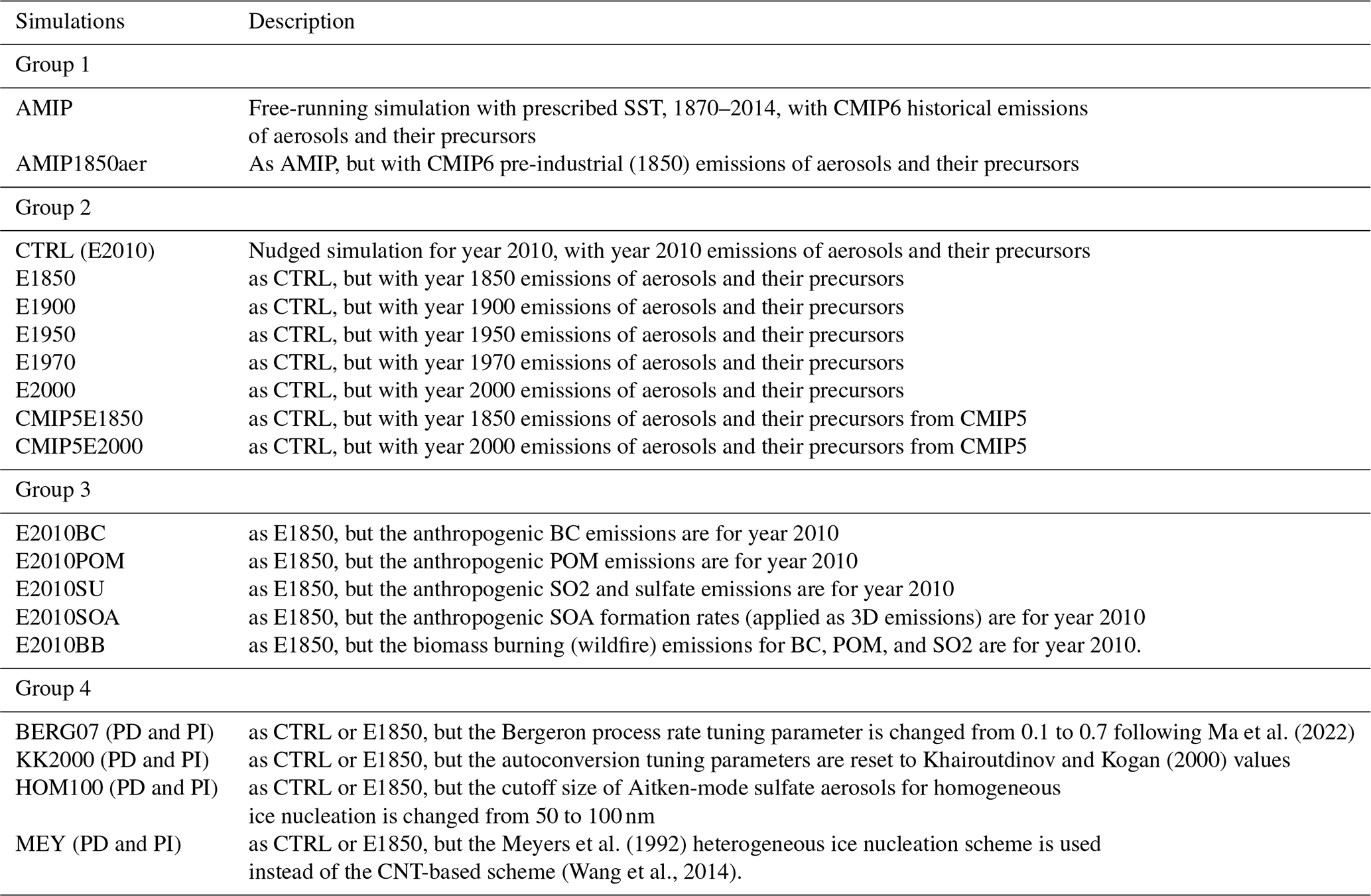
Four groups of simulations are analyzed in this study (see Table 1). First, we further analyze the atmosphere-only simulations from Golaz et al. (2019) with prescribed historical sea surface temperature (SST) and sea ice concentration for the years 1870–2014. In the reference simulation ensemble (AMIP), transient–historical anthropogenic and biomass burning–biofuel emissions as well as other forcings (e.g., concentrations of greenhouse gases) are prescribed using the CMIP6 emission data (Hoesly et al., 2018) with additional corrections by Feng et al. (2020). In the second simulation ensemble (AMIP1850aer), the anthropogenic and biomass burning–biofuel emissions are kept at the 1850 level (also from CMIP6). Dimethyl sulfide (DMS) emissions for three time slices (1850, 2000, and 2100) are available from a coupled model simulation, with detailed representation of DMS formation in seawater (Wang et al., 2018), and are linearly interpolated for other periods. Dust, sea salt, and marine organic aerosol emissions are calculated interactively in all the simulations analyzed in this study based on the simulated surface winds (frictional velocity for dust) and other surface quantities from the land and ocean components. We take the difference between AMIP and AMIP1850aer to obtain the temporal evolution of anthropogenic aerosol properties, including mass burden, cloud condensation nuclei (CCN) number, and optical depth, as well as the transient ERFaer. Each set of simulations has three ensemble members, and the ensemble-averaged fields are used for analysis.
The AMIP-type simulations from Golaz et al. (2019) only include limited monthly mean output for aerosol-related quantities, so additional output data are needed for more detailed analysis. Due to limited computational resources, we rely on shorter simulations that are nudged towards reanalysis data for the additional three simulation groups. Nudged simulations help identify the aerosol forcing signal (i.e., spatial pattern) over shorter time periods (e.g, a specific year). See further discussions later in this section.
The second group includes nudged simulations with emissions of anthropogenic and biomass burning–biofuel aerosols as well as their precursors fixed to a specific year. We picked six time slices to represent pre-industrial (E1850), early industrial (E1900), mid-industrial (E1950), European peak industrial (E1970), near-present (E2000), and present (E2010, also as the nudged CTRL) conditions. By taking the difference between E1850 and all other simulations in this group, we derive the anthropogenic aerosol effects in each (emission) period and investigate the regional shifts of the aerosol forcing pattern. In addition to using the CMIP6 emissions, we also performed simulations using the CMIP5 emissions (Lamarque et al., 2010). As shown in Table 2 and Fig. S5 (in the Supplement), using the CMIP5 emissions results in a slightly smaller ERFaer estimate in E3SMv1.
The third group consists of simulations with 1850 aerosol emissions, but with individual aerosol species emission (or 3D production rates for SOA) set to the present-day (2010) value. Again, by taking the difference between E1850 and simulations in this group, the aerosol forcing by individual aerosol species can be derived. For DMS, the global mean difference between DMS emissions in 1850 and 2010 (interpolated) is very small (<1%), and sensitivity simulations show that it has a negligible impact on the simulated ERFaer. Therefore, the result for DMS is not included here. Dust, sea salt, and marine organic aerosols are not considered to be forcing agents, since their emissions are calculated online and/or interactively in the model and are mainly affected by the natural variability and feedback of the perturbed climate and Earth system.
The last group includes simulations similar to the nudged CTRL and E1850, but with the cloud microphysics parameterization switched back to older schemes or tuned with a different parameter. Several pairs of simulations were performed with both present-day (PD) and pre-industrial (PI) aerosol emissions to estimate the anthropogenic aerosol effects.
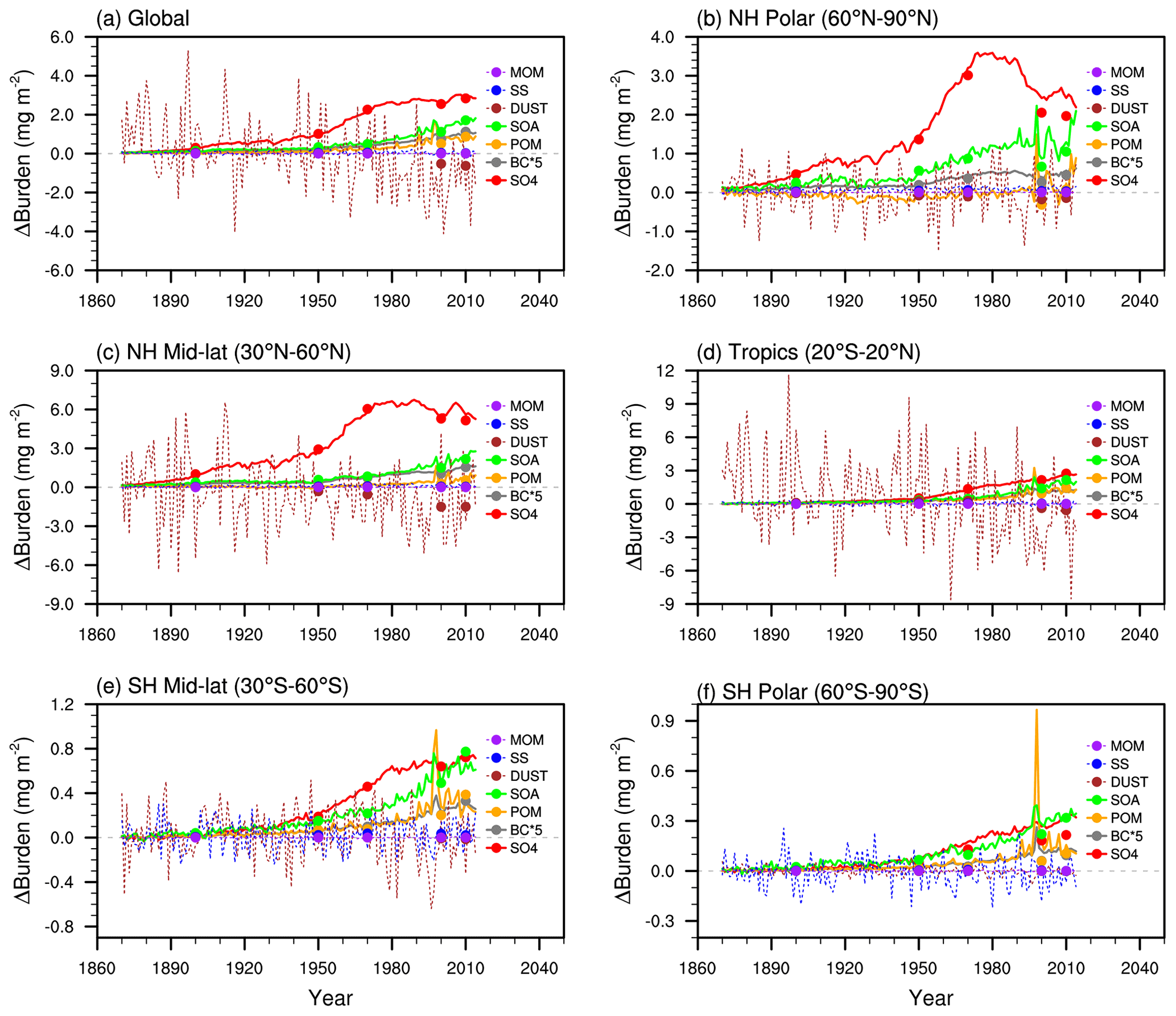
Figure 1Temporal variations of global and annual mean aerosol burden differences between simulations with transient and pre-industrial (1850) aerosol emissions. Solid lines indicate aerosol species that are directly influenced by anthropogenic aerosol emissions (SO4, BC, POM, SOA), and dotted lines indicate natural aerosols (DUST, SS, MOM) that are mainly driven by surface winds. Dots indicate results from the short nudged simulations. Note that for clarity, the BC Δburden is scaled by a factor of 5.
Since the large-scale circulation is constrained, nudging can help distinguish the signals (e.g., caused by changes in external forcings) from the noises caused by chaotic model responses to forcing or parameterization changes (Kooperman et al., 2012; Zhang et al., 2014). We only nudge horizontal winds in our simulations because it is better not to constrain the thermodynamical response of meteorological fields to aerosol effects. Also, earlier studies show a negative impact of temperature and humidity nudging on the modeled climate (Zhang et al., 2014; Lin et al., 2016; Sun et al., 2019), which will make the forcing estimate inconsistent with that estimated using free-running simulations. For all the nudged runs, we nudge the horizontal winds towards the ERA-Interim reanalysis data, with a relaxation timescale of 6 h. Since the vertical interpolation–extrapolation of reanalysis data to model vertical grids might have large errors near the surface, nudging is not applied in the lowest two layers. In the layer next to the no-nudging layers, the nudging relaxation time is doubled (weaker nudging compared to the layers above with full nudging strength). Each nudged simulation is 15 months long and the results from a whole year (after a 3-month spin-up) are used for analysis.
We note that since the horizontal winds are constrained in the nudged simulations, the anthropogenic aerosol effect on the large-scale circulation is greatly diminished. As we will show later, for global mean or regional mean (over a large area) estimates, the nudged simulations provide similar ERFaer estimates as the free-running simulations.
Before showing the effective aerosol forcing, we first analyze the simulated historical changes in anthropogenic aerosol burdens (vertical integration of aerosol mass) over the simulation period (1870–2014). Here, we define the anthropogenic change in a certain quantity (denoted as Δ, e.g., aerosol burden, optical depth, and radiative fluxes) as the differences between the modeled quantities in simulations with transient historical forcing and the pre-industrial forcing (year 1850) for aerosols and their precursors. Note that the anthropogenic change we define here also includes the contribution from biomass burning emissions, which is consistent with the IPCC (Intergovernmental Panel on Climate Change) definition of “anthropogenic” in a radiative forcing context.
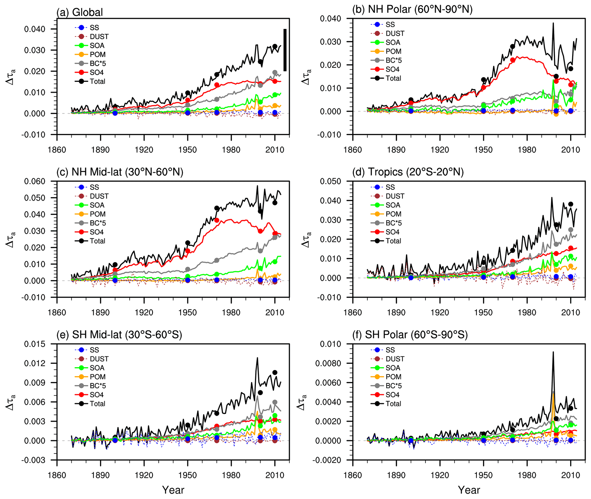
Figure 2Similar to Fig 1, but for anthropogenic aerosol optical depth at 0.55 µm (total and individual components). Solid lines indicate aerosol species that are directly influenced by anthropogenic aerosol emissions (SO4, BC, POM, SOA), and dotted lines indicate natural aerosols (DUST, SS, MOM) that are mainly driven by surface winds. Dots indicate results from the short nudged simulations. The black vertical bar in panel (a) shows the estimated range of total Δτa by Bellouin et al. (2020). Note that the BC values are scaled by a factor 5 for easier comparison. See Sect. 3.1 for details.
3.1 Changes in anthropogenic aerosol burden and optical depth
Figure 1 shows the historical changes in global and regional mean anthropogenic aerosol burden (Δburden) for different compositions. In addition to the results from AMIP-type simulations, we also show the nudged simulations for 5 selected years (shown as dots). Overall, the results from the nudged simulations agree very well with those from the AMIP-type simulations in terms of both historical variations and regional differences of Δburden.
For aerosols with anthropogenic sources (i.e., sulfate, BC, POM, SOA), the global mean anthropogenic burden (Fig. 1a) shows an overall increase during the simulation period (1870 to 2014). The burden of anthropogenic sulfate shows largest change, followed by that of SOA and POM (note that the BC Δburden is scaled by a factor of 5 in Fig. 1). There are large regional differences in Δburden. For example, the anthropogenic sulfate burden in the Northern Hemisphere (NH) polar region (60–90∘ N) peaks in the 1970s and decreases by about 50% in the year 2010 compared to the peak value (Fig. 1b). This is consistent with the emission reduction of air pollutants in Europe and North America where the legislation for clear air was implemented from the 1970s (Sliggers and Kakebeeke, 2004), while in the tropics (20∘ S–20∘ N), the sulfate burden continues to increase (Fig. 1d).
The carbonaceous aerosols are not only affected by the anthropogenic aerosol sources (e.g., from industrial and transport sectors), but also by the biomass burning emissions. In addition to the gradual increase in time, there are several intermittent spikes in the anthropogenic aerosol burden change. For example, the global biomass burning emission is largest in 1997 (van der Werf et al., 2017), an extreme El Niño year, and it contributes to a large increase in carbonaceous aerosol burden change. The impact of biomass burning emissions is more evident in cleaner areas like SH midlatitude and polar regions (Fig. 1e, f). Similar increases are also present in the NH polar region, where biomass burning emissions increase significantly after 2011 (especially over boreal North America and boreal Asia; see Fig. 9 of van der Werf et al., 2017).
The change in dust aerosol burden caused by the anthropogenic aerosol effect has large interannual variabilities, and there is a small decreasing trend after about 1950, indicating that anthropogenic aerosols can indirectly affect the dust life cycle, especially in the tropics and NH midlatitude region (Fig. 1d, c). To understand what causes the decreasing trend in the dust aerosol burden, the dust mass budget is evaluated using the nudged simulations (the impact of interannual variability in the AMIP simulations can be avoided). We find that the small decreasing trend is mainly caused by slightly weakened dust emission in simulations with increased anthropogenic emissions. Compared to the simulation with 1850 emissions, the global mean dust emission rate decreased by 2 %–3 % in the simulations with emissions after 1970. In the nudged simulations, we only weakly constrain the large-scale horizontal winds, so the near-surface winds can still be affected by stability changes in the lower troposphere. The slightly weakened dust emission is very likely due to the changed surface winds caused by anthropogenic aerosols through changes in the atmospheric stability in the lower troposphere (Jacobson and Kaufman, 2006; Baró et al., 2017). The dust wet removal rate also decreases with increased anthropogenic emissions, suggesting that the impact of anthropogenic aerosols on dust wet scavenging (through coating) is less important in our model compared to the dust emission changes.
Changes in sea salt and marine organic aerosol burdens are small (only evident in SH midlatitude and polar regions) and also have large interannual variations. Both sea salt and marine organic aerosol emissions are dependent on surface winds, SST, and the ocean fraction. The large interannual variations (from AMIP simulations) are mainly caused by changes in surface winds in combination with sea ice concentration and SST changes in different years. For the nudged simulations, since the large-scale winds are constrained and single-year SST and sea ice concentrations are used, the changes in sea salt and marine organic aerosol burden are very small.
Figure 2 shows the historical changes in global and regional mean anthropogenic aerosol optical depth (Δτa) for the total and individual aerosol components. Again, we see consistent results between the estimates by AMIP-type simulations and nudged simulations constrained to the same large-scale wind fields but with different years of emission input. The total Δτa (black) shows an overall increase during 1870–2014, but with large interannual variations. The interannual variability in total Δτa is caused by changes in dust aerosols and by changes in carbonaceous aerosols (BC, POM, SOA) affected by fluctuations in biomass burning emissions and by changes in dust aerosols. Compared to the multi-model estimates for Δτa (0.015–0.04) by Bellouin et al. (2020) based on multiple global model estimates (vertical bar in Fig. 2a), the estimated present-day Δτa in E3SMv1 (about 0.03 around the year 2010) is well within the range.

Figure 3Contribution of sulfate, BC, POM, and SOA to anthropogenic aerosol optical depth (excluding dust, sea salt, and marine organic aerosols) in 1970, 2000, and 2010. Numbers in the panel title are the total anthropogenic aerosol optical depth (Δτa,ant = Δτa,SO4 + Δτa,BC + Δτa,POM + Δτa,SOA). Results are calculated using the AMIP simulations. For example, the contribution from sulfate is calculated as . See Sect. 3.1 for details.
Δτa of individual aerosol compositions shows similar temporal variations and regional differences as seen in Δburden (Fig. 1). It can be clearly seen that after 1970, both sulfate burden and sulfate Δτa over NH polar and NH midlatitude regions decrease significantly, while for carbonaceous aerosols, there is an overall increase in burden and Δτa. Figure 3 provides a more quantitative comparison of the contributions of sulfate, BC, POM, and SOA to the total anthropogenic Δτa (excluding dust and sea salt). The contribution of carbonaceous aerosols to total anthropogenic Δτa increases from 27 % (BC 8 %, POM 6 %, and SOA 13 %) in 1970 to 48 % (BC 11 %, POM 13 %, and SOA 24 %) in 2000 and 50 % (BC 12 %, POM 10 %, and SOA 28 %) in 2010. Since carbonaceous aerosols are less hygroscopic compared to sulfate in the model, their increased contribution to aerosol mass (burden) will decrease the mean hygroscopicity of the aerosol particles and thus affect the optical property and the ability to be activated to cloud droplets. As will be shown later, the changes in the relative contribution of different types of anthropogenic aerosol components will have an impact on the relationship between Δτa, CCN (cloud condensation nuclei) concentrations, and droplet concentrations (Nd).
3.2 Historical changes in ERFaer
Figure 4 shows the historical changes in global and regional mean ERFaer (ΔF) for the net (dark grey), shortwave (blue), and longwave (red) components. The global mean shortwave ΔF is mostly negative and the largest negative forcing (about −2.6 W m−2) first appears around 1980. In contrast, the longwave ΔF is overall positive, with the largest forcing of about 1.0 W m−2. After 1980, the global mean ΔF does not show a clear increasing or decreasing trend, but there are fluctuations caused by interannual variations. Similar to the Δburden and Δτa results, we can see large regional differences in the temporal evolution of ΔF. The overall increasing or decreasing trend in ΔF resembles the changes in sulfate Δburden and Δτa, especially for NH midlatitude and polar regions.
Compared to ΔF estimated by CMIP6 RFMIP models (Smith et al., 2020), which adopt year 2014 emissions as present-day conditions, the shortwave and longwave ΔF estimated by E3SMv1 are barely within the max-to-min range in the CMIP6 RFMIP model estimates (thin vertical bars) but outside the 1 standard deviation around the mean estimate (thick vertical bars). For the net ΔF, the E3SMv1 estimate is even larger than the max–min range of the multi-model estimates, since the large shortwave and longwave ΔF estimates from CMIP6 are from the same model and the net change is relatively small.
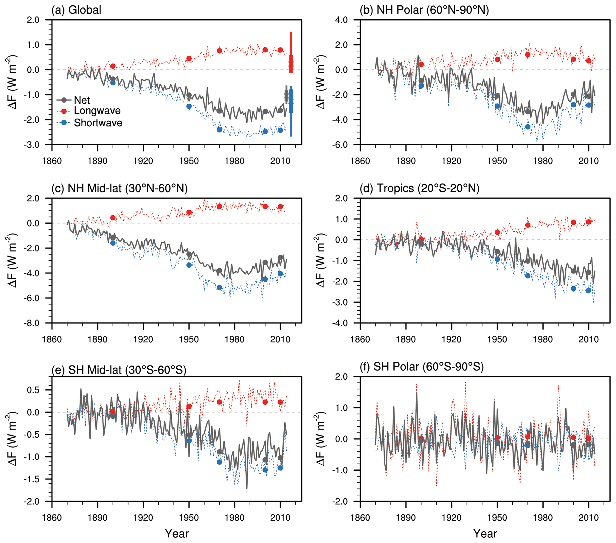
Figure 4Temporal variations of global and annual mean ERFaer (W m−2) derived from the differences between simulations with transient and pre-industrial aerosol emissions. Solid lines indicate net ERFaer, and dotted lines indicate the shortwave (blue) and longwave (red) components. Dots indicate results from the short nudged simulations. The cross and the thick and thin vertical bars show the mean, standard deviations, and max–min ΔF estimated by CMIP6 RFMIP models (Smith et al., 2020). See Sect. 3.2 for details.
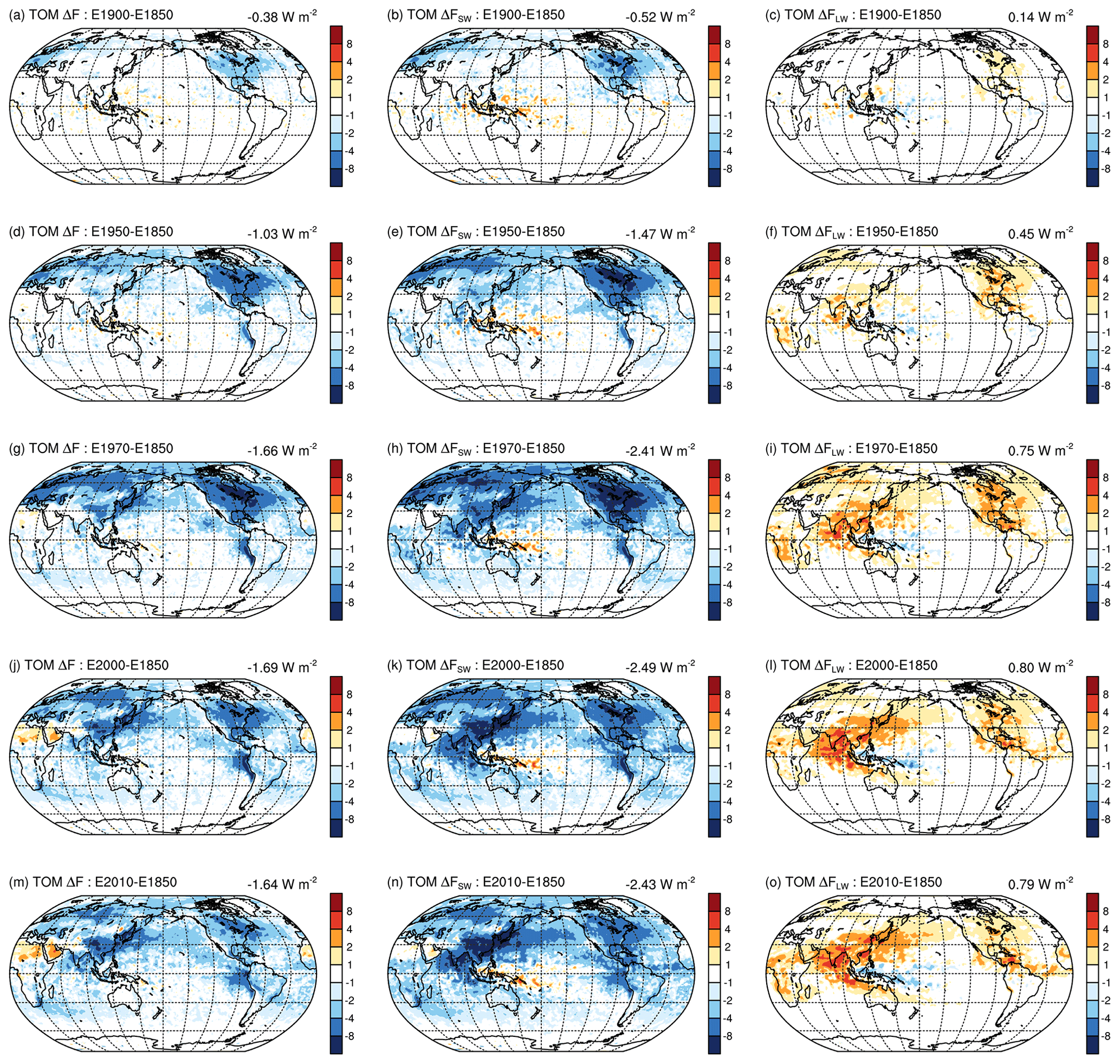
Figure 5Geographical distributions of annual mean net (left), shortwave (middle), and longwave (right) ERFaer (ΔF, W m−2) at the top of the model (TOM) estimated for different time slices using nudged simulations. Numbers shown on the top right of each panel are global mean values. For a given time slice, the CMIP6 aerosol emissions for the corresponding year are used. Simulations are described in Table 1, and “E2010” represents the CTRL simulation. See Sect. 3.2 for details.
As for Δburden and Δτa, the ΔF values estimated by the nudged simulations (dots in Fig. 4) are very similar to the estimates from the AMIP-type free-running simulations (lines). Therefore, in the following we mainly use results from the nudged simulations to discuss the regional forcing shifts, forcing decomposition (Sect. 5), and sensitivity to parameterization changes (Sect. 6). Note that since the large-scale circulation is constrained, the estimated ERFaer is mainly affected by fast processes associated with interactions between aerosol, cloud, precipitation, and radiation.
Figure 5 shows the geographical distributions of ΔF for different time slices estimated based on several pairs of nudged simulations (group 3 in Table 1) with emissions set to 1850 or a specific year (1900, 1950, 1970, 2000, or 2010). The corresponding changes in aerosol optical depth (AOD) and column-integrated number concentrations of CCN (at 0.1% supersaturation) and cloud droplets are shown in Figs. S8, S9, and S10.
In 1900, relatively large ΔF appears over western and northern Europe, North America, and the downwind regions. We see an overall increase in the magnitude of ΔF in 1950 (about a factor of 3 larger than the 1900 value), but the regions with large ΔF are still very similar as in 1900. The ΔF over western and northern Europe and North America peaks in 1970. Afterwards, the largest ΔF gradually shifts to East Asia. The estimated ΔF values for the years 2000 and 2010 are very similar, although the forcing over western and northern Europe and North America is further reduced in 2010.
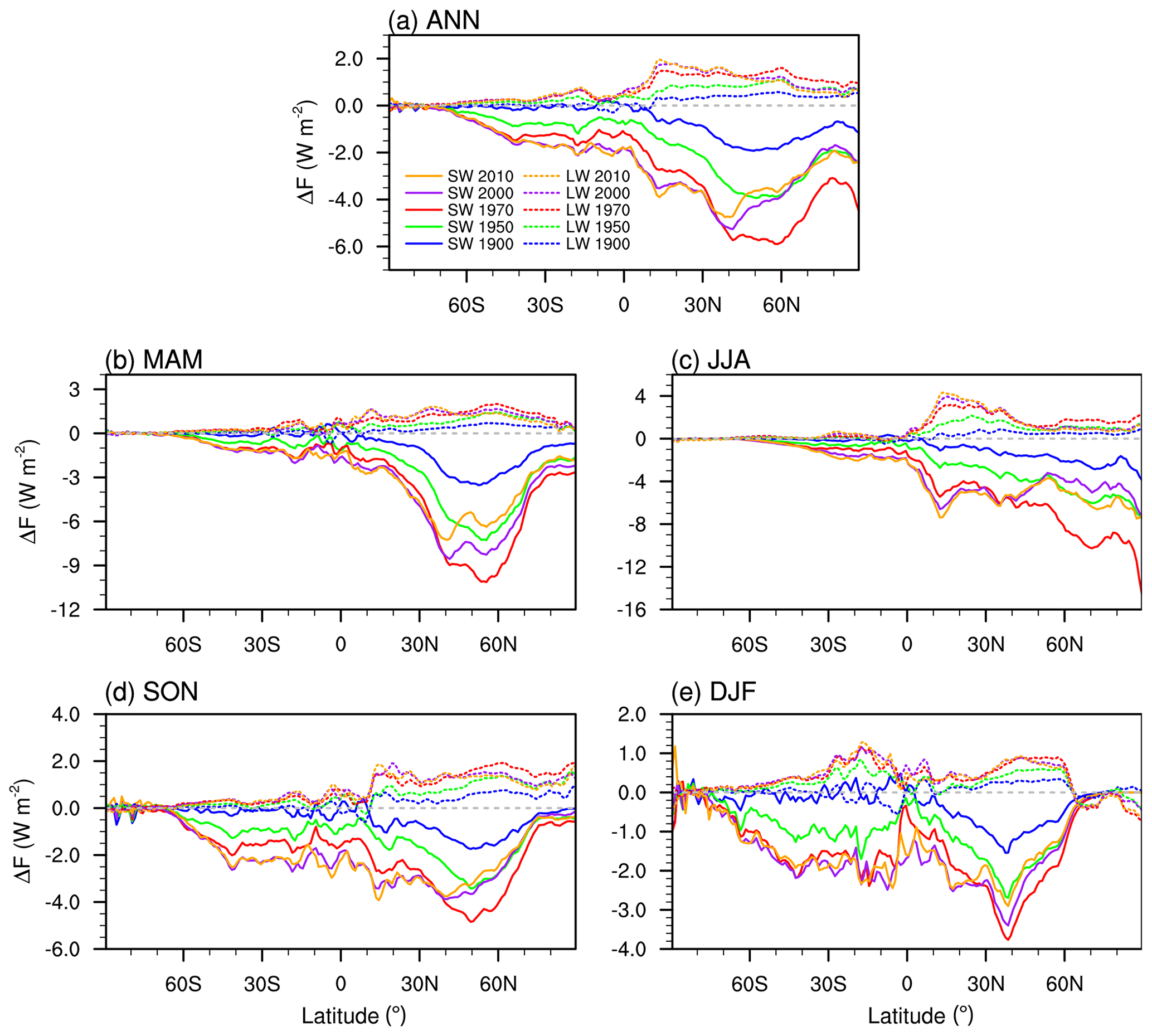
Figure 6Annually and seasonally averaged zonal mean top-of-model ΔF (W m−2) estimated for different time slices (emission years) indicated by different colors. Solid lines show the shortwave ΔF and dotted lines the longwave ΔF. In JJA, the shortwave ΔF for 1970 (relative to 1850) is about −14 W m−2 near the North Pole. See Sect. 3.2 for details.
Figure 6 clearly shows that ΔF has strong seasonal variations. The global mean ΔF is larger in boreal summer (June–July–August) and spring (March–April–May), mainly due to stronger oxidations of SO2 and higher sulfate concentrations in these seasons. Also, both the annual and seasonal averaged zonal mean ΔF fields have a regional shift of larger aerosol forcing from NH high-latitude regions in 1970 to the tropics and subtropics in 2000 and 2010, mainly due to regional changes in anthropogenic emissions. The largest changes in the NH polar region appear in boreal summer, from about −8 W m−2 in 1970 to −4 W m−2 in 2010.
In winter, shortwave ΔF in the NH polar regions is close to zero due to very small incoming shortwave radiation. As is shown later, the increased liquid water path by anthropogenic aerosol effects results in a positive (longwave) radiative forcing at the surface, which causes surface temperature to increase in addition to the greenhouse warming.
The impacts of aerosol perturbations on the top-of-model radiative flux changes involve many processes related to aerosol and cloud microphysics. Previous studies (Quaas et al., 2009; Ghan et al., 2016; Bellouin et al., 2020) have summarized the key causal relationships that determine the aerosol effect through interactions with radiation and clouds. These relationships are often expressed in the logarithmic form of , since most processes involved in aerosol–cloud interactions are more sensitive to a relative change (between pre-industrial and present-day conditions) in quantity than the absolute change (Carslaw et al., 2013; Bellouin et al., 2020). We follow the conventional expressions as used in Ghan et al. (2016) and Bellouin et al. (2020). In the following discussions, Δln X is the relative change in X (spatial and temporal mean) between PD and PI simulations, and it is calculated as 3 .
In earlier studies, some aerosol and cloud quantities are sampled at certain locations or under selected conditions based on their role in the physical processes or the consideration for comparing with satellite retrievals. For example, the cloud-base values of CCN (e.g., 1 km above the surface) and the cloud-top values of cloud droplet number concentrations (Nd) are often used (e.g., Quaas et al., 2009; Ghan et al., 2016; Zhang et al., 2016). Furthermore, to focus on the analysis on certain types of clouds, in some studies (e.g., Ghan et al., 2016; Gryspeerdt et al., 2020) these quantities are conditionally sampled only when some criteria are met (e.g., when cloud-top temperature is larger than a threshold value). For such analysis, high-frequency output data for the related aerosol and cloud properties are needed unless the model can conditionally sample data online and process them accordingly (Wan et al., 2022).
It should be noted that in our AMIP simulations, not all the quantities needed for such analysis are available or available at the required frequency (e.g., 3-hourly). Therefore, for some quantities (such as for CCN and Nd), we use the available column-integrated quantities sampled as monthly mean fields for the analysis using AMIP simulations. For the nudged simulations, both monthly mean output and high-frequency data sampled under required conditions (as in Ghan et al., 2016) are available, so we use both and evaluate whether the results are sensitive to the data sampling methods.
4.1 Relationships between Δln τa (or Δτa) and other quantities
Figure 7 shows the relationships between simulated changes in AOD (Δτa, Δln τa) and key cloud and radiative flux properties. The global annual mean total AOD (τa, Fig. 7a) from the AMIP simulation increased (almost linearly) from about 0.110 to 0.145 during the simulation period. Compared to the AMIP simulation (small dots), τa is consistently smaller in the nudged simulations with anthropogenic emissions for different years (shown as bigger markers). This is mainly caused by the slightly weakened dust emission when reanalysis nudging is applied (Timmreck and Schulz, 2004; Sun et al., 2019). Although we do not apply nudging in the surface layer, the simulated surface winds and dust emission fluxes are still affected by the nudging in upper layers (see Fig. 18 in Sun et al., 2019). The estimated present-day (year 2010) τa is well within the range of multi-model estimates (0.12–0.16 from Ghan et al., 2016, and 0.13–0.17 from Bellouin et al., 2020, shaded area in Fig. 7). The simulated anthropogenic AOD (Δτa) shows a similar increase during the simulation period. The estimated present-day Δτa (∼0.03) in E3SM is also well within the range of multi-model estimates.

Figure 7Relationships between simulated anthropogenic AOD (Δτa) and present-day total AOD (τa), relative (PD-PI) changes in AOD (Δln τa) and in the column-integrated CCN at 0.1 % supersaturation (ΔlnCCN0.1 %), Δln τa and relative changes in the column-integrated Nd (Δln Nd), and Δτa and changes in clear-sky shortwave radiation (ΔFSW,clear). . Dark grey dots indicate estimated values from AMIP PD/PI simulations for the years 1870–1969, while red dots are the estimated values for the years 1970–2014. Each dot represents the ensemble-averaged global annual mean field for a certain year. Blue markers show the estimates based on nudged simulations. The orange square shows the nudged simulation results averaged from conditionally sampled high-frequency data following Ghan et al. (2016), wherein CCN (at 0.3 % supersaturation) and Nd are sampled below 1 km and at the top of liquid clouds. Grey areas in panels (a, d) indicate the multi-model estimated range from Bellouin et al. (2020) and in panels (b, c) the multi-model estimated range from Ghan et al. (2016). See Sect. 4.1 for details.
The relationship between Δln τa (Δτa/τa) and ΔlnCCN0.1% is shown in Fig. 7b. They have a quasi-linear correlation before 1970 (grey dots). As indicated by the changed slope, the increase in ΔlnCCN0.1 % is weakened as Δln τa further increases after 1970 (red dots). Results from the nudged simulations show very similar changes. When sampling the data conditionally (cloud-top temperature ∘C) at high frequency, the result (shown as an orange square in Fig. 7b, c, d) is similar to that derived using the monthly mean data available, and it is within the multi-model estimated range in Ghan et al. (2016). Δln τa and ΔlnNd also show a quasi-linear correlation before 1970, but the slope changes sign for samples after 1970. This is likely related to the fact that there is a continuous increase in anthropogenic carbonaceous aerosols in most regions (that increases τa) but decreased or stabilized anthropogenic sulfate aerosols in the NH high-latitude and midlatitude regions. We note that the Nd changes in response to CCN changes are different between individual regions (see Figs. S9 and S10 and discussions in Sect. 4.2). In addition, the droplet nucleation is also dependent on the maximum supersaturation in a rising cloud parcel, which is parameterized based on the ambient meteorological conditions (e.g., vertical mixing and subgrid updraft velocity).
Following Bellouin et al. (2020), Fig. 7d shows the relationship between Δτa and the changes in clear-sky shortwave radiation (ΔFSW,clear). ΔFSW,clear magnitude increases with increasing Δτa almost linearly, but the increase is much weaker after 1970. This is likely also related to the fact that there are relatively more carbonaceous aerosols but fewer and/or stabilized sulfate aerosols, which increase the absorption and offset the cooling effect by scattering. The estimated ΔFSW,clear in E3SMv1 is well within the multi-model estimates presented in Bellouin et al. (2020).
4.2 Susceptibility of Nd, LWP, and Re,liq to changes in CCN
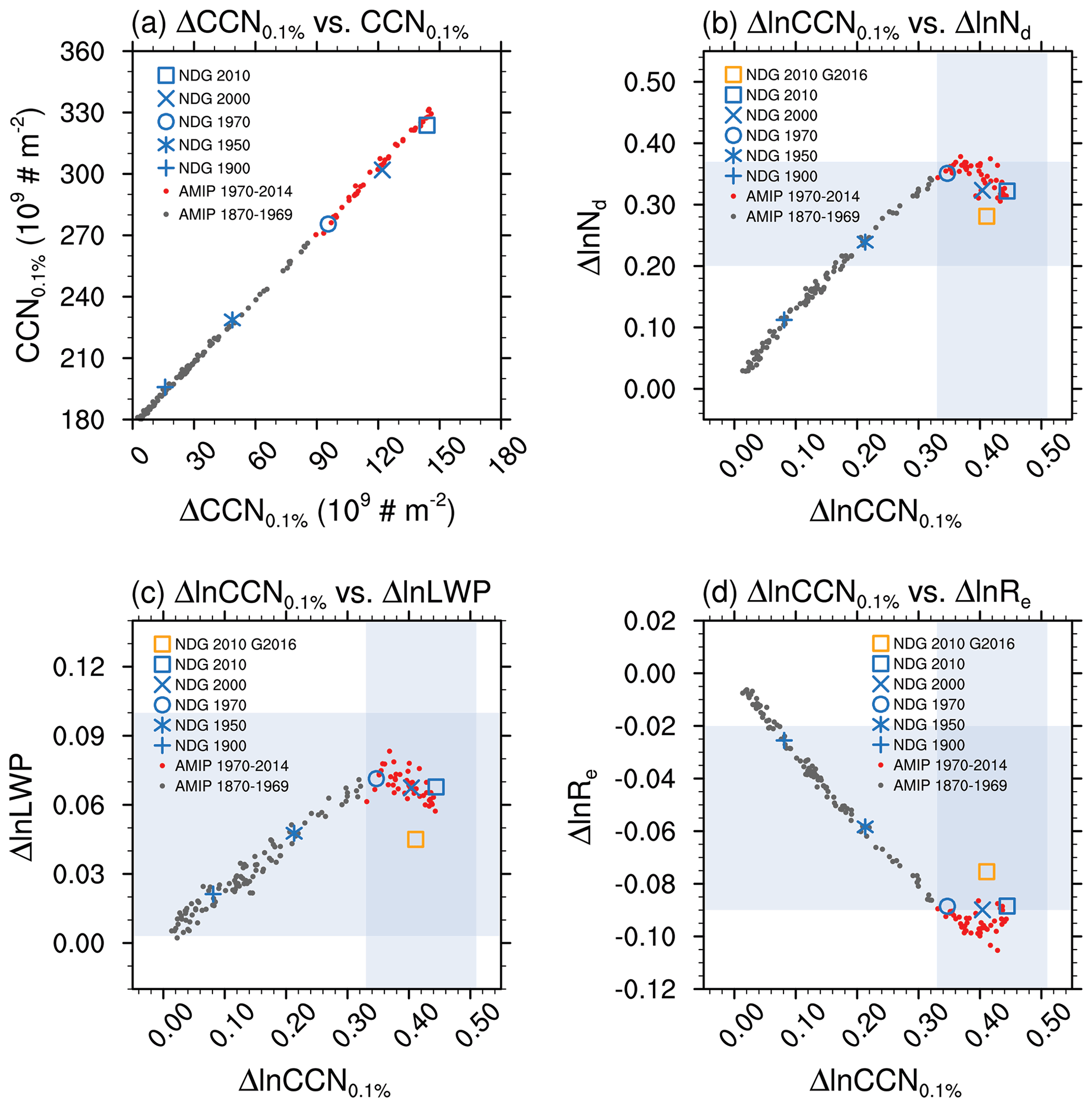
Figure 8As Fig. 7, but for relationships between the relative changes in CCN (ΔlnCCN0.1 %) and in liquid cloud properties including droplet number (ΔlnNd), liquid water path (ΔlnLWP), and effective radius of cloud droplets at cloud top (Δln Reliq). . Dark grey dots indicate estimated values from AMIP PD/PI simulations for the years 1870–1969, while red dots are the estimated values for the years 1970–2014. Each dot represents the ensemble-averaged global annual mean field for a certain year. Blue markers show the estimates based on nudged simulations. The orange square shows the nudged simulation results averaged from conditionally sampled high-frequency data following Ghan et al. (2016), wherein CCN (at 0.3 % supersaturation) and Nd are sampled below 1 km and at the top of liquid clouds. The grey area indicates the multi-model estimated range from Ghan et al. (2016). See Sect. 4.2 for details.
Figure 8 shows the relationships between simulated relative changes in column-integrated CCN at 0.1 % supersaturation (ΔlnCCN0.1 %) and in cloud microphysical quantities, including cloud droplet number concentration (ΔlnNd), liquid water path of stratiform clouds (ΔlnLWPstrat), and cloud-top droplet effective radius (ΔlnReliq). The global annual mean CCN0.1 % increases by more than 80 % from the pre-industrial era to present-day conditions. Compared to the year 1970, the global annual mean ΔCCN0.1 % increases by more than 60 % in the year 2010. However, it shows opposite trends in the NH polar region and in the tropics (see Figs. S1 and S3).
Before 1970, there is strong positive correlation between ΔlnNd and ΔlnCCN0.1 % (grey dots in Fig. 8b) and between ΔlnLWPstrat and ΔlnCCN0.1 % (Fig. 8c) but a negative correlation between Δln Reliq and ΔlnCCN0.1% (Fig. 8d). This is consistent with the causal relationship between these quantities simulated in the model (more CCN leads to higher Nd and LWP but smaller Reliq) and the fact that all types of anthropogenic aerosol emissions increase (so does CCN) from the pre-industrial era to about 1970 (see Fig. 1).
After 1970, the correlation between these global quantities become weaker (red dots in Fig. 8b–d). This is mainly caused by three factors. First, more primary (carbonaceous) aerosols and less secondary (sulfate) aerosols decrease the particle hygroscopicity and size, which subsequently reduce the droplet nucleation even if CCN0.1 % does not change much (e.g., Figs. S1b and S2b). The impact of carbonaceous aerosol increase is most evidently seen from the differences between 2000 and 2010 (Fig. 9a, b). ΔlnCCN0.1 % slightly increases in the NH polar and NH midlatitude regions, while ΔlnNd decreases in both regions.
Second, there are regional differences in the simulated relationships. The large regional differences in ΔlnNd and ΔlnCCN0.1 % contribute to the temporal variations of global mean values. In the NH polar region, CCN0.1 % increases before 1970 but decreases afterwards (Figs. 9a and S1a). In midlatitudes, CCN0.1% is stabilized after 1970 as a result of the increase in Asia and the decrease in North America. In the tropics, CCN0.1 % increases continuously during the whole simulation period (Figs. 9a and S3a). Consequently, there is an increase in the global mean ΔlnCCN0.1 %. In contrast, the global mean ΔlnNd is greatly affected by the decreases in both the NH polar and NH midlatitude regions, so it decreases slightly after 1970. Although ΔlnNd still increases continuously in the tropics, the value is much smaller than those in the NH polar and NH midlatitude regions.
Third, the CCN–Nd relationship also appears to have a “saturation effect” (Martin et al., 1994; Boucher and Lohmann, 1995; Stevens, 2015), which means a saturation in Nd with increasing aerosol number or CCN. The saturation effect can be caused by (1) reduced wet growth by carbonaceous aerosols (Martin et al., 1994), which has a similar effect as the first factor, and (2) a suppression in the maximum supersaturation (that the air parcel can have) caused by more CCN; this will lead to a reduced fraction of CCN that is activated (Chuang et al., 2000). As shown in Fig. 9c, the slope (ΔlnlnCCN0.1 %) calculated using regional mean fields slightly decreases from 1900 to 2010 for all the inspected regions.
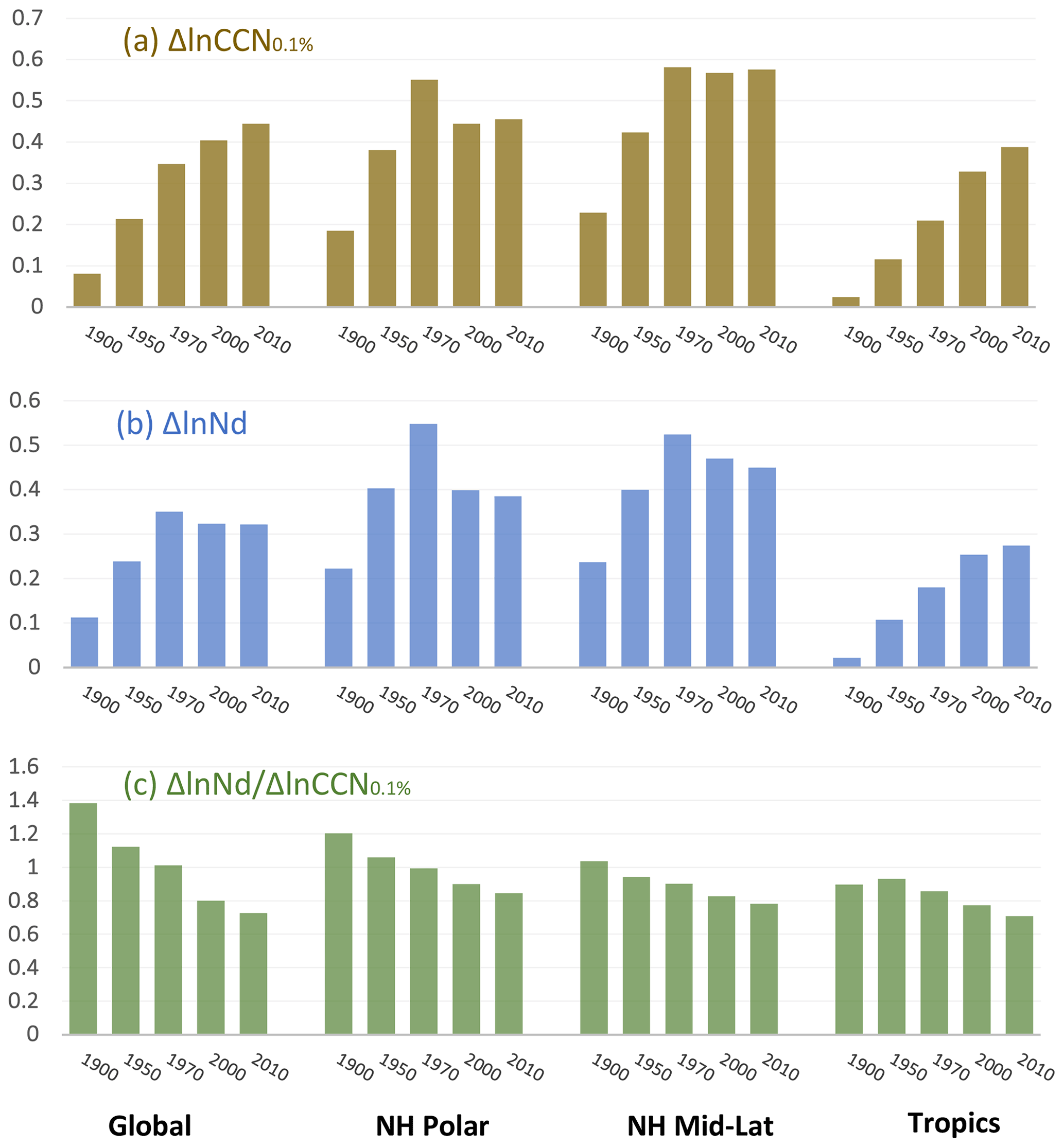
Figure 9Global and regional annual mean relative changes in CCN (ΔlnCCN0.1 %, a) and Nd (ΔlnNd, b) due to differences in anthropogenic aerosols between PI (1850) and PD (2010). Panel (c) shows the ratio between ΔlnNd) and ΔlnCCN0.1 %. See Sect. 4.2 for details.
Compared to the multi-model estimates reported in Ghan et al. (2016), the estimated values of ΔlnCCN0.1 %, Δln Nd, and ΔlnLWPstrat in E3SMv1 are all well within the min-to-max range (almost right in the middle). However, we find that the estimated Δln Reliq magnitude in E3SMv1 is relatively large compared to the multi-model estimates.
4.3 Susceptibility of Reliq, LWP, τliq, and cloud radiative forcing to changes in Nd
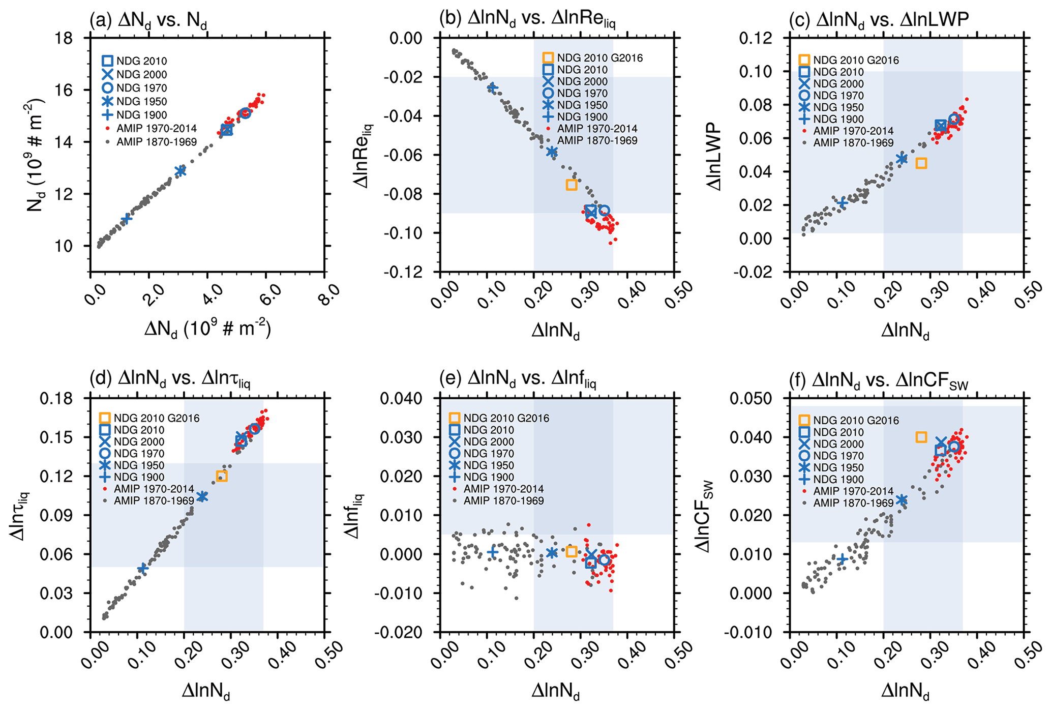
Figure 10As Fig. 7, but for relationships between ΔNd and Nd and between relative changes in Nd and other quantities. Δln τliq, Δln fliq, and ΔlnCFSW are the relative changes in liquid cloud optical depth, liquid cloud fraction, and shortwave cloud radiative forcing, respectively. . Dark grey dots indicate estimated values from AMIP PD/PI simulations for the years 1870–1969, while red dots are the estimated values for the years 1970–2014. Each dot represents the ensemble-averaged global annual mean field for a certain year. Blue markers show the estimates based on nudged simulations. The orange square shows the nudged simulation results averaged from conditionally sampled high-frequency data following Ghan et al. (2016), wherein CCN (at 0.3 % supersaturation) and Nd are sampled below 1 km and at the top of liquid clouds. The grey area indicates the multi-model estimated range from Ghan et al. (2016). See Sect. 4.3 for details.
Figure 10 shows the relationships between simulated relative changes in column-integrated Nd (Δln Nd) and in other cloud microphysical quantities, including cloud-top droplet effective radius (Δln Reliq), liquid and ice water path of stratiform clouds (ΔlnLWP and ΔlnIWP), cloud optical depth (Δln τliq), liquid cloud fraction (Δln fliq), and shortwave cloud radiative forcing (ΔlnCFSW). For the sampling using monthly model output, Δln Nd, ΔlnLWP, and ΔlnIWP (for stratiform clouds) are calculated using grid mean values. Δln Reliq and Δln τliq are calculated using in-cloud values, which are sampled using the COSP (Cloud Feedback Model Intercomparison Project Observation Simulator Package) simulator and derived during post-processing. For the sampling using high-frequency data (orange square in Figs. 7–10) following Ghan et al. (2016), they are in-cloud values calculated using the grid box mean values divided by the cloud cover after averaging in time and space. Because they are relative changes in global annual mean quantities, using in-cloud values (derived from grid mean values and cloud cover after averaging in time and space) or grid average values gives very similar results.
The global annual mean Nd increases by about 50 % from the pre-industrial era to present-day conditions (blue square in Fig. 10a). Compared to the year 1970, the global annual mean Nd is smaller in the year 2010, which is different from the results we see in τa (Fig. 7a) and CCN0.1 % (Fig. 8a). More aerosols simulated in the model (in terms of global annual mean) do not necessarily lead to an increase in Nd, since there are regional decreases in the sulfate burden that reduce the aerosol hygroscopicity and subsequent aerosol activation. On the other hand, similar opposite trends (as for ΔlnCCN0.1 %) appear in the NH polar region (decreases after 1970) and in the tropics (increase continuously after 1970).
There is a strong negative correlation between Δln Nd and Δln Reliq (grey and red dots in Fig. 10b). There is also strong positive correlation between Δln Nd and other quantities including ΔlnLWP, Δln τliq, and ΔlnCFSW (Fig. 10c, d, f). The results are consistent with the causal relationship between these quantities simulated in the model (more Nd leads to larger LWP but smaller Reliq). Unlike ΔlnCCN0.1 %, after 1970, the correlation between Nd and other global quantities is very similar to those before 1970. Since the relations shown in Fig. 10 characterize cloud properties (instead of the relations between aerosols and clouds), the lack of a change in slope (as in Fig. 8) is expected.
4.4 Relationships between changes in liquid and ice cloud properties
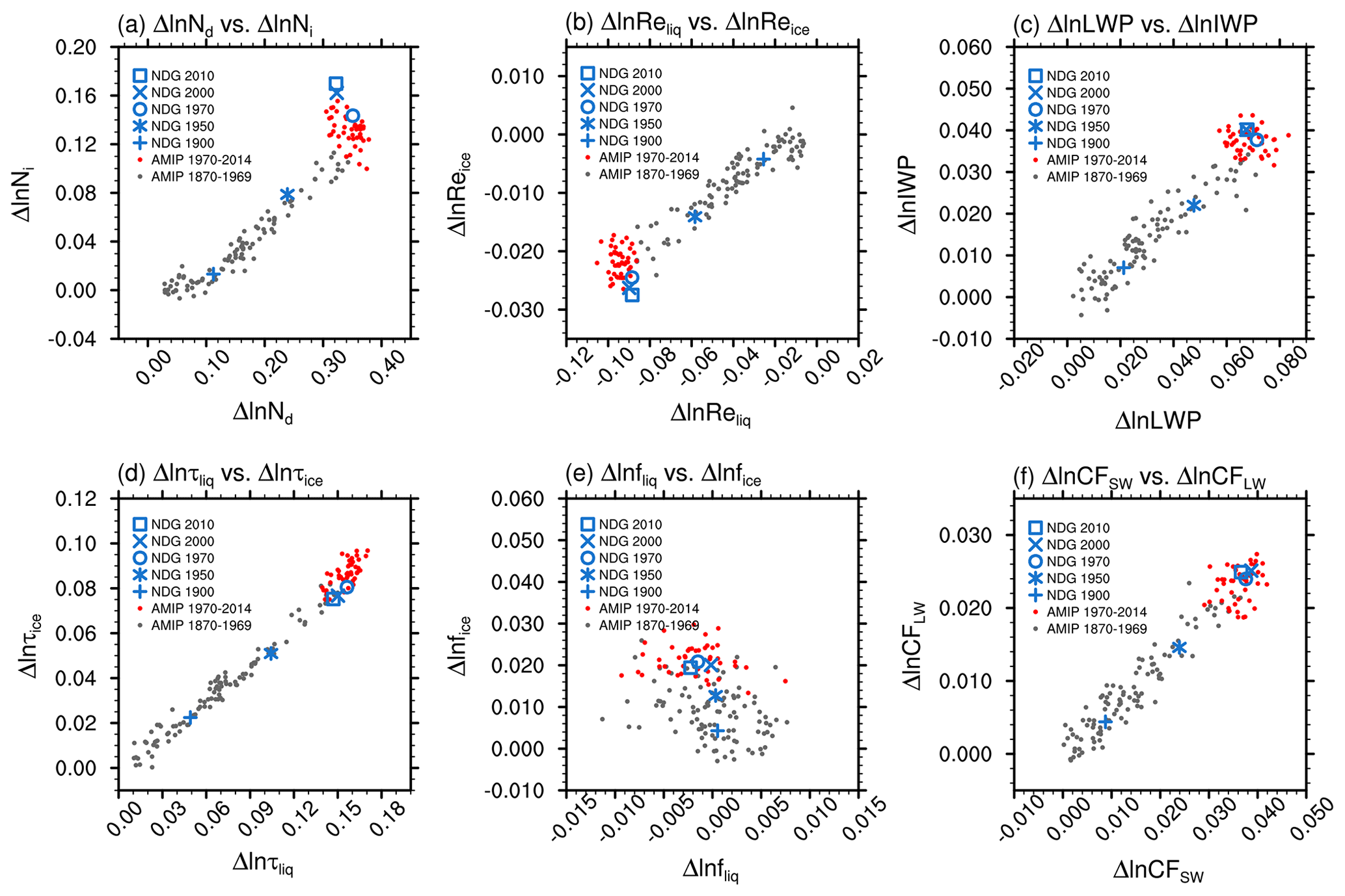
Figure 11As Fig. 7, but for relationships between changes in liquid and ice cloud properties as well as in SW and LW cloud radiative forcing. Δln Reice, ΔlnIWPice, Δln τice, Δlnfice, and ΔlnCFLW are the relative changes in the effective radius of cloud ice at the cloud top, ice water path in stratiform clouds, ice cloud optical depth, ice cloud fraction, and longwave cloud radiative forcing, respectively. . Dark grey dots indicate estimated values from AMIP PD/PI simulations for the years 1870–1969, while red dots are the estimated values for the years 1970–2014. Each dot represents the ensemble-averaged global annual mean field for a certain year. Blue markers show the estimates based on nudged simulations. See Sect. 4.4 for details.
As described in Sect. 2.1.2, E3SMv1 considers the activation of aerosol particles to cloud droplets and the freezing of cloud droplets to ice crystals in mixed-phase clouds when ice nuclei are available. It also considers the homogeneous ice nucleation of sulfate aerosols and heterogeneous ice nucleation of dust aerosols in cirrus clouds. Because dust is natural and the ice nucleation rate caused by BC is rather small (compared to the contribution by dust), sulfate is the dominant anthropogenic aerosol type that affects both the droplet (and the subsequent freezing) and ice crystal formation processes.
Figure 11 shows the relationships between simulated relative changes in liquid and ice cloud properties. There are strong positive correlations between the changes in the liquid and ice cloud quantities for the global annual mean column-integrated particle number (Δln Nd vs. Δln Ni), cloud-top effective radius (Δln Reliq vs. Δln Reice), column-integrated water path in stratiform clouds (ΔlnLWP vs. ΔlnIWP), and cloud optical depth (Δln τliq vs. Δln τice). The ice properties shown here do not consider the contribution from snow. On the other hand, the relative changes in liquid and ice cloud fractions are not well-correlated. Compared to liquid clouds, the ice cloud properties have a similar but slightly weaker sensitivity to changes in anthropogenic aerosols (Fig. S4).
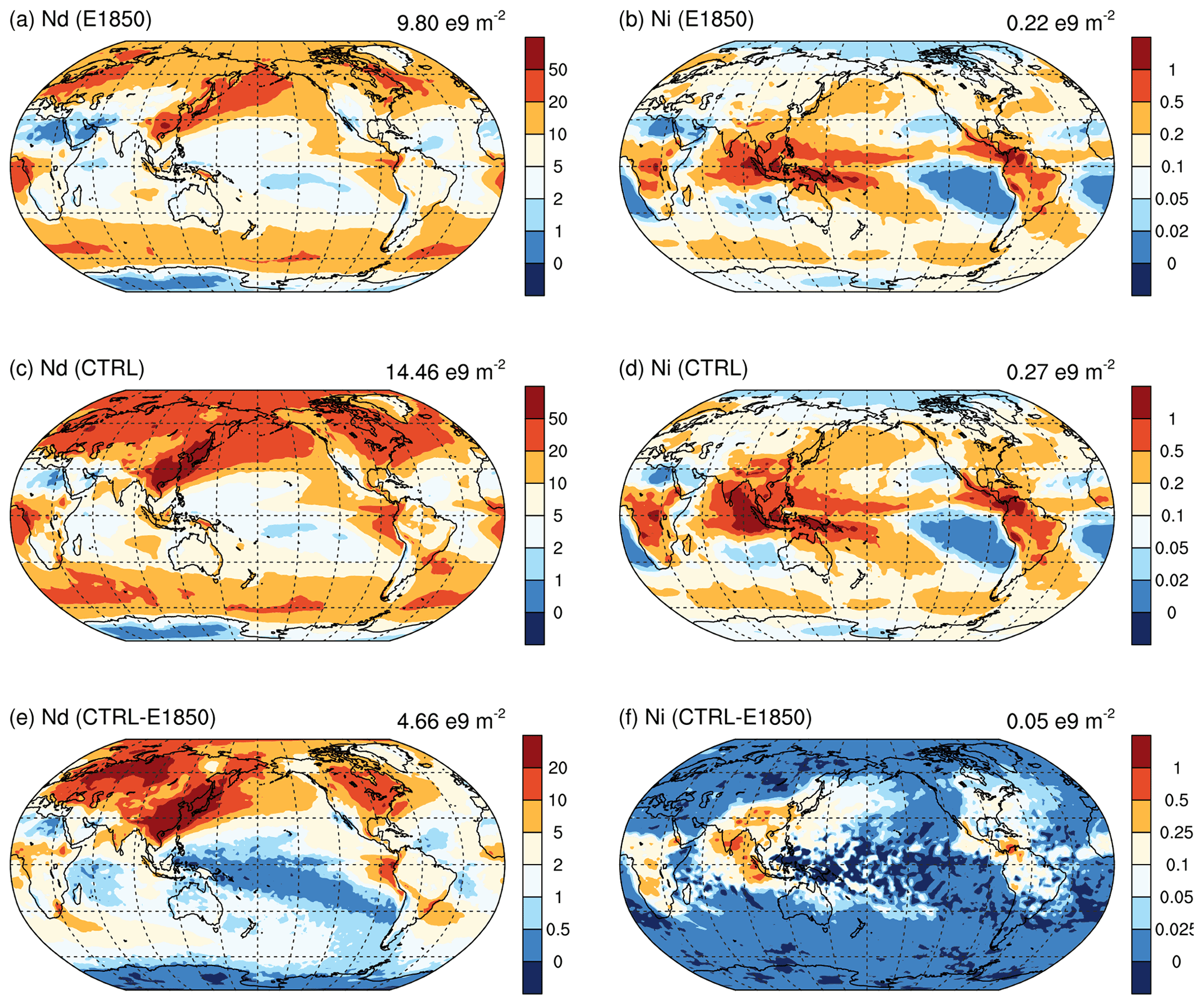
Figure 12Annual mean column-integrated cloud droplet and ice crystal number concentrations for the pre-industrial era (E1850, panels a, b), present day (CTRL for year 2010, panels c, d), and PD–PI differences (e, f) in the nudged simulations. See Sect. 4.4 for details.
The relative change in global annual mean column-integrated droplet number concentration (Δln Nd in Fig. 11a, also in Fig. 10) increases from the pre-industrial era but starts to decrease after 1970. This is not the case for the relative changes in the column-integrated ice crystal number, for which we see a continuous increase. This difference is mainly caused by the fact that the major changes in Nd and Ni appear in different regions. As shown in Fig. 12, the largest changes in Nd are in NH midlatitude and polar regions, where anthropogenic aerosols affect the low liquid cloud most. In contrast, the largest changes in Ni are mainly in the tropics and subtropics regions, where the cirrus clouds are affected by anthropogenic sulfate particles through homogeneous ice nucleation. In our model, the homogeneous ice nucleation in cirrus clouds is parameterized based on Liu et al. (2005) and Gettelman et al. (2010). We use the aerosol number concentration in the Aitken mode truncated at a specified cutoff diameter (50 nm in CTRL) to estimate the number of sulfate aerosol particles that can initiate homogeneous ice nucleation. Similar to findings in Gettelman et al. (2010), the parameterized homogeneous ice nucleation in E3SMv1 is sensitive to the sulfate aerosol number, and there is a large difference between PD and PI simulations (this is further discussed in Sect. 6). The anthropogenic aerosol effects on Ni below 300 hPa (mainly in mixed-phase clouds) are very small.
In this section, we decompose the effective aerosol forcing based on the method proposed by Ghan (2013) and based on the individual aerosol forcing and emission types. These decompositions help us understand the role of various forcing mechanisms and the impacts of individual aerosol compositions on the overall ERFaer.
5.1 Decomposition of ERFaer due to the aerosol–radiation interaction, aerosol–cloud interaction, and surface albedo effect

Figure 13Geographical distributions of decomposed net (left column), shortwave (middle column), and longwave (right column) ΔF at the top of the model (TOM). The decomposition calculation follows Ghan (2013). ALL indicates the total ΔF calculated from the difference between CTRL and E1850 (ALL = ARI + ACI + RES). ACI indicates the ΔF caused by aerosol–cloud interactions (second row), ARI the ΔF caused by aerosol–radiation interactions (third row), and RES (bottom row) the residual forcing. The clear-sky direct aerosol effect (fourth row) is also shown. See Sect. 5.1 for details.
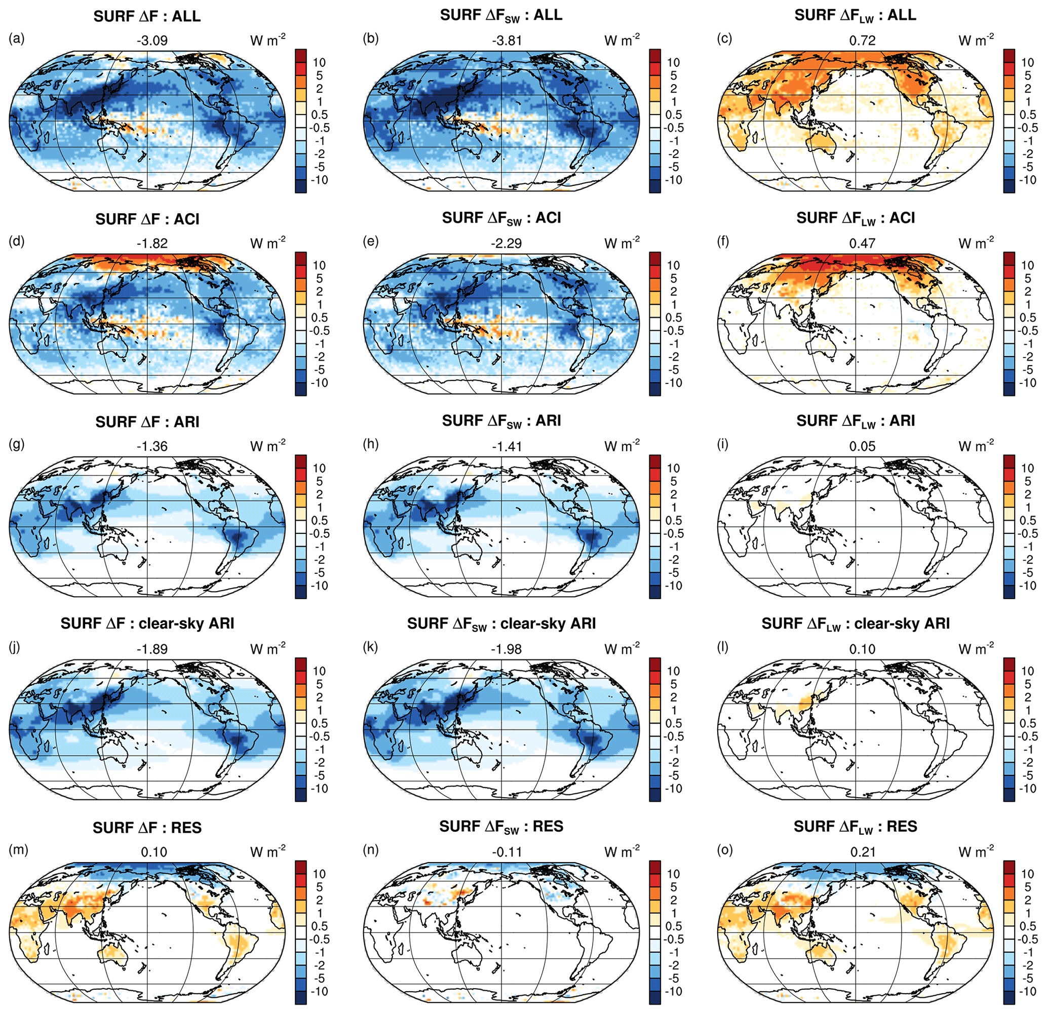
Figure 14Geographical distributions of decomposed net (left column), shortwave (middle column), and longwave (right column) ΔF at the surface. The decomposition calculation follows Ghan (2013). ALL indicates the total ΔF calculated from the difference between CTRL and E1850 (ALL = ARI + ACI + RES). ACI indicates the ΔF caused by aerosol–cloud interactions (second row), ARI the ΔF caused by aerosol–radiation interactions (third row), and RES (bottom row) the residual forcing. The clear-sky ARI (fourth row) is also shown. See Sect. 5.1 for details.
We use the Ghan (2013) method to decompose the total ERFaer (ΔF) into individual forcings caused by aerosol–radiation interactions (ARI, direct aerosol effect), aerosol–cloud interactions (ACI, mainly from indirect aerosol effect), and the residual term (mainly from surface albedo effect). To do this, an additional call to the radiation calculation is added in the model to calculate the radiative fluxes without considering the aerosol scattering and absorption of shortwave radiation in the calculation for all-sky (Fclean) and clear-sky (Fclear,clean) conditions.
The decomposed forcings are calculated as follows.
-
Aerosol–radiation interaction (“direct radiative forcing” in Ghan, 2013): Δ(F − Fclean)
-
Aerosol–cloud interaction (“cloud radiative forcing” in Ghan, 2013): Δ(Fclean− Fclear,clean)
-
Residual forcing (“surface albedo forcing” in Ghan, 2013): ΔFclear,clean
We note that F and Fclean are calculated in a single simulation. They both include the impact of ACI, which is considered the same for the two terms in the decomposition calculation. In addition to the indirect aerosol effect, the ACI term (“cloud radiative forcing” in Ghan, 2013) also includes the semi-direct aerosol effect (light-absorbing aerosols can heat the atmosphere and affect clouds), although the estimated effect is much smaller than the indirect aerosol effect (Ghan et al., 2012).
Figure 13 shows the geographical distributions of the decomposed top-of-model ΔF for the year 2010 using the nudged simulations with E3SMv1 (CTRL – E1850). The forcing caused by aerosol–cloud interactions has the largest contribution to the overall ΔF. In contrast, the global annual mean forcing caused by aerosol–radiative interactions is very small (0.04 W m−2), but it is positive over subtropical land and stratocumulus-prevalent regions, where BC absorption of shortwave radiation is strong (especially above clouds). The large positive forcing due to aerosol–radiative interactions off the Peruvian coast is mainly caused by absorption enhancement caused by the light-absorbing aerosols (mainly by biomass burning aerosols) above highly reflective clouds (Haywood and Shine, 1997). The clear-sky aerosol forcing is overall negative, except over North Africa and the Arabian Peninsula, where there are significant changes in absorbing aerosols. The residual forcing (ΔFclear,clean) is negative over the NH polar region, which is mainly caused by anthropogenic sulfate aerosols. Positive forcing appears over subtropical land areas and is caused by both shortwave (surface albedo effect) and longwave (water vapor) changes.
At the surface, the anthropogenic aerosol effect through the interactions with radiation contributes to more than 40 % of the total forcing (Fig. 14g). Large surface longwave ACI appears in the NH high-latitude and polar regions (Fig. 14f), which is caused by more low liquid cloud induced by anthropogenic aerosols. The thicker liquid clouds can trap more outgoing longwave radiation and emit it back to the surface. As discussed in Sect. 7, this causes a strong increase in the near-surface temperature during the boreal winter season.
5.2 Decomposition of forcing by individual compositions
To investigate the impact of changes in individual aerosol compositions, we decompose ΔF based on the different anthropogenic aerosol emission types that contribute to the total forcing. To do this, we change one type of aerosol emission in E1850 at a time from the pre-industrial condition to the 2010 level so that the contribution of this single emission type can be estimated. All other aerosol emissions are set to pre-industrial conditions. Note that we take the 1850 aerosol condition as the background. Due to the nonlinear effect (e.g., BC mixing state in 1850 is different from that in 2010), the sum of the estimated forcings by individual aerosol species would not be the same as the total forcing estimated using CTRL and E1850.
Figure 15 shows the geographical distributions of the decomposed ΔF for individual aerosol emission types. The anthropogenic sulfur emission has a large impact on the ΔF (Fig. 15d). The global annual mean net forcing is about −1.66 W m−2, which is very close to the ΔF estimate due to all aerosol emission changes. However, both the shortwave and longwave ΔF magnitudes increase significantly (by 0.25 W m−2), and they compensate for each other. The anthropogenic BC emission has an overall positive ΔF (Fig. 15g), with a global annual mean net forcing of 0.27 W m−2. The positive ΔF over land is mainly caused by the shortwave absorption of BC (Fig. 15h).
The compensating changes over the Tropical Warm Pool region (ΔFSW and ΔFLW) are mainly caused by reduced high clouds in that area. The impacts of the anthropogenic POM and SOA emissions on ΔF are overall negative (−0.3 to −0.4 W m−2, Fig. 15j, m). The impacts of biomass burning emission changes (BB) on ΔF are mostly in the shortwave, and they have a distinct regional pattern (Fig. 15m, n). Over Siberia, BB ΔF is positive (mainly in JJA and MAM), while over the west of Columbia, Ecuador, and Peru, there is a significant negative forcing (in JJA and SON). This suggests that there are large differences of BB emissions near (or on the upwind side) these two regions between the pre-industrial (1850) and present-day (2010) emissions.
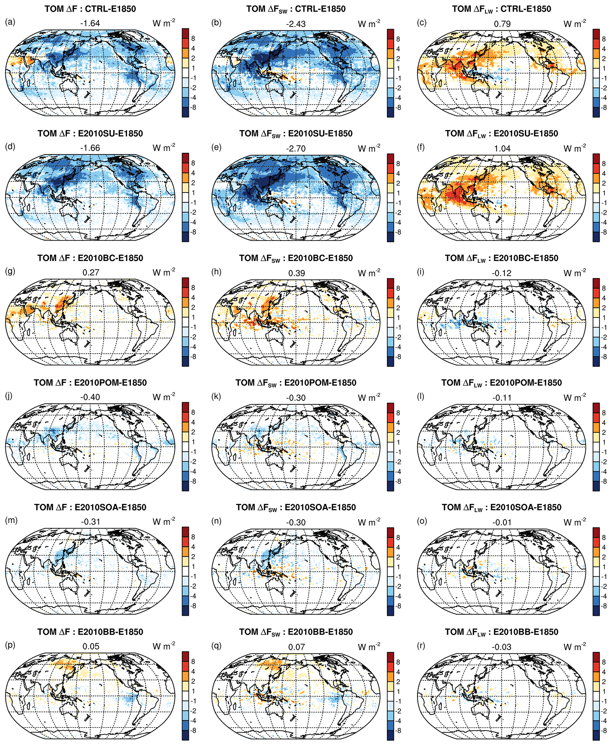
Figure 15Geographical distributions of the annual mean net (left column), shortwave (middle column), and longwave (right column) top-of-model (TOM) effective radiative forcing by individual aerosol components (i.e., compositions). For example, “E2010SU” indicates the same simulation as E1850 but with present-day (2010) sulfur emissions. See Sect. 5.2 and Table 1 for details.
Table 2Global and annual mean net, shortwave (SW), and longwave (LW) ERFaer (W m−2) at the top of the model (TOM) and surface in the nudged simulations. Model configurations are described in Table 1.

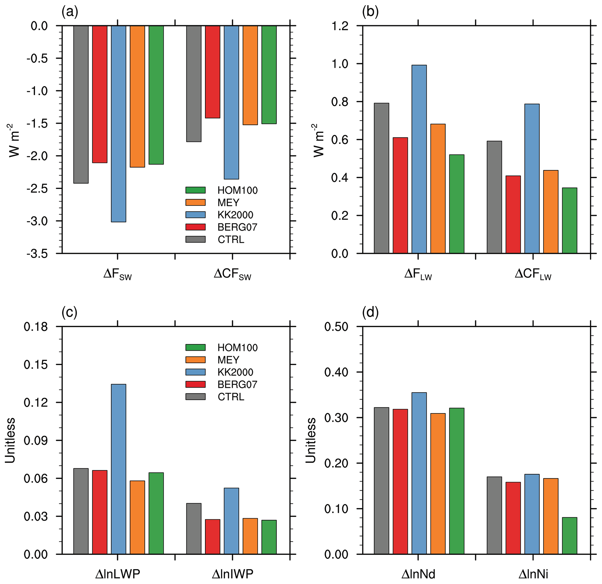
Figure 16Global annual mean anthropogenic aerosol effects on top-of-model (TOM) radiative fluxes (ΔF and ΔCF) and hydrometeor mass and number (relative changes) in the reference and sensitivity simulations. CFSW and CFLW are shortwave and longwave cloud radiative forcings. LWP and IWP are the liquid and ice water path in stratiform clouds. Nd and Ni are the column-integrated droplet and ice number concentrations. . See Sect. 6 for details.
Based on the sensitivity simulations performed during the model development, we have identified several parameterization changes that have important impacts on the anthropogenic aerosol effect in the model. These include changes in cloud microphysics that affect the autoconversion in warm clouds, the Bergeron process and heterogeneous ice nucleation in mixed-phase clouds, and homogeneous ice nucleation in cirrus clouds (see Table 1).
As described in Rasch et al. (2019), E3SMv1 uses a modified autoconversion scheme based on Khairoutdinov and Kogan (2000) (hereafter KK2000), wherein the parameters have been tuned so that the autoconversion process converts less liquid to rain compared to the standard KK2000 treatment. As a result, the liquid water content increases less rapidly (especially under more pristine conditions) when the aerosol and cloud droplet number concentrations are small. With the parameters reset to KK2000 standard values, the liquid water path is decreased significantly in most regions (Fig. S6e). In contrast, the changes in liquid water path between the PD and PI simulations become larger (Figs. 16c and S6f). Consequently, the simulated anthropogenic aerosol effect (−2.03W m−2) is much larger than the reference model (Table 2 and Fig. 16).
The Bergeron process rate determines how much liquid is converted to ice through the Wegener–Bergeron–Findeisen process. In E3SMv1, a scaling factor was set to make the Bergeron process rate 10 % of its nominal value. This was originally intended to compensate for an overestimated ice formation rate when using the Meyers scheme (Meyers et al., 1992). The overly small Bergeron process rate produces too much supercooled liquid cloud in the simulation. By changing the scaling factor from 0.1 to 0.7, the liquid and ice water path is decreased in most places, especially in midlatitude and polar regions (Figs. S6c and S7c). The changes in liquid and ice water paths between the PD and PI simulations also become smaller (Figs. S6d and S7d). As a result, the simulated anthropogenic aerosol effect is significantly weaker than the reference model for both the shortwave and longwave components (Table 2 and Fig. 16).
E3SMv1 uses the CNT-based heterogeneous ice nucleation scheme to consider the ice formation in mixed-phase clouds (Wang et al., 2014). Compared to the Meyers scheme (Meyers et al., 1992) used in E3SMv0, the CNT scheme predicts less heterogeneous ice nucleation and freezes less supercooled liquid (Figs. 16c and S6h), especially in the NH polar region. The increased supercooled liquid amount leads to optically thick liquid clouds in the lower troposphere, which subsequently increase the downward longwave radiation and warm the surface in the NH polar region (this is further explained in the next section). A much larger impact has been seen in the high-resolution simulations (Caldwell et al., 2019), which reported severely overestimated Arctic surface temperature when the CNT scheme was used along with the 0.1 Bergeron process rate scaling factor. This might be related to the fact that the high-resolution model can better resolve the heterogeneity in cloud phase (Tan and Storelvmo, 2016). As mentioned in Caldwell et al. (2019) and above, it is more reasonable to use a larger scaling factor (e.g., 0.7 instead of 0.1) when the parameterization uses the CNT scheme. When the Meyers scheme is used, the relative changes in the column-integrated mass and number are reduced for both cloud liquid and ice, leading to a reduced ERFaer in both the shortwave and longwave components. Similar sensitivities were found in the CAM6/CESM2 model simulations (Gettelman et al., 2019).
In E3SMv1, the threshold size of Aitken sulfate aerosols for homogeneous ice nucleation was adjusted to 50 nm in the DECK simulation setup from the original 100 nm value used in CAM5. This allows more Aitken-mode sulfate particles to nucleate ice homogeneously, which greatly increases the ice crystal number concentration and their subsequent growth. When the threshold size is reset to 100 nm, the ice crystal number and ice water content decrease by about a factor of 2 in most regions (Fig. S7i), and the changes in ice crystal number and ice water content between the PD and PI simulations become smaller (Figs. 16d and S7j). As a result, the simulated anthropogenic aerosol effects in both the shortwave and longwave are reduced compared to the reference model (Table 2). Due to the strong compensation between the changes in SW and LW, the change in the net effect is fairly small (−1.62 vs. −1.64 Wm−2 in the reference model).
We note that the sensitivities discussed above are likely dependent on the quantity of simulated background (pre-industrial) aerosols and cloud hydrometeor concentrations in the model. For example, the autoconversion rates estimated by the original and modified KK2000 parameterizations depend on the droplet number concentrations, and the difference between them is large under pristine conditions (in which the cloud droplet number is small, see Fig. 2 in Rasch et al., 2019).
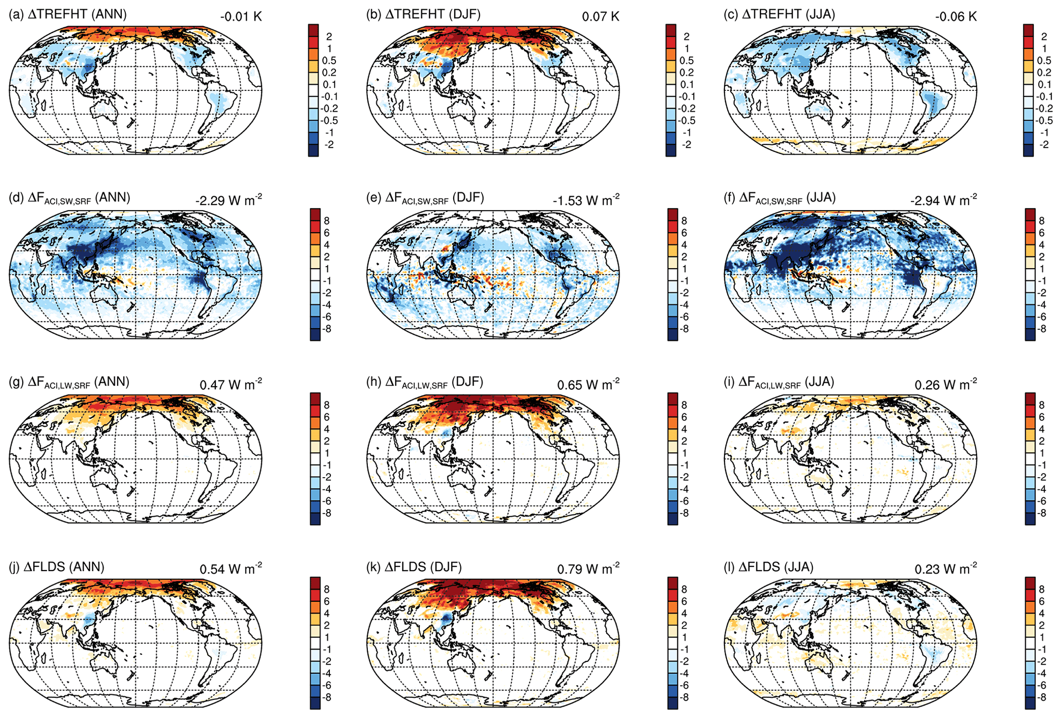
Figure 17Global annual and seasonal mean changes in near-surface temperature at 2 m (ΔTREFHT, K), decomposed ACI forcing at the surface (ΔFACI,SRF, W m−2), and downward longwave radiation flux (ΔFLDS, W m−2) due to the anthropogenic aerosol effects. See Sect. 7 for details.
The near-surface temperature is strongly affected by the radiative heating and cooling caused directly or indirectly by anthropogenic aerosols through fast processes. The “fast processes” defined here are processes that do not involve the ocean feedback to the atmosphere (in response to the anthropogenic aerosol forcing). Our definition of “fast processes” is slightly different from the “rapid adjustment” by Sherwood et al. (2015), which means “changes that occur directly due to the forcing, without mediation by the global-mean temperature”. As pointed out by Sherwood et al. (2015), the rapid adjustment may include fast changes in SST patterns caused by SST changes in areas with relatively shallow mixed layers. In this case, the global mean temperature change is negligible, but these SST changes can significantly affect the cloud and circulation patterns. Such rapid adjustments are not considered to be fast processes for our case.
Since the sea surface temperature is prescribed in our AMIP and nudged simulations, the impact of anthropogenic aerosols on sea surface temperature and the associated slow processes, such as the ocean circulation and its feedback to atmosphere, cannot be considered. Nevertheless, it is useful to estimate the impact of anthropogenic aerosols on the surface temperature through fast processes. The impact through slow processes can be inferred if both the AMIP and coupled simulation results are available.
We first look at the results from the nudged simulations. Since the large-scale circulation and SST are constrained, the local changes in diabatic heating and cooling (affected mainly by fast processes) have a dominant influence on the near-surface temperature over land. Fig. 17 (first row) shows the near-surface temperature (at 2 m) changes (ΔTREFHT) caused by the emission changes between pre-industrial and present-day conditions. As expected, near the emission sources and the downwind regions (especially in NH midlatitudes), anthropogenic aerosols in general have strong cooling effects. However, over the NH polar region, we see warmer surface temperature associated with responses over sea ice from increased anthropogenic aerosol emissions.
The increase in near-surface temperature mainly happens in the boreal winter season (Fig. 17b) and in late autumn and early spring, when the shortwave radiation is weak (due to the large solar zenith angle) and the longwave radiation plays a more important role in determining the near-surface temperature. Between simulations using 2010 and 1850 emissions, there is about a 0.5–2 K increase in December–January–February mean near-surface temperature over land and areas covered by sea ice near the Arctic. During the boreal summer season, the shortwave cooling effect is usually stronger than the longwave warming effect. Also, during the summer season the sea ice cover is smaller than in winter, and the near-surface temperature is less affected by the surface radiation changes. Therefore, the overall effect is cooling over land areas in the NH polar region (Fig. 17c), and over the Arctic Ocean the near-surface temperature change is not large.
In order to determine what processes cause the temperature increase in the NH polar region, we compared the seasonal mean near-surface temperature changes with the decomposed surface anthropogenic aerosol forcing (see previous section). The interaction between anthropogenic aerosols and clouds (ACI) has a strong warming effect at the surface (Fig. 17g, h). Furthermore, both the spatial pattern and the seasonal variations agree well with temperature increase. The strong ACI forcing is mainly contributed by the large increase in liquid water path (not shown). The thicker liquid clouds trap more outgoing longwave radiation and reflect it back to the surface (ΔFLDS in Fig. 17j, k), which causes the strong temperature increase in the boreal winter season. The results are consistent with previous observational studies (Garrett and Zhao, 2006; Lubin and Vogelmann, 2006), which reported a significant anthropogenic aerosol effect in the longwave over the Arctic through aerosol–cloud interactions.
Results from the AMIP simulations (Fig. 18) show a similar relationship between the changes in near-surface temperature and in the downward longwave radiation due to the anthropogenic aerosol effects. Note that we do not have the decomposed radiative forcing diagnostics output for the AMIP simulation, so here only the relationship between ΔTREFHT and ΔFLDS is shown. There is a strong correlation between ΔTREFHT and ΔFLDS time series. The temporal variations in ΔTREFHT and ΔFLDS are mainly affected by the interannual variations in both the liquid cloud distributions and the amount of anthropogenic aerosol. The nudged simulations (shown as dots) capture the changes in both variables well. This suggests that results from the relatively short nudged simulations can provide a reasonable estimate of the simulated near-surface temperature responses due to the anthropogenic aerosol forcing through the fast processes.
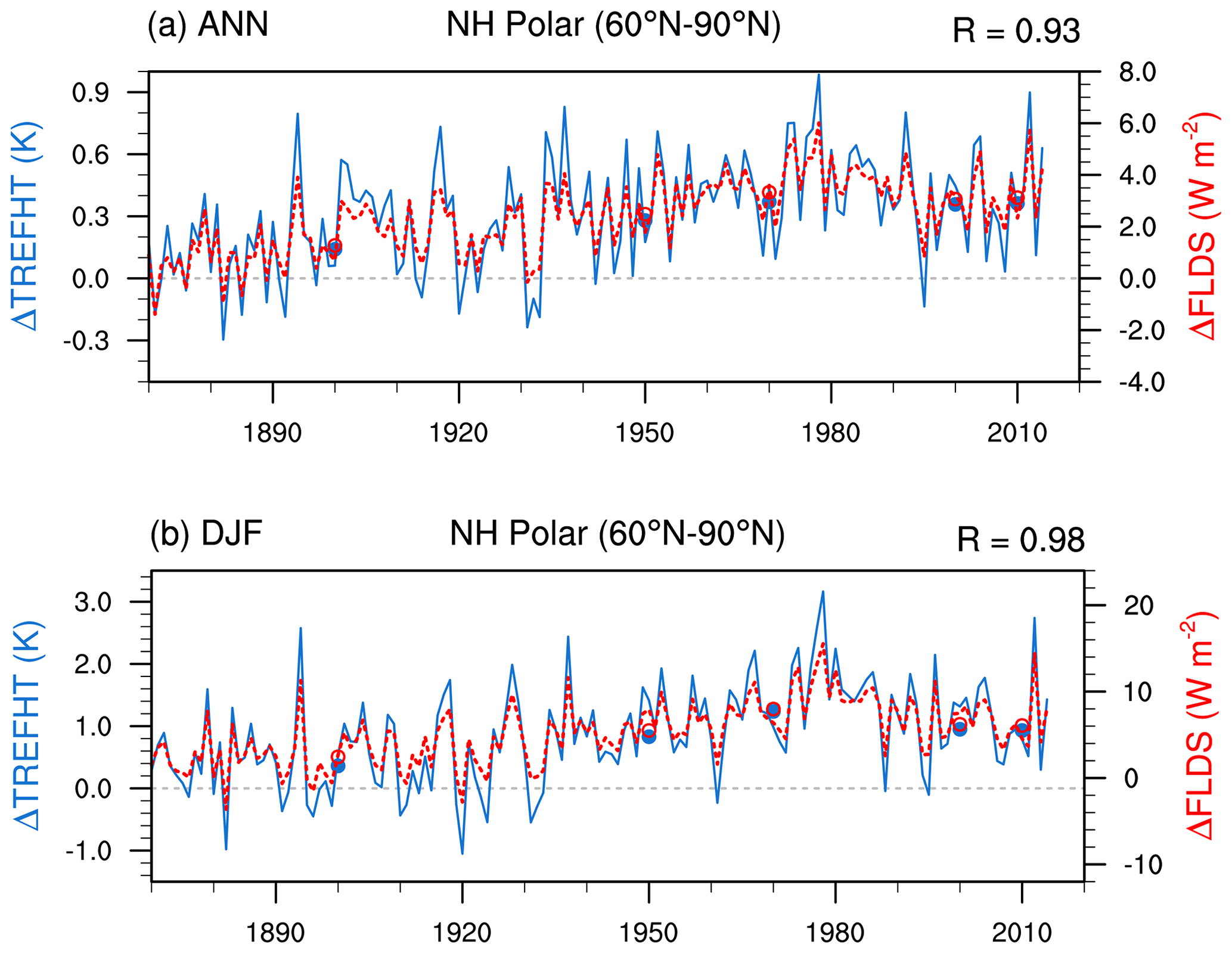
Figure 18Annual (a) and boreal winter (b) mean changes in near-surface temperature at 2 m (ΔTREFHT, K, in blue) and downward longwave radiation flux (ΔFLDS, W m−2, in red) over the NH polar region due to the anthropogenic aerosol effects. Both the AMIP (lines) and nudged (dots and circles) simulations are shown here. See Sect. 7 for details.
This study investigates the historical and present-day ERFaer in E3SMv1 using AMIP simulations for 1870–2014 and short nudged simulations. We analyze the relationship between key aerosol and cloud quantities, decompose the anthropogenic aerosol forcing in different ways, and evaluate the parameterization sensitivities.
Despite the overall increase in the global mean anthropogenic aerosol burden and optical depth (Δτa) during 1870–2014, there are large differences in the historical changes in these quantities between different regions and aerosol species. For example, the anthropogenic sulfate burden and sulfate Δτa over the NH polar regions and the NH midlatitude regions decrease significantly after 1970, while for carbonaceous aerosols, there is a continued overall increase in burden and Δτa. Both the shortwave and longwave ERFaer estimated by E3SMv1 are outside the 2 standard deviation range of the CMIP6 RFMIP model estimates (Smith et al., 2020), although they are not the strongest among the CMIP6 RFMIP model results. Similar to the changes in anthropogenic aerosol burden and optical depth, we see large regional differences in the temporal evolution of ERFaer. The overall increasing or decreasing trend in ERFaer resembles the changes in sulfate Δburden and Δτa, especially for NH midlatitude and polar regions.
The relative changes (dlnY versus dlnX) in historical global annual mean anthropogenic aerosol optical depths, CCN concentrations, and cloud droplet number concentrations show overall linear correlation. However, after around 1970, the correlations show a significant change. This is mainly caused by (1) the regional differences in the historical changes in anthropogenic aerosol burden and optical depths, as well as their impacts on the CCN and cloud droplet formation; (2) a shift from sulfate to carbonaceous aerosols in the anthropogenic aerosol composition; and (3) the “saturation effect”, as the slope slightly decreases from 1900 to 2010 for all the inspected regions. For ice cloud properties, we find similar but weaker correlations compared to those seen in liquid cloud properties.
A forcing decomposition analysis following Ghan (2013) shows that the top-of-model ERFaer in EAMv1 is dominated by the anthropogenic aerosol effect through the interactions with clouds. There is a strong compensation between the forcings in the shortwave and longwave components. At the surface, the anthropogenic aerosol effect through the interactions with radiation contributes to more than 40 % of the total forcing. Large surface longwave ACI forcing appears in the NH high-latitude and polar regions, which is caused by the increase in low liquid cloud induced by anthropogenic aerosols. The forcing analysis decomposed by aerosol species shows that anthropogenic sulfate aerosols have the largest effect (both in the shortwave and longwave) on the overall ERFaer. Anthropogenic BC aerosols exert a strong positive shortwave forcing due to absorption but a weaker negative longwave forcing by weakening vertical motions and reducing high cloud amounts. Both anthropogenic POM and SOA have significant negative forcing, but the forcing over the NH high-latitude and polar region is small.
We have also evaluated the sensitivity of simulated ERFaer to parameterization changes in EAM. Out of the four changes that were adopted in EAMv1, resetting the autoconversion tuning parameters (to the original values used in KK2000) has the largest impact on the net forcing (more negative), confirming that the autoconversion tuning parameters applied in EAMv1 indeed help to reduce the effective aerosol forcing. Two changes are made for mixed-phase clouds, i.e., the tuning of the Bergeron process rate and the change in ice nucleation scheme. Both of them significantly reduce the ERFaer in the shortwave and longwave components, but the impacts on the net forcing are relatively small. The last change, in homogeneous ice nucleation, makes the ice formation rate smaller in cirrus clouds. This also significantly reduces the aerosol forcing in both shortwave and longwave components, but the impact on net forcing is negligible.
The results summarized above suggest that in order to constrain the net ERFaer in future versions of E3SM, it is important to constrain the relative changes () in cloud droplet number concentrations (Nd) and liquid water path (LWP). In E3SMv1, very small Nd (e.g., Nd<10 cm−3) appears frequently under pristine conditions (to be presented in detail in a separate study). Applying a lower bound of cloud droplet number concentration can effectively increase Nd under pristine conditions and reduce Δln Nd in some models, though this treatment is artificial and thus not desirable (Hoose et al., 2009). One possible solution to reduce Δln Nd in a more physical way is to improve the representation of natural aerosols (especially for sulfate oxidized from DMS) and the associated cloud droplet formation or depletion processes in the model. Previous modeling studies have shown that the simulated aerosol radiative forcing is sensitive to DMS emission (Carslaw et al., 2013) and oxidation (Fung et al., 2022) treatments. The other way is to improve the droplet formation parameterization so that it can include some important processes (e.g., enhanced mixing induced by cloud-top radiative cooling, droplet spectral dispersion). These processes can usually only be resolved in model simulations at very high resolution (e.g., Zhang et al., 2022). How to parameterize them accurately in global models will be a challenge, and substantial changes might be needed for models like E3SM. Finally, as suggested by the sensitivity simulations, increasing the primary and/or secondary ice formation in mixed-phase clouds could also indirectly reduce Δln Nd and ΔlnLWP.
There are still some missing components or processes in our model. For example, the atmospheric chemistry is underrepresented in E3SMv1, wherein we only consider simple sulfur chemistry and the oxidants are prescribed. Related to this simplified treatment, nitrate aerosols are currently not treated in E3SMv1. Previous studies (e.g., Bellouin et al., 2011) have shown that nitrate aerosols have partly replaced sulfate in some regions (e.g., Europe). The overall effective aerosol forcing could maintain negative values in the future, even through some fossil fuel emissions are expected to continuously decrease. The representation of nitrate aerosols has been developed for a newer version of E3SM (Wu et al., 2022), with similar treatment used in CAM5 (Zaveri et al., 2021) and CAM6 (Lu et al., 2021). It would be interesting to investigate the impact of nitrate aerosols on the historical and future ERFaer changes using the new model.
In response to the aerosol forcing associated with fast processes (in contrast to the slow processes involving ocean and/or sea ice changes), significant regional changes are seen in the simulated near-surface air temperature. Due to the strong shortwave anthropogenic aerosol effect through ARI and ACI, surface cooling occurs in the midlatitude and low-latitude regions. Strong surface warming is seen in the NH high-latitude regions during boreal winter, which is mainly caused by denser liquid clouds in these regions that have a large impact on the longwave radiation. Since the warming caused by greenhouse gases is stronger over the polar regions than in lower latitudes, the high-latitude warming as well as midlatitude and low-latitude cooling caused by anthropogenic aerosols further amplify the meridional gradient in the near-surface temperature changes. The small change (close to zero) in the global mean surface temperature in the AMIP and nudged simulations suggests that the surface cooling in the second half of the 20th century simulated by the coupled model is very likely caused by the anthropogenic aerosol effects through slow processes involving ocean–sea ice responses. In the future, we plan to use both the AMIP and coupled simulations to further investigate the anthropogenic aerosol effects on the historical surface temperature change through different processes.
The model results presented in this study and the EAMv1/E3SMv1 source code can be found on Zenodo (https://doi.org/10.5281/zenodo.5792600, Zhang, 2021, and https://doi.org/10.5281/zenodo.5794575, E3SM developers, 2021). The EAMv1/E3SMv1 source code can also be found at https://github.com/E3SM-Project/E3SM/tree/v1.0.0 (last access: 10 July 2022; E3SM developers, 2021) (hash 849d9ee).
The supplement related to this article is available online at: https://doi.org/10.5194/acp-22-9129-2022-supplement.
KZ designed the study, performed (nudged) simulations and analyses, and wrote the first draft of paper. WZ contributed to the historical change analysis. HWan contributed to the simulation design and the causality analysis. SJG and MW contributed to the causality and decomposition analysis. PJR, PM, XS, YW, and XL contributed to the configuration and/or interpretation of sensitivity simulations. RCE, HWang, KZ, PM, SZ, JS, SB, MS, BS, YQ, YF, JHY, SJG, and PJR contributed to the aerosol–cloud model and analysis tool development. JCG, QT, WL, and SX contributed to the configuration and/or simulation of the AMIP runs. All authors contributed to the result discussion and paper revisions.
At least one of the (co-)authors is a member of the editorial board of Atmospheric Chemistry and Physics. The peer-review process was guided by an independent editor, and the authors also have no other competing interests to declare.
Publisher's note: Copernicus Publications remains neutral with regard to jurisdictional claims in published maps and institutional affiliations.
We thank the two anonymous reviewers for the helpful comments. This research was supported as part of the Energy Exascale Earth System Model (E3SM) project (grant no. 65814), funded by the US Department of Energy, Office of Science, Office of Biological and Environmental Research. We thank all E3SM team members for their efforts in developing and supporting the E3SM model. The Pacific Northwest National Laboratory (PNNL) is operated for the DOE by the Battelle Memorial Institute under contract DE-AC06-76RLO 1830. Wentao Zhang was partly supported by the Visiting Researchers (formerly Alternate Sponsored Fellow) Program at PNNL. Yan Feng would like to acknowledge the support of Argonne National Laboratory (ANL) provided by the US DOE Office of Science under contract no. DE-AC02-06CH11357. Work at LLNL was performed under the auspices of the US DOE by Lawrence Livermore National Laboratory under contract no. DE-AC52-07NA27344. Jin-Ho Yoon was supported by the National Research Foundation of Korea under NRF-2020M1A5A1110578 and NRF-2021R1A2C1011827. Manish Shrivastava acknowledges support through the DOE Biological and Environmental Research (BER) Early Career Research Program. This research used high-performance computing resources from the PNNL Research Computing and the National Energy Research Scientific Computing Center (NERSC), a DOE Office of Science User Facility supported by the Office of Science of the US Department of Energy under contract no. DE-AC02-05CH11231.
This research has been supported by the US Department of Energy (grant no. 65814).
This paper was edited by Hang Su and reviewed by two anonymous referees.
Abdul-Razzak, H. and Ghan, S. J.: A parameterization of aerosol activation – 2. multiple aerosol types, J. Geophys. Res., 105, 6837–6844, https://doi.org/10.1029/1999JD901161, 2000. a
Baró, R., Lorente-Plazas, R., Montávez, J. P., and Jiménez-Guerrero, P.: Biomass burning aerosol impact on surface winds during the 2010 Russian heat wave, Geophys. Res. Lett., 44, 1088–1094, https://doi.org/10.1002/2016GL071484, 2017. a
Bellouin, N., Rae, J., Jones, A., Johnson, C., Haywood, J., and Boucher, O.: Aerosol forcing in the Climate Model Intercomparison Project (CMIP5) simulations by HadGEM2-ES and the role of ammonium nitrate, J. Geophys. Res.-Atmos., 116, D20206, https://doi.org/10.1029/2011JD016074, 2011. a
Bellouin, N., Quaas, J., Gryspeerdt, E., Kinne, S., Stier, P., Watson-Parris, D., Boucher, O., Carslaw, K. S., Christensen, M., Daniau, A.-L., Dufresne, J.-L., Feingold, G., Fiedler, S., Forster, P., Gettelman, A., Haywood, J. M., Lohmann, U., Malavelle, F., Mauritsen, T., McCoy, D. T., Myhre, G., Mülmenstädt, J., Neubauer, D., Possner, A., Rugenstein, M., Sato, Y., Schulz, M., Schwartz, S. E., Sourdeval, O., Storelvmo, T., Toll, V., Winker, D., and Stevens, B.: Bounding Global Aerosol Radiative Forcing of Climate Change, Rev. Geophys., 58, e2019RG000660, https://doi.org/10.1029/2019RG000660, 2020. a, b, c, d, e, f, g, h, i, j
Bond, T. C. and Bergstrom, R. W.: Light Absorption by Carbonaceous Particles: An Investigative Review, Aerosol Sci. Technol., 40, 27–67, https://doi.org/10.1080/02786820500421521, 2006. a
Boucher, O. and Lohmann, U.: The sulfate-CCN-cloud albedo effect, Tellus B Chem. Phys. Meteorol., 47, 281–300, https://doi.org/10.3402/tellusb.v47i3.16048, 1995. a
Boucher, O., Randall, D., Artaxo, P., Bretherton, C., Feingold, G., Forster, P., Kerminen, V.-M., Kondo, Y., Liao, H., Lohmann, U., Rasch, P., Satheesh, S. K., Sherwood, S., Stevens, B., and Zhang, X. Y.: Clouds and aerosols, in: Climate change 2013: the physical science basis. Contribution of Working Group I to the Fifth Assessment Report of the Intergovernmental Panel on Climate Change, 571–657, Cambridge University Press, https://doi.org/10.1017/CBO9781107415324.016, 2013. a
Burrows, S. M., Easter, R. C., Liu, X., Ma, P.-L., Wang, H., Elliott, S. M., Singh, B., Zhang, K., and Rasch, P. J.: OCEANFILMS (Organic Compounds from Ecosystems to Aerosols: Natural Films and Interfaces via Langmuir Molecular Surfactants) sea spray organic aerosol emissions – implementation in a global climate model and impacts on clouds, Atmos. Chem. Phys., 22, 5223–5251, https://doi.org/10.5194/acp-22-5223-2022, 2022. a, b
Caldwell, P. M., Mametjanov, A., Tang, Q., Van Roekel, L. P., Golaz, J.-C., Lin, W., Bader, D. C., Keen, N. D., Feng, Y., Jacob, R., Maltrud, M. E., Roberts, A. F., Taylor, M. A., Veneziani, M., Wang, H., Wolfe, J. D., Balaguru, K., Cameron-Smith, P., Dong, L., Klein, S. A., Leung, L. R., Li, H.-Y., Li, Q., Liu, X., Neale, R. B., Pinheiro, M., Qian, Y., Ullrich, P. A., Xie, S., Yang, Y., Zhang, Y., Zhang, K., and Zhou, T.: The DOE E3SM Coupled Model Version 1: Description and Results at High Resolution, J. Adv. Model. Earth Syst., 11, 4095–4146, https://doi.org/10.1029/2019MS001870, 2019. a, b
Carslaw, K., Lee, L., Reddington, C., Pringle, K., Rap, A., Forster, P., Mann, G., Spracklen, D., Woodhouse, M., Regayre, L., and Pierce, J.: Large contribution of natural aerosols to uncertainty in indirect forcing, Nature, 503, 67–71, 2013. a, b
Chuang, P. Y., Collins, D. R., Pawlowska, H., Snider, J. R., Jonsson, H. H., Brenguier, J. L., Flagan, R. C., and Seinfeld, J. H.: CCN measurements during ACE-2 and their relationship to cloud microphysical properties, Tellus, 52B, 843–867, 2000. a
Dennis, J. M., Edwards, J., Evans, K. J., Guba, O., Lauritzen, P. H., Mirin, A. A., St-Cyr, A., Taylor, M. A., and Worley, P. H.: CAM-SE: A scalable spectral element dynamical core for the Community Atmosphere Model, The Int. J. High Perform. Comput. Appl., 26, 74–89, 2012. a
E3SM developers: Source code used in Effective radiative forcing of anthropogenic aerosols in E3SMv1, https://doi.org/10.5281/zenodo.5794575, Zenodo [code], 2021. a, b
Eyring, V., Bony, S., Meehl, G. A., Senior, C. A., Stevens, B., Stouffer, R. J., and Taylor, K. E.: Overview of the Coupled Model Intercomparison Project Phase 6 (CMIP6) experimental design and organization, Geosci. Model Dev., 9, 1937–1958, https://doi.org/10.5194/gmd-9-1937-2016, 2016. a
Feng, L., Smith, S. J., Braun, C., Crippa, M., Gidden, M. J., Hoesly, R., Klimont, Z., van Marle, M., van den Berg, M., and van der Werf, G. R.: The generation of gridded emissions data for CMIP6, Geosci. Model Dev., 13, 461–482, https://doi.org/10.5194/gmd-13-461-2020, 2020. a
Feng, Y., Wang, H., Rasch, P. J., Zhang, K., Lin, W., Tang, Q., Xie, S., Hamilton, D., Mahowald, N., and Yu, H.: Global Dust Cycle and Direct Radiative Effect in E3SM Version 1: Impact of Increasing Model Resolution, J. Adv. Model. Earth Sy., e2021MS002909, https://doi.org/10.1029/2021MS002909, 2022. a
Fiedler, S., Kinne, S., Huang, W. T. K., Räisänen, P., O'Donnell, D., Bellouin, N., Stier, P., Merikanto, J., van Noije, T., Makkonen, R., and Lohmann, U.: Anthropogenic aerosol forcing – insights from multiple estimates from aerosol-climate models with reduced complexity, Atmos. Chem. Phys., 19, 6821–6841, https://doi.org/10.5194/acp-19-6821-2019, 2019. a
Forster, P., Ramaswamy, V., Artaxo, P., Berntsen, T., Betts, R., Fahey, D. W., Haywood, J., Lean, J., Lowe, D. C., Myhre, G., Nganga, J., Prinn, R., Raga, G., Schulz, M., and Van Dorland, R.: Changes in atmospheric constituents and in radiative forcing. Chapter 2, in: Climate change 2007. The physical science basis, Cambridge University Press, https://www.ipcc.ch/site/assets/uploads/2018/02/ar4-wg1-chapter2-1.pdf (last access: 10 July 2022), 2007. a
Forster, P., Storelvmo, T., Armour, K., Collins, W., Dufresne, J.-L., Frame, D., Lunt, D., Mauritsen, T., Palmer, M., Watanabe, M., Wild, M., and Zhang, H.: The Earth’s Energy Budget, Climate Feedbacks, and Climate Sensitivity, in: Climate Change 2021: The Physical Science Basis. Contribution of Working Group I to the Sixth Assessment Report of the Intergovernmental Panel on Climate Change, edited by: Masson-Delmotte, V., Zhai, P., Pirani, A., Connors, S., Péan, C., Berger, S., Caud, N., Chen, Y., Goldfarb, L., Gomis, M., Huang, M., Leitzell, K., Lonnoy, E., Matthews, J., Maycock, T., Waterfield, T., Yelekçi, O., Yu, R., and Zhou, B., Cambridge University Press, Cambridge, United Kingdom and New York, NY, USA, https://www.ipcc.ch/report/ar6/wg1/downloads/report/IPCC_AR6_WGI_Chapter_07.pdf (last access: 10 July 2022), in press, 2022. a
Fung, K. M., Heald, C. L., Kroll, J. H., Wang, S., Jo, D. S., Gettelman, A., Lu, Z., Liu, X., Zaveri, R. A., Apel, E. C., Blake, D. R., Jimenez, J.-L., Campuzano-Jost, P., Veres, P. R., Bates, T. S., Shilling, J. E., and Zawadowicz, M.: Exploring dimethyl sulfide (DMS) oxidation and implications for global aerosol radiative forcing, Atmos. Chem. Phys., 22, 1549–1573, https://doi.org/10.5194/acp-22-1549-2022, 2022. a
Garrett, T. J. and Zhao, C.: Increased Arctic cloud longwave emissivity associated with pollution from mid-latitudes, Nature, 440, 787–789, 2006. a
Gettelman, A. and Morrison, H.: Advanced two-moment bulk microphysics for global models. Part I: Off-line tests and comparison with other schemes, J. Climate, 28, 1268–1287, 2015. a
Gettelman, A., Liu, X., Ghan, S. J., Morrison, H., Park, S., Conley, A. J., Klein, S. A., Boyle, J., Mitchell, D. L., and Li, J.-F. L.: Global simulations of ice nucleation and ice supersaturation with an improved cloud scheme in the Community Atmosphere Model, J. Geophys. Res., 115, D18216, https://doi.org/10.1029/2009JD013797, 2010. a, b
Gettelman, A., Hannay, C., Bacmeister, J. T., Neale, R. B., Pendergrass, A. G., Danabasoglu, G., Lamarque, J.-F., Fasullo, J. T., Bailey, D. A., Lawrence, D. M., and Mills, M. J.: High Climate Sensitivity in the Community Earth System Model Version 2 (CESM2), Geophys. Res. Lett., 46, 8329–8337, https://doi.org/10.1029/2019GL083978, 2019. a
Ghan, S., Easter, R., Hudson, J., and Bréon, F.-M.: Evaluation of aerosol indirect radiative forcing in MIRAGE, J. Geophys. Res.-Atmos., 106, 5317–5334, https://doi.org/10.1029/2000JD900501, 2001. a
Ghan, S., Wang, M., Zhang, S., Ferrachat, S., Gettelman, A., Griesfeller, J., Kipling, Z., Lohmann, U., Morrison, H., Neubauer, D., Partridge, G., Stier, P., Takemura, T., Wang, H., and Zhang, K.: Challenges in constraining anthropogenic aerosol effects on cloud radiative forcing using present-day spatiotemporal variability, P. Natl. Acad. Sci. USA, 113, 5804–5811, 2016. a, b, c, d, e, f, g, h, i, j, k, l, m, n, o, p
Ghan, S. J.: Technical Note: Estimating aerosol effects on cloud radiative forcing, Atmos. Chem. Phys., 13, 9971–9974, https://doi.org/10.5194/acp-13-9971-2013, 2013. a, b, c, d, e, f, g, h, i, j
Ghan, S. J. and Zaveri, R. A.: Parameterization of optical properties for hydrated internally mixed aerosol, J. Geophys. Res.-Atmos., 112, d10201, https://doi.org/10.1029/2006JD007927, 2007. a
Ghan, S. J., Liu, X., Easter, R. C., Zaveri, R., Rasch, P. J., Yoon, J.-H., and Eaton, B.: Toward a Minimal Representation of Aerosols in Climate Models: Comparative Decomposition of Aerosol Direct, Semidirect, and Indirect Radiative Forcing, J. Climate, 25, 6461–6476, https://doi.org/10.1175/JCLI-D-11-00650.1, 2012. a
Golaz, J.-C., Larson, V. E., and Cotton, W. R.: A PDF-Based Model for Boundary Layer Clouds. Part I: Method and Model Description, J. Atmos. Sci., 59, 3540–3551, https://doi.org/10.1175/1520-0469(2002)059<3540:APBMFB>2.0.CO;2, 2002. a
Golaz, J.-C., Caldwell, P. M., Van Roekel, L. P., Petersen, M. R., Tang, Q., Wolfe, J. D., Abeshu, G., Anantharaj, V., Asay-Davis, X. S., Bader, D. C., Baldwin, S. A., Bisht, G., Bogenschutz, P. A., Branstetter, M., Brunke, M. A., Brus, S. R., Burrows, S. M., Cameron-Smith, P. J., Donahue, A. S., Deakin, M., Easter, R. C., Evans, K. J., Feng, Y., Flanner, M., Foucar, J. G., Fyke, J. G., Griffin, B. M., Hannay, C., Harrop, B. E., Hoffman, M. J., Hunke, E. C., Jacob, R. L., Jacobsen, D. W., Jeffery, N., Jones, P. W., Keen, N. D., Klein, S. A., Larson, V. E., Leung, L. R., Li, H.-Y., Lin, W., Lipscomb, W. H., Ma, P.-L., Mahajan, S., Maltrud, M. E., Mametjanov, A., McClean, J. L., McCoy, R. B., Neale, R. B., Price, S. F., Qian, Y., Rasch, P. J., Reeves Eyre, J. E. J., Riley, W. J., Ringler, T. D., Roberts, A. F., Roesler, E. L., Salinger, A. G., Shaheen, Z., Shi, X., Singh, B., Tang, J., Taylor, M. A., Thornton, P. E., Turner, A. K., Veneziani, M., Wan, H., Wang, H., Wang, S., Williams, D. N., Wolfram, P. J., Worley, P. H., Xie, S., Yang, Y., Yoon, J.-H., Zelinka, M. D., Zender, C. S., Zeng, X., Zhang, C., Zhang, K., Zhang, Y., Zheng, X., Zhou, T., and Zhu, Q.: The DOE E3SM Coupled Model Version 1: Overview and Evaluation at Standard Resolution, J. Adv. Model. Earth Syst., 11, 2089–2129, https://doi.org/10.1029/2018MS001603, 2019. a, b, c, d, e
Golaz, J.-C., Van Roekel, L. P., Zheng, X., Roberts, A., Wolfe, J. D., Lin, W., Bradley, A., Tang, Q., Maltrud, M. E., Forsyth, R. M., Zhang, C., Zhou, T., Zhang, K., Zender, C. S., Wu, M., Wang, H., Turner, A. K., Singh, B., Richter, J. H., Qin, Y., Petersen, M. R., Mametjanov, A., Ma, P.-L., Larson, V. E., Krishna, J., Keen, N. D., Jeffery, N., Hunke, E. C., Hannah, W. M., Guba, O., Griffin, B. M., Feng, Y., Engwirda, D., Vittorio, A. V. D., Dang, C. C. L., Chen, C.-C., Brunke, M., Bisht, G., Benedict, J. J., Asay-Davis, X. S., Zhang, Y., Zeng, X., Xie, S., Wolfram, J. P. J., Vo, T., Veneziani, M., Tesfa, T. K., Sreepathi, S., Salinger, A. G., Prather, M. J., Mahajan, S., Li, Q., Jones, P. W., Jacob, R. L., Eyre, J. E. J. R., Huebler, G. W., Huang, X., Hillman, B. R., Harrop, B. E., Foucar, J. G., Fang, Y., Comeau, D., Caldwell, P. M., Bartoletti, T., Balaguru, K., Taylor, M. A., McCoy, R., Leung, L. R., and Bader, D. C.: The DOE E3SM Model Version 2: Overview of the physical model, Earth and Space Science Open Archive, p. 61, https://doi.org/10.1002/essoar.10511174.1, 2022. a
Gryspeerdt, E., Mülmenstädt, J., Gettelman, A., Malavelle, F. F., Morrison, H., Neubauer, D., Partridge, D. G., Stier, P., Takemura, T., Wang, H., Wang, M., and Zhang, K.: Surprising similarities in model and observational aerosol radiative forcing estimates, Atmos. Chem. Phys., 20, 613–623, https://doi.org/10.5194/acp-20-613-2020, 2020. a
Haywood, J. M. and Shine, K. P.: Multi-spectral calculations of the direct radiative forcing of tropospheric sulphate and soot aerosols using a column model, Q. J. Roy. Meteorol. Soc., 123, 1907–1930, https://doi.org/10.1002/qj.49712354307, 1997. a
Hess, M., Koepke, P., and Schult, I.: Optical Properties of Aerosols and clouds: The software package OPAC, B. Am. Meteorol. Soc., 79, 831–844, 1998. a
Hoesly, R. M., Smith, S. J., Feng, L., Klimont, Z., Janssens-Maenhout, G., Pitkanen, T., Seibert, J. J., Vu, L., Andres, R. J., Bolt, R. M., Bond, T. C., Dawidowski, L., Kholod, N., Kurokawa, J.-I., Li, M., Liu, L., Lu, Z., Moura, M. C. P., O'Rourke, P. R., and Zhang, Q.: Historical (1750–2014) anthropogenic emissions of reactive gases and aerosols from the Community Emissions Data System (CEDS), Geosci. Model Dev., 11, 369–408, https://doi.org/10.5194/gmd-11-369-2018, 2018. a
Hoose, C., Kristj·nsson, J. E., Iversen, T., Kirkevåg, A., Seland, ø., and Gettelman, A.: Constraining cloud droplet number concentration in GCMs suppresses the aerosol indirect effect, Geophys. Res. Lett., 36, L12807, https://doi.org/10.1029/2009GL038568, 2009. a
Iacono, M. J., Delamere, J. S., Mlawer, E. J., Shephard, M. W., Clough, S. A., and Collins, W. D.: Radiative forcing by long-lived greenhouse gases: Calculations with the AER radiative transfer models, J. Geophys. Res., 113, D13103, https://doi.org/10.1029/2008JD009944, 2008. a
Jacobson, M. Z. and Kaufman, Y. J.: Wind reduction by aerosol particles, Geophys. Res. Lett., 33, 24, https://doi.org/10.1029/2006GL027838, 2006. a
Khairoutdinov, M. and Kogan, Y.: A New Cloud Physics Parameterization in a Large-Eddy Simulation Model of Marine Stratocumulus, Mon. Weather Rev., 128, 229–243, https://doi.org/10.1175/1520-0493(2000)128<0229:ANCPPI>2.0.CO;2, 2000. a, b
Kooperman, G. J., Pritchard, M. S., Ghan, S. J., Wang, M., Somerville, R. C. J., and Russell, L. M.: Constraining the influence of natural variability to improve estimates of global aerosol indirect effects in a nudged version of the Community Atmosphere Model 5, J. Geophys. Res., 117, D23204, https://doi.org/10.1029/2012JD018588, 2012. a
Lamarque, J.-F., Bond, T. C., Eyring, V., Granier, C., Heil, A., Klimont, Z., Lee, D., Liousse, C., Mieville, A., Owen, B., Schultz, M. G., Shindell, D., Smith, S. J., Stehfest, E., Van Aardenne, J., Cooper, O. R., Kainuma, M., Mahowald, N., McConnell, J. R., Naik, V., Riahi, K., and van Vuuren, D. P.: Historical (1850–2000) gridded anthropogenic and biomass burning emissions of reactive gases and aerosols: methodology and application, Atmos. Chem. Phys., 10, 7017–7039, https://doi.org/10.5194/acp-10-7017-2010, 2010. a
Larson, V. E.: CLUBB-SILHS: A parameterization of subgrid variability in the atmosphere, arXiv e-prints, p. 1711.03675, https://doi.org/10.48550/ARXIV.1711.03675, 2017. a
Larson, V. E., Golaz, J.-C., and Cotton, W. R.: Small-Scale and Mesoscale Variability in Cloudy Boundary Layers: Joint Probability Density Functions., J. Atmos. Sci., 59, 3519–3539, https://doi.org/10.1175/1520-0469(2002)059<3519:SSAMVI>2.0.CO;2, 2002. a
Lin, G., Wan, H., Zhang, K., Qian, Y., and Ghan, S. J.: Can nudging be used to quantify model sensitivities in precipitation and cloud forcing?, J. Adv. Model. Earth Syst., 8, 1073–1091, https://doi.org/10.1002/2016MS000659, 2016. a
Liu, X. and Penner, J.: Ice nucleation parameterization for a global model, Meteorol. Z., 14, 499–514, https://doi.org/10.1127/0941-2948/2005/0059, 2005. a
Liu, X., Penner, J. E., and Herzog, M.: Global modeling of aerosol dynamics: Model description, evaluation, and interactions between sulfate and nonsulfate aerosols, J. Geophys. Res., 110, D18206, https://doi.org/10.1029/2004JD005674, 2005. a
Liu, X., Easter, R. C., Ghan, S. J., Zaveri, R., Rasch, P., Shi, X., Lamarque, J.-F., Gettelman, A., Morrison, H., Vitt, F., Conley, A., Park, S., Neale, R., Hannay, C., Ekman, A. M. L., Hess, P., Mahowald, N., Collins, W., Iacono, M. J., Bretherton, C. S., Flanner, M. G., and Mitchell, D.: Toward a minimal representation of aerosols in climate models: description and evaluation in the Community Atmosphere Model CAM5, Geosci. Model Dev., 5, 709–739, https://doi.org/10.5194/gmd-5-709-2012, 2012a. a
Liu, X., Shi, X., Zhang, K., Jensen, E. J., Gettelman, A., Barahona, D., Nenes, A., and Lawson, P.: Sensitivity studies of dust ice nuclei effect on cirrus clouds with the Community Atmosphere Model CAM5, Atmos. Chem. Phys., 12, 12061–12079, https://doi.org/10.5194/acp-12-12061-2012, 2012b. a
Liu, X., Ma, P.-L., Wang, H., Tilmes, S., Singh, B., Easter, R. C., Ghan, S. J., and Rasch, P. J.: Description and evaluation of a new four-mode version of the Modal Aerosol Module (MAM4) within version 5.3 of the Community Atmosphere Model, Geosci. Model Dev., 9, 505–522, https://doi.org/10.5194/gmd-9-505-2016, 2016. a
Lu, Z., Liu, X., Zaveri, R. A., Easter, R. C., Tilmes, S., Emmons, L. K., Vitt, F., Singh, B., Wang, H., Zhang, R., and Rasch, P. J.: Radiative Forcing of Nitrate Aerosols From 1975 to 2010 as Simulated by MOSAIC Module in CESM2-MAM4, J. Geophys. Res.-Atmos., 126, e2021JD034809, https://doi.org/10.1029/2021JD034809, 2021. a
Lubin, D. and Vogelmann, A. M.: A climatologically significant aerosol longwave indirect effect in the Arctic, Nature, 439, 453–456, 2006. a
Ma, P.-L., Harrop, B. E., Larson, V. E., Neale, R. B., Gettelman, A., Morrison, H., Wang, H., Zhang, K., Klein, S. A., Zelinka, M. D., Zhang, Y., Qian, Y., Yoon, J.-H., Jones, C. R., Huang, M., Tai, S.-L., Singh, B., Bogenschutz, P. A., Zheng, X., Lin, W., Quaas, J., Chepfer, H., Brunke, M. A., Zeng, X., Mülmenstädt, J., Hagos, S., Zhang, Z., Song, H., Liu, X., Pritchard, M. S., Wan, H., Wang, J., Tang, Q., Caldwell, P. M., Fan, J., Berg, L. K., Fast, J. D., Taylor, M. A., Golaz, J.-C., Xie, S., Rasch, P. J., and Leung, L. R.: Better calibration of cloud parameterizations and subgrid effects increases the fidelity of the E3SM Atmosphere Model version 1, Geosci. Model Dev., 15, 2881–2916, https://doi.org/10.5194/gmd-15-2881-2022, 2022. a, b, c
Martin, G., Johnson, D., and Spice, A.: The measurement and parameterization of effective radius of droplets in warm stratocumulus clouds, J. Atmos. Sci., 51, 1823–1842, 1994. a, b
Meyers, M. P., Demott, P. J., and Cotton, W. R.: New Primary Ice-Nucleation Parameterizations in an Explicit Cloud Model, J. Appl. Meteorol., 31, 708–721, https://doi.org/10.1175/1520-0450(1992)031<0708:NPINPI>2.0.CO;2, 1992. a, b, c, d
Myhre, G., Samset, B. H., Schulz, M., Balkanski, Y., Bauer, S., Berntsen, T. K., Bian, H., Bellouin, N., Chin, M., Diehl, T., Easter, R. C., Feichter, J., Ghan, S. J., Hauglustaine, D., Iversen, T., Kinne, S., Kirkevåg, A., Lamarque, J.-F., Lin, G., Liu, X., Lund, M. T., Luo, G., Ma, X., van Noije, T., Penner, J. E., Rasch, P. J., Ruiz, A., Seland, Ø., Skeie, R. B., Stier, P., Takemura, T., Tsigaridis, K., Wang, P., Wang, Z., Xu, L., Yu, H., Yu, F., Yoon, J.-H., Zhang, K., Zhang, H., and Zhou, C.: Radiative forcing of the direct aerosol effect from AeroCom Phase II simulations, Atmos. Chem. Phys., 13, 1853–1877, https://doi.org/10.5194/acp-13-1853-2013, 2013. a
Neale, R. B., Chen, C. C., Gettelman, A., Lauritzen, P. H., Park, S., Williamson, D. L., Conley, A. J., Garcia, R., Kinnison, D., Lamarque, J. F., Marsh, D., Mills, M., Smith, A. K., Tilmes, S., Vitt, F., Morrison, H., Cameron-Smith, P., Collins, W. D., Iacono, M. J., Easter, R. C., Ghan, S. J., Liu, X. H., Rasch, P. J., and Taylor, M. A.: Description of the NCAR Community Atmosphere Model (CAM5.0), Tech. Rep. NCAR/TN-486-STR, NCAR, available at: http://www.cesm.ucar.edu/models/cesm1.0/cam/ (last access: 10 July 2022), 2010. a
Oleson, K. W., Lawrence, D. M., Bonan, G. B., Drewniak, B., Huang, M., Koven, C. D., Levis, S., Li, F., Riley, W. J., Subin, Z. M., Swenson, S. C., Thornton, P. E., Bozbiyik, A., Fisher, R., Heald, C. L., Kluzek, E., Lamarque, J.-F., Lawrence, P. J., Leung, L. R., Lipscomb, W., Muszala, S., Ricciuto, D. M., Sacks, W., Sun, Y., Tang, J., and Yang, Z.-L.: Technical Description of version 4.5 of the Community Land Model (CLM), Tech. Rep. NCAR/TN-503+STR, National Center for Atmospheric Research, Boulder, Colorado, USA, https://doi.org/10.5065/D6RR1W7M, 2013. a
Penner, J. E., Andreae, M., Annegarn, H., Barrie, L., Feichter, J., Hegg, D., Jayaraman, A., Leaitch, R., Murphy, D., Nganga, J., et al.: Aerosols, their direct and indirect effects, in: Climate Change 2001: The Scientific Basis. Contribution of Working Group I to the Third Assessment Report of the Intergovernmental Panel on Climate Change, pp. 289–348, Cambridge University Press, https://www.ipcc.ch/site/assets/uploads/2018/03/TAR-05.pdf (last access: 10 July 2022), 2001. a
Quaas, J., Ming, Y., Menon, S., Takemura, T., Wang, M., Penner, J. E., Gettelman, A., Lohmann, U., Bellouin, N., Boucher, O., Sayer, A. M., Thomas, G. E., McComiskey, A., Feingold, G., Hoose, C., Kristjánsson, J. E., Liu, X., Balkanski, Y., Donner, L. J., Ginoux, P. A., Stier, P., Grandey, B., Feichter, J., Sednev, I., Bauer, S. E., Koch, D., Grainger, R. G., Kirkevåg, A., Iversen, T., Seland, Ø., Easter, R., Ghan, S. J., Rasch, P. J., Morrison, H., Lamarque, J.-F., Iacono, M. J., Kinne, S., and Schulz, M.: Aerosol indirect effects – general circulation model intercomparison and evaluation with satellite data, Atmos. Chem. Phys., 9, 8697–8717, https://doi.org/10.5194/acp-9-8697-2009, 2009. a, b, c
Rasch, P. J., Xie, S., Ma, P.-L., Lin, W., Wang, H., Tang, Q., Burrows, S. M., Caldwell, P., Zhang, K., Easter, R. C., Cameron-Smith, P., Singh, B., Wan, H., Golaz, J.-C., Harrop, B. E., Roesler, E., Bacmeister, J., Larson, V. E., Evans, K. J., Qian, Y., Taylor, M., Leung, L. R., Zhang, Y., Brent, L., Branstetter, M., Hannay, C., Mahajan, S., Mametjanov, A., Neale, R., Richter, J. H., Yoon, J.-H., Zender, C. S., Bader, D., Flanner, M., Foucar, J. G., Jacob, R., Keen, N., Klein, S. A., Liu, X., Salinger, A., Shrivastava, M., and Yang, Y.: An Overview of the Atmospheric Component of the Energy Exascale Earth System Model, J. Adv. Model. Earth Syst., 11, 2377–2411, https://doi.org/10.1029/2019MS001629, 2019. a, b, c, d, e
Schulz, M., Textor, C., Kinne, S., Balkanski, Y., Bauer, S., Berntsen, T., Berglen, T., Boucher, O., Dentener, F., Guibert, S., Isaksen, I. S. A., Iversen, T., Koch, D., Kirkevåg, A., Liu, X., Montanaro, V., Myhre, G., Penner, J. E., Pitari, G., Reddy, S., Seland, Ø., Stier, P., and Takemura, T.: Radiative forcing by aerosols as derived from the AeroCom present-day and pre-industrial simulations, Atmos. Chem. Phys., 6, 5225–5246, https://doi.org/10.5194/acp-6-5225-2006, 2006. a
Sherwood, S. C., Bony, S., Boucher, O., Bretherton, C., Forster, P. M., Gregory, J. M., and Stevens, B.: Adjustments in the Forcing-Feedback Framework for Understanding Climate Change, B. Am. Meteorol. Soc., 96, 217–228, https://doi.org/10.1175/BAMS-D-13-00167.1, 2015. a, b
Shi, X., Liu, X., and Zhang, K.: Effects of pre-existing ice crystals on cirrus clouds and comparison between different ice nucleation parameterizations with the Community Atmosphere Model (CAM5), Atmos. Chem. Phys., 15, 1503–1520, https://doi.org/10.5194/acp-15-1503-2015, 2015. a
Shi, X., Zhang, W., and Liu, J.: Comparison of Anthropogenic Aerosol Climate Effects among Three Climate Models with Reduced Complexity, Atmosphere, 10, 456, https://doi.org/10.3390/atmos10080456, 2019. a
Shrivastava, M., Easter, R. C., Liu, X., Zelenyuk, A., Singh, B., Zhang, K., Ma, P.-L., Chand, D., Ghan, S., Jimenez, J. L., Zhang, Q., Fast, J., Rasch, P. J., and Tiitta, P.: Global transformation and fate of SOA: Implications of low-volatility SOA and gas-phase fragmentation reactions, J. Geophys. Res.-Atmos., 120, 4169–4195, https://doi.org/10.1002/2014JD022563, 2015. a
Sliggers, J. and Kakebeeke, W.: Clearing the air. 25 years of the Convention on Long-range Transboundary Air Pollution, UN, New York, https://digitallibrary.un.org/record/534813?ln=en (last access: 10 July 2022), 2004. a
Smith, C. J., Kramer, R. J., Myhre, G., Alterskjær, K., Collins, W., Sima, A., Boucher, O., Dufresne, J.-L., Nabat, P., Michou, M., Yukimoto, S., Cole, J., Paynter, D., Shiogama, H., O'Connor, F. M., Robertson, E., Wiltshire, A., Andrews, T., Hannay, C., Miller, R., Nazarenko, L., Kirkevåg, A., Olivié, D., Fiedler, S., Lewinschal, A., Mackallah, C., Dix, M., Pincus, R., and Forster, P. M.: Effective radiative forcing and adjustments in CMIP6 models, Atmos. Chem. Phys., 20, 9591–9618, https://doi.org/10.5194/acp-20-9591-2020, 2020. a, b, c, d
Stevens, B.: Rethinking the Lower Bound on Aerosol Radiative Forcing, J. Climate, 28, 4794–4819, https://doi.org/10.1175/JCLI-D-14-00656.1, 2015. a
Sun, J., Zhang, K., Wan, H., Ma, P.-L., Tang, Q., and Zhang, S.: Impact of Nudging Strategy on the Climate Representativeness and Hindcast Skill of Constrained EAMv1 Simulations, J. Adv. Model. Earth Syst., 11, 3911–3933, https://doi.org/10.1029/2019MS001831, 2019. a, b, c
Szopa, S., Naik, V., Adhikary, B., Artaxo, P., Berntsen, T., Collins, W., Fuzzi, S., Gallardo, L., Kiendler Scharr, A., Klimont, Z., Liao, H., Unger, N., and Zanis, P.: Short-Lived Climate Forcers, in: Climate Change 2021: The Physical Science Basis. Contribution of Working Group I to the Sixth Assessment Report of the Intergovernmental Panel on Climate Change, edited by: Masson-Delmotte, V., Zhai, P., Pirani, A., Connors, S., Péan, C., Berger, S., Caud, N., Chen, Y., Goldfarb, L., Gomis, M., Huang, M., Leitzell, K., Lonnoy, E., Matthews, J., Maycock, T., Waterfield, T., Yelekçi, O., Yu, R., and Zhou, B., Cambridge University Press, Cambridge, United Kingdom and New York, NY, USA, https://www.ipcc.ch/report/ar6/wg1/downloads/report/IPCC_AR6_WGI_Chapter_06.pdf (last access: 10 July 2022), in press, 2022. a
Tan, I. and Storelvmo, T.: Sensitivity study on the influence of cloud microphysical parameters on mixed-phase cloud thermodynamic phase partitioning in CAM5, J. Atmos. Sci., 73, 709–728, 2016. a
Taylor, M. A. and Fournier, A.: A compatible and conservative spectral element method on unstructured grids, J. Comput. Phys., 229, 5879–5895, https://doi.org/10.1016/j.jcp.2010.04.008, 2010. a
Textor, C., Schulz, M., Guibert, S., Kinne, S., Balkanski, Y., Bauer, S., Berntsen, T., Berglen, T., Boucher, O., Chin, M., Dentener, F., Diehl, T., Easter, R., Feichter, H., Fillmore, D., Ghan, S., Ginoux, P., Gong, S., Grini, A., Hendricks, J., Horowitz, L., Huang, P., Isaksen, I., Iversen, I., Kloster, S., Koch, D., Kirkevåg, A., Kristjansson, J. E., Krol, M., Lauer, A., Lamarque, J. F., Liu, X., Montanaro, V., Myhre, G., Penner, J., Pitari, G., Reddy, S., Seland, Ø., Stier, P., Takemura, T., and Tie, X.: Analysis and quantification of the diversities of aerosol life cycles within AeroCom, Atmos. Chem. Phys., 6, 1777–1813, https://doi.org/10.5194/acp-6-1777-2006, 2006. a
Timmreck, C. and Schulz, M.: Significant dust simulation differences in nudged and climatological operation mode of the AGCM ECHAM, J. Geophys. Res., 109, D13202, https://doi.org/10.1029/2003JD004381, 2004. a
van der Werf, G. R., Randerson, J. T., Giglio, L., van Leeuwen, T. T., Chen, Y., Rogers, B. M., Mu, M., van Marle, M. J. E., Morton, D. C., Collatz, G. J., Yokelson, R. J., and Kasibhatla, P. S.: Global fire emissions estimates during 1997–2016, Earth Syst. Sci. Data, 9, 697–720, https://doi.org/10.5194/essd-9-697-2017, 2017. a, b
Wan, H., Zhang, S., Rasch, P. J., Larson, V. E., Zeng, X., and Yan, H.: Quantifying and attributing time step sensitivities in present-day climate simulations conducted with EAMv1, Geosci. Model Dev., 14, 1921–1948, https://doi.org/10.5194/gmd-14-1921-2021, 2021. a
Wan, H., Zhang, K., Rasch, P. J., Larson, V. E., Zeng, X., Zhang, S., and Dixon, R.: CondiDiag1.0: a flexible online diagnostic tool for conditional sampling and budget analysis in the E3SM atmosphere model (EAM), Geosci. Model Dev., 15, 3205–3231, https://doi.org/10.5194/gmd-15-3205-2022, 2022. a
Wang, H., Easter, R. C., Zhang, R., Ma, P.-L., Singh, B., Zhang, K., Ganguly, D., Rasch, P. J., Burrows, S. M., Ghan, S. J., Lou, S., Qian, Y., Yang, Y., Feng, Y., Flanner, M., Leung, L. R., Liu, X., Shrivastava, M., Sun, J., Tang, Q., Xie, S., and Yoon, J.-H.: Aerosols in the E3SM Version 1: New Developments and Their Impacts on Radiative Forcing, J. Adv. Model. Earth Syst., 12, e2019MS001851, https://doi.org/10.1029/2019MS001851, 2020. a, b, c, d, e
Wang, S., Maltrud, M., Elliott, S., Cameron-Smith, P., and Jonko, A.: Influence of dimethyl sulfide on the carbon cycle and biological production, Biogeochemistry, 138, 49–68, 2018. a
Wang, Y., Liu, X., Hoose, C., and Wang, B.: Different contact angle distributions for heterogeneous ice nucleation in the Community Atmospheric Model version 5, Atmos. Chem. Phys., 14, 10411–10430, https://doi.org/10.5194/acp-14-10411-2014, 2014. a, b, c, d
Wu, M., Wang, H., Easter, R. C., Lu, Z., Liu, X., Singh, B., Ma, P.-L., Tang, Q., Zaveri, R. A., Ke, Z., Ma, P., and Zhang, R.: Development and evaluation of E3SM-MOSAIC: Spatial distributions and radiative effects of nitrate aerosol, ESSOAr, 72, https://doi.org/10.1002/essoar.10511249.1, submitted, 2021. a
Xie, S., Lin, W., Rasch, P. J., Ma, P.-L., Neale, R., Larson, V. E., Qian, Y., Bogenschutz, P. A., Caldwell, P., Cameron-Smith, P., Golaz, J.-C., Mahajan, S., Singh, B., Tang, Q., Wang, H., Yoon, J.-H., Zhang, K., and Zhang, Y.: Understanding Cloud and Convective Characteristics in Version 1 of the E3SM Atmosphere Model, J. Adv. Model. Earth Syst., 10, 2618–2644, https://doi.org/10.1029/2018MS001350, 2018. a, b
Young, K.: A numerical simulation of wintertime, orographic precipitation. Part I: Description of model microphysics and numerical technique, J. Atmos. Sci., 31, 1735–1748, https://doi.org/10.1175/1520-0469(1974)031<1735:ANSOWO>2.0.CO;2, 1974. a
Zaveri, R. A., Easter, R. C., Singh, B., Wang, H., Lu, Z., Tilmes, S., Emmons, L. K., Vitt, F., Zhang, R., Liu, X., Ghan, S. J., and Rasch, P. J.: Development and Evaluation of Chemistry-Aerosol-Climate Model CAM5-Chem-MAM7-MOSAIC: Global Atmospheric Distribution and Radiative Effects of Nitrate Aerosol, J. Adv. Model. Earth Syst., 13, e2020MS002346, https://doi.org/10.1029/2020MS002346, 2021. a
Zhang, G. J. and McFarlane, N. A.: Sensitivity of climate simulations to the parameterization of cumulus convection in the Canadian Climate Centre general circulation model, Atmos.-Ocean, 33, 407–446, https://doi.org/10.1080/07055900.1995.9649539, 1995. a
Zhang, J., Zhou, X., Goren, T., and Feingold, G.: Albedo susceptibility of northeastern Pacific stratocumulus: the role of covarying meteorological conditions, Atmos. Chem. Phys., 22, 861–880, https://doi.org/10.5194/acp-22-861-2022, 2022. a
Zhang, K.: Effective radiative forcing of anthropogenic aerosols in E3SMv1, Zenodo [data set], https://doi.org/10.5281/zenodo.5792600, 2021. a
Zhang, K., Liu, X., Wang, M., Comstock, J. M., Mitchell, D. L., Mishra, S., and Mace, G. G.: Evaluating and constraining ice cloud parameterizations in CAM5 using aircraft measurements from the SPARTICUS campaign, Atmos. Chem. Phys., 13, 4963–4982, https://doi.org/10.5194/acp-13-4963-2013, 2013. a
Zhang, K., Wan, H., Liu, X., Ghan, S. J., Kooperman, G. J., Ma, P.-L., Rasch, P. J., Neubauer, D., and Lohmann, U.: Technical Note: On the use of nudging for aerosol–climate model intercomparison studies, Atmos. Chem. Phys., 14, 8631–8645, https://doi.org/10.5194/acp-14-8631-2014, 2014. a, b
Zhang, K., Rasch, P. J., Taylor, M. A., Wan, H., Leung, R., Ma, P.-L., Golaz, J.-C., Wolfe, J., Lin, W., Singh, B., Burrows, S., Yoon, J.-H., Wang, H., Qian, Y., Tang, Q., Caldwell, P., and Xie, S.: Impact of numerical choices on water conservation in the E3SM Atmosphere Model version 1 (EAMv1), Geosci. Model Dev., 11, 1971–1988, https://doi.org/10.5194/gmd-11-1971-2018, 2018. a
Zhang, S., Wang, M., Ghan, S. J., Ding, A., Wang, H., Zhang, K., Neubauer, D., Lohmann, U., Ferrachat, S., Takeamura, T., Gettelman, A., Morrison, H., Lee, Y., Shindell, D. T., Partridge, D. G., Stier, P., Kipling, Z., and Fu, C.: On the characteristics of aerosol indirect effect based on dynamic regimes in global climate models, Atmos. Chem. Phys., 16, 2765–2783, https://doi.org/10.5194/acp-16-2765-2016, 2016. a, b
Zhang, Y., Xie, S., Lin, W., Klein, S. A., Zelinka, M., Ma, P.-L., Rasch, P. J., Qian, Y., Tang, Q., and Ma, H.-Y.: Evaluation of Clouds in Version 1 of the E3SM Atmosphere Model With Satellite Simulators, J. Adv. Model. Earth Syst., 11, 1253–1268, https://doi.org/10.1029/2018MS001562, 2019. a, b
Note that the 0.2 m s−1 lower bound might be too high to be applied to all conditions, but removing it in E3SMv1 will degrade the cloud simulation if the model is not further tuned. In newer versions of E3SM (Ma et al., 2022; Golaz et al., 2022), this lower bound is reduced to 0.1 m s−1, in combination with other tunings in the cloud and turbulence parameterizations.
CLUBB calculates the vertical diffusion transport of other quantities, including water vapor, cloud hydrometeors (excluding cloud droplet number), and other trace gases.
If XPI is used instead of XPD, Δln X will be smaller for most quantities, but the relative differences between the simulations will not change.
- Abstract
- Introduction
- Model and simulations
- Historical changes and regional shifts of aerosol compositions, optical depth, and forcings
- Relationships between changes in aerosol, cloud, and radiative flux quantities
- Forcing decomposition
- Sensitivity of effective aerosol forcing estimation to parameterization changes
- Impact on near-surface temperature over land and ice-covered regions through fast processes
- Conclusions
- Code and data availability
- Author contributions
- Competing interests
- Disclaimer
- Acknowledgements
- Financial support
- Review statement
- References
- Supplement