The influence of energetic particle precipitation on Antarctic stratospheric chlorine and ozone over the 20th century

Chlorofluorocarbon (CFC) emissions in the latter part of the 20th century reduced stratospheric ozone abundance substantially, especially in the Antarctic region. Simultaneously, polar stratospheric ozone is also destroyed catalytically by nitrogen oxides (NO_x = NO + NO₂) descending from the mesosphere and the lower thermosphere during winter. These are produced by energetic particle precipitation (EPP) linked to solar activity and space weather. Active chlorine (ClO_x = Cl + ClO) can also react mutually with EPP-produced NO_x or hydrogen oxides (HO_x) and transform both reactive agents into reservoir gases, chlorine nitrate or hydrogen chloride, which buffer ozone destruction by all these agents. We study the interaction between EPP-produced NO_x, ClO and ozone over the 20th century by using free-running climate simulations of the chemistry–climate model SOCOL3-MPIOM. A substantial increase of NO_x descending to the polar stratosphere is found during winter, which causes ozone depletion in the upper and mid-stratosphere. However, in the Antarctic mid-stratosphere, the EPP-induced ozone depletion became less efficient after the 1960s, especially during springtime. Simultaneously, a significant decrease in stratospheric ClO and an increase in hydrogen chloride – and partly chlorine nitrate between 10–30 hPa – can be ascribed to EPP forcing. Hence, the interaction between EPP-produced ${\mathrm{NO}}_x/{\mathrm{HO}}_x$ and ClO likely suppressed the ozone depletion, due to both EPP and ClO at these altitudes. Furthermore, at the end of the century, a significant ClO increase and ozone decrease were obtained at 100 hPa altitude during winter and spring. This lower stratosphere response shows that EPP can influence the activation of chlorine from reservoir gases on polar stratospheric clouds, thus modulating chemical processes important for ozone hole formation. Our results show that EPP has been a significant modulator of reactive chlorine in the Antarctic stratosphere during the CFC era. With the implementation of the Montreal Protocol, stratospheric chlorine is estimated to return to pre-CFC era levels after 2050. Thus, we expect increased efficiency of chemical ozone destruction by EPP-NO_x in the Antarctic upper and mid-stratosphere over coming decades. The future lower stratosphere ozone response by EPP is more uncertain.

1 Introduction

Chlorofluorocarbon (CFC) emissions caused stratospheric ozone to decrease substantially during the latter half of the 20th century (WMO, 2018). This was especially dramatic in the Antarctic where an ozone hole formed in the lower stratosphere (Anderson et al., 1991).

Atmospheric chlorine released from CFC emissions can destroy ozone via catalytic reactions like

$$\begin{array}{}\text{(R1)}& {\displaystyle }\mathrm{ClO}+\mathrm{O}\to \mathrm{Cl}+{\mathrm{O}}_{\mathrm{2}}\text{(R2)}& {\displaystyle }\mathrm{Cl}+{\mathrm{O}}_{\mathrm{3}}\to \mathrm{ClO}+{\mathrm{O}}_{\mathrm{2}}.\end{array}$$

This reaction chain has peak effectiveness in the upper stratosphere between 40 and 50 km altitudes (Lary, 1997). For the most part of the year, chlorine in the lower stratosphere is stored in reservoir gases, like chlorine nitrate (ClONO₂) and hydrogen chloride (HCl) (Molina et al., 1987). During winter, the Antarctic lower stratosphere has cold enough temperatures to form polar stratospheric clouds (PSCs) (Pitts et al., 2018). Heterogeneous reactions on PSCs break chlorine reservoir gases into reactive chlorine (Molina et al., 1987), leading to catalytic ozone depletion during spring via a chain of reactions:

$$\begin{array}{}\text{(R3)}& {\displaystyle }\mathrm{ClO}+\mathrm{ClO}+M\to {\mathrm{Cl}}_{\mathrm{2}}{\mathrm{O}}_{\mathrm{2}}\text{(R4)}& {\displaystyle }{\mathrm{Cl}}_{\mathrm{2}}{\mathrm{O}}_{\mathrm{2}}+h\mathit{\nu }\to \mathrm{Cl}+\mathrm{ClOO}\to \mathrm{2}\mathrm{Cl}+{\mathrm{O}}_{\mathrm{2}}\text{(R5)}& {\displaystyle }\mathrm{2}\times (\mathrm{Cl}+{\mathrm{O}}_{\mathrm{3}}\to \mathrm{ClO}+{\mathrm{O}}_{\mathrm{2}}).\end{array}$$

This reaction chain has a peak effectiveness at 15–20 km altitude (Lary, 1997) and is important for ozone hole formation. One can see the monthly Antarctic ozone climatology and the trend in the latter half of the 20th century in Fig. 1.

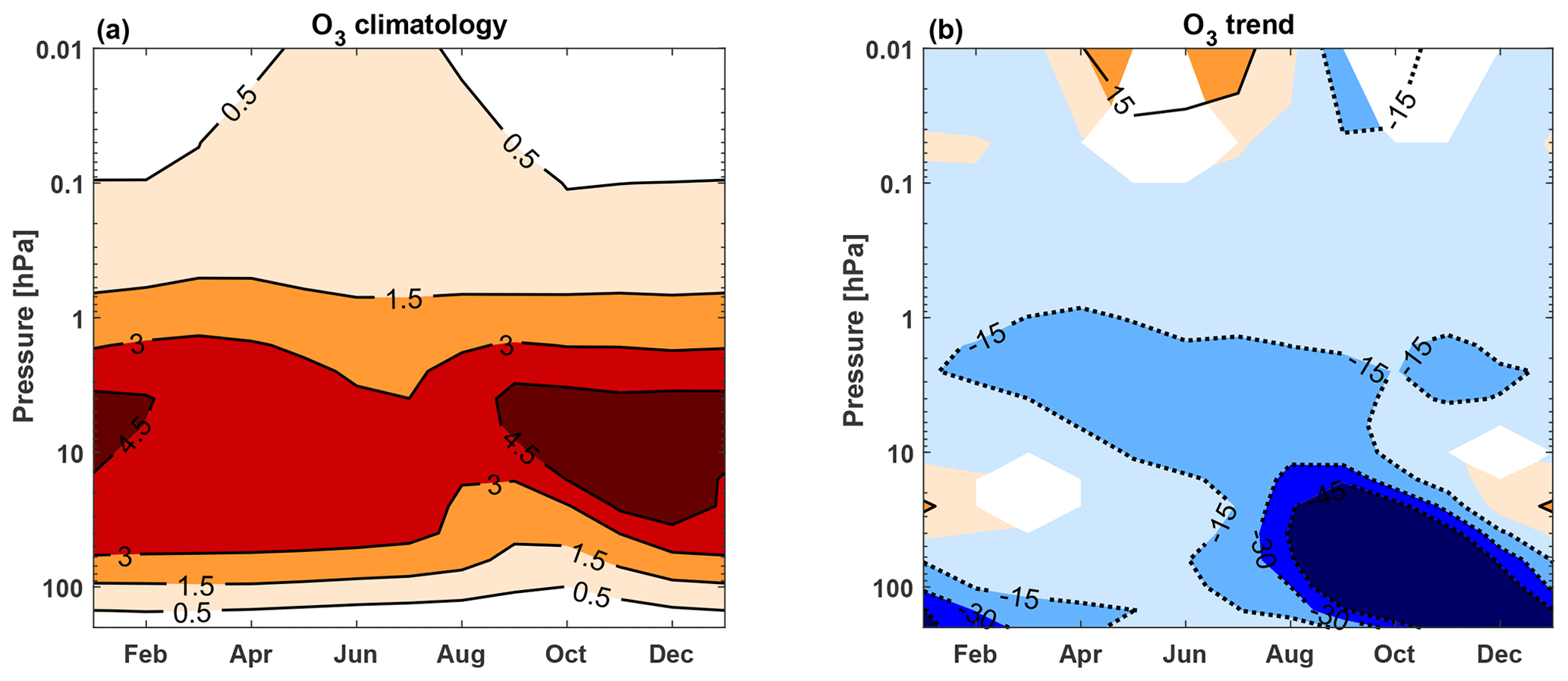
Figure 1 (a) Zonal mean ozone climatology in the Antarctic (70–90^∘ S, 0.01–200 hPa) during 1958–2008. Contour levels are 0.5, 1.5, 3 and 4.5 parts per million (ppm). (b) Zonal mean ozone trend in the Antarctic (70–90^∘ S, 0.01–200 hPa) during 1958–2008. Positive contour level (solid line) is 15 %, and negative contour levels (dotted lines) are −15 %, −30 % and −45 %. Colour shading indicates areas significant at the 95 % level, calculated with a Mann–Kendall test and a false detection rate. Figures were made using the reference simulation (see details in “Data and methods”).

Polar ozone can also be destroyed catalytically by reactive nitrogen oxides (NO_x = NO + NO₂) via reactions:

$$\begin{array}{}\text{(R6)}& {\displaystyle }{\mathrm{NO}}_{\mathrm{2}}+\mathrm{O}\to \mathrm{NO}+{\mathrm{O}}_{\mathrm{2}}\text{(R7)}& {\displaystyle }\mathrm{NO}+{\mathrm{O}}_{\mathrm{3}}\to {\mathrm{NO}}_{\mathrm{2}}+{\mathrm{O}}_{\mathrm{2}}.\end{array}$$

This reaction chain peaks at 45 km altitude (Lary, 1997). One of the main sources of polar NO_x is energetic electron precipitation (EEP) from the magnetosphere, which ionises the polar thermosphere and the upper mesosphere (Mironova et al., 2015; Nesse Tyssøy et al., 2019). In addition, sporadic solar proton events (SPEs) can produce NO_x in the mesosphere/upper stratosphere (Jackman et al., 2009). During winter, polar regions remain in darkness, which prolongs the chemical lifetime of NO_x (Solomon et al., 1982; Funke et al., 2014). Furthermore, downward vertical residual circulation in the wintertime transports polar NO_x to stratospheric altitudes (Seppälä et al., 2007; Maliniemi et al., 2020). It has been shown that this indirect stratospheric NO_x can deplete ozone by 10 %–15 % in the Antarctic upper stratosphere during winter (Semeniuk et al., 2011; Damiani et al., 2016; Arsenovic et al., 2019). Galactic cosmic rays (GCRs) also impact atmospheric NO_x and ozone. Their ionisation peaks around 10–15 km, affecting the upper troposphere/lower stratosphere region directly (Calisto et al., 2011; Jackman et al., 2016).

Reactive NO_x gases also interact with stratospheric ClO via reactions:

$$\begin{array}{}\text{(R8)}& {\displaystyle }\mathrm{ClO}+{\mathrm{NO}}_{\mathrm{2}}+M\to {\mathrm{ClONO}}_{\mathrm{2}}+M\text{(R9)}& {\displaystyle }\mathrm{ClO}+\mathrm{NO}\to \mathrm{Cl}+{\mathrm{NO}}_{\mathrm{2}}.\end{array}$$

Reaction (R8) stores both reactive nitrogen and chlorine into a reservoir agent (Lary, 1997), and thus buffers the ozone destruction associated with both NO_x and ClO. Reaction (R9) couples catalytic ozone destruction cycles of chlorine and NO_x (Brasseur and Solomon, 2005). The formation of hydrogen chloride (HCl) via reactions with HO_x can also be important for energetic particle precipitation (EPP) impacts:

$$\begin{array}{}\text{(R10)}& {\displaystyle }\mathrm{ClO}+\mathrm{OH}\to \mathrm{HCl}+{\mathrm{O}}_{\mathrm{2}}\text{(R11)}& {\displaystyle }\mathrm{ClO}+\mathrm{OH}\to \mathrm{Cl}+{\mathrm{HO}}_{\mathrm{2}}\text{(R12)}& {\displaystyle }\mathrm{Cl}+{\mathrm{HO}}_{\mathrm{2}}\to \mathrm{HCl}+{\mathrm{O}}_{\mathrm{2}}.\end{array}$$

EPP is known to produce hydrogen oxides (HO_x) in the mesosphere (Verronen et al., 2011) and direct SPE production can reach the upper stratosphere (Jackman et al., 2009). While the HO_x lifetime is too short for any EPP indirect stratospheric HO_x, the formation of HNO₃ in reaction between NO₂ and OH and its subsequent descent to stratospheric altitudes during polar nights might also play a role (Verronen and Lehmann, 2015). Finally, the reaction

$$\begin{array}{}\text{(R13)}& \mathrm{Cl}+{\mathrm{CH}}_{\mathrm{4}}\to \mathrm{HCl}+{\mathrm{CH}}_{\mathrm{3}}\end{array}$$

can also be important following Reaction (R9) (Brasseur and Solomon, 2005).

A recent study showed that satellite observations of Antarctic ClO correlated negatively with the geomagnetic activity during springtime (Gordon et al., 2021). This implies that ozone depletion by polar NO_x is modulated by chlorine loading, especially during the CFC era. Similarly, stratospheric indirect NO_x will modulate ozone depletion by ClO. In this paper, we investigate how the interaction between NO_x, ClO and ozone, and the emergence of the CFC era modulate the particle precipitation impact on ozone, by using a free-running chemistry–climate simulation with implemented particle precipitation forcing over the entire 20th century.

2 Data and methods

The chemistry–climate model SOCOL3‐MPIOM (Stenke et al., 2013; Muthers et al., 2014) consists of three interactively coupled components. The atmospheric component is the general atmospheric circulation model ECHAM5.4 (Roeckner et al., 2003), used here in configuration with T31 spectral horizontal truncation (approximately 3.75^∘ × 3.75^∘) and 30 vertical levels from the surface to 0.01 hPa (∼ 80 km). ECHAM5.4 is used in free-running mode with prescribed quasi-biannual oscillation (QBO) in the zonal wind, as the model cannot generate the QBO with the applied vertical resolution. The chemistry module MEZON (Egorova et al., 2003) computes the tendencies of 41 gas species, including 200 gas phases, 16 heterogeneous and 35 photolytic reactions. The oceanic component is MPIOM (Marsland et al., 2003), used in the nominal horizontal resolution of 3^∘, with 40 vertical layers from the ocean surface to the bottom.

The solar radiation input is based on the study by Shapiro et al. (2011). The precipitating energetic particles are prescribed following the Coupled Model Intercomparison Project Phase 6 (CMIP6) recommendations (Matthes et al., 2017). Medium-energy electrons (>30 keV) are implemented as daily ionisation rates, while auroral electrons (<30 keV) are represented as NO influx through the model top (Funke et al., 2016). SPEs and GCR are also implemented as daily ionisation rates. The tropospheric aerosols originate from the NCAR Community Atmospheric Model (CAM3.5) simulations, with a bulk aerosol model forced with the Community Climate System Model 3 sea surface temperatures. The concentrations of greenhouse gases, ozone-depleting substances and ozone precursors (CO and NO_x) follow historic values (Meinshausen et al., 2011).

In this study, the experiment simulation (EXP) contains all energetic particle precipitation sources (EEP + SPE + GCR) along with all other forcings, while the reference simulation (REF) contains all forcings apart from the particle precipitation sources. The total simulation length is 109 years (1900–2008). The time series of geomagnetic activity (the EEP ionisation model is based on the Ap index, Matthes et al., 2017), SPEs and GCR can be seen in Fig. 2. One can see a clear increase in geomagnetic activity from the early 1900s to 1960s, in agreement with the grand solar maximum. This is also seen in the cosmic ray ionisation, which reached the centennial minimum at the same time (the stronger heliospheric magnetic field is able to shield cosmic rays more efficiently). The frequency of the SPEs does not have any clear trend. One must note though that the SPE and GCR ionisation before the 1960s is only estimated indirectly based on the overall solar activity (Matthes et al., 2017). An 11-member ensemble was generated by varying initial CO₂ concentrations with 0.1 % among the different members of EXP and REF.

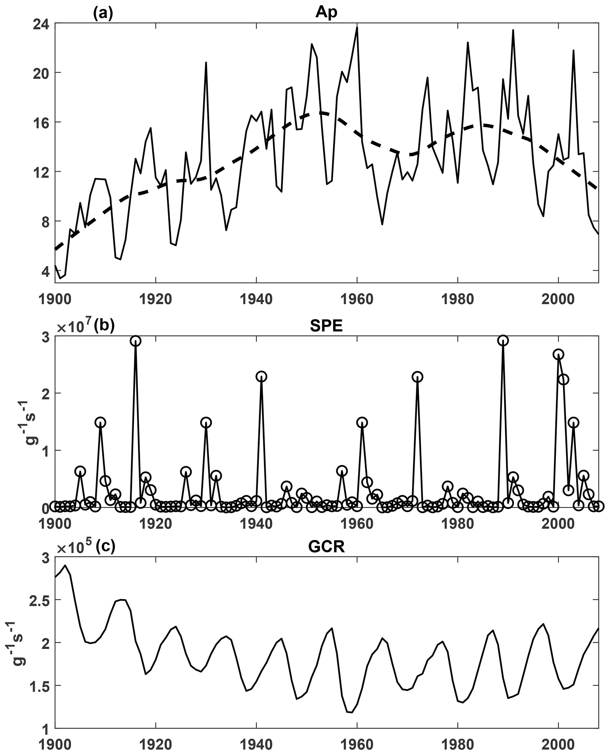
Figure 2 (a) Annual time series of geomagnetic activity index Ap (solid line) and 31-year smooth trend (dotted line). (b) Annual time series of SPEs (ion pair production rate at 1 hPa, 70–90^∘ S). (c) Annual time series of GCR (ion pair production rate at 100 hPa, 70–90^∘ S).

For atmospheric parameters, we compute zonal averages, obtain their monthly latitude–height profiles and analyse the EPP response (EXP − REF). We concentrate on volume mixing ratios of NO_x, ClO, ClONO₂, HCl and ozone. The significance in each lat–height bin is calculated with a Monte Carlo simulation. We combine ensembles from both EXP and REF (22 total), and randomly take two 11-ensemble data collections 10 000 times. These two randomly picked data matrices are subtracted similarly as the original data in each lat–height grid. The original value (EXP − REF) is compared to the distribution of these 10 000 repetitions to obtain the fraction of more extreme differences (both tails of the distribution). This fraction then represents the p value in each lat–height bin with the null hypothesis that there is no difference between EXP and REF.

Results presented in a latitude–height grid are usually spatially correlated and represent a multiple hypothesis testing situation (Wilks, 2016). Thus, simply presenting significance in each bin based on individual hypothesis testing will lead to an overestimation of the true number of rejected null hypotheses. The average number of false positives is n⋅p, where n is the number of hypothesis tests and p is the used p value. This is due to the definition of the p value and also the dependency of the neighbouring grid points, i.e. the spatial autocorrelation (Wilks, 2016). To overcome this issue, the false discovery rate is calculated for each case. It reduces the probability of false positives in line with the applied new p value limit. After the procedure, the p value can be interpreted as being the probability to obtain a false rejection of a null hypothesis. Details of the method can be found in Wilks (2016). We have used the p value limit of 0.05, which then represents 95 % probability of not having any false positives.

Figure 1 shows the relative change in ozone over the Antarctic from 1958 to 2008 in the REF simulation, calculated by subtracting a five-year mean centred on 1960 from a five-year mean centred on 2006. Significance is calculated using a Mann–Kendall test (Mann, 1945) and a false discovery rate. The smooth long-term variations shown in Fig. 2 and the following Figs. 7–10 are calculated using the LOWESS (LOcally WEighted Scatterplot Smoothing) method applied with a 31-year window (Cleveland and Devlin, 1988). More details of the method can be found in Maliniemi et al. (2014).

3 Results

3.1 Global NO_x, ClO and O₃ responses to EPP during 1979–2008

Figure 3 shows the monthly NO_x volume mixing ratio increase in the mesosphere and the stratosphere due to the EPP forcing during 1979–2008. NO_x reaches stratospheric altitudes (below 1 hPa) in the polar regions during the local winter. This is mainly due to EEP and to a lesser extent caused by SPEs (Maliniemi et al., 2020); e.g. there were only 3–4 notable SPEs during 1979–2008 as seen in Fig. 2b. In the Antarctic stratosphere, a substantial increase of NO_x is obtained from May until February, reaching roughly 20–30 hPa by late winter/spring. In the Arctic stratosphere, the lowest altitude is slightly higher, around 10 hPa during March.

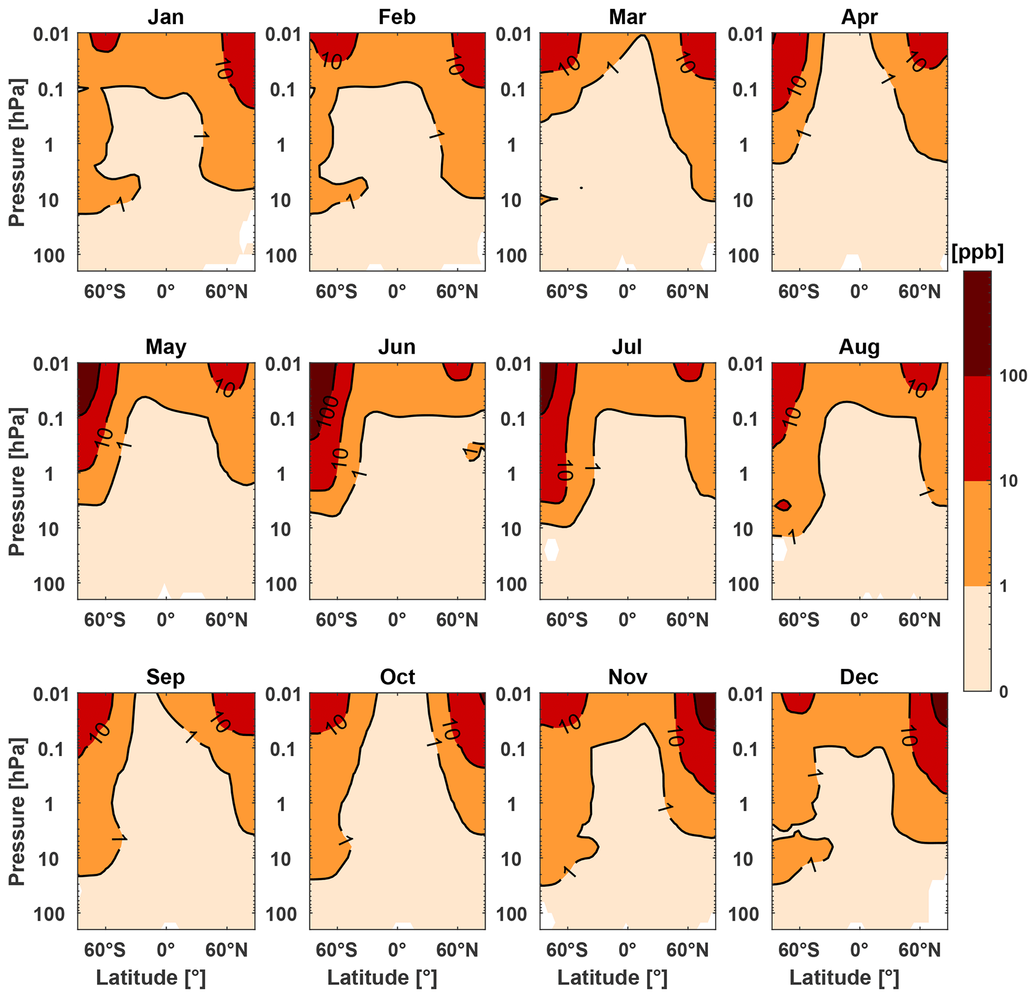
Figure 3 Absolute difference in the monthly zonal mean NO_x between EXP and REF during 1979–2008. Positive contour levels are 1, 10 and 100 parts-per-billion (ppb). The altitude range is from 0.01 to 200 hPa. Colour shading indicates areas significant at the 95 % level, calculated with a Monte Carlo simulation and a false detection rate.

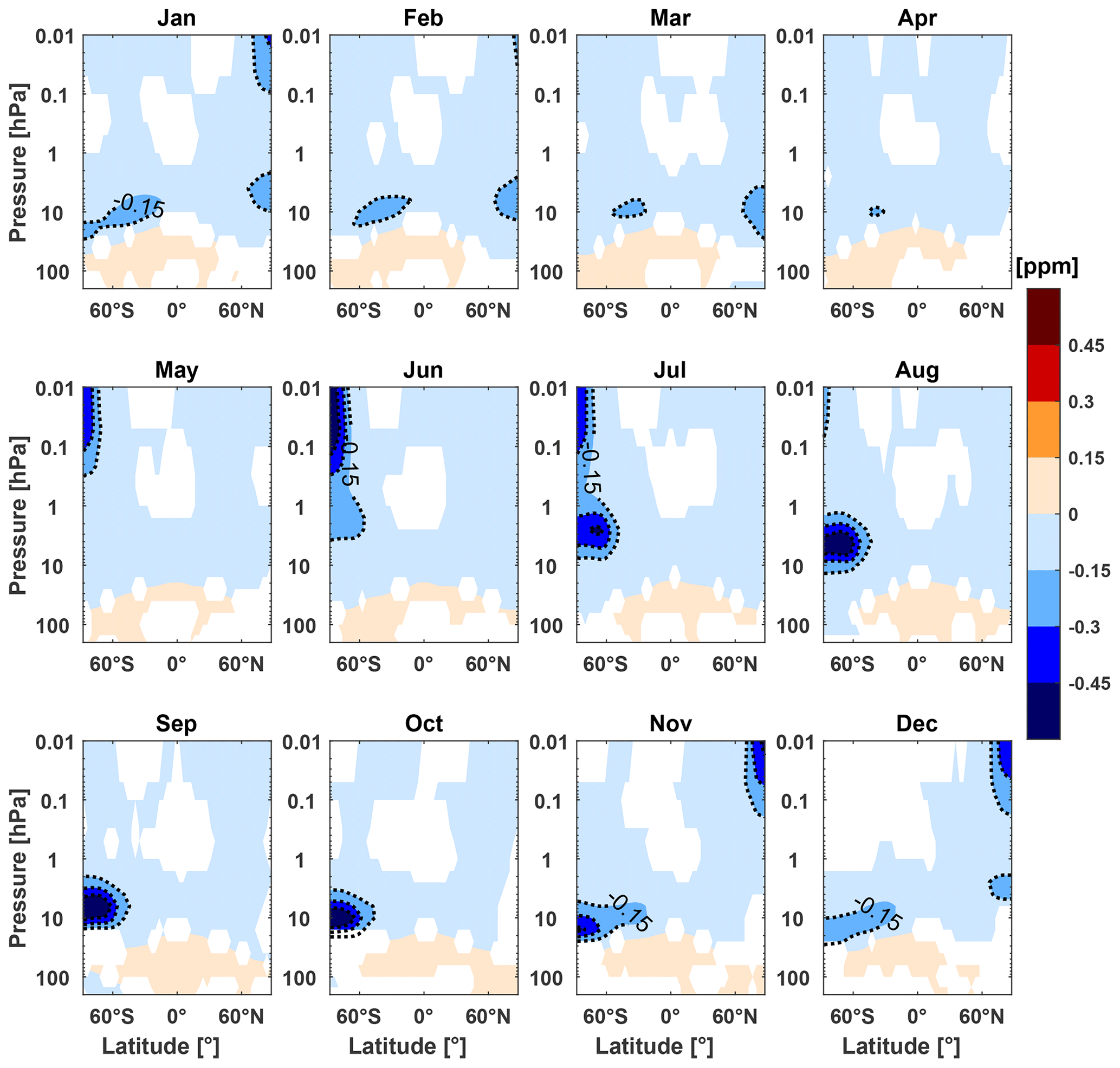
Figure 4 Absolute difference in the monthly zonal mean O₃ between EXP and REF during 1979–2008. Negative contour levels are −0.15, −0.3 and −0.45 parts per million (ppm). Colour shading indicates areas significant at the 95 % level, calculated with a Monte Carlo simulation and a false detection rate.

EPP leads to ozone depletion in the polar regions in the mesosphere and upper stratosphere, as shown in Fig. 4. Mesospheric ozone depletion is dominated by HO_x production (Jackman et al., 2008; Andersson et al., 2014; Zawedde et al., 2019). However, mesospheric ozone depletion seems to be slightly stronger in the southern hemisphere than in the Northern Hemisphere, which implies an additional dynamical or long-lived component in the Southern Hemisphere. This can be explained by a southern hemispheric polar vortex forming earlier and being more stable and less diffusive, which confines ozone depleted air more efficiently (Andersson et al., 2018). An additional explanation can also be HNO₃ formation in the mesosphere (Verronen and Lehmann, 2015). Thermospheric NO in the model is prescribed with a semi-empirical model, which, on average, has more NO entering the mesosphere in the southern hemisphere (Funke et al., 2016).

The stratospheric ozone depletion is due to NO_x catalytic Reactions (R6)–(R7) (Lary, 1997). It is larger in magnitude and lasts notably longer in the southern hemisphere than in the northern hemisphere, because the strong and stable polar vortex in the southern hemisphere isolates air mass efficiently. Seasonal evolution of the EPP ozone impact is in good agreement with earlier studies (Rozanov et al., 2012; Damiani et al., 2016). There is also a weak but significant ozone response around 100 hPa altitude covering all latitudes. It is positive and significant in the low latitudes all year and in the high latitudes during summer, but significantly negative during winter/spring, at least in the Antarctic. This Antarctic lower stratosphere response is also in agreement with Rozanov et al. (2012) and Damiani et al. (2016). Consistently positive weak ozone responses in the lower stratosphere are a consequence of GCR (Calisto et al., 2011; Jackman et al., 2016), while it is likely dominated by the indirect EPP effect in the high latitudes during winter.

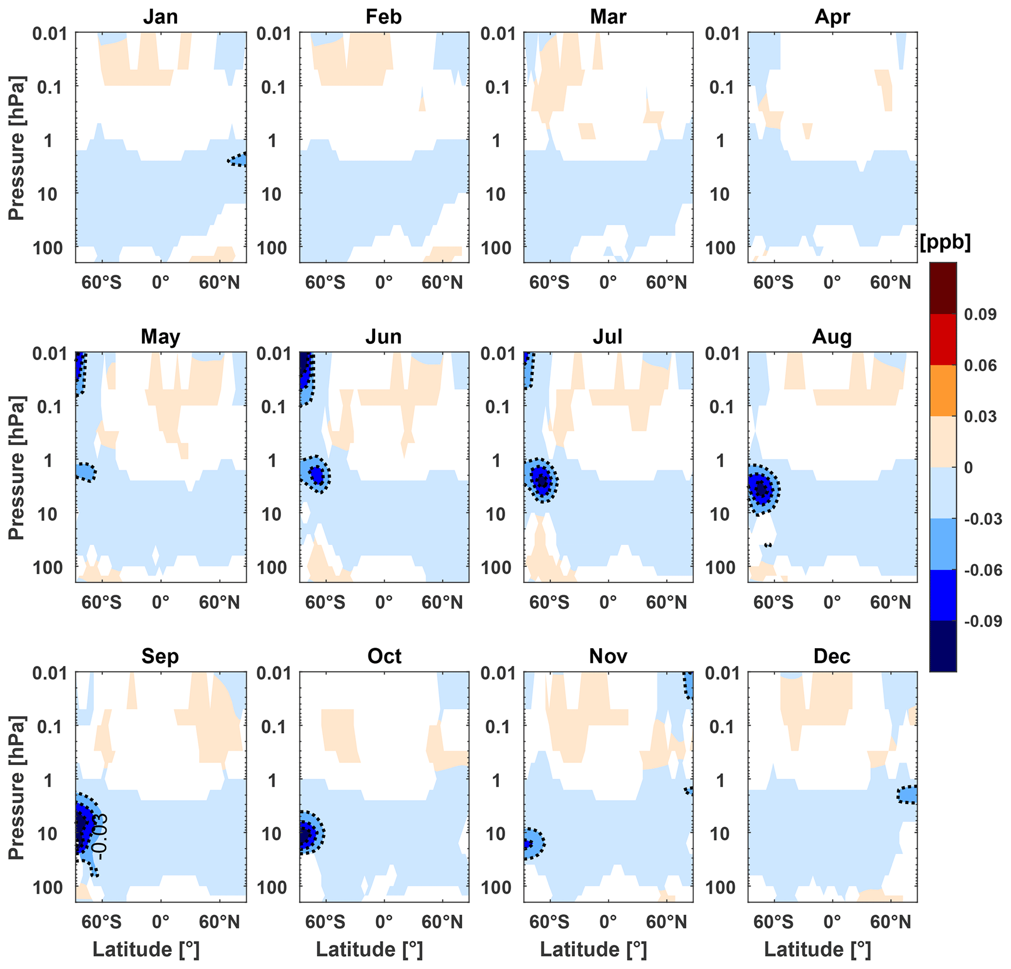
Figure 5 Absolute difference in the monthly zonal mean ClO between EXP and REF during 1979–2008. Negative contour levels are −0.03, −0.06 and −0.09 ppb. Colour shading indicates areas significant at the 95 % level, calculated with a Monte Carlo simulation and a false detection rate.

Figure 5 shows a monthly ClO volume mixing ratio related to the EPP forcing. The altitude of polar ClO decreases in the southern hemisphere agrees well with the lowest altitude of NO_x increases during May–November. There is a substantial decrease of ClO below 1 hPa from June to November in the Antarctic stratosphere, which extends down to 30 hPa in springtime, matching the pattern of descending NO_x. As explained above, NO_x and ClO can interact with Reactions (R8) and (R9) (HO_x and ClO via Reactions R10–R12), interfering with the catalytic ozone-destroying cycles of both agents. Interestingly, there are weak but significantly positive ClO responses in the Antarctic at 100 hPa altitude during winter (June to September).

3.2 Antarctic NO_x, ClO and O₃ responses to EPP over the 20th century

Figure 6 shows the Antarctic polar climatologies of NO_x, ClO, ClONO₂ and HCl during 1979–2008 from the REF simulation. Small values are denoted in all variables below 200 hPa (not shown). Furthermore, ClO and ClONO₂ have small values above the stratopause (roughly 1 hPa).

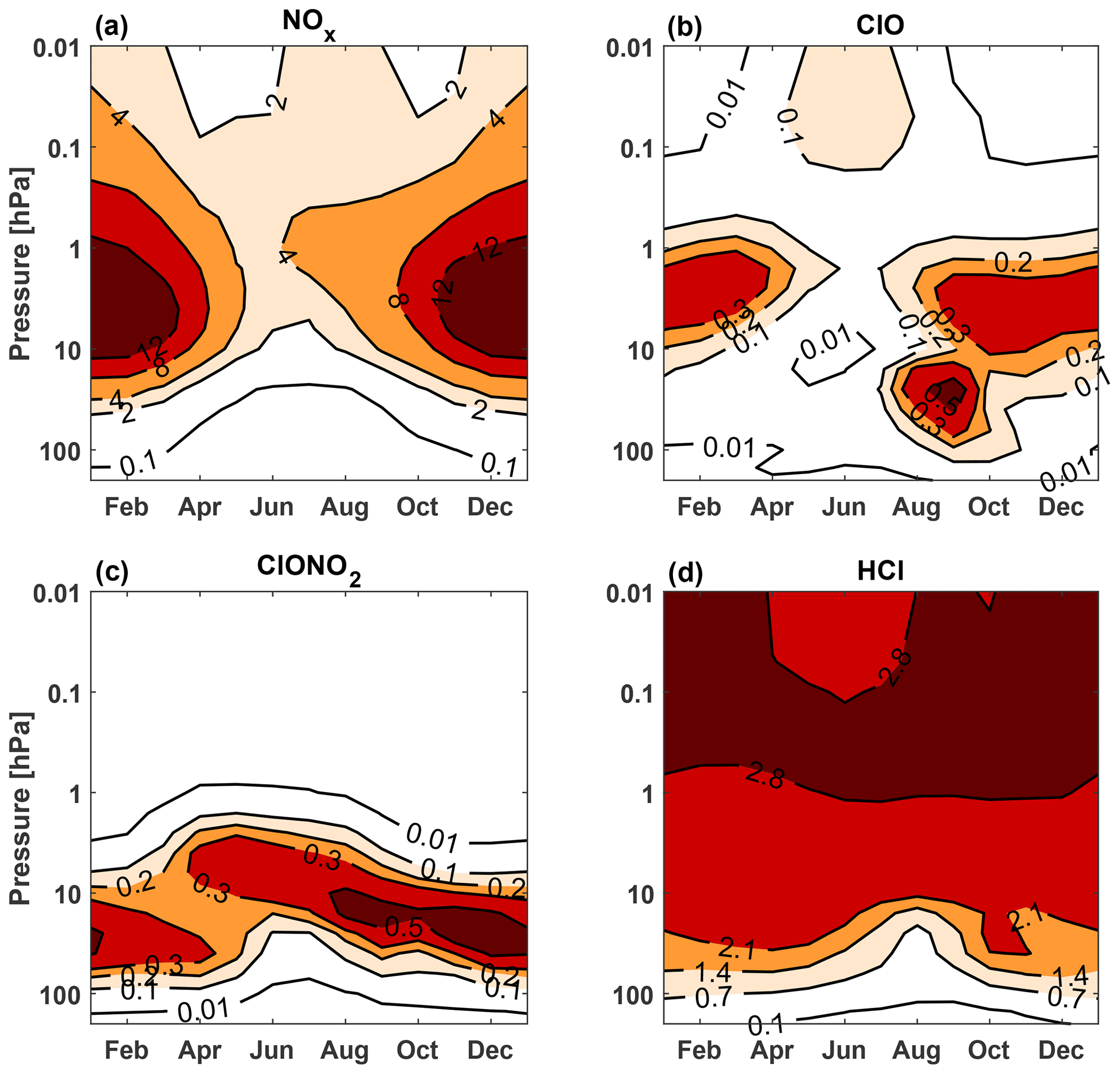
Figure 6 (a) Seasonal climatology of NO_x in the Antarctic (70–90^∘ S, 0.01–200 hPa) during 1979–2008. Positive contour levels are 0.1, 2, 4, 8 and 12 ppb. Seasonal climatology for (b) ClO and (c) ClONO₂ are shown with positive contour levels of 0.01, 0.1, 0.2, 0.3 and 0.5 ppb, and for (d) HCl with positive contour levels of 0.1, 0.7, 1.4, 2.1 and 2.8 ppb. All figures are calculated using the REF simulation, i.e. without the EPP forcing.

A seasonally varying NO_x increase in the Antarctic stratosphere due to EPP is shown in Fig. 7a. In addition, September–October NO_x abundance at 10–20 hPa in EXP and REF are compared over the whole 20th century in Fig. 7b and c. An increase of NO_x of more than a hundred percent is present in the upper stratosphere during winter. NO_x descends below 10 hPa by July and a more than 50 % increase is sustained until November when the polar vortex typically breaks down. There is also a relative increase of NO_x around 50–100 hPa during June–September. This is directly related to GCR and partly to EEP/SPE from the previous season (a more than 15 % increase continues descending after November). A similar increase at these altitudes during mid-winter is also obtained in Rozanov et al. (2012).

The 10–20 hPa NO_x time series for September–October shows that there is a consistent negative trend over the whole 20th century in REF, possibly a consequence of increasing chemical destruction of NO_x in the cooler stratosphere (Stolarski et al., 2015). The NO_x time series in EXP is mostly affected by the EEP/geomagnetic activity (Fig. 2a). The Spearman rank correlation coefficient between EXP NO_x in Fig. 7b and the annual Ap index is 0.73 (p value < 0.01). The Spearman correlation between EXP − REF NO_x in Fig. 7c and the annual Ap index is 0.84. However, there is also a negative trend in the EXP NO_x time series after 1960 in Fig. 7b. The EXP NO_x level at the end of the simulation is lower than in the beginning, despite higher geomagnetic activity in the early 21st century compared to the early 20th century.

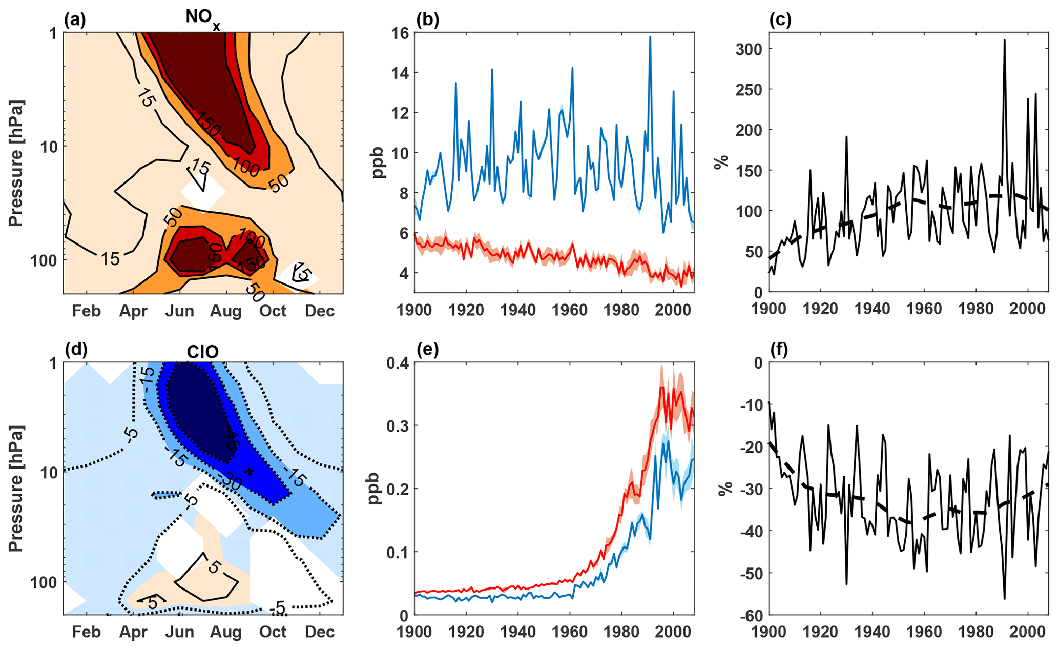
Figure 7 (a) Relative difference $(\text{EXP}-\text{REF})/\mathrm{REF}$ in the monthly zonal mean polar NO_x (70–90^∘ S, 1–200 hPa) during 1979–2008. Positive contour levels are 15 %, 50 %, 100 % and 150 %. Colour shading indicates areas significant at the 95 % level calculated with a Monte Carlo simulation and a false detection rate. (b) September–October ensemble mean time series of polar NO_x (70–90^∘ S, 10–20 hPa) in EXP (blue) and REF (red). Shaded light blue and red areas represent 95 % confidence intervals of ensemble means. (c) Relative difference of EXP and REF (solid line) and 31-year smooth trend (dotted line). (d) Polar ClO with negative contour levels of −5 %, −15 %, −30 %, −45 % (dotted lines) and a positive contour level of 5 % (solid line). (e, f) This is the same for ClO as (b) and (c), respectively.

Figure 7d shows relative changes in Antarctic stratospheric ClO due to the EPP forcing. A more than 45 % decrease in ClO is obtained between EXP and REF in mid-winter, between 1 and 10 hPa in Fig. 7d. A more than 15 % ClO decrease in EXP relative to REF continues well into spring, extending down to 40 hPa.

The mid-stratospheric ClO time series in September–October (Fig. 7e and f) shows that there has been a strong increase in chlorine since 1960, due to CFC emissions. However, the ClO amount in EXP consistently falls below the amount in REF. The relative difference between EXP and REF is anticorrelating with the level of geomagnetic activity ($R=-\mathrm{0.46}$, p value < 0.01), rather than being dependent on the overall amount of ClO. ClO is reduced by 30 %–40 %, with the EPP forcing at 10–20 hPa in September–October after the 1950s.

Interestingly, significant positive ClO responses to EPP forcing at 50–100 hPa are present during winter months in Fig. 7d. This occurs at altitudes where polar stratospheric clouds (PSCs) form in the Antarctic (Pitts et al., 2018), likely being a consequence of reservoir gases breaking on PSC (Molina et al., 1987; Webster et al., 1993). The influence of EPP on these processes in the lower stratosphere is discussed in more detail below. This positive ClO response in the lower stratosphere was also seen in satellite data by Gordon et al. (2021) during August–October.

Figure 8 shows the relative changes in Antarctic stratospheric ClONO₂ and HCl due to the EPP forcing. A substantial increase of ClONO₂ in EXP relative to REF is seen in the upper stratosphere during winter (Fig. 8a). However, if compared to the climatology of ClONO₂ in Fig. 6, it is evident that at altitudes above 3 hPa, there is very little ClONO₂ and most is located between 3 and 80 hPa. Between 3 and 10 hPa, the ClONO₂ amount is less in EXP than in REF during mid-winter. This implies that reduced ClO due to EPP at this location in Fig. 7d cannot be explained by Reaction (R8), but is likely due to Reaction (R9) and the consequent formation of HCl seen in Fig. 8d (Cl reacting with methane) (Brasseur and Solomon, 2005). Reactions (R10)–(R12) with SPE produced OH and/or the formation of mesospheric HNO₃ (Verronen and Lehmann, 2015). Its subsequent descent to stratospheric altitudes during polar nights with following photolysis might partly play a role in EPP-related HCl formation.

In springtime, there is a significant ClONO₂ increase due to EPP at 10–20 hPa altitudes (Fig. 8a), which is also seen in time series Fig. 8b and c. The relative effect of EPP on ClONO₂ increases after 1960, reaching 5 % after 2000. However, a positive correlation between annual geomagnetic activity and HCl in 10–20 hPa from Fig. 8f (R=0.48, p value < 0.01) implies that ClO is converted to HCl, instead of ClONO₂ (correlation between geomagnetic activity and Fig. 8c data is −0.01 over the whole time period).

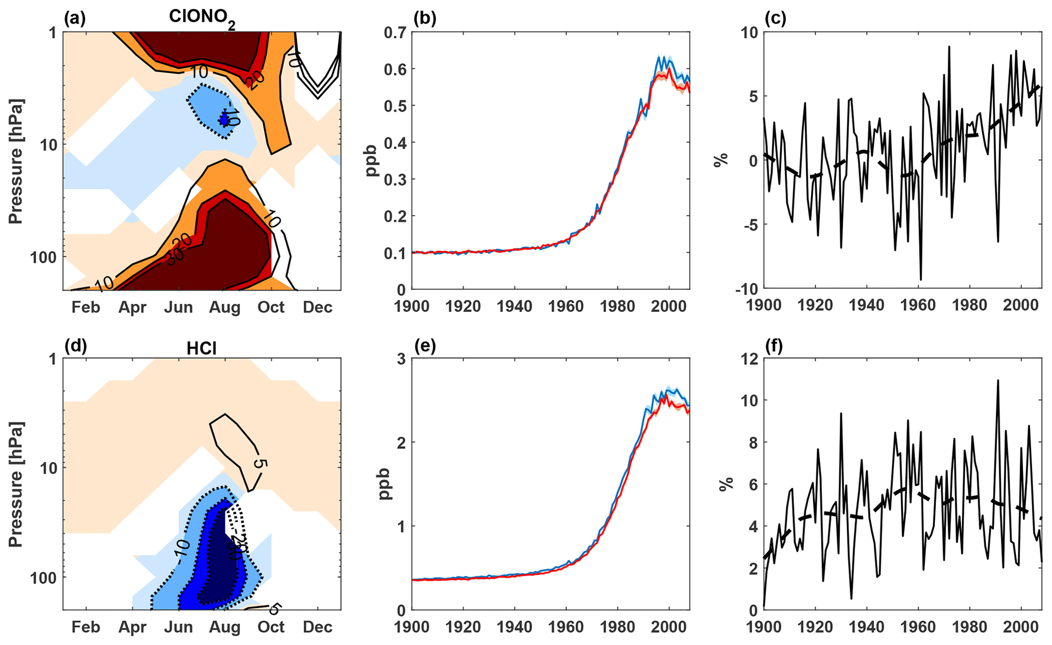
Figure 8 (a) Relative difference $(\text{EXP}-\text{REF})/\mathrm{REF}$ in the monthly zonal mean polar ClONO₂ (70–90^∘ S, 1–200 hPa) during 1979–2008. Positive contour levels (solid lines) are 10 %, 20 % and 30 % and the negative contour level (dotted line) is −10 %. Colour shading indicates areas significant at the 95 % level, calculated with a Monte Carlo simulation and a false detection rate. (b) September–October ensemble mean time series of polar ClONO₂ (70–90^∘ S, 10–20 hPa) in EXP (blue) and REF (red). Shaded light blue and red areas represent 95 % confidence intervals of ensemble means. (c) Relative difference of EXP and REF (solid line) and 31-year smooth trend (dotted line). (d) Polar HCl with negative contour levels of −10 %, −20 % and −30 % (dotted lines) and positive contour level of 5 % (solid line). (e, f) This is the same for HCl as (b) and (c), respectively.

There is also a significant and strong increase of ClONO₂ in the lower stratosphere during winter in Fig. 8a, accompanied by a significant decrease of HCl in Fig. 8d. It implies that EPP is able to interact with the mechanism of ClO release from ClONO₂ and HCl on PSC (Molina et al., 1987; Webster et al., 1993). ClO is mostly released by consuming HCl, which recovers slowly to initial values, while ClONO₂ levels can rebuild fairly quickly and to excess levels of its initial values (Molina et al., 1987; Webster et al., 1993), especially in the presence of additional NO_x due to EPP. This means that EPP keeps the heterogeneous processing between HCl and ClONO₂ running and results in less HCl, more ClONO₂ and finally, more ClO via processing on PSCs.

The relative effect of EPP on Antarctic ozone shows a 10 %–15 % decrease in the upper and mid-stratosphere from mid-winter until November (Fig. 9a). The time series of mid-stratospheric (10–20 hPa) ozone in both EXP and REF during September–October (Fig. 9b) show a negative trend since 1960, but it is notably weaker in EXP. The relative difference between EXP and REF (Fig. 9c) shows that the trend correlates negatively with the overall geomagnetic activity before the CFC era (Spearman correlation $R=-\mathrm{0.65}$, p value < 0.01 during 1900–1960). After 1960, the effect of EPP on ozone at 10–20 hPa diverges away from the overall geomagnetic activity level ($R=-\mathrm{0.07}$, p value = 0.65 during 1961–2008). At the beginning of the 21st century, average ozone depletion due to EPP at 10–20 hPa is just a few percent and is notably less than in the early 20th century (10 % to 15 %), while geomagnetic activity in the early 21st century is roughly at the level of the 1920s/1930s (Fig. 2).

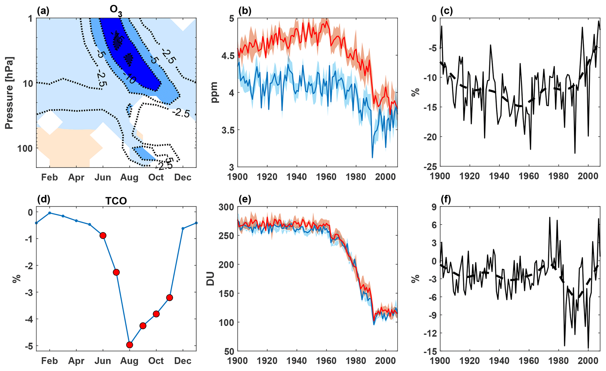
Figure 9 (a) Relative difference $(\text{EXP}-\text{REF})/\mathrm{REF}$ in the monthly zonal mean polar ozone (70–90^∘ S, 1–200 hPa) during 1979–2008. Negative contour levels (dotted lines) are −2.5 %, −5 %, −10 % and −15 %. Colour shading indicates areas significant at the 95 % level, calculated with a Monte Carlo simulation and a false detection rate. (b) September–October ensemble mean time series of polar ozone (70–90^∘ S, 10–20 hPa) in EXP (blue) and REF (red). Shaded light blue and red areas represent 95 % confidence intervals of ensemble means. (c) Relative difference of EXP and REF (solid line) and 31-year smooth trend (dotted line). (d) Relative effect of EPP on polar total column ozone (TCO). Red circles represent months with significant differences at the 95 % level, calculated with a Monte Carlo simulation and a false detection rate. (e, f) This is the same for TCO as (b) and (c), respectively.

Figure 9a also shows a significant ozone depletion by EPP around 100 hPa altitude during August–October. This is in agreement with ClO increases seen in Fig. 7d at same altitude earlier in winter. When the polar night ends, ClO released by PSCs depletes ozone via the ClO dimer cycle (Reactions R3–R5) (Lary, 1997).

The relative effect of EPP on Antarctic total column ozone (TCO) during 1979–2008 is shown in Fig. 9d. It shows a 4 % to 5 % decrease in spring (August–October). When considering the effect on TCO over the whole century in September–October (Fig. 9f), it has an average of around 1 %–3 % reduction until the 1980s, after which it becomes notably stronger. To understand this evolution in TCO, Fig. 10 shows the 1900–2008 time series of August–October ozone at 100 hPa. The relative ozone effect at 100 hPa by EPP is mostly positive (Calisto et al., 2011) until 1980, after which it decreases to a minus 5 %–10 % level in Fig. 10d. This is a very different evolution than in the mid-stratosphere in Fig. 9c. On the other hand, the EPP effect on TCO after 2000 returns to similar levels compared to before 1980 and seems to be above zero at the end of the simulation. Gordon et al. (2021) showed a positive correlation between geomagnetic activity and polar TCO in springtime (October–November) during 2005–2017. The Spearman correlation between geomagnetic activity and EXP polar TCO during October–November 1998–2008 is also slightly positive, but insignificant (R=0.21, p value = 0.54). This positive TCO response is likely due to a reduction in mid-stratospheric ozone depletion, as seen in Fig. 9c (note that there is roughly an order of magnitude difference in ozone abundance between 10–20 and 100 hPa in Figs. 9b and 10c).

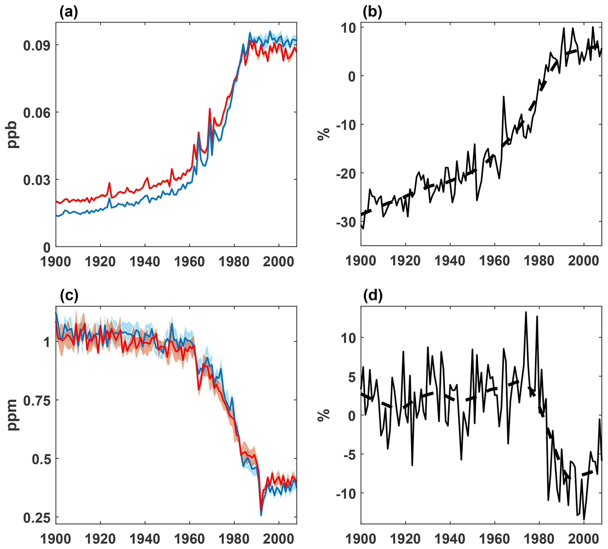
Figure 10 (a) July–September ensemble mean time series of polar ClO (70–90^∘ S, 100 hPa) in EXP (blue) and REF (red). The shaded light blue and red areas represent 95 % confidence intervals of ensemble means. (b) Relative difference of ClO EXP and REF (solid line) and 31-year smooth trend (dotted line). (c) August–October ensemble mean time series of polar O₃ (70–90^∘ S, 100 hPa) in EXP (blue) and REF (red). Shaded light blue and red areas represent 95 % confidence intervals of ensemble means. (d) The relative difference of O₃ EXP and REF (solid line) and 31-year smooth trend (dotted line).

The absolute ClO time series at 100 hPa seen in Fig. 10a increases substantially after 1960. Interestingly, the relative difference between EXP and REF (Fig. 10b) follows the overall level of ClO (and CFC emissions), and is a very different than in the mid-stratosphere in Fig. 7f.

To understand this change of sign in lower stratospheric ClO response to EPP, we analyse the seasonal variability of 100 hPa $\mathrm{NO}/{\mathrm{NO}}_{\mathrm{2}}$ ratio, ClO, HCl and ClONO₂ responses between low and high chlorine loading in Fig. 11. The time periods of 1924–1934 (low chlorine) and 1997–2007 (high chlorine) were chosen since they represent roughly similar geomagnetic activity levels (see Fig. 2a) during solar cycles 16 and 23, respectively. One can see that the $\mathrm{NO}/{\mathrm{NO}}_{\mathrm{2}}$ ratio starting from June is notably higher during the CFC era (Fig. 11b) than in the pre-CFC era (Fig. 11a). A potential explanation for this is the lower ozone amount, which reduces Reaction (R7) and increases the $\mathrm{NO}/{\mathrm{NO}}_{\mathrm{2}}$ ratio. There is generally more NO_x available (due to EPP) to react with ClO_x. In the pre-CFC era, the low $\mathrm{NO}/{\mathrm{NO}}_{\mathrm{2}}$ ratio favours ClONO₂ reformation (Reaction R8) after a heterogeneous reaction between HCl and ClONO₂ (Fig. 11c), resulting in less ClO and more ClONO₂ due to EPP (Fig. 11e). Thus, heterogeneous processing on PSCs is HCl-limited in the pre-CFC era (Fig. 11c). In the CFC era, higher $\mathrm{NO}/{\mathrm{NO}}_{\mathrm{2}}$ ratio limits ClONO₂ reformation and allows active chlorine (and ClO) to accumulate (Fig. 11d). Heterogeneous processing is thus ClONO₂-limited. While EPP-related ClONO₂ production in the CFC era is also slowed due to a higher $\mathrm{NO}/{\mathrm{NO}}_{\mathrm{2}}$ ratio, it is still net positive over the whole winter (Fig. 11f). This excess ClONO₂ due to EPP can keep the heterogeneous processing running, resulting in ClO increases and considerable HCl decreases over the whole winter (Fig. 11f).

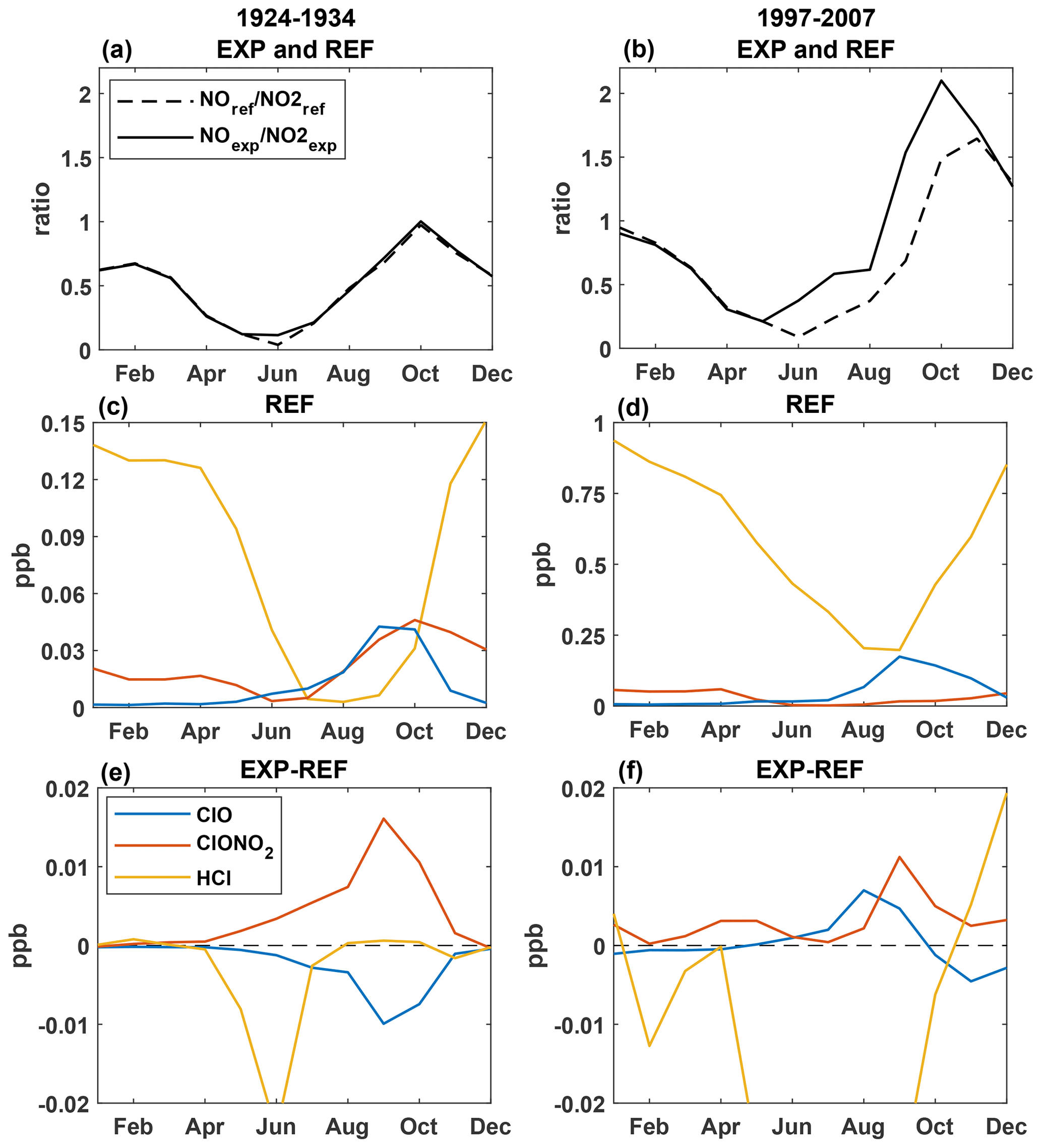
Figure 11 (a) Seasonal polar $\mathrm{NO}/{\mathrm{NO}}_{\mathrm{2}}$ ratio at 100 hPa in EXP (solid line) and REF (dashed line) during 1924–1934, and (b) during 1997–2007. (c) Seasonal REF polar 100 hPa climatology of ClO (blue), HCl (yellow) and ClONO₂ (red) during 1924–1934, and (d) during 1997–2007. Note the different y axes in (c) and (d). (e) Seasonal EXP − REF polar ClO (blue), HCl (yellow) and ClONO₂ (red) at 100 hPa during 1924–1934, and (f) during 1997–2007.

Positive ClO response in the lower stratosphere due to EPP was also found by Gordon et al. (2021). Damiani et al. (2016) showed a negative ozone response at the same altitudes related to EPP; however, they were related to regression analysis with the geomagnetic activity. We note that it can be difficult to point to the exact source (direct effect by GCR or indirect effect from above by EEP/SPE) in regression studies, due to the somewhat high collinearity between geomagnetic activity and GCR on interannual scales (Maliniemi et al., 2019). Jackman et al. (2009) showed that nitrogen species (NO_y) and ClONO₂ produced by SPE survive long enough to descend to 100 hPa altitude several months after the initial event. These results support that the ClO response seen in the lower stratosphere is likely a combination of both EEP/SPE and GCR. We also note that this lower stratospheric ClO/ozone signal is not related to dynamics, i.e. any indirect effects of EPP on the polar vortex and meridional circulation. No notable or significant zonal wind responses (EXP − REF) during winter 1979–2008 was found (not shown).

4 Summary

This study verifies the significant polar stratospheric ozone depletion by EPP during winter over the whole 20th century. The ozone depletion in the upper and mid-stratosphere is a consequence of mostly EEP/geomagnetic activity and partly SPE producing NO_x in the thermosphere and the mesosphere, which then descends to stratospheric altitudes during winter (Seppälä et al., 2007; Funke et al., 2014). In the Antarctic during 1979–2008, ozone depletion varies from more than 10 % in the winter upper stratosphere to 5 %–10 % in the spring mid and lower stratosphere between EXP and REF simulations. This is largely in agreement with previous studies (Rozanov et al., 2012; Damiani et al., 2016). The effect of EPP on Antarctic total column ozone is a few percent reduction during August to October, though it diminishes close to zero percent at the end of the simulation.

However, the Antarctic ozone depletion is modulated during the latter half of the 20th century, especially during springtime. The ozone depletion efficiency in the mid-stratosphere weakens towards the beginning of the 21st century. Decadal geomagnetic activity decline in the late 20th century cannot solely account for this weaker ozone depletion by EPP. Furthermore, significant ozone depletion by EPP emerges during August–October in the lower Antarctic stratosphere (100 hPa) after 1980.

We find a significant decrease of stratospheric ClO due to the EPP impact in the same altitude where NO_x is descending seasonally. The relative ClO reduction in the Antarctic upper and mid-stratosphere varies mainly with the level of geomagnetic activity over the whole century. EPP can reduce ClO by 30 % in the upper stratosphere during winter and in the mid-stratosphere during late winter/spring, even during the CFC era. ClO reduction during mid-winter between 1 and 20 hPa is mostly accounted for by an increase of HCl and partly by ClONO₂.

In the lower Antarctic stratosphere (100 hPa), ClO abundance increases relative to the model run without EPP by more than 5 % during winter after 1980, while the EPP effect on ClO before the CFC era is negative. The seasonal emergence of this ClO response after 1980 is consistent with the formation of PSCs in the Antarctic and occurs slightly before the depletion of ozone at the same altitude. Activation of chlorine from reservoir species ClONO₂ and HCl can be explained by heterogenous reactions on PSCs (Molina et al., 1987; Webster et al., 1993). We propose that during the pre-CFC era, heterogeneous processing on PSCs is HCl-limited, and excess NO_x due to EPP enhances ClONO₂ reformation via Reaction (R8), leading to lower ClO levels. However, during the CFC-era, low ozone levels limit Reaction (R7) between NO and ozone and lead to a higher $\mathrm{NO}/{\mathrm{NO}}_{\mathrm{2}}$ ratio. This limits the ClONO₂ reformation and makes heterogeneous processing ClONO₂-limited. While the EPP-related production of ClONO₂ is also slowed in the CFC era, it is still net positive over the whole winter. EPP is thus able to keep heterogeneous processing running and results in an increase of ClO and a substantial decrease of HCl. These results imply that EPP has significantly modulated chemical processes responsible for ozone hole formation.

The introduction of CFC emissions since the 1960s has significantly influenced the ozone response by EPP. With the implementation of the Montreal Protocol (Velders et al., 2007), the ClO amount in the stratosphere is expected to return to pre-CFC levels sometime after the 2050s. Based on the results presented here, we can therefore expect a higher efficiency of chemical ozone destruction by EPP in the upper stratosphere in the future. Furthermore, recent results have shown that EPP-related NO_x is increasing substantially in the future Antarctic upper stratosphere, due to stronger vertical transport under climate change (Maliniemi et al., 2020, 2021). This is happening despite the increasing chemical destruction of NO_x in the cooler stratosphere (Stolarski et al., 2015). In summary, (1) higher efficiency of chemical ozone destruction due to the declining CFC levels and (2) stronger vertical transport will make EPP-NO_x important for Antarctic upper stratospheric ozone over the coming decades. However, the evolution of ozone depletion in the Antarctic lower stratosphere by EPP is more uncertain. More research, e.g. with idealised model experiments targeting impacts on the future atmospheric state, is needed to quantify the EPP-related ozone response at these altitudes.