the Creative Commons Attribution 4.0 License.
the Creative Commons Attribution 4.0 License.
 | 17 Jun 2022
The Sun's role in decadal climate predictability in the North Atlantic
Wenjuan Huo
Katja Matthes
Kunihiko Kodera
Tim Kruschke
Despite several studies on decadal-scale solar influence on climate, a systematic analysis of the Sun's contribution to decadal surface climate predictability is still missing. Here, we disentangle the solar-cycle-induced climate response from internal variability and from other external forcings such as greenhouse gases. We utilize two 10-member ensemble simulations with a state-of-the-art chemistry–climate model, to date a unique dataset in chemistry–climate modeling. Using these model simulations, we quantify the potential predictability related to the solar cycle and demonstrate that the detectability of the solar influence on surface climate depends on the magnitude of the solar cycle. Further, we show that a strong solar cycle forcing organizes and synchronizes the decadal-scale component of the North Atlantic Oscillation, the dominant mode of climate variability in the North Atlantic region.
- Article
(5986 KB) - Full-text XML
-
Supplement
(3552 KB) - BibTeX
- EndNote


Since the middle of the last century long-term changes in global climate have been dominated by anthropogenic greenhouse gas emissions. Nevertheless, natural forcings play an important but poorly quantified role in past and present climate, especially on regional scales. Solar forcing variability has been suggested to affect regional climate variability (Gray et al., 2010) and to synchronize internal variability modes such as the North Atlantic Oscillation (NAO) (Thiéblemont et al., 2015). Consequently, solar variability may offer a source of decadal predictability for regional climate due to its periodicity (Dunstone et al., 2016; Kushnir et al., 2019).
In recent years, comprehensive (decadal or near-term) climate prediction efforts have been made to provide a skillful and reliable forecast of the actual evolution of both externally forced and internally generated components of the climate system. These prediction systems show forecast skill for several years (Bellucci et al., 2015; Yeager and Robson, 2017), and at least for large multi-model ensemble systems a robust benefit from initialization that goes beyond the externally forced climate response can be shown for a number of regions globally (Smith et al., 2019). Yet a comprehensive understanding of the predictability of the coupled climate system as well as the interaction between different predictability drivers is missing.
It is challenging to separate the 11-year solar cycle surface signal from internal climate variability in observations because the solar signal is small compared to internal variability and the number of solar cycles is limited. Investigating its detectability, a recent study (Chiodo et al., 2019) questioned the statistical reliability of the previously widely accepted solar cycle influence on North Atlantic climate which projects onto the NAO (Gray et al., 2013, 2016; Kodera, 2003; Kodera et al., 2016; Kodera and Kuroda, 2002; Matthes et al., 2006; Thiéblemont et al., 2015). The present paper intends to partly rebut the conclusions of this study and to provide new robust evidence of solar influence on North Atlantic climate, which is small but non-negligible compared to internal variability. We utilize a unique set of two 10-member ensemble simulations of a state-of-the-art coupled chemistry–climate model to isolate and decipher the 11-year solar cycle's footprint in North Atlantic surface climate variability and to quantify the contribution of the solar cycle to regional decadal potential predictability relative to other external forcings and internal variability during Northern Hemisphere winter. A similar experimental approach has been used by Andrews et al. (2015); however, our simulations are much longer and include the spectral solar irradiance as well as auroral-electron forcing from the most sophisticated solar forcing dataset currently available for climate models and recommended for CMIP6 and also include a well-resolved shortwave radiation scheme and a comprehensive module for middle-atmosphere chemistry modeling.
The chemistry–climate model in use is CESM1(WACCM) (Marsh et al., 2013). One ensemble includes the full CMIP6 solar forcing (FULL), while the other only considers the low-frequency (timescales longer than ∼ 30 years) changes in solar irradiance (LOWFREQ) (Fig. S1 in the Supplement). All simulations have been integrated over the historical period 1850–2014. We estimate the potential predictability variance fraction (ppvf) related to the 11-year solar cycle as well as to all other external forcings (including the low-frequency component of solar variability) for decadal (8-year running mean) variations in winter (DJF) surface air temperatures (see “Methods” section). Eight-year running means are chosen as these are a typical target of actual decadal prediction efforts (Goddard et al., 2013). The ppvf describes how much of the total decadal variance in our FULL ensemble is explained by the respective forcing(s). The ratio of variance that cannot be associated with any external forcing is regarded as internal variability. The extratropical North Atlantic is a hotspot of solar cycle influence on climate predictability (Fig. 1a). In some parts, up to 25 % of the decadal variance of winter surface air temperatures is explained by the solar cycle in our model. At the same time, similar parts of the North Atlantic show comparably low (<15 %) potential predictability due to other (low-frequency) external forcings (Fig. 1b) and large internal variability (>65 %) (Fig. 1c).
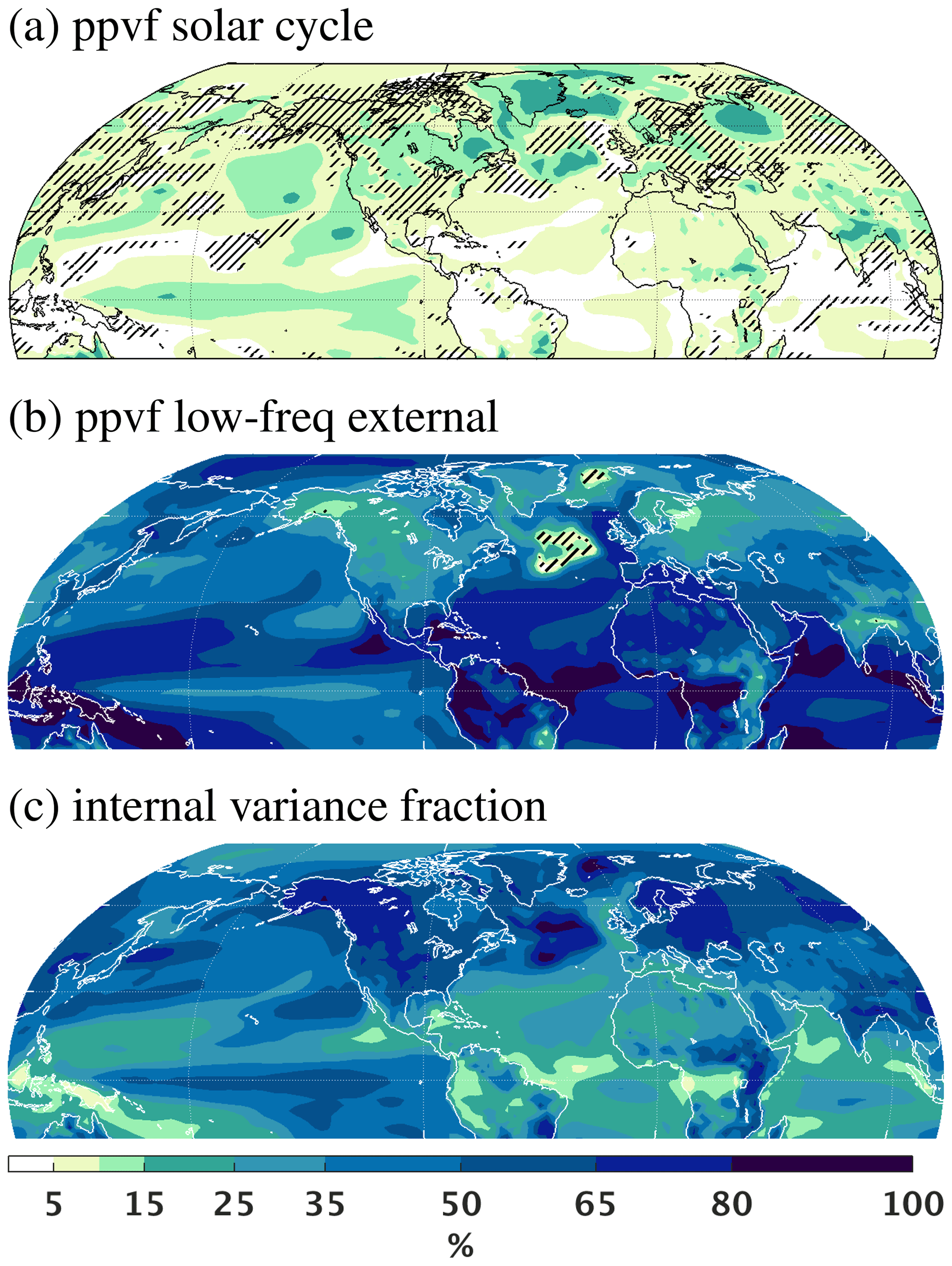
Figure 1Decadal potential predictability due to the solar cycle, other external forcings and internal climate variability. Potential predictability variance fraction (ppvf; explained variance) with respect to the DJF 8-year averaged surface air temperature associated with (a) the 11-year solar cycle, (b) all other external forcings (anthropogenic forcings, volcanic aerosols, and solar-induced low-frequency variability), and (c) remaining variance fraction due to internal climate variability. Statistically insignificant regions (p>0.05) in (a) and (b) are hatched. Panel (b) exhibits masked areas solely over a few grid points in the North Atlantic because “ppvf low-frequency external” for 2 m temperature is significant almost globally. See “Methods” section for more details on the ppvf calculation and statistical significance estimates.
The range of externally and internally generated variance fractions of our large CESM ensemble is well within the range of other high-top CMIP5 models (Fig. S2), which, however, do not distinguish between solar cycle and other external forcings. Also, our results agree well qualitatively with previous studies showing (i) low potential predictability due to external forcings and large internal variability over the extratropical North Atlantic (Boer et al., 2013) and (ii) statistically significant surface signals associated with the solar cycle (Gray et al., 2010, 2013; Kodera, 2003; Thiéblemont et al., 2015). This is further supported by Fig. S3 when comparing the “skill” (correlation with observations) of FULL and LOWFREQ for the North Atlantic region. Consequently, decadal climate predictions systems might benefit from including realistic solar forcing (e.g., spectral solar irradiance, SSI, instead of total solar irradiance, TSI) and an adequate representation of its impact on climate (by use of interactive chemistry or at least an ozone forcing matching the solar variability), exploiting the solar-induced potential predictability.
The presence of large internal variability during winter complicates the detection of the small solar-cycle-forced signal in the short observational record or even in long climate model simulations. We successfully isolate the 11-year solar cycle response based on two 10-member ensemble simulations – to date a unique dataset in chemistry–climate modeling. We separate it from other external forcings by subtracting the LOWFREQ ensemble mean from the FULL ensemble and from internal variability by averaging over the individual ensemble members (see “Methods” section).

Figure 2Top–down mechanism. Enhanced solar UV radiation during solar maxima enhances heating of the middle atmosphere and ozone production, which in turn enhances heating in the tropical stratopause (Gray et al., 2010; Haigh, 1994). As a result of this anomalous heating in the tropical upper stratosphere, an increased meridional temperature gradient (Fig. S4) initiates a westerly wind anomaly in the upper midlatitude stratopause region (Fig. S5), which through wave-mean flow interaction changes the propagation properties for planetary waves and transports the early winter signal to the lower stratosphere, troposphere, and the surface in late winter (Fig. S5). Inspired by Gray et al. (2010).
The top–down mechanism of solar influence on surface climate is depicted in Fig. 2, and we refer to the plethora of literature (e.g., Gray et al., 2010; Haigh, 1994; Kodera and Kuroda, 2002; Matthes et al., 2006). Our ensemble supports this general and widely accepted concept. The tropical stratopause temperature anomaly (here we show DJF) varies in phase with the 11-year solar cycle (Fig. 3a). As the solar cycle amplitude shifts from a “weak epoch” into a “strong epoch” (see “Methods” section for distinction between weak and strong epoch), the variance of the solar-induced temperature changes compared to the magnitude of internal variability increases from 31 % to 69 % and the correlation with the F10.7 (solar radio flux at 10.7 cm) index from to . The ensemble mean zonal wind (here: December) gets more organized and in phase with the solar forcing during the strong epoch (Fig. 3b): the correlation between the solar index and the solar-induced ensemble mean wind changes is close to zero () during the weak epoch but rises to in the strong epoch. However, its amplitude does not differ much between the weak and the strong epoch (its variance is 22 % (weak epoch) and 23 % (strong epoch) compared to internal variability; see Table S2 in the Supplement for correlation coefficients and variance fractions for DJF vs. December and weak vs. strong epoch). These numbers demonstrate that the polar vortex is highly dynamical and the solar forcing is only one component influencing it. During the weak epoch, the weak direct solar signal in tropical stratopause temperatures (Fig. S4) is not strong enough to maintain the stratopause circulation any longer in a radiatively controlled state; the anomalous westerly winds shift poleward already in the middle of November and are then controlled by “non-forced” polar dynamical processes (Figs. S5, S7) (Kodera et al., 2016; Kodera and Kuroda, 2002). This fast transition from a radiatively controlled to a dynamically controlled state warms up the entire polar stratosphere through a modulation of the Brewer–Dobson circulation (Fig. S7). In contrast, in the strong epoch, the radiatively controlled state switches to a dynamically controlled state as late as in February: we find the “typical” downward propagation of zonal wind anomalies in later winter (Fig. S5) and a synchronization of the decadal NAO phase of the ensemble members (Fig. 5). This shows that the response to the solar cycle is non-linear and not necessarily proportional to the forcing. Therefore, the following analyses concentrate on the strong epoch only where a synchronization takes place.
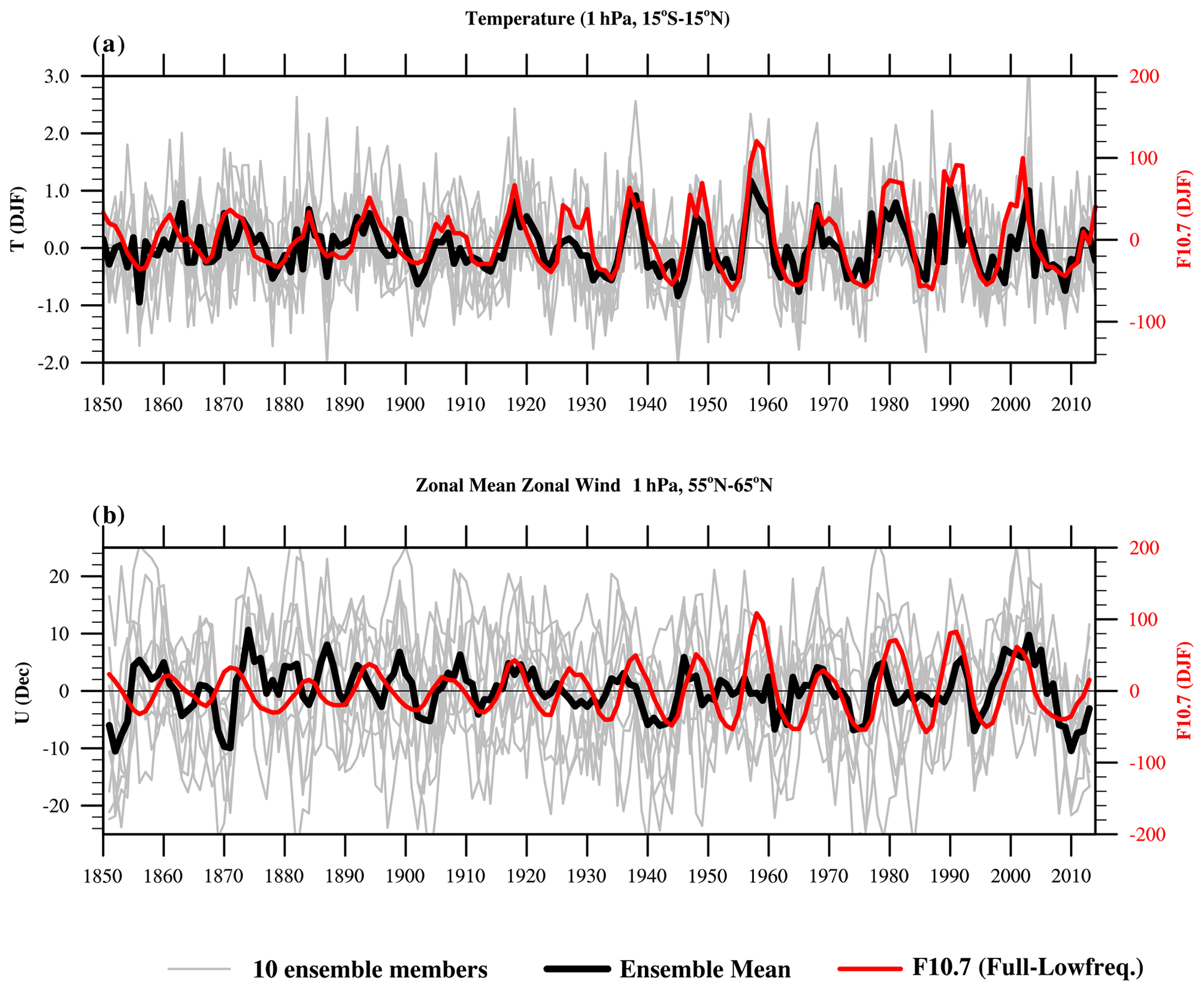
Figure 3Direct solar cycle signal in the upper stratosphere. (a) Time series of the tropical stratopause temperature (1 hPa, 15∘ S–15∘ N) averaged over the winter season (DJF) for the individual ensemble members (thin gray lines), ensemble mean (thick black line), and the solar cycle index F10.7 (red line). (b) Same as (a) but for December zonal mean zonal wind averaged over 55–65∘ N, 1 hPa, smoothed with a 3-year running mean. To isolate 11-year solar cycle effects, differences between the FULL and the LOWFREQ ensemble simulations have been calculated. The gray lines include internal variability and the 11-year solar signal, their spread represents the internal variability, and the ensemble mean (thick black line) represents the 11-year solar cycle signal. The 11-year solar cycle has been isolated in a similar way from the original solar forcing time series by subtracting the low-frequency part of the solar forcing (Fig. S1).
Consistent with the zonal mean zonal wind anomalies (Fig. S5) a clear and statistically significant surface response appears in sea level pressure (SLP) in February featuring higher-pressure anomalies in the midlatitudes and lower-pressure anomalies over the North Pole with a minimum over Scandinavia and the Norwegian Sea representing a negative Northern Annular Mode pattern during the strong epoch (Fig. 4a). Consistent with the annular SLP and wind signals a statistically significant response in sea surface temperatures (SSTs) in the North Atlantic appears (Fig. 4b). The model response is strongest at the time when the strongest zonal mean zonal wind signal extends down to the surface, propagating poleward and downward from the stratosphere (Fig. S5).
The solar signal in SLP resembles the tripolar NAO pattern (Visbeck et al., 2003), but it is shifted towards Europe with centers over Scandinavia and the Mediterranean Sea (and a secondary maximum towards North America) as compared to the NAO, which has action centers close to Iceland and the Azores (Fig. 4a). To further investigate the role of the solar cycle for decadal climate variability in the North Atlantic region, we focus on the NAO-like solar signal in the following.

Figure 4Solar surface signal in NH winter at lag 0 during the strong epoch. Composite differences between the solar maximum and minimum for (a) SLP (contours) and wind at 850 hPa (vectors) in February. Only those vectors where the zonal mean wind component is significant at the 90 % level are shown. The two green circles indicate the stations used for the NAO index calculation (see “Methods” section for more details). (b) Same as (a) but for SST (contours) averaged over the winter season (DJF). White dots indicate 90 % statistically significant regions based on a 1000-fold bootstrapping test.
The NAO-like mode (green markers in Fig. 4a; see “Methods” section) exhibits typical quasi-decadal internally generated oscillations during NH winter (see blue line in Fig. S8). The solar cycle synchronizes the phase of the NAO-like index in February during the strong epoch (Fig. 5a), while the internally generated decadal-scale NAO has no clear phase relationship with the solar cycle (Fig. 5b). The relationship between the solar cycle and the model ensemble mean NAO index is stable only during the strong epoch when the solar cycle forcing is strong. Their running correlation for all overlapping 45-year windows fluctuates in the earlier years but begins to rise in the 1920s both for the model (at 0 lag) and observations (first with a lag of 2 years, later 0 years) (Fig. 5c; cf. Fig. 7a in Kuroda et al., 2022, who also see a shift of the lag from +2 to 0 in observations around 1975 as shown here). In the second half of the 20th century, the correlations reach statistical significances of 90 % for the model NAO at 0 lag, while in observations significant correlations appear when the NAO lags behind the solar cycle by 2 years (Gray et al., 2013; Thiéblemont et al., 2015) and since the 1980s when there is no lag (see “Discussion”). A comparison of the solar signal in the NAO with internal NAO variability reveals that the solar signal in SLP over Europe is approximately 19 % the magnitude of internal variability during the strong epoch. This comparison is done by calculating the variances of the smoothed ensemble mean index and those of the smoothed individual members. The solar cycle signal is small in magnitude but manifests itself as an organization of the NAO as shown by the cross-correlations (Fig. 5a) and the increasing running correlations (Fig. 5c), which is in agreement with earlier studies (Otterå et al., 2010; Scaife et al., 2013; Thiéblemont et al., 2015). We show here that in our model this “organization” depends on the solar cycle amplitude, and it is large enough for a potential predictability variance fraction (ppvf) of up to 25 % in the North Atlantic region (Fig. 1a).
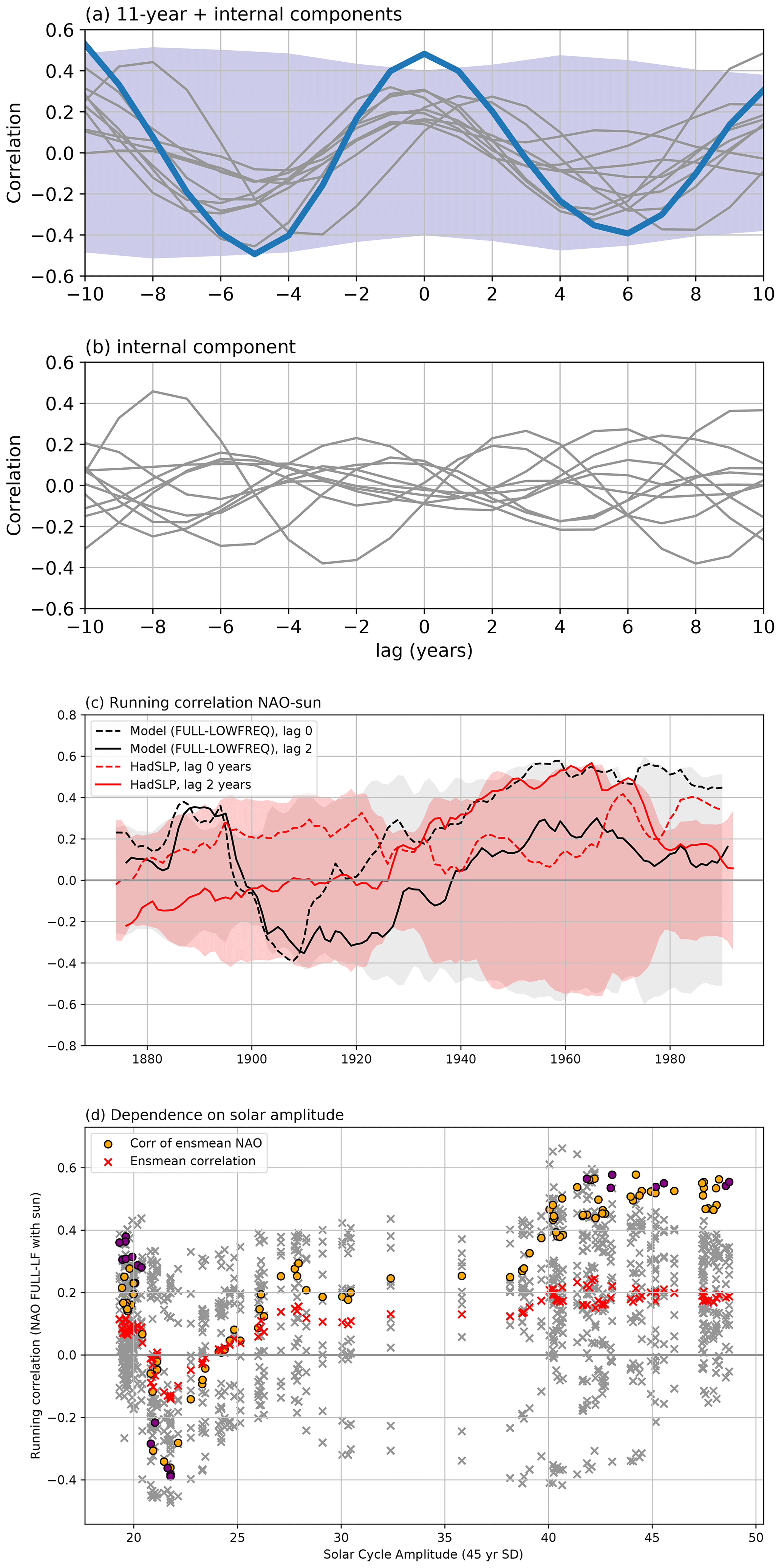
Figure 5Synchronization of internal variability modes in the Atlantic with the solar cycle. Cross-correlation between the wintertime (DJF) solar index (F10.7 solar flux) and the February NAO-like station-based indices for (a) 11-year + internal components (FULL minus ensemble mean of LOWFREQ) and (b) internal component (FULL minus ensemble mean of FULL) during the strong epoch (gray thin lines: individual members; blue line: ensemble mean). The 90 % significance level is shown as a shaded envelope (light blue). (c) The 45-year running correlation of NAO indices in February from the model (black lines; differences of the ensemble mean NAO indices as explained in the “Methods” section) and observation (red solid (lag 2 years) and red dashed (lag 0 years) lines) with the F10.7 index. The year on the x axis denotes the central year of the window (in the case of the lagged time series it is with respect to the NAO index). All indices are station-based and smoothed with a 3-year running mean prior to calculating the correlation. The 90 % significance level is shown as shaded envelopes, for model (gray) and observations (light red) separately. (d) Scatterplot of February NAO–Sun running correlations (FULL–LOWFREQ, smoothed with 3-year running mean, 45-year windows; similar to Fig. 5c) against solar cycle amplitude (standard deviation of smoothed F10.7 time series, same 45-year windows). Red crosses are the ensemble mean of correlations of single ensemble members with the solar index. Dots are the correlation of the ensemble mean NAO with the solar index; purple dots are correlations that exceed the 90 % significance level calculated with a random-phase test.
Note that the observations only provide one realization, which includes all external forcings as well as internal variability. We show that a significant solar signal in the North Atlantic region is generated by the 11-year solar cycle in our 10-member ensemble simulations during the strong epoch. The alignment of the surface pressure pattern with the solar cycle after the 1920s can also be seen nicely in the NAO-like time series (Fig. S8), which agrees with a number of earlier studies (Dima et al., 2005; Gray et al., 2016; Ma et al., 2018). A weak imprint can even be seen in the EOF-based NAO index (Fig. S8).
The dependence of the correlation strength on the solar cycle amplitude can be seen in Fig. 5d: while for low solar cycle amplitudes, correlations are scattered around zero, they are larger and positive for enhanced solar cycle amplitudes. Note that we do not expect larger correlations since the NAO index represents near-surface signals and as discussed above the solar surface signal is small. Even though correlations for observations as in Fig. 5c are similar to what has been shown in a recent study (see Fig. 1b in Chiodo et al., 2019), our conclusions are very different in the light of our model results.
Recent analyses of the solar influence on the North Atlantic revealed insignificant responses (Chiodo et al., 2019), whereas numerous previous studies have found statistically significant solar cycle signals in surface climate in observations and climate models (Gray et al., 2010, 2013, 2016; Kodera, 2003; Kodera et al., 2016; Matthes et al., 2006) and even proposed a synchronization of the NAO by the 11-year solar cycle through the “top–down” stratospheric mechanism (Thiéblemont et al., 2015). However, as we show here, the solar signal is likely not present in all winter months. Therefore, in some studies there remains a signal in DJF means, while it could be averaged out in others, including ours (see below). This finding is also supported by the very recent study of Kuroda et al. (2022).
Here, we systematically detected solar-induced atmospheric and surface signals and separated them from internal variability as well as other external forcings based on two 10-member ensembles. With this unique dataset, it was possible to overcome the problems in observations where a separation of solar-forced variability and a comparison to other external forcings and internal variability are impossible.
We demonstrate that in our model the strength of the solar surface signal depends on the amplitude of the solar cycle. A stronger signal is detected during the “strong solar cycle epoch” and explains the limited detectability of observed surface signals before the 1930s as well as discrepancies in earlier studies. We show that a stronger solar cycle signal induces a surface response that resembles the NAO, and the NAO-like index is organized by the solar cycle. This means the solar cycle enhances the probability of a specific decadal NAO phase if the solar forcing is strong enough. During solar maximum, there is a tendency for a positive decadal-scale NAO and vice versa. Our study confirms previous studies (Misios and Schmidt, 2012; Thiéblemont et al., 2015) which used the strong epoch for their solar forcing.
We find statistically significant ensemble mean solar-cycle-induced surface signals in February during the strong epoch which are consistent with the top–down propagation from stratospheric signals. This limitation of the solar signal to February is also confirmed by Kuroda et al. (2022) using long observational datasets as well as a historical simulation with a different chemistry–climate model. A controversial study (Chiodo et al., 2019) making use of a combined DJF surface pressure pattern could not detect significant surface signals in their SOL simulation (a simulation which includes the idealized 11-year solar cycle). Our results (see also Figs. S4–S5) suggest that it might be necessary to analyze monthly fields to capture the top–down propagation of the solar-induced wind anomalies and surface signals. Analyzing our model using DJF means, we only find a very weak signal in SLP and no significant zonal mean zonal wind signal in the lower troposphere during the strong epoch either (Figs. S11–S12). Also, although the base model is quite similar, there are a couple of important differences. Whereas we use two 10-member ensemble simulations of the historical period ( years = 2×1650 years; for the strong epoch this means: years) with the CMIP6 solar forcing (radiative and particle forcing) and the anthropogenic signal included, the other study uses two 500-year integrations with perpetual anthropogenic conditions representative of the year 2000 and an idealized solar forcing which repeats the last four solar cycles (cycle 20–23) and does not include the low-frequency component over the historical period. For the analysis of sea level pressure or zonal mean winds, relatively short 100- or 30-year periods are considered, whereas we have 10 members of 83 years each for the strong period. We isolate the 11-year solar cycle signal by subtracting the LOWFREQ ensemble mean from the FULL ensemble, whereas the other study compares the simulation which includes the idealized 11-year solar cycle (SOL) with a simulation that does not include any solar forcing (NOSOL). While we are careful to remove the influence of low-frequency solar variation by subtracting the LOWFREQ ensemble mean, we cannot be sure that a non-linear influence was properly excluded and hence can be compared to idealized solar forcing. It should also be noted that the model version used by Chiodo et al. (2019) simulates the top–down mechanism and a surface signal, even for DJF means, when using higher solar forcing (see their Supplement).
We would like to note that there are still some discrepancies between our simulations and observations, such as the different timing and location of maximum responses. We do not find a lagged NAO response in our simulations (cf., e.g., Gray et al., 2013), and the synchronization can only be found in February when the solar-induced zonal mean wind reaches the surface (cf. Kuroda et al., 2022), while the largest response in observations appears at a lag of 2 years since the 1940s and throughout the 1970s, and thereafter the lag vanishes (Kuroda et al., 2022) (see also Fig. S10 for the SLP signal in the strong epoch). Possible reasons for these discrepancies are (i) that the observational record is only one ensemble member that includes all internal variability and responses to all external forcings (which may even cause what appears as a lagged response, the lag itself being by chance), (ii) that the model feedback from the ocean is insufficient, and (iii) that the influence of the solar cycle is highly non-linear, which is very difficult to grasp.
The importance of the periodic solar cycle is particularly interesting for decadal climate predictions. Our results indicate that the solar cycle has a significant contribution to the potential predictability of up to 20 %–25 % in the North Atlantic during winter, where the climate response to external forcings such as greenhouse gases is comparably low. This offers the opportunity to increase decadal prediction skills in particular over Europe. This is in line with a very recent study which found exactly this region to be particularly sensitive to natural external forcings such as volcanic aerosols and solar activity when comparing decadal prediction systems from CMIP5 and CMIP6 (Borchert et al., 2021). Besides a sufficiently large ensemble (see Fig. S9), the key for climate models to exploit this potential originating in solar forcing is the incorporation of necessary prerequisites to simulate the effects of the solar cycle: a realistic, spectrally resolved solar forcing dataset, either interactive chemistry or at least an ozone forcing including an estimate of the solar cycle impact, and a well-resolved shortwave radiation scheme to account for the solar UV changes.
6.1 Model description
We use the fourth version of the Whole Atmosphere Community Climate Model (WACCM4) (Marsh et al., 2013), which is part of the Community Earth System Model suite (CESM) version 1.0.6 (Hurrell et al., 2013). CESM1(WACCM) is an extension of the Community Atmospheric Model (CAM4) (Kinnison et al., 2007; Neale et al., 2013). It covers the atmosphere from the surface to the lower thermosphere ( hPa; approx. 145 km) and is considered a high-top model. CESM1(WACCM) has a horizontal resolution of 1.9∘ × 2.5∘ and 66 vertical levels. It includes a middle-atmosphere chemistry module, which is based on the Model for Ozone and Related Chemical Tracers (MOZART3) (Garcia et al., 2014), comprising a total number of 59 species and 217 gas-phase chemical reactions (including all members of the Ox, NOx, and HOx chemical groups). For the presented simulations, we implemented a set of model improvements (Garcia et al., 2014, 2017; Smith et al., 2014). These include an increased turbulent Prandtl number yielding an increased diffusion coefficient as well as modifications related to gravity waves: (i) the orographic gravity wave drag does not depend on the land fraction of the grid box anymore, and (ii) the ratio of energy from dissipating gravity waves that is transformed into heat has been reduced to 30 %. Since this model version is not able to internally generate a quasi-biennial oscillation (QBO), we relax stratospheric equatorial winds towards an idealized QBO with a fixed 28-month period (Matthes et al., 2010). The POP ocean module has a tripolar horizontal grid of 1∘ × 1∘ and 60 depth levels.
6.2 Experimental design
The two 10-member ensemble simulations, FULL and LOWFREQ, cover 165 years each from 1850 through 2014, follow the CMIP5 historical recommendations for all external forcings from 1850–2004, and continue with the RCP4.5 scenario afterwards. Only for the solar forcing has the improved CMIP6 dataset been used (Matthes et al., 2017). The FULL ensemble experiences the complete solar variability from the CMIP6 dataset with total and spectrally resolved solar irradiances as well as auroral electron effects. Higher-energy electrons are not considered in this study; however, a recent study suggests that these are not of substantial relevance for the solar signal in the NAO (Guttu et al., 2021). The LOWFREQ ensemble only includes the low-frequency part of solar variability by low-pass filtering the solar forcing with a 33-year running mean (Fig. S1). The individual ensemble members of FULL and LOWFREQ have been each initialized from different climate states of a multi-centennial pre-industrial control simulation.
6.3 Observations
The NOAA Global Surface Temperature (NOAAGlobalTemp V4.0.1) including The Extended Reconstructed Sea Surface Temperature (ERSST) dataset (version 5) (Huang et al., 2017) and land surface air temperature data from the Global Historical Climatology Network Monthly dataset (Menne et al., 2018) is used to calculate correlations with the model simulations. HadSLP2r data (Allan and Ansell, 2006) are used to calculate the observed NAO index as well as composites. All these data are provided by the NOAA/OAR/ESRL PSL, Boulder, Colorado, USA, from their websites at https://psl.noaa.gov/data/gridded/data.noaaglobaltemp.html and https://psl.noaa.gov/gcos_wgsp/Gridded/data.hadslp2.html (last access: 19 September 2019).
6.4 Disentangling internal and external variability
The single members in one ensemble (FULL or LOWFREQ) share the same externally forced signals but have different internal variability. To isolate the internal variability from external forcings, the ensemble average of the respective ensemble (FULL or LOWFREQ) has to be subtracted from the individual members. The ensemble mean (average over all individual members) represents the combined effects of all external forcings. External forcings in the LOWFREQ ensemble comprise low-frequency solar variability as well as changes in greenhouse gases, while in the FULL ensemble additionally the effect of the 11-year solar cycle is included. In order to isolate the solar cycle from other external forcings, the ensemble mean of the LOWFREQ ensemble has to be subtracted from the ensemble mean of the FULL ensemble.
6.5 Definition of weak epoch and strong epoch
Two periods (weak and strong epoch) with different solar cycle amplitudes were analyzed separately. Considering the continuous integration to capture the climate evolution with changing solar and anthropogenic forcing similar to observations, we defined the weak epoch from 1850 to 1931 and the strong epoch from 1932 to 2014. It is important to note that each epoch includes seven entire solar cycles but with different solar cycle amplitudes. The solar cycle amplitudes in the weak and strong epochs defined by the difference between the smoothed F10.7 maximum and minimum (red and blue dots in Fig. S1) of each cycle are shown in Table S1, as well as the standard deviation of the smoothed F10.7 in each cycle. A different sorting of the weak and strong solar cycle amplitudes was tested since cycle 15 is stronger than others in the weak epoch and cycle 20 is weaker than others in the strong epoch, but it was rejected since only one solar cycle (cycle 15) in the weak epoch showed slightly enhanced amplitude and it was checked that this does not affect our results.
6.6 Decadal potential predictability
The potential predictability variance fraction (ppvf) (Boer, 2004) is used to quantify the fraction of the decadal variability (8-year running mean) (i) forced by the 11-year solar cycle, (ii) forced by all other external forcings (including the low-frequency component of solar variability), and (iii) due to internal variability. First, we calculate the variance of each of these components (disentangling solar cycle and external and internal components as described above) and then divide it by the total variance to obtain the ppvf of each component. An 8-year running mean was applied to surface temperatures before calculating the variance in order to isolate decadal variability. Other window lengths between 7 and 10 years were tested to exclude sensitivity of the results to the averaging period; the results were very similar for all window lengths. Statistically insignificant regions (p>0.05) in Fig. 1a and b are estimated by analyzing the ppvf attributed to the solar cycle and the low-frequency external components in comparison to the internal variance fractions by means of a Fisher's f test in line with earlier studies (Boer, 2004). Calculations in Fig. 1a take into account the reduction of effective sample size due to the application of a low-pass filter.
6.7 Composites, correlations, and statistical significances
Solar cycle-based composites are used to identify solar signals. The monthly time series of the F10.7 radio flux in solar flux units (1 sfu = 10−22 W m−2 Hz−1) is smoothed with a 3-year running mean (orange line) to determine local solar maxima and minima in January as representative of boreal winter (Fig. S1). Three years around each maximum and minimum are selected (dots in Fig. S1). Solar composites are then calculated as differences between averages of all solar maximum years and all solar minimum years. A 1000-fold bootstrapping test with replacement (Diaconis and Efron, 1983) is used to estimate the 90 % statistical significances of the ensemble mean composites compared to the individual ensemble members. Cross-correlations and running correlations are calculated with a 45-year window to investigate the relationship between the 11-year solar cycle forced signal and natural internal decadal variability. The significance test for correlations was calculated based on 10 000 random time series with random phases (Ebisuzaki, 1997).
6.8 NAO index definition
The model NAO-like index was created by selecting locations close to the centers of the minimum and maximum of the solar-induced SLP composites in February (Fig. 4a, green markers, 65.37∘ N, 22.5∘ E and 38.84∘ N, 17.5∘ E). Note that this NAO definition is comparable to a landmark study (Exner, 1913) which described the spatial structure of the NAO first (Hurrell and Deser, 2015). For observations, the HadSLP2r dataset was used with stations in Reykjavík, Iceland, and Lisbon, Portugal. First the February SLP at each location was normalized (all-time mean subtracted and then divided by the standard deviation over the time series) and then the difference between the northern and the southern stations was calculated. For the model data, this was done for every member in the FULL and LOWFREQ ensemble, before calculating the two ensemble means. Finally, the LOWFREQ ensemble mean was subtracted from the FULL ensemble mean, to investigate the effects of the solar cycle only. The running correlations in Fig. 5c were calculated by (i) applying a 3-year running mean to the NAO-like time series and the F10.7 time series of DJF averages and (ii) choosing the same 45-year windows for both time series (or shifted by 2 years for the lagged correlations) and correlating them, moving forward 1 year at a time. The year on the x axis denotes the central year of the 45-year NAO-like time series window.
The source code of the Community Earth System Model version 1.0 (CESM 1.0.6) used in this study is publicly distributed and can be obtained after registration at http://www.cesm.ucar.edu/models/cesm1.0/ (CESM, 2020). Codes to reproduce the analysis and figures are archived at Zenodo (https://doi.org/10.5281/zenodo.6619200, Drews et al., 2022) and are available from the corresponding author upon reasonable request.
All raw model output is available from the CERA long-term archive at DKRZ (solar full: http://cera-www.dkrz.de/WDCC/ui/Compact.jsp?acronym=DKRZ_LTA_519_ds00036, Kruschke et al. (2020a); solar lowfreq: http://cera-www.dkrz.de/WDCC/ui/Compact.jsp?acronym=DKRZ_LTA_519_ds00035, Kruschke et al. (2020b)). Post-processed datasets (observational and model) are available from the corresponding author upon reasonable request.
The supplement related to this article is available online at: https://doi.org/10.5194/acp-22-7893-2022-supplement.
AD did the analysis and produced Figs. 2 and 5 as well as S1 and S8 in the Supplement, WH did the analysis and produced Figs. 3 and 4, S3–S7, and S9–S13 in the Supplement. TK produced Figs. 1 and S2, all in correspondence with KM, who initiated the study. TK initiated and performed the model simulations. KK assisted with the interpretation of the results. AD wrote the final version of the paper with input from all co-authors.
The contact author has declared that neither they nor their co-authors have any competing interests.
Publisher’s note: Copernicus Publications remains neutral with regard to jurisdictional claims in published maps and institutional affiliations.
We would like to thank a number of colleagues for continuous discussions about the solar influence on climate during the last years, in particular Bernd Funke as well as Lesley Gray, Joanna Haigh, Adam Scaife, and Hauke Schmidt. We are grateful for continued computing support and resources provided by the Deutsche Klimarechenzentrum (DKRZ) in Hamburg, Germany, where all simulations were performed. We thank Joakim Kjellsson for help with downloading the CMIP5 high-top model data. This work has been conducted within the framework of the WCRP/SPARC SOLARIS-HEPPA activity. We thank all the scientists, software engineers, and administrators who contributed to the development of CESM.
This research has been funded by the Federal Ministry of Education and Research in Germany (ROMIC-SOLIC project (grant no. 01LG1219)) and the European Union under Horizon 2020 (EUCP project (grant no. 776613)).
The article processing charges for this open-access publication were covered by the GEOMAR Helmholtz Centre for Ocean Research Kiel.
This paper was edited by Patrick Jöckel and reviewed by two anonymous referees.
Allan, R. and Ansell, T.: A New Globally Complete Monthly Historical Gridded Mean Sea Level Pressure Dataset (HadSLP2): 1850–2004, J. Climate, 19, 5816–5842, https://doi.org/10.1175/JCLI3937.1, 2006.
Andrews, M. B., Knight, J. R., and Gray, L. J.: A simulated lagged response of the North Atlantic Oscillation to the solar cycle over the period 1960–2009, Environ. Res. Lett., 10, 054022, https://doi.org/10.1088/1748-9326/10/5/054022, 2015.
Bellucci, A., Haarsma, R., Gualdi, S., Athanasiadis, P. J., Caian, M., Cassou, C., Fernandez, E., Germe, A., Jungclaus, J., Kröger, J., Matei, D., Müller, W., Pohlmann, H., Salas y Melia, D., Sanchez, E., Smith, D., Terray, L., Wyser, K., and Yang, S.: An assessment of a multi-model ensemble of decadal climate predictions, Clim. Dynam., 44, 2787–2806, https://doi.org/10.1007/s00382-014-2164-y, 2015.
Boer, G. J.: Long time-scale potential predictability in an ensemble of coupled climate models, Clim. Dynam., 23, 29–44, https://doi.org/10.1007/s00382-004-0419-8, 2004.
Boer, G. J., Kharin, V. V., and Merryfield, W. J.: Decadal predictability and forecast skill, Clim. Dynam., 41, 1817–1833, https://doi.org/10.1007/s00382-013-1705-0, 2013.
Borchert, L. F., Menary, M. B., Swingedouw, D., Sgubin, G., Hermanson, L., and Mignot, J.: Improved Decadal Predictions of North Atlantic Subpolar Gyre SST in CMIP6, Geophys. Res. Lett., 48, e2020GL091307, https://doi.org/10.1029/2020GL091307, 2021.
CESM (Community Earth System Model): Software Engineering Group (CESG), NCAR: CESM1.0 Public Release [code], http://www.cesm.ucar.edu/models/cesm1.0 (last access: 30 May 2022), 2020.
Chiodo, G., Oehrlein, J., Polvani, L. M., Fyfe, J. C., and Smith, A. K.: Insignificant influence of the 11-year solar cycle on the North Atlantic Oscillation, Nat. Geosci., 12, 94–99, https://doi.org/10.1038/s41561-018-0293-3, 2019.
Diaconis, P. and Efron, B.: Computer-intensive methods in statistics, Sci. Am., 248, 116–131, https://doi.org/10.1038/scientificamerican0583-116, 1983.
Dima, M., Lohmann, G., and Dima, I.: Solar-induced and internal climate variability at decadal time scales, Int. J. Climatol., 25, 713–733, https://doi.org/10.1002/joc.1156, 2005.
Drews, A., Huo, W., Matthes, K., Kodera, K., and Wahl, S.: acp-2021-241, in ACP (1.0), Zenodo [code], https://doi.org/10.5281/zenodo.6619200, 2022.
Dunstone, N., Smith, D., Scaife, A., Hermanson, L., Eade, R., Robinson, N., Andrews, M., and Knight, J.: Skilful predictions of the winter North Atlantic Oscillation one year ahead, Nat. Geosci., 9, 809–814, https://doi.org/10.1038/ngeo2824, 2016.
Ebisuzaki, W.: A Method to Estimate the Statistical Significance of a Correlation When the Data Are Serially Correlated, J. Climate, 10, 2147–2153, https://doi.org/10.1175/1520-0442(1997)010<2147:AMTETS>2.0.CO;2, 1997.
Exner, F. M.: Über monatliche Witterungsanomalien auf der nördlichen Erdhälfte im Winter, Hölder, 1913.
Garcia, R. R., López-Puertas, M., Funke, B., Marsh, D. R., Kinnison, D. E., Smith, A. K., and González-Galindo, F.: On the distribution of CO2 and CO in the mesosphere and lower thermosphere, J. Geophys. Res.-Atmos., 119, 5700–5718, https://doi.org/10.1002/2013JD021208, 2014.
Garcia, R. R., Smith, A. K., Kinnison, D. E., de la Cámara, Á., and Murphy, D. J.: Modification of the Gravity Wave Parameterization in the Whole Atmosphere Community Climate Model: Motivation and Results, J. Atmos. Sci., 74, 275–291, https://doi.org/10.1175/JAS-D-16-0104.1, 2017.
Goddard, L., Kumar, A., Solomon, A., Smith, D., Boer, G., Gonzalez, P., Kharin, V., Merryfield, W., Deser, C., Mason, S. J., Kirtman, B. P., Msadek, R., Sutton, R., Hawkins, E., Fricker, T., Hegerl, G., Ferro, C. A. T., Stephenson, D. B., Meehl, G. A., Stockdale, T., Burgman, R., Greene, A. M., Kushnir, Y., Newman, M., Carton, J., Fukumori, I., and Delworth, T.: A verification framework for interannual-to-decadal predictions experiments, Clim. Dynam., 40, 245–272, https://doi.org/10.1007/s00382-012-1481-2, 2013.
Gray, L. J., Beer, J., Geller, M., Haigh, J. D., Lockwood, M., Matthes, K., Cubasch, U., Fleitmann, D., Harrison, G., Hood, L., Luterbacher, J., Meehl, G. A., Shindell, D., van Geel, B., and White, W.: Solar Influences on Climate, Rev. Geophys., 48, RG4001, https://doi.org/10.1029/2009RG000282, 2010.
Gray, L. J., Scaife, A. A., Mitchell, D. M., Osprey, S., Ineson, S., Hardiman, S., Butchart, N., Knight, J., Sutton, R., and Kodera, K.: A lagged response to the 11 year solar cycle in observed winter Atlantic/European weather patterns, J. Geophys. Res.-Atmos., 118, 2013JD020062, https://doi.org/10.1002/2013JD020062, 2013.
Gray, L. J., Woollings, T. J., Andrews, M., and Knight, J.: Eleven-year solar cycle signal in the NAO and Atlantic/European blocking, Q. J. Roy. Meteor. Soc., 142, 1890–1903, https://doi.org/10.1002/qj.2782, 2016.
Guttu, S., Orsolini, Y., Stordal, F., Otterå, O. H., Omrani, N.-E., Tartaglione, N., Verronen, P. T., Rodger, C. J., and Clilverd, M. A.: Impacts of UV Irradiance and Medium-Energy Electron Precipitation on the North Atlantic Oscillation during the 11-Year Solar Cycle, Atmosphere, 12, 1029, https://doi.org/10.3390/atmos12081029, 2021.
Haigh, J. D.: The role of stratospheric ozone in modulating the solar radiative forcing of climate, Nature, 370, 544–546, https://doi.org/10.1038/370544a0, 1994.
Huang, B., Thorne, P. W., Banzon, V. F., Boyer, T., Chepurin, G., Lawrimore, J. H., Menne, M. J., Smith, T. M., Vose, R. S., and Zhang, H.-M.: Extended Reconstructed Sea Surface Temperature, Version 5 (ERSSTv5): Upgrades, Validations, and Intercomparisons, J. Climate, 30, 8179–8205, https://doi.org/10.1175/JCLI-D-16-0836.1, 2017.
Hurrell, J. W. and Deser, C.: Northern Hemisphere climate variability during winter: Looking back on the work of Felix Exner, Meteorol. Z., 24, 113–118, https://doi.org/10.1127/metz/2015/0578, 2015.
Hurrell, J. W., Holland, M. M., Gent, P. R., Ghan, S., Kay, J. E., Kushner, P. J., Lamarque, J.-F., Large, W. G., Lawrence, D., Lindsay, K., Lipscomb, W. H., Long, M. C., Mahowald, N., Marsh, D. R., Neale, R. B., Rasch, P., Vavrus, S., Vertenstein, M., Bader, D., Collins, W. D., Hack, J. J., Kiehl, J., and Marshall, S.: The Community Earth System Model: A Framework for Collaborative Research, B. Am. Meteorol. Soc., 94, 1339–1360, https://doi.org/10.1175/BAMS-D-12-00121.1, 2013.
Kinnison, D. E., Brasseur, G. P., Walters, S., Garcia, R. R., Marsh, D. R., Sassi, F., Harvey, V. L., Randall, C. E., Emmons, L., Lamarque, J. F., Hess, P., Orlando, J. J., Tie, X. X., Randel, W., Pan, L. L., Gettelman, A., Granier, C., Diehl, T., Niemeier, U., and Simmons, A. J.: Sensitivity of chemical tracers to meteorological parameters in the MOZART-3 chemical transport model, J. Geophys. Res.-Atmos., 112, D20302, https://doi.org/10.1029/2006JD007879, 2007.
Kodera, K.: Solar influence on the spatial structure of the NAO during the winter 1900–1999, Geophys. Res. Lett., 30, 1175, https://doi.org/10.1029/2002GL016584, 2003.
Kodera, K. and Kuroda, Y.: Dynamical response to the solar cycle, J. Geophys. Res.-Atmos., 107, ACL 5-1–ACL 5-12, https://doi.org/10.1029/2002JD002224, 2002.
Kodera, K., Thiéblemont, R., Yukimoto, S., and Matthes, K.: How can we understand the global distribution of the solar cycle signal on the Earth's surface?, Atmos. Chem. Phys., 16, 12925–12944, https://doi.org/10.5194/acp-16-12925-2016, 2016.
Kruschke, T., Matthes, K., and Wahl, S.: CESM1.0.6 full solar variability ensemble, DOKU at DKRZ [data set] , http://cera-www.dkrz.de/WDCC/ui/Compact.jsp?acronym=DKRZ_LTA_519_ds00036 (last access: 7 June 2022), 2020a.
Kruschke, T., Matthes, K., and Wahl, S.: CESM1.0.6 low frequency solar variability ensemble, DOKU at DKRZ [data set], http://cera-www.dkrz.de/WDCC/ui/Compact.jsp?acronym=DKRZ_LTA_519_ds00035 (last access: 7 June 2022), 2020b.
Kuroda, Y., Kodera, K., Yoshida, K., Yukimoto, S., and Gray, L.: Influence of the solar cycle on the North Atlantic Oscillation, J. Geophys. Res.-Atmos., 127, e2021JD035519, https://doi.org/10.1029/2021JD035519, 2022.
Kushnir, Y., Scaife, A. A., Arritt, R., Balsamo, G., Boer, G., Doblas-Reyes, F., Hawkins, E., Kimoto, M., Kolli, R. K., Kumar, A., Matei, D., Matthes, K., Müller, W. A., O'Kane, T., Perlwitz, J., Power, S., Raphael, M., Shimpo, A., Smith, D., Tuma, M., and Wu, B.: Towards operational predictions of the near-term climate, Nat. Clim. Change, 9, 94–101, https://doi.org/10.1038/s41558-018-0359-7, 2019.
Ma, H., Chen, H., Gray, L., Zhou, L., Li, X., Wang, R., and Zhu, S.: Changing response of the North Atlantic/European winter climate to the 11 year solar cycle, Environ. Res. Lett., 13, 034007, https://doi.org/10.1088/1748-9326/aa9e94, 2018.
Marsh, D. R., Mills, M. J., Kinnison, D. E., Lamarque, J.-F., Calvo, N., and Polvani, L. M.: Climate Change from 1850 to 2005 Simulated in CESM1 (WACCM), J. Climate, 26, 7372–7391, https://doi.org/10.1175/JCLI-D-12-00558.1, 2013.
Matthes, K., Kuroda, Y., Kodera, K., and Langematz, U.: Transfer of the solar signal from the stratosphere to the troposphere: Northern winter, J. Geophys. Res.-Atmos., 111, D06108, https://doi.org/10.1029/2005JD006283, 2006.
Matthes, K., Marsh, D. R., Garcia, R. R., Kinnison, D. E., Sassi, F., and Walters, S.: Role of the QBO in modulating the influence of the 11 year solar cycle on the atmosphere using constant forcings, J. Geophys. Res.-Atmos., 115, D18110, https://doi.org/10.1029/2009JD013020, 2010.
Matthes, K., Funke, B., Andersson, M. E., Barnard, L., Beer, J., Charbonneau, P., Clilverd, M. A., Dudok de Wit, T., Haberreiter, M., Hendry, A., Jackman, C. H., Kretzschmar, M., Kruschke, T., Kunze, M., Langematz, U., Marsh, D. R., Maycock, A. C., Misios, S., Rodger, C. J., Scaife, A. A., Seppälä, A., Shangguan, M., Sinnhuber, M., Tourpali, K., Usoskin, I., van de Kamp, M., Verronen, P. T., and Versick, S.: Solar forcing for CMIP6 (v3.2), Geosci. Model Dev., 10, 2247–2302, https://doi.org/10.5194/gmd-10-2247-2017, 2017.
Menne, M. J., Williams, C. N., Gleason, B. E., Rennie, J. J., and Lawrimore, J. H.: The Global Historical Climatology Network Monthly Temperature Dataset, Version 4, J. Climate, 31, 9835–9854, https://doi.org/10.1175/JCLI-D-18-0094.1, 2018.
Misios, S. and Schmidt, H.: Mechanisms Involved in the Amplification of the 11-yr Solar Cycle Signal in the Tropical Pacific Ocean, J. Climate, 25, 5102–5118, https://doi.org/10.1175/JCLI-D-11-00261.1, 2012.
Neale, R. B., Richter, J., Park, S., Lauritzen, P. H., Vavrus, S. J., Rasch, P. J., and Zhang, M.: The Mean Climate of the Community Atmosphere Model (CAM4) in Forced SST and Fully Coupled Experiments, J. Climate, 26, 5150–5168, https://doi.org/10.1175/JCLI-D-12-00236.1, 2013.
Otterå, O. H., Bentsen, M., Drange, H., and Suo, L.: External forcing as a metronome for Atlantic multidecadal variability, Nat. Geosci., 3, 688–694, https://doi.org/10.1038/ngeo955, 2010.
Scaife, A. A., Ineson, S., Knight, J. R., Gray, L., Kodera, K., and Smith, D. M.: A mechanism for lagged North Atlantic climate response to solar variability, Geophys. Res. Lett., 40, 434–439, https://doi.org/10.1002/grl.50099, 2013.
Smith, A. K., López-Puertas, M., Funke, B., García-Comas, M., Mlynczak, M. G., and Holt, L. A.: Nighttime ozone variability in the high latitude winter mesosphere, J. Geophys. Res.-Atmos., 119, 13547–13564, https://doi.org/10.1002/2014JD021987, 2014.
Smith, D. M., Eade, R., Scaife, A. A., Caron, L.-P., Danabasoglu, G., DelSole, T. M., Delworth, T., Doblas-Reyes, F. J., Dunstone, N. J., Hermanson, L., Kharin, V., Kimoto, M., Merryfield, W. J., Mochizuki, T., Müller, W. A., Pohlmann, H., Yeager, S., and Yang, X.: Robust skill of decadal climate predictions, npj Climate and Atmospheric Science, 2, 1–10, https://doi.org/10.1038/s41612-019-0071-y, 2019.
Thiéblemont, R., Matthes, K., Omrani, N.-E., Kodera, K., and Hansen, F.: Solar forcing synchronizes decadal North Atlantic climate variability, Nat. Commun., 6, 8268, https://doi.org/10.1038/ncomms9268, 2015.
Visbeck, M., Chassignet, E. P., Curry, R. G., Delworth, T. L., Dickson, R. R., and Krahmann, G.: The Ocean's Response to North Atlantic Oscillation Variability, in: The North Atlantic Oscillation: Climatic Significance and Environmental Impact, edited by: Hurrell, J. W., Kushnir, Y., Ottersen, G., and Visbeck, M., 113–145, American Geophysical Union, https://doi.org/10.1029/134GM06, 2003.
Yeager, S. G. and Robson, J. I.: Recent Progress in Understanding and Predicting Atlantic Decadal Climate Variability, Curr. Clim. Change Rep., 3, 112–127, https://doi.org/10.1007/s40641-017-0064-z, 2017.
- Abstract
- Introduction
- Potential predictability associated with the solar cycle
- The top–down mechanism depends on solar cycle amplitude
- Solar-induced surface signals and synchronization of the NAO with the solar cycle
- Discussion
- Methods
- Code availability
- Data availability
- Author contributions
- Competing interests
- Disclaimer
- Acknowledgements
- Financial support
- Review statement
- References
- Supplement