The roles of the Quasi-Biennial Oscillation and El Niño for entry stratospheric water vapor in observations and coupled chemistry–ocean CCMI and CMIP6 models

The relative importance of two processes that help control the concentrations of stratospheric water vapor, the Quasi-Biennial Oscillation (QBO) and El Niño–Southern Oscillation (ENSO), are evaluated in observations and in comprehensive coupled ocean–atmosphere-chemistry models. The possibility of nonlinear interactions between these two is evaluated both using multiple linear regression (MLR) and three additional advanced machine learning techniques. The QBO is found to be more important than ENSO; however nonlinear interactions are nonnegligible, and even when ENSO, the QBO, and potential nonlinearities are included, the fraction of entry water vapor variability explained is still substantially less than what is accounted for by cold-point temperatures. While the advanced machine learning techniques perform better than an MLR in which nonlinearities are suppressed, adding nonlinear predictors to the MLR mostly closes the gap in performance with the advanced machine learning techniques. Comprehensive models suffer from too weak a connection between entry water and the QBO; however a notable improvement is found relative to previous generations of comprehensive models. Models with a stronger QBO in the lower stratosphere systematically simulate a more realistic connection with entry water.

1 Introduction

Water vapor (WV) provides most of the greenhouse effect in the atmosphere and of the total water vapor feedback to increasing anthropogenic greenhouse gas emissions; roughly 10 % is associated with water vapor in the stratosphere (Forster and Shine, 1999; Solomon et al., 2010; Dessler et al., 2013; Wang et al., 2017; Banerjee et al., 2019). The amount of water vapor that enters the stratosphere is also important for stratospheric chemistry and specifically the severity of ozone depletion (Solomon, 1999; Dvortsov and Solomon, 2001; Stenke and Grewe, 2005; Tian et al., 2009; Drdla and Müller, 2012; Robrecht et al., 2021). Hence, it is important to understand the factors that control the entry of water vapor into the stratosphere on all timescales and to consider whether comprehensive models used for ozone and climate change assessments represent these factors correctly.

Most of the water vapor in the lower stratosphere transited from the tropical upper troposphere through the tropical tropopause, and therefore tropical temperatures near the cold point largely determine lower stratospheric water vapor concentrations (Mote et al., 1996a; Zhou et al., 2004, 2001; Fueglistaler and Haynes, 2005a; Fueglistaler et al., 2009; Randel and Park, 2019). Many processes have been shown to modulate these cold-point temperatures, and the goal of this work is to re-evaluate the influence of these processes, and in particular their nonlinear interactions, on entry water vapor. We then consider the ability of comprehensive models to represent this effect.

The Quasi-Biennial Oscillation (QBO) modulates water vapor mixing ratios in air entering the stratosphere through its influence on temperatures in the tropical tropopause region (Reid and Gage, 1985; Zhou et al., 2001; Niwano et al., 2003; Zhou et al., 2004; Fujiwara et al., 2010; Liang et al., 2011; Kawatani et al., 2014; Diallo et al., 2018). Specifically, warmer cold-point temperatures during the QBO phase with westerlies near 50 hPa (hereafter wQBO) lead to moistening, and colder temperatures during the QBO phase with easterlies near 50 hPa (hereafter eQBO) lead to drying of the stratosphere. Comprehensive climate models typically struggle to capture the downward propagation of the QBO to the lower stratosphere (Rao et al., 2020a; Richter et al., 2020), and consistent with this, Smalley et al. (2017) found that the Chemistry Climate Model Validation Activity 2 (CCMVal2) models and most of the Chemistry-Climate Model Initiative (CCMI; Morgenstern et al., 2017) models they considered struggle to capture an influence of the QBO on entry water.

El Niño (EN), the El Niño–Southern Oscillation (ENSO) phase with anomalous warming of the tropical eastern Pacific, has been shown to lead to a cooler tropical lower stratosphere and warmer tropical troposphere (Free and Seidel, 2009; Randel et al., 2009; Calvo et al., 2010; Simpson et al., 2011). In addition, EN also forces a Rossby wave response that extends to the tropopause, whereby anomalously cold temperatures are present over the central Pacific, and anomalously warm temperatures are present over the Indo-Pacific warm pool (Yulaeva and Wallace, 1994; Randel et al., 2000; Zhou et al., 2001; Scherllin-Pirscher et al., 2012; Domeisen et al., 2019). This zonal dipole in temperature has been shown to affect water vapor below the cold point: water vapor decreases in the region with cold anomalies and increases in the region with warm anomalies by ∼25 % (Gettelman et al., 2001; Hatsushika and Yamazaki, 2003; Konopka et al., 2016).

The net effect of these temperature anomalies on tropical lower stratospheric water vapor is complex. While the lower stratosphere clearly was moister following the two largest EN events in the satellite era (in 1997/1998 and in 2015/2016) (Fueglistaler and Haynes, 2005a; Avery et al., 2017), moistening also was evident following two of the strongest La Niña events (in 1998/1999 and 1999/2000). The impact of more moderate events is less clear, and any net effect is not statistically significant considering the shortness of the data record (Garfinkel et al., 2018, 2021). Both La Niña and El Niño can lead to a moistening if the cold point moves zonally within the tropics (to the central Pacific for El Niño and to the far western Pacific for La Niña), and even though the lower stratospheric temperature response is opposite for El Niño and La Niña, the cold point appears to have warmed for both strong El Niño and strong La Niña events, explaining the moistening in 1997/1998, 1998/1999, 1999/2000 and 2015/2016 (Garfinkel et al., 2018). There is no consensus among models as to the sign of the impact of ENSO on water vapor, with many models predicting a response opposite to that observed (Garfinkel et al., 2021).

Finally, the strength of the Brewer–Dobson circulation (BDC) has been found to be important in determining entry water vapor, with a faster circulation associated with cooling of the cold point and dehydration (Randel et al., 2006; Dessler et al., 2013, 2014; Ye et al., 2018).

The net response to these various forcings is often quantified using multiple linear regression (e.g., Dessler et al., 2013; Smalley et al., 2017), which implicitly assumes that the response to these forcings is linear, i.e., that the response to a given magnitude El Niño is equal and opposite to that of a La Niña event of equal magnitude. This technique also assumes that the response to, e.g., ENSO and QBO, is the sum of the linear responses to each individual forcing (Diallo et al., 2018; Brinkop et al., 2016). Recent work has pointed out two faults of such an assumption. First, Garfinkel et al. (2018) and Garfinkel et al. (2021) found that the response to ENSO is nonlinear in observations (and also in some models), and hence such a methodology may underestimate the impact of ENSO on stratospheric water vapor. Second, Yuan et al. (2014) found that the QBO has a larger amplitude and a longer period during La Niña conditions than during El Niño. Hence the difference between the warmer cold-point temperatures (CPTs) during wQBO and colder CPTs during eQBO is larger during La Niña than during El Niño. This strengthens earlier findings that the greatest dehydration of air entering the stratosphere from the troposphere occurs during the winter under La Niña and easterly QBO conditions (Zhou et al., 2004; Liang et al., 2011). Specifically, Yuan et al. (2014) argue that the net effect of ENSO and the QBO is not just a linear superposition of their independent influences but the net result of their mutual interaction.

The goal of this work is to reconsider the relative importance of the QBO and ENSO while taking into consideration the possibility for nonlinearity in the response and to then consider whether the most recent comprehensive models are capable of simulating the response. After introducing the data and methodology in Sect. 2, we evaluate the relative successes of a multiple linear regression (MLR) and of more advanced machine learning (ML) techniques with ENSO, QBO, BDC, and mid-tropospheric temperature as predictors, in an attempt to find the factors that most succinctly explain observed interannual water vapor variability. We also consider the fraction of interannual entry water vapor variability that can be accounted for by variations of the cold-point temperature as an upper bound on how much water vapor variability is predictable from large-scale processes. We then add two nonlinear predictors to the MLR and demonstrate that they are as important as, e.g., a linear ENSO predictor. Finally, we consider the ability of comprehensive coupled ocean–atmosphere-chemistry models to simulate the connection between the QBO and entry water.

2 Data and methodology

2.1  Data

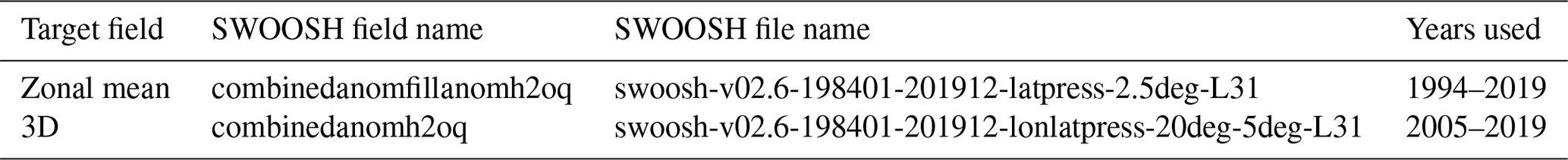
The Stratospheric Water and OzOne Satellite Homogenized data set (SWOOSH) (Davis et al., 2016) features a merged, gridded, homogenized and filled water vapor product from various limb sounding and solar occultation satellites over the previous ∼30 years. The measurements are monthly means comprised of the following instruments: SAGE-II/III, UARS HALOE, UARS MLS and Aura MLS. We use the zonal mean product (latitude, pressure) and the 3D (latitude, longitude, pressure) product as described in Table 1. The former has a high latitudinal resolution of 2.5^∘ and extends to the HALOE period (1990s), while the latter has a horizontal resolution of $\mathrm{20}{}^{\circ }\times \mathrm{5}{}^{\circ }$ but relies on the high sampling rates available with AURA MLS since 2004. While the latter data set does include some data as early as 1994, there are many gaps, and filling these gaps in a self-consistent way is out of the scope of this analysis. Both data sets have a pressure level range of 300 to 1 hPa, though our focus is on entry water at 82 and 68 hPa. We use the zonal mean product when focusing on zonal mean entry water and the 3D product when showing latitude–longitude maps of regression coefficients.

Table 1 Description of the target used in this analysis.

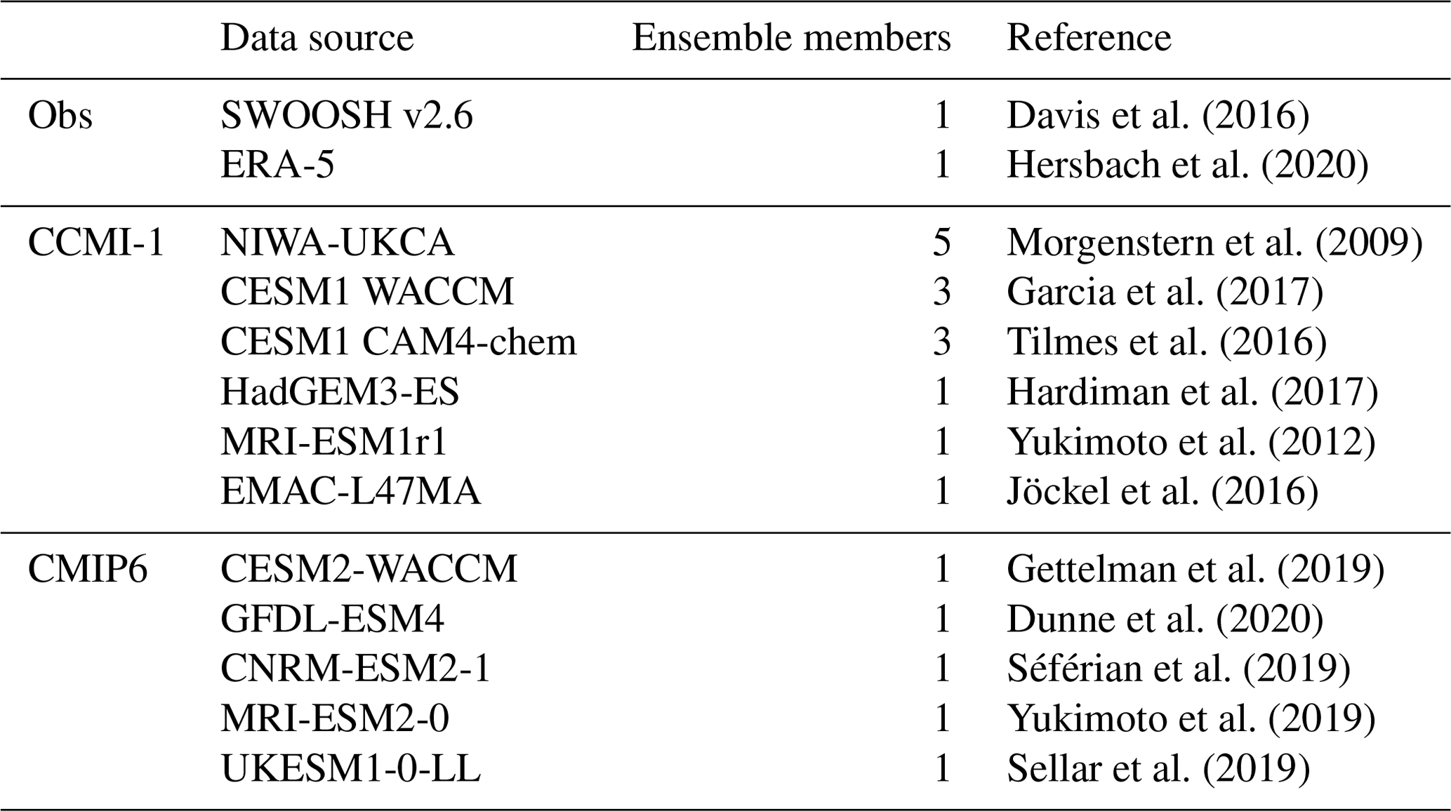
We examine six models participating in the CCMI and five coupled chemistry–climate models participating in the sixth phase of the Coupled Model Intercomparison Project (CMIP6; Eyring et al., 2016). We only include CMIP6 models with interactive stratospheric chemistry as such a coupled chemistry–climate configuration has been shown to lead to more robust interannual variability of temperatures in the lower stratosphere as compared to models with fixed ozone (Yook et al., 2020). Note that most of the models nevertheless simulate too warm a cold point and too little interannual variability of entry water (Garfinkel et al., 2021).

CCMI phase 1 was jointly launched by the International Global Atmospheric Chemistry (IGAC) and the Stratosphere-troposphere Processes And their Role in Climate (SPARC) to better understand chemistry–climate interactions in the recent past and future climate (Eyring et al., 2013; Morgenstern et al., 2017). We analyze the Ref-C2 simulations, which span the period 1960–2100, impose ozone-depleting substances as specified by the World Meteorological Organization (2011), and impose greenhouse gases other than ozone-depleting substances as in Representative Concentration Pathway (RCP) 6.0 (Meinshausen et al., 2011). More details about these simulations are included in Eyring et al. (2013). We only consider CCMI models with a coupled ocean (though for some models, e.g., EMAC, the ocean state is taken from a different integration), and we compute statistics for all available ensemble members separately before computing the average response for each model. The CCMI-1 models used in this study are listed in Table 2. CCMI-2 models are instructed to nudge the QBO rather than spontaneously simulate it. While this nudging should lead to an improved ability to capture the temperature response to the QBO (as discussed in Sect. 4), this improvement is not because the models themselves are necessarily better, and nudging is known to interfere with the transport of trace gases (Orbe et al., 2017, 2018). Hence the water vapor variability in CCMI-2 models is outside the scope of this study. Note, however, that three of the CCMI-1 models considered here nudged the QBO: the NCAR models and EMAC. The fidelity of the QBO in these models will be discussed in Sect. 4.

In addition to the CCMI-1 models, we also consider five Earth system models with coupled chemistry that are participating in CMIP6: CESM2-WACCM (Gettelman et al., 2019), GFDL-ESM4 (Dunne et al., 2020), CNRM-ESM2-1 (Séférian et al., 2019), MRI-ESM2-0 (Yukimoto et al., 2019) and UKESM1-0-LL (Sellar et al., 2019). The climatology and seasonal cycle of stratospheric water vapor in these models are documented in Keeble et al. (2021). All six models spontaneously represent the QBO (Rao et al., 2020a; Richter et al., 2020; Rao et al., 2020b), though as discussed in Sect. 4 the quality of the simulation varies. For all CMIP6 models we focus on the historical integrations of the period 1850 to 2014. Note that standard CMIP6 output includes the 70 and 100 hPa levels but unfortunately no level in between, and so our ability to diagnose physical processes near the cold point is limited (in contrast, CCMI output is available both near 80 and 90 hPa). All data are deseasonalized by subtracting the long-term monthly means for that specific data product.

Davis et al. (2016)Hersbach et al. (2020)Morgenstern et al. (2009)Garcia et al. (2017)Tilmes et al. (2016)Hardiman et al. (2017)Yukimoto et al. (2012)Jöckel et al. (2016)Gettelman et al. (2019)Dunne et al. (2020)Séférian et al. (2019)Yukimoto et al. (2019)Sellar et al. (2019)

Table 2 The data sources used in this study. For CMIP6 models we focus on the historical integrations of the period 1850 to 2014 and for CCMI phase 1 the Ref-C2 simulations spanning the years 1960 to 2100. The CCMI-1 models CESM1 WACCM, CESM1 CAM4-chem and EMAC-L47MA nudge the QBO; the rest spontaneously generate the QBO.

2.2 Target variables and indices

The target variable for all data sources is entry water, defined as water vapor at 82 hPa for SWOOSH, the closest archived level to 82 hPa for CCMI (for nearly all models this is 80 hPa), and 70 hPa for CMIP6. The Quasi-Biennial Oscillation index is derived from the 50 mb zonal wind data in the NCEP/NCAR Reanalysis Climate Data Assimilation System (Climate Prediction Center, 2012). While including levels lower than 50 hPa may lead to a slight improvement of the fit in observational data, many of the CCMI/CMIP6 models struggle to capture any remnant of the QBO below 50 hPa (Rao et al., 2020a; Richter et al., 2020; Rao et al., 2020b), and hence we use 50 hPa only throughout this paper. The lagged correlation of the QBO with near 82 hPa entry water area averaged between 15^∘ S and 15^∘ N is shown in Fig. 1a, and it is clear that a lag of 2 to 5 months maximizes the relationship in observations and in models. In Sect. 3 we use a lag of 5 months, and in Sect. 4 we use a lag of 2 months for CCMI and 5 months for CMIP6, though results are similar if the lag is changed by a few months. A later lag for the QBO is used for CMIP6 due to the difference in available pressure levels used to define entry water.

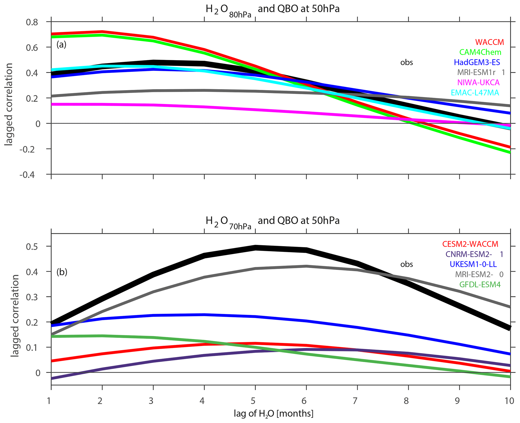
Figure 1 Lagged correlation between the QBO at 50 hPa and tropical water vapor at (a) 80 hPa in CCMI models and (b) 70 hPa in CMIP6 models (entry water is lagged after the QBO). The lagged correlation for observations (SWOOSH data) is also included as a thick black line. The combinedanomfillanomh2oq product of swoosh-v02.6-198401-201912-latpress-2.5deg-L31 is used for observations from 1994 to 2019. Note that the WACCM, CAM4Chem and EMAC-L47MA models in panel (a) nudge the QBO; in all other models, the QBO is spontaneously generated.

The El Niño–Southern Oscillation is tracked using the Niño 3.4 index (5^∘ N–5^∘ S, 170–120^∘ W), sourced with ERSSTv5 data with a 1981–2010 base period. The data are taken from NOAA (Climate Prediction Center, 2012).

The CCMI and CMIP6 integrations include both long-term changes due to climate change and interannual variability. In order to maintain focus on the latter, the analyses in Sect. 4 include, in addition to the QBO regressor, a regressor to track greenhouse gas concentrations (the equivalent CO₂ from the RCP6.0 scenario and historical CO₂ concentrations for historical simulations; Meinshausen et al., 2011). For the observational analysis, we do not include a CO₂ regressor but instead detrend all time series, for two reasons: first, the regression coefficient for CO₂ in an MLR is extremely sensitive to whether we include the HALOE period or not, and, second, the ML methods are more stable when provided with fewer predictors on which to train the model. Both of these effects likely arise because of the short duration of the observational data record.

The T500 index is the air temperature at 500 hPa averaged over the tropics (20^∘ S to 20^∘ N) taken from the ERA5.1 reanalysis (Hersbach et al., 2018; Hersbach et al., 2020). The BDC (Brewer–Dobson circulation) index is the ERA5.1 variable “mean temperature tendency due to parametrizations” at 70 hPa averaged over the tropics (20^∘ S to 20^∘ N). In the tropical stratosphere, the dominant contribution to the mean temperature tendency due to parametrizations is radiative heating.

The cold-point temperature (CPT) index is calculated as in Randel and Park (2019), who use air temperature data from three equatorial radiosonde stations, Nairobi (1^∘ S, 37^∘ E), Manaus (3^∘ S, 60^∘ W) and Majuro (7^∘ N, 171^∘ E), sourced from the Integrated Global Radiosonde Archive (IGRA) (Durre et al., 2006). The radiosonde data were resampled to monthly means, and their seasonal cycle was removed.

Note that the correlation of the BDC with the QBO is −0.66 (Fig. 2), and hence including both in a single regression or ML model can lead to erroneous model interpretation. If the BDC is defined at 82 hPa (instead of at 70 hPa), the correlation with the QBO drops, but then the correlation of the BDC with cold-point temperatures reaches −0.72 over the period since 2005. Hence there is again the potential for misleading results if both are included, and if only the BDC is included, there is ambiguity as to whether a signal is due to the BDC or rather actually is associated with CPT but appears in the BDC regression coefficient because of the tight relationship between the CPT and BDC. Finally, the correlation between T500 and ENSO is 0.52, and if we high-pass-filter the data to focus on interannual timescales, the correlation increases further. Hence there is a similar risk of misleading results if both are included in a MLR and similar ambiguity if only one is included.

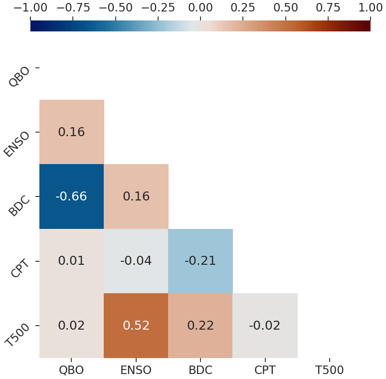
Figure 2 A correlation heat map for the predictors used in the analysis. The time span is from 1994 to 2019.

All indices are deseasonalized by removing the long-term monthly means. We do not consider seasonality in this work in order to maximize the degrees of freedom, though we certainly acknowledge that the regression coefficients for, say, ENSO change sign between midwinter and late spring (Garfinkel et al., 2018, 2021). For all of these predictor time series, we divide by the standard deviation before constructing a MLR or ML model.

As discussed in Randel and Park (2019), cold-point temperatures are highly correlated with entry water vapor (correlation of ∼0.8 from 1993–2017 for 60^∘ S–60^∘ N averaged entry water vapor). This result is reproduced here over the period 2005–2019, but showing the latitude vs. longitude distribution, in Fig. 3a. We allow the CPT to lead entry water vapor by up to 5 months. Correlations peak above 0.8, and, more generally, 75 % (i.e., the maximum R² on Fig. 3a) of the cold-point temperature and entry water variability are linearly related. We treat this 0.8 correlation as an upper bound on the effect that large-scale, monthly mean dynamics can have on entry water vapor (with the remaining 25 % due to processes on smaller spatial scales or shorter timescales). The aim of this paper is to understand the 75 % of the variability that is due to large-scale processes. In particular, to what extent can this 75 % of the variability in turn be explained by large-scale processes remote to the cold point such as the QBO and ENSO?

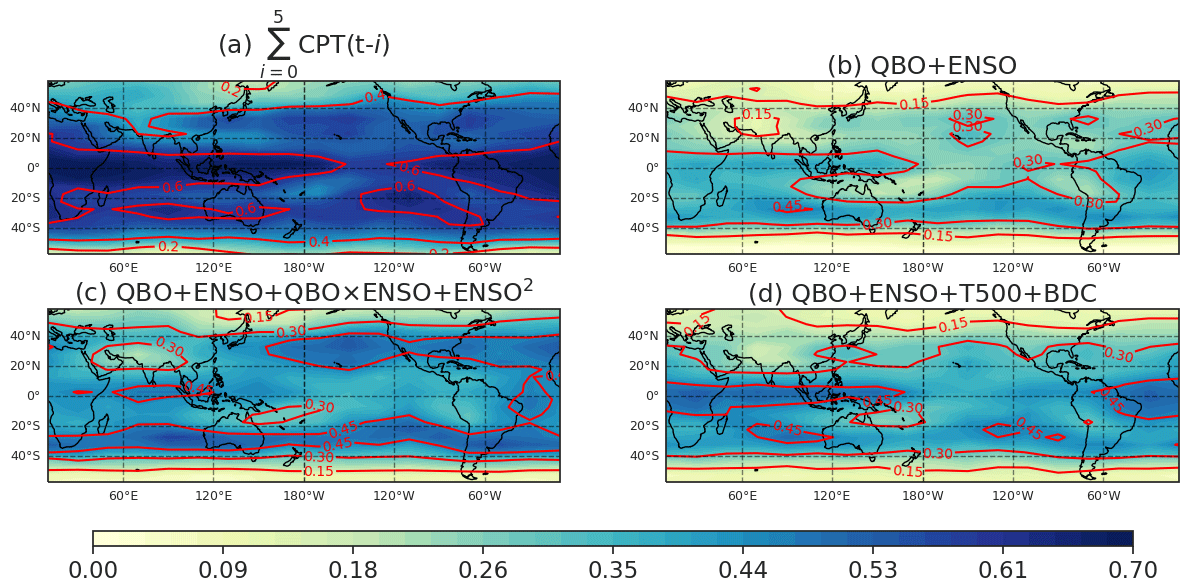
Figure 3 The R² of the MLR between water vapor anomalies at the 82.54 hPa level with the four groups of predictors: (a) cold-point temperatures, (b) QBO and ENSO, (c) as in (b) but adding in ENSO² and QBO × ENSO, and (d) as in (b) but adding in T500 hPa and the BDC. This MLR spans from 2005 to 2019 and uses the 3D SWOOSH product. The regression is reconstructed directly from all predictors, i.e., in-sample.

2.3 Machine learning (ML) models

As discussed in the Introduction, the connection between the QBO, ENSO, and entry water is not necessarily linear. Accordingly, we pick three popular types of ML models which we use in a supervised learning regression: support vector machines (SVMs), random forest (RF) and multilayer perceptron (MLP), and these ML models are applied in Sect. 3 only. All the models here are implemented through the Scikit-learn Python package (Pedregosa et al., 2011). All use an optimization scheme in order to reduce the error between the predicted and the observed target variable. However, each of the models' approach to the regression task is different.

The SVM model, in a classification task, uses a linear hyperplane in order to separate each sample class (Boser et al., 1992). By applying the kernel trick, the input variables are nonlinearly transformed into a high dimensional space where the type of the kernel, e.g., radial basis function, can be determined by hyperparameter tuning (Vapnik et al., 1995). In regression tasks, now named SVR (support vector regression), more flexibility is allowed where an error parameter is added (ϵ), which measures the constraint on the residuals. Let us consider the objective function in OLS (ordinary least-squares) which is used in MLRs:

$$\begin{array}{}\text{(1)}& \mathrm{MIN}\sum _{i=\mathrm{1}}^n(y_i-w_i\cdot x_i{)}^{\mathrm{2}},\end{array}$$

where y_i is the target, w_i is the coefficient and x_i is the predictor. The objective function in the SVR is used to minimize the coefficients (specifically the l2 norm) and not the squared error as in the OLS. The constraints handle the error term (ϵ) where it can be tuned to gain the desired accuracy of our model. Thus, SVR's objective function and constraints are as follows:

$$\begin{array}{}\text{(2)}& {\displaystyle }\mathrm{MIN}{\displaystyle \frac{\mathrm{1}}{\mathrm{2}}}|\mid w\mid {|}^{\mathrm{2}}\text{(3)}& {\displaystyle }|y_i-w_i\cdot x_i|\le \mathit{ϵ}.\end{array}$$

Other improvements to the SVR's objective function are added as additional hyperparameters, e.g., to deal with points that reside beyond the margin defined by ϵ.

The RF model operates very differently than SVM as it is based on an ensemble of decision trees which in our case solve a regression task. A regression tree algorithm is a way of splitting the data set by selecting certain points that minimize the mean squared error (MSE), defined as follows:

$$\begin{array}{}\text{(4)}& \mathrm{MSE}={\displaystyle \frac{\mathrm{1}}{n}}\sum _{i=\mathrm{1}}^n(y_i-\widehat{y}{)}^{\mathrm{2}},\end{array}$$

where y is the observation, and $\widehat{y}$ is the prediction. These points are selected through an iterative process of calculating the MSE for all the splits and choosing the split that minimizes the MSE. Regression trees are prone to overfitting, and while there are hyperparameters which can help with that, much better algorithms were developed on top of regression trees which address this issue adequately. One of these algorithms is the RF model (Breiman, 2001), which is outlined as follows:

1. Pick k data points at random from the training set.

2. Build a regression tree associated with these k data points.

3. Choose N trees to build and repeat steps 1 and 2.

4. For a new data point, iterate over the N built trees, evaluate their prediction for the data point and assign their mean prediction to this point.

Here, overfitting is also an issue though a smaller one than individual regression trees and can be dealt with by adjusting the model complexity via the various hyperparameters. The RF model uses many independent decision trees on randomized selections of the trained data subsets. The final output is produced by averaging all of the individual decision tree outputs.

The MLP is an artificial neural network that includes multilayered nodes with weights (Hinton, 1989). Typically, the network architecture includes an input layer, any number of hidden layers and an output layer, where each layer's nodes are connected via activation functions (a so-called feed-forward propagation). During the learning process, the weights are re-evaluated using the back-propagation iterative algorithm (Orr and Müller, 2003) in order to decrease the cost function. Typically, the number of hidden layers in the MLP architecture is determined in the hyperparameter tuning step and in our case was one hidden layer with 10 hidden units.

Finally, we use multiple linear regression (MLR), a well-known and often used technique in the field (e.g., Dessler et al., 2013; Diallo et al., 2018). When applied to latitude–longitude entry water vapor data, the model yields

$$\begin{array}{}\text{(5)}& {\mathit{\chi }}_{{\mathrm{H}}_{\mathrm{2}}\mathrm{O}}(t,\mathit{\varphi },\mathit{\lambda })=\mathit{\alpha }(\mathit{\varphi },\mathit{\lambda })+{\mathit{\beta }}_{\mathrm{i}}(\mathit{\varphi },\mathit{\lambda })\cdot {\mathit{\eta }}_i\left(t\right)+\mathit{ϵ}(t,\mathit{\varphi },\mathit{\lambda }),\end{array}$$

where ${\mathit{\chi }}_{{\mathrm{H}}_{\mathrm{2}}\mathrm{O}}$ is the reconstructed water vapor anomaly field, and t, ϕ and λ are the time, latitude and longitude respectively. α and β_i are the intercept and the beta coefficients of the MLR solution, ϵ is the residual field and η denotes the predictors used in the analysis. Note that this MLR has been computed separately for each grid cell using the 3D SWOOSH data since 2005. We have also performed an MLR using the tropical mean entry water since 1994, where we average the latitude range between 15^∘ S and 15^∘ N, and the predictors are QBO and ENSO. Thus, a much simpler linear model is formulated as follows:

$$\begin{array}{}\text{(6)}& {\mathit{\chi }}_{{\mathrm{H}}_{\mathrm{2}}\mathrm{O}}\left(t\right)=\mathit{\alpha }+{\mathit{\beta }}_{\mathrm{i}}\cdot {\mathit{\eta }}_i\left(t\right)+\mathit{ϵ}\left(t\right).\end{array}$$

The validation and testing procedures of the ML models are done in two stages using a 5-fold cross-validation (CV) technique for each model separately. First, for the validation stage, we randomly select 80 % of the samples and split them into five random groups called folds. Second, we train each model on four folds and test its performance (R²) on the remaining fold. Third, we repeat this process five times (hence 5-fold CV) while iterating over all the folds. These three steps are repeated for all possible combinations of the hyperparameters, and we then choose best hyperparameters which maximize the out-of-sample R². (This step is skipped for MLR since it does not have hyperparameters.) Then, for evaluating the models' performance, we traditionally would test the models once on the remaining data (i.e., the test set); however, since our data set is quite short (312 samples at most), we would like to gain understanding of the models' performance distributions. Thus, we use a similar 5-fold CV on all the samples: we randomly divide the data by 5, train each model on four folds and test its performance (R²) on the remaining fold; these steps are cycled through all five folds. This random division of the data into five folds and subsequent cycling is performed 20 times, and so we end up with 100 R² scores per each model.

In the spirit of reproducible science, we encourage the interested reader to explore the Python repository hosted on GitHub (https://github.com/ZiskinZiv/Stratospheric_water_vapor_ML, last access: 25 May 2022) that includes the processed data (except SWOOSH data sets) and procedures of this paper's analysis.

3 Re-evaluation of the importance of ENSO and the QBO in the observational record

We begin with the reconstructed entry water vapor time series in Fig. 4 as computed by four different techniques, with the QBO and ENSO used as predictors. As discussed in Sect. 2.3, we use out-of-sample testing to reduce as much as possible overfitting. Specifically, Fig. 4 shows the mean of the predicted out-of-sample water vapor from the 5-fold cross validation scheme (see Sect. 2).

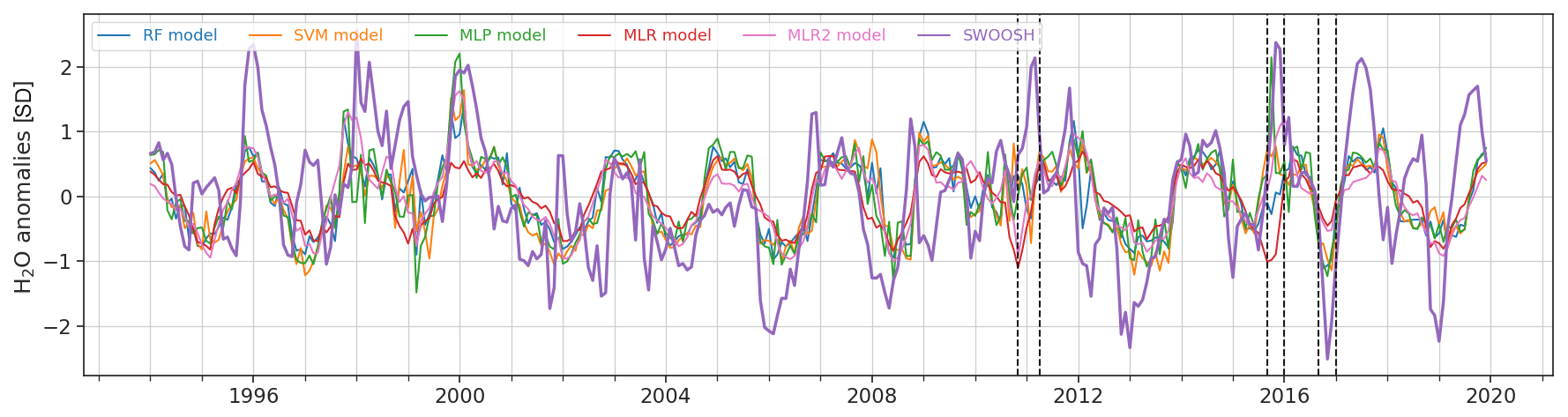
Figure 4 Out-of-sample model predictions of deseasonalized and standardized water vapor anomalies at 82.54 hPa, averaged between 15^∘ S and 15^∘ N. The various models are RF (blue), SVM (orange), MLP (green), MLR (red) and MLR2 (pink). The MLR2 model is the same as the MLR model but with ENSO² and ENSO × QBO predictors. The observations are from SWOOSH (bold purple). Note the three forecast busts: 2010-D-2011-JFM, 2015-OND and 2016-OND.

All four methods capture much of the variability of entry water present, but there are noticeably more forecast busts than if cold-point temperatures are used (see Randel and Park, 2019). Three examples of forecast busts are evident in late 2010, late 2015 and late 2016 (indicated by vertical lines), when all four techniques struggle to account for the observed change¹.

The ability of each of the four techniques is quantified in Fig. 5a–d, which shows a histogram of the R² between the predicted and actual entry water vapor for each of the individual out-of-sample tests performed. Figure 5 also indicates the mean, median and standard deviation of the histogram of out-of-sample tests and also the R² if we compute the fit using all data instead of applying an out-of-sample test. For all four techniques, there is a wide range of R² values among the 100 different out-of-sample tests, and the in-sample R² always exceeds the median of the 100 out-of-sample tests. This highlights the need to perform an out-of-sample test to minimize overfitting. If the three ML techniques are compared to MLR, the MLR is the least successful, both when applied in-sample and out-of-sample, and the three advanced ML techniques all are similarly skillful (with MLP slightly worse than SVM or RF).

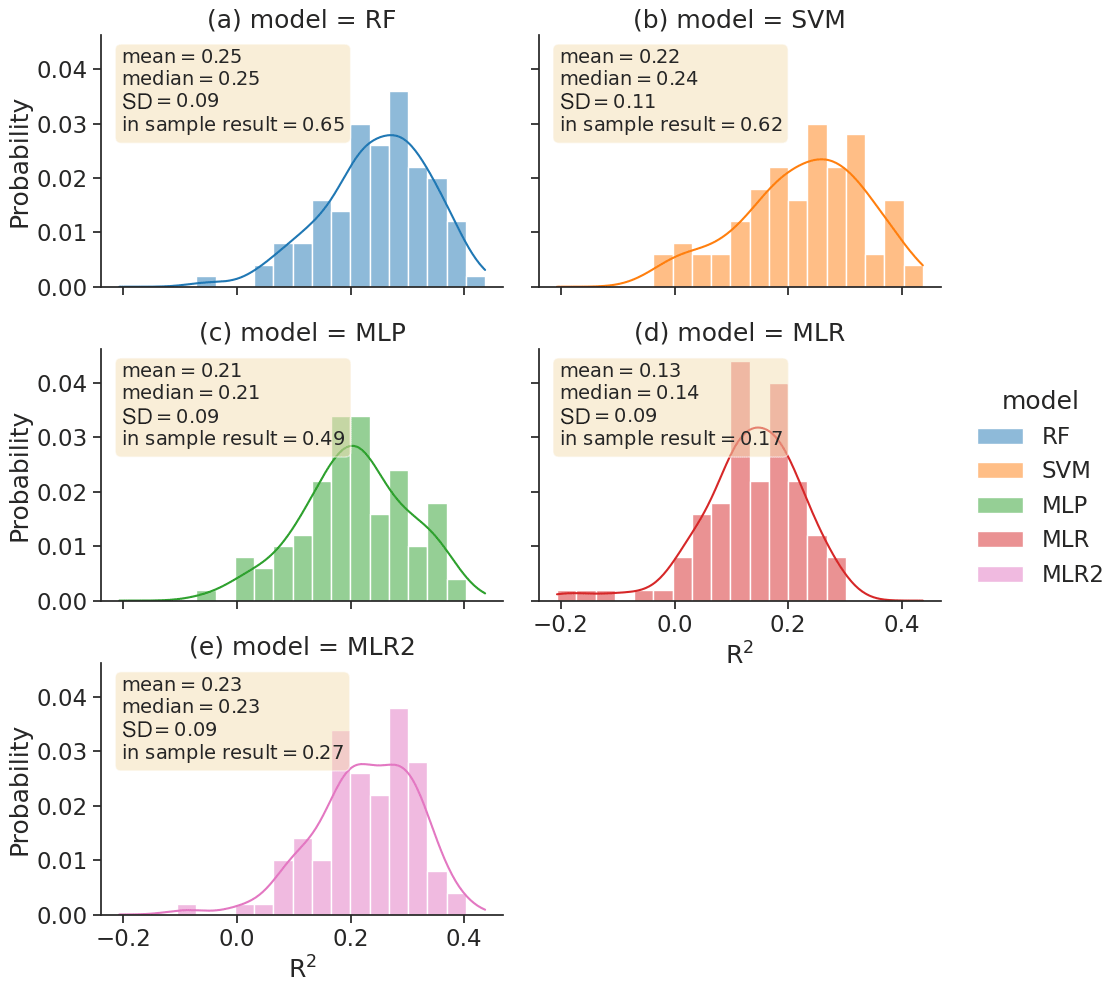
Figure 5 Out-of-sample model performance and distribution of R² scores of deseasonalized and standardized water vapor at 82 hPa, averaged between 15^∘ S and 15^∘ N. The various models are RF (blue), SVM (orange), MLP (green), MLR (red) and MLR2 (pink). The MLR2 model is the same as the MLR model but with ENSO² and ENSO × QBO predictors. The mean, median and standard deviation (SD) are noted for each distribution in a yellow text box, along with the in-sample R² score.

This comparison of MLR in Fig. 5d to the ML techniques in Fig. 5a–c may lead to an underestimate of the abilities of MLR to account for entry water vapor, as the ML techniques allow for nonlinearity but MLR does not. As discussed in the Introduction, there are at least two nonlinear processes that have been argued to exist when accounting for entry water vapor variability due to ENSO and the QBO: ENSO² and a ENSO × QBO predictor. We therefore add these two predictors to the MLR and repeat the calculation in Fig. 5e. While the in-sample result is still lower than that of the ML techniques (likely because of additional nonlinear effects that are not included in the MLR), the out-of-sample results are now similar to those of the ML techniques. Further, the busts in Fig. 4 are not any worse in MLR2 than in the ML techniques. In other words, adding these two nonlinear processes can explain most of the additional advantage of the ML techniques when the data are tested out of sample to mitigate overfitting.

Even though these nonlinear processes help, the resulting R² is still much less than that explained by CPT (Fig. 3a). Specifically, Fig. 3b shows that a MLR with just QBO and ENSO can lead to an R² ranging around 0.3; however this is only half of the R² when the actual cold-point temperatures are included (Fig. 3a). Adding the two nonlinear predictors (Fig. 3c) leads to an increase of R² by around 0.1 as compared to Fig. 3b, but this is still much less than the R² in Fig. 3a.

At least two of the techniques considered allow for a clear diagnosis of the relative importance of ENSO vs the QBO: MLR and SHapley Additive exPlanations (SHAP), as employed in the RF model. The relative importance of each of the predictors in the MLR of Fig. 5e is shown in Fig. 6, which shows a latitude vs longitude map of the regression coefficients when the regression is performed for water vapor at each grid point separately (the MLR of Fig. 5e is performed on the tropical mean water vapor.) The QBO is clearly more important than any of the other processes for accounting for entry water and thus accounts for the biennial nature of the fit in Fig. 4 with a peak-to-peak amplitude of around 0.4 ppmv. Interestingly, the map for ENSO indicates a zonally asymmetric structure (Fig. 6b), and as discussed in Yulaeva and Wallace (1994) and Garfinkel et al. (2013), the temperature response to ENSO is characterized by zonal structure, even in the lower stratosphere, with relatively warm temperatures in the Indian Ocean sector and colder temperatures in the Pacific sector. This zonal temperature dipole is thus apparently leading to a similar dipole in entry water, with moistening occurring in warm regions and drying in cold regions. The ENSO² predictor is more important than ENSO for zonal mean entry water vapor (Fig. 6b, d). The ENSO × QBO predictor is comparatively unimportant (Fig. 6c).

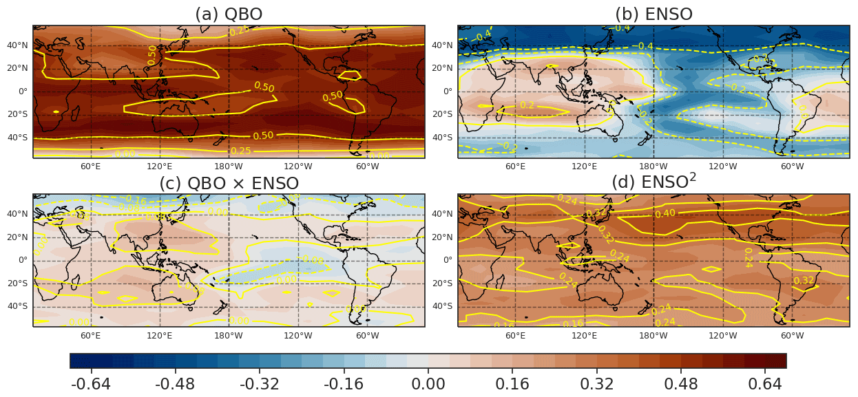
Figure 6 The in-sample β coefficients for the MLR analysis of water vapor at the 82.54 hPa level from 2005 to 2019, performed using the 3D SWOOSH data.

The SHAP technique also allows for quantification of the relative impact of ENSO versus QBO. SHAP (Lundberg et al., 2020) implements a concept borrowed from game theory, where a prediction can be explained by assuming that each predictor's value is a “player” in a game where the prediction is the payout. The Shapley values (as computed by, e.g., SHAP) indicate how to fairly distribute the “payout” among the predictors (Lundberg and Lee, 2017). The payout in our problem is the standardized entry water; thus the computed Shapley values are measuring the mean effect ENSO or QBO have on standardized H₂O anomalies. For an in-depth explanation of the SHAP technique, we encourage the interested reader to explore the SHAP chapter of the online book on explainable AI methods (Molnar, 2019).

We calculated the mean SHAP values for the predictors as trained by the RF model. QBO has a mean effect of 0.42 SD on H₂O anomalies, while ENSO has a mean effect of −0.23 SD on H₂O anomalies since it is negatively correlated with H₂O. Only when considering spring entry water is ENSO positively correlated (Garfinkel et al., 2018), though even in spring the QBO dominates. In absolute values, QBO is almost twice as important as ENSO for entry water as diagnosed by SHAP. The relative primacy of the QBO is consistent with Diallo et al. (2018) and Tian et al. (2019).

Additional evidence as to the importance of the ENSO² predictor is provided in Fig. 7, where we form an MLR using QBO and ENSO but compute the ENSO regression coefficient separately for each ENSO phase. The important point is that the regression coefficient changes sign between EN and LN (Fig. 7b vs. Fig. 7c); in other words, a more positive ENSO state during EN leads to more water vapor but so does a more negative ENSO state during LN. A naive MLR misses this effect and would imply a limited impact of ENSO on entry water vapor. Only upon considering nonlinear effects is the full impact of ENSO revealed.

Finally, some previous work has focused on using the BDC or mid-tropospheric temperatures as predictors in MLR models that attempt to explain entry water (e.g., Dessler et al., 2014). We show the R² of an MLR with these predictors in Fig. 3d. Adding T500 and the BDC clearly leads to an improved fit as compared to an MLR with only QBO and ENSO (Fig. 3b vs. Fig. 3d); however the improvement is similar to the effect of the nonlinear regressors in Fig. 3c. As discussed in Sect. 2, there is a significant correlation between the BDC at 70 hPa and the QBO at 50 hPa, and hence including both in a ML model does not lead to significant improvement. Including the BDC at 82 hPa instead leads to a larger improvement; however the BDC at 82 hPa is significantly correlated with the cold-point temperatures, and hence there is ambiguity if the BDC is defined at 82 hPa instead. There is some added value to using T500 as compared to ENSO, though as shown in Fig. 6, an ENSO predictor is much less useful than an ENSO² predictor in any event. That is, most of the improvement upon adding the nonlinear predictors comes about via the ENSO² predictor (Garfinkel et al., 2018).

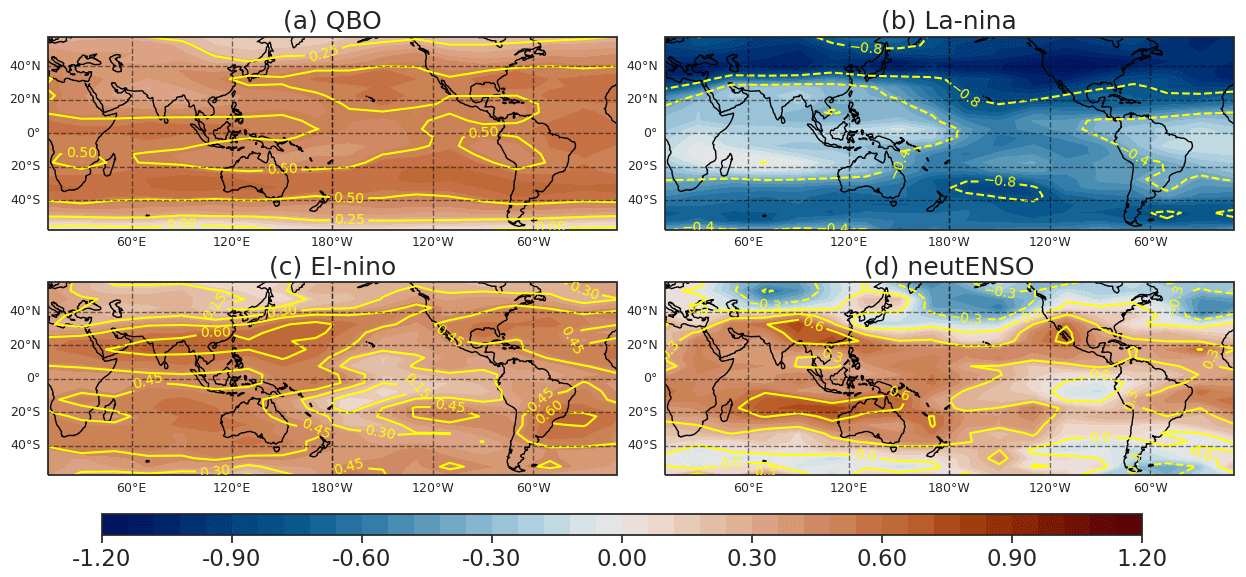
Figure 7 The in-sample β coefficients for the MLR analysis of water vapor at the 82.54 hPa level from 2005 to 2019. The ENSO predictor was separated into three parts, where EN represents the El Niño events (ENSO ≥ 0.5), LN represents the La Niña events (ENSO ≤ −0.5) and neutENSO the rest of the ENSO regressor.

4 Ability of CMIP6 and CCMI models to represent the QBO modulation

Section 3, and specifically Fig. 6, indicated that the QBO is the most important single predictor of any considered in this paper barring the cold-point temperatures themselves. We now consider the ability of CMIP6 and CCMI models to represent this connection, and for simplicity we focus on a simple regression of the QBO with entry water. (The ability of these models to represent the connection between ENSO and entry water vapor was considered in Garfinkel et al., 2021, in detail.)

The lagged correlation of the QBO with entry water is shown in Fig. 1a for the CCMI models and in Fig. 1b for the CMIP6 models. While all models capture the sign of the dependence of entry water on the QBO (an apparent improvement from Smalley et al., 2017), there is a wide range in the amplitude of the correlation. The two NCAR models in CCMI simulate the strongest relationship, but these models nudge their QBO, and the corresponding CMIP6 run with a spontaneous QBO simulates a weaker connection. Other models simulate a connection similar to (HadGEM3, EMAC-L47MA) or weaker than (NIWA-UKCA, MRI-ESM) that observed. Note that Smalley et al. (2017) considered these latter two CCMI models and also found a nearly nonexistent connection between entry water and the QBO.

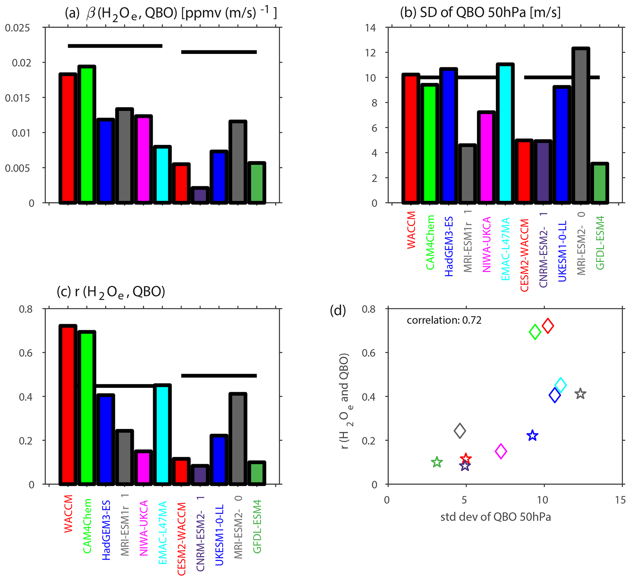
Figure 8 Relationship between the QBO and entry water vapor in CCMI and CMIP6 models. (a) Regression coefficient, (b) standard deviation of the QBO at 50 hPa, (c) correlation coefficient and (d) relationship between the correlation coefficient (panel c) and standard deviation (panel b), with the color of markers corresponding to the color used in panel (b) and (c). For (d), diamonds are CCMI models, and stars are CMIP6 models. A solid black line in panels (a)–(c) is for reanalysis. Note that entry water is defined near 80 hPa for CCMI models and at 70 hPa for CMIP6 models; hence the solid black reanalysis line differs for each. Note that the WACCM, CAM4Chem and EMAC-L47MA models included in CCMI (the first, second and sixth models in panels a, b and c; green, red and cyan) nudge the QBO; in all other models the QBO is spontaneously generated.

An alternate perspective on the ability of models to capture the relationship between the QBO and entry water is the regression coefficient from a MLR. Figure 8a shows these regression coefficients, and the observed regression coefficient is shown with a horizontal black line. The two NCAR models in CCMI (both of whom nudge the QBO) are the only models with a regression coefficient approaching that observed. The models which do not nudge uniformly underestimate the regression coefficients, and hence the relatively more realistic correlation coefficients from Fig. 1 (which are repeated in Fig. 8c) are due to biases either in the standard deviation of entry water vapor or in the standard deviation of the QBO itself. Garfinkel et al. (2021) already demonstrated that 10 of these models (with NIWA the lone exception) underestimate entry water variability. For example, EMAC-L47MA, which nudges the QBO, simulates a reasonable correlation of entry water with the QBO but a severely deficient regression coefficient due to poor interannual variability of entry water.

The models which do not nudge the QBO also mostly underestimate variability of the QBO, as shown in Fig. 8b. While, e.g., the UK Met Office model does a good job at capturing the QBO (and recall the NCAR and EMAC-L47MA CCMI models have a nudged QBO), most other models struggle. A notable improvement is evident from the MRI contribution to CCMI to the MRI contribution to CMIP6. The net effect of too weak an internal variability of the QBO or of entry water is that the regression coefficient of a model will be lower than that in observations, even if the correlation is generally realistic.

Do models with a better QBO perform better at capturing the relationship between entry water and the QBO? Figure 8d compares for each model the standard deviation of the QBO (x axis) with the correlation between entry water and the QBO (y axis), and it is evident that the two are linked. The correlation coefficient across all models is statistically significant at the 95 % level. Hence, an improved QBO leads to an improved representation of interannual variability of entry water.

5 Discussion

Stratospheric water vapor plays a crucial role in the climate system, both as a greenhouse gas that modulates the Earth's radiative budget and as a trace gas that regulates the severity of ozone depletion (Solomon et al., 1986; Forster and Shine, 1999; Solomon et al., 2010; Dessler et al., 2013; Wang et al., 2017; Banerjee et al., 2019). This study aims to understand the importance of nonlinearity for two processes – ENSO and the QBO – that have been shown to regulate water vapor concentrations on interannual timescales and to consider whether comprehensive models used for climate change assessments represent these factors correctly.

Both the QBO and ENSO are important for entry water vapor; however a simple linear perspective would lead to the mistaken conclusion that the effect of ENSO on zonal mean entry water vapor is minimal (Fig. 6b). Rather, ENSO² is the more important contributor (Fig. 6d), though even ENSO² is less important than the QBO (Fig. 6a). A multiple linear regression model that includes ENSO and the QBO performs notably worse than machine learning techniques that do not assume linearity (Fig. 5a–d); however adding an ENSO² predictor to a multiple linear regression model fills the gap in performance (Fig. 5e), and the added value from the more complicated machine learning techniques is small. The physical motivation for such an ENSO² predictor was already presented in Garfinkel et al. (2018).

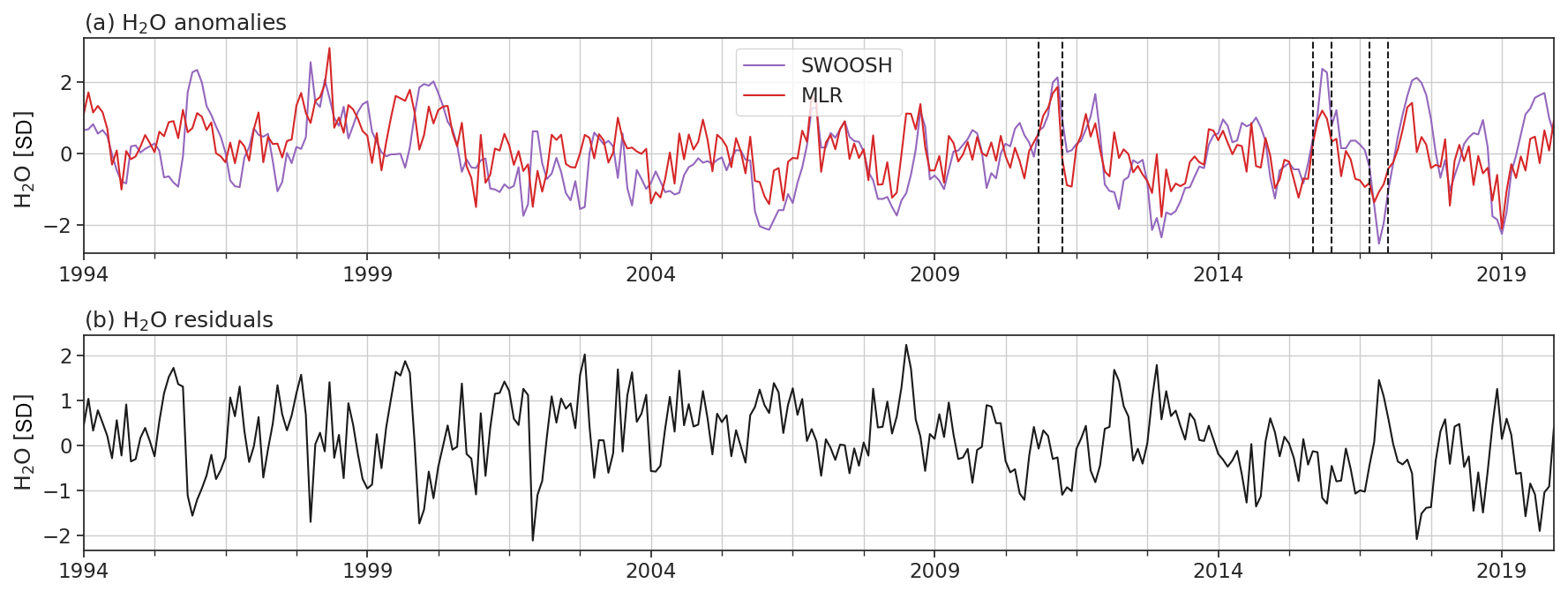
Figure 9 (a) Deseasonalized and standardized water vapor at 82.54 hPa averaged between 15^∘ S and 15^∘ N (purple) and their MLR reconstruction (red) and residuals, spanning from 1994 to 2019. This MLR analysis was carried out with the Randel and Park (2019) CPT as the only predictor but after detrending the data. The MLR model was trained on the MLS portion of SWOOSH (2005 to 2019; correlation = 0.68) and was reconstructed on the full time span (1994–2019; correlation = 0.59). (b) The residuals from the MLR reconstruction.

Most of the comprehensive models considered here underestimate the strength of the connection between the QBO and entry water vapor (Figs. 1 and 8), with the only exception models which nudge the QBO rather than spontaneously generate it. While this result is disappointing, a notable improvement is evident from the CCMVal2 and the early CCMI data analyzed by Smalley et al. (2017). We find that models in which the QBO reaches the lower stratosphere tend to perform better at capturing the relationship between entry water and the QBO (consistent with Geller et al., 2016), and QBO propagation into the lowermost stratosphere is also crucial for QBO teleconnections to the subtropical jet, to the Arctic stratosphere and to tropical convection (Garfinkel and Hartmann, 2011; Garfinkel et al., 2012; Martin et al., 2021).

When considering the total variance of entry water vapor in Fig. 5, the out-of-sample R² was always less than the in-sample R². The importance of out-of-sample testing is further illustrated in Fig. 9. Figure 9a shows the time series of zonal mean water vapor from SWOOSH and the MLR reconstruction if the detrended Randel and Park (2019) CPT is used as the sole predictor for detrended entry water and the model is trained over the period 2005 to 2019 only. While the MLR model does a reasonable job of explaining the observed variability over the period used for training the MLR model, the MLR fails when applied out-of-sample to the pre-MLS period (Fig. 9b), as reflected by the generally larger values of the residuals. In other words, the model is overfit to the training data and is not generalizing well to out-of-sample data. This kind of overfitting can be minimized by appropriately tuning the hyperparameters for the ML techniques, though for MLR the only remedy is to perform out-of-sample testing. Hence we strongly recommend that future studies using MLR or similar techniques use some variant of out-of-sample testing to minimize overfitting.

While the ENSO predictor is only weakly related to zonal mean entry water vapor, ENSO is associated with zonal structure in water vapor in the lower stratosphere. Figure 6b shows that water vapor is enhanced over the Indian Ocean sector and reduced over the eastern Pacific sector (see also Figs. 4 and 11 of Konopka et al., 2016, for a similar feature at θ=390 K). This zonal dipole resembles the zonal dipole of temperature in the tropical tropopause layer (TTL; e.g., Garfinkel et al., 2013, 2018), with locally warm TTL conditions associated with moistening and locally cold TTL conditions associated with drying. Note that higher in the stratosphere, this zonal dipole goes away. However this result suggests that up to 82 hPa horizontal motion is still not fast enough to fully homogenize tropical water vapor, as might be expected if the tape recorder mechanism were the only relevant mechanism (Mote et al., 1996b). Future work should consider whether other factors (e.g., sea surface temperature (SST) patterns not related to ENSO) may also lead to zonal structure of water vapor in the lower stratosphere. Future work should also consider additional novel means of interpreting the improvements of the ML fits as compared to MLR, in order to bridge the gap between an improved fit and an understanding of how and why the improvement came about.

Finally, cold-point temperatures (CPTs) control around 75 % of the variance of entry water vapor over the historical record. None of the large-scale predictors, neither individually nor in combination, come even close to explaining such a large fraction of the variance (Fig. 3). This gap in explainable variance highlights the need to better understand CPT variability on interannual timescales and perhaps even to build predictive models for the CPT itself.