Technical note: Interpretation of field observations of point-source methane plume using observation-driven large-eddy simulations

This study demonstrates the ability of large-eddy simulation (LES) forced by a large-scale model to reproduce plume dispersion in an actual field campaign. Our aim is to bring together field observations taken under non-ideal conditions and LES to show that this combination can help to derive point-source strengths from sparse observations. We analyze results from a single-day case study based on data collected near an oil well during the ROMEO campaign (ROmanian Methane Emissions from Oil and gas) that took place in October 2019. We set up our LES using boundary conditions derived from the meteorological reanalysis ERA5 and released a point source in line with the configuration in the field. The weather conditions produced by the LES show close agreement with field observations, although the observed wind field showed complex features due to the absence of synoptic forcing. In order to align the plume direction with field observations, we created a second simulation experiment with manipulated wind fields that better resemble the observations. Using these LESs, the estimated source strengths agree well with the emitted artificial tracer gas plume, indicating the suitability of LES to infer source strengths from observations under complex conditions. To further harvest the added value of LES, higher-order statistical moments of the simulated plume were analyzed. Here, we found good agreement with plumes from previous LES and laboratory experiments in channel flows. We derived a length scale of plume mixing from the boundary layer height, the mean wind speed and convective velocity scale. It was demonstrated that this length scale represents the distance from the source at which the predominant plume behavior transfers from meandering dispersion to relative dispersion.

1 Introduction

The reduction of greenhouse gas (GHG) emissions is of the highest importance in mitigation of climate change. Methane (CH₄) is one of the most potent GHGs, but due to its relatively short lifetime in the atmosphere, reduction of CH₄ emissions can have more immediate positive effects on the mitigation of climate change effects (e.g., Baker et al., 2015; Zickfield et al., 2017; Caulton et al., 2018). Methane has a large variety of sources that differ in origin (anthropogenic or natural) and size (e.g., point-like, diffuse, line). An overview of different source types and their contribution to the global methane budget is given by Saunois et al. (2016).

In order to help constrain methane emissions, the Methane goes Mobile – Measurements and Modelling (MEMO²) project started in 2017. The goal of the project was to improve CH₄ emission factors in inventories on the European scale by combining extensive measurement campaigns of different sources of CH₄ with modeling techniques across different scales. The MEMO² consortium participated in a campaign in which methane emissions from the Romanian oil and gas industry (ROMEO, ROmanian Methane Emissions from Oil and gas) were sampled. The campaign took place during October 2019. Sources of methane were measured on basin and well scales employing various measurement techniques.

With methane often being released from small but strong sources in a turbulent atmosphere, the observation of plumes is challenging. A large variety of measurement techniques have been developed for identification and quantification of GHG sources, ranging from satellite based observations (e.g., Bergamaschi et al., 2007; Jacob et al., 2016) and basin-scale measurements using aircraft (Conley et al., 2017) to local source measurement techniques. These local techniques include, among others, instruments placed on unmanned aerial vehicles (UAVs) (e.g., Andersen et al., 2018; Shah et al., 2020), instruments placed on ground vehicles (e.g., Hensen et al., 2006; Baillie et al., 2019) and point measurements from sensors mounted on towers (Röckmann et al., 2016). Each of these techniques has its own strengths, either being highly accurate in time or covering large spatial areas, but neither technique does both. Dispersion models provide insight into the behavior of plumes and can help with the data interpretation and planning of measurement strategies. These models vary greatly in their complexity and underlying assumptions. Most commonly, Gaussian plume models are combined with observations to quantify sources (Caulton et al., 2018; Edie et al., 2020; Rybchuk et al., 2020). These simple models are fast and easy to use but come with restrictive assumptions (e.g., stationarity of the plume and the mean wind) that make their application challenging under the strongly transient conditions that often characterize the local atmospheric boundary. With the development of computer power in the past decades and of high-resolution models that are able to simultaneously resolve the turbulent velocity field and describe the transport of emitted tracers, large-eddy simulations (LESs) have been increasingly used for plume studies (Cassiani et al., 2020). LESs explicitly resolve the largest eddies, which carry most of the energy, and parameterize the smallest scales using subgrid-scale models (e.g., Deardorff, 1973; Pope, 2000). LESs have been utilized in many dispersion studies, mostly focusing on idealized channel flows in various stability regimes (e.g., Dosio and de Arellano, 2006; Boppana et al., 2012; Ardeshiri et al., 2020). LESs have been successfully validated (e.g., Dosio and de Arellano, 2006; Ardeshiri et al., 2020) against a considerable number of extensive laboratory dispersion studies. These dispersion studies include channel flows in either water or air (e.g., Fackrell and Robins, 1982a, b; Gailis et al., 2007; Nironi et al., 2015). One of the main advantages of LES in dispersion studies is that it provides a high temporal and spatial resolution of the 3D plume. This enables detailed analysis of the plume statistics, something which is difficult to do only from observations. Furthermore, LES can be used as a laboratory for optimizing measurement strategies. Despite the huge number of idealized studies, the performance of LES has not been validated against many experimental field studies. (Steinfeld et al., 2008; Ardeshiri et al., 2020; Rybchuk et al., 2020). For instance, the Prairie Grass experiment (Barad, 1958) still serves as a common reference for LES studies. More recently, Caulton et al. (2018) evaluated the performance of the Gaussian plume model against measurements in a neutral atmosphere and LES, while Rybchuk et al. (2020) evaluated Weather Research and Forecasting (WRF) LES with the Prairie Grass experiment for convective conditions.

In this study, we aim to bring together actual field observations under less than ideal conditions with LES. The ROMEO campaign focuses on sampling methane from spatially distributed sources covering a large area using mobile measurement techniques. While this approach is very useful in detecting unknown sources, measurements of individual, isolated plumes are often sparse. This is due to the measurement techniques employed. For example, plume transects using cars only provide observations at the surface in one dimension. Moreover, this observation strategy is limited by the conditions in the field (accessibility of the source, the number of adjacent roads on which measurements can be taken, road conditions, etc.). Here, we aim to demonstrate how LES can help in interpreting sparse observations in the field both from a viewpoint of validation and interpretation. We will present an LES dispersion study of a methane plume measured during the ROMEO campaign. The LES study is set up combining local meteorological observations with ECMWF ERA5 (Hersbach et al., 2020). We will compare the measured plume with the LES plume in order to gain insight into the information gathered through the measurement process and to evaluate the performance of LES. Finally, we will use LES to study the structure of the simulated plume in convective conditions and its behavior by analyzing the higher-order statistical moments. We will build on the idealized studies (Dosio and de Arellano, 2006; Cassiani et al., 2020) and apply the statistical analyses to simulations that represent realistic field conditions.

The structure of this paper is as follows. In Sect. 2 we introduce the location where the measurements took place and look at the meteorological conditions relevant for the plume dispersion. Following this, in Sect. 2.2 we present available data from the campaign as well as the methods and instruments employed in the field. In Sect. 3 we present the numerical model used to perform the LES, the simulation setup and forcing used to reproduce the meteorological conditions. In this section we will also outline the statistical methods used to inspect the simulated plume behavior. In Sect. 4 we evaluate the LES plume with observation and discuss the characteristics of both plumes. This is followed by a more in-depth analysis of the simulated plume at various distances from the source. Finally, in Sect. 5 we evaluate the usability of LES for dispersion studies under realistic meteorological conditions.

2 Case description

2.1 Site description and meteorological conditions

The case study presented here is based on measurements performed by a team from the Netherlands Organisation for Applied Scientific Research (TNO) during the ROMEO campaign in Romania. The measurements were taken in Parhova County at oil well 1474 in Dărmănești. The county is located in the region between the Transylvanian Alps and Bucharest, which is characterized by plains in the south and the Carpathian mountains in the north. The actual site is located in the central part of the county, where the two distinct landscapes meet. The measurements were performed on the road downwind from an oil well over the course of 3 h. The length of the road segment on which the plume was measured was 150 m, while the distance from the middle of road to the well was 78 m. The measured well and the adjacent road on which measurements were performed is shown in Fig. 1b, and the vehicle used to perform the measurements is shown in Fig. 1a.

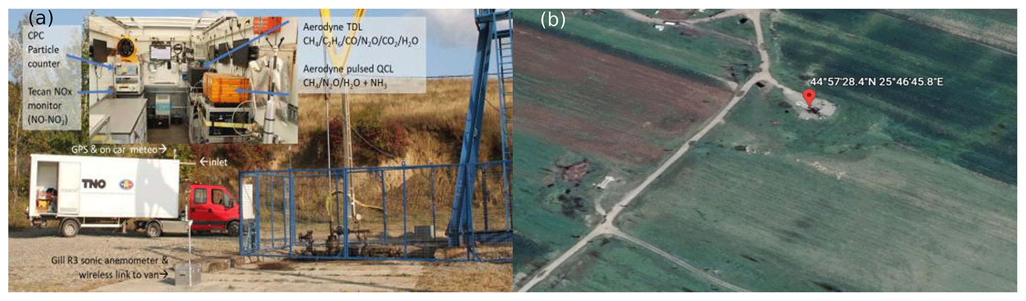
Figure 1 (a) (Inset figure) The measurement setup inside the TNO vehicle. (Main figure) The TNO vehicle used in the measurement campaign, the location of the inlet is indicated on the figure. (b) Google Earth view of the measurement site with the oil well location pointed out. © Google Earth, Maxar Technologies.

The measurements were performed in the afternoon (14:30–17:30 LT (UTC+3 h)) on 17 October 2019. The weather at the location was characterized by very low speed winds and no cloud cover, as confirmed by the participants of the campaign. To analyze the overall synoptic situation over Europe and Romania in particular, we used the geopotential height and temperature chart obtained from ERA5 (Hersbach et al., 2020). The weather over Romania was characterized by very low gradients in both temperature and pressure (Fig. 2a), resulting in low wind speeds and advection during the campaign. Hence, we expect that the conditions were strongly influenced by local convection.

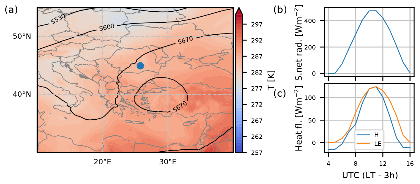
Figure 2 Meteorological situation over SE Europe on 17 October 2019. (a) Geopotential height (m) at the 500 hPa pressure level and temperature at 850 hPa at 12:00 UTC. The location of the studied region is indicated on the map by a blue circle. (b) Surface net solar radiation; (c) hourly values of sensible and latent heat at the location of the measurements.

Fig. 2 shows the surface net solar radiation and the sensible and latent heat fluxes in the region (panels b and c, respectively) retrieved from the ERA5 data. The surface heat fluxes are comparable, indicating dry conditions (Fig. 2b), and the solar radiation indicates no clouds were present. Furthermore, it was inferred from the ERA5 data that the temperature maximum at the surface was 22 ^∘C and that the boundary layer (BL) depth reached 700 m at 12:00 UTC (not shown). The ERA5 height wind profiles show wind turning with height. Maxima in wind speeds in opposite direction from those at the ground were seen at approximately 1000 m height or just above the BL top. For the duration of the measurements, the mean horizontal wind at the surface showed variation of 10^∘ (not shown).

As will be presented later in Fig. 3, we find that, for the duration of the measurements, the temperature at the 1000 hPa level remained almost constant and showed an almost linear decrease with height. Similarly, the specific humidity showed peak values at the surface and constant values in the mixing layer above it. Above the BL, specific humidity decreased with height. The near-constant-in-time height profiles of specific humidity and temperature confirm that the contribution of large-scale advection was negligible during the campaign. As a result, the time evolution of temperature and humidity was determined by local processes. This leads to a complex pattern in vertical baroclinicity, which is a challenge for both collecting experimental data and simulation studies.

2.2 Measurement instruments and available data

The measurement device used was a dual-laser trace gas monitor based on tunable infrared laser direct absorption spectroscopy (TILDAS; Aerodyne Research Inc., Billerica, USA) that measures methane and ethane (CH₄ and C₂H₆) simultaneously. The ethane data are used to discriminate methane plumes originating from fossil-fuel-related sources (which contain ethane) and agricultural or biomass degradation methane emissions. The instrument also measures H₂O, CO₂, CO and N₂O. The molar fractions of these components are measured at sub-ppb resolution with one measurement per second (1 Hz). Molar fractions were calibrated versus working standards for CH₄ (B20 flasks with compressed air at 2800 and 5000 ppb) that are linked to the Integrated Carbon Observation System (ICOS) and the National Oceanic and Atmospheric Administration (NOAA) standards used at the Cabauw tall tower in the Netherlands. B20 flasks are 20 L cylinders that hold 2000 L of gas at the pressure of 100 bar. Besides that, during the Romania campaign, calibration cylinders from Utrecht University were used, with molar fractions of 6.3, 27 and 130 ppm for the higher molar fraction measurements. The instrument measured CH₄, C₂H₆, N₂O, CO₂ and CO simultaneously at 1 Hz with a precision of 2.4, 0.1, 386.3 and 2. ppb, respectively. Here, precision is reported as 3 times the standard deviation of 6 min constant molar fraction readings. The instrument was placed into a vehicle that drove along the closest road and its position was logged at 1 Hz with a GPS system. The inlet of the measurement device was placed at the top of the vehicle at a height of 3 m. A delay-time correction is applied to the data to compensate for the 1.5 s delay between the logged GPS location and actual measurement in the TILDAS instrument.

A controlled release of tracer gas N₂O was conducted simultaneously with the CH₄ measurements. N₂O was released using a critical orifice of 0.65 mm² at 5 bar. Before and after the release, the mass of the cylinder was determined. Release was 0.59 ± 0.02 g s⁻¹

The wind speeds (u, v, w) were measured from a battery-operated Gill R3 sonic anemometer placed close to the source and at 1.8 m above ground level. The sonic data were stored at 20 Hz, and 1 Hz values were transmitted with a wireless link to the central computer in the van. For this analysis, 1 min averages of wind speeds were used.

Due to the varied road conditions, the vehicle speed varied from transect to transect. Therefore, the measured plumes have a different number of measured points, and the exact distribution of these points over the measurement transect differs. To obtain a uniform dataset, two end points were selected that encompass all plumes. Values of the vehicle location, CH₄ and N₂O data were linearly interpolated on a 250 point grid.

3 Numerical methods

Large-eddy simulations were performed using the MicroHH model, which is an open-source computational fluid dynamics code (van Heerwaarden et al., 2017). The code solves conservation equations of energy, momentum and mass under the anelastic approximation. The transport of passive scalars is solved with the advection–diffusion equation. The second-order Smagorinsky model is used for the subgrid parametrization of the velocity components.

Time integration is performed using a third-order accurate Runge–Kutta scheme, and the spatial domain is discretized on a staggered Arakawa C-grid.

The advection term for dispersing scalars in the model is solved using a second-order energy-conserving scheme. For atmospheric transport, positivity in numerical schemes plays a crucial role. By imposing positivity using a flux limiter, overshoots and undershoots are avoided in areas with strong concentration gradients (Hundsdorfer et al., 1995).

A periodic boundary condition was imposed for the momentum and thermodynamic variables on the lateral boundaries of the domain. The lower boundary had no-slip ($u=v=\mathrm{0}$) and no-penetration (w=0) boundary conditions, while the upper boundary had free-slip boundary conditions, with tangential components of velocity being zero ($\frac{\partial u}{\partial z}=\frac{\partial v}{\partial z}=\mathrm{0}$). The inflow and outflow boundary conditions for the scalar representing CH₄ were imposed at the lateral boundaries of the domain to prevent the plume from re-entering. The boundaries were set using Neumann (right and lower boundaries) and Dirichlet (left and lower boundaries) boundary conditions, which were used to interpolate values of scalars in two ghost cells outside of the domain.

In order to achieve LES that corresponds to the field conditions, large-scale forcings of relevant variables are imposed by coupling the LESs with the ERA5 data (Hersbach et al., 2020). The geostrophic wind and large-scale advection terms are interpolated from the ERA5 data, while the nudging of the simulation is applied on a relevant timescale to prevent the simulation from drifting from the large-scale mean profiles, as smaller-scale turbulence can still develop independently. The coupling is based on Schalkwijk et al. (2015).

3.1 Simulation setup

The LES was performed in a three-dimensional domain of 4.8 × 4.8 × 3.085 km (x, y and z directions, respectively). The domain was discretized on a 960 × 960 × 480 (x, y, z) grid. This results in uniform horizontal resolution of 5 m, while the vertical direction is resolved on a stretched grid with 2 m resolution in the first 1 km of the domain and 50 m at the top. The resolution was chosen with computational feasibility in mind such that the grid was dense enough for the dispersion to be well represented but still have the domain large enough to capture the meteorological effects relevant for this study.

A constant source of passive scalar was added as a two-dimensional Gaussian placed on the bottom of the domain. The Gaussian had the 1σ_i (i=x, y) value equal to the size of one grid box; therefore, 97 % of the source was spread on the 20 × 20 m² grid. It has been shown in laboratory studies of plume dispersion that the ratio of the source size and the size of larger-scale eddies has a significant impact on plume statistics (Fackrell and Robins, 1982a, b; Nironi et al., 2015). To circumvent this issue, the size of the source should be larger than the size of one grid box. Recently, Ardeshiri et al. (2020) investigated the influence of resolution on the flow and plume statistics in LES. They have shown that the scalar variances converge for the sources resolved by at least 4³ grid nodes. We have placed the source in the top right corner of the domain at the position (3600, 3600) m, where the domain origin is defined at the lower left corner. The scalar was emitted with a constant flux of 1 g s⁻¹.

In order to reproduce meteorological conditions encountered on the measurement day, the simulation was nudged according to height profiles of horizontal wind speed, temperature and specific humidity obtained from the ERA5 data. Large-scale forcing was imposed through geostrophic wind with the Coriolis parameter for this latitude being $f_{\mathrm{C}}=\mathrm{1.0305}\times {\mathrm{10}}^{-\mathrm{4}}$ s⁻¹. Furthermore, roughness lengths of z_0h=0.001 m and z_0m=0.05 m were imposed on the lower boundary for scalar and momentum, respectively.

The simulation was run for 7.5 h in total. A spin-up time was imposed to have the boundary layer fully developed and resembling field conditions as closely as possible. First, the fields from ERA5 were initiated at 07:00 UTC, and the simulation was started with an integration time step of 6 s. The simulation was run for 7.5 h with vertical profiles being nudged towards ERA5 profiles every hour. At 11:00 UTC, the source was activated in the simulation. The instantaneous plume concentrations c; wind components u, v, and w; and liquid potential temperature θ_l were recorded on various two-dimensional cross-sections of the domain.

The mean wind in this simulation shows fluctuating behavior, which influences the direction of the plume dispersion. Here, we assume that the local wind that influenced the dispersion was governed by local influences that are not captured in ERA5. To be able to still compare the plume at different simulation times, the mean wind speed between observations and simulation should be aligned. Therefore, we performed another simulation in which the mean wind was directed along the x axis, while keeping all the other specifics, apart from the source location, identical. These two simulations will be further on referred to as realistic and idealized for the first and second simulations, respectively. The overview of the specifics of the two simulations is given in Table 1. Note that in the idealized simulation the nudging profiles for potential temperature and specific humidity still originate from the ERA5 dataset. For the wind, however, we set the height profile of the v component in the nudging profiles to zero and set the u profile to a constant value of 3 m s⁻¹. This wind speed was chosen through manual tuning to get a good match with the measured wind speed at 2 m height. In this way the wind direction was kept constant without loosing the general characteristics of the realistically simulated boundary layer.

Table 1 The specifics of the two performed simulations. The first row shows the setup of the simulation with highly turning mean wind, and the second row shows the setup of the simulation with the mean along the x axis.

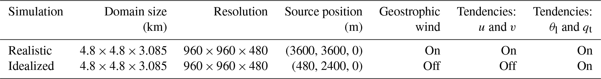
Figure 3 The nudging height profiles and the hourly-mean height profiles of variables from the simulation with centered mean horizontal wind direction.

3.2 Estimation of the unknown emission rate

Source quantification from one-dimensional transect measurements is often performed using a mass balance approach. This method compares the total line-integrated flux of the time-averaged plume from an unknown source with the flux from a known source under the same atmospheric conditions and at the same downwind distance from the source. This method has been used in conjunction with either a tracer release or – if no tracer is co-emitted – with simple plume transport models such as the Gaussian plume model (e.g., Caulton et al., 2018). The equation used for this approach reads as follows:

$$\begin{array}{}\text{(1)}& Q_{\mathrm{estim}}={\displaystyle \frac{\sum _y{C}_{\mathrm{meas}}\stackrel{\mathrm{‾}}{u_{\mathrm{meas}}}}{\sum _y{C}_{\mathrm{ref}}\stackrel{\mathrm{‾}}{u_{\mathrm{ref}}}}}\times Q_{\mathrm{ref}}.\end{array}$$

Here the Q_estim is the emission rate of the unknown source (in g s⁻¹); C (g kg⁻¹) and $\stackrel{\mathrm{‾}}{u}$ (m s⁻¹) denote the time-averaged measurements and the mean wind speed, respectively. Subscripts “ref” and “meas” refer to the reference tracer with known source Q_ref and measured tracer, respectively. Note that the reference plume can be either measured or inferred from a model.

3.3 Statistical properties of the modeled plume

Finally, we present a short overview of the statistical moments calculated for the simulated plumes that will be discussed in Sect. 4.2.1–4.2.3. Higher-order statistics can provide further insight into the behavior of the measured plume but are often unattainable from the measurements due to insufficient spatial and temporal resolution. Figure 4 shows a scheme of an idealized plume emitted from a ground point-source. Let z be the vertical position of a particle in an instantaneous plume at a distance x from the source. This plume is characterized by its centerline position z_m defined as its center of mass:

$$\begin{array}{}\text{(2)}& z_m(x,t)={\displaystyle \frac{\int c(x,y,z,t)z\mathrm{d}z\mathrm{d}y}{\int c(x,y,z,t)\mathrm{d}z\mathrm{d}y}}.\end{array}$$

An ensemble of such instantaneous plumes will have its own centerline position $\stackrel{\mathrm{‾}}{z_m}$ defined as the mean over all the realizations. Now the fluctuations of the instantaneous plume around these mean positions can be defined. The absolute fluctuation z^′ is the displacement of the particle in the plume from the mean centerline position $\stackrel{\mathrm{‾}}{z_m}$, relative fluctuation $z_r^{\prime }$ is the displacement from the instantaneous plume centerline z_m and the fluctuation of the instantaneous plume centerline $z_m^{\prime }$ is the displacement from the mean position $\stackrel{\mathrm{‾}}{z_m}$. These can be written as

$$\begin{array}{}\text{(3)}& z^{\prime }=z-\stackrel{\mathrm{‾}}{z_m},z_r^{\prime }=z-z_m,z_m^{\prime }=z_m-\stackrel{\mathrm{‾}}{z_m}.\end{array}$$

The mean plume positions and the displacements in the y direction can be defined in a similar manner.

Following the definition of Nieuwstadt (1992), the absolute plume dispersion (or the second-order moment) in the vertical direction is written as

$$\begin{array}{}\text{(4)}& {\mathit{\sigma }}_{za}^{\mathrm{2}}(x,t)={\displaystyle \frac{\int c(x,y,z,t){z^{\prime }}^{\mathrm{2}}\mathrm{d}y\mathrm{d}z}{\int c(x,y,z,t)\mathrm{d}y\mathrm{d}z}}.\end{array}$$

The absolute plume dispersion can be decomposed into its meandering and relative contributions: dispersion due to movement of the plume centerline (or meandering) and diffusion of particles from the plume centerline. Therefore, it holds that

$$\begin{array}{}\text{(5)}& {\mathit{\sigma }}_{za}^{\mathrm{2}}={\mathit{\sigma }}_{zm}^{\mathrm{2}}+{\mathit{\sigma }}_{zr}^{\mathrm{2}},\end{array}$$

where

$$\begin{array}{}\text{(6)}& \begin{array}{rl}& {\mathit{\sigma }}_{zm}^{\mathrm{2}}(x,t)={\displaystyle \frac{\int c(x,y,z,t){z_m^{\prime }}^{\mathrm{2}}\mathrm{d}y\mathrm{d}z}{\int c(x,y,z,t)\mathrm{d}y\mathrm{d}z}},\\ & {\mathit{\sigma }}_{zr}^{\mathrm{2}}(x,t)={\displaystyle \frac{\int c(x,y,z,t){z_r^{\prime }}^{\mathrm{2}}\mathrm{d}y\mathrm{d}z}{\int c(x,y,z,t)\mathrm{d}y\mathrm{d}z}}.\end{array}\end{array}$$

The third-order moment is therefore

$$\begin{array}{}\text{(7)}& \begin{array}{rl}& {\stackrel{\mathrm{‾}}{z_a}}^{\mathrm{3}}(x,t)={\displaystyle \frac{\int c(x,y,z,t){z^{\prime }}^{\mathrm{3}}\mathrm{d}y\mathrm{d}z}{\int c(x,y,z,t)\mathrm{d}y\mathrm{d}z}},\\ & {\stackrel{\mathrm{‾}}{z_r}}^{\mathrm{3}}(x,t)={\displaystyle \frac{\int c(x,y,z,t){z_r^{\prime }}^{\mathrm{3}}\mathrm{d}y\mathrm{d}z}{\int c(x,y,z,t)\mathrm{d}y\mathrm{d}z}},\\ & {\stackrel{\mathrm{‾}}{z_m}}^{\mathrm{3}}(x,t)={\displaystyle \frac{\int c(x,y,z,t){z_m^{\prime }}^{\mathrm{3}}\mathrm{d}y\mathrm{d}z}{\int c(x,y,z,t)\mathrm{d}y\mathrm{d}z}}.\end{array}\end{array}$$

Similar expressions hold for moments in the y direction. Lastly, we define skewness here as $S_i=\frac{\stackrel{\mathrm{‾}}{i^{\mathrm{3}}}}{{\mathit{\sigma }}_i^{\mathrm{3}}}$, where $i=(y,z)$.

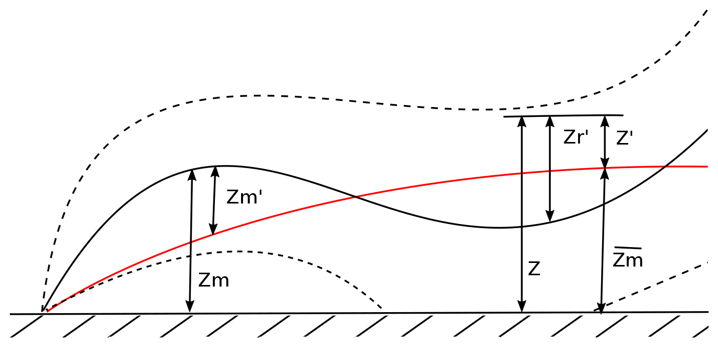
Figure 4 Scheme of an idealized plume dispersing from a ground point-source. Shown here are the mean position of the instantaneous plume z_m and the centerline position as well as the total mean of centerline positions $\stackrel{\mathrm{‾}}{z_m}$ (red line). Also shown are the displacements of particles in the instantaneous plume from its centerline position $z_r^{\prime }$ and from the total mean centerline position z^′ as well as the displacement of the instantaneous centerline from the total mean centerline $z_m^{\prime }$.

4 Results

4.1 Validation of modeled meteorological conditions with available data

Figure 5 shows multiple instantaneous x–y cross-sections of the simulated plume from the realistic simulation. The cross-sections have been taken at 3 m above the ground, i.e., the inlet height on the vehicle used during the campaign (Fig. 1a). It can be seen that the variation of the plume direction is pronounced throughout the simulation. This behavior is caused by very low mean wind speeds that change direction frequently in the simulated turbulent flow field. As was demonstrated in Sect. 2, the large-scale wind and temperature fields showed no pronounced gradients above the area on the simulated day. Therefore, local effects likely governed the flow that was measured at the site. Since ERA5 does not resolve these local effects, the discrepancies between modeled and measured wind are to be expected. To correct for this, the idealized simulation was set up.

Figure 5 Snapshots of instantaneous plumes at 3 m above the surface. Plume at (a) 11:30:00, (b) 12:15:00 and (c) 13:00:00 UTC.

Simulated and nudging profiles for the idealized run are compared in Fig. 3. Note that we replaced the ERA5 wind profiles. The simulated profiles were obtained as spatial averages over the whole domain that were time averaged over 1 h. Throughout the run, θ_l and q_t show very good agreement with the ERA5 profiles. The profiles show hardly any variability over time and are constant with height in the lower ≈ 700 m. This indicates that the spin-up time of the run was sufficiently long for the development of a well-mixed boundary layer. The u wind profile in the idealized run shows virtually no variation. A well-mixed layer above the surface is clearly visible, with stronger and constant winds above 700 m, which correspond to the nudging profiles, and a logarithmic decline towards the surface. The simulated v profiles agree with the imposed zero nudging profiles.

Figure 6a shows the measured CH₄ and N₂O plumes. The plumes in the figure are shown with the background subtracted. Background subtraction follows the procedure described in Ruckstuhl et al. (2012). To help with the interpretation of the plumes, N₂O was released from a cylinder 20 cm above the well head with a constant rate of (0.59 ± 0.02) g s⁻¹ for the duration of the measurements.

The measured horizontal wind speed (Fig. 6b) was low during the whole day, varying from 0.8 to 2.8 m s⁻¹ (1 min averages) during the measurements. A weak periodicity of approximately 55 min can be noticed in the wind speed data. It is possible that it is caused by influences from the local orography, since the area is in the vicinity of hills. The closest elevated area is about 5 km away towards the west (W), and higher mountains are located approximately 10 km towards the N and NW. It was shown in the work of Nastrom et al. (1987) that the mountains can have a considerable effect on atmospheric variability on scales of 4 to 80 km. To verify the possible influence of the mountains in this case, however, the wind data measurements should be considerably longer. The observed periodicity is not present in the simulated wind (Fig. 6b). This is caused by the imposed flat orography in the domain and the constant wind forcing through the nudging on the lateral boundaries. If the surrounding hills would be included in the simulation, fluctuations in the wind direction would likely be simulated. However, the high-resolution domain would have to be expanded far beyond the measurement site. With the current computing resources, this endeavor is unfeasible. In our restricted domain, the simulated and measured wind speeds show good agreement. This is also visible in the 1 min averages of the instantaneous wind direction (Fig. 6c). Since the mean wind direction in the idealized simulation was set to be easterly, the wind was rotated to match the mean wind direction from the observations. It can be seen that the wind angle in the idealized simulation fluctuates comparable to the observations. The standard deviation in wind direction was ${\mathit{\sigma }}_{\mathrm{WD},\mathrm{obs}}=\mathrm{16.9}$^∘ for the measured wind and ${\mathit{\sigma }}_{\mathrm{WD},\mathrm{LES}}=\mathrm{18.6}$^∘ for the simulation.

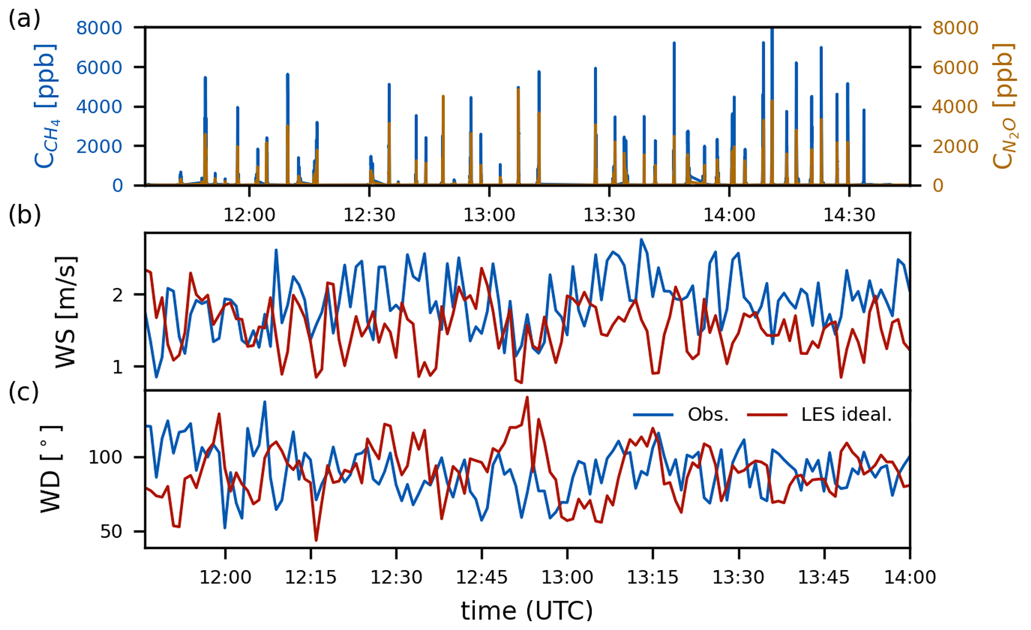
Figure 6 (a) CH₄ molar fractions measured over the road adjacent to the emitting oil well and N₂O molar fractions from emissions next to the well. Comparison of the observed and simulated (b) horizontal wind speed and (c) horizontal wind direction. The values are given as 1 min averages of instantaneous wind. The dotted lines are rolling means of respective wind speeds, shown here for easier interpretation of the mean wind speed.

4.2 Comparison of modeled and measured plume characteristics

Time-averaged plumes from the measurements are given in Fig. 7. The measured plumes were averaged over half-hour increments, and they are shown here together with the mean wind speed and direction for the corresponding time period. The mean horizontal wind direction did not change significantly during the measurement period, except for the first half hour, which deviates by ≈ 40^∘. The mean wind speed for the whole period was low and did not exceed 2.4 m s⁻¹. Since the measurements were collected on a public road, the number of averaged plumes varies from one half-hourly period to another. The number of plumes per half-hourly time period amounts to $n=[\mathrm{3},\mathrm{6},\mathrm{8},\mathrm{4},\mathrm{9},\mathrm{10}]$ starting from 11:30 until 14:30 UTC.

On the right-hand panel of Fig. 7, the corresponding time-averaged simulated plumes are shown. Transects through the plume were sampled according to the observations: at 3 m height and 80 m downwind from the source. Plume transects were taken every 1 min, resulting in 150 transects for the entire simulation. After 14:00 UTC the surface flux of sensible heat turns negative, and that is when the simulation stops. For that reason, the set of time-averaged plumes from LES contains one less element than the measurement set. The half-hour averages of the simulated plumes are smoother compared to the corresponding measured plume averages. This follows from comparing the average skewness of the mean plumes defined as $S=\frac{\mathrm{1}}{\stackrel{\mathrm{‾}}{x_{\max }}N}\left({\sum }_{i=\mathrm{1}}^N\right(x_i-\stackrel{\mathrm{‾}}{x}{)}^{\mathrm{3}}{)}^{\mathrm{1}/\mathrm{3}}$, where x is the half-hour average from either measurement or simulation, $\stackrel{\mathrm{‾}}{x}$ is the mean value of that half-hour average, N in the number of averages and $\stackrel{\mathrm{‾}}{x_{\max }}$ is a maximum value of the total mean plume (red line in Fig. 7). As a result, the LES, CH₄ and N₂O measurements have an average skewness of S_LES=0.32, $S_{{\mathrm{CH}}_{\mathrm{4}}}=\mathrm{0.44}$ and $S_{{\mathrm{N}}_{\mathrm{2}}\mathrm{O}}=\mathrm{0.42}$. The smoother averages in the LES are likely caused by the fact that the number of plumes averaged per half-hour increment is much lower in the measurements compared to the simulation.

The angle over which the wind direction varies during the simulated period amounts to 18^∘, with the exception of the last half-hourly period, in which the wind direction deviated from the mean by ≈ 50^∘.

We used Eq. (1) to infer the unknown CH₄ emission rate from the oil well using the LES plume as the reference. To this end, we compare the time-averaged measured CH₄ plume from the oil well (red line in Fig. 7b), combined with the measured mean horizontal wind speed ($\stackrel{\mathrm{‾}}{u_{\mathrm{meas}}}=\mathrm{1.93}$ m s⁻¹), to the corresponding flux of the time-averaged LES plume (red line in Fig. 7c), combined with the simulated wind speed ($\stackrel{\mathrm{‾}}{u_{\mathrm{ref}}}=\mathrm{1.72}$ m s⁻¹). This leads to the estimated emission rate of $Q_{\mathrm{estim},{\mathrm{CH}}_{\mathrm{4}}}=$ (1.11 ± 0.34) g s⁻¹. Using the same principle, we estimate an N₂O emission rate of $Q_{\mathrm{estim},{\mathrm{N}}_{\mathrm{2}}\mathrm{O}}=$ (0.53 ± 0.15) g s⁻¹ (true emission strength was $Q_{{\mathrm{N}}_{\mathrm{2}}\mathrm{O}}=$ (0.59 ± 0.02) g s⁻¹). To benchmark the performance of LES in this experiment, we also estimate the unknown CH₄ source using the N₂O gas as reference, and we obtain an emission rate of $Q_{\mathrm{estim},{\mathrm{CH}}_{\mathrm{4}}}=$ (1.23 ± 0.12) g s⁻¹. Note here that the standard deviations have been calculated using the source strength estimation from the half-hour averages. The discrepancies between both methods can have various reasons. Firstly, even though the mean wind in the LES is very close to the measured mean wind, their magnitudes and variations are not identical, which can also contribute to the error. However, the most notable cause for the estimation error might arise from the averaging time of the measurements, which is likely too short. It can be observed from Fig. 7 that the time-averaged plumes are not Gaussian shaped, which indicates that turbulent eddies of various sizes still influenced the time averages. The deviation from the normal distribution can be estimated using the Shapiro–Wilk test (Shapiro and Wilk, 1965), and the p values are calculated as p= [9 × 10⁻⁶, 6 × 10⁻¹⁶, 1 × 10⁻¹⁶] for the LES, CH₄ and N₂O plumes, respectively. Therefore, the measured plumes deviate from the expected Gaussian profile and are not as smooth as the LES plume due to the much smaller set of plumes being averaged. Nevertheless, this analysis shows that LES is a useful tool in source estimation in real-atmosphere conditions, e.g., in cases for which the source location is inaccessible for a tracer release.

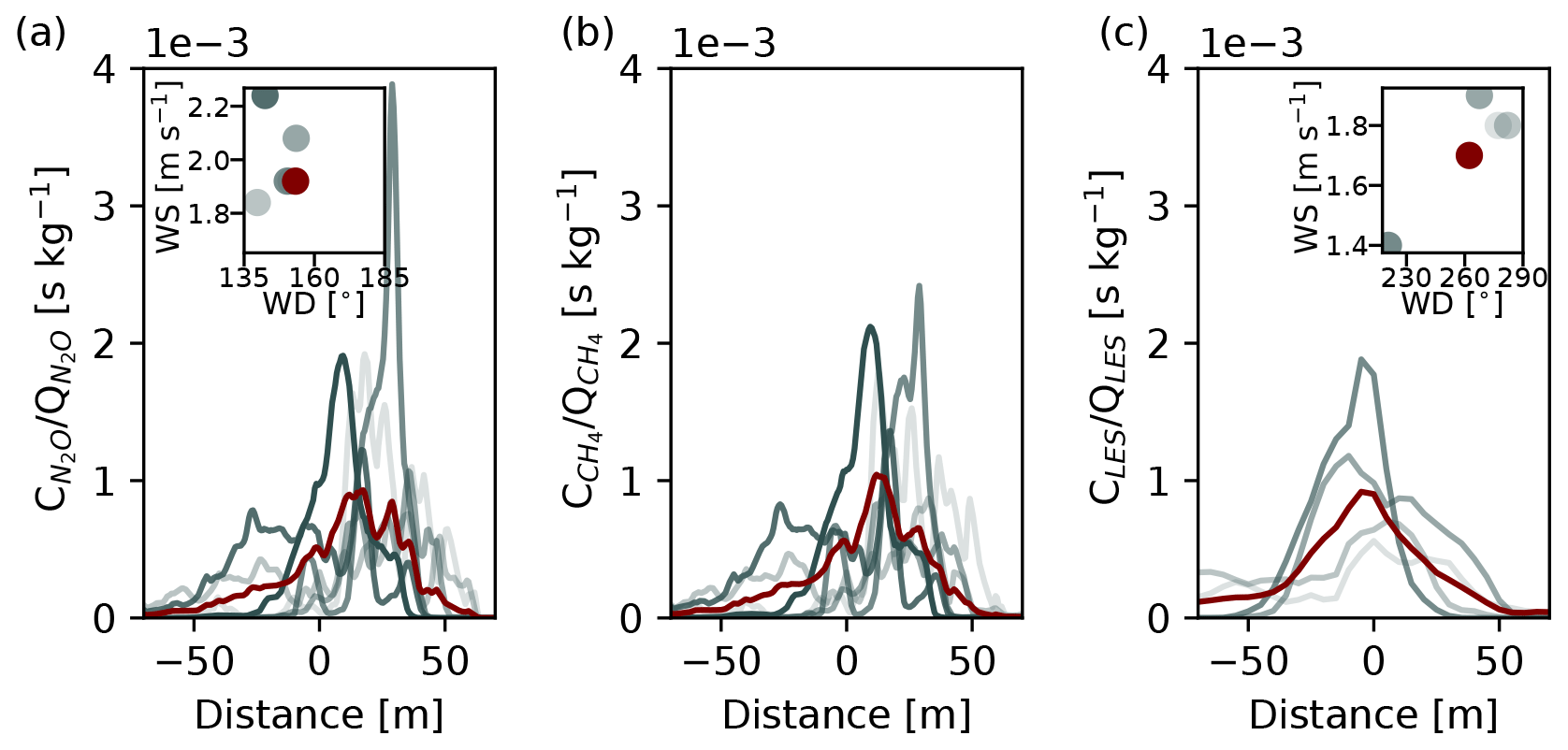
Figure 7 Averages of instantaneous plumes over half-hour periods from (a) N₂O, (b) CH₄ and (c) LES. All plumes have been scaled with their respective emission rates, i.e., $Q_{{\mathrm{N}}_{\mathrm{2}}\mathrm{O}}=\mathrm{0.59}$, $Q_{{\mathrm{CH}}_{\mathrm{4}}}=\mathrm{1.23}$ and Q_LES=1 g s⁻¹. LES transects were taken at 3 m height and 78 m downwind from the source. Plumes are shown with a color gradient corresponding to the half-hour increments i.e., lightest gray plume is the average of plumes measured over the time period 11:30–12:00 UTC; dark gray is the average over 14:00–14:30 UTC. The inset shows horizontal wind speed and direction for the corresponding half-hour averages in (a) measurements and (c) LES. Overlaid in red is the average of all the plumes, as well as the averages of horizontal wind speed and direction in the insets.

4.2.1 Absolute dispersion

In this section, we analyze the general behavior of the LES plume through its first three statistical moments i.e., the center of mass, width of the plume and skewness. As shown in the previous section, the typical mobile plume measurements consist of a relatively small number of 1D plume transects. While such measurements might be well suited for inferring the unknown source strength, we aim here to exploit LES further. We will do this by linking the simulated plume to previous, more idealized, plume dispersion studies. First we focus on the absolute motion of the plume with respect to the ground surface, and we will statistically analyze plume dispersion due to plume meandering and due to motions relative to the plume center of mass. In a later stage, we will separate the two, as described in Sect. 3.3, and analyze the contribution of the two processes separately.

Figure 8 shows instantaneous and time-averaged plumes (averaged over 105 time steps). The plumes were integrated over depth (x–y transect) and width (x–z transect). Clear differences in the structure of the plume can be observed between the instantaneous and time-averaged shape. Firstly, the top view on the time-averaged plume (panel b) shows a clear Gaussian shape as expected, which deviates from the instantaneous plume shown in panel (a). In the instantaneous plume, eddies of different sizes influence the plume throughout. The integrated x–z transect of the plume shows more complex behavior. The solid line in the bottom panel of Fig. 8 shows the mean of all centerline plume positions as defined by Eq. (2). In contrast, the dotted line denotes the position of the maximum concentration of the integrated x–z plume. Firstly, it can be noticed that the positions of the maximum and the mean do not coincide close to the source (x<2500 m), while at large distances the two lines tend to converge. Secondly, the position of the maximum concentration is located at the ground level for x<2000 m. For larger distances, the maximum concentration moves towards the top of the boundary layer, and a local minimum is visible at the surface. Dosio and de Arellano (2006) performed a turbulent channel flow study with a similar setup as we presented here. They presented their results as a function of the normalized distance x_*, defined as the following:

$$\begin{array}{}\text{(8)}& x_{*}={\displaystyle \frac{w_{*}}{h_{\mathrm{BL}}}}{\displaystyle \frac{x}{\stackrel{\mathrm{‾}}{u}}},\end{array}$$

where w_* is the convective velocity scale, h_BL is the height of the boundary layer, x is the distance from the source and $\stackrel{\mathrm{‾}}{u}$ is the mean wind speed over the whole domain. Intuitively, this distance quantifies the number of overturns of the largest eddies (convective timescale $T_M=\frac{h_{\mathrm{BL}}}{w_{*}}$) at distance x from the source (advective timescale $T_{\mathrm{A}}=\frac{x}{\stackrel{\mathrm{‾}}{u}}$). Dosio and de Arellano (2006) reported similar behavior in the mean of their plume emitted from an elevated source. In that simulation the concentration maximum was first transported towards the surface and later lifted towards the boundary layer top. The corresponding local minimum at the surface occurred at $x_{*}=\mathrm{1.75}$. In our simulation, it was with $w_{*}=\mathrm{0.94}$ m s⁻¹, $\stackrel{\mathrm{‾}}{u}=\mathrm{2.64}$ m s⁻¹, and h_BL=564.64 m. Here, the boundary layer height was calculated as the maximum of the domain- and time-averaged vertical profile of the potential temperature gradient. The minimum occurs at $x_{*}=\mathrm{1.9}$, which is in good agreement with the results by Dosio and de Arellano (2006). As mentioned previously, the position of the concentration maximum converges to the plume centerline position at larger distances from the source. This result, however, differs from the results reported by Dosio and de Arellano (2006). In their simulation, the plume never reaches a well-mixed state, which was in agreement with water tank experiments performed by Willis and Deardorff (1978), who reported well-mixed plume only at very large distances from the source at $x_{*}=\mathrm{6}$. In comparison, in our simulation the maximum of concentration starts approaching the mean plume position at $x_{*}\approx \mathrm{2.5}$. The instantaneous plume we show here (Fig. 8c) has stayed close to the ground for ≈ 1500 m from the source, after which it gets mixed in with larger-sized eddies towards the top of the boundary layer. Additionally, puff-like structures with higher concentrations can be observed, which have been lifted from the ground and are carried to the top of the BL even at large distances from the source (e.g., x=3000 m).

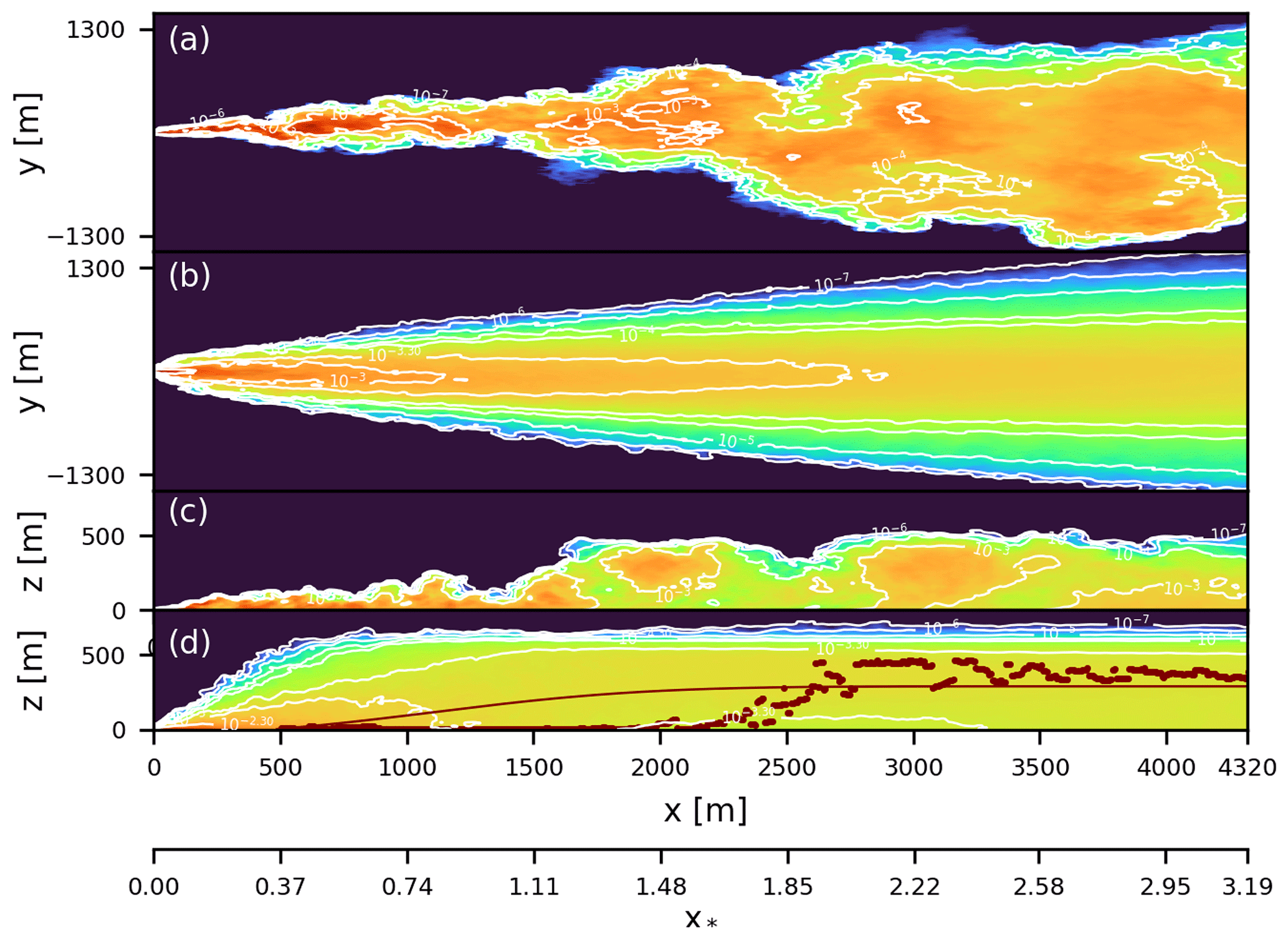
Figure 8 Top view of vertically integrated (a) instantaneous and (b) time-averaged plumes. Horizontally integrated (c) instantaneous and (d) time-averaged plume. Also shown in panel (d) are mean plume centerline position (solid red line) and position of the maximum of concentrations (dotted red line). x_* is the normalized distance from the source as defined in Eq. (8).

Figure 9 shows the first three statistical moments of the plume. The top two panels show the plume centerline position in the y and z directions, downwind from the source. The centerlines of the instantaneous plume positions in y direction show large variability throughout the domain. However, the mean center of mass is constant and centered at the y position of the source. In contrast, the centerline position of the plume in the z direction changes drastically downwind from the source and stabilizes at approximately 300 m height at 1500 m from the source. As the plume gets mixed through the boundary layer, the variability in the plume centerline positions drops. Thus, while in the y direction the plume keeps growing throughout the domain, the growth stops in the z direction once the plume reaches the top of the boundary layer (Fig. 9c, d). The skewness of the plume positions (Fig. 9e) shows that the plume is oscillating around its mean value in the y direction. In the vertical direction, however, the instantaneous plumes are more likely to have their centerline position below the mean plume centerline in the first 1500 m from the source ($\stackrel{\mathrm{‾}}{S_{za}}>\mathrm{0}$).

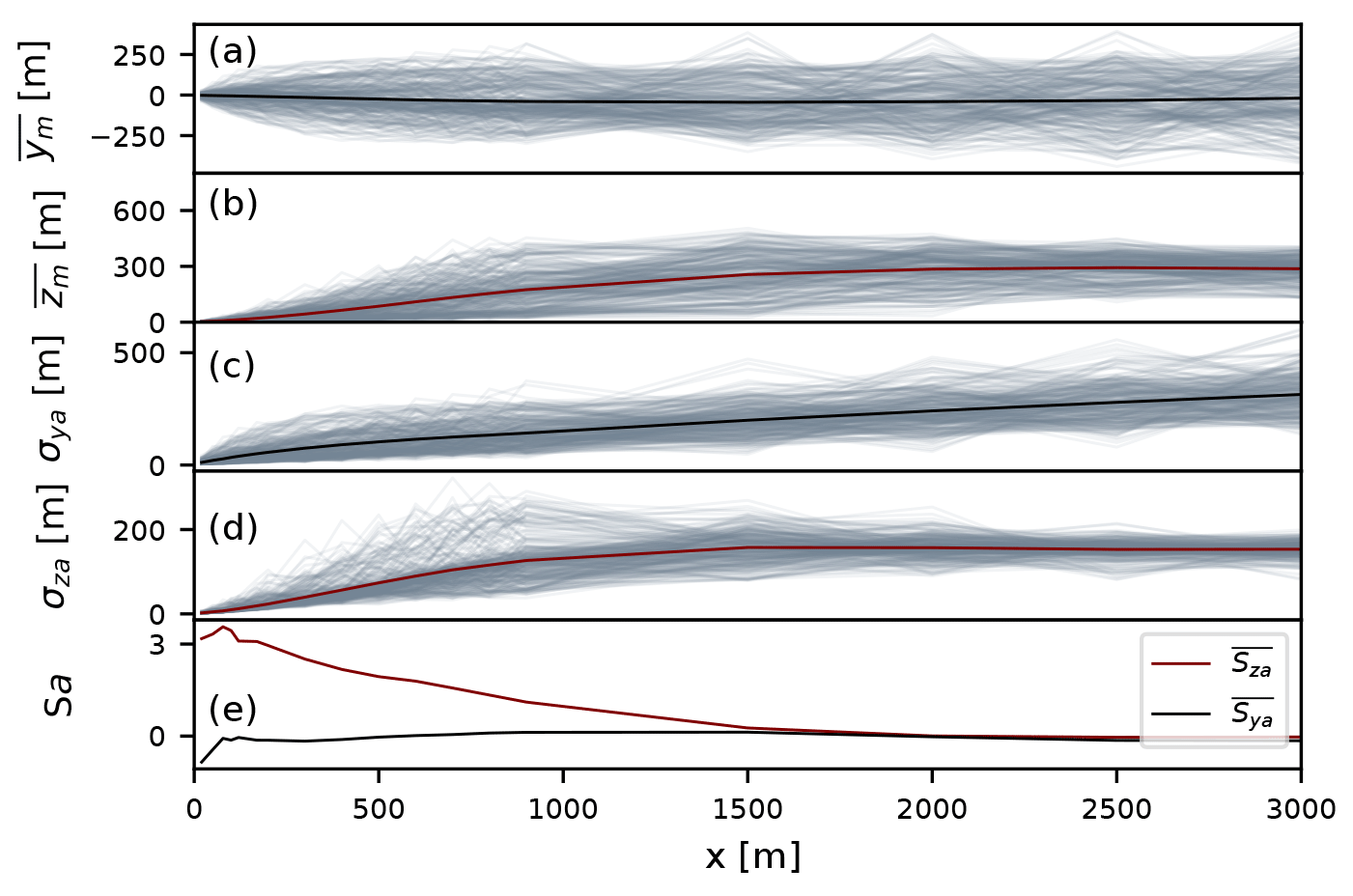
Figure 9 The first three statistical moments of the simulated plume in the absolute coordinate system. The first four panels show position of the center of mass in y and z directions and the plume width in the y and z directions. All values are shown as a function of downwind distance x. Gray lines denote instantaneous plumes, and mean values are shown as solid black and red lines in y and z directions, respectively. The bottom panel shows the skewness of the mean centerline plume position as a function of distance from the source.

To inspect the skewness of the plume more closely, Fig. 10 shows probability density functions (pdfs) of center of mass positions in the y and z directions around their mean values at various downwind distances. As already noted in discussing Fig. 9, in the y direction the plume positions show a Gaussian distribution on all distances from the source. Note that the spread of the centerline positions grows with distance from the source, indicating that the plume gets moved further away from the mean centerline position with bigger and bigger eddies. This Gaussian distribution of the plume centerline position was also found in previous studies. For instance, Gailis et al. (2007) assumed a Gaussian distribution of the plume centerline position for their fluctuating plume model, which they experimentally confirmed in a water channel experiment. In contrast, close to the source, the centerline position distribution in the z direction is positively skewed. A Gaussian distribution is attained further downwind. This result differs somewhat from previous studies (Gailis et al., 2007; Marro et al., 2015), in which lognormal and reflected Gaussian distributions were assumed for modeling the plume vertical mean position. We show here that, only close to the source, the lognormal distribution provides a good description of the centerline positions. Further downwind, where the plume gets better mixed in the convective boundary layer, the centerline position starts oscillating around its mean position.

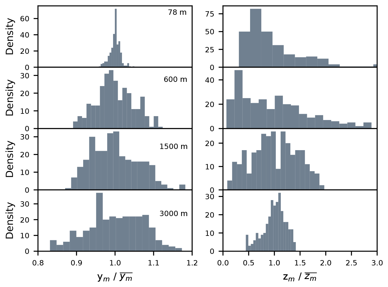
Figure 10 Probability density functions of the instantaneous plume position scaled with the mean centerline position at various downwind distances from the source.

4.2.2 Relative dispersion

There are two processes that affect plume growth: meandering motions (discussed in the previous section) and relative dispersion due to mixing by small eddies. Understanding these two processes (and quantifying where a certain process is dominant) can aid the development of measurement strategies. For example, at downwind distances where relative dispersion dominates, the instantaneous plumes remain close to the mean position, and the chance of measuring the plume close to its centerline increases.

Firstly, we focus on the relative dispersion. Relative dispersion is defined as dispersion of the plume around its centerline due to the eddies of comparable size or smaller than the plume. We present second- and third-order statistics of relative plume dispersion in Fig. 11 (left column). Close to the source, the contribution of relative dispersion to the total plume growth is still small, which is especially visible in the y direction (Fig. 11 a). As the plume moves away from the source, it grows in size. This enables bigger and bigger eddies to be involved in the mixing of the plume (Cassiani et al., 2020). For this reason, the size of the plume due to relative dispersion is growing downwind from the source at a constant rate. Similar behavior is seen for dispersion in the z direction. Close to the source, the contribution of relative dispersion is small and it grows further downwind. Unlike the z direction, in which the plume growth is limited by the size of the BL, the growth of the plume in the y direction is unrestricted by boundaries. This implies that the plume growth will continue until the plume is so dispersed that it becomes indistinguishable from the background concentrations. The skewness of the relative plume dispersion in the z direction shows a positive value close to the source, which can be attributed to plume reflection at the surface. Since the small turbulent motions that are responsible for relative dispersion are random and Gaussian in nature, the asymmetry has to originate from the fact that the plume is close to the surface (Dosio and de Arellano, 2006). In the y direction, the plume shows virtually no skewness.

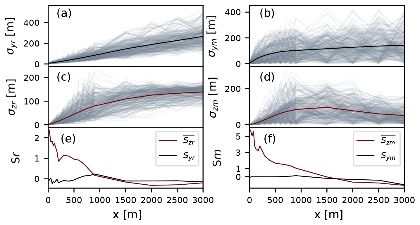
Figure 11 The second- and third-order moments of the simulated plume for the relative (a, c, e) components centered around the mean plume position and for the meandering (b, d, f) components. The first two panels in a row show the plume width in the y and z directions. All values are shown as functions of downwind distance. In gray are shown values of instantaneous plumes while their mean values are shown as solid black and red lines in y and z directions, respectively. The last panel shows skewness of the mean relative plume position as a function of distance from the source.

4.2.3 Meandering

Finally, we look at the plume dispersion due to the meandering of the plume, i.e., displacement of the plume caused by the eddies that are larger than the plume itself. Figure 11b, d and f show the second and third moments of the plume due to the meandering motions. It can be observed that in the y direction the plume shows large symmetric growth very close to the source (Fig. 11b). The magnitude of the meandering component in this region is up to 2.5 times larger than the relative dispersion (Fig. 11a). However, while the relative contribution continues to grow further downwind, the growth due to meandering drops significantly and becomes almost constant. This observation is in line with the theoretical analysis given in Csanady (1973), where y scaling was reported according to σ_ym=σ_vt (where σ_v is the variance of the v component of velocity, and t is the time since the plume left its source) close to the source, and $\frac{d{\mathit{\sigma }}_{ym}}{\mathrm{d}t}=\mathrm{0}$ far from the source. This was later confirmed in the water tank experiment by Weil et al. (2002), and the LES study presented by Dosio and de Arellano (2006). Our results agree well close to the source. However, in our simulation there are still eddies big enough to move the whole plume even farther downwind, since our value of σ_ym does not become fully constant. In contrast, the contribution of meandering to the total dispersion in z direction tends to zero further downwind from the source. The size of the eddies that develop in the vertical direction is constrained by the depth of the boundary layer. For this reason, with only meandering, the plume attains a size comparable to these eddies.

The distance at which the relative regime becomes predominant can be estimated from the relevant convective and advective timescales introduced in Sect. 4.2.1. When the two timescales become equal, the plume has spent enough time in “flight” to be mixed with the largest eddies. Therefore, a length scale, L_mix, can be derived that defines the downwind distance at which the plume starts to be mixed with eddies of all sizes and at which the relative dispersion becomes predominant:

$$\begin{array}{}\text{(9)}& L_{\mathrm{mix}}={\displaystyle \frac{\stackrel{\mathrm{‾}}{u}{h}_{\mathrm{BL}}}{w_{*}}}.\end{array}$$

In this study, this distance amounts to L_mix= (1360 ± 68) m. L_mix in this case is an average of the values for the mixing distances calculated every 300 s. Alternatively, this distance can be obtained from the meandering ratio $M\equiv {\mathit{\sigma }}_{im}/{\mathit{\sigma }}_{ir}$, where $i=y,z$ (Oskuie et al., 2015). When M drops to values smaller than 1, the relative dispersion becomes the dominant process. This occurs at x ≈ 1320 m downwind of the source, which is in good agreement with the estimated length scale. Note that this distance is specific for each case. It depends not only on the turbulence regime and the BL height but also on the release height.

4.3 Concentration statistics

Finally, we will present concentration statistics in the absolute and relative coordinate systems. Additionally, we will compare these statistics to parametrizations that are commonly used in fluctuating plume models (Gailis et al., 2007; Marro et al., 2015; Cassiani et al., 2020). These fluctuating plume models have been validated against dispersion studies in laboratory channel flows, often by taking line transects through the plume (e.g., Nironi et al., 2015). Here we aim to utilize the high spatial and temporal resolution of LES to estimate dispersion parameters, needed in these models. Figure 12 (first and second row) shows y–z transects through the time-averaged plume (average of 287 instantaneous plumes) in the absolute (left) and relative (right) coordinate systems. In the relative system, the instantaneous plumes were aligned with the center of mass of the mean plume ($\stackrel{\mathrm{‾}}{y_m}$, $\stackrel{\mathrm{‾}}{z_m}$). It can be seen that close to the source (top row) the two plumes are similar in shape since the maximum of concentration and centerline position still coincide. Further downwind, there is a clear difference between the plumes since the plume entered the regime in which it was more frequently carried upwards by strong ejections (see e.g., Fig. 10). For the distances furthest downwind (Fig. 12, bottom row), the two plumes again attain similar shapes. Here, the relative dispersion is the dominant mechanism, and the centerlines of the instantaneous plumes do not move far from its mean position by meandering motions. For the two distances closer to the source, the edges of the plumes show large variability, despite the large number of plume transects that was used in time-averaging. This is caused by the plume behavior. Close to the source, the plume tends to stay close to the ground. The large spatial variability away from the ground is caused by occasional ejections by strong upwards motions. Further downwind, the plumes attain a more uniform shape, resembling a Gaussian distribution.

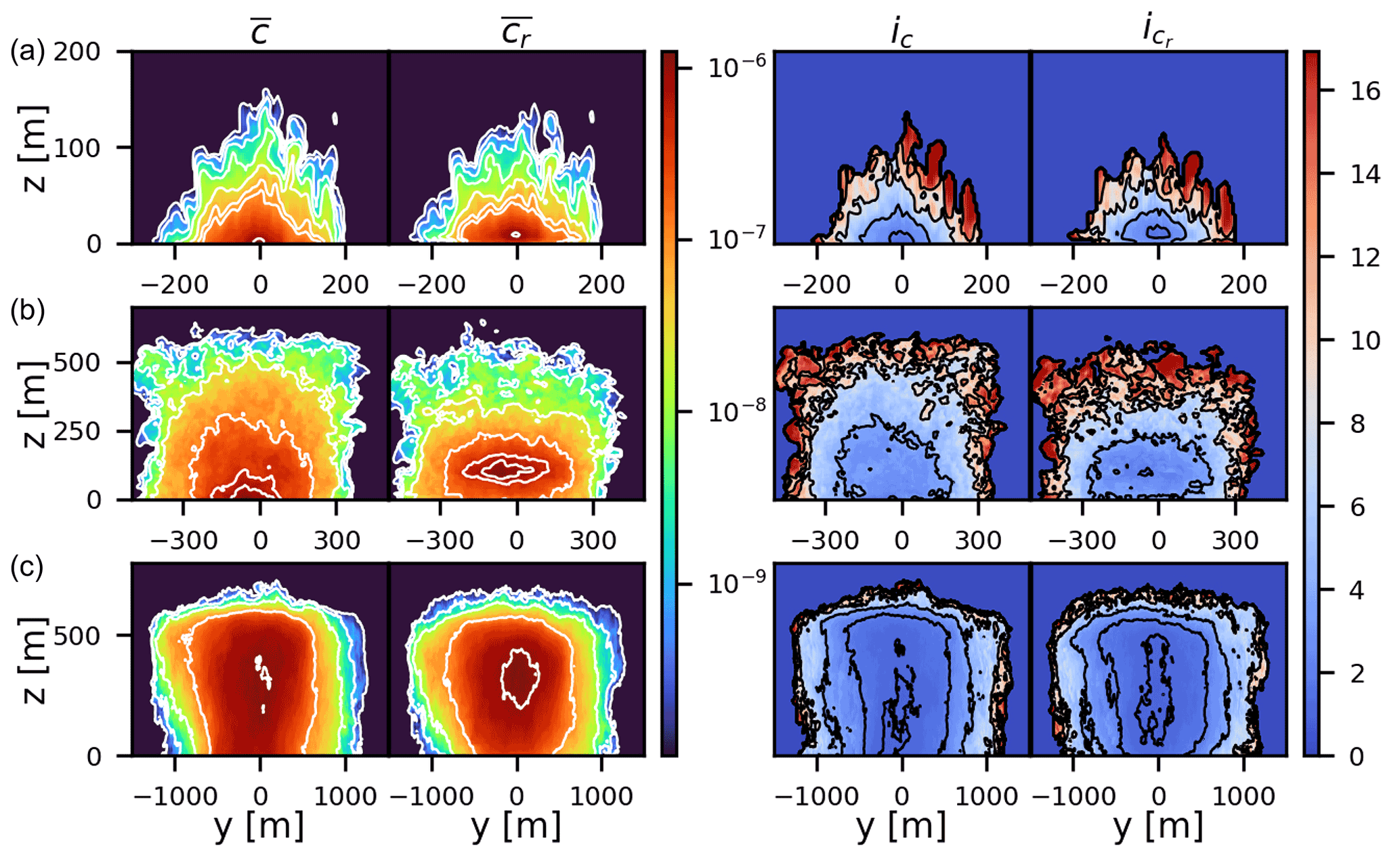
Figure 12 First two columns: y–z transect of mean plume concentrations in absolute ($\stackrel{\mathrm{‾}}{c}$) and relative ($\stackrel{\mathrm{‾}}{c_r}$) coordinate systems. Last two columns: concentration fluctuation intensity in y–z plume in absolute (i_c) and relative (i_cr) coordinate systems. Distances from the source are (a) 100, (b) 600 and (c) 3000 m.

4.3.1 Parametrization of concentration fluctuations intensity

One of the commonly used parameters to model the concentration pdf is the concentration fluctuation intensity, defined as $i_{\mathrm{c}}=\frac{{\mathit{\sigma }}_{\mathrm{c}}}{\stackrel{\mathrm{‾}}{c}}$ (Gailis et al., 2007; Nironi et al., 2015; Cassiani et al., 2020), with $\stackrel{\mathrm{‾}}{c}$ being the mean concentration (x of plumes averaged) and σ_c its standard deviation. As pointed out in Marro et al. (2015), the spatial evolution of this non-dimensional parameter is often assumed to depend only on the x coordinate. This can lead to significant discrepancies between modeled and measured concentration fields. We use LES to demonstrate the complex spatial structure of variable i_c, both in absolute and relative coordinates, over a plume crosswind transect (Fig. 12, third and fourth rows). Close to the plume centerline i_c has minimum value, but it increases noticeably towards the plume edge. This is most clearly visible close to the source. In the far field, these differences are less pronounced, which is a consequence of the plume being better mixed, which decreases the intermittent behavior.

Furthermore, from a measurement point of view, knowledge of the shape of i_c can help in planning the measurement campaigns. High values of i_c imply that the probability of measuring the plume in that area is lower, and longer measurement times are required to achieve reliable plume statistics. Knowledge of the optimal downwind distance and height at which to measure can considerably improve the efficiency of the measurement process.

The measurements used in this study were taken as line transects at a single height (3 m). According to the results presented here, at 3 m height the plume was the least fluctuating very close to the source (x ≲ 300 m) and in the far field (x ≳ 1500 m). We have previously shown that in the near field the pdf of vertical centerline position is positively skewed (Fig. 10 right row); therefore, there was higher likeliness of capturing the plume closer to the ground than at its centerline. Conversely, far from the source, the plume is oscillating around its centerline, and there is the highest chance of measuring the plume. In the mid-field (300 ≳x≲ 1500 m), the plume is highly oscillating at the ground and at the centerline position, but since it is still positively skewed, there is a higher chance of measuring the plume at the ground.

The complex 3D structure of i_cr has been addressed in previous studies. Marro et al. (2015) expanded upon the definition of i_cr given in Gailis et al. (2007), where the relative concentration fluctuation has been expressed in terms of the mean relative concentration field. The model presented in Marro et al. (2015) is given as the following:

$$\begin{array}{}\text{(10)}& \begin{array}{rl}{i}_{\mathrm{cr}}^{\mathrm{2}}=& {\left(\mathrm{1}+i_{\mathrm{cr}\mathrm{0}}\right)}^{\mathrm{2}}\mathit{\left\{}\exp \right[-{\displaystyle \frac{{\left(y-y_m\right)}^{\mathrm{2}}}{\mathrm{2}{\mathit{\sigma }}_{yr}^{\mathrm{2}}}}]{\mathit{\}}}^{-{\mathit{\zeta }}_y\left(x\right)}\\ & \times \mathit{\left\{}\exp \right[-{\displaystyle \frac{{\left(z-z_m\right)}^{\mathrm{2}}}{\mathrm{2}{\mathit{\sigma }}_{zr}^{\mathrm{2}}}}]\\ & +\exp [-{\displaystyle \frac{{\left(z+z_m\right)}^{\mathrm{2}}}{\mathrm{2}{\mathit{\sigma }}_{zr}^{\mathrm{2}}}}]{\mathit{\}}}^{-{\mathit{\zeta }}_z\left(x\right)}\\ & \times \mathit{\{}\mathrm{1}+\exp [-{\displaystyle \frac{{\left(\mathrm{2}{z}_m\right)}^{\mathrm{2}}}{\mathrm{2}{\mathit{\sigma }}_{zr}^{\mathrm{2}}}}]{\mathit{\}}}^{-{\mathit{\zeta }}_z\left(x\right)}-\mathrm{1},\end{array}\end{array}$$

where i_cr0 is the value of relative concentration fluctuation at the plume centerline (Fig. 13a), and ζ_y(x) and ζ_z(x) are the shape parameters introduced to account for anisotropy in the y and z directions. The variables that determine the crosswind shape of i_cr (y_m, z_m, σ_yr and σ_zr) need to be either determined from plume measurements or parameterized using one of the models (e.g., Gailis et al., 2007; Marro et al., 2015). Here they are calculated from the LES data as defined in Sect. 3.3. The two ζ functions were assumed to be sigmoid, such that the modeled i_cr has value i_cr0 close to the source and has self-similar profiles in the far field in both y and z directions. As previously mentioned, the LES data show the U-shaped profile in the far field but also close to the source (not shown). This is likely caused by the fact that in the simulation the source is not introduced as point source, as assumed in the plume model, but as a 2D Gaussian in the x and y directions with 1 standard deviation the size of one grid box ($\mathrm{\Delta }x=\mathrm{\Delta }y={\mathit{\sigma }}_{\mathrm{source}}=\mathrm{5}$ m). Therefore, 95 % of mass is being emitted from an area that has a horizontal transect of 20 m. The size of the smallest eddies that can develop in the simulation is ≈ 4Δx. This means that very close to the source there is no internal mixing in the plume by the smaller eddies, and all of the fluctuations are caused by entrainment of ambient air by eddies comparable in size to the plume.

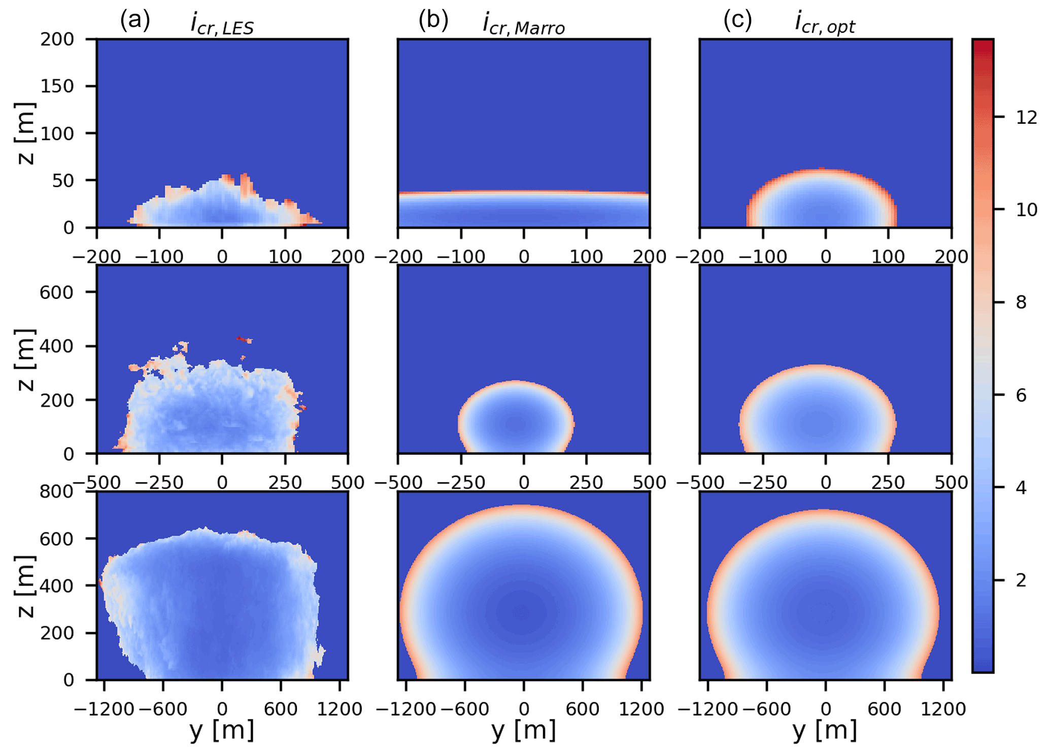
We have adapted the definition of the shape functions ζ given in Marro et al. (2015) to account for the shape of the source in the near-field y direction and kept the same behavior in the far field. The far field was defined as the distance at which the relative dispersion becomes dominant, i.e., at the characteristic length scale L ≈ 1360 m (Sect. 4.2.3). The slope of the sigmoid function β, which defines the shape of functions ζ, was determined using L. It was assumed that at distance L from the source the value of ζ has p % (here we used p=70 %) of the amplitude defined in Marro et al. (2015). p was chosen as the ratio of relative to absolute dispersion for the respective directions at the distance L. As a result, the functions take the following shape:

$$\begin{array}{}\text{(11)}& \begin{array}{rl}& {\mathit{\zeta }}_y=\mathit{\gamma }+{\displaystyle \frac{{\mathit{\alpha }}_y-\mathit{\gamma }}{\mathrm{1}+\exp \left[-{\mathit{\beta }}_y(x-x_{\mathrm{0}})\right]}},\\ & {\mathit{\zeta }}_z={\displaystyle \frac{{\mathit{\alpha }}_z}{\mathrm{1}+\exp \left[-{\mathit{\beta }}_z(x-x_{\mathrm{0}})\right]}},\end{array}\end{array}$$

where γ=2 × 10⁻³ is the correction for the shape of the source, α_y=0.45 and α_z=0.9 are the amplitudes taken from Marro et al. (2015), x₀=0.5 L is the location of the function's midpoint, and the slopes are calculated as

$$\begin{array}{}\text{(12)}& {\mathit{\beta }}_y=-{\displaystyle \frac{\mathrm{2}}{L}}\ln \left({\displaystyle \frac{(\mathrm{1}-p){\mathit{\alpha }}_y}{p{\mathit{\alpha }}_y-\mathit{\gamma }}}\right),{\mathit{\beta }}_z=-{\displaystyle \frac{\mathrm{2}}{L}}\ln (\mathrm{1}-p).\end{array}$$

Figure 13 shows the comparison of i_cr calculated from the LES data and i_cr modeled with the two definitions of the ζ function. As previously mentioned, the definition of ζ found in the literature (Marro et al., 2015) agrees well with the LES-calculated relative fluctuations in the far field. Very close to the source, the LES plume has a similar structure as in the far field, which is not accounted for when the assumption of constant valued i_cr is made. When the correction for the source shape is added (Eq. 11), the i_cr model represents the plume behavior well, both in the far field and close to the source. It should be noted here that the plume behavior at distances from the source where meandering is important is still misrepresented by the plume model.

One of the assumptions in the meandering plume model is that the relative dispersion and the fluctuations of the instantaneous center of mass are statistically independent processes. This assumption is violated when the size of the plume is comparable to the average size of eddies in the domain. In this case, the eddies that are capable of moving the center of mass of the instantaneous plume are still small enough to entrain ambient air deep into the plume, making the separation of two processes complicated.

Figure 13 The y–z transect of the concentration fluctuation intensity in the relative coordinate system i_cr calculated from the LES data. The other two columns show i_cr calculated with Eq. (10) as found in the literature (b) and optimized for this case (c).

4.3.2 Concentration probability density function

Lastly, we look at the concentration pdf at multiple in-plume locations. A large number of studies have found the gamma distribution to be an appropriate description for the pdf of relative concentrations in the far field (e.g., Dosio and de Arellano, 2006; Nironi et al., 2015; Marro et al., 2015; Cassiani et al., 2020). In the far field, relative dispersion becomes the main mechanism that drives the plume fluctuations. Therefore, the probability of the plume centerline position tends towards a Dirac delta function, and the plume spread due to meandering motions becomes negligible. The pdf can then be expressed as the following:

$$\begin{array}{}\text{(13)}& p={\displaystyle \frac{{\mathit{\lambda }}^{\mathit{\lambda }}}{\stackrel{\mathrm{‾}}{c_r}\mathrm{\Gamma }\left(\mathit{\lambda }\right)}}\left({\displaystyle \frac{c_r}{\stackrel{\mathrm{‾}}{c_r}}}{)}^{\mathit{\lambda }-\mathrm{1}}\exp \right(-{\displaystyle \frac{\mathit{\lambda }{c}_r}{\stackrel{\mathrm{‾}}{c_r}}}),\end{array}$$

where $\mathit{\lambda }=\mathrm{1}/i_{\mathrm{cr}}^{\mathrm{2}}$, and the subscript r denotes the relative plume. Figure 14 shows pdfs of the relative concentration sampled at the plume centerline on multiple downwind distances and, for comparison, at the inlet height at which data presented in Sect. 2.2 were measured. The gamma distribution is indeed a good fit for concentration pdf at the plume centerline for most downwind distances. The mean p value calculated using the Kolmogorov–Smirnov test amounted to 0.26 in the range x= [100, 1500] m downwind from the source. The optimal range of downwind distances where the gamma distribution is the best fit for the pdf has also been found in the LES study by Ardeshiri et al. (2020), where they connected the start of this range with the maximum of i_cr on the centerline. Following the results in Fig. 14, the gamma functions at the inlet height (z=3 m) seem to reasonably fit the concentrations away from the plume centerline. However, the p values obtained from the Kolmogorov–Smirnov test on most downwind distances had values below 0.05, which indicates that the gamma distribution does not provide the best fit in this case. Note that the i_cr that was used here for the calculation of the pdf has been calculated from the LES data. We concluded earlier that the i_cr has a complex structure, which cannot be assumed constant in the y–z plane. When its value is known, either from data or from an appropriate plume model, the pdf of concentration fluctuations can be modeled with a gamma distribution for a certain in-plume location.

Figure 14 Probability density function of concentrations at the plume centerline (a) and at the measurement inlet height (b, see Sect. 2.2) at multiple downwind distances. Overlaid are gamma function fits.

5 Conclusions

Our study aimed to bring together field observations and high-resolution simulations. Large-eddy simulations (LESs) have been employed in dispersion studies for the past few decades but most often simulating dispersion in somewhat idealized settings. The models capable of performing LES are constantly being improved, with higher spatial resolution, and with new parameterizations that include more processes that influence the plume dispersion. We demonstrated here the ability of LES to reproduce plume dispersion in an actual field campaign. We took a step away from idealized channel flows and used available meteorological data to reproduce field conditions encountered during the campaign. Since field observations are sparse, LES can lead to improved understanding in plume behavior, which can help with planning and optimizing future measurement strategies. In particular, LES can aid in understanding which heights the plume centerline can be expected, depending on the downwind distance, and where the plume is expected to be most fluctuating. The latter situation consequently requires a larger number of measurements to average out the atmospheric variability from the mean plume. The case we studied was a methane plume emitted from an oil well that was measured during 1 single day of the ROmanian Methane Emissions from Oil and gas (ROMEO) campaign. The boundary conditions in the LES were derived from ERA5 data (Hersbach et al., 2020) to ensure correct meteorological conditions in the simulation. The plume in the simulation was released from the lower boundary and sampled in accordance with the field observations.

Firstly, the meteorological variables from the LES were compared with the available field data and the ERA5 profiles. The vertical profiles of specific humidity and temperature in ERA5 data showed little variability for the period in which the measurements were taken. The LES was able to reproduce these profiles correctly. There was very little large-scale advection present for the chosen day, which implies that the wind was driven by local temperature differences and orography that are not properly captured with the model resolution of ERA5. This resulted in discrepancies between the LES-generated wind profiles and the measured wind. The issue was circumvented by applying a wind correction and performing a second simulation with this background wind. While the forcing of the boundary conditions with the ERA5 data gave good results, more detailed measurements of meteorological variables (vertical profiles of wind components, temperature, humidity, etc.), together with plume measurements, would help to better evaluate the simulations.

Secondly, the LES was compared with plume observations. A methane plume emitted from an oil well was sampled with an instrument mounted on a moving vehicle. A tracer gas plume emitted close to the oil well was measured simultaneously. The tracer gas plume was used in the estimation of the emission rate from the unknown source. Our aim in this study was to evaluate whether LES can be used as a proxy for the tracer gas. The estimate of the emission rate from the oil well using the tracer gas plume is $Q_{{\mathrm{CH}}_{\mathrm{4}}}=$ (1.23 ± 0.12) g s⁻¹. Using LES, we found $Q_{{\mathrm{CH}}_{\mathrm{4}},\mathrm{LES}}=$ (1.11 ± 0.34) g s⁻¹, i.e., 10 % lower. To further evaluate LES, we estimated the emission rate of the tracer gas ($Q_{{\mathrm{N}}_{\mathrm{2}}\mathrm{O}}=$ (0.59 ± 0.02) g s⁻¹) using the simulated plume, and we found a value of $Q_{{\mathrm{N}}_{\mathrm{2}}\mathrm{O},\mathrm{LES}}=$ (0.53 ± 0.15) g s⁻¹. Part of the differences in the estimated emission rates can be attributed to the different mean wind speeds in the simulation and in the measurements. Nevertheless, it was shown that, using a careful setup of the simulations, LES can replace the co-emitted tracer gas, e.g., in cases of poor access to the source area.

LES provides concentration fields throughout the domain with great temporal and spatial detail. This allows for a more in-depth study of the behavior of the measured plume. The plume was studied by analyzing its absolute position and by separating the processes driving its dispersion into meandering motions of the plume centerline and the relative dispersion around this centerline. A good agreement of the plume behavior was found with previous experimental and theoretical dispersion studies targeting channel flows. Furthermore, a plume-mixing length scale L was derived from the boundary layer height, the mean horizontal wind speed and convective velocity scale. This scale was demonstrated to coincide with the distance from the source at which the relative dispersion becomes the main mechanism of plume growth, and for this case study L= (1360 ± 68) m.

Finally, we used LES to examine parameterizations of concentration fluctuations in simple models: the fluctuating plume model. We did this by focusing on the concentration fluctuation intensity parameter, i_c, an often utilized parameter. LES can provide the detailed 2D fields of i_c, something that is difficult to obtain in laboratory experiments. We confirmed the characteristic U-shape in a horizontal crosswind transect of concentration fluctuation intensity in a relative coordinate system i_cr (Gailis et al., 2007) not only in the far field but also close to the source. We speculate that this is due to spatial extent of the source in the simulation, which is imposed to avoid numerical instabilities. In this way the simulation differs from the field experiments, where close to the source the plume is mixed by eddies ranging from the Kolmogorov scale to the size of the plume itself, making the plume compact and very well mixed. We adapted the semiempirical model for i_cr from Marro et al. (2015) to account for the source shape, and this model showed good agreement with LES.

Furthermore, knowledge of the shape of i_c can help in planning future measurement campaigns, as it is an indication of the chance that the plume will be measured. For the campaign analyzed here, it seems that the plume was measured where there was the highest chance of capturing it – close to the source and the ground. In general, far away from the source the plume is best measured close to its mean centerline, which is likely lifted off the ground as the plume gets mixed throughout the boundary layer. Close to the source, however, the plume is mostly below its centerline, so the chances for measuring it are higher closer to the ground. Following the study by Dosio and de Arellano (2006) of dispersion from an elevated source in a convective boundary layer, it seems that this is true for the lifted sources as well; close to the source most plumes first get transported to the ground and then mixed through the BL with larger eddies.

Finally, previous studies found that the probability density function for concentrations in the relative plume can be described by a gamma distribution. This finding was also confirmed in this study. When the spatial variability of i_cr is taken into account, the gamma distribution is a good fit for the concentration distribution on various downwind distances.

In conclusion, LES has shown to be an invaluable tool for studying plume dispersion. In this study LES has been pushed a step further to bridge the gap between field experiments and simulations. LES can properly reproduce meteorological conditions, but future campaigns should provide more detailed measurements to further drive and evaluate the simulations. In the future, more detailed LES models will become feasible due to more powerful computers. For this reason, high-resolution and realistic atmospheric dispersion simulations will likely play an increasing role in tracer dispersion studies.