Revising the definition of anthropogenic heat flux from buildings: role of human activities and building storage heat flux

Buildings are a major source of anthropogenic heat emissions, impacting energy use and human health in cities. The difference in magnitude and time lag between building energy consumption and building anthropogenic heat emission is poorly quantified. Energy consumption (Q_EC) is a widely used proxy for the anthropogenic heat flux from buildings (Q_F,B). Here we revisit the latter's definition. If Q_F,B is the heat emission to the outdoor environment from human activities within buildings, we can derive it from the changes in energy balance fluxes between occupied and unoccupied buildings. Our derivation shows that the difference between Q_EC and Q_F,B is attributable to a change in the storage heat flux induced by human activities (ΔS_o-uo) (i.e. $Q_{\mathrm{F},\mathrm{B}}=Q_{\mathrm{EC}}-\mathrm{\Delta }{S}_{\text{o-uo}}$). Using building energy simulations (EnergyPlus) we calculate the energy balance fluxes for a simplified isolated building (obtaining Q_F,B, Q_EC, ΔS_o-uo) with different occupancy states. The non-negligible differences in diurnal patterns between Q_F,B and Q_EC are caused by thermal storage (e.g. hourly Q_F,B to Q_EC ratios vary between −2.72 and 5.13 within a year in Beijing, China). Negative Q_F,B can occur as human activities can reduce heat emission from a building but this is associated with a large storage heat flux. Building operations (e.g. opening windows, use of space heating and cooling system) modify the Q_F,B by affecting not only Q_EC but also the ΔS_o-uo diurnal profile. Air temperature and solar radiation are critical meteorological factors explaining day-to-day variability of Q_F,B. Our new approach could be used to provide data for future parameterisations of both anthropogenic heat flux and storage heat fluxes from buildings. It is evident that storage heat fluxes in cities could also be impacted by occupant behaviour.

1 Introduction

Human activities that influence energy exchanges are critical to a wide variety of disciplines (e.g. meteorology, building design, geography, climatology, hydrology, engineering). As disciplines often have interests in different scales, purposes and/or boundary conditions, the terminology and acceptable assumptions differ. However, disciplines may provide data to each other or help improve assumptions used. In this study we are concerned with the interface between meteorology, climatology and building design in urban areas.

To model the weather and climate in urban areas, an important additional source of energy to the environment is the anthropogenic heat flux (Q_F). This is defined as the heat converted from consumption of biological, chemical and electrical energy and released to the atmosphere due to human activities (Oke et al., 2017). The Q_F has three major sources, including metabolic (people and animals) activities (Q_F,M), transport (Q_F,T) and buildings (Q_F,B) (Grimmond, 1992). It can be large relative to incoming solar radiation in summer (e.g. 43 % in an area of Beijing, Nie et al. (2014)) and increases air temperature in cities (e.g. Ichinose et al., 1999; Fan and Sailor, 2005), subsequently contributing to higher cooling demand for buildings (Santamouris et al., 2001; Takane et al., 2019). In winter Q_F can contribute to the intensity of the urban heat island (Biggart et al., 2021). Not all heat generated within the building volume is directly ejected into the outdoor environment immediately but subject to change in magnitude and time lag. For example, the heat generated from human activities inside buildings is released initially indoors (via heating or cooling application), then transported through the building fabric by conduction, allowing it to be transported into the atmosphere by turbulent sensible heat flux and outgoing longwave radiation. In this process the net storage heat flux (ΔQ_S) of a building is modified since the building fabric temperature is changed by absorbing more heat from the internal heat generation.

In urban areas, ΔQ_S is the net uptake or release of energy from urban volume. This term is an important determinant of urban climate and is regarded as a key process in the genesis of urban heat island (Goward, 1981). The change in building ΔQ_S is modified when heat is released by human activities but the timing of the external emissions are impacted by the building fabric characteristics and the conduction process. As prior studies often used energy consumption (Q_EC) as a proxy for Q_F,B, derived from inventory-related approaches (e.g. Sailor and Lu, 2004; Iamarino et al., 2012) and building energy modelling (e.g. Heiple and Sailor, 2008; Nie et al., 2014), the impact on ΔQ_S is not addressed. To qualify the “real” Q_F,B and change of ΔQ_S, we revisit the definition of Q_F,B and attempt to understand how human activities affect the energy balance fluxes of buildings.

If Q_F,B is the heat released from buildings into the atmosphere as a result of human activities inside the building (including human metabolism), when the building is completely unoccupied (e.g. no operational appliances, no people: such as “ghost cities” in China (Shepard, 2015) or vacant in Dublin, (Kelly and Scott, 2018)), then Q_F,B is zero. However, heat released from the unoccupied building is non-zero as there is still heat exchange between the building and the ambient environment (see Eq. 1 and 2), as occurs in other environments with large mass, such as forests (e.g. Oliphant et al., 2004), and rocks (e.g. Wang et al., 2018). The Q_F,B differs from building heat emission (BHE) (e.g. Hong et al., 2020; Ferrando et al., 2021) as the latter is the total heat flux released from buildings to the ambient air (${\mathrm{BHE}}_{\text{uo}}=Q_{\mathrm{H},\mathrm{uo}}+Q_{\text{BAE, uo}}+L_{\downarrow \mathrm{uo}\left[\text{air}\to \mathrm{boi}\right]}-L_{\uparrow \mathrm{uo}\left[\text{boi}\to \text{air}\right]}$) not due to human activities alone. Shortwave and longwave radiation can enter the unoccupied internal building space through windows and conduction through walls. It modifies the heat stored within the building volume and the temperature of the building envelope and indoor air, subsequently influencing the emission of heat via sensible heat flux, outgoing longwave radiation and air exchange. However, this energy leaving the unoccupied building is not anthropogenic heat flux. For an occupied building, the internal heat gain arises from

1. the equivalent sources and sinks as the unoccupied buildings; but also

2. the energy linked to the indoor human activities (metabolism, powered appliances and energy inputs to heating or cooling).

These will modify each of the energy balance fluxes. Some of this additional energy is transported out of buildings through indoor-outdoor ventilation exchange and/or heating ventilation and air conditioning (HVAC) systems, immediately contributes to Q_F,B, while some is stored in the building fabric, and later is released outdoors through various pathways (convection, radiation, conduction) to become Q_F,B with a time lag. Here, we derive Q_F,B by looking at the difference of heat fluxes between occupied and unoccupied buildings.

If the energy balance for the building system (including the indoor air and building envelope) for an unoccupied dry building (assuming latent heat is not important in this case) is

$$\begin{array}{}\text{(1)}& Q_{\text{uo}}^{\ast }=Q_{\text{H, uo}}+Q_{\text{BAE, uo}}+\mathrm{\Delta }{Q}_{\text{S, uo}}.\end{array}$$

The radiation balance for an isolated unoccupied (uo) building can be expressed as:

$$\begin{array}{}\text{(2)}& Q_{\mathrm{uo}}^{\ast }=K_{\downarrow \text{uo}}-K_{\uparrow \text{uo}}+L_{\downarrow \text{uo}}-L_{\uparrow \text{uo}},\end{array}$$

where Q^∗ is the net all-wave radiation, K is the shortwave radiation incoming (↓) and outgoing (↑) to the external surfaces. The longwave (L) radiation exchanges depend on the view factors (F) between the building of interest (boi), the surrounding facets of other surfaces or buildings (other b) and the sky:

$$\begin{array}{}\text{(3)}& {\displaystyle }{L}_{\downarrow \text{uo}}=L_{\downarrow \text{uo}\left(F\left[\text{sky}\to \text{boi}\right]\right)}+L_{\downarrow \text{uo}\left(F\left[\text{other b}\to \text{boi}\right]\right)}\text{(4)}& {\displaystyle }{L}_{\uparrow \text{uo}}=L_{\downarrow \text{uo}\left(F\left[\text{boi}\to \text{sky}\right]\right)}+L_{\uparrow \text{uo}\left(F\left[\text{boi}\to \text{other b}\right]\right)}.\end{array}$$

In Eq. (1), Q_H is the turbulent sensible heat flux (convection) from external surfaces to the external ambient air and Q_BAE is the net energy exchange from the buildings through air exchange (e.g. ventilation). When the building is sealed Q_BAE is 0 W m⁻², otherwise (e.g. open windows, cracks) it can be a source or sink of energy (environment ← building, or inverse). The ΔQ_S is the net storage heat flux of the building volume (i.e. fabric, contents, including the air). The left-hand side (LHS) of Eq. (1) is the inputs or source of energy to the building, whereas the right-hand side (RHS) is the sink or energy dissipation outputs. With no human activities within the building, the internal heat generation from human and infrastructure activities is zero.

When the building is occupied (o) (e.g. appliances operating, people present), additional terms are needed in Eq. (1) to account for the supply of energy into the building for these activities and the release of energy:

$$\begin{array}{}\text{(5)}& \begin{array}{rl}{Q}_{\mathrm{o}}^{\ast }& +Q_{\text{Internal, o}}+Q_{\text{HVAC, o}}\\ & =Q_{\text{H, o}}+Q_{\text{BAE, o}}+\mathrm{\Delta }{Q}_{\text{S, o}}+Q_{\text{Waste, o}}.\end{array}\end{array}$$

The two additional sources of energy (LHS) are

1. Q_{Internal, o}: energy released within the building from lighting, powered appliances and metabolism (e.g. people, pets).

2. Q_{HVAC, o}: energy consumption in the building from heating, ventilation and air conditioning (HVAC) systems.

As the building may emit exhaust or waste heat (e.g. via HVAC systems), there is an additional sink (RHS) referred to here as Q_{Waste, o}. The cooling system, Q_{Waste, o} will remove energy from both anthropogenic (e.g. metabolism, lighting, electrical appliance and Q_{HVAC, o}) and natural sources (e.g. solar radiation through windows, heat diffusion through building envelope). Thus, only the natural sources occur in both the occupied and unoccupied states. In a “simple” occupied state, with HVAC operated only (i.e. no people or other appliances) there is a difference in the building storage heat flux because of the alternative route to transport this natural heat of the building out from additional source of energy.

Here Q_H only represents the convection heat transfer at building external surface (i.e. wall, roof and windows). Both Q_Waste, and Q_BAE will be incorporated into the turbulent sensible heat flux by the time they reach the inertial sub-layer (ISL) or constant flux layer (CFL). Hence, sensors (e.g. eddy covariance or large aperture scintillometry) located in the ISL would observe this as Q_H. The separation of these three terms is necessary for a better understanding of how human activities (e.g. open/closed windows, HVAC operation) influence each heat flux. Urban canopy parameterisation (UCP) can use this information about the separate sources and their roles in the urban energy balance to account for the modified fluxes by the time they reach the ISL. Additionally, it is clearer for multi-layer UCP where the energy should enter vertically.

To determine the impact of the occupancy (i.e. not just the physical building form) we can consider the difference between Eqs. (5) and (1). If the radiation balance for the occupied case is

$$\begin{array}{}\text{(6)}& Q_{\mathrm{o}}^{\ast }=K_{\downarrow \mathrm{o}}-K_{\uparrow \mathrm{o}}+L_{\downarrow \mathrm{o}}-L_{\uparrow \mathrm{o}}\end{array}$$

we assume that the incoming and outgoing shortwave radiation remain unchanged because the reflectivity, transmissivity and absorptivity do not change by occupancy activities then:

$$K_{\downarrow \mathrm{o}}=K_{\downarrow \mathrm{uo}};K_{\uparrow \mathrm{o}}=K_{\uparrow \mathrm{uo}}.$$

The incoming longwave radiation is dependent on the surroundings, which are independent of the building state, so

$$L_{\downarrow \mathrm{o}}=L_{\downarrow \mathrm{uo}}.$$

Thus, the difference in radiative fluxes between occupied and unoccupied buildings ($\mathrm{\Delta }{L}_{\uparrow \mathrm{o}-\mathrm{uo}}$) is

$$\begin{array}{}\text{(7)}& \mathrm{\Delta }{L}_{\uparrow \mathrm{o}-\mathrm{uo}}=L_{\uparrow \mathrm{o}}-L_{\uparrow \mathrm{uo}}.\end{array}$$

Similarly, the difference of the heat transfer through air exchange is

$$\begin{array}{}\text{(8)}& \mathrm{\Delta }{\text{BAE}}_{\text{o-uo}}={\text{BAE}}_{\mathrm{o}}-{\text{BAE}}_{\mathrm{uo}}.\end{array}$$

With the additional terms in Eq. (5) and the air exchange rate differences from the activities within the buildings, gives

$$\begin{array}{}\text{(9)}& \begin{array}{rl}\mathrm{\Delta }{B}_{\text{o-uo}}=& \left[Q_{\text{Internal, o}}+Q_{\text{HVAC, o}}\right]\\ -& \left[Q_{\text{Waste, o}}+\mathrm{\Delta }{\text{BAE}}_{\text{o-uo}}\right].\end{array}\end{array}$$

As the change in surface temperature influences the sensible heat fluxes and storage heat fluxes:

$$\begin{array}{}\text{(10)}& {\displaystyle }\mathrm{\Delta }{H}_{\text{o-uo}}=H_{\mathrm{o}}-H_{\mathrm{uo}}\text{(11)}& {\displaystyle }\mathrm{\Delta }{S}_{\text{o-uo}}=\mathrm{\Delta }{Q}_{\mathrm{S},\mathrm{o}}-\mathrm{\Delta }{Q}_{\text{S, uo}}.\end{array}$$

By combining the Eqs. (1) and (5), we obtain

$$\begin{array}{}\text{(12)}& \mathrm{\Delta }{B}_{\mathrm{o}-\mathrm{uo}}=\mathrm{\Delta }{L}_{\uparrow \mathrm{o}-\mathrm{uo}}+\mathrm{\Delta }{H}_{\text{o-uo}}+\mathrm{\Delta }{S}_{\text{o-uo}},\end{array}$$

where the LHS accounts for the net available energy as a result of human activities in indoor environments and the RHS shows that these impact the longwave radiation, turbulent sensible and storage heat fluxes (in this dry case). With rearrangement:

$$\begin{array}{}\text{(13)}& \begin{array}{rl}& \left[Q_{\text{Internal, o}}+Q_{\text{HVAC, o}}\right]=\mathrm{\Delta }{S}_{\text{o-uo}}\\ & +\left[\mathrm{\Delta }{L}_{\uparrow \mathrm{o}-\mathrm{uo}}+\mathrm{\Delta }{H}_{\mathrm{o}-\mathrm{uo}}+\mathrm{\Delta }{\text{BAE}}_{\mathrm{o}-\mathrm{uo}}+Q_{\text{Waste, o}}\right].\end{array}\end{array}$$

The additional energy generation associated with human activities to the whole building system (LHS) is apparent, as traditionally defined as Q_F,B previously (Heiple and Sailor, 2008). Here, because the heat release from human metabolism indoors is considerably smaller than other sources, for simplicity of analysis we assume metabolic heat is also part of energy consumption ($Q_{\text{EC}}=Q_{\text{Internal, o}}+Q_{\text{HVAC, o}}$). In addition, some of additional energy is associated with the extra gain or release of stored heat within the building volume (ΔS_o−uo). The rest is the heat released to the outdoor environment from the building due to human activities, which is the Q_F,B based on its definition:

$$\begin{array}{}\text{(14)}& Q_{\mathrm{F},\mathrm{B}}=\mathrm{\Delta }{L}_{\uparrow \mathrm{o}-\mathrm{uo}}+\mathrm{\Delta }{H}_{\text{o-uo}}+\mathrm{\Delta }{\text{BAE}}_{\text{o-uo}}+Q_{\text{Waste, o}}\end{array}$$

Eq. (14) demonstrates that the Q_F,B is the relative heat emission at the exterior building boundary between unoccupied and occupied buildings through longwave radiation, convection, air exchange and waste heat from any mechanical heating/cooling system. The source of Q_F,B within the building volume gives (by combining Eqs. (13) and (14)

$$\begin{array}{}\text{(15)}& Q_{\mathrm{F},\mathrm{B}}=Q_{\mathrm{EC}}-\mathrm{\Delta }{S}_{\text{o-uo}}.\end{array}$$

The sources of Q_F,B are from both energy consumption (Q_EC) and differences of storage heat flux (ΔS_o-uo) between unoccupied and occupied buildings (Q_F,B) in this study includes part of Q_F,M from human metabolism). In most prior studies, the second term of Eq. (15) is ignored. Although the storage heat flux over a year should tend to zero, over short periods (e.g. sub-daily) ΔS_o-uo is not zero causing time lag and magnitude difference between Q_F,B and Q_EC. Therefore, estimation of Q_F,B by differences in heat emission between occupied and unoccupied buildings can capture the impact of dynamic changes in the building storage heat flux especially in a sub-annual temporal cycle.

In this study, the objective is to understand the temporal profile of Q_F,B and how and why it differs from Q_EC at diurnal and seasonal time scales, by examining differences in energy balance fluxes between the same occupied and unoccupied building. A building energy simulation tool (EnergyPlus) is used to obtain the various energy balance fluxes from the building system.

2 Methods

2.1 Unoccupied (uo) and occupied (o) building energy simulation (BES)

Building energy simulation (BES) is widely used to estimate energy consumption, heat emission and heat storage within a building, while allowing changes in heat fluxes due to human activities to be estimated. Here we use EnergyPlus version 9.4 (DOE, 2020a) to study an isolated building (i.e. without a surrounding neighbourhood). The ASNI/ASHRAE standard 140 Case 900 test model (ASHRAE, 2017) is used, which is developed in software-to-software comparative tests for validating building thermal load. It is a 48 m² one-story heavyweight rectangular prism with high mass fabrics (Fig. S1 in the Supplement), whose simple geometry is ideal to understand the process of how human activities change the building energy balance fluxes in a theoretical study.

Modifications of the original building model for this study, include: windows are reduced to one (6 m² south-facing) for more appropriate EnergyPlus single-sided ventilation calculations (Daish et al., 2016) and internal heat gain, ventilation control strategy and HVAC system operation are varied with different scenarios considered (Table 1). For the simulations, the building is assumed to be located in Beijing as the climate has both hot summer and cold winter conditions. Chinese standard weather data (CSWD) selected to create a typical meteorological year (TMY) (China Meteorological Bureau et al., 2005) are used as the meteorological forcing, as these data were developed for simulating building thermal load and energy use.

Table 1 Cases simulated differ based on building occupation state, internal heat gain (Q_{Internal, o}) and presence of natural ventilation and HVAC. Notation is defined in the text and nomenclature.

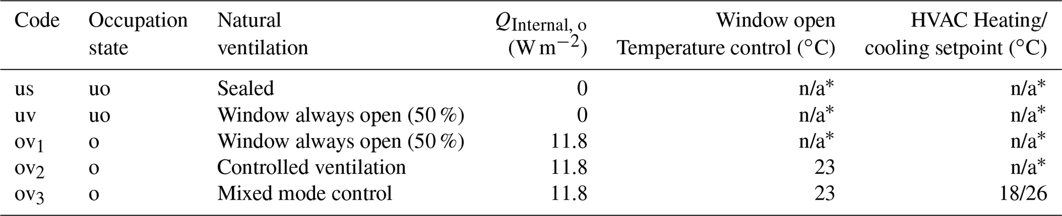
^* n/a stands for not applicable.

The modelling scenarios (Table 1) vary with building occupation state. Two types of unoccupied (uo) buildings are considered. Neither have internal heat gains or HVAC systems, but they differ based on air exchange between (1) unoccupied sealed (us) with no infiltration nor ventilation, and (2) unoccupied ventilated (uv) with 50 % of window area kept open. The single-sided natural ventilation rate is estimated by including both the wind-driven ventilation rate (V_W, m³ s⁻¹) (Warren 1977):

$$\begin{array}{}\text{(16)}& V_{\mathrm{W}}=\mathrm{0.025}{A}_{\text{eff}}{U}_{\mathrm{W}}\end{array}$$

and the stack buoyancy-driven ventilation rate (V, m³ s⁻¹) (Warren 1977):

$$\begin{array}{}\text{(17)}& V_{\text{Stack}}={\displaystyle \frac{\mathrm{1}}{\mathrm{3}}}{A}_{\text{eff}}{C}_{\mathrm{d}}\sqrt{{\displaystyle \frac{\mathrm{\Delta }THg}{T_{\text{ave}}}}},\end{array}$$

where A_eff is the effective opening area (m²), U_W is the reference wind speed at the height of opening (m s⁻¹). C_d is the discharge coefficient (usually taken as 0.6, Wang and Chen (2012)), ΔT is the indoor and outdoor air temperature difference (^∘C), H is the height of opening (m), g the gravitational acceleration (m s⁻²) and T_ave is the average indoor and outdoor air temperature (^∘C). The combined ventilation rate is (Fan et al., 2021)

$$\begin{array}{}\text{(18)}& V_T=\sqrt{V_{\mathrm{W}}^{\mathrm{2}}+V_{\text{Stack}}^{\mathrm{2}}}.\end{array}$$

The three occupied (o) building simulations assume that occupant behaviour modifies internal heat generation, natural ventilation and HVAC systems (ov). First, ov₁ has internal heat gains (Q_{Internal, o}) from human metabolism, lighting and other appliances based on local building code (MOHURD, 2018), with window always open (50 %, as uv). The internal heat gains are held constant allowing the fraction of heat in Q_F,B and ΔQ_S to be impacted by building and climate conditions but not the diurnal variability of human heat generation.

Second, ov₂ considers natural ventilation based on passive cooling and thermal comfort. The window opening is controlled automatically. It is opened (50 % of window area) when the indoor air temperature is higher than both outdoor air temperature and the ventilation setting point (23^∘C for “warm limit” in the bedroom (Oikonomou et al., 2012)). Otherwise, it is closed to reduce heat loss and keep the building warm. Third, since natural ventilation alone may not satisfy indoor thermal comfort, mixed mode ventilation with an auxiliary HVAC system (e.g. Wang and Chen, 2013; Wang and Greenberg, 2015; Chen et al., 2017) is considered in ov₃. The mechanical heating and cooling systems are active when the indoor temperature reaches the threshold (18^∘C for heating and 26^∘C for cooling, MOHURD, 2018). The ventilation control strategy in ov₃ is the same as ov₂, but the EnergyPlus hybrid ventilation manager (DOE, 2020b) turns the HVAC off when natural ventilation is active to prevent simultaneous operation.

2.2 Determination of anthropogenic heat flux

The simulated hourly heat fluxes by radiation, convection, air exchange and waste heat generated from the HVAC system between the isolated building and the atmosphere (Table S3 in the Supplement) are analysed for each case (Table S2 in the Supplement). If cooling occurs, the waste heat consists of the cooling load and electrical energy consumed by the air conditioner (Q_HVAC). The Q_HVAC is predicted using a static coefficient of performance (COP) for the air conditioner, and the heat removed by an air conditioner (Q_AC) to the total amount of electricity consumed:

$$\begin{array}{}\text{(19)}& {\displaystyle }{Q}_{\text{HVAC, C}}={\displaystyle \frac{Q_{\text{AC}}}{\text{COP}}}\text{(20)}& {\displaystyle }{Q}_{\text{Waste,C}}=Q_{\text{AC}}\left(\mathrm{1}+{\text{COP}}^{-\mathrm{1}}\right).\end{array}$$

With a centralised heating system (as Beijing has), for simplicity we assume all energy associated with the heating system is released indoors, and waste heat due to boiler efficiency and pipe heat loss are not considered:

$$\begin{array}{}\text{(21)}& {\displaystyle }{Q}_{\text{HVAC, H}}=Q_{\text{HS}}\text{(22)}& {\displaystyle }{Q}_{\text{Waste, H}}=\mathrm{0}.\end{array}$$

Combining mechanical heating and cooling, the energy consumption and corresponding waste heat from HVAC system gives

$$\begin{array}{}\text{(23)}& {\displaystyle }{Q}_{\text{HVAC}}=Q_{\text{HVAC, C}}+Q_{\text{HVAC, H}}={\displaystyle \frac{Q_{\text{AC}}}{\text{COP}}}+Q_{\text{HS}}\text{(24)}& {\displaystyle }{Q}_{\text{Waste}}=Q_{\text{Waste, C}}+Q_{\text{Waste, H}}=Q_{\text{AC}}\left(\mathrm{1}+{\mathrm{COP}}^{-\mathrm{1}}\right).\end{array}$$

Each term in Eq. (14) is determined using an occupied (o) and unoccupied (uo) building result to determine Q_F,B and the other fluxes. The results are analysed by season as spring (March, April and May, MAM), summer (June, July, August, JJA), autumn (September, October, November, SON) and winter (December, January, February, DJF)) using the median (50 %) and interquartile range (IQR) between the 25th and 75th percentiles to assess the diurnal patterns.

2.3 Ratio of anthropogenic heat flux to energy consumption

If the energy consumed within the building is ejected immediately into the atmosphere (Heiple and Sailor, 2008), the change in ΔQ_S is not accounted for, and therefore Q_F,B is assumed to be only from energy consumption (Q_EC). The variation of ΔQ_S associated with human activities is considered when using the relative heat emissions in Eqs. (14) and (15). We use the ratio $R=\frac{Q_{\mathrm{F},\mathrm{B}}}{Q_{\mathrm{EC}}}$ to determine the relative importance of building operation modes and choice of baselines on the discrepancy between Q_F,B and Q_EC.

3 Results and discussion

Building energy balance fluxes vary through each day and season (Fig. 1) associated with when a building is occupied and people's activities inside the building. First, we consider one case in detail – an occupied building with both natural ventilation and HVAC (ov₃, Table 1) relative to an unoccupied sealed building (us, Table 1) – their difference (ov₃–us) allows us to obtain the fluxes needed (Sect. 1).

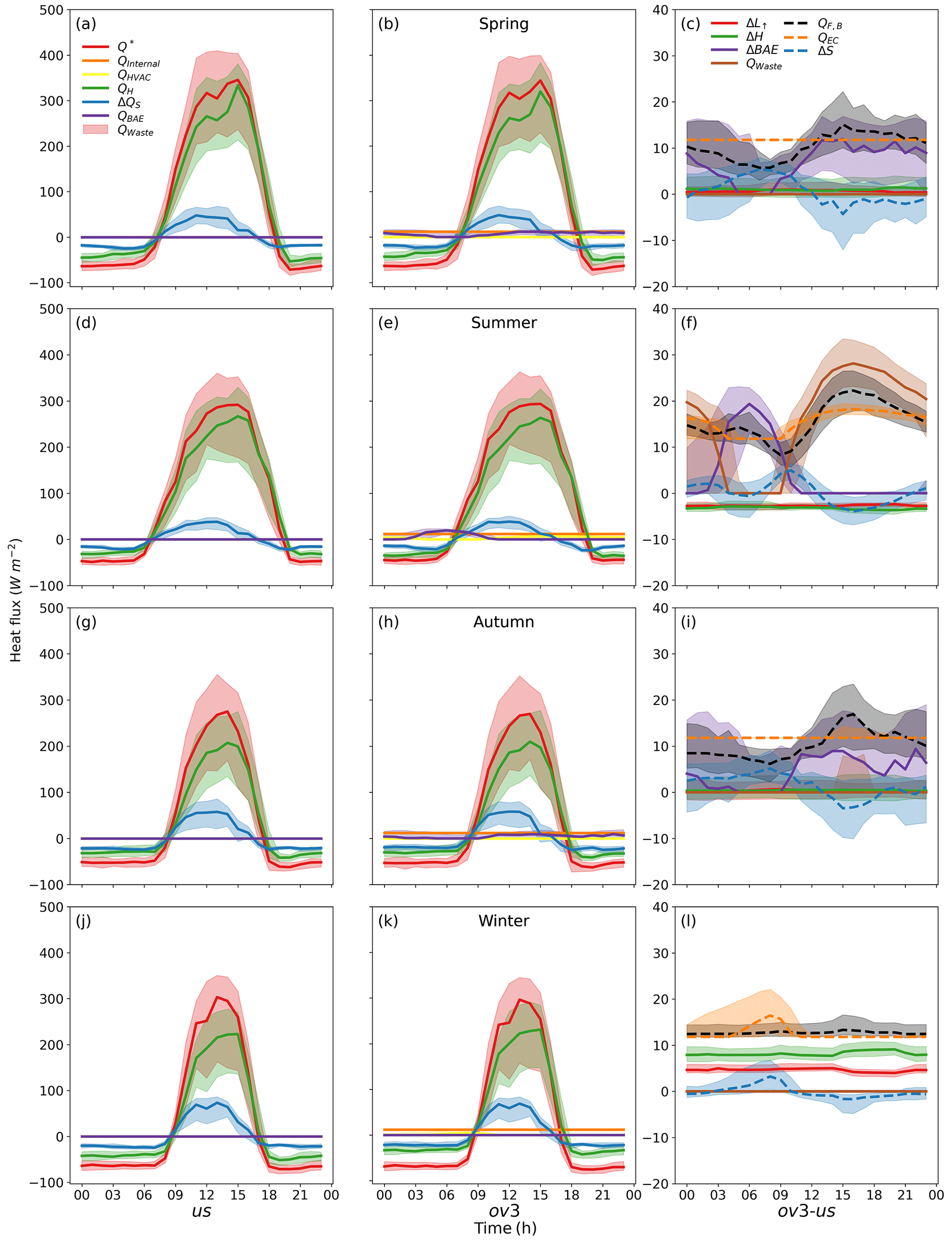
Figure 1 Seasonal diurnal median (line) and interquartile range (IQR, shading) building heat fluxes for (a, d, g, j) unoccupied sealed (us), (b, e, h, k) occupied ventilated (ov₃) building and their (c, f, i, l) difference (ov₃–us) for (a–c) spring, (d–f) summer, (g–i) autumn and (j–l) winter. Q_F,B is estimated by either heat transfer difference (solid line components): $Q_{\mathrm{F},\mathrm{B}}=\mathrm{\Delta }{L}_{\uparrow \text{o-uo}}+\mathrm{\Delta }{H}_{\text{o-uo}}+\mathrm{\Delta }{\text{BAE}}_{\text{o-uo}}+Q_{\text{Waste, o}}$ in Eq. (14) or energy consumption and storage flux difference: $Q_{\mathrm{F},\mathrm{B}}=Q_{\text{EC}}-\mathrm{\Delta }{S}_{\text{o-uo}}$ (dashed line components) in Eq. (15)

As noted (Sect. 1), the shortwave and incoming longwave radiation fluxes for all cases (Table 1) are assumed to be identical, but all other terms of the building energy balance differ. Hence, the change in outgoing longwave radiation (ΔL_↑o-uo, Fig. 1c) is equivalent to the net all-wave radiation difference ($Q_{\text{o-uo}}^{\ast }$, Fig. 1a–b) for the occupied and unoccupied buildings. The positive sensible heat flux difference (Eq. 10, ΔH_o-uo, Fig. 1c) and ΔL_↑o-uo indicate the building is warmed up by internal heat gains (Q_{Internal, o}) with higher exterior surface temperatures. Their small magnitudes and flat patterns indicate small relative importance compared to the heat exchange from ventilation differences (Eq. 8, ΔBAE_o-uo, Fig. 1c). The latter not only contributes the largest fraction of anthropogenic heat flux ($Q_{\mathrm{F},\mathrm{B}},$ Fig. 1c), but also has a diurnal pattern consistent with Q_F,B, especially during spring and autumn (Fig. 1c, i). Rarely, heat (Q_{Waste, o}, Fig. 1i) is emitted by the air conditioner in the mid-afternoon (shading) at this time of year, but more importantly in summer (Fig. 1f) when cooling demand increases.

The Q_F,B (Eq. 14, Fig. 1c) has four components of emitted heat, whereas energy consumption (Q_EC, Fig. 1c) only has (in this case, constant) internal heat gains (Q_{Internal, o}=11.8 W m⁻², Fig. 1b, Table 1) and energy use from HVAC systems (Q_HVAC, Fig. 1b). Their difference is the storage heat flux difference (Eq. 15 ΔS_o-uo in Fig. 1c). If ΔS_o-uo is positive, the building acts as a heat sink and stores the extra heat generated by human activities, or stored heat is released when ΔS_o-uo is negative. Hence, we can identify the impacts of seasonal varying human activities and building operations on the diurnal variability in ΔS_o-uo, Q_EC and Q_F,B.

3.1 Impact of human activities on seasonal and diurnal variations of the fluxes

For the same ov₃–us case (Table 1, Fig. 1), we consider the diurnal and seasonal variability of the fluxes. In spring and autumn (Fig. 1a–c, g–i), natural ventilation is the dominant factor contributing to diurnal variation in ΔS_o-uo and Q_F,B, while Q_EC has minimal variability. The Q_EC is slightly larger than Q_{Internal, o} because of some short periods of HVAC use in the mid-afternoon (IQR shading in Fig. 1i). There is a clear diurnal cycle of Q_F,B (Fig. 1c) with the median varying between 8 W m⁻² (07:00) and 15 W m⁻² (15:00) relative to the constant internal heat gain (11.8 W m⁻²). The difference between Q_F,B and Q_EC (ΔS_o-uo) is largely impacted by natural ventilation. During the night and early morning with closed windows, only part of the consumed energy is transferred externally to the atmosphere. The rest of the heat is stored in the building fabric (positive ΔS_o-uo), hence Q_F,B is lower than Q_EC. However, when overheating may occur during the middle of the day, occupants keep the window opened (air conditioner is less frequently used) to cool the building down, with stored heat released (negative ΔS_o-uo). This is consistent with the diurnal variability of ΔBAE_o-uo, which has a minimum at night (window closed) and maximum in the mid-afternoon (window open).

In summer, the daytime natural ventilation is replaced by air conditioning as natural ventilation alone could not maintain thermal comfort indoors. Natural ventilation and waste heat from the air conditioner (Q_{Waste, o}) contribute to one peak Q_F,B at nighttime and daytime, respectively (Fig. 1f). Q_F,B is higher than Q_EC around these two peak periods (05:00–07:00 and 13:00–21:00). The peak Q_F,B at night reaches 14 W m⁻² (median) at 05:00, which is mainly attributed to natural ventilation when outdoor air temperature is cooler than indoors. Conversely, in the afternoon when outdoor temperature is warmer, occupants “choose” mechanical cooling to achieve thermal comfort. The peak Q_F,B is 22 W m⁻² at 16:00, approximately 22 % higher than Q_EC. It indicates that using Q_EC for the anthropogenic heat flux from buildings (e.g. Heiple and Sailor, 2008) may underestimate the effect of Q_F,B on urban atmospheric processes especially during the late afternoon/early evening. In addition, Q_F,B is always smaller than Q_{Waste, o} because of the negative ΔL_↑o-uo and ΔH_o-uo causing a cooler exterior surface. This suggests using Q_{Waste, o} as Q_F,B (e.g. Chow et al., 2014) may overestimate Q_F,B in summer.

However, in winter mechanical heating and thermal mass effect shape the temporal pattern of Q_F,B (Fig. 1i). The cool outdoor air temperature before sunrise results in a substantial heating supply and peak Q_EC (16.43 W m⁻² for median line) at 08:00. This heat is stored in building fabric (positive ΔS_o-uo) and has a relatively stable release through convection and longwave radiation. Therefore the diurnal profile Q_F,B is rather flatter and ΔS_o-uo has a highly consistent temporal pattern to Q_EC.

Overall, this analysis recognises the crucial role of ΔS_o-uoin distinguishing Q_F,B from Q_EC, which is highly dependent on HVAC operation and natural ventilation (i.e. human activity of window opening). These two factors can rapidly increase or decrease Q_F,B while convection and longwave radiation cannot. Whereas in winter, the larger IQR (shading) of Q_F,B than Q_EC indicates more day-to-day variation in Q_F,B diurnal profile than Q_EC. Estimates of Q_F,B using satellite remote sensing found heat storage plays an important role in moderating energy use within buildings (Yu et al., 2021). As the storage heat flux change modifies the diurnal sensible heat flux pattern it modifies the surface temperature increment (Q_F,B in remote sensing approach) and hence the apparent energy consumption.

The diurnal profiles of ΔS_o-uo are not identical between seasons as people use different actions to achieve thermal comfort in different weather conditions. This suggests that the Q_F,B and Q_EC differences may vary between climates and with cultural practices. In inventory methods the diurnal profiles may be limited, e.g. large scale urban consumption of energy (LUCY, Allen et al. (2011), weekday/weekend by country, and ignore seasonal variations. However, ΔS_o-uo behaviour type classes may benefit from distinguishing diurnal variation for different climates.

3.2 Impact of different building operation modes on seasonal and diurnal variations

Figure 2 illustrates the impact of different building operation modes (Table 1: ov₁, ov₂, ov₃; cf. us) on the Q_F,B diurnal profiles. It suggests that the different ventilation strategies and HVAC systems do change Q_F,B in both temporal pattern and magnitude, but their impacts vary among seasons.

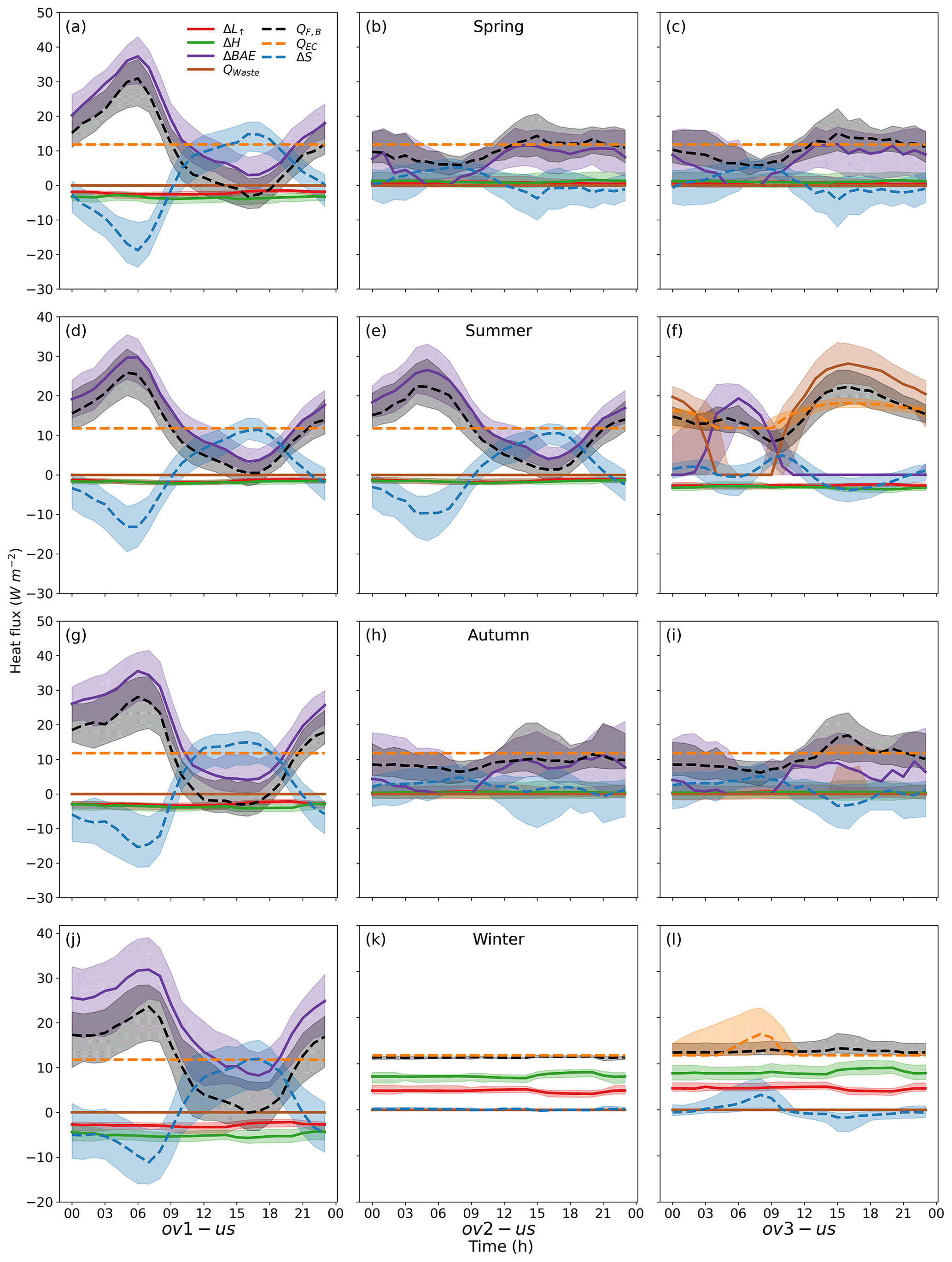
Figure 2 As Fig. 1c, f, i, j , but comparing three different building operation types (a, d, g, j) ov₁: window is always open without control, no HVAC; (b, e, h, k) ov₂: controlled natural ventilation for indoor thermal comfort, no HVAC; (c, f, i, l) ov₃: mixed mode ventilation.

In spring and autumn, different natural ventilation control strategies completely modify the Q_F,B diurnal profile, whereas a HVAC system only increases the peak Q_F,B slightly in autumn (Fig. 2i). The distinctly different (opposite) trend in diurnal Q_F,B pattern for ov₁ cf. ov₂ or ov₃ (Fig. 2a–c, g–i) is largely explained by the diurnal change of ΔBAE_o-uo in the three cases. In ov₁ (window open, no control) the minimum outdoor air temperature before sunrise creates the maximum indoor and outdoor air temperature difference, therefore the highest ΔBAE_o-uo and peak Q_F,B at 06:00 (30 W m⁻² for the median in Fig. 2a). Whereas ov₂ and ov₃ have the window closed at night and early morning to avoid overcooling, therefore, the minimum Q_F,B is in the early morning (07:00). As outdoor air temperature increases through the day, Q_F,B follows the reduced ΔBAE_o-uo in ov₁, whereas natural ventilation is active in ov₂ and ov₃, leading to an increase in ΔBAE_o-uo and Q_F,B. Unlike ov₂, ov₃ has a clear peak (16 W m⁻² median, Fig. 2i) at 15:00, because natural ventilation alone cannot satisfy thermal comfort and ov₃ air conditioning is activated. But their overall patterns (IQR) are very consistent, indicating afternoon use of air conditioning could increase Q_F,B magnitude but have a limited impact on other parts of the diurnal pattern. Surprisingly, negative Q_F,B occurs around 17:00 in spring (Fig. 2a), suggesting the occupied building has less heat emission than the unoccupied building, because the natural ventilation at night and morning cools the building down and reduced fabric exterior surface temperature leads to a larger reduction in longwave radiation and convection (ΔL_↑o-uo and ΔH_o-uo) than the increase in heat emission through natural ventilation (ΔBAE_o-uo) in the afternoon. Also, the reduced overall emissions are converted into increase in storage heat flux (ΔS_o-uo). Negative Q_F,B also occurs when the unoccupied building is always ventilated (uv) and the occupied building is ventilated with control (ov₂ and ov₃) in spring (e.g. Fig. S7b–c in the Supplement). The window is closed to avoid excessive cooling at night in ov₂. With ΔBAE_o-uo negative in this case, its magnitude is much larger than the increase in longwave radiation and convection ($\mathrm{\Delta }{L}_{\uparrow \mathrm{o}-\mathrm{uo}}$ and ΔH_o-uo). The minimum Q_F,B frequently corresponds to the peak ΔS_o-uo.

In summer, in ov₂ the window is open most of the time (as in ov₁) for thermal comfort, therefore, the Q_F,B has no apparent difference to ov₁. However for ov₃, as the air conditioning runs from morning to late night there is a very different diurnal profile (cf. ov₂ and ov₁). Air conditioner use contributes to a much larger Q_F,B (cf. ov₂) from 12:00 to 21:00. Not only is extra energy consumed, but it also removes heat from the building to the atmosphere in this period. In contrast, using natural ventilation as a cooling strategy (ov₁ and ov₂) contributes to a high Q_F,B at night and early morning but very low even negative extra heat emission in the afternoon. This implies that natural ventilation as a passive cooling strategy could not only improve the thermal conditions indoors but could also contribute to the improvement of outdoor climate by modifying the diurnal pattern of anthropogenic heat emissions (Duan et al., 2019).

Consistent with results in the other seasons, different ventilation control strategies in winter cause a large change in the Q_F,B profile between ov₁ and ov₂. However, the temporal pattern of Q_F,B (IQR) in ov₂ is quite similar to ov₃ because the supplied heat from the mechanical heating system does not immediately enhance Q_F,B with a closed window. Ov₂ is the only scenario that has similar Q_F,B and Q_EC through the whole day. Comparison using an unoccupied ventilated (uv) baseline (Fig. S7) (cf. us Fig. 2) show that although Q_F,B profiles differ, the impacts of different building operation modes are consistent when the same occupied buildings are used. The impact of baselines with different air exchange on Q_F,B are analysed in Sect. 3.3.

3.3 Impact of unoccupied baseline chosen

Here two unoccupied baselines (us – unoccupied sealed building, uv – unoccupied ventilated building with uncontrolled open window) are used to assess the impact. A ratio between Q_F,B and Q_EC (R) is used (Fig. 3) to normalise the impact of baselines on their difference with different building operation modes. The largest difference in R occurs on 23 December at 11:00, with values of 5.13 (ov₃–uv) and −2.72 (ov₁–us), reflecting the considerable difference between Q_F,B and Q_EC.

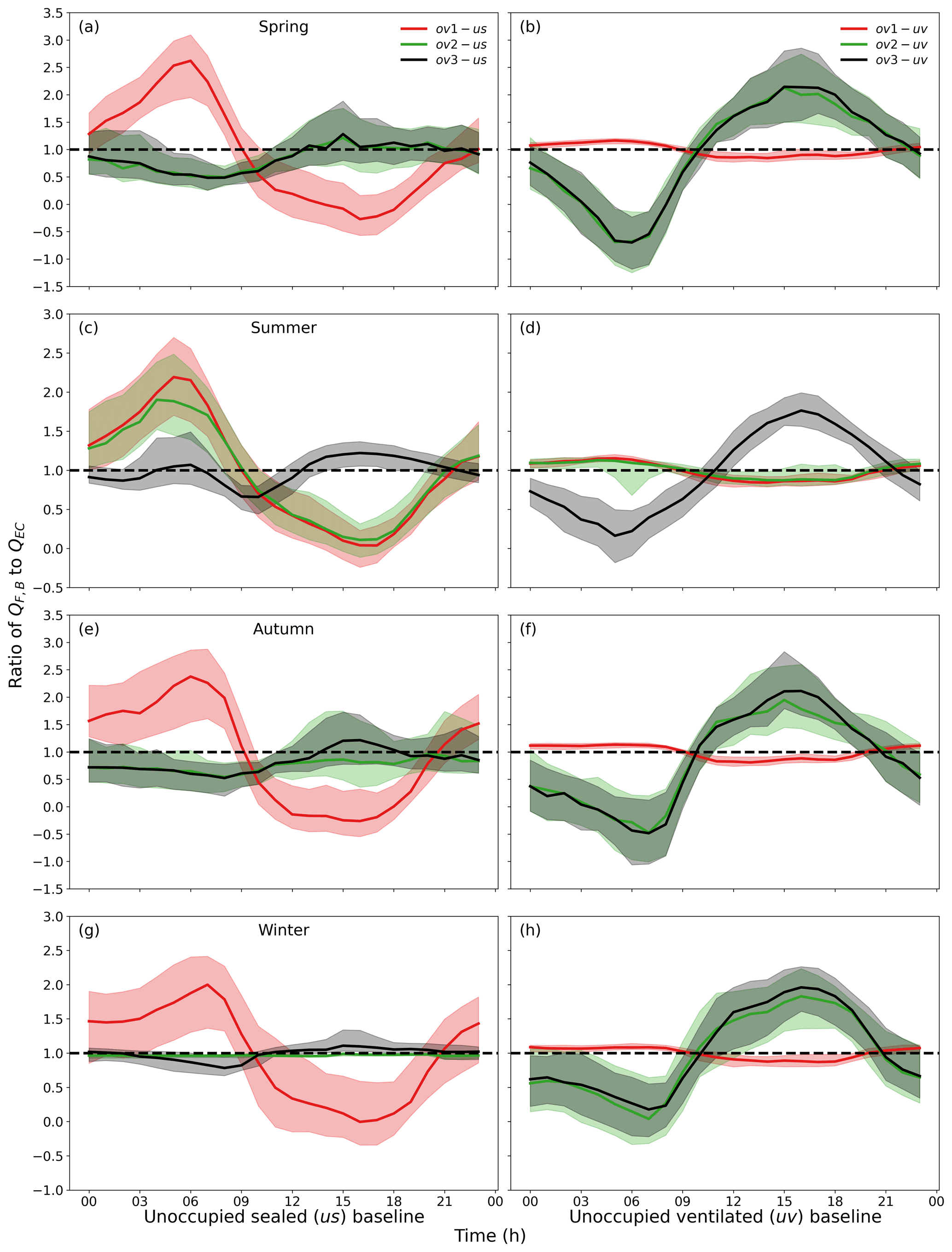
Figure 3 Q_F,B to Q_EC ratio I median (line) and IQR (shading) for (a–b) spring, (c–d) summer, (e–f) autumn and (g–h) winter, using two unoccupied baselines: (a, c , e, g) sealed (us), and (b, d, f, h) ventilation (uv); each with three occupancy types (colour): ov₁: only internal heat gains are applied and window is fully open; ov₂: internal heat gains and natural ventilation control are applied. Ov3: internal heat gains, natural ventilation control and HVAC system are applied. Ratio R=1 (Black dotted line).

Two diurnal patterns of the R ratio are distinguished. When the window is always open (ov₁ in all seasons, ov₂ in summer), R>1 (Q_F,B>Q_EC) at night/early morning (22:00–08:00), reaching its maximum around 05:00–07:00 (near sunrise in all seasons). For the remaining periods, which are relatively warm R<1. Whereas, when window opening/closing is controlled and HVAC is used for thermal comfort an almost inverse temporal pattern of R occurs, with R>1 during the afternoon when either the window is open or the air conditioner is activated. The peak R occurs at 15:00 when both outdoor temperature and solar radiation are high.

When different unoccupied baselines are used, the temporal patterns of R are similar for all cases, but their magnitudes differ significantly. R is close to 1 when window states between unoccupied and occupied buildings are similar (e.g. ov₁–uv in all seasons, ov₂–uv in summer). Hence, a greater difference occurs in heat transfer from ventilation or mechanical heating/cooling between occupied and unoccupied buildings (i.e. larger R). Thus, the baseline chosen impacts the results and requires appropriate consideration for incorporating Q_F,B into atmospheric modelling.

3.4 Comparison between Q_F,B and building heat emission (BHE)

Comparison of building heat emissions (BHE), determined using the Hong et al. (2020) approach, to Q_F,B (this study) for one case (ov₃–us) shows that the former is much larger than Q_F,B during the day but smaller at night and has different diurnal patterns (Fig. 4). Convection from the exterior envelope (Q_H, Fig. 1b, e, h, k) is the main contributor to BHE and therefore influences the BHE diurnal profile in each season. During the day, solar radiation is high and a major control whereas Q_F,B is relatively small and consistent but modified by building-human interactions (e.g. opening windows, activation of mechanical heating and cooling systems). In this scenario shown, natural ventilation and mechanical cooling dominate Q_F,B in summer and shoulder season (i.e. spring and autumn); while in winter in their absence, convection and longwave radiation are more important.

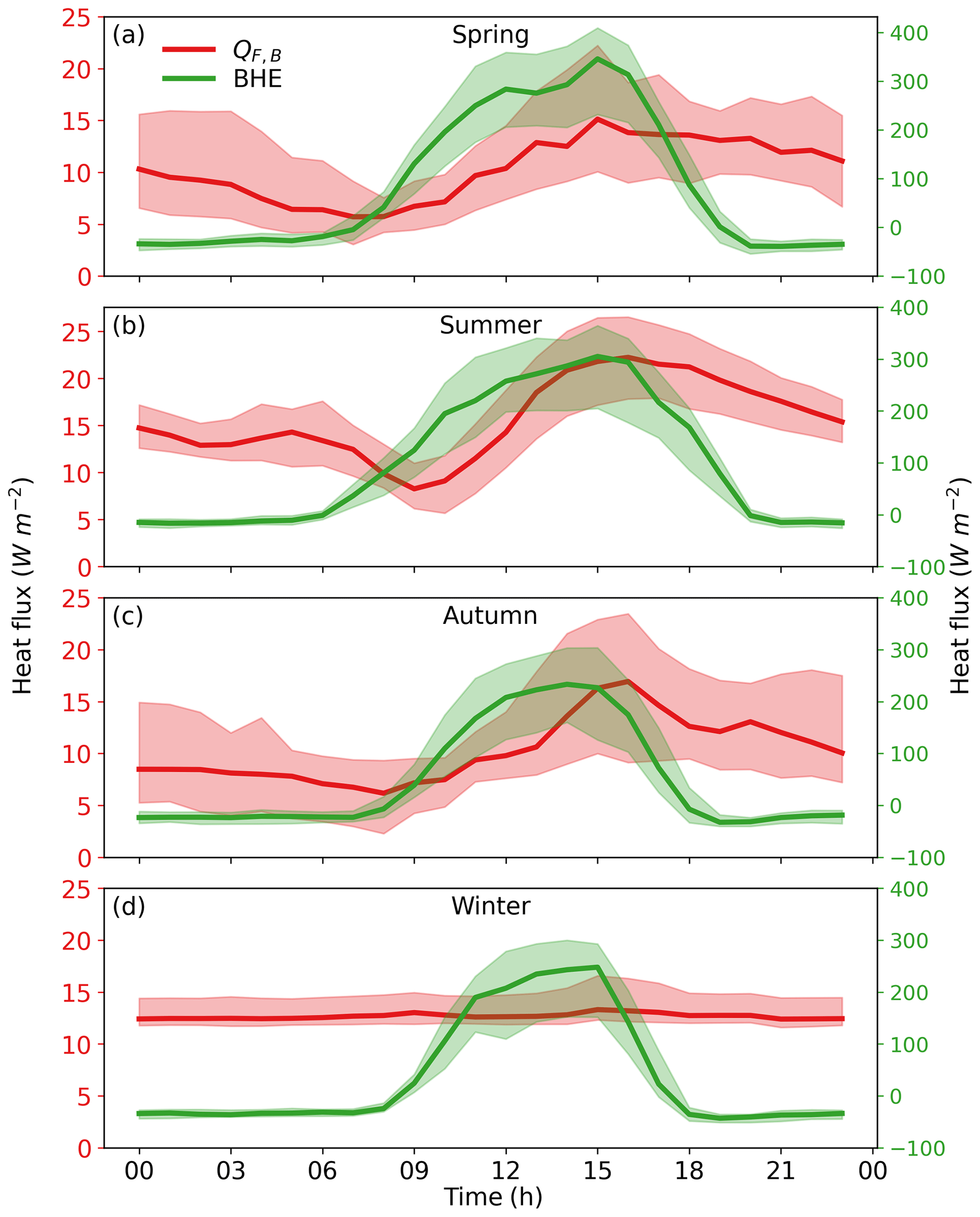
Figure 4 Comparison of seasonal diurnal Q_F,B (ov₃–us) and building heat emission (BHE, ov₃ in Table 1) for (a) spring, (b) summer, (c) autumn and (d) winter.

3.5 Daily variation of fluxes in relation to meteorological conditions

Ambient air temperature is one of the most crucial factors controlling building energy consumption (Sailor and Vasireddy, 2006). Hence, it is often used to determine daily variability of Q_EC (e.g. Lindberg et al., 2013) and the resulting monthly variations (e.g. Allen et al., 2011). By accounting for ΔS_o-uo in this study, the response of Q_F,B to ambient air temperature may differ to previous studies. To examine this we used the ov₃–us case to consider the relations of daily mean (unless indicated) variables of air temperature (mean) , solar radiation (daily total) and simulated available energy to the building from human activities (ΔB_o-uo) with anthropogenic heat flux (Q_F,B in Fig. 5a), energy consumption (Q_EC in Fig. 5b) and their difference (ΔS_o-uo in Fig. 5c).The overall trends between Q_F,B and Q_EC to ambient air temperature are consistent, with Q_F,B and Q_EC smallest when temperatures are between 10–15 ^∘C. This coincides with the Nicol and Humphreys (2002) monthly balance-point temperature of 12 ^∘C, which has been regarded as the equivalent ambient air temperature with the minimum energy use within the building (e.g. Allen et al., 2011, Koralegedara et al., 2016). As the temperature increases (decreases), Q_EC increases proportionally with temperature due to mechanical cooling (heating). However, in contrast to Q_EC, Q_F,B has a much larger variability at the same temperature caused by a large range of ΔS_o-uo (−7.7 to 9.0 W m⁻²), which is highly dependent on human activities on the diurnal scale (Sect. 3.1).

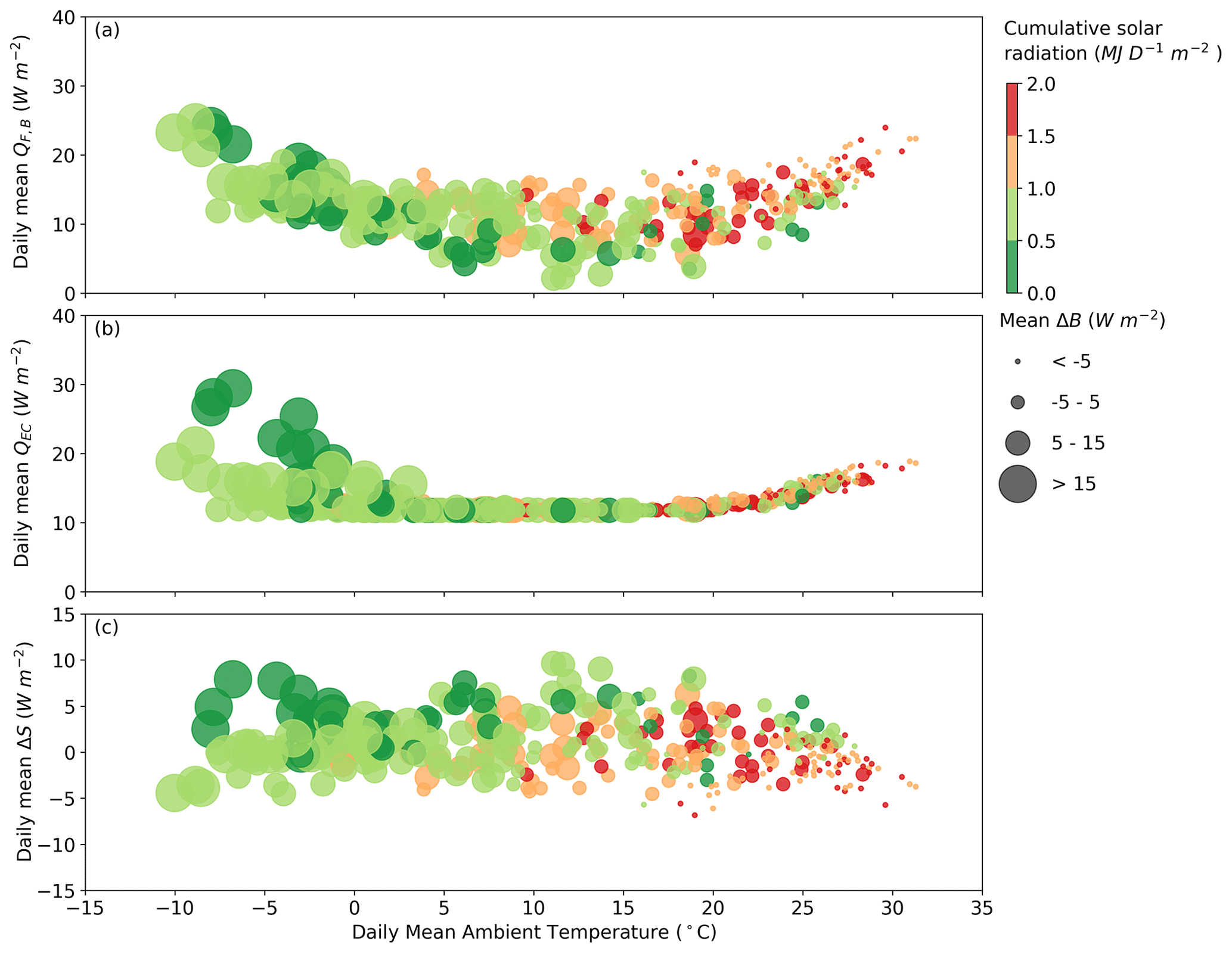
Figure 5 Daily results for the ov₃–us case stratified by daily cumulative solar radiation (colour) and daily mean available energy to the building (size) Eq. (9) associated with human activities, with mean external air (ambient) temperature and (a) mean anthropogenic heat flux, (b) energy consumption and (c) difference in storage heat flux.

To understand the large daily variability of ΔS_o-uo, we use ΔB_o-uo (net available energy from human activities in buildings in Eq. (9)) to indicate the effect of human activities (heat addition or removal) in one day. Higher ΔB_o-uo (larger circles) are associated with higher ΔS_o-uo at the same ambient air temperature, especially in winter (Fig. 5c). This is not unexpected as buildings will absorb more heat when extra internal energy is added into the building. Inversely, negative ΔB_o-uo (small circles) contributes to much more heat release from heat storage (lower ΔS_o-uo through either natural ventilation or mechanical cooling. The sign and magnitude of ΔB_o-uo are linked to daily cumulative solar radiation. At the same ambient air temperature, more solar radiation enhances the need for larger heat removal or less heat addition to the building for thermal comfort, therefore leading to a smaller ΔB_o-uo and lower ΔS_o-uo. Consequently, we can conclude that both ambient air temperature and cumulative solar radiation are important meteorological factors to determine ΔS_o-uo and Q_F,B.

4 Conclusions

Anthropogenic heat flux from buildings (Q_F,B) is defined as the additional heat released from the building into the atmosphere due to human activities. It is qualitatively and quantitatively different to building energy consumption (Q_EC) in temporal pattern and magnitude as a result of thermal inertia of the building (Iamarino et al., 2012). However, as there is no standard to quantify “real” Q_F,B most studies use Q_EC as a proxy via inventory and building energy modelling approaches. This paper proposes a new method to quantify a more appropriate Q_F,B by utilising the difference in heat fluxes between an occupied and unoccupied building (i.e. the built structure with absolutely no energy use and no human metabolism). We show that the difference between Q_EC and Q_F,B is attributable to a change in the storage heat flux induced by human activities (ΔS_o-uo). Q_F,B has four components based on its dissipation pathways, including outgoing longwave radiation, turbulent sensible heat flux (convection), heat release due to air exchange and waste heat from HVAC systems. We use one simplified case study in Beijing to demonstrate the analysis using building energy simulations to quantify the temporal difference between Q_EC and Q_F,B and to understand the relative importance of building operations for thermal comfort and meteorological conditions on Q_F,B. The key conclusions are

1. Hourly ratios between Q_F,B and Q_EC can differ between −2.72 and 5.13 because of differences in occupancy use of the building (within a year, in Beijing's climate). Individual ratios frequently exceed 3 between 14:00 and 16:00 when controlled natural ventilation or mechanical cooling is activated in a shoulder season (i.e. spring and autumn). Thus, the differences in the definitions are large.

2. Natural ventilation (ΔBAE_o-uo) or HVAC operation (Q_{Waste, o} for cooling and Q_HVAC for heating) are two predominant contributors to the storage heat flux. Hence, different building operations to control thermal comfort determine the diurnal profile of Q_F,B by affecting not only Q_EC but also ΔS_o-uo.

3. The day-to-day variation of the Q_F,B diurnal profile is broader than that of Q_EC.

4. The diurnal profile of ΔS_o-uo varies with season as occupants modify their behaviour and the interaction with buildings to achieve thermal comfort (e.g. cooling in summer and heating in winter), indicating that differences between Q_F,B and Q_EC will vary with both climate and cultural norms.

5. Q_F,B is sensitive to the unoccupied baseline chosen (here two are analysed unoccupied sealed vs unoccupied ventilated). An “unoccupied baseline” needs to be integrated into urban climate modelling in the future.

6. Daily mean temperature only accounts for the day-to-day variability in Q_EC rather than ΔS_o-uo. Both ambient air temperature and cumulative solar radiation are important meteorological factors to determine ΔS_o-uo and Q_F,B.

Our new approach should be used to provide data for future parameterisations of both anthropogenic heat flux from buildings and storage heat fluxes for urban weather and climate modelling. We conclude that storage heat fluxes in cities are also being modified by occupant behaviour, particularly by natural ventilation and mechanical cooling. It is expected that the diurnal variation of ΔS_o-uo will vary with operation schedules for different building uses (e.g. residential vs. commercial buildings). Given that the release of stored heat has a critical influence on the nocturnal canopy layer urban heat island (CL-UHI), the impact of different HVAC operations on nocturnal UHI should be explored further. This is an important factor to determine diurnal pattern of Q_F,B in the shoulder season and can be expressed more accurately. However, in different climates and with different social cultural practices the periods most influenced will change. Further studies are being conducted to explore the impacts of these, while also addressing feedback at the neighbourhood scale.

For developers of urban canopy parameterisations (UCP) there are several considerations because of computational efficiencies which are essential for undertaking weather and climate modelling: (1) human activities within a building are modifying both the storage heat flux and the anthropogenic heat flux; (2) assuming within an UCP that a “simple” building energy model (BEM) (cf. a full building energy simulation scheme such as EnergyPlus) will require some human activities to be simplified, such as using a fixed ventilation rate, instead of dynamic natural ventilation depending on both outdoor weather conditions and thermal comfort requirements and (3) with a multi-layer UCP the appropriate levels for the impact of these energy exchanges can be accounted for. Our current research is extending this analysis to consider moisture and exploring the role of building materials, construction, other aspects of building design and external meteorology. The outcome of this work will also have implications for UCP development, as this can help identify what can be simplified and what are critical controls in different climates and urban settings.

Appendix A: Nomenclature

Aeff	Effective area of window opening (m2)
ΔBo-uo	Available energy to the building from human activities (W m−2)
Δ BAEo-uo	Difference of heat transfer by air exchange between building and atmosphere between occupied (o)
	and unoccupied (uo) buildings (W m−2)
BHE	Building heat emission to ambient air (W m−2)
ΔHo-uo	Difference in QH between occupied (o) and unoccupied (uo) buildings (W m−2)
F[sky→boi]	View factor from sky to building of interest
F[other b→boi]	View factor from other buildings to building of interest
F[boi→sky]	View factor from building of interest to sky
F[boi→other b]	View factor from building of interest to other buildings
Cd	Discharge coefficient
H	Height of window opening (m)
K↑	Outgoing shortwave radiation flux (W m−2)
K↓	Incoming shortwave radiation flux (W m−2)
L↑	Outgoing longwave radiation flux (W m−2)
L↓	Incoming longwave radiation flux (W m−2)
ΔL↑o-uo	Difference in L↑ between occupied (o) and unoccupied (uo) buildings (W m−2)
ΔQS	Net storage heat flux for the building volume (W m−2)
Q∗	Net all-wave radiation flux (W m−2)
QAC	Sensible cooling load from air conditioning (W m−2)
QBAE	Heat transfer by air exchange between building and atmosphere (W m−2)
QF,B	Anthropogenic heat flux from building sector (W m−2)
QF,M	Anthropogenic heat flux from metabolic activities (W m−2)
QF,T	Anthropogenic heat flux from transport (W m−2)
QH	Turbulent sensible heat flux (W m−2)
QHS	Sensible heating load (W m−2)
QHVAC	Energy consumption by heating ventilation and air conditioning (HVAC) system (W m−2)
QInternal	Internal heat gain within the building (human metabolism, lighting and appliances) (W m−2)
QWaste	Waste heat released to outdoor by HVAC system (W m−2)
R	Ratio of anthropogenic heat flux from building (QF,B) to energy consumption (QEC)
ΔSo-uo	Different in storage heat flux between occupied (o) and unoccupied (uo) buildings (W m−2)
Tave	Average indoor and outdoor air temperatures (∘C)
ΔT	Indoor and outdoor air temperature difference (∘C)
UW	Reference wind speed at height of upstream airflow (m s−1)
VStack	Buoyancy-driven ventilation rate (m3 s−1)
VT	Total ventilation rate by combined wind and buoyancy effect
VW	Wind-driven ventilation rate (m3 s−1)