Environmental effects on aerosol–cloud interaction in non-precipitating marine boundary layer (MBL) clouds over the eastern North Atlantic

Over the eastern North Atlantic (ENA) ocean, a total of 20 non-precipitating single-layer marine boundary layer (MBL) stratus and stratocumulus cloud cases are selected to investigate the impacts of the environmental variables on the aerosol–cloud interaction (ACI_r) using the ground-based measurements from the Department of Energy Atmospheric Radiation Measurement (ARM) facility at the ENA site during 2016–2018. The ACI_r represents the relative change in cloud droplet effective radius r_e with respect to the relative change in cloud condensation nuclei (CCN) number concentration at 0.2 % supersaturation (N_CCN,0.2 %) in the stratified water vapor environment. The ACI_r values vary from −0.01 to 0.22 with increasing sub-cloud boundary layer precipitable water vapor (PWV_BL) conditions, indicating that r_e is more sensitive to the CCN loading under sufficient water vapor supply, owing to the combined effect of enhanced condensational growth and coalescence processes associated with higher N_c and PWV_BL. The principal component analysis shows that the most pronounced pattern during the selected cases is the co-variations in the MBL conditions characterized by the vertical component of turbulence kinetic energy (TKE_w), the decoupling index (D_i), and PWV_BL. The environmental effects on ACI_r emerge after the data are stratified into different TKE_w regimes. The ACI_r values, under both lower and higher PWV_BL conditions, more than double from the low-TKE_w to high-TKE_w regime. This can be explained by the fact that stronger boundary layer turbulence maintains a well-mixed MBL, strengthening the connection between cloud microphysical properties and the below-cloud CCN and moisture sources. With sufficient water vapor and low CCN loading, the active coalescence process broadens the cloud droplet size spectra and consequently results in an enlargement of r_e. The enhanced activation of CCN and the cloud droplet condensational growth induced by the higher below-cloud CCN loading can effectively decrease r_e, which jointly presents as the increased ACI_r. This study examines the importance of environmental effects on the ACI_r assessments and provides observational constraints to future model evaluations of aerosol–cloud interactions.

1 Introduction

Clouds are one of the most important parts of the Earth's climate system. They can impact the global climate by modulating the radiative balance in the atmosphere. Moreover, the radiative effects of cloud adjustments due to aerosols remain one of the largest uncertainties in climate modeling (IPCC, 2013). Over the oceanic area, the lower troposphere is dominated by marine boundary layer (MBL) clouds. MBL clouds can persistently reflect the solar radiation by their long-lasting nature maintained by cloud-top radiative cooling and therefore act as a major modulator of the Earth's radiative budget (Seinfeld et al., 2016). The climatic importance of MBL cloud radiative properties is primarily induced by cloud microphysical properties such as cloud droplet number concentration (N_c) and effective radius (r_e) and has been intensively investigated by many researchers (Garrett and Zhao, 2006; Rosenfeld, 2007; Wood et al., 2015; Seinfeld et al., 2016). The ambient aerosol conditions can influence these cloud microphysical properties via the aerosol–cloud interaction (ACI). Compared to the clean regions, clouds under the regions having higher below-cloud aerosol concentrations exhibited smaller cloud droplets (reduced r_e and increased N_c) and enhanced both cloud liquid water contents and optical depths (McComiskey et al., 2009; Chen et al., 2014; Wang et al., 2018). The changes in MBL cloud microphysical properties induced by aerosols have been investigated in previous studies using in situ measurements, ground- and satellite-based observations, and model simulations in multiple oceanic areas such as the eastern Pacific and eastern Atlantic (Twohy et al., 2005; Lu et al., 2007; Hill et al., 2009; Costantino and Bréon, 2010; Mann et al., 2014; Dong et al., 2015; Diamond et al., 2018; Yang et al., 2019; Zhao et al., 2019; Wang et al., 2020).

The assessments of ACI, particularly using ground-based remote sensing, vary in terms of their quantitative values, which represent the different cloud susceptibilities to aerosol loadings. Owing to the numerous approaches in assessing the ACI, such as the spatial and temporal scales; N_c and r_e retrieval methods; and, more importantly, the different aerosol proxies used in the ACI quantification, different ACI results could be achieved. For example, the studies using total aerosol number concentration and aerosol scattering/extinction coefficients to represent the aerosol loadings would result in lower ACI values (Pandithurai et al., 2009; Liu et al., 2016). This is primarily attributed to the inclusion of aerosol species with different abilities to activate, which is determined by their physicochemical properties, and thus will cause non-negligible uncertainties in capturing the information of aerosol intrusion into the cloud (Feingold et al., 2006; Logan et al., 2014), while some studies found higher ACI values using cloud condensation nuclei (CCN) number concentration (N_CCN), presumably due to the fact that CCN represent the portion of aerosols that can be activated and possesses the potential ability to further grow into cloud droplets, thus favorably yielding a more straightforward assessment of ACI (McComiskey et al., 2009; Qiu et al., 2017; X. Zheng et al., 2020). It is noteworthy that the ACI variations have been found to have both increasing and decreasing trends in response to changing environmental water availability (Martin et al., 1994; Martins et al., 2011; Kim et al., 2008; McComiskey et al., 2009; Pandithurai et al., 2009; Liu et al., 2016; X. Zheng et al., 2020). Although these contradicting results have been postulated due to multiple factors such as cloud adiabaticity, condensational growth, collision coalescence, and atmospheric thermodynamics and dynamics, the underlying mechanisms in altering the ACI and causing the uncertainties in the ACI assessments remain unclear. Therefore, further studies are necessary (Fan et al., 2016; Feingold and McComiskey, 2016; Seinfeld et al., 2016).

The eastern North Atlantic (ENA) is a remote oceanic region that features persistent but diverse subtropical MBL clouds, owing to complex meteorological influences from the semi-permanent Azores High and prevailing large-scale subsidence (Wood et al., 2015). The ENA has become a favorable region for studying the aerosol indirect effects on MBL clouds under a relatively clean environment with occasional intrusions of long-range transport of continental air mass (Logan et al., 2014; Wang et al., 2020). The Atmospheric Radiation Measurement (ARM) Program established the ENA permanent observatory site on the northern edge of Graciosa Island, the Azores, in 2013, which continuously provides comprehensive measurements of the atmosphere, radiation, cloud, and aerosol from ground-based observation instruments. Owing to the location of the site, which sits in between the boundaries of mid-latitude and subtropical regimes, the ENA is under the mixed influence of diverse meteorological conditions. In terms of the aerosol influence on the cloud properties, the roles of meteorological factors in cloud formation and development are not negligible and hence are being explored in this study. The large-scale thermodynamic variables of the lower troposphere are widely used, such as the lower tropospheric stability (LTS), where the higher LTS values are found to be associated with a relatively shallow and well-mixed marine boundary layer and are prone to stratiform cloud formations with higher cloud fractions (Klein and Hartmann, 1993; Wood, 2012; Wood and Bretherton, 2006; Yue et al., 2011; Rosenfeld et al., 2019), especially over the subtropical ocean such as the northeast Atlantic. Over the ENA site, the spatial gradient of the LTS has been studied and associated with the contribution terms of MBL turbulence and the wind directional change (Wu et al., 2017).

In the cloud-topped MBL, which is maintained by cloud-top radiative cooling, the buoyancy generation and shear contribute most to the turbulence kinetic energy (TKE) production (Nicholls, 1984; Hogan et al., 2009), where the intensity of turbulence denotes the coupling of MBL clouds to the below-cloud boundary layer. In terms of the cloud droplet growth process, especially in a clean environment with low N_CCN below the cloud layer, the cloud droplets at the cloud base experience rapid growth via the diffusion of water vapor and subsequently enter the regime of active coalescence (Rosenfeld and Woodley, 2003; Martins et al., 2011). The intensive turbulence effectively modulates the cloud droplet growth by strengthening the coalescence process and the cloud cycling (Feingold et al., 1996, 1999; Pawlowska et al., 2006). In particular, the unique topography of Graciosa Island induces an island effect which could cause disturbances in the updraft and hence impact the MBL turbulence, depending on the surface wind directions (Zheng et al., 2016). The environmental effects on the MBL cloud formation and development processes and cloud microphysical properties have been widely implemented and considered in climate modeling (Medeiros and Stevens, 2011; West et al., 2014; Zhang et al., 2016). Thus, it is important to provide observational constraints on the environmental effects. The assessment of ACI from the ground-based perspective highly relies on the sensitivities of cloud droplet number concentrations and size distribution to the changing of below-cloud CCN loadings. Hence, studying the relationship between the environmental effect and the MBL cloud microphysical responses is a nontrivial task.

In this study, we target the non-precipitating single-layer MBL stratus and stratocumulus clouds during the period between September 2016 and May 2018 and examine the role of thermodynamical and dynamical variables in ACIs. This study aims to advance the understanding of ACI by disentangling the environmental effects and providing observational constraints on quantifying the ACI when modeling aerosol effects on MBL clouds. The ground-based observations and retrievals and the reanalysis are introduced in Sect. 2. Section 3 describes the aerosol, cloud, and meteorological properties and the variations in cloud microphysical properties under different environmental regimes. Moreover, the ACIs under given water vapor conditions and the roles of environmental effects in ACI are discussed in Sect. 3. The conclusions of the key findings and the future work are presented in Sect. 4.

2 Data and methods

2.1 Cloud and aerosol properties

The cloud boundaries at the ARM ENA site are primarily determined by the ARM Active Remote Sensing of Clouds (ARSCL) product, which is a combination of data detected by multiple active remote-sensing instruments, including the Ka-band ARM Zenith Radar (KAZR) and laser ceilometer. The KAZR has an operating frequency at 35 GHz and is sensitive in cloud detection with very minimal attenuation up to the cloud-top height (Widener et al., 2012). The temporal and vertical resolutions of KAZR reflectivity are 4 s and 30 m, respectively. The ceilometer operates at 910 nm, and its attenuated backscatter data can be converted to the cloud base height up to 7.7 km with an uncertainty of ∼ 10 m (Morris, 2016). Combing both KAZR and ceilometer measurements, the cloud base (z_b) and top (z_t) heights can be identified accordingly. The single-layer low cloud is defined as having a cloud-top height lower than 3 km, with no additional cloud layer in the atmosphere above (Xi et al., 2010).

The cloud microphysical properties are retrieved from a combination of ground-based observations, including KAZR, ceilometer, and microwave radiometer. The detailed retrieval methods and procedures are described in Wu et al. (2020a). The retrieved cloud microphysical properties, both in time series and vertical profiles, have been validated using the collocated aircraft in situ measurements during the Aerosol and Cloud Experiments in the Eastern North Atlantic field campaign (ACE-ENA). The retrieval uncertainties are estimated to be ∼ 15 % for cloud droplet effective radius (r_e), ∼ 35 % for cloud droplet number concentration (N_c), and ∼ 30 % for cloud liquid water content (LWC) (Wu et al., 2020a). Furthermore, the cloud adiabaticity is calculated using the retrieved in-cloud vertical profile of LWC and the adiabatic LWC_ad. The LWC_ad is given by LWC_ad(z) = Γ_ad(z−z_b), following the method in Wu et al. (2020b), where Γ_ad denotes the linear increase in LWC with height under an ideal adiabatic condition (Wood, 2005). The cloud adiabaticity (f_ad) is defined as the ratio of LWC to LWC_ad.

The surface CCN number concentrations (N_CCN) are measured by the CCN-100 (single-column) counter. Since the supersaturation (SS) levels cycle between approximately 0.10 % and 1.10 % within 1 h, N_CCN under a relatively stable supersaturation level has to be carefully calculated to rule out the impact of supersaturation on N_CCN. This study adopts the interpolation method given by N_CCN = cSS^k (Twomey, 1959), where parameters c and k are fitted by a power-law function for every periodic cycle. In this study, the supersaturation level of 0.2 % is used because it represents typical supersaturation conditions of boundary layer stratiform clouds (Hudson and Noble, 2013; Logan et al., 2014; Wood et al., 2015; Siebert et al., 2021), and N_CCN at 0.2 % supersaturation (hereafter N_CCN,0.2 %) is interpolated to a 5 min temporal resolution.

2.2 Environmental conditions and cloud case selections

The integrated precipitable water vapor (PWV) is obtained from a three-channel microwave radiometer (MWR3C), which operates at three frequency channels of 23.834, 30, and 89 GHz. The uncertainty in PWV is estimated to be ∼ 0.03 cm (Cadeddu et al., 2013). To capture the information of MBL water vapor more accurately, the sub-cloud boundary layer integrated precipitable water vapor (PWV_BL) is calculated using the interpolated sounding product as follows:

$$\begin{array}{}\text{(1)}& {\mathrm{PWV}}_{\mathrm{BL}}={\displaystyle \frac{\mathrm{1}}{{\mathit{\rho }}_{\mathrm{w}}}}\sum (z_{i+\mathrm{1}}-z_i)\cdot ({\mathit{\rho }}_{\mathrm{v},i+\mathrm{1}}+{\mathit{\rho }}_{\mathrm{v},i})/\mathrm{2},\end{array}$$

where ρ_w is the liquid water density and ρ_v is the water vapor density collected from the Interpolated Sounding and Gridded Sounding Value-Added Products (Toto and Jensen, 2016); the subscripts i and i+1 represent the bottom and top of each interpolated sounding height layer. Both PWV and PWV_BL are temporally collocated to 5 min resolutions and plotted against each other in Fig. S1a in the Supplement to test the contribution of PWV_BL to PWV. The Pearson correlation coefficient of 0.85 shows that the PWV_BL values are strongly positively correlated with PWV, while the distribution of the percentage ratio of PWV_BL to PWV (Fig. S1b) indicates that, on average, PWV_BL contributes to ∼ 58 % of PWV. Considering the cloud-topped MBL, the majority of cases (∼ 74 %) are associated with a relatively moist boundary layer compared to the amount of water vapor in the free troposphere, where PWV_BL had already contributed over 50 % of the total column PWV. In contrast, only ∼ 9 % of cloud samples occur under a relatively dry boundary layer and moist free troposphere, where PWV_BL contributions are less than 40 %. In general, PWV can well capture the variation in PWV_BL. In the rest of the study, PWV_BL is used, as it represents the sub-cloud boundary layer water vapor availability which is more closely related to the MBL cloud processes.

The LTS parameter is used as a proxy for large-scale thermodynamic structure and is defined as the difference between the potential temperature at 700 hPa and surface (θ₇₀₀−θ_sfc). The LTS values are calculated from European Centre for Medium-Range Weather Forecasts (ECMWF) model outputs of potential temperature, by averaging over a grid box of 0.56^∘ × 0.56^∘ centered at the ENA site. To match the temporal resolutions of the other variables, the original 1 h LTS data are downscaled to 5 min under the assumption that the large-scale forcing would not have significant changes within 1 h.

The boundary layer decoupling condition is represented by the decoupling index (D_i), which is given by $D_i=(z_{\mathrm{b}}-z_{\text{LCL}})/z_{\mathrm{b}}$, where z_LCL is the lifting condensation level calculated analytically following the method in Romps (2017), with an uncertainty of around 5 m. The surface temperature, pressure, relative humidity, and mass fraction of water vapor are used in the z_LCL calculation, as long as the vector-averaged wind directions (in 360^∘ coordinates) over the ENA site are obtained from the ARM surface meteorology systems (ARM MET Handbook, 2011).

As for the boundary layer dynamics, the higher-order moments of vertical velocity are widely used in different model parameterization practices, such as higher-order turbulence closure and probability density function methods (Lappen and Randall, 2001; Zhu and Zuidema, 2009; Ghate et al., 2010). The vertical velocity variance can be used to represent the turbulence intensity in the below-cloud boundary layer (Feingold et al., 1999). In this study, the vertical component of the turbulence kinetic energy (TKE_w) is used, which is defined as

$$\begin{array}{}\text{(2)}& {\mathrm{TKE}}_{\mathrm{w}}={\displaystyle \frac{\mathrm{1}}{\mathrm{2}}}\stackrel{\mathrm{‾}}{(w^{\prime }{)}^{\mathrm{2}}},\end{array}$$

where (w^′)² is the variance of vertical velocity measured from the Doppler lidar standard 10 min integration, which is collected in the Doppler lidar vertical velocity statistics value-added product (Newson et al., 2019). The noise correction has been applied to reduce the uncertainty in the variance to ∼ 10 % (Hogan et al., 2009; Pearson et al., 2009). In this study, the mean value of TKE_w in the sub-cloud boundary layer proportion of the Doppler lidar range is used, and the data temporal resolution is further downscaled to 5 min for temporal collocation purposes.

In this study, the non-precipitating cloud periods are determined when the KAZR reflectivity at the ceilometer-detected cloud base height range does not exceed −37 dBZ (Wu et al., 2015, 2020b), which extensively rules out the wet-scavenging depletion on below-cloud CCN (Wood, 2006) and ensures the accuracy in capturing the below-cloud CCN loadings. Both retrieved cloud microphysical properties and CCN data are available from September 2016 to May 2018 and confine the study to this period.

Table 1 Dates and time periods of selected non-precipitating MBL cloud periods.​​​​​​​

3 Result and discussion

3.1 Aerosol, cloud, and meteorological properties of selected cloud cases

A total of 20 non-precipitating cloud cases are selected in this study, with the detailed time periods listed in Table 1, including 1143 samples with temporal resolutions of 5 min, which corresponds to ∼ 95 h. Among the selected cases, there are three, eight, five, and four cases for the spring, summer, fall, and winter seasons, respectively. MBL clouds often produce precipitation in the form of drizzle (Wood, 2012; Wu et al., 2015, 2020b). A recent study of the seasonal variation in the drizzling frequencies (Wu et al., 2020b) showed that the MBL clouds in the cold months (October–March) have the highest drizzling frequency of the year (∼ 70 %), while the clouds in the warm months (April–September) are found to have a lower chance of drizzling (∼ 45 %). Therefore, the selection of a non-precipitating single-layer low-cloud case that lasts at least 2 h is limited, with only 6 cases found in the cold months and 14 cases found during the warm months.

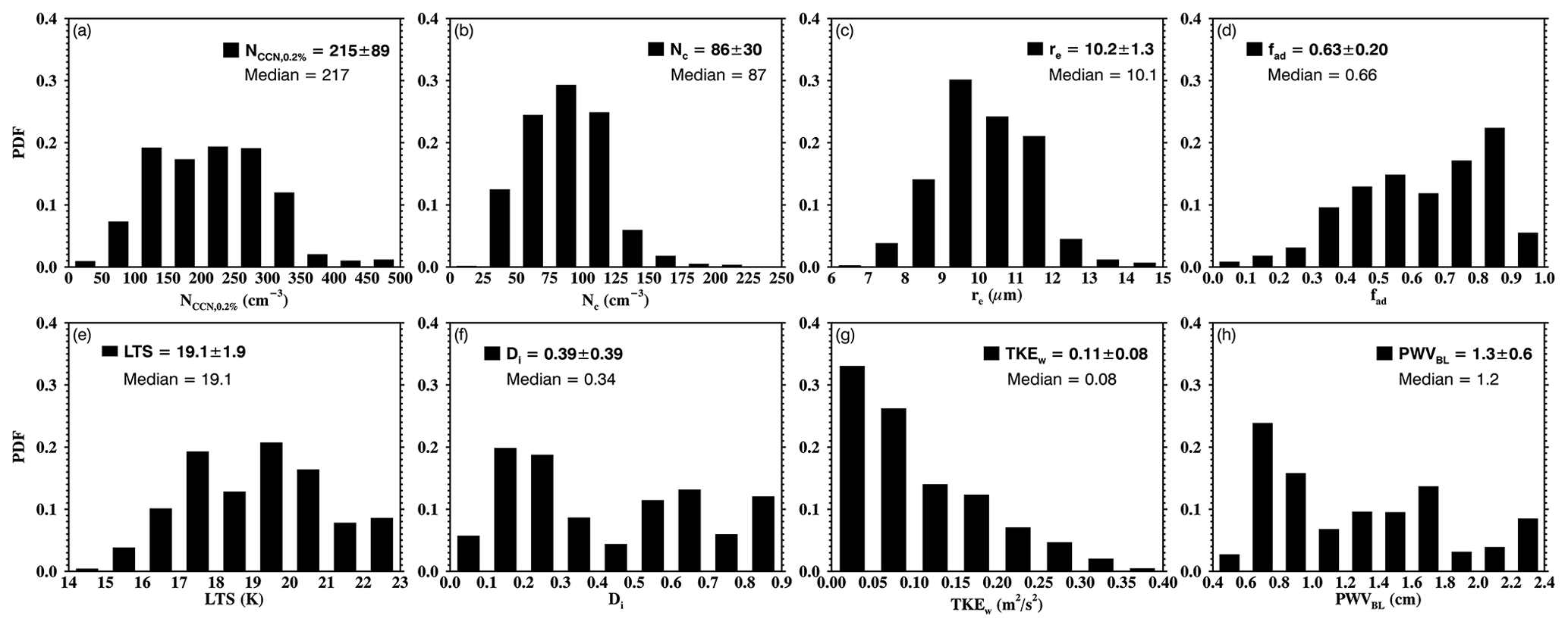
Figure 1 Probability distribution functions (PDFs), mean, standard deviation, and median values of aerosol, cloud, and meteorological properties for 20 selected non-precipitating cloud cases at the DOE ENA site during the period 2016–2018. (a) Cloud condensation nuclei (CCN) number concentration at 0.2 % supersaturation (N_CCN,0.2 %); (b) cloud droplet number concentration (N_c); (c) cloud droplet effective radius (r_e); (d) cloud adiabaticity (f_ad); (e) lower tropospheric stability (LTS); (f) decoupling index (D_i); (g) mean vertical component of turbulence kinetic energy (TKE_w); (h) sub-cloud boundary layer precipitable water vapor (PWV_BL).

The probability distribution functions (PDFs) of the aerosol and cloud properties and the environmental conditions for the selected cases are shown in Fig. 1. The PDF of N_CCN,0.2 % presents a normal distribution with a mean value of 215 cm⁻³ and median value of 217 cm⁻³. About 97 % of the N_CCN,0.2 % samples lie below 350 cm⁻³ and represent a relatively clean environment (Logan et al., 2014, 2018). A few instances of aerosol intrusions (∼ 3 %) with higher N_CCN,0.2 % were likely a result of continental air mass transport from North America, Europe, and Africa (Logan et al., 2014; Wang et al., 2020). As for the cloud microphysical properties, the cloud-layer-mean N_c and r_e (Fig. 1b and c) are also both normally distributed with median values close to the mean values. The majority of the N_c values (∼ 91 %) are lower than 125 cm⁻³ with a mean value of 86 cm⁻³, and the r_e distribution peaks between 9–11 µm with a mean value of 10.1 µm. Both N_c and r_e values fall in the typical ranges of the non-precipitating MBL cloud characteristics over the ENA site (Dong et al., 2014; Wu et al., 2020b). The distribution of f_ad is slightly skewed to the left with a median value of 0.66 (Fig. 1d), indicating that the bulk of cloud samples are close to adiabatic environments, while the left tail denotes a wide range of cloud sub-adiabaticities, which allows us to investigate the role of cloud adiabaticities in the cloud microphysical variations.

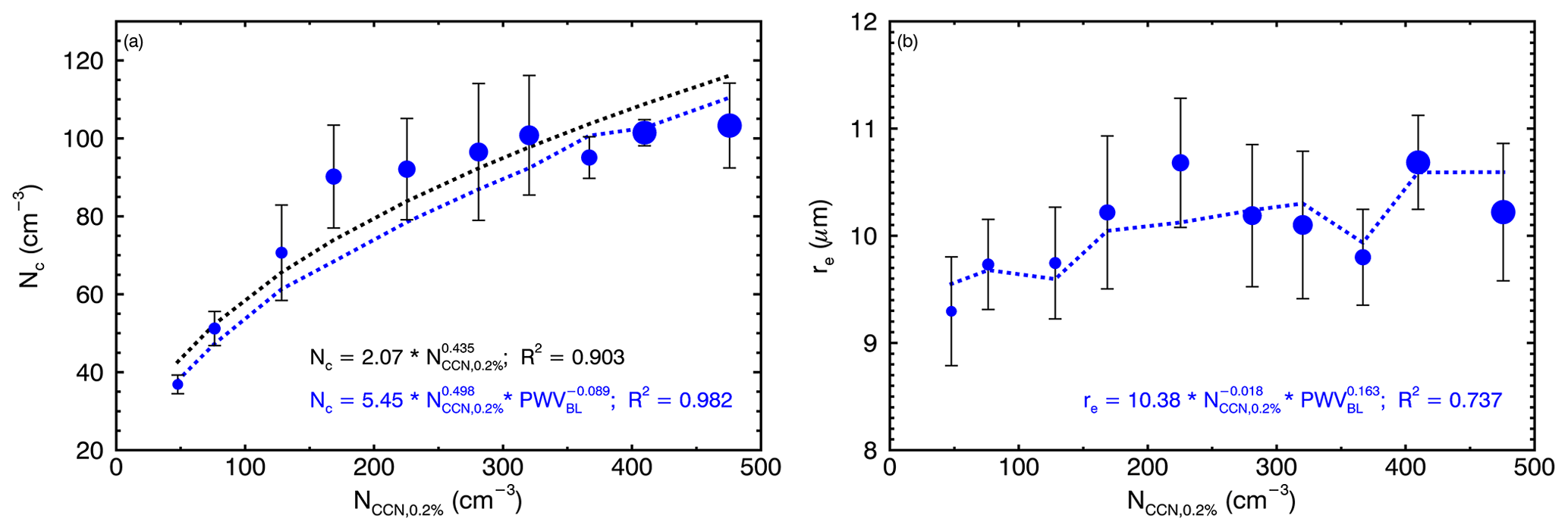
Figure 2 (a) N_c and (b) r_e as a function of N_CCN,0.2 % (x axis) and PWV (filled blue circles) for all selected samples. The larger blue circles represent higher PWV values. Whiskers denote 1 standard deviation for each bin.

For all selected cases, the LTS, which represents the large-scale thermodynamic structure, is distributed bimodally across the range from 14 to 23 K with mean and median values of 19.1 K in Fig. 1e. A higher LTS magnitude represents a relatively stable environment and is favorable to the formation of marine stratocumulus (Medeiros and Stevens, 2011; Gryspeerdt et al., 2016). Note that the median LTS of 19.1 K in this study is close to the separation threshold of 18.55 K suggested by prior studies to distinguish the marine stratocumulus from a global assessment of marine shallow cumulus clouds (Smalley and Rapp, 2020). Therefore, leveraging the demarcation line at 19.1 K may allow us to investigate the aerosol–cloud relationships under contrasting thermodynamic regimes. The PDF of the D_i parameter spreads widely with a median value of 0.34 for the selected cases (Fig. 1f), which provides an opportunity to study the cloud sample behaviors under MBL conditions ranging from well-mixed to decoupled. Higher D_i values indicate a more decoupled MBL with weaker turbulence which cannot sufficiently maintain the well-mixed MBL, while lower D_i values are often associated with stronger turbulence which maintains a coupled MBL (Jones et al., 2011). As an indicator of the below-cloud boundary layer turbulence, the TKE_w values present a gamma distribution that is highly skewed to the right (Fig. 1e), with a mean value of 0.11 and a median value of 0.08 m² s⁻². About half of the cloud samples are observed within a less turbulent environment (which is also implied by the higher half of D_i), suggesting weak connections between the cloud layer and the below-cloud boundary layer. The other half of the cloud samples, with higher TKE_w values up to 0.4 m² s⁻², implies tighter connections between cloud microphysical properties and the below-cloud boundary layer accompanied by intensive turbulent conditions, which is favorable to enhancing cloud droplet growth (Albrecht et al., 1995; Hogan et al., 2009; Ghate et al., 2010; West et al., 2014; Ghate and Cadeddu, 2019).

It is noteworthy that PWV_BL values exhibit a bimodal distribution with a median value of 1.2 cm (Fig. 1f). About 49 % of the samples have their PWV_BL values in the range of 0.4–1.2 cm with the first peak at 0.6–0.8 cm, and 51 % of the samples have PWV_BL values higher than 1.2 cm with a second peak at 1.6–1.8 cm, which may be due to the seasonal difference in the selected cases. Figure S2 in the Supplement shows the seasonal variation in the PWV_BL from 2016 to 2018 when single-layered low clouds are present. The monthly PWV_BL values are as low as ∼ 0.9 cm and remain nearly invariant from January through March, then increase to ∼ 2.0 cm (doubled) in September, and decrease dramatically toward the winter months. The selected cloud cases are distributed across the seasons, with ∼ 34 % of the samples occurring during the months with the lowest mean PWV_BL (January–March), while ∼ 43 % of the samples fall in the highest-PWV_BL months (June–September). These two different PWV_BL regions will provide a great opportunity for us to further examine the ACI under lower and higher water vapor conditions.

3.2 Dependence of cloud microphysical properties on CCN and PWV_BL

Figure 2 shows the cloud microphysical properties as a function of N_CCN,0.2 % and PWV_BL for the samples from 20 selected cases. As illustrated in Fig. 2a, there is a statistically significant positive correlation (R² = 0.9) between ln (N_c) and ln (N_CCN,0.2 %). The linear fit of ln (N_c) to ln (N_CCN,0.2 %) is then mathematically transformed to a power-law fitting function of N_c to N_CCN,0.2 % and plotted as dashed lines in Fig. 2a. The power-law fitting indicates that 90.3 % of the variation in binned ln (N_c) can be explained by the change in the binned ln (N_CCN,0.2 %) and further suggests that with more available below-cloud CCN, higher number concentrations are expected. The logarithmic ratio $\partial \ln \left({\mathit{\text{N}}}_{\mathrm{c}}\right)/\partial \ln \left({\mathit{\text{N}}}_{\mathrm{CCN},\mathrm{0.2}\mathrm{\%}}\right)$ is computed to be 0.435 from our study. This ratio is very close to 0.48 as was shown by McComiskey et al. (2009), who also used ground-based measurements to study the marine stratus clouds over the California coast. The logarithmic ratio (0.435) is also close to the result (0.458) of Lu et al. (2007), who used aircraft in situ-measured cloud droplet and accumulation-mode aerosol number concentration for the marine stratus and stratocumulus clouds over the eastern Pacific Ocean. The ratio reflects the relative conversion efficiency of cloud droplets from the CCN, regardless of the water vapor availability. Theoretically, it has the boundaries of 0–1, where the lower bound means no change in N_c with N_CCN and the upper bound indicates a linear relationship where every cloud condensation nucleus would result in one cloud droplet. Our result is comparable with the previous studies targeting the MBL stratiform clouds, indicating a certain similarity of the bulk cloud microphysical responses with respect to aerosol intrusion in those types of cloud and over different marine environments and further supporting that the assessment in this study is valid.

The PWV_BL values are represented as blue circles (larger one for higher PWV_BL) in Fig. 2a in order to study the role of water vapor availability in the CCN–N_c conversion process. As demonstrated in Fig. 2a, the PWV_BL values almost mimic the increasing N_CCN,0.2 % trend, which is also governed by the seasonal N_CCN,0.2 % and the selected cloud cases. Figure S3 in the Supplement shows the seasonal variation in N_CCN,0.2 % from 2016 to 2018. It is noticeable that the monthly N_CCN,0.2 % values, which mimic the monthly variation in PWV_BL, are much higher during warm months (May–October) than during cold months (November–April). This seasonal N_CCN,0.2 % variation has also been found in recent studies of MBL aerosol composition and number concentration. During the warm months, the below-cloud boundary layer is enriched by the accumulation mode of sulfate and organic particles via local generation and long-range transport induced by the semi-permanent Azores High; these particles are found to be hydrophilic and can be great CCN contributors (Wang et al., 2020; Zawadowicz et al., 2020; Zheng et al., 2018; G. Zheng et al., 2020). Therefore, the coincidence of high N_CCN,0.2 % and PWV_BL does not necessarily imply a physical relationship but instead is the result of their similar seasonal trend. The potential co-variabilities between N_CCN,0.2 % and PWV_BL and hence the implication for the N_c variation will be further investigated in Sect. 3.5. When taking the PWV_BL into account, R² increases from 0.903 to 0.982, and this new relationship suggests that the co-variability between the binned ln (N_CCN,0.2 %) and ln (PWV_BL) has a stronger correlation with the change in binned ln (N_c). Intuitively, if the CCN–N_c relationship is primarily dominated by the diffusion of water vapor, more CCN and higher PWV_BL should result in a continuous increase in N_c. However, the rapid increase in N_c (37 to 92 cm⁻³) in the first half of N_CCN,0.2 % bins (< 250 cm⁻³) does not happen in the second half of the N_CCN,0.2 % bins (> 250 cm⁻³), where the slope of the N_c increase (96 to 103 cm⁻³) appears to be flattened for higher N_CCN,0.2 % and PWV_BL bins. Furthermore, the joint power-law fitting of N_c (to N_CCN,0.2 % and PWV_BL) appears to be constantly lower than the single power-law fitting of N_c (to N_CCN,0.2 % solely) in each bin. The negative power of PWV_BL in this relationship suggests that PWV_BL might play a stabilization role in the diffusional growth process, which will be further analyzed in the following sections.

The relationship between r_e and N_CCN,0.2 % is shown in Fig. 2b, where there is no significant relationship between r_e and N_CCN,0.2 % solely, given a near-zero slope and the low correlation coefficient (fitted line not plotted). However, after applying a multiple linear regression to the logarithmic form of r_e, N_CCN,0.2 %, and PWV_BL, a significant correlation among those three variables is found. The r_e is negatively correlated with N_CCN,0.2 % and positively correlated with PWV_BL, and 73.7 % of the variations in binned ln (r_e) can be explained by the joint changes in the binned ln (N_CCN,0.2 %) and ln (PWV_BL). This indicates that in the bulk part, r_e decreases with increasing N_CCN,0.2 % and enlarges with increasing PWV_BL. Notice that in the lower N_CCN,0.2 % bins (< 150 cm⁻³) where the PWV_BL values are the lowest among all the bins (0.76–0.85 cm), the limitation of cloud droplet growth by competing for the available water vapor is evident by the changes in N_c and r_e. For example, N_CCN,0.2 % changes from 47 to 128 cm⁻³, N_c increases from 37 to 71 cm⁻³, and r_e only increases from 9.30 to 9.74 µm. In other words, nearly tripling the CCN loading leads to roughly doubling N_c, while the r_e is only enlarged by 0.44 µm (4.7 %). In the relatively low available PWV_BL regime, it is clear that even with more CCN being converted into cloud droplets, the limited water vapor condition prohibits the further diffusional growth of those cloud droplets. However, in the higher N_CCN,0.2 % bins (> 150 cm⁻³) with higher PWV_BL, the binned r_e values fluctuate and decrease with increasing CCN bins under similar PWV_BL values (i.e., the two N_CCN,0.2 % ranges from 200–400 cm⁻³ and from 400–500 cm⁻³). Since r_e essentially represents the area-weighted information of the cloud droplet size distribution (DSD), this sorting method of r_e inevitably entangles multiple cloud droplet evolution processes and environmental effects that can alter the DSD, especially under the condition of sufficient water supply. Therefore, the further assessment of the r_e responses to the N_CCN,0.2 % loading under the constraint of water vapor should be discussed in order to untangle the impacts of different processes and environmental effects on r_e.

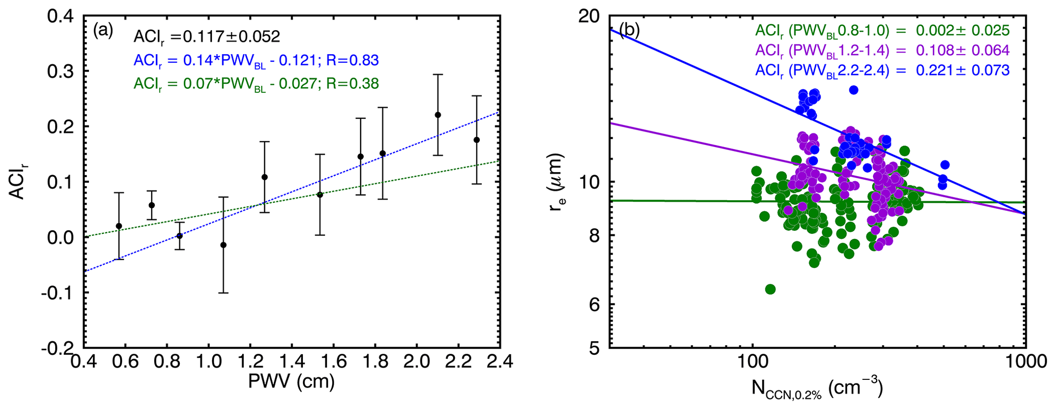
Figure 3 (a) Relationship of ACI_r (dots) to binned PWV_BL. Whiskers denote 1 standard deviation for each bin. Linear regressions are performed in a relatively low PWV_BL regime (< 1.4 cm, green) and high-PWV_BL regime (> 1.4 cm). (b) Illustration of ACI_r derived from r_e against N_CCN,0.2 % in the following three PWV_BL bins: 0.8–1.0 cm (green), 1.2–1.4 cm (purple), and 2.2–2.4 cm (blue). ACI_r represents the relative change in r_e with respect to the relative change in N_CCN,0.2 %, where positive ACI_r denotes the decrease in r_e with increased N_CCN,0.2 % under binned PWV.

3.3 Aerosol–cloud interaction under different water vapor availabilities

As previously discussed above and suggested by earlier studies, the conditions of water vapor supply have a substantial impact on various processes from CCN–N_c conversion to in-cloud droplet condensational growth and coalescence processes, hence effectively altering the cloud DSD (Feingold et al., 2006; McComiskey et al., 2009; X. Zheng et al., 2020). Moving forward to examine how r_e responds to the changes in N_CCN,0.2 % in the context of a given water vapor availability, an index describing the aerosol–cloud interaction process is introduced as follows:

$$\begin{array}{}\text{(3)}& {\mathrm{ACI}}_{\mathrm{r}}={\left.-{\displaystyle \frac{\partial \ln \left(r_{\mathrm{e}}\right)}{\partial \ln \left({\mathit{\text{N}}}_{\mathrm{CCN},\mathrm{0.2}\mathrm{\%}}\right)}}\right|}_{{\mathrm{PWV}}_{\mathrm{BL}}}.\end{array}$$

ACI_r represents the relative change in r_e with respect to the relative change in N_CCN,0.2 %, where positive ACI_r denotes the decrease in r_e with increasing N_CCN,0.2 % under binned PWV_BL. This assessment of ACI_r focuses on the relative sensitivity of the cloud microphysics response in the stratified water vapor environment, while previous studies used the cloud liquid water path (LWP) as the constraint (Twomey, 1977; Feingold et al., 2003; Garrett et al., 2004). The LWP describes the liquid water (i.e., existing cloud droplets) physically linked to r_e and N_c, which have an interdependent relationship in cloud retrieval procedures and hence, to a certain extent, share co-variabilities with cloud microphysical properties (Dong et al., 1998; Wu et al., 2020a). In this study, by using the PWV as a sorting variable, we are trying to capture the role of ambient available water vapor in the cloud droplet growth process (especially the water vapor diffusional growth), using measurement independent of the cloud retrievals. Figure 3 shows the variation in ACI_r under different PWV_BL bins and illustrates the calculation of ACI_r in three different PWV_BL ranges. Note that in Fig. 3a, the regressions are derived from all points (statistically significant with a confidence level of 95 %). As shown in Fig. 3a, the ACI_r values range from close-to-zero values (−0.01) to 0.22, with the mean value of 0.117 ± 0.052. The ACI_r range of this study agrees well with the previous studies of MBL cloud aerosol–cloud interactions (McComiskey et al., 2009; Pandithurai et al., 2009; Liu et al., 2016). It is noteworthy that the variation in ACI_r with PWV_BL suggests two different relationships under separated PWV_BL conditions, as discussed in the following two paragraphs.

Under the lower PWV_BL condition (< 1.2 cm), the low values of ACI_r (−0.01–0.057) indicate that r_e is less sensitive to N_CCN,0.2 %, and the dependence on PWV_BL is also insignificant as given by the flat regression line (dashed green line) and low correlation coefficient of 0.38 (Fig. 3a). As discussed in Sect. 3.2, the limited water vapor can weaken the ability of condensational growth of the cloud droplet converted from CCN; that is, the increase in CCN loading cannot be effectively reflected by a decrease in r_e. For example, a 307 % increase in N_CCN,0.2 % only leads to a 10 % decrease in r_e in the PWV_BL range of 0.8–1.0 cm as shown in Fig. 3b. So in this regime, even with a slight PWV_BL increase, the lack of a sufficient number of large cloud droplets is favorable to the predominant condensational growth process, which effectively narrows the cloud DSD and, in turn, confines the variable range of r_e with respect to N_CCN,0.2 % (Pawlowska et al., 2006; G. Zheng et al., 2020). In this situation, the ability of CCN to be converted to cloud droplets as well as droplet condensational growth is limited by insufficient water vapor, rather than by an influx of CCN.

Table 2 Occurrence frequencies of large in-cloud r_e^∗ under relatively high PWV conditions.

^∗ The occurrence of large r_e is defined when the r_e is found to be larger than 12 or 14 µm using the retrieved in-cloud vertical profiles.

However, under the higher-PWV_BL regime (> 1.2 cm), the ACI_r values become more positive and express a significant increasing trend with PWV_BL (correlation coefficient of 0.83, dashed blue line), which indicates that r_e is more susceptible to N_CCN,0.2 % in this regime. On the one hand, due to the sufficient water vapor supply, the enhanced condensational growth process allows more CCN to grow into cloud droplets, so the limiting factor of the droplet growth corresponds to the changes in CCN loading. On the other hand, the increased N_c values associated with higher water vapor supply in the cloud effectively enhance the coalescence process. This results in broadening the cloud DSD and increasing the variation range of r_e in response to the changes in N_CCN,0.2 %. To test our hypothesis of active coalescence under higher water vapor conditions, Table 2 lists the occurrence frequencies of large r_e values (> 12 and 14 µm) under the six high PWV_BL bins (1.2–2.4 cm), because this range of 12–14 µm can serve as the critical demarcation of an efficient coalescence process (Gerber, 1996; Freud and Rosenfeld, 2012; Rosenfeld et al., 2012). As listed in Table 2, for the six high PWV_BL bins, the occurrence frequencies of r_e > 12 µm are 25.0 %, 30.6 %, 54.1 %, 74.2 %, 93.8 %, and 97.5 % and the occurrence frequencies of r_e > 14 µm are 1.25 %, 1.77 %, 7.4 %, 17.7 %, 31.9 %, and 20.1 %.

The increasing trends of large-r_e occurrences mimic the trend of ACI_r and suggest that with increased PWV_BL, cloud droplets have a greater chance to grow via the effective coalescence process and subsequently lead to an enlargement of ACI_r. Although previous studies have brought up the potential impacts of the cloud droplet coalescence process on ACI, the relationship among them has rarely been discussed in detail. Here we provide possible explanations for how the enhanced coalescence process can enlarge ACI_r. Quantitatively, ACI_r is described by the logarithmic partial derivative ratio of r_e to N_CCN,0.2 %; thus a sharper decrease in r_e with respect to a given N_CCN,0.2 % range can result in a steeper slope and, in turn, larger ACI_r (i.e., a 239 % increase in N_CCN,0.2 % leads to an r_e decrease of 48 % in the 2.2–2.4 cm bin in Fig. 3b). Physically, this relies on how the cloud droplet size distribution (DSD) would change with different CCN loadings. Therefore, particularly in low CCN conditions, sufficient water vapor availability will allow cloud droplets to continuously grow via diffusion of water vapor (i.e., condensational growth) and enter the active cloud droplet coalescence regime. In contrast, the increase in cloud droplet size can effectively reduce N_c via the process of large cloud droplets collecting small droplets, and small droplets coalescing into large droplets. Consequently, the cloud DSD becomes effectively broadened toward the large tail by the coalescence so that r_e is enlarged. With more CCN available, the cloud DSD is narrowed by the enhanced condensational growth and regresses toward the small tail by increasing the number of newly converted cloud droplets which result in decreased r_e. These interactions between CCN and cloud droplets ultimately result in the broadened changeable range of r_e and, in turn, the enlarged ACI_r.

Table 3 ACI_r calculated with respect to N_CCN theoretically at different supersaturation levels, under all PWV_BL conditions.

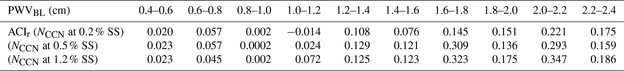
In order to investigate the theoretical implication of supersaturation conditions for the aerosol–cloud interaction observed here in the MBL stratiform clouds, the ACI_r values are calculated with respect to the surface N_CCN theoretically at two additional high supersaturation levels (0.5 % and 1.2 %), under all PWV_BL conditions. The results in Table 3 show that the ACI_r signals both are weak and do not have significant changes under lower PWV_BL conditions, while the ACI_r signals tend to strengthen with the increase in supersaturation under the higher PWV_BL. Based on Köhler theory, if the supersaturation exceeds the critical point for the given droplet, the droplet will thus experience continued growth, so theoretically the ACI should increase with the supersaturation under the same aerosol number concentration. However, the observed limited water vapor cannot support this ideal droplet growth, resulting in weak responses of cloud droplets to aerosol intrusion. With the increase in observed water vapor, the continued growth of cloud droplets becomes more plausible; hence the high supersaturation yields larger droplets with a low number of aerosols; more efficient droplet activation with a large number of aerosols; and, in turn, larger ACI_r (even out of the theoretical bounds). However, considering that these high-supersaturation environments are unphysical in the observed MBL cloud layers and estimating the real supersaturation conditions using ground-based remote sensing is beyond the scope of this study, we chose the supersaturation level of 0.2 % because it represents the most typical supersaturation conditions of MBL stratiform clouds.

3.4 The co-variabilities of the meteorological factors

The environmental conditions over the ENA have been widely studied as not independent but entangled with each other (Wood et al., 2015; Zheng et al., 2016; Wu et al., 2017; Wang et al., 2021). To better understand the dependencies and the co-variabilities of the meteorological factors, a principal component analysis (PCA) is performed comprising the following variables: (1) PWV_BL denotes the water vapor availability within the boundary layer; (2) D_i describes the boundary layer coupling conditions; (3) TKE_w represents the strength of boundary layer turbulence; (4) W_dir,NS reflects the surface wind directions in terms of northerly and southerly; (5) LTS implies the large-scale thermodynamic structures. Note that the W_dir,NS values are taken as W_dir,NS = $\text{abs}(W_{\text{dir}}-\mathrm{180}{}^{\circ }$), so the original W_dir (0–360^∘) can be transformed to W_dir,NS (0–180^∘) where the values smaller than 90^∘ are close to the southerly wind and those greater than 90^∘ are close to the northerly wind. The W_dir,NS values are transformed as such to capture the island effects better because the cliff is located north of the ENA site.

The input data metric of the PCA is constructed from the above five variables; thus the principal components (PCs) that explain the variations in those dependent variables can be output from the eigenanalysis. The result shows that for the five selected meteorological factors, the proportions of the total intervariable variance explained by the PCs are 43.72 %, 22.01 %, 18.26 %, 8.95 %, and 7.06 % and the eigenvalues are 2.19, 1.10, 0.91, 0.45, and 0.35, respectively. Note that the first three PCs have the highest eigenvalues and explain most (∼ 84 %) of the total variance, which indicates that they can capture the significant variation patterns of the selective meteorological factors.

Table 4 The first three principal components from eigenanalysis.

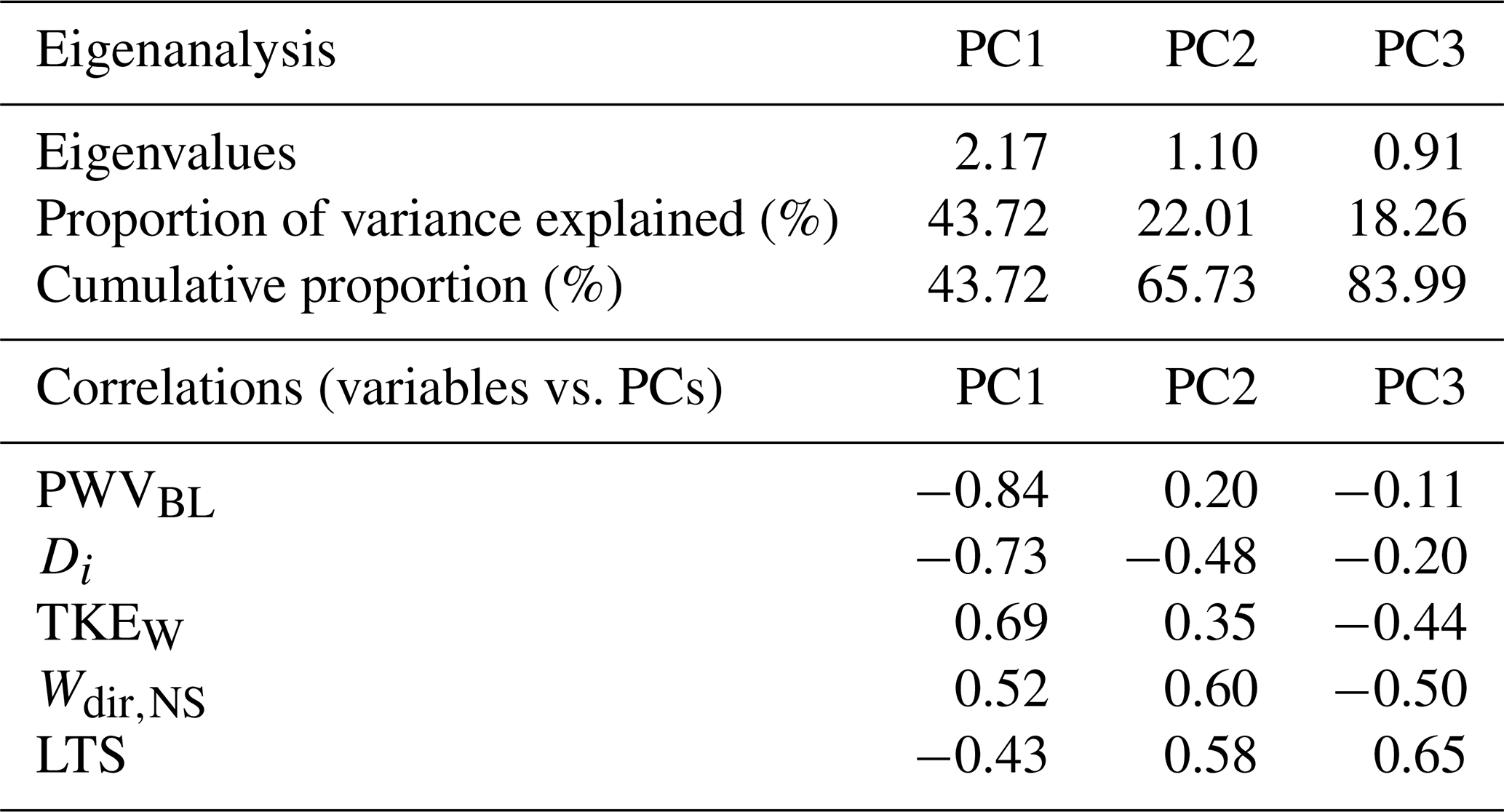
To determine the relative contributions of the variables to PCs, all the five selected meteorological variables are projected to the first three PCs, and the Pearson correlation coefficients between them are listed in Table 4. For the first PC (PC1), which accounts for the highest proportion (43.72 %) of the total variance, the PC1 is strongly negatively correlated with PWV_BL (−0.84) and D_i (−0.73) but strongly positively correlated with TKE_w (0.69). These results suggest that PC1 mainly represents the boundary layer conditions, and the co-variations in the boundary layer water vapor and turbulence are the most distinct environmental patterns for the selected cloud cases. PC2 and PC3 are most correlated with LTS (0.58 and 0.65 for PC2 and PC3, respectively) and W_dir,NS (0.60 and −0.50 for PC2 and PC3, respectively), indicating that PC2 and PC3 mainly describe the variations in large-scale thermodynamics and the surface wind patterns, which are likely associated with the variations in the Azores High position and strength (Wood et al., 2015).

Figure 4 The projections of TKE_w (purple), W_dir,NS (red), LTS (orange), PWV_BL (blue), and D_i (green) onto the first principal component (PC1) and the second principal component (PC2). The x coordinates denote variables' correlations with PC1, and the y coordinates denote variables' correlations with PC2.

To further understand the correlations between the meteorological variables, the principal component loading plot is constructed by projecting the variables onto PC1 and PC2 as shown in Fig. 4. Each point denotes the variable correlations with PC1 (x coordinate) and PC2 (y coordinate) so that each vector represents the strength and direction of the original variable influences on the pair of PCs. The angle between the two vectors represents the correlation between them. In Fig. 4, both TKE_w and W_dir,NS vectors are located in the same quadrant (positive in both PC1 and PC2) and close to each other with a small degree of an acute angle, which means the TKE_w values are strongly correlated with W_dir,NS. If the surface wind were coming from the north side of the island, the topographic lifting effect of the cliff would induce additional updraft over the ENA site (Zheng et al., 2016), so the wind closer to the northerly wind (larger W_dir,NS) is more correlated with higher TKE_w. Note that the TKE_w and D_i vectors are almost in an opposite direction to each other, which denotes a strongly negative correlation between the two variables. The angles of PWV_BL with D_i (∼ 45^∘) and TKE_w (∼ 142^∘) suggest that PWV_BL is moderately positively correlated with D_i but negatively correlated with TKE_w. A higher D_i indicates a more decoupled MBL, where MBL is not well-mixed and separated into a radiative-driven layer and a surface-flux-driven layer that caps the surface moisture (Jones et al., 2011). This situation is more likely to be associated with a higher PWV_BL and weaker TKE_w condition. Note that the negative correlation between D_i and TKE_w examined here might also be partly attributed to the diurnal cycle of the turbulence, which is suggested to be associated with the cloud-top longwave radiative cooling over the ENA, especially for the drizzling clouds (Ghate et al., 2021; Zheng et al., 2016). However, this study focuses on the non-precipitating clouds where the effect of drizzle on the cloud-top radiative-cooling-driven turbulence is minimal, and examining the cloud-top radiative cooling rate from ground-based remote sensing is beyond the scope of the current study. It would be of interest to obtain the accurate cloud-top radiative cooling rate using a radiative transfer model in the future. As for the LTS parameter, the close-to-90^∘ angle with TKE_w suggests no correlation between them, since the LTS mostly captures the large-scale thermodynamical structures and is obtained from a coarser temporal resolution. Thus, the LTS does not essentially correspond to the strength of boundary layer turbulence and can be treated as independent of TKE_w over the ENA site. The loading plot intuitively tells us the directions and strengths of the co-variabilities of the selected meteorological variables and sheds light on determining the key factors that are feasible to use in examining the environmental impacts on the aerosol–cloud interactions.

3.5 Linking the meteorological factors to aerosol–cloud interaction

3.5.1 Relations of meteorological factors with aerosol and cloud properties

The PCs are, mathematically, the linear combination of the selected variables and hence independent of each other after the PCA. Therefore, treating the aerosol and cloud properties as dependents and correlated with the PCs allows us to infer their co-variation with the meteorological factors statistically. A weakly negative correlation between N_CCN,0.2 % and PC1 (R_PC1,CCN = −0.35) suggests that the higher N_CCN,0.2 % could sometimes be found under higher PWV_BL and lower TKE_w. Though the correlation is low, the plausible contributions could come from the seasonal variations in N_CCN,0.2 % and PWV_BL as discussed in the previous section, and the weaker TKE_w might prevent the vertical mixing of CCN and induce higher surface N_CCN,0.2 %. On the other hand, a weakly positive correlation between N_CCN,0.2 % and PC2 (R_PC2,CCN = 0.21) suggests that there are no fundamental relationships between CCN with thermodynamics and the surface wind direction, and they are not the key controlling factor of surface N_CCN,0.2 % variation because the surface CCN concentration is primarily contributed by the accumulation-mode aerosols which come from the condensational growth of Aitken-mode aerosols (Zheng et al., 2018). As for the cloud properties, both N_c and f_ad are negatively correlated with PC1 ($R_{\text{PC1},N_{\mathrm{c}}}$ =  −0.51 and R_PC1,fad = −0.62, respectively), suggesting a moderate relationship between N_c, f_ad, and the boundary layer condition. These negative correlations suggest that under the higher PWV_BL condition, the sufficient water vapor supply allows more CCN to become cloud droplets, as previously discussed, and hence increases the cloud adiabaticity due to the dominant condensational growth process. While in the situation of higher TKE_w, the decrease in the N_c and f_ad might be partly attributed to the association with the active in-cloud coalescence process and entrainment of dry air. However, owing to the obstacle of retrieving in-cloud TKE_w from the ground-based remote sensing, the usage of sub-cloud TKE_w in this study captures part of the relationship between turbulence and adiabaticity. Therefore, in this situation, the cloud adiabaticity might depend more on PWV_BL and the boundary layer decoupling state. Moreover, their low correlations with PC2 ($R_{\text{PC2},N_{\mathrm{c}}}$ = −0.10 and R_PC2,fad = −0.17, respectively) indicate very weak relations with the large-scale thermodynamic variables. These weak correlations are likely to be due to the subset of MBL single-layer stratocumulus in this study, as the previous study over the ENA found that the sensitivity of MBL cloud adiabaticity largely depends on the strength of cloud-top inversion (which can be partially indicated by the increased LTS) and slightly depends on the boundary layer decoupling (Terai et al., 2019; Y. Zheng et al., 2020). Note that the same sign of correlations with PC1 statistically infer a similar directional co-variation in N_CCN,0.2 %, N_c, and f_ad to a certain extent.

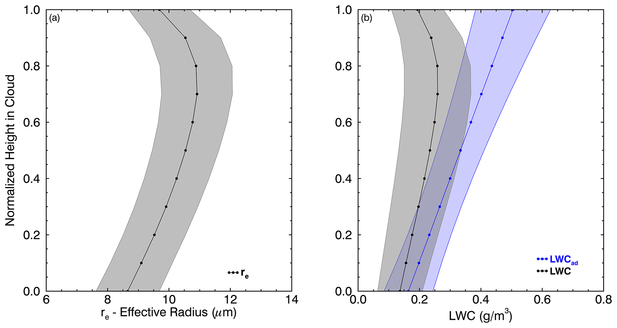
Figure 5 Normalized in-cloud vertical profiles of retrieved (a) r_e and (b) LWC (black) and calculated adiabatic LWC_ad (blue) for all selected cloud cases; 0 is cloud base, and 1 is cloud top. Solid lines with dots denote mean values, and shaded areas denote 1 standard deviation at each height.

To examine the physical relation between N_CCN,0.2 %, N_c, and f_ad, the profiles of cloud r_e and LWC are plotted at normalized height from the cloud base (z_b) to cloud-top height (z_t) (Fig. 5), which is given by $z_{\mathrm{n}}=(z-z_{\mathrm{b}})/(z_{\mathrm{t}}-z_{\mathrm{b}}$). The solid lines denote the mean values, and the shaded area represents 1 standard deviation at each normalized height z_n. The normalized r_e increases from ∼ 8.6 µm at the cloud base toward ∼ 11 µm near the upper part of the cloud where z_n is 0.7 (Fig. 5a), through condensational growth and coalescence processes, and then decreases toward the cloud top due to cloud-top entrainment. Similar in-cloud vertical variation in r_e is also found in previous studies using aircraft in situ measurements (Zhao et al., 2018; Wu et al., 2020a). Profiles of retrieved LWC and calculated adiabatic LWC_ad (blue line) are presented in Fig. 5b. As demonstrated in Fig. 5b, the f_ad values, which are the ratio of LWC to LWC_ad, reach a maximum of 0.8 at the cloud base and a minimum of 0.38 at the cloud top. The shaded areas of r_e and LWC denote the range from near-adiabatic to sub-adiabatic cloud environments, where in the near-adiabatic cloud (higher f_ad) the cloud droplets experience adiabatic growth and LWC should be close to LWC_ad. In contrast, in the sub-adiabatic cloud regime, the decrease in f_ad is largely due to cloud-top entrainment and coalescence processes even in non-precipitating MBL clouds (Wood, 2012; Braun et al., 2018; Wu et al., 2020b). Furthermore, to understand the implication of cloud adiabaticity with respect to CCN–N_c conversion, all of the f_ad samples are separated into two groups by the median value of the layer-mean f_ad (0.66) for further analysis.

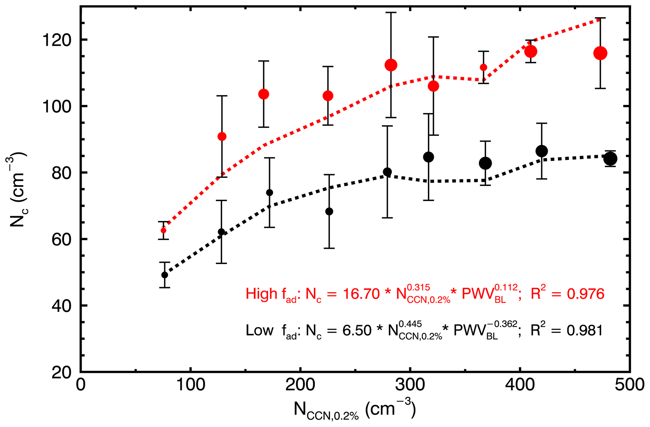
Figure 6 N_c as a function of N_CCN,0.2 % (x axis) and PWV (dots) for high-adiabaticity (high-f_ad) (red) and low-f_ad (black) regimes. The larger circles represent higher PWV values. Whiskers denote 1 standard deviation for each bin.

Figure 6 shows N_c against the binned N_CCN,0.2 % for the near-adiabatic regime (f_ad > 0.66) and sub-adiabatic regime (f_ad < 0.66). For the near-adiabatic regime, N_c increases from ∼ 60 to 119 cm⁻³ with increased N_CCN,0.2 % and PWV_BL, and both N_CCN,0.2 % and PWV_BL appear to play positive roles in terms of the N_c increase. The result is as expected because the process of condensational growth is predominant in the near-adiabatic clouds; that is, with increasing water vapor supply, the higher CCN loading can effectively lead to more cloud droplets. However, in the sub-adiabatic cloud regime, N_c increases with increased N_CCN,0.2 % but possesses a negative correlation with PWV, which results in a slower increase in N_c under higher N_CCN,0.2 % and PWV_BL conditions. The mean reduction in N_c in the sub-adiabatic regime is computed to be ∼ 37 % compared to that for the near-adiabatic clouds. As previously studied, the coalescence process contributes significantly to N_c depletion, even in non-precipitating MBL clouds (Feingold et al., 1996; Wood, 2006). Thus, lower N_c in the sub-adiabatic regime may be partly due to the combined effect of coalescence and entrainment (Wood, 2006; Hill et al., 2009; Yum et al., 2015; Wang et al., 2020). Note that the retrieved N_c represents the cloud-layer-mean information. In summary, the Wu et al. (2020a) retrieval works to separate the reflectivity into the contributions of cloud (Z_c) and drizzle. The retrieval assumes an initial guess of the representative layer-mean N_c based on the climatology over ENA sites (Dong et al., 2014) and as such allows the first guess of the vertical profile of LWC based on N_c and Z_c, then constrains the N_c and LWC using the LWP derived from MWR, and finally outputs r_e values (Fig. 3 in Wu et al., 2020a). Therefore, the final retrieved N_c is updated in response to the cloud microphysical processes within this time step. From the aircraft in situ measurements during the ACE-ENA, we found that the observed vertical profile of N_c is near constant in the middle part of the cloud (even in the drizzling cloud where the collision–coalescence processes are more active), and the signal of entrainment-induced N_c depletion is shown near the cloud top (Wu et al., 2020a). However, it is difficult and beyond the scope of the ground-based retrieval to compare the vertical dependency of the depletion rate within one time step. Therefore, as the retrieval currently works to represent the layer-mean information from the given time step, the preferred method in this study is to compare N_c values at different times, which in this case correspond to the adiabatic versus sub-adiabatic conditions, which hence yield different N_c values that we retrieved from the ground-based snapshot perspective. From the PCA and binning analysis, the effect of cloud adiabaticities on CCN–N_c conversions may shed light on interpreting the aerosol–cloud interaction under different environmental effects.

3.5.2 The role of meteorological factors in ACI_r assessment

Since ACI_r can only be calculated by the logarithmic derivatives from a set of N_CCN,0.2 % and r_e data within a certain regime, it will be inappropriate to linearly correlate the data with PCs directly, from both mathematical and physical perspectives. Therefore, the meteorological factors which have the strongest influence on the most explanatory PCs, namely PWV_BL and TKE_w, are selected to be the sorting variables in assessing the environmental impacts on the ACI_r. In addition, LTS is also selected as it represents the large-scale thermodynamic factor and is independent of the boundary layer environment conditions. The data samples are first separated into two regimes using the median values of the targeting factors and then separated into four quadrants by the median PWV_BL because ACI_r is found to have significant differences under different water vapor availabilities. The ACI_r values are further calculated for all quadrants to examine whether the ACI_r can be distinguished by the targeting factors.

Combining LTS and PWV_BL as sorting variables, the ACI_r values for four regimes are shown in Fig. S4 in the Supplement. The ACI_r differences between low- and high-PWV_BL regimes are still retained. In the low-PWV_BL regime, the ACI_r values are limited to 0.016 and 0.056 for low- and high-LTS regimes, respectively. In the high-PWV_BL regime, the ACI_r values are 0.150 and 0.171 for low- and high-LTS regimes, respectively, which is about 3–5 times greater than those in low-PWV_BL regimes. However, the ACI_r in different LTS regimes cannot be distinctly differentiated (ACI_r differences between LTS regimes are ∼ 0.02 and ∼ 0.04), and the main differences in ACI_r are still induced by the PWV_BL. Owing to the location of the ENA site where it is located near the boundary of mid-latitude and subtropical climate regimes, the MBL clouds over the ENA are found to often be under the influences of cold fronts associated with mid-latitude cyclones, where the cloud evolutions are subject to the combined effects of post-frontal and large-scale subsidence (Wood et al., 2015; Y. Zheng et al., 2020; Wang et al., 2021). Therefore, over the ENA, although the spatial gradient of LTS is studied to be associated with the production of MBL turbulence and the change in wind direction (Wu et al., 2017), the LTS value itself is found to have a weak impact on the aerosol–cloud interaction from this study.

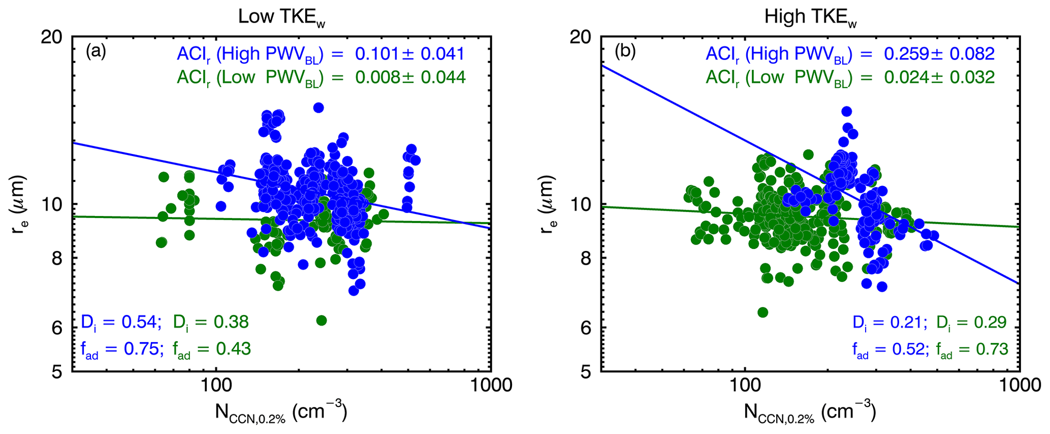
Figure 7 ACI_r derived from r_e in relation to N_CCN,0.2 % for (a) low-TKE_w and (b) high-TKE_w regimes. Samples in the low-PWV regime are plotted in green, and samples in the high-PWV regime are plotted in blue. The mean values of D_i and f_ad are displayed for each quadrant with the corresponding color coding.

The TKE_w has been found to be strongly positively correlated with W_dir,NS and negatively correlated with D_i from the PCA; that is, the values of TKE_w already account for the co-variabilities in these variables. Therefore, treating TKE_w as the sorting variable would lead to a more physical process-oriented assessment. Accordingly, to examine the role of the dynamical factors in ACI, the samples are separated into four regimes demarcated by the median values of PWV_BL and TKE_w (Fig. 7), and the mean values of D_i and f_ad in the four quadrants are also displayed in Fig. 7. The effect of PWV_BL on ACI_r is demonstrated by the mean ACI_r values where they are much higher in the high-PWV_BL regime than those in the low-PWV_BL regime no matter what the TKE_w regimes are. Furthermore, the result illustrates that TKE_w does play an important role in ACI_r because the ACI_r values in the high-TKE_w regime are more than double the values in the low-TKE_w regime.

In the regimes of high TKE_w and PWV_BL, which are closely associated with coupled MBL (D_i=0.21) and more sub-adiabatic cloud conditions (f_ad=0.52), r_e is highly sensitive to CCN loading with a highest ACI_r of 0.259. The sufficient water vapor availability allows CCN to be converted into cloud droplets more effectively, while the higher TKE_w indicates stronger turbulence in the below-cloud boundary layer and maintains a nearly well mixed MBL. The CCN and moisture below-cloud layer are efficiently transported and mixed aloft via the ascending branch of the eddies (Nicholls, 1984; Hogan et al., 2009); hence they are effectively connected to the cloud layer. Therefore, under the lower CCN loading condition, the active coalescence process (which indicated by the low f_ad values) results in the depletion of small cloud droplets and broadening of cloud DSD (Chandrakar et al., 2016) and, in turn, leads to further enlarged r_e. However, with higher CCN intrusion into the cloud layer, the enhanced cloud droplet conversion and the subsequential condensational growth behave contradictorily to narrow the DSD (Pinsky and Khain, 2002; Pawlowska et al., 2006), which leads to decreased r_e. Therefore, the MBL clouds are distinctly susceptible to CCN loading under the environments of sufficient water vapor and strong turbulence in which the ACI_r is enlarged.

Under high PWV_BL but low TKE_w conditions, the mean ACI_r is reduced to 0.101 (∼ 39 % of that under high TKE_w). The MBL is more likely decoupled where D_i=0.54, which indicates that the weaker turbulence loosens the connection between the cloud layer and the underlying boundary layer. This results in a less effective conversion of CCN into cloud droplets, while the more adiabatic cloud environment (f_ad=0.75) denotes the lack of coalescence growths and thus diminishes the r_e sensitivity to CCN. Although the constraints of insufficient water vapor on ACI_r are still evident, the ACI_r values increase from 0.008 in the low-TKE_w regime to 0.024 in the high-TKE_w regime. The ACI_r differences between the two TKE_w regimes attest that ACI_r strongly depends on the connection between the cloud layer and the below-cloud boundary layer CCN and moisture; that is, stronger turbulence can enhance the susceptibility of r_e to CCN.

In this study, the relationship between turbulence and ACI is found to be valid in non-precipitating MBL clouds. Theoretically, the effect of turbulence on ACI_r would appear to be artificially amplified if in the presence of precipitation. The intensive turbulence can enhance the coalescence process and accelerate the CCN–cloud cycling, and subsequently, the CCN depletion due to precipitation and coalescence scavenging would result in quantitatively enlarged ACI_r (Feingold et al., 1996, 1999; Duong et al., 2011; Braun et al., 2018). Though it is beyond the scope of this study, it would be of interest to perform such analysis on the aerosol–cloud–precipitation interaction using ground-based remote sensing and model simulations in a future study.

4 Summaries and conclusions

Over the ARM-ENA site, a total of 20 non-precipitating single-layered MBL stratus and stratocumulus cloud cases have been selected in order to investigate the aerosol–cloud interaction (ACI). The distributions of CCN and cloud properties for selected cases represent the typical characteristics of non-precipitating MBL clouds in a relatively clean environment over the remote oceanic area. The diversity of boundary layer conditions and cloud adiabaticities among the selected cases enables the investigation of different environmental effects on ACI.

The overall variations in N_c with N_CCN,0.2 % show an increasing trend, regardless of the water vapor condition, while the sufficient PWV_BL appears to stabilize the CCN–N_c conversion process. The water vapor limitation on cloud droplet growth is evident in the lower N_CCN,0.2 % of up to 150 cm⁻³ with low PWV_BL values, where a near tripling of CCN loading leads to a near doubling of N_c but only a 4.7 % increase in r_e. When N_CCN,0.2 % is greater than 250 cm⁻³ and PWV_BL values are also relatively high, r_e appears to decrease with increasing N_CCN,0.2 % under similar water vapor conditions. As for bulk aerosol–cloud interaction, the ACI_r values vary from −0.01 to 0.22 for different PWV_BL conditions where ACI_r appears to be diminished under limited water vapor availability due to limited droplet activation and condensational growth processes. While under relatively sufficient water supply conditions, r_e shows more sensitive responses to the changes in N_CCN,0.2 % due to the combined effect of condensational growth and coalescence processes accompanying the higher N_c and PWV_BL.

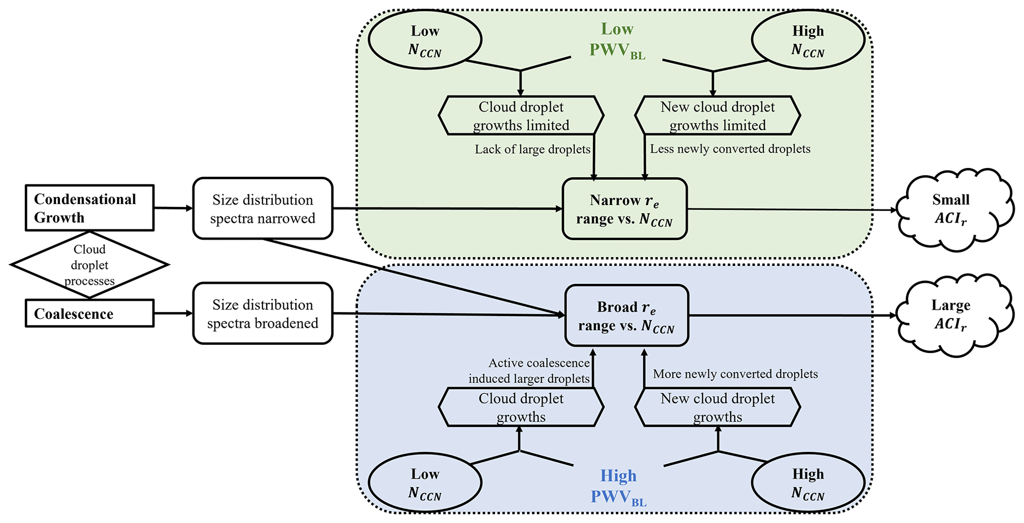
Figure 8 Theoretical mechanism of the responses of cloud droplet size distributions to different CCN intrusions, under relatively insufficient (low PWV_BL) versus sufficient (high PWV_BL) water vapor availabilities.

The theoretical diagram describing the mechanism proposed above is shown in Fig. 8. Under the lower PWV_BL condition, the limited water vapor weakens the ability of condensational growth of the cloud droplet converted from CCN, which results in both fewer newly converted and fewer large cloud droplets, with a lack of chance of coalescence processes under this circumstance. Therefore, the variable range of r_e versus N_CCN,0.2 % is narrowed and presented as small ACI_r values, while under the higher PWV_BL condition, particularly in low CCN conditions, the sufficient water vapor availability allows cloud droplets to grow via the condensation of water vapor, and thus the active cloud droplet coalescence regime is entered. In contrast, the increase in cloud droplet size can effectively reduce N_c via the coalescence process and the size distributions are effectively broadened toward a large tail by the coalescence, so r_e is enlarged. Under a higher N_CCN,0.2 % intrusion, the cloud droplet size distribution is narrowed by the enhanced condensational growth and regresses toward a small tail by increasing the number of newly converted cloud droplets, which results in decreased r_e. Combined, the interactions between CCN and cloud droplet growth processes ultimately result in a broadened changeable range of r_e and, in turn, enlarged ACI_r.

The co-variabilities among the environmental factors are examined using the multi-dimensional PCA. The variables of PWV_BL, D_i, TKE_w, LTS, and W_dir,NS are constructed as the input of the eigenanalysis. Results show that the first three PCs can describe the majority (∼ 84 %) of the variance among the selected variables. The most explanatory PC1 (accounting for a 43.72 % contribution) is strongly correlated with PWV_BL and D_i (both negatively) and TKE_w (positively) and hence describes the co-variation in the boundary layer conditions, while PC2 and PC3 (accounting for 22.01 % and 18.26 % contributions, respectively) are strongly correlated with LTS and W_dir,NS, which likely indicates the variations in the Azores High position and strength. By projecting the variables onto PC1 and PC2, the PCA loading analysis shows that TKE_w is strongly negatively correlated with D_i, which is what we expected. A decoupled MBL cloud is often separated into two layers where the lower one can cap the surface moisture, while the higher TKE_w denotes sufficient turbulence that maintains the well-mixed MBL. Additionally, the island effect is also indicated by the eigenanalysis, where surface northerly wind would induce additional updraft velocity and hence disturb TKE_w, owing to the effect of the cliff north of the ENA site. The role of cloud adiabaticities on the behaviors of CCN–N_c conversion is examined using both binning and eigenanalysis. In a near-adiabatic cloud vertical structure, the cloud droplet growth process is dominated by condensational growth; thus the N_c responses to increased N_CCN,0.2 % and PWV_BL are strengthened. When the cloud layer becomes more sub-adiabatic, the effect of coalescence leads to the depletion of N_c and thus results in the lower retrieved N_c from a ground-based snapshot perspective. The competition between the condensational growth and coalescence processes strongly impacts the variations in cloud microphysics in relation to CCN loading.

To investigate the environmental effects on ACI_r, the factors having the most influence on the explanatory PCs are selected as the sorting variables in the ACI_r assessments. The LTS sorting method cannot distinguish between the ACI_r values, which means the LTS values themselves have a weak impact on ACI_r due to the MBL cloud cover over the ENA being mainly impacted by the mid-latitude cyclone systems. In contrast, the intensity of boundary layer turbulence represented by TKE_w plays a more important role in ACI_r, since the values of TKE_w already account for the co-variations in the MBL conditions, and hence leads to a physical process-oriented assessment. The ACI_r assessments in four different TKE_w and PWV_BL regimes show that the constraints of insufficient water vapor on the ACI_r are still evident, but in both PWV_BL regimes, the ACI_r values more than double from low-TKE_w to high-TKE_w regimes. Noticeably, the ACI_r increases from 0.101 in the low-TKE_w regime to 0.259 in the high-TKE_w regime, under high PWV_BL conditions. The intensive below-cloud boundary layer turbulence strengthens the connection between the cloud layer and below-cloud CCN and moisture. So with sufficient water vapor, active coalescence leads to further enlarged r_e, particularly for low CCN loading conditions, while the enhanced N_c from condensational growth induced by increased N_CCN,0.2 % can effectively decrease r_e. Combining these processes together, the enlarged ACI_r is presented.

In this study, the non-precipitating MBL clouds are found to be most susceptible to the below-cloud CCN loading under environments with sufficient water vapor and stronger turbulence. This study examines the importance of the environmental effects on the ACI_r assessments and provides observational constraints to future model evaluations of aerosol–cloud interactions. Future studies will be focusing on exploring the role of environmental effects on the aerosol–cloud–precipitation interactions in MBL stratocumulus through an integrative analysis of observations and model simulations.